Quantum versus Population Dynamics over Cayley GraphsThanks: This work was supported by the U.S. National Science Foundation through the grants DMR-1823800 and CMMI-2131760.

Cayley graphs encode the data of a group in a geometric fashion [9]. For example, word problems and other theoretical problems in group theory can be solved by inspecting these geometric objects. On the applied side, Cayley graphs can be used to generate systematic generalizations of the crystal lattices investigated in materials science. Hence they can be an abundant source of new dynamical effects, which is our main motivation for studying them.

In this definition, $S$ can any finite subset of $G$ and one should be aware that the geometry of the Cayley graph depends quite strongly on the choice of $S$. As we shall see in the explicit examples, the choice of this set $S$ is dictated by the particular models that are investigated. Many groups, however, have standard presentations in terms of generators and relations and, in such cases, there are the particular Calyley graphs that are constructed from the finite set of generators. We call them the standard Cayley graphs of the groups and denote them simply by ${\mathcal{C}}(G)$. Below, we supply two examples showcasing the beauty of the Cayley graphs:

A more refined geometric object is the Cayley diagraph:

Let ${\mathcal{C}}(G)$ be the standard Cayley graph of a discrete group $G$. We populate the nodes of this graph with identical objects, which we will call chips from now on, and denote by $N_{g}$ the number of chips stacked at node $g$. We are seeking algorithms that take $\{N_{g}\}_{g\in G}$ as input and return new values $\{N^{\prime}_{g}\}_{g\in G}$, in a manner that respects the symmetry of the graph, in the sense that, if $\{N_{g}\}_{g\in G}\mapsto\{N^{\prime}_{g}\}_{g\in G}$, then $\{N_{gg^{\prime}}\}_{g\in G}\mapsto\{N^{\prime}_{gg^{\prime}}\}_{g\in G}$ if the algorithm is applied to $\{N_{gg^{\prime}}\}_{g\in G}$. In other words, the algorithm is invariant to the translations of the Cayley graph. Additionally, we require that the number of chips be preserved. Then, a repeated application of the algorithm will generate a discrete dynamics for the population of chips.

For this, let $S=\{g_{1},\ldots,g_{s}\}$ be a finite sub-set of the group $G$ and consider the following protocol. The stack of $N_{g}$ chips sitting at site $g$ is divided in $s$ smaller stacks containing $N_{g}^{j}:=p_{j}N_{g}$ chips, $j=1,\ldots,s$, where $p_{j}\in[0,1]$ are fixed predefined weights that add to one: $p_{1}+\cdots+p_{s}=1$. After this operation is completed for each $g\in G$, the stack of $N_{g}^{j}$ chips is moved at the site $g_{j}g$, and this step is repeated for $g$’s and $j$’s. For finite groups, the processes we just described can be carried manually or it can be automated. Let us point out that sometimes the dynamics generated in this way can be understood more effectively if we pass from from the standard Cayley graph of $G$ to the Cayely graph generated by the set $S$. This will certainly be the case for all our applications.

At a more formal level, if the population is encoded in the vector

$$|\psi\rangle=\sum_{g}N_{g}|g\rangle\in\ell^{2}(G),$$

(2.1)

then the dynamics we just described is given by $|\psi\rangle\mapsto D|\psi\rangle$, where

$$D=\sum_{j=1}^{s}\sum_{g\in G}p_{j}\,|g_{j}g\rangle\langle g|.$$

(2.2)

Thus the operator $D$ generates the dynamics and, as such, it will be called the dynamical matrix. We point out that $D$ is a self-adjoint operator if and only if the set $S$ is invariant under taking the inverse of its elements and if $p_{j}=p_{i}$ whenever $g_{i}$ is the inverse of $g_{j}$.

Using this formal description of the dynamics, it is easy to see that the proposed algorithms respect the two constraints we stated above. Indeed, the right action of the group $G$ on itself induces the right regular representation $\pi_{R}$ of $G$ on $\ell^{2}(G)$:

$$U_{g}|g^{\prime}\rangle=|g^{\prime}g^{-1}\rangle,\hskip 8.19447ptg,g^{\prime}\in G.$$

(2.3)

These operations are often called the translations of Cayley graph. Then one can easily check that the dynamics is invariant relative to this group action:

$$\pi_{R}(g)D=D\pi_{R}(g),\hskip 8.19447pt\forall\ g\in G.$$

(2.4)

Indeed, on the basis $|g^{\prime}\rangle$ of $\ell^{2}(G)$, we have

$$\pi_{R}(g)D|g^{\prime}\rangle=\sum_{j=1}^{s}p_{j}|(g_{j}g^{\prime})g^{-1}\rangle=\sum_{j=1}^{s}p_{j}|g_{j}(g^{\prime}g^{-1})\rangle=D\pi_{R}(g)|g^{\prime}\rangle.$$

(2.5)

Thus, our protocols respect the symmetry of the Cayley graphs, a feature that is automatically present due to the associativity of the group multiplication rule.

Furthermore, due to our constraint on the weights $\{p_{j}\}$, the uniform state $\psi_{0}$ is a right and a left eigenvector of the dynamical matrix, which is not assumed self-adjoint:

$$|\psi_{0}\rangle:=\sum_{g\in G}|g\rangle,\hskip 8.19447ptD|\psi_{0}\rangle=|\psi_{0}\rangle,\hskip 8.19447ptD^{\dagger}|\psi_{0}\rangle=|\psi_{0}\rangle.$$

(2.6)

In fact, it is important to note that if $\psi_{0}$ is a left eigenvector of $D$ then it is automatically also a right eigenvector (i.e. a left eigenvector for $D^{\dagger}$). Now, note that if $|\psi\rangle$ is any state of the population of chips, then

$$\langle\psi_{0}|\psi\rangle=\sum_{g\in G}N_{g},$$

(2.7)

which supplies a convenient way to compute the total number of chips carried by the state $\psi$. Now, computing the number of chips for the time evolved state $D|\psi\rangle$, we get

$$\langle\psi_{0}|D|\psi\rangle=\langle D^{\dagger}\psi_{0}|\psi\rangle=\langle\psi_{0}|\psi\rangle,$$

(2.8)

hence the number of chips is conserved by the dynamics. An important conclusion is that $\psi_{0}$ being an eigenvector of $D$ with eigenvalue 1 is a simple necessary and sufficient condition for the conservation of chips during the dynamics.

Given a discrete group $G$, its group algebra ${\mathbb{C}}G$ consists of formal series

$$q=\sum_{g\in G}\alpha_{g}\,g,\hskip 8.19447pt\alpha_{g}\in{\mathbb{C}},$$

(2.9)

where all but a finite number of terms are zero. Addition and multiplication of such formal series work in the obvious way using the group and algebraic structures of $G$ and ${\mathbb{C}}$, respectively. In addition, there exists a natural $\ast$-operation

$$q^{\ast}=\sum_{g\in G}\bar{\alpha}_{g}\,g^{-1},\hskip 8.19447pt(q^{\ast})^{\ast}=q,\hskip 8.19447pt(\alpha q)^{\ast}=\bar{\alpha}q^{\ast},\ \alpha\in{\mathbb{C}},$$

(2.10)

where the bar indicates complex conjugation. Hence, ${\mathbb{C}}G$ is naturally a $\ast$-algebra.

We denote by $e$ the neutral element of $G$. Then the map

$${\mathcal{T}}:{\mathbb{C}}G\to{\mathbb{C}},\hskip 8.19447pt{\mathcal{T}}(q)=\alpha_{e},$$

(2.11)

defines a positive trace on ${\mathbb{C}}G$ and a pre-Hilbert structure on ${\mathbb{C}}G$ via

$$\langle q,q^{\prime}\rangle:={\mathcal{T}}(q^{\ast}q^{\prime}),\hskip 8.19447ptq,q^{\prime}\in{\mathbb{C}}G.$$

(2.12)

The completion of the linear space ${\mathbb{C}}G$ under this pre-Hilber structure supplies the Hilbert space $\ell^{2}(G)$. Indeed, one can verify that

$$\langle g,g^{\prime}\rangle=\delta_{g,g^{\prime}},\hskip 8.19447ptg,g^{\prime}\in G.$$

(2.13)

The action of ${\mathbb{C}}G$ on itself can be extended to the action of a bounded operator on $\ell^{2}(G)$, and this supplies the left regular representation inside ${\mathbb{B}}\big(\ell^{2}(G)\big)$, denoted by $\pi_{L}$ in the following. Specifically,

$$\pi_{L}(q)|g^{\prime}\rangle=\sum_{g}\alpha_{g}|gg^{\prime}\rangle,\hskip 8.19447ptq\in{\mathbb{C}}G,\hskip 8.19447ptg^{\prime}\in G.$$

(2.14)

Now, if $p=\sum_{j=1}^{s}p_{j}\,g_{j}$, then $\pi_{L}(p)$ is exactly the generator (2.2) of the dynamics defined by our protocols. Also, note that $\pi_{L}(p^{\ast})=\pi_{L}(p)^{\dagger}$ and that

$$\big(\sum_{j=1}^{s}p_{j}\,g_{j}\big)^{\ast}=\sum_{j=1}^{s}p_{j}\,g_{j}^{-1},$$

(2.15)

from where we can quickly see when a dynamical matrix is self-adjoint or not. The main point here is that any dynamical matrix can be canonically generated from ${\mathbb{C}}G$ and the dynamics can be studied entirely inside ${\mathbb{C}}G$.

We will work with the finite abelian group ${\mathbb{Z}}_{N}={\mathbb{Z}}/(N\,{\mathbb{Z}})$ and its Cayley graph. If $S$ is the generator of ${\mathbb{Z}}_{N}$, then the self-adjoint operator

$$H=\tfrac{1}{2}(S+S^{\ast})=\tfrac{1}{2}\sum_{n\in{\mathbb{Z}}_{N}}(|n+1\rangle\langle n|+|n\rangle\langle n+1|)$$

(3.1)

can generate a quantum dynamics for, say, an electron hopping on a molecular chain, or a population dynamics via the algorithms described in the previous section. At the level of states, however, even for this simple case, there are major differences between the quantum and population dynamics. Indeed, the quantum states can have complex coefficients, while the states encoding a population must have real positive coefficients. Note that the eigenvalue problem $H\psi=\epsilon\psi$ is solved by the pairs

$$\Big\{\psi_{k}={\mathcal{N}}\sum_{n\in{\mathbb{Z}}_{N}}e^{\frac{\imath 2\pi kn}{N}}|n\rangle,\ \epsilon_{k}=\cos\big(\tfrac{2\pi k}{N}\big)\Big\}_{k\in{\mathbb{Z}}_{N}},$$

(3.2)

and, as we can see, all eigenvectors involve complex or negative coefficients, except for the uniform state $\psi_{0}$. The sad conclusion is that these eigenstates and their characteristics cannot be observed or demonstrated with the standard population evolution. Furthermore, for example, the following self-adjoint operator

$$H=\tfrac{1}{4}(S+S^{\ast}+\imath S-\imath S).$$

(3.3)

can generate a quantum dynamics, but by no means it can generate a population dynamics. Indeed, the coefficients entering the dynamical matrices must all be real and positive. Lastly, if $H$ is quantum Hamiltonian with real or complex coefficients, at first sight, there seems to impossible to simulate its quantum dynamics $e^{\imath tH}|\psi\rangle$ with population dynamics.

Mathematically, the difference between the quantum and population dynamics over a Cayledy graph ${\mathcal{C}}(G)$, is that the former is associated to the group algebra ${\mathbb{C}}G$ and its left regular representation, while the latter is associated with the semi-ring ${\mathbb{R}}_{+}G$ and its left-regular representation. Indeed, in the latter case, both the states and the Hamiltonians are constraint to take positive real values.

However, let us point out a close relation between the field of complex numbers ${\mathbb{C}}$ and the semi-ring ${\mathbb{R}}_{+}{\mathbb{Z}}_{4}$, which is the backbone of our solution. For this, let $\xi$ be the generator of ${\mathbb{Z}}_{4}$, hence ${\mathbb{Z}}_{4}=\{1,\xi,\xi^{2},\xi^{3}\}$ and an element of ${\mathbb{R}}_{+}{\mathbb{Z}}_{4}$ accepts a unique presentation as

$$\sum_{j=0}^{3}\beta_{j}\xi^{j},\hskip 8.19447pt\beta_{j}\in{\mathbb{R}}_{+}.$$

(3.4)

On the other hand, the field ${\mathbb{C}}$ of complex numbers is also a ring, hence also a semi-ring. Then, viewing ${\mathbb{C}}$ as a semi-ring, we note the surjective semi-ring morphism $\chi:{\mathbb{R}}_{+}{\mathbb{Z}}_{4}\to{\mathbb{C}}$ defined by

$$\chi(1)=1,\ \ \chi(\xi)=\imath,\ \ \chi(\xi^{2})=-1,\ \ \chi(\xi^{3})=-\imath.$$

(3.5)

It has a non-trivial kernel given by the ideal

$${\rm ker}\,\chi=(1+\xi^{2})\cdot{\mathbb{R}}_{+}{\mathbb{Z}}_{4}.$$

(3.6)

All this information can be summarized as the following exact sequence:

$$0\to(1+\xi^{2})\cdot{\mathbb{R}}_{+}{\mathbb{Z}}_{4}\to{\mathbb{R}}_{+}{\mathbb{Z}}_{4}\to{\mathbb{C}}\simeq{\mathbb{R}}_{+}{\mathbb{Z}}_{4}/(1+\xi^{2})\cdot{\mathbb{R}}_{+}{\mathbb{Z}}_{4}\to 0.$$

(3.7)

The conclusion is that the field ${\mathbb{C}}$ can be generated as the quotient semi-ring

$${\mathbb{C}}={\mathbb{R}}_{+}{\mathbb{Z}}_{4}/(1+\xi^{2})\cdot{\mathbb{R}}_{+}{\mathbb{Z}}_{4}$$

(3.8)

and the quotient map, of course, coincides with the map $\chi$ defined above. Furthermore, the exact sequence (3.7) is not split at the level of semi-rings, but a particularly relevant section (i.e. a right inverse for $\chi$, $\chi\circ\mathfrak{s}={\rm id}$) exists at the level of linear spaces:

$${\mathbb{C}}\ni z=a+\imath b\mapsto\mathfrak{s}(z)=|a|\,\xi^{1-{\rm sgn}(a)}+|b|\,\xi^{2-{\rm sgn}(b)}\in{\mathbb{R}}_{+}{\mathbb{Z}}_{4}.$$

(3.9)

In fact, both ${\mathbb{C}}$ and ${\mathbb{R}}_{+}{\mathbb{Z}}_{4}$ have a structure of ${\mathbb{R}}_{+}$-modules and $\mathfrak{s}$ is a homomorphism of such semi-modules:

$$\mathfrak{s}(rz)=r\mathfrak{s}(z),\hskip 8.19447pt\forall\ r\in{\mathbb{R}}_{+}.$$

(3.10)

Now, in order to use this simple observation to the problem of quantum and population dynamics over ${\mathcal{C}}(G)$, we pass to the ordinary group product ${\mathbb{Z}}_{4}\times G$ and consider population dynamics over its Cayley graphs. In this case, the generators of the dynamics come from the group semi-ring

$${\mathbb{R}}_{+}({\mathbb{Z}}_{4}\times G)\simeq({\mathbb{R}}_{+}{\mathbb{Z}}_{4})G.$$

(3.11)

An element of this semi-ring is a formal finite sum

$$\tilde{q}=\sum_{g\in G}\tilde{\alpha}_{g}\,g,\hskip 8.19447pt\tilde{\alpha}_{g}\in{\mathbb{R}}_{+}{\mathbb{Z}}_{4}.$$

(3.12)

Note that the commutative semi-ring ${\mathbb{R}}_{+}{\mathbb{Z}}_{4}$ is canonically embedded in $({\mathbb{R}}_{+}{\mathbb{Z}}_{4})G$ via

$${\mathbb{R}}_{+}{\mathbb{Z}}_{4}\ni\tilde{\alpha}\mapsto\tilde{\alpha}\,e\in({\mathbb{R}}_{+}{\mathbb{Z}}_{4})G.$$

(3.13)

Obviously $(\tilde{\alpha}\,e)\tilde{q}=\tilde{q}(\tilde{\alpha}\,e)$, hence $({\mathbb{R}}_{+}{\mathbb{Z}}_{4})G$ has a structure of semi-algebra over the commutative ring ${\mathbb{R}}_{+}{\mathbb{Z}}_{4}$.

The essential observation is that $(1+\xi^{2})\cdot({\mathbb{R}}_{+}{\mathbb{Z}}_{4})G$ is an ideal of the above semi-ring and that

$$({\mathbb{R}}_{+}{\mathbb{Z}}_{4})G/(1+\xi^{2})\cdot({\mathbb{R}}_{+}{\mathbb{Z}}_{4})G\simeq{\mathbb{C}}G.$$

(3.14)

The quotient map from $({\mathbb{R}}_{+}{\mathbb{Z}}_{4})G$ to ${\mathbb{C}}G$ is implemented by a straightforward extension of the map $\chi$ (denote by the same symbol $\chi$):

$$({\mathbb{R}}_{+}{\mathbb{Z}}_{4})G\ni\sum_{g\in G}\tilde{\alpha}_{g}\,g\mapsto\sum_{g\in G}\chi(\tilde{\alpha}_{g})\,g\in{\mathbb{C}}G.$$

(3.15)

It is important to keep in mind that this map, denoted by the same symbol $\chi$, is a semi-ring homomorphism. Thus, it respects the addition and multiplication operations and, as such, it commutes with the functional calculus, in the sense that

$$\chi\big(\phi(\tilde{q})\big)=\phi\big(\chi(\tilde{q}))$$

(3.16)

for any polynomial $\phi$. Lastly, the section defined in Eq. (3.9) extends to a right inverse for $\eta$,

$${\mathbb{C}}G\ni\sum_{g\in G}\alpha_{g}\,g\mapsto\sum_{g\in G}\mathfrak{s}(\alpha_{g})\,g\in({\mathbb{R}}_{+}{\mathbb{Z}}_{4})G.$$

(3.17)

This extension will be denoted by the same symbol $\mathfrak{s}$ and note that $\mathfrak{s}$ is a homomorphism between ${\mathbb{R}}_{+}$-modules.

The map $\chi$ and its right inverse $\mathfrak{s}$ are our essential tools that will enable us to port models from ${\mathbb{C}}G$ into models from ${\mathbb{R}}_{+}({\mathbb{Z}}_{4}\times G)$ and, as such, to simulate a quantum dynamics on ${\mathcal{C}}(G)$ with a population dynamics over ${\mathcal{C}}({\mathbb{Z}}_{4}\times G)$. Specific experiments enabled by our solution will are discussed next.

One interesting experiment is visualization of stationary quantum states. Specifically, if $H$ is a quantum Hamiltonian and $\psi_{\epsilon}$ is an eigenvector $H\psi_{\epsilon}=\epsilon\psi_{\epsilon}$, we can generate a dynamical matrix and an initial state for a population dynamics on ${\mathcal{C}}({\mathbb{Z}}_{4}\times G)$ as

$$\tilde{D}=\mathfrak{s}(H),\hskip 8.19447pt|\tilde{\psi}_{\epsilon}\rangle=|\mathfrak{s}(\psi_{\epsilon})\rangle,$$

(3.18)

where for $\tilde{\psi}$ we used Remark 2.8. We can then use our algorithm to time-evolve the population

$$|\tilde{\psi}_{\epsilon}(t)\rangle:=\tilde{D}^{t}|\tilde{\psi}_{\epsilon}\rangle,\hskip 8.19447ptt\in{\mathbb{N}}.$$

(3.19)

Projecting back on ${\mathbb{C}}G$ and its left regular representation, we will find that

$$\big|\chi\big(\tilde{\psi}_{\epsilon}(t)\big)\big\rangle=\chi\Big(\tilde{D}^{t}|\tilde{\psi}_{\epsilon}\rangle\Big)=\chi\big(\tilde{D}^{t}\big)|\chi(\tilde{\psi}_{\epsilon})\rangle=\chi\big(\tilde{D}\big)^{t}|\psi_{\epsilon}\rangle=H^{t}|\psi_{\epsilon}\rangle,$$

(3.20)

hence, apart from a scaling factor, this projected state is stationary under the discrete time evolution. As one can see, the property of the map $\chi$ of respecting the addition and multiplication is essential for our arguments.

To be effective, we must supply an experimental protocol for applying the quotient map (3.15). For this, an experimenter examines a coefficient $\tilde{\alpha}_{g}=\sum_{j=0}^{3}\alpha_{g}^{j}\xi^{j}$, which is encoded in the four stacks $\alpha_{g}^{j}$ of chips. Now,

$$\chi(\tilde{\alpha}_{g})=\alpha_{g}^{0}-\alpha_{g}^{3}+\imath(\alpha_{g}^{1}-\alpha_{g}^{4}),$$

(3.21)

thus, the experimenter simply needs to compare the stacks $\alpha_{g}^{0}$ and $\alpha_{g}^{3}$ of chips, remove a number of chips from a stack such that the two stacks remain with equal number of chips, and place those chips in a stack called $\alpha_{g}^{r}$ above the zero level if $\alpha_{g}^{0}>\alpha_{g}^{3}$ and below the zero level otherwise. Similarly from the stacks $\alpha_{g}^{1}$ and $\alpha_{g}^{4}$, the experimenter creates the stack $\alpha_{g}^{i}$. For a state

$$|\tilde{\psi}\rangle=\sum_{g\in G}\tilde{\alpha}_{g}|g\rangle=\sum_{j=0}^{3}\sum_{g\in G}\alpha_{g}^{j}|\xi^{j},g\rangle\in\ell^{2}({\mathbb{Z}}_{4}\times G),$$

(3.22)

by repeating the procedure for all $\tilde{\alpha}_{g}$’s, the experimenter creates the stacks $\{\alpha_{g}^{r},\alpha_{g}^{i}\}$ encoding the real and imaginary parts of $|\chi(\tilde{\psi})\rangle$. This gives a simple protocol for visualizing quantum states with a population of chips.

Another class of quantum experiments that can be simulated with a population of chips is visualizing the time evolution of a quantum state

$$|\psi(t)\rangle=e^{\imath tH}|\psi\rangle,\hskip 8.19447ptt\in{\mathbb{R}}_{+}.$$

(3.23)

For this, we use the standard approximation of the exponential function

$$e^{\imath tH}=\lim_{m\to\infty}\big(1+\tfrac{\imath t}{m}H\big)^{m}$$

(3.24)

and generate a dynamical matrix and an initial population of chips

$$\tilde{D}=\gamma\,\mathfrak{s}\big(1+\tfrac{\imath t}{m}H\big),\hskip 8.19447pt|\tilde{\psi}(0)\rangle=|\mathfrak{s}(\psi)\rangle,$$

(3.25)

where $\gamma$ is a positive factor that ensures that the number of chips are conserved. We then perform the discrete time evolution

$$|\tilde{\psi}(k)\rangle=\tilde{D}|\tilde{\psi}(k-1)\rangle,\hskip 8.19447ptk=1,\ldots,m,$$

(3.26)

on the Cayley graph of ${\mathbb{Z}}_{4}\times G$ and finally project back on ${\mathbb{C}}G$ and its left regular representation, to find:

$$\gamma^{-m}\,\big|\chi\big(\tilde{\psi}(m)\big)\big\rangle=\gamma^{-m}\,\chi\big(\tilde{D}\big)^{m}|\chi(\psi)\rangle=\big(1+\tfrac{\imath t}{m}H\big)^{m}|\psi\rangle\approx e^{\imath tH}|\psi\rangle.$$

(3.27)

Concrete experiments along these lines are presented in the next section.

In this experiment, we will demonstrate and visualize a stationary quantum state. For this, we consider the quantum Hamiltonian $H=\frac{1}{2}(S+S^{\ast})$ introduced in Sec. 3, which now is viewed as an element of ${\mathbb{R}}_{+}({\mathbb{Z}}_{4}\times{\mathbb{Z}}_{N})$. To convey this fact, we will work with $\tilde{D}=\mathfrak{(}H)$, even though $\tilde{D}$ has the same expression as $H$. Fig. 4.1 shows the Cayley diagraph corresponding to the group ${\mathbb{Z}}_{4}\times{\mathbb{Z}}_{N}$ and element $S\in{\mathbb{Z}}_{N}$. We call this the ${\mathbb{Z}}_{4}$-decorated Cayley graph. For the Hamiltonian (3.1), the decorated dynamics remains very simple because this Hamiltonian has real positive coefficients.

Now, we choose a state $\psi_{k}$ as in Eq. (3.2) and ported it on $\ell^{2}({\mathbb{Z}}_{4}\times{\mathbb{Z}}_{N})$ using the section $\mathfrak{s}$ from Eq. (3.17):

	$\displaystyle\tilde{\psi}_{k}=\mathfrak{s}(\psi_{k})={\mathcal{N}}\sum_{n\in{\mathbb{Z}}_{N}}$	$\displaystyle\big[|\cos\big(\tfrac{2\pi kn}{N}\big)|\big|\xi^{1-{\rm sgn}(\cos(\frac{2\pi kn}{N}))},n\big\rangle$		(4.1)
		$\displaystyle+|\sin\big(\tfrac{2\pi kn}{N}\big)|\big|\xi^{1-{\rm sgn}(\sin(\frac{2\pi kn}{N}))},n\big\rangle\big].$

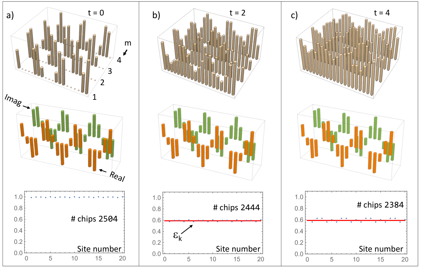
The population corresponding to this state is reported in the top row of Fig. 4.2(a), together with the visualization of $\chi(\tilde{\psi}_{k})$ (second row) and a comparison between $\chi(\tilde{\psi}_{k})$ and $\psi_{k}$ (third row), for $k=1$. The data seen in this figure confirms that the maps $\chi$ and $\mathfrak{s}$ work as expected. Same information is reported in Fig. 4.3(a) for the stationary state generated with $k=3$. Panels (b) and (c) in Fig. 4.2(a) report the states $|\tilde{\psi}(t)\rangle=\tilde{D}^{t}|\tilde{\psi}\rangle$ for $t=5$ and $t=10$, respectively, visualizations of $|\psi(t)\rangle=\big|\chi\big(\tilde{\psi}(t)\big)\big\rangle$, together with checks of their expected relations $|\psi(t)\rangle=\epsilon_{k}|\psi(t-1)\rangle$. Same information is reported in Fig. 4.3(b,c) for the case $k=3$ and times $t=2$ and $t=4$, respectively.

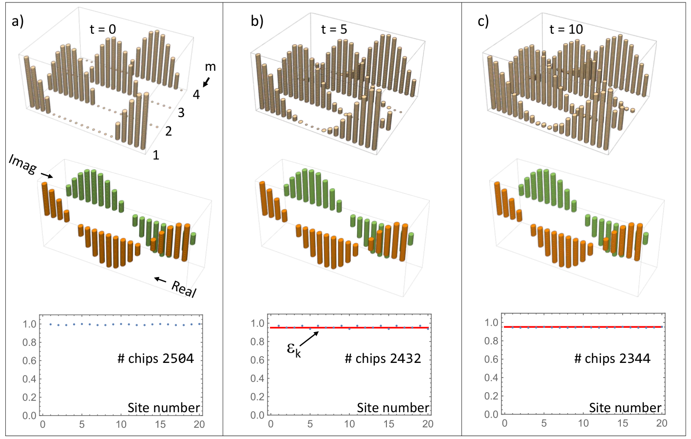
These experiments reveal several interesting observations. First, the time-evolved population dynamics on the ${\mathbb{Z}}_{4}$-decorated graph produces somewhat complicated states, yet the projection onto the original graph, using the protocol described in the previous section, produces clear stationary states. As we already explained, there is a loss of chips during the dynamics, but this obviously does not affect the demonstrations we actually want to show.

Here we consider the following Hamiltonian on $\ell^{2}({\mathbb{Z}}_{N})$:

$$H=\tfrac{1}{4}(S+S^{\ast}+\imath S-\imath S).$$

(4.2)

It has the same eigenvectors $\psi_{k}$ but with corresponding eigenvalues

$$\epsilon_{k}=\tfrac{1}{2}\big[\cos\big(\tfrac{2\pi k}{N}\big)+\sin\big(\tfrac{2\pi k}{N}\big)\big].$$

(4.3)

Note that these eigenvalues can be positive and negative as well. Having complex coefficients, the dynamics of this Hamiltonian cannot be directly associated with a population dynamics. We show, however, that its dynamics can be studied and observed with population dynamics experiments, if we use our strategy and port $H$ on $\ell^{2}({\mathbb{Z}}_{4}\times{\mathbb{Z}}_{N})$ as:

$$H\mapsto\tilde{D}=\tfrac{1}{4}(S+S^{\ast}+\xi S+\xi^{3}S).$$

(4.4)

The dynamics of generated by $\tilde{D}$ can be understood from the Cayley diagraph corresponding to the elements involved in $\tilde{D}$, namely, $S$ and $\xi S$. This Cayley diagraph is shown in Fig. 4.1(b). Note that $\xi^{3}S^{\ast}=(\xi S)^{-1}$, so this element is already covered be the shown Cayley diagraph.

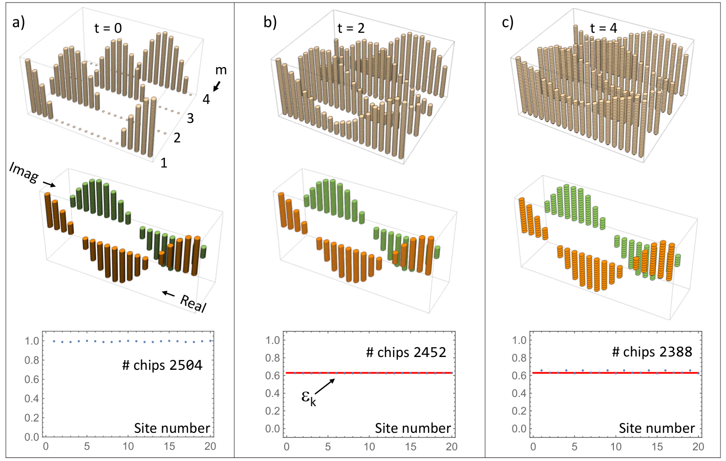
To demonstrate and visualize the stationary states of $H$, we map $\psi_{k}$ on the Cayley graph of of ${\mathbb{Z}}_{4}\times{\mathbb{Z}}_{n}$ and act with the dynamical matrix $\tilde{D}$, as it was done in the previous case. This dynamics is reported in the top row of Fig. 4.4 for the state generated with $k=1$. A projection of $\tilde{\psi}_{k}(t)$ back on the left regular representation of ${\mathbb{C}}G$ reveals again the stationary character of the quantum state $\psi_{k}$.

In this experiment, we reproduce the quantum dynamics $|\psi(t)\rangle=e^{\imath tH}|\psi(0)\rangle$, with $H$ as in Eq. (3.1) and an initial state localized entirely at one site, $\langle n|\psi(0)\rangle=\delta_{n,N/2}$. For this, we follow literally the procedure detailed in subsection 3.3 and we calculate the dynamical matrix $\tilde{D}$ introduced in Eq. (3.25), which takes the specific form

$$\tilde{D}=\gamma\big(1+\tfrac{t}{m}(\xi S+\xi S^{\ast})\big),\hskip 8.19447pt\gamma=1/(1+2t/m).$$

(4.5)

Note that this dynamical matrix is not self-adjoint but it conserves the number of chips. The initial vector on the decorated Cayley graph is simply

$$\langle j,n|\tilde{\psi}(0)\rangle=\delta_{j,1}\delta_{n,N/2},\hskip 8.19447ptj=\overline{1,4},\hskip 8.19447ptn\in{\mathbb{Z}}_{N}.$$

(4.6)

To implement the population dynamics, however, we will place a large number of chips at the location $(1,N/2)$ to ensure that the shuffling doesn’t stop due to lack of chips. This is not an isuue because, afterwards, the time-evolved states are properly normalized, hence taking out the arbitrariness introduced by this little detail.

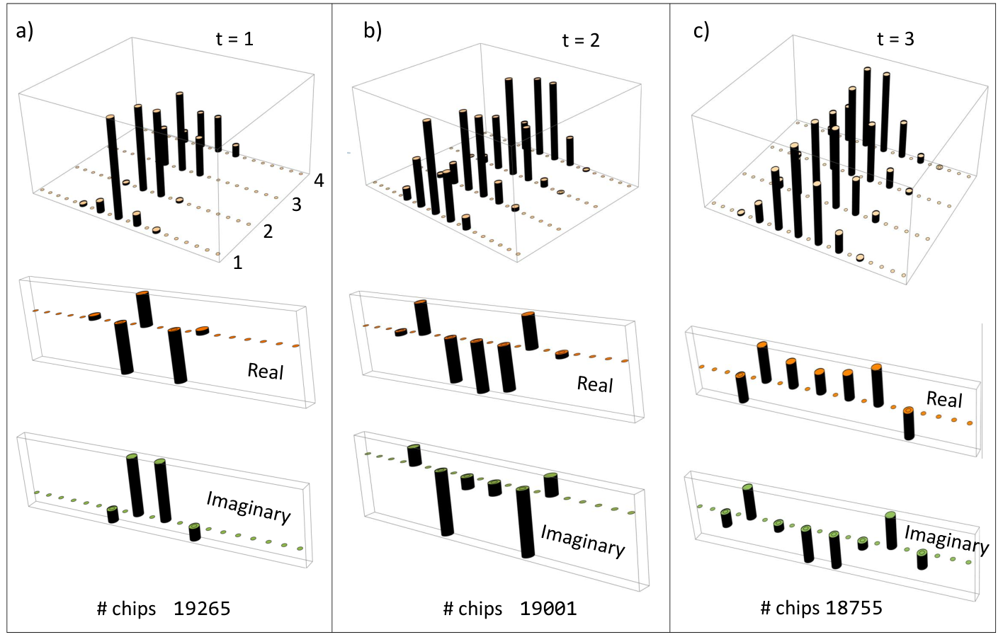
The top row of Fig. 4.5 shows the time evolution $|\tilde{\psi}(t)\rangle$ of the initial state $|\tilde{\psi}(0)\rangle$ under the dynamical matrix $\tilde{D}$ from Eq. (4.5). The second and third rows of the same figure show the real and imaginary parts of the projections $\big|\chi\big(\tilde{\psi}(t)\big)\big\rangle$ for different times. The normalizations of these population states coincide with the exact time-evolved quantum states $|\psi(t)\rangle$, up to less than 1% differences.

References

- [1] Y. Barlas, E. Prodan, Topological classification table implemented with classical passive metamaterials, Physical Review B 98, 094310 (2018).
- [2] W. Cheng, E. Prodan, C. Prodan, Experimental demonstration of dynamic topological pumping across incommensurate acoustic meta-crystals, Phys. Rev. Lett. 125, 224301 (2020).
- [3] W. Cheng, E. Prodan, C. Prodan, Revealing the boundary Weyl physics of the four-dimensional Hall effect via phason engineering in metamaterials, Phys. Rev. Applied 16, 044032 (2021).
- [4] K. Qian, D. J. Apigo, K. Padavić, K. H. Ahn, S. Vishveshwara, C. Prodan, Observation of phase controllable majorana-like bound states in metamaterial-based Kitaev chain analogues, arXiv:2201.12377 (2022).
- [5] W. Cheng, E. Prodan, C. Prodan, Topological D-class physics with passive acoustic elements, arXiv:2204.03613 (2022).
- [6] G. Engelhardt, M. Benito, G. Platero, G. Schaller, T. Brandes, Random-walk topological transition revealed via electron counting, Phys. Rev. B 96, 241404(R) (2017).
- [7] E. Tang, J. Agudo-Canalejo, R. Golestanian, Topology protects chiral edge currents in stochastic systems, Phys. Rev. X 11, 031015 (2021).
- [8] F. D. M. Haldane, Model for a quantum Hall-effect without Landau levels: Condensed-matter realization of the parity anomaly, Phys. Rev. Lett. 61, 2015–2018 (1988)
- [9] C. Löh, Geometric group theory, (Springer, Berlin, 2017).