Investigating Loop Quantum Gravity with EHT Observational Effects of Rotating Black holes
Abstract
A mathematically consistent rotating black hole model in loop quantum gravity (LQG) is yet lacking. The scarcity of rotating black hole solutions in LQG substantially hampers the development of testing LQG from observations, e.g., from the Event Horizon Telescope (EHT) observations. The EHT observation revealed event horizon-scale images of the supermassive black holes Sgr A* and M87*. The EHT results are consistent with the shadow of a Kerr black hole of general relativity. We present LQG-motivated rotating black hole (LMRBH) spacetimes, which are regular everywhere and asymptotically encompass the Kerr black hole as a particular case. The LMRBH metric describes a multi-horizon black hole in the sense that it can admit up to three horizons, such that an extremal LMRBH, unlike the Kerr black hole, refers to a black hole with angular momentum . The metric, depending on the parameters, describes (1) black holes with only one horizon (BH-I), (2) black holes with an event horizon and a Cauchy horizons (BH-II), (3) black holes with three horizons (BH-III) or (4) no-horizon (NH) spacetime, which, we show, is almost ruled out by the EHT observations. We constrain the LQG parameter with the aid of the EHT shadow observational results of M87* and Sgr A*,respectively, for an inclination angle of and . In particular, the VLTI bound for the Sgr A*, , constrains the parameters () such that for km), the allowed range of is . Together with the EHT bounds of Sgr A∗ and M87∗ observables, our analysis concludes that a substantial part of BH-I and BH-II parameter space agrees with the EHT results of M87* and Sgr A*. While the EHT M87* results totally rule out the BH-III, but not that by Sgr A*.
Keywords:
black hole physics -black hole shadow- gravitational lensing: strongI Introduction
That the gravitational collapse of a massive star () leads to a spacetime singularity in general relativity (GR) is confirmed by the elegant theorem by Hawking and Penrose (Hawking & Penrose 1970; Hawking & Ellis 1973)). However, it is widely believed that these singularities result from a classical treatment of spacetime. By its very definition, the existence of a singularity means spacetime fails to exist, signaling a breakdown in the laws of physics. Thus, singularities must be substituted by some other objects in a more unified theory for these laws to exist and will not be present when quantum effects are considered (Wheeler 1963). While we do not yet have any complete quantum gravity theory, permitting us to explore the interior of the black hole and settle it separately, we must turn our attention to regular models motivated by quantum arguments. The first regular black hole solution was proposed by Bardeen (Bardeen 1968). Bardeen asserts that although there are horizons, there is no curvature singularity. Instead, the black hole center develops a de Sitter-like region, ultimately known as a black hole with a regular center. Thus, its maximal extension is that of the Reissner–Nordström spacetime but with a regular center (Barrabes & Frolov 1996; Bronnikov et al. 2003). Thereafter, several regular black hole models have been proposed based on Bardeen’s idea, which mimics the demeanor of the Schwarzschild black hole at large distances (Poisson & Israel 1988; Dymnikova 1992; Barrabes & Frolov 1996; Bronnikov et al. 2003; Hayward 2006; Bronnikov & Fabris 2006; Simpson & Visser 2019). Also, there have been significant advances in the analysis and application of regular black holes (Ayon-Beato & Garcia 1998; Bronnikov 2001; Hayward 2006; Zaslavskii 2009; Lemos & Zanchin 2011). There is evidence that loop quantum gravity (LQG) may be competent to fix the inevitable singularities in classical GR (Ashtekar et al. 2006; Ashtekar et al. 2007; Vandersloot 2007). Because of the inherent problems in solving the complete system, the emphasis has been on spherically symmetric black holes (Ashtekar & Bojowald 2006; Modesto 2006; Boehmer & Vandersloot 2007; Campiglia et al. 2008; Gambini & Pullin 2008).
The phase space quantization or semiclassical polymerization that maintains aspects of the discreteness of underlying spacetime suggested by LQG turns out to be a fruitful technique to resolve the singularity issue, and has been used recently to significant effect (Boehmer & Vandersloot 2007; Campiglia et al. 2008; Gambini & Pullin 2008). Different polymerizations can give qualitatively other regularized spacetimes, so it is of great interest to examine a more comprehensive class of models and methods. Peltola & Kunstatter (Peltola & Kunstatter 2009a), motivated by earlier works (Ashtekar & Bojowald 2006; Modesto 2006; Boehmer & Vandersloot 2007; Boehmer & Vandersloot 2008; Campiglia et al. 2008; Gambini & Pullin 2008; Modesto 2010; Modesto 2008), used the effective field theory and the partially polymerized theory arguments to determine a static and spherically symmetric regular black hole (Peltola & Kunstatter 2009b; Peltola & Kunstatter 2009a) that is asymptotically flat. One of the most striking features of this quantum-corrected black hole, unlike other regular black holes that have two horizons, is that it has a single horizon and it also encompasses a Schwarzschild black hole.
The no-hair theorem embodies the unique qualities of the GR black hole, stating that the Kerr black hole (Kerr 1963a) is the only stationary, axially symmetric, and asymptotically flat vacuum solution to the Einstein field equations (Israel 1967; Israel 1968; Carter 1971; Hawking 1972; Robinson 1975). The no-hair theorem suggests that astrophysical black hole candidates are Kerr black holes, but it still lacks definitive proof, and its exact nature has not yet been verified. It opens an arena for investigating properties of black holes that differ from Kerr’s black hole.
Also, the spherical black hole cannot be sampled by astrophysical observations as rotating black holes are typically found in nature. The black hole spin plays a fundamental role in any astrophysical process. Further, the lack of rotating black hole models in LQG hinders the progress of testing LQG theory from observations. This has encouraged us to consider rotating or axisymmetric generalization of the spherical metric (Peltola & Kunstatter 2009a) recently obtained by Walia (Kumar Walia 2022). It is a Kerr-like metric, derived through the revised Newman-Janis algorithm (NJA), and hereafter called as the LQG-motivated rotating black hole (LMRBH), which is suitable to test with astrophysical observations. Also, it turns out that when applied to other models in LQG, the revised NJA works quite well in generating rotating metrics starting with their nonrotating seed metrics (Liu et al. 2020; Brahma et al. 2021; Chen 2022).
We also show that it is feasible, in principle, to constrain the LQG parameter using the Event Horizon Telescope (EHT) observed shadows of the M87* and Sgr A* black holes. To be precise, we find that the effects of parameter on the shadow size are more noteworthy than those on the the deviation of circularity of the shadow silhouette. The Event Horizon Telescope Collaboration et al. (Akiyama et al. 2019a; Akiyama et al. 2019b; Akiyama et al. 2019c; Akiyama et al. 2019d; Akiyama et al. 2019e; Akiyama et al. 2019f) released the first horizon-scale image of the M87* black hole in 2019. Using a distance Mpc and estimated mass of M87* (Akiyama et al. 2019a; Akiyama et al. 2019d; Akiyama et al. 2019b), the EHT results have bounds on the compact emission region size with angular diameter as and circularity deviation along with the central flux depression with a factor of identified as the shadow. The observed shadow image of the M87* black hole is compatible with the Kerr black hole as predicted by GR. However, the present uncertainty in the measurement of spin and the relative deviation of quadrupole moments do not eliminate modification of Kerr black holes (Akiyama et al. 2019a; Akiyama et al. 2019d; Akiyama et al. 2019b; Cardoso & Pani 2019). In 2022, the EHT collaboration released the shadow results of black hole Sgr A* in the Milky Way depicting shadow angular diameter as and thick emission ring of diameter as; considering a black hole of mass and distance from the Earth, the EHT images of Sgr A* are agreeing with the expected appearance of a Kerr black hole (Akiyama et al. 2022a; Akiyama et al. 2022b; Akiyama et al. 2022c; Akiyama et al. 2022d; Akiyama et al. 2022e; Akiyama et al. 2022f). Furthermore, when compared with the EHT results for M87*, it exhibits consistency with the predictions of GR pushing across three orders of magnitude in central mass (Akiyama et al. 2022e).
The remainder of the paper is structured as follows. In Sect. II, we cover the geometric properties of the rotating polymerized black hole and the conformal diagrams. In Sect. III, we discuss the polymerized black hole shadows. Considering the observer at the equatorial plane, the black hole shadow observables and their applications in estimating the LQG parameter and the black hole spin are presented in Sect. IV. Constraints on the LQG parameter are derived from the EHT shadow bounds of Sgr A* and M87* for the inclination angles of and in Sect. V. We analyse our important findings and future prospects in Sect. VI.
II LQG-motivated Polymerized Black Hole
A static and spherically symmetric black hole model in four-dimensional partially polymerized theory reads as (Peltola & Kunstatter 2009b; Peltola & Kunstatter 2009a)
| (1) | |||||
with being the black hole mass and is the bounce radius. Equation (1) has a unique horizon at that demonstrates a quantum correction as a result of polymerization. In limited proper time, the solution evolves from the horizon at to the smallest radius , and then expands in infinite proper time to where the solution is also asymptotically flat. All across, the Ricci and Kretschmann scalars are finite, nonsingular and rapidly dissipate away from the black hole. The polymerized black hole (Equation (1)) thus characterizes a globally regular spacetime in a way that allows a sphere of radius to replace the curvature singularity at and bounce into an infinitely expanding Kantowski-Sachs spacetime. The solution although does violate the classical energy requirements, according to a calculation of the Einstein tensor, but the violations are of order and thus diminish far beyond the bounce radius (Kumar Walia 2022). This implies that the Schwarzschild solution which the Equation (1) recovers in the limit , is well approximated everywhere far outside the horizon, and that the exterior is equipped with nonzero quantum stress energy that is statistically insignificant for macroscopic black holes . Additionally, the radial coordinate admits a minimum value of , and the two-sphere at the center is known as the black bounce, whose geometries are represented by solutions to the Einstein equations with phantom scalar fields (Bronnikov & Fabris 2006; Bronnikov et al. 2007; Bronnikov & Korolyov 2015; Bronnikov 2018; Bronnikov & Walia 2022).

The coordinate singularity at in Equation (1), can be explicitly eliminated by the coordinate transformation resulting in the much simpler and regular equation which reads as
| (2) | |||||
The radial coordinate assumes its entire range in this instance, i.e., . Unlike Equation (1), the horizon in this case is independent of and is always fixed at . The majority of the regular black holes that are closely related to a potential theory of quantum gravity might be seen as being inspired by quantum gravity rather than having been derived from it. As such, they constitute useful phenomenological models but make their physical justification less straightforward (Ashtekar & Lewandowski 2004). However, by treating the quantum geometry corrections as an ”effective” matter contribution, Walia (Kumar Walia 2022) has shown that the phantom scalar field and the nonlinear electrodynamics field together sourced the static and spherically symmetric polymerized black hole (Equation (1)), and thus, enhanced the significance of the polymerized black hole as an interesting solution to Einstein’s field equations. Equation (2) also reduces to a Schwarzschild black hole in the limit.

|

|

|

|
II.1 Rotating black holes
The EHT observations of Sgr A* and M87* black hole shadows have confirmed that these astrophysical black holes are indeed rotating (Akiyama et al. 2019a; Akiyama et al. 2022f). This serves as our motivation to search for an axisymmetric extension of Equation (2), more specifically, an LMRBH that can be tested using the EHT observations. A direct loop quantization of stationary and axisymmetric black hole spacetime is still an unsolved problem. However, the NJA introduced a revolutionary way to produce spinning spacetimes from a static, spherically symmetric seed metric without integrating any field metrics (Newman & Janis 1965). Additionally, the revised NJA was used to obtain the first-ever rotating black hole solution in the LQG (Brahma et al. 2021), and has been subsequently used to produce rotating black holes in modified gravities (Johannsen & Psaltis 2011; Ghosh 2015; Kumar & Ghosh 2018; Kumar et al. 2020a; Kumar & Ghosh 2020a). Starting with a partially polymerized static and spherically symmetric black hole solution (Equation (2)) and applying the revised NJA algorithm (Azreg-Aïnou 2014a; Azreg-Aïnou 2014b), the resulting rotating spacetime LMRBH is always expressible in Boyer-Lindquist form, which is given as (Kumar et al. 2022)
| (3) | |||||
where
| (4) |
Although the rotating metric, derived from the NJA, does not guarantee that the LQG field equations can be satisfied, it captures key aspects of LQG, such as the global regularity of spacetime and the presence of a transition surface at the black hole center. First, we note that LMRBH (Equation (3)) encompasses the Kerr spacetimes (Kerr 1963b) in the limit , while in the limit , the spherical LQG black hole (Equation (2)) is regained. Furthermore, when , , and the Equation (3) gives flat spacetime.
The null surface , a coordinate singularity of the Equation (3), defines the horizons of the LMRBH. It turns out that depending on the values of and , can admit up to three real roots with one to three positive roots and can also have one negative root. We shall consider only positive roots as they correspond to the horizon. We identified the roots , , and with . The largest root, , is always an event horizon, whereas , if it exists, is always a Cauchy horizon. While is an additional horizon inside the Cauchy horizon and when , it corresponds to a horizon inside the surface. The parameter space () for the LMRBH is depicted in Figure 1. The spacetime structure of LMRBH spacetime intensely depends on the parameter as shown in Figure 1. We have identified four regions: black holes with only one horizon (BH-I), black holes with an event horizon and Cauchy horizon (BH-II), black holes with three horizons (BH-III) and black holes with no horizon (NH). The boundaries shown by colored lines split these regions (see Kumar et al. (Kumar et al. 2022) for details), and lead to interesting geometrical features:
- 1.
Region BH-I: In this region of parameter space (gray region in Figure 1), has only one positive root corresponding to the single horizon.
- 2.
Region BH-II: Here (light blue region in Figure 1), has two positive roots () and one negative root (). The former case corresponds to the Cauchy horizon () and event horizon (). This region is the most physically relevant and is referred to as the generic black hole.
- 3.
- 4.
Region NH: Here (red region in Figure 1), has only one negative root. We refer to it as no-horizon spacetime, which, we show, is almost ruled out by EHT observations.
Thus, unlike the Kerr black hole, does not yield an extremal black hole in the LMRBH. It turns out that the LMRBH can admit one negative root and one to three positive roots. Thus, the LMRBH, unlike Kerr’s black hole, admits up to three horizons. The case of two distinct positive horizons, viz., is referred to as a generic black hole with the event horizon () and the Cauchy horizon (). For further details see Ref. Kumar et al. (Kumar et al. 2022) where we have given horizon structure and conformal diagrams of LMRBH. Thus, we have an LMRBH that is regular everywhere and asymptotically encompasses the Kerr black hole as a particular case. Also, the LMRBH metric (Equation 3) describes a multi-horizon rotating black hole in the sense that it can admit up to three horizons, and that an extremal LMRBH, unlike the Kerr black hole, refers to a black hole with angular momentum . Besides having properties, viz., asymptotic flatness and regularity, next, we check the separability of the geodesic equations, which helps us to test the LMRBH spacetime with its shadow via EHT observations.
Penrose diagram:
The Penrose diagram of region BH-I (see Figure2 (left)) is precisely the same as its spherical counterpart (Peltola & Kunstatter 2009b). It reveals two exterior regions, the black hole and the white hole interior regions, and two quantum-corrected interior regions (Peltola & Kunstatter 2009b). The transition surface, is space-like and hidden behind the event horizon. Unlike Kerr black holes, the Penrose diagram of the generic black hole region BH-II has quantum-corrected regions ( to ) where and swap roles and replicate infinite times horizontally in both paths. The time-like transition surface substitutes the classical ring singularity occurring in the Kerr black hole at ( see Figure 2 (right)). Region BH-III has a similar Penrose diagram and hence is not presented (Kumar et al. 2022).
III Black hole shadow
The null geodesics describing the photon orbits around the black hole are intriguing because of their observational significance in analyzing the gravitational impact of the black holes on the surrounding radiation. Light rays, coming from the background source behind the black hole, with an impact parameter greater than the critical value, get strongly deflected around the black hole and reach the observer, whereas those with an impact parameter smaller than the critical value fall into the event horizon, resulting in a dark region on the observer’s sky, shadow, encompassed by the bright photon ring (Synge 1966; Bardeen 1973; Luminet 1979; Cunningham & Bardeen 1973). The influential work led by Synge (Synge 1966) and Luminet (Luminet 1979), who furnished the formula to measure the angular radius of the photon, captured the region around the Schwarzschild black hole by identifying the diverging light deflection angle. Later, in the pioneering work Bardeen (Bardeen 1973), the shadow of the Kerr black hole was investigated and showed that the spin caused a distortion in shadow shape. The photon ring, encompassing the black hole shadow, explicitly depends on the spacetime geometry and thus its shape and size is a potential tool to determine the black hole parameters and to reveal the valuable information regarding the near-horizon field features of gravity. Later, a flurry of activities in the analytical/numerical investigations and observational studies of shadows for a large variety of black holes have been reported (de Vries 2000; Shen et al. 2005; Amarilla et al. 2010; Yumoto et al. 2012; Amarilla & Eiroa 2013; Atamurotov et al. 2013; Abdujabbarov et al. 2016; Abdujabbarov et al. 2015; Cunha & Herdeiro 2018; Mizuno et al. 2018; Mishra et al. 2019; Shaikh 2019; Kumar et al. 2020b). Shadows have also been investigated for black hole parameter estimations (Kumar & Ghosh 2020b) and testing theories of gravity (Kramer et al. 2004).
We start with the Hamilton-Jacobi equation to determine the null geodesics followed by photons in the LMRBH spacetime (Equation 3) (Carter 1968; Chandrasekhar 1985)
| (5) |
where is the affine parameter along the geodesics, and is the Jacobi action. Equation (3) is a time translational and rotational invariant, which leads to conserved quantities along null geodesics, namely, energy and axial angular momentum , where is the photon’s four momentum. In addition, the Petrov type D character of Equation (3) ensures the existence of Carter’s separable constant. Therefore, the Jacobi action can be written as
| (6) |
where and , respectively, are only functions of the and coordinates. Therefore, the four integrals of motions, the Lagrangian, energy , axial angular momentum , and the Carter constant associated with the latitudinal motion of the photon, are sufficient to determine the geodesic equations of motion in the first-order differential form (Carter 1968; Chandrasekhar 1985) as follows:
| (7) | |||||
| (8) | |||||
| (9) | |||||
| (10) |
where and , respectively, pertain to the following radial and polar motion effective potentials:
| (11) | |||||
| (12) |
where the separability constant is related to the Carter constant through (Carter 1968; Chandrasekhar 1985), which, in essence, represents the isometry of Equation (3) along the second-order Killing tensor field. The photon’s -motion is influenced by the , but restricted to an equatorial plane when . Meanwhile, the governs the motion. Contrary to the Schwarzschild black hole, where all null circular orbits are planar due to spherical symmetry, i.e., orbits with , the rotating black hole also has nonplanar orbits because of the effects of frame dragging.

|

|

|

|
The black hole shadow silhouette is outlined by the unstable spherical photon orbits, which can be determined by solving from Eqs. (8) and (11). The radii of the photon spherical orbits is positive root of the following equations:
| (13) |
To proceed further, following Chandershaker (Chandrasekhar 1985), we can introduce the dimensionless parameters to reduce the degree of freedom of photons geodesics to one. Solving Equation (13) for Equation (11) results in the critical impact parameters as follows: (Chandrasekhar 1985)
| (14) | |||||
where ′ stands for the derivative with respect to the radial coordinate. Equation (III) in the limit reduces to the following:
| (15) |
which are exactly the same as that for the Kerr black hole (Chandrasekhar 1985). For light rays coming from the bright source, there are three possible trajectories (i) capture orbit, (ii) scatter orbit, and (iii) unstable orbit. The light rays, which are plunged into the black hole, form the black hole shadow. The shape of the black hole shadow depends on the spin and observation angle with respect to the spin axis. The relationship between the observer’s celestial coordinates, and , and two constants, and , is derived using the tetrad components of the four momentum and geodesic Eqs. (7), (8), (9), and (10) as
| (16) |
where
| (17) |
where the coordinates and in Eq. (16), respectively, are the apparent displacement along the perpendicular and parallel axes to the projected axis of the black hole symmetry. Thus, an observer can see the stereographic projection of black hole shadow defined by the celestial coordinates established by Bardeen (Bardeen 1973) at radial infinity () and an inclination angle , as
| (18) |
For an observer in the equatorial plane (), Eq. (18), reduces to
| (19) |
The parametric plots of Equation (18) in the () plane cast a variety of black hole shadows for different ranges of parameters as shown in figures. 4 and 4. For , the contour of a Schwarzschild black hole shadow from Eq. (18) takes the form , which ensures that the shadow is perfectly circular. The shadow of nonrotating LQG black holes, when compared with the Schwarzschild black holes is larger and the size of the shadow increases with parameter (Kumar Walia 2022). We depict the shadow silhouette of the LMRBH spacetime for various parameter values in Figure 4. In fact, the shadow size, for a fixed value of spin , increases and becomes more distorted with increasing . Additionally, we also see a horizontal shift in the shadow along the -axis, with an increase in inclination angle and the spin .

IV Observables and Estimation of black hole parameter
We aim to properly understand the LMRBH model. Hence, using shadow observables, we also estimate the parameters associated with LMRBH assuming that the observer is in the equatorial plane. It may be beneficial to ultimately determine information about an LMRBH.
We will employ two independent methods, Hioki-Maeda (Hioki & Maeda 2009) and Kumar-Ghosh (Kumar & Ghosh 2020b), to characterize the LMRBH shadows using the shadow observables. Prior knowledge of these observables through observations can be used to back estimate the black hole parameters. We assume the observer is in the equatorial plane, i.e., at an inclination angle .
Hioki-Maeda method:
Hioki and Maeda (Hioki & Maeda 2009) proposed two observables, radius and distortion , to characterize the black hole shadow silhouette. They used a reference perfect circle with a center that coincides with the shadow silhouette at three points, , , , to approximate the shape of the black hole shadow as shown in Figure 5. The points , , represent the intersections of the shadow silhouette and reference circle with the horizontal axis , respectively, such that determines the potential dent on the black hole shadow in the direction perpendicular to the black hole rotational axis (see Figure 5). We can identify the radius of the shadow as the radius of the reference circle and the distortion . These observables are defined as follows (Hioki & Maeda 2009):
| (20) |
We determine the black hole parameters by combining two contour plots for these observables, resulting in a one-to-one correspondence between (, ) and (, ). With the prior knowledge of radius and distortion , we can accurately calculate the spin parameter and the parameter using Figure 6 and Table 1.

| 5.197 | 0.01 | 0.2884 | 0.0437 |
| 5.197 | 0.02 | 0.4038 | 0.0405 |
| 5.21 | 0.01 | 0.2897 | 0.1788 |
| 5.21 | 0.10 | 0.8131 | 0.1684 |
| 5.23 | 0.02 | 0.4129 | 0.2803 |
| 5.23 | 0.20 | 0.9808 | 0.2673 |
| 5.30 | 0.01 | 0.3058 | 0.4934 |
| 5.30 | 0.20 | 1.023 | 0.4866 |
| 5.39 | 0.05 | 0.6787 | 0.6868 |
| 5.39 | 0.16 | 1.038 | 0.6735 |
| 5.39 | 0.20 | 1.078 | 0.6728 |
Kumar-Ghosh method:
Kumar and Ghosh (Kumar & Ghosh 2020b) proposed an alternative method to characterize the black hole shadows using the observable, namely, area () enclosed by a black hole shadow and the shadow oblateness (). The potential advantages of using these observables are that they can be used coordinate independently by different teams analyzing the noisy observational data, and they do not require comparing the shadow silhouette with a perfect circle and are thus applicable to a general shadow of any shape and size. The observable is defined by
| (21) |
By defining the dimensionless observable , the ratio of the horizontal and vertical diameters as the oblateness (Takahashi 2004; Grenzebach et al. 2015; Tsupko 2017), a degree of distortion (circular asymmetry), a characterization of the rotating black hole’s shadow can be done. The oblateness can be as follows:
| (22) |
The subscripts , and , respectively, stand for the right, left, top, and bottom of the shadow silhouette. for a spherically symmetric black hole shadow, but for a Kerr shadow (Tsupko 2017). The shadow structure (see Figure 4) clearly reveals that the parameters and have a substantial effect on both the shadow area and oblateness. It is worth noting that a single shadow observable, either or , will lead to degeneracy in estimating more than one black hole parameters. However, a set of shadow observables, () can uniquely determine two parameters. A one-to-one correspondence between the observables () and parameters () is depicted listed in Table 2 and shown in Figure 7.

| 79 | 0.92 | 0.9363 | 0.0955 |
| 80 | 0.9 | 1.017 | 0.4292 |
| 83 | 0.97 | 0.6803 | 0.2147 |
| 83 | 0.92 | 1.009 | 0.5655 |
| 85 | 0.99 | 0.4168 | 0.2706 |
| 85 | 0.999 | 0.1341 | 0.1367 |
| 86 | 0.999 | 0.1368 | 0.1329 |
| 86 | 0.97 | 0.7184 | 0.5167 |
| 87 | 0.96 | 0.8273 | 0.6358 |
| 87 | 0.995 | 0.3096 | 0.4338 |
| 90 | 0.995 | 0.3255 | 0.6348 |
| 91 | 0.999 | 0.1456 | 0.6791 |
V Constraints from the EHT Observation
In spite of several astrophysical phenomena, including accretion flow, jet outflow, gravitational lensing, emission phenomena, etc., the black hole shadow shape acts as a direct diagnostic test of a strong-field gravity since it is the most obvious manifestation of the background spacetime. The black hole shadow boundary is constructed by the photons that can go the closest to the black hole but still manage to escape the black hole gravitational field and reach the observer, as a result of the shadow bearing imprints of the strong-field characteristics (Jaroszynski & Kurpiewski 1997; Falcke et al. 2000), so much so that the black hole shadow observations by the EHT collaboration have opened up an exciting arena to make a precision test of the gravitational theory in the strong and relativistic field regimes. It is worth noting that the current angular resolution of the EHT is not enough to capture the imprints of the quantum gravity effects. The EHT collaboration (Akiyama et al. 2022e), a very long baseline interferometry experiment, that measures radio brightness distributions at a wavelength of 1.3 mm on the sky with an unprecedented angular resolution of as, has captured the horizon-scaled emission image of the Sgr A* and M87* black holes. Both shadows have some common features; the shadow center has a significant depression of brightness due to photon capture by the event horizon of the black hole, which is enclosed by a bright nearly circular ring. The EHT collaboration put bounds on the size and the shape of this ring. Using the EHT observations of the shadows cast by black holes M87* and Sgr A*, we explore potential constraints on the LMRBH parameters.
V.1 Observational constraints from the EHT results of M87*
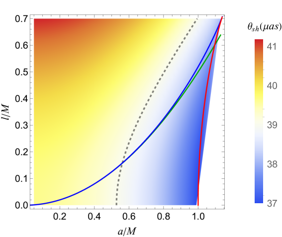
The EHT analysis suggested that, based on a priori known estimates for the mass and distance from stellar dynamics, the M87* shadow size is consistent within at a confidence interval of the size predicted from the Kerr black hole general relativistic-magneto-hydrodynamics (GRMHD) image (Akiyama et al. 2019a). However, several other studies altogether have not entirely precluded the possibility of non-Kerr black holes (Vincent et al. 2021; Mizuno et al. 2018). Using the M87* shadow angular size, constraints are placed on the second post-Newtonian metric coefficients, which were inaccessible in the earlier weak-field tests at the solar scale (Psaltis et al. 2020). Therefore, it is both legitimate and timely to test the viability of the LQRBH using the M87* black hole shadow observations. We determine the constraints on the LMRBH parameters using the deviation from the circularity of the black hole shadow and the angular diameter , to validate the suitability of the LMRBH as a candidate for the M87* black hole.
Let the shadow boundary be described by the polar coordinates () and the shadow has a center at (, ) with and . To assess the shadow deviation from a perfect circle, we define the dimensionless circularity deviation observable in terms of root-mean-square deviation from the average shadow radius as (Johannsen & Psaltis 2010; Johannsen 2013; Kumar et al. 2020b)
| (23) |
where is the shadow average radius defined as (Johannsen & Psaltis 2010)
| (24) |
with being the subtended polar angle and being the radial distance from the center (, ) of the shadow to any point () on the boundary. The variables connected with black holes, such as their mass , spin parameter , , or inclination angle , influence celestial coordinates, and as a result, also the observables and . To determine the black hole parameter values that are most likely to be observed, we compare our theoretical prediction to the EHT observation and use their result () to impose constraints on the LMRBH parameter space while accounting for the inclination angle with respect to the observational line of sight to be °(Craig Walker et al. 2018).
Next, the shadow angular diameter (Kumar & Ghosh 2020a; Kumar et al. 2021) is given by
| (25) |
where is the black hole shadow area,as defined in Equation 21, and is the distance of M87* from the Earth. In Figure 8, we demonstrate the LMRBH shadow angular diameter for ° as a function of and . The M87* black hole shadow angular diameter within the bound, , place a bound , whereas all values of are allowed. For , there is an upper limit on the value of which depends on the value of (see Figure 8). Thus, in this constrained parameter space, the M87* can be LMRBH spacetime. Since there is a number of possible parameter points (, ) within the confined parameter space, the LMRBH’s compatibility with the M87* observations demonstrates that they can be excellent candidates for astrophysical black holes. Circularity deviation is shown in Figure 10 for °. The M87* bound is satisfied by the LMRBH for the entire parameter space. This is because the rotating black hole shadows are nearly circular for small inclination angle.

V.2 Observational constraints from the EHT results of Sgr A*
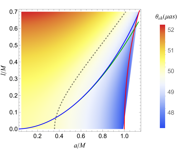
Based on the 2017 VLBI observing campaign at 1.3 mm wavelength, the EHT collaboration (Akiyama et al. 2022a; Akiyama et al. 2022b; Akiyama et al. 2022c; Akiyama et al. 2022d; Akiyama et al. 2022e; Akiyama et al. 2022f) published the shadow data for the Sgr A* black hole. Sgr A* black hole shadow images have advantages in testing the nature of an astrophysical black hole (i) Sgr A* probes a order of higher curvature than the M87* and (ii) independent prior estimates for mass-to-distance ratio are used for Sgr A*. The shadow images were created using a variety of imaging and modeling techniques, and they are astonishingly similar in features.

We will use the EHT bounds on the two observables, shadow angular diameter and Schwarzschild shadow deviation , to set constraints on the LMRBH parameters. We determine , which, in addition to other black hole parameters, relies on the mass , the distance of the black hole, LQG parameter , and inclination as depicted in Figure 9. We show that , i.e., within the region of the SgrA* shadow angular diameter, is satisfied for entire parameter space in the case of the LMRBH. Moreover, EHT used three independent imaging algorithms, namely, eht-imaging, SIMLI, DIFMAP, to determine the Sgr A* shadow’s average diameter as as. This range of angular diameter strongly constrains the parameters and at °. are the critical values of parameter represented by the red line in Figure 9 and is the maximum value of which depends on . For this constrained parameter range, the LMRBH shadows are consistent with the shadow of Sgr A*.
The Schwarzschild shadow deviation (), assesses the disparity between the shadow angular diameter of the LMRBH, , and the Schwarzschild shadow diameter, , and is given as (Akiyama et al. 2022e; Akiyama et al. 2022f)
| (26) |
For Kerr black hole with , the Schwarzschild shadow deviation lies at as the inclination varies from 0 to . EHT used the two separate priors for the Sgr A* angular size from the Keck and Very Large Telescope Interferometer (VLTI) observations to estimate the bounds on the fraction deviation observable (Akiyama et al. 2022e; Akiyama et al. 2022b)
| (27) |
Thus, modeling Sgr A* as an LMRBH, the entire parameter space in the case of the LMRBH is satisfied for inferred bound Keck (-0.14,0.05). On the other hand, the VLTI bound (-0.17,0.01), constrains the parameters () such that for Km), the allowed range of is . If , there is an upper bound on the value of which is not specific and depends on the value of ’’, for e.g., at , and at , ( Figure 11).
VI Conclusion
The scarcity of rotating black hole models in the LQG restricts the progress of testing LQG from observations, like the EHT observation of M87* and SgrA*. Furthermore, because of the rapidly growing astronomical observations of rotating black holes, starting from a nonrotating LQG seed metric (Equation (2)) and using a modified NJA generating technique we obtained a rotating LMRBH in an earlier work (Kumar et al. 2022). The LMRBH metric possesses a Kerr-like form and has several exciting properties (Kumar et al. 2022). It is nonsingular everywhere and reduces to the Kerr solution when the quantum effects are switched off (). Depending on values of parameters , the LMRBH can describe an NH, a generic regular black hole with Cauchy and event horizons (BH-II), or a black hole with one or three horizons (BH-I or BH-III).
Here, we are interested in the shadow and analyzed the LMRBH to find that the Hamilton-Jacobi equations are separable, resulting in null geodesic equations in the first-order differential form. In Figure 4, we depict the shadow cast by the LMRBH in the parameter space to find black hole shadow size increases monotonically, and the shape becomes more distorted with an increasing . For the given shadow observables, we have estimated parameters associated with the LMRBH by two popular methods, assuming that the observer is in the equatorial plane. We show that by using these shadow observables one can ultimately determine information about an LMRBH.
The supermassive black holes, M87* and Sgr A*, at the center of the Milky Way and M87, are a superior and realistic laboratory for testing the strong-field predictions of GR. The EHT collaboration has released the first horizon-scale images of both M87* and Sgr A*, and the EHT results are consistent with the prediction on the Kerr metric, and there is no evidence for any breach of the theory of GR. Here, we used the EHT observation of the black hole shadow in M87* and Sgr A* to place constraints on the deviation parameters associated with LMRBH.
To place constraints on the deviation parameter , we employ the angular size and asymmetry results of the EHT for the M87* black hole and the EHT bounds on the Sgr A* shadow angular diameter and Schwarzschild shadow deviation from the Sgr A* results. The allowed range of M87* angular shadow diameter within region, i.e., as is possible for the entire range of and . However, if , then there is an upper limit on which depends on . Likewise, we show that the Sgr A* shadow angular diameter within credible region, , is satisfied for the entire parameter space in the case of LMRBH. But, the EHT observation also employed three different techniques to determine that the shadow’s average measured angular diameter is within the range as which strongly constrains the parameters, such that and at °is allowed. Here, and are, respectively, the critical values of parameter represented by the red line in Figure 9 and maximum value of . Further, modeling Sgr A* as an LMRBH, the entire parameter space with the LMRBH is obeyed for the inferred Keck bound (-0.14,0.05). The VLTI bound (-0.17,0.01), constrains the parameters () such that for , the allowed range of is . For , the maximum value of depends on ’’. The shadow circularity deviation bound for M87* black hole allows the entire parameter space for LMRBH due to the low inclination angle, whereas the bound for Sgr A* is not available.
The main restriction of our proposition is that the LMRBH metric does not result from a direct loop quantization of the Kerr spacetime. However, we note that the existence of the region BH-I has similar features of nonrotating LQG black holes (1) (see the Penrose Diagram in Figure 2) and the LMRBH also provides the singularity resolution of Kerr black holes. Thus, it is pragmatic to expect that the LMRBH can capture some aspects of the effective regular spacetime description of LQG.
VII Acknowledgments
S.U.I and S.G.G. are supported by SERB-DST through project No. CRG/2021/005771. J.K. would like to thank CSIR for providing SRF. R.K.W. would like to thank the University of KwaZulu-Natal and the NRF for the postdoctoral research fellowship.
References
- Abdujabbarov et al. (2016) Abdujabbarov, A., Amir, M., Ahmedov, B., & Ghosh, S. G. 2016, Phys. Rev., D93, 104004, doi: 10.1103/PhysRevD.93.104004
- Abdujabbarov et al. (2015) Abdujabbarov, A. A., Rezzolla, L., & Ahmedov, B. J. 2015, Mon. Not. Roy. Astron. Soc., 454, 2423, doi: 10.1093/mnras/stv2079
- Akiyama et al. (2019a) Akiyama, K., et al. 2019a, Astrophys. J. Lett., 875, L1, doi: 10.3847/2041-8213/ab0ec7
- Akiyama et al. (2019b) —. 2019b, Astrophys. J. Lett., 875, L6, doi: 10.3847/2041-8213/ab1141
- Akiyama et al. (2019c) —. 2019c, Astrophys. J. Lett., 875, L3, doi: 10.3847/2041-8213/ab0c57
- Akiyama et al. (2019d) —. 2019d, Astrophys. J. Lett., 875, L5, doi: 10.3847/2041-8213/ab0f43
- Akiyama et al. (2019e) —. 2019e, Astrophys. J. Lett., 875, L4, doi: 10.3847/2041-8213/ab0e85
- Akiyama et al. (2019f) —. 2019f, Astrophys. J. Lett., 875, L2, doi: 10.3847/2041-8213/ab0c96
- Akiyama et al. (2022a) —. 2022a, Astrophys. J. Lett., 930, L15, doi: 10.3847/2041-8213/ac6736
- Akiyama et al. (2022b) —. 2022b, Astrophys. J. Lett., 930, L16, doi: 10.3847/2041-8213/ac6672
- Akiyama et al. (2022c) —. 2022c, Astrophys. J. Lett., 930, L13, doi: 10.3847/2041-8213/ac6675
- Akiyama et al. (2022d) —. 2022d, Astrophys. J. Lett., 930, L14, doi: 10.3847/2041-8213/ac6429
- Akiyama et al. (2022e) —. 2022e, Astrophys. J. Lett., 930, L12, doi: 10.3847/2041-8213/ac6674
- Akiyama et al. (2022f) —. 2022f, Astrophys. J. Lett., 930, L17, doi: 10.3847/2041-8213/ac6756
- Amarilla & Eiroa (2013) Amarilla, L., & Eiroa, E. F. 2013, Phys. Rev. D, 87, 044057, doi: 10.1103/PhysRevD.87.044057
- Amarilla et al. (2010) Amarilla, L., Eiroa, E. F., & Giribet, G. 2010, Phys. Rev. D, 81, 124045, doi: 10.1103/PhysRevD.81.124045
- Ashtekar & Bojowald (2006) Ashtekar, A., & Bojowald, M. 2006, Class. Quant. Grav., 23, 391, doi: 10.1088/0264-9381/23/2/008
- Ashtekar & Lewandowski (2004) Ashtekar, A., & Lewandowski, J. 2004, Class. Quant. Grav., 21, R53, doi: 10.1088/0264-9381/21/15/R01
- Ashtekar et al. (2006) Ashtekar, A., Pawlowski, T., & Singh, P. 2006, Phys. Rev. D, 74, 084003, doi: 10.1103/PhysRevD.74.084003
- Ashtekar et al. (2007) Ashtekar, A., Pawlowski, T., Singh, P., & Vandersloot, K. 2007, Phys. Rev. D, 75, 024035, doi: 10.1103/PhysRevD.75.024035
- Atamurotov et al. (2013) Atamurotov, F., Abdujabbarov, A., & Ahmedov, B. 2013, Phys. Rev. D, 88, 064004, doi: 10.1103/PhysRevD.88.064004
- Ayon-Beato & Garcia (1998) Ayon-Beato, E., & Garcia, A. 1998, Phys. Rev. Lett., 80, 5056, doi: 10.1103/PhysRevLett.80.5056
- Azreg-Aïnou (2014a) Azreg-Aïnou, M. 2014a, Phys. Rev. D, 90, 064041, doi: 10.1103/PhysRevD.90.064041
- Azreg-Aïnou (2014b) —. 2014b, Eur. Phys. J. C, 74, 2865, doi: 10.1140/epjc/s10052-014-2865-8
- Bardeen (1973) Bardeen, J. 1973, Black Holes, edited by C. DeWitt and BS DeWitt, Gordon and Breach, New York
- Bardeen (1968) Bardeen, J. M. 1968, in Conference Proceedings of GR5, 174, doi: 10.1142/S0218271815500200
- Barrabes & Frolov (1996) Barrabes, C., & Frolov, V. P. 1996, Phys. Rev. D, 53, 3215, doi: 10.1103/PhysRevD.53.3215
- Boehmer & Vandersloot (2007) Boehmer, C. G., & Vandersloot, K. 2007, Phys. Rev. D, 76, 104030, doi: 10.1103/PhysRevD.76.104030
- Boehmer & Vandersloot (2008) —. 2008, Phys. Rev. D, 78, 067501, doi: 10.1103/PhysRevD.78.067501
- Brahma et al. (2021) Brahma, S., Chen, C.-Y., & Yeom, D.-h. 2021, Phys. Rev. Lett., 126, 181301, doi: 10.1103/PhysRevLett.126.181301
- Bronnikov (2001) Bronnikov, K. A. 2001, Phys. Rev. D, 63, 044005, doi: 10.1103/PhysRevD.63.044005
- Bronnikov (2018) —. 2018, Particles, 1, 56, doi: 10.3390/particles1010005
- Bronnikov & Fabris (2006) Bronnikov, K. A., & Fabris, J. C. 2006, Phys. Rev. Lett., 96, 251101, doi: 10.1103/PhysRevLett.96.251101
- Bronnikov & Korolyov (2015) Bronnikov, K. A., & Korolyov, P. A. 2015, Grav. Cosmol., 21, 157, doi: 10.1134/S0202289315020024
- Bronnikov et al. (2003) Bronnikov, K. A., Melnikov, V. N., & Dehnen, H. 2003, Phys. Rev. D, 68, 024025, doi: 10.1103/PhysRevD.68.024025
- Bronnikov et al. (2007) —. 2007, Gen. Rel. Grav., 39, 973, doi: 10.1007/s10714-007-0430-6
- Bronnikov & Walia (2022) Bronnikov, K. A., & Walia, R. K. 2022, Phys. Rev. D, 105, 044039, doi: 10.1103/PhysRevD.105.044039
- Campiglia et al. (2008) Campiglia, M., Gambini, R., & Pullin, J. 2008, AIP Conf. Proc., 977, 52, doi: 10.1063/1.2902798
- Cardoso & Pani (2019) Cardoso, V., & Pani, P. 2019, Living Rev. Rel., 22, 4, doi: 10.1007/s41114-019-0020-4
- Carter (1968) Carter, B. 1968, Phys. Rev., 174, 1559, doi: 10.1103/PhysRev.174.1559
- Carter (1971) —. 1971, Phys. Rev. Lett., 26, 331, doi: 10.1103/PhysRevLett.26.331
- Chandrasekhar (1985) Chandrasekhar, S. 1985, The mathematical theory of black holes (Oxford: Oxford Univ. Press)
- Chen (2022) Chen, C.-Y. 2022, in Geometric Foundations of Gravity 2021. https://arxiv.org/abs/2207.03797
- Craig Walker et al. (2018) Craig Walker, R., Hardee, P. E., Davies, F. B., Ly, C., & Junor, W. 2018, Astrophys. J., 855, 128, doi: 10.3847/1538-4357/aaafcc
- Cunha & Herdeiro (2018) Cunha, P. V. P., & Herdeiro, C. A. R. 2018, Gen. Rel. Grav., 50, 42, doi: 10.1007/s10714-018-2361-9
- Cunningham & Bardeen (1973) Cunningham, C. T., & Bardeen, J. M. 1973, ApJ, 183, 237, doi: 10.1086/152223
- de Vries (2000) de Vries, A. 2000, Classical and Quantum Gravity, 17, 123, doi: 10.1088/0264-9381/17/1/309
- Dymnikova (1992) Dymnikova, I. 1992, Gen. Rel. Grav., 24, 235, doi: 10.1007/BF00760226
- Falcke et al. (2000) Falcke, H., Melia, F., & Agol, E. 2000, Astrophys. J. Lett., 528, L13, doi: 10.1086/312423
- Gambini & Pullin (2008) Gambini, R., & Pullin, J. 2008, Phys. Rev. Lett., 101, 161301, doi: 10.1103/PhysRevLett.101.161301
- Ghosh (2015) Ghosh, S. G. 2015, Eur. Phys. J. C, 75, 532, doi: 10.1140/epjc/s10052-015-3740-y
- Grenzebach et al. (2015) Grenzebach, A., Perlick, V., & Lämmerzahl, C. 2015, Int. J. Mod. Phys., D24, 1542024, doi: 10.1142/S0218271815420249
- Hawking & Ellis (1973) Hawking, S., & Ellis, G. 1973, Cambridge Univ. Press, 99, 124012, doi: 10.1103/PhysRevD.99.124012
- Hawking (1972) Hawking, S. W. 1972, Commun. Math. Phys., 25, 152, doi: 10.1007/BF01877517
- Hawking & Penrose (1970) Hawking, S. W., & Penrose, R. 1970, Proc. Roy. Soc. Lond. A, 314, 529, doi: 10.1098/rspa.1970.0021
- Hayward (2006) Hayward, S. A. 2006, Phys. Rev. Lett., 96, 031103, doi: 10.1103/PhysRevLett.96.031103
- Hioki & Maeda (2009) Hioki, K., & Maeda, K.-i. 2009, Phys. Rev. D, 80, 024042, doi: 10.1103/PhysRevD.80.024042
- Israel (1967) Israel, W. 1967, Phys. Rev., 164, 1776, doi: 10.1103/PhysRev.164.1776
- Israel (1968) —. 1968, Commun. Math. Phys., 8, 245, doi: 10.1007/BF01645859
- Jaroszynski & Kurpiewski (1997) Jaroszynski, M., & Kurpiewski, A. 1997, Astron. Astrophys., 326, 419. https://arxiv.org/abs/astro-ph/9705044
- Johannsen (2013) Johannsen, T. 2013, Astrophys. J., 777, 170, doi: 10.1088/0004-637X/777/2/170
- Johannsen & Psaltis (2010) Johannsen, T., & Psaltis, D. 2010, Astrophys. J., 718, 446, doi: 10.1088/0004-637X/718/1/446
- Johannsen & Psaltis (2011) —. 2011, Phys. Rev. D, 83, 124015, doi: 10.1103/PhysRevD.83.124015
- Kerr (1963a) Kerr, R. P. 1963a, Phys. Rev. Lett., 11, 237, doi: 10.1103/PhysRevLett.11.237
- Kerr (1963b) —. 1963b, Phys. Rev. Lett., 11, 237, doi: 10.1103/PhysRevLett.11.237
- Kramer et al. (2004) Kramer, M., Backer, D. C., Cordes, J. M., et al. 2004, New Astron. Rev., 48, 993, doi: 10.1016/j.newar.2004.09.020
- Kumar et al. (2022) Kumar, J., Islam, S. U., & ~Ghosh, S. 2022. https://arxiv.org/abs/2209.13562
- Kumar & Ghosh (2018) Kumar, R., & Ghosh, S. G. 2018, Eur. Phys. J. C, 78, 750, doi: 10.1140/epjc/s10052-018-6206-1
- Kumar & Ghosh (2020a) —. 2020a, JCAP, 07, 053, doi: 10.1088/1475-7516/2020/07/053
- Kumar & Ghosh (2020b) —. 2020b, Astrophys. J., 892, 78, doi: 10.3847/1538-4357/ab77b0
- Kumar et al. (2020a) Kumar, R., Ghosh, S. G., & Wang, A. 2020a, Phys. Rev. D, 101, 104001, doi: 10.1103/PhysRevD.101.104001
- Kumar et al. (2020b) Kumar, R., Kumar, A., & Ghosh, S. G. 2020b, Astrophys. J., 896, 89, doi: 10.3847/1538-4357/ab8c4a
- Kumar et al. (2021) Kumar, R., Singh, B. P., Ali, M. S., & Ghosh, S. G. 2021, Phys. Dark Univ., 34, 100881, doi: 10.1016/j.dark.2021.100881
- Kumar Walia (2022) Kumar Walia, R. 2022. https://arxiv.org/abs/2207.02106
- Lemos & Zanchin (2011) Lemos, J. P. S., & Zanchin, V. T. 2011, Phys. Rev. D, 83, 124005, doi: 10.1103/PhysRevD.83.124005
- Liu et al. (2020) Liu, C., Zhu, T., Wu, Q., et al. 2020, Phys. Rev. D, 101, 084001, doi: 10.1103/PhysRevD.101.084001
- Luminet (1979) Luminet, J. P. 1979, A&A, 75, 228
- Mishra et al. (2019) Mishra, A. K., Chakraborty, S., & Sarkar, S. 2019, Phys. Rev. D, 99, 104080, doi: 10.1103/PhysRevD.99.104080
- Mizuno et al. (2018) Mizuno, Y., Younsi, Z., Fromm, C. M., et al. 2018, Nature Astron., 2, 585, doi: 10.1038/s41550-018-0449-5
- Modesto (2006) Modesto, L. 2006, Class. Quant. Grav., 23, 5587, doi: 10.1088/0264-9381/23/18/006
- Modesto (2008) —. 2008, Adv. High Energy Phys., 2008, 459290, doi: 10.1155/2008/459290
- Modesto (2010) —. 2010, Int. J. Theor. Phys., 49, 1649, doi: 10.1007/s10773-010-0346-x
- Newman & Janis (1965) Newman, E. T., & Janis, A. I. 1965, J. Math. Phys., 6, 915, doi: 10.1063/1.1704350
- Peltola & Kunstatter (2009a) Peltola, A., & Kunstatter, G. 2009a, Phys. Rev. D, 80, 044031, doi: 10.1103/PhysRevD.80.044031
- Peltola & Kunstatter (2009b) —. 2009b, Phys. Rev. D, 79, 061501, doi: 10.1103/PhysRevD.79.061501
- Poisson & Israel (1988) Poisson, E., & Israel, W. 1988, Classical and Quantum Gravity, 5, L201, doi: 10.1088/0264-9381/5/12/002
- Psaltis et al. (2020) Psaltis, D., et al. 2020, Phys. Rev. Lett., 125, 141104, doi: 10.1103/PhysRevLett.125.141104
- Robinson (1975) Robinson, D. C. 1975, Phys. Rev. Lett., 34, 905, doi: 10.1103/PhysRevLett.34.905
- Shaikh (2019) Shaikh, R. 2019, Phys. Rev. D, 100, 024028, doi: 10.1103/PhysRevD.100.024028
- Shen et al. (2005) Shen, Z.-Q., Lo, K. Y., Liang, M. C., Ho, P. T. P., & Zhao, J. H. 2005, Nature, 438, 62, doi: 10.1038/nature04205
- Simpson & Visser (2019) Simpson, A., & Visser, M. 2019, JCAP, 02, 042, doi: 10.1088/1475-7516/2019/02/042
- Synge (1966) Synge, J. L. 1966, Monthly Notices of the Royal Astronomical Society, 131, 463, doi: 10.1093/mnras/131.3.463
- Takahashi (2004) Takahashi, R. 2004, J. Korean Phys. Soc., 45, S1808, doi: 10.1086/422403
- Tsupko (2017) Tsupko, O. Yu. 2017, Phys. Rev., D95, 104058, doi: 10.1103/PhysRevD.95.104058
- Vandersloot (2007) Vandersloot, K. 2007, Phys. Rev. D, 75, 023523, doi: 10.1103/PhysRevD.75.023523
- Vincent et al. (2021) Vincent, F. H., Wielgus, M., Abramowicz, M. A., et al. 2021, Astron. Astrophys., 646, A37, doi: 10.1051/0004-6361/202037787
- Wheeler (1963) Wheeler, J. A. 1963, Relativity, Groups and Topology (New York: Gordon and Breach)
- Yumoto et al. (2012) Yumoto, A., Nitta, D., Chiba, T., & Sugiyama, N. 2012, Phys. Rev. D, 86, 103001, doi: 10.1103/PhysRevD.86.103001
- Zaslavskii (2009) Zaslavskii, O. B. 2009, Phys. Rev. D, 80, 064034, doi: 10.1103/PhysRevD.80.064034