Computationally Light Spectrally Normalized Memory Neuron Network based Estimator for GPS-denied operation of Micro-UAV

The physics-based mathematical model of a typical UAV system is given below:

where $\hat{\boldsymbol{k}}=\left[0\ 0\ 1\right]^{T}$ is the unit vector along the $z-$axis, $\boldsymbol{x}\in\mathbb{R}^{3}$ is the position of the UAV with mass $m\in\mathbb{R}$ and moment of inertia $\boldsymbol{J}\in\mathbb{R}^{3\times 3}$, $\boldsymbol{v}\in\mathbb{R}^{3}$ is the linear velocity, $\boldsymbol{R}\in\mathbb{R}^{3\times 3}$ is the rotation matrix that converts a vector from the UAV-fixed body frame to the inertial frame, $\boldsymbol{\Omega}\in\mathbb{R}^{3}$ is the angular velocity of the UAV, $f_{t}\in\mathbb{R}$ is the input thrust vector and $\boldsymbol{\tau}\in\mathbb{R}^{3}$ is the input torque vector given by Eq. (1c) and (1) respectively. The quantities $\omega_{i}$ denotes the rotational velocity of the $i^{th}$ motor in (rad/s), $l$ denotes the arm length of the UAV, and the constants $K_{\omega},K_{d}$ denote the motor constant and the drag coefficient respectively. The operator $(.)^{\times}:\mathbb{R}^{3}\rightarrow\mathbb{R}^{3\times 3}$ is the hat operator that converts a vector to a skew-symmetric matrix. The quantities $\tilde{\boldsymbol{f}},\tilde{\boldsymbol{\tau}}$ represent the external complex aerodynamic forces and torques on the UAV that are mostly unknown or cannot be analytically modelled. In real world, the dynamics given by Eq. (1) are rudimentary and cannot be relied upon for estimating the UAV states due to presence of noise, model uncertainties and external disturbances.

In general, one can use billings theorem (Leontaritis and Billings 1985) to write the input-output model of a dynamical system as:

where $f(.)$ is an unknown nonlinear function, $n$ is the order of the system, $\boldsymbol{y}_{k}$ and $\boldsymbol{u}_{k}$ is the output of and input to the system respectively at time step $k$. Note that one can use a recurrent neural network to approximate the unknown nonlinear function using the current input and past output. It has been shown in the literature that the Memory Neuron Network (MNN) Sastry et al. 1994 is more efficient in approximating the dynamics accurately than other state-of-the-art recurrent neural networks (Rao and Sundaram 2021). The presence of uncertainty in thrust and the unknown disturbance influences the stability/reliability of prediction. The next section proposes a spectrally normalized MNN to learn the UAV model accurately.

The Spectrally Normalized Memory Neural Network (SN-MNN) contains fully connected network neurons (white circle) with its associated memory neurons (black solid circle). The unique nature of the connection between the Network Neurons and the Memory Neurons (see Fig.1) makes the network recurrent in nature. The network is parameterized by $\boldsymbol{\theta}=\left\{(^{1}\boldsymbol{W},^{1}\boldsymbol{Q}),\ldots,(^{L}\boldsymbol{W},^{L}\boldsymbol{Q})\right\}$, the weights corresponding to both the network neurons ($\boldsymbol{W}$) as well as the memory neurons ($\boldsymbol{Q}$). The left superscript denotes the layer number. Thus, the output of SN-MNN to an input $\boldsymbol{p}$ can be compactly represented as:

where $\phi(.)$ denotes the activation function and ${}^{l}\boldsymbol{r}$ denotes the output of the memory neurons present in the $l^{th}$ layer. The recurrence relationship between the memory neurons and the network neurons can be represented as:

where ${}^{l}\boldsymbol{n}=\phi(.)$ is the output of the activation function in the $l$^th layer and ${}^{l}\boldsymbol{\alpha}$ is the weight of the feedback connections between the network and the memory neurons in the $l$^th layer (see Fig. 1).

The Lipschitz constant $\gamma$ of a real valued function $f:\mathbb{R}^{n}\rightarrow\mathbb{R}$ is defined mathematically as:

The Lipschitz constant of a differentiable function is the maximum spectral norm of its Jacobian over the function’s domain: $\gamma=\text{sup}_{\boldsymbol{p}}\ \rho(\nabla f(\boldsymbol{p}))$, where $\rho(\boldsymbol{A})$ denotes the spectral norm of the matrix $\boldsymbol{A}$ which is defined as the square root of maximum eigenvalue of the matrix $A^{H}A$. As demonstrated in (Shi et al. 2019), it is essential to limit the Lipschitz constant of a neural network to ensure stable reliable prediction performance that is comparable with the actual dynamics of the UAV. The following Theorem guarantees the Lipschitz constant of the SN-MNN:

For training the network, the modified backpropagation approach as described in (Sastry et al. 1994) is used, with the following cost function being minimized during training at every time step:

where the input $\boldsymbol{p}_{k}=\left[\boldsymbol{y}_{k-1}^{T}\ \ \overline{\boldsymbol{\omega}}_{k}^{T}\ \ \boldsymbol{\Theta}_{k}^{T}\right]^{T}$ consists of the previous position of the UAV $\boldsymbol{y}_{k-1}\in\mathbb{R}^{3}$, the roll-pitch-yaw orientation of the UAV $\boldsymbol{\Theta}_{k}\in\mathbb{R}^{3}$ and the current normalized motor RPM $\boldsymbol{\overline{\omega}}_{k}\in\mathbb{R}^{4}$. The training process of the network is illustrated in Fig. 1. Let $\boldsymbol{e}$ be the error vector. Due to the constraint of Eq. (9b), the update rules for $\boldsymbol{W}$ and $\boldsymbol{Q}$ are as follows:

More details of the update rule derivation are provided in the supplementary material Rao 2022.

The network predicts the position of the UAV based on the rotor RPM input. This position estimate can be used during state fusion typically performed by an onboard Extended Kalman Filter (EKF), in addition to the state information provided by other peripheral sensors like IMU, compass, magnetometer, airflow sensor etc. In this work, the position estimates given by the network are converted to GPS coordinates $\boldsymbol{\zeta}_{k}$, also known as geodetic coordinates (latitude $\phi$, longitude $\lambda$, altitude $\mathfrak{z}$) and transformed GPS coordinates are used by the EKF for state estimation. This is illustrated in Fig. 2 and Fig. 3. Since many flight controllers offer out-of-box support for real-time GPS fusion, it has been adopted in this paper. Moreover, ground control software utilises GPS coordinates to visualise the UAV path and monitor its itinerary and the course of navigation.

The ENU coordinates must first be converted to the ECEF (Earth-Center, Earth-Fixed) coordinate system before converting it to the GPS coordinates. Detailed information on converting the ENU coordinates to the GPS coordinates (via ECEF coordinates) is provided in the supplementary material Rao 2022. However, the following equations summarize the conversion to GPS coordinates:

where the parameters $\kappa$ and $D$ can be calculated by the set of equations given in the supplementary material Rao 2022. This process is briefly summarized in Fig. 3.

The experimental setup consists of an outdoor RTK GPS facility (Here+ RTK Base with Here3 RTK GPS) with base station survey-in accuracy of 1m (relative accuracy of 10cm) and a custom-built micro-UAV (generic 250 racer frame) with the Pixhawk 4 Flight Controller that runs on PX4 firmware. The RTK facility and a micro-UAV operating in the facility are shown in Fig. 4. The drone weighs about 1.1 Kg, with a RaspberryPi 4 onboard computer. The onboard sensors include an accelerometer, gyroscope, barometer and a compass, all present inside the flight controller. In addition to this, the Velox V2 1950KV T-motors are used with a 5-inch 3 blade propeller configuration. The data is collected on a typical day with mild steady wind influences.

For training the network, experimental data is collected from the test facility. The states of the UAV and the $4$ rotor rpm are logged for multiple flights. The DShot protocol is used by the F55A electronic speed controller (ESC), which measures the rotor RPM values based on the back-EMF from the motor. The flight data mainly consists of random trajectories performed manually and certain square and circular trajectories performed autonomously by the UAV. These flights ensure that all possible UAV configuration in its state-space are captured.

Next, a common sampling frequency is chosen to sample the data corresponding to different sensors (IMU, Barometer, Compass, RPM data and the RTK GPS position information). The RPM values are normalized based on the motor’s maximum RPM. The final data consists of $12$ columns: one common timestamp for all other columns, $4$ normalized rotor rpm (from ESC), position, and quaternion orientation of the UAV. The entire data is then split into training and testing data in the ratio of 3:2.

The SN-MNN is trained to predict the one-step-ahead position of the UAV, with the current UAV position $\boldsymbol{y}_{k}\in\mathbb{R}^{3}$, orientation (Euler angles) $\boldsymbol{q}_{k}\in\mathbb{R}^{4}$ and the normalized rotor RPM $\overline{\boldsymbol{\omega}}_{k}\in\mathbb{R}^{4}$ as the input to the network. Hence, the selected architecture of SN-MNN is: $11$ input neurons, $100$ hidden neurons and $3$ output neurons. The network neurons in the hidden layer uses $tanh(.)$ activation and the network neurons in output layer employ linear activation function. The network is implemented in Python using Numpy Library. The network is trained for a total of $50$ epochs. The variation of the squared loss during training is shown in Fig. 5 for with and without spectral normalization.

The output of the network for the entire test data (combined into one) is shown in Fig. 5. The RMSE for the entire position prediction is about $5.84cm$, whereas, for the network without spectral normalization, the RMSE error is about $50cm$, thus justifying the requirement for a spectrally normalized network. It can be seen from Fig. 5 that the network has successfully learned the UAV dynamics accurately. The value of the Lipschitz constant $\gamma$ (here $\gamma=1$) of the network plays an important role in the stabilization of the network during the training process. It also determines ”how fast” the network output can vary: For e.g. if the UAV is mostly hovering and making slow movements, the Lipschitz constant can be set to a low value. If the UAV is performing aggressive sharp maneuvers frequently, then the Lipschitz constant of the network must be set to a high value. In this paper, the trajectory data is collected for a UAV that mostly cruises and exhibits slow maneuvers.

Once the predicted position $\boldsymbol{y}_{k}$ is obtained from the SN-MNN, the GPS geodetic vector $\boldsymbol{\zeta}_{k}$ is calculated from Eq. 12, which is then given to the EKF for state fusion along with other state information like orientation, linear velocities (IMU) and UAV heading (compass). This is illustrated in Fig. 3. An instance of the PX4-ECL library is started on the onboard Raspberry-pi computer, and the state estimation process using the position predicted by the SN-MNN starts parallelly with the state-estimation process on the PX4-Autopilot that uses the GPS for the UAV flight. This is done to facilitate a real-time comparison of the position obtained (after state fusion) from the proposed algorithm vs. the position obtained (after state fusion) using an RTK GPS.

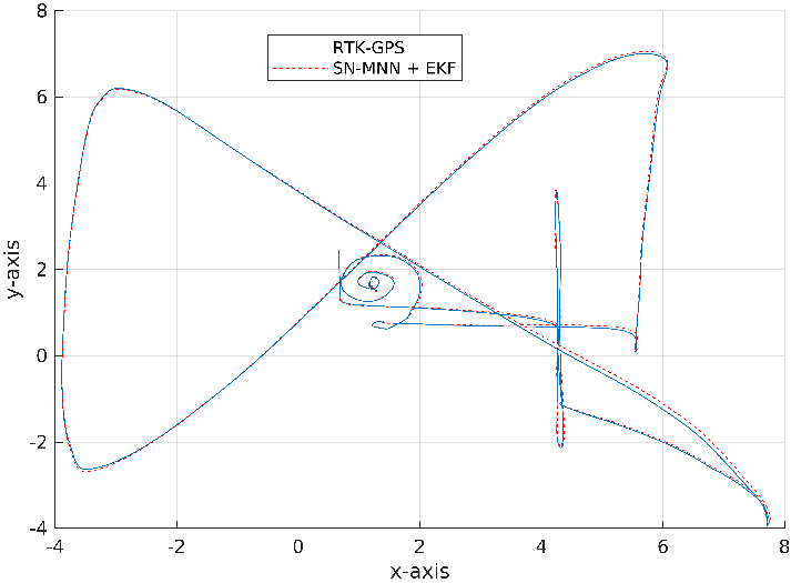
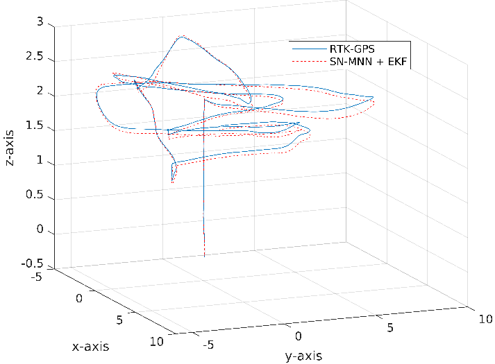
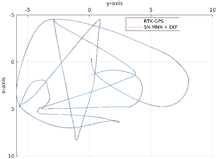
The outputs for two sample test trajectories are shown in Fig. 6 and Fig. 7 after the PX4-ECL state fusion is performed. It must be noted that the GPS fusion only affects the position and linear velocity of the UAV, not its rotational components. The RMSE between the estimated positions and the actual positions of the UAV for the course of the entire test flight duration (all test trajectories combined) is around $6cm$, whereas, for the network without spectral normalization, the RMSE is around $55cm$. Further, Table 1 shows a comparison with two state-of-art methods, namely the Visual Inertial Navigation System (VINS) and the Visual Inertial Odometry (VIO). The RMSE reported by these methods is compared along with the proposed method in this work. It can be seen that the RMSE reduces by about $60\%$ for VINS-mono(Qin et al. 2018) and about $40\%$ for VIO(Loianno et al. 2016). Further, the algorithm is computationally light, as one has to implement only the trained feedforward SN-MNN model. This implementation can be done directly on the flight controller, requiring no additional onboard computer. Thus, from the above results, it can be concluded that the proposed algorithm can be used to estimate the UAV states from the rotor RPM reliably.

References

- Al-Sharman et al. (2019) Mohammad K Al-Sharman, Yahya Zweiri, Mohammad Abdel Kareem Jaradat, Raghad Al-Husari, Dongming Gan, and Lakmal D Seneviratne. Deep-learning-based neural network training for state estimation enhancement: Application to attitude estimation. IEEE Transactions on Instrumentation and Measurement, 69(1):24–34, 2019.
- Assad et al. (2020) Ammar Assad, Wassim Khalaf, and Ibrahim Chouaib. Radial basis function kalman filter for attitude estimation in GPS-denied environment. IET Radar, Sonar & Navigation, 14(5):736–746, 2020.
- Balamurugan et al. (2016) G Balamurugan, J Valarmathi, and VPS Naidu. Survey on uav navigation in gps denied environments. In 2016 International conference on signal processing, communication, power and embedded system (SCOPES), pages 198–204. IEEE, 2016.
- Forster et al. (2013) Christian Forster, Deon Sabatta, Roland Siegwart, and Davide Scaramuzza. RFID-based hybrid metric-topological slam for GPS-denied environments. In 2013 IEEE International Conference on Robotics and Automation, pages 5228–5234. IEEE, 2013.
- Geodetic System (2017) Geodetic System. Geodetic system — the GIS encyclopedia, 2017. URL http://wiki.gis.com/wiki/index.php/Geodetic_system. [Online; modified 13-February-2017].
- Karney (2015) Charles Karney. Geographiclib. online at http://geographiclib. sourceforge. net, 2015.
- Khattak et al. (2019) Shehryar Khattak, Frank Mascarich, Tung Dang, Christos Papachristos, and Kostas Alexis. Robust thermal-inertial localization for aerial robots: A case for direct methods. In 2019 International Conference on Unmanned Aircraft Systems (ICUAS), pages 1061–1068. IEEE, 2019.
- Kim et al. (2005) Jonghyuk Kim, Salah Sukkarieh, et al. 6dof slam aided GNSS/INS navigation in GNSS denied and unknown environments. Positioning, 1(09), 2005.
- Leontaritis and Billings (1985) IJ Leontaritis and Stephen A Billings. Input-output parametric models for non-linear systems part i: deterministic non-linear systems. International journal of control, 41(2):303–328, 1985.
- Lindstrom et al. (2020) Colton Lindstrom, Randall Christensen, and Jacob Gunther. An investigation of GPS-denied navigation using airborne radar telemetry. In 2020 IEEE/ION Position, Location and Navigation Symposium (PLANS), pages 168–176, 2020.
- Loianno et al. (2016) Giuseppe Loianno, Michael Watterson, and Vijay Kumar. Visual inertial odometry for quadrotors on se (3). In 2016 IEEE International Conference on Robotics and Automation (ICRA), pages 1544–1551. IEEE, 2016.
- Majdik et al. (2015) András L Majdik, Damiano Verda, Yves Albers-Schoenberg, and Davide Scaramuzza. Air-ground matching: Appearance-based GPS-denied urban localization of micro aerial vehicles. Journal of Field Robotics, 32(7):1015–1039, 2015.
- Mebarki and Lippiello (2014) Rafik Mebarki and Vincenzo Lippiello. Image moments-based velocity estimation of UAVs in GPS denied environments. In 2014 IEEE International Symposium on Safety, Security, and Rescue Robotics (2014), pages 1–6. IEEE, 2014.
- Mohta et al. (2018) Kartik Mohta, Michael Watterson, Yash Mulgaonkar, Sikang Liu, Chao Qu, Anurag Makineni, Kelsey Saulnier, Ke Sun, Alex Zhu, Jeffrey Delmerico, et al. Fast, autonomous flight in GPS-denied and cluttered environments. Journal of Field Robotics, 35(1):101–120, 2018.
- Qin et al. (2018) Tong Qin, Peiliang Li, and Shaojie Shen. Vins-mono: A robust and versatile monocular visual-inertial state estimator. IEEE Transactions on Robotics, 34(4):1004–1020, 2018. 10.1109/TRO.2018.2853729.
- Rao (2022) Nishanth Rao. Supplementary Material for this paper. https://drive.google.com/drive/folders/1JhRFm5EMxU0DQkKRFG7VsiZ9myiokVK_?usp=sharing, 2022. [Online Google drive].
- Rao and Sundaram (2021) Nishanth Rao and Suresh Sundaram. Spatio-temporal look-ahead trajectory prediction using memory neural network. In 2021 International Joint Conference on Neural Networks (IJCNN), pages 1–8, 2021. 10.1109/IJCNN52387.2021.9534209.
- Riseborough and Team (2016) Paul Riseborough and Team. PX4 Estimation and Control Library. https://github.com/PX4/PX4-ECL, 2016.
- Sastry et al. (1994) PS Sastry, G Santharam, and KP Unnikrishnan. Memory neuron networks for identification and control of dynamical systems. IEEE transactions on neural networks, 5(2):306–319, 1994.
- Scaramuzza et al. (2014) Davide Scaramuzza, Michael C Achtelik, Lefteris Doitsidis, Fraundorfer Friedrich, Elias Kosmatopoulos, Agostino Martinelli, Markus W Achtelik, Margarita Chli, Savvas Chatzichristofis, Laurent Kneip, et al. Vision-controlled micro flying robots: from system design to autonomous navigation and mapping in GPS-denied environments. IEEE Robotics & Automation Magazine, 21(3):26–40, 2014.
- Shi et al. (2019) Guanya Shi, Xichen Shi, Michael O’Connell, Rose Yu, Kamyar Azizzadenesheli, Animashree Anandkumar, Yisong Yue, and Soon-Jo Chung. Neural lander: Stable drone landing control using learned dynamics. In 2019 International Conference on Robotics and Automation (ICRA), pages 9784–9790. IEEE, 2019.
- Tsai and Zhuang (2016) Shang-En Tsai and Shih-Hsien Zhuang. Optical flow sensor integrated navigation system for quadrotor in GPS-denied environment. In 2016 International Conference on Robotics and Automation Engineering (ICRAE), pages 87–91. IEEE, 2016.
- Urzua et al. (2017) Sarquis Urzua, Rodrigo Munguía, and Antoni Grau. Vision-based slam system for MAVs in GPS-denied environments. International Journal of Micro Air Vehicles, 9(4):283–296, 2017.
- Vermeille (2002) Hugues Vermeille. Direct transformation from geocentric coordinates to geodetic coordinates. Journal of Geodesy, 76(8):451–454, 2002.
- Vermeille (2011) Hugues Vermeille. An analytical method to transform geocentric into geodetic coordinates. Journal of Geodesy, 85(2):105–117, 2011.
- Zahran et al. (2019) Shady Zahran, Adel Moussa, and Naser El-Sheimy. Enhanced drone navigation in GNSS denied environment using VDM and hall effect sensor. ISPRS International Journal of Geo-Information, 8(4):169, 2019.
- Zhu et al. (2020) Kai Zhu, Xuan Guo, Changhui Jiang, Yujingyang Xue, Yuanjun Li, Lin Han, and Yuwei Chen. MIMU/odometer fusion with state constraints for vehicle positioning during beidou signal outage: Testing and results. Sensors, 20(8):2302, 2020.