跳到论文正文
W Papers独立论文阅读器 arXiv:2211.06344 论文正文 计算阅读时间 · 0%
引用这篇论文根据当前论文元数据生成,正式投稿前建议核对。


License: arXiv.org perpetual non-exclusive license
arXiv:2211.06344v3 [cs.IT] 01 May 2023

Simultaneous Active and Passive Information Transfer for RIS-Aided MIMO Systems: Iterative Decoding and Evolution Analysis

Affiliation: Wenjun Jiang, , and Xiaojun Yuan,  Thanks:  This work has been accepted for publication in IEEE Transactions on Signal Processing, 2023. W. Jiang and X. Yuan are with the National Key Lab. on Wireless Communi., University of Electronic Sci. and Tech. of China, Chengdu, China. (e-mail:wjjiang@std.uestc.edu.cn; xjyuan@uestc.edu.cn).
Abstract

This paper investigates the potential of reconfigurable intelligent surface (RIS) for passive information transfer in a RIS-aided multiple-input multiple-output (MIMO) system. We propose a novel simultaneous active and passive information transfer (SAPIT) scheme. In SAPIT, the transmitter (Tx) and the RIS deliver information simultaneously, where the RIS information is carried through the RIS phase shifts embedded in reflected signals. We introduce the coded modulation technique at the Tx and the RIS. The main challenge of the SAPIT scheme is to simultaneously detect the Tx signals and the RIS phase coefficients at the receiver. To address this challenge, we introduce appropriate auxiliary variables to convert the original signal model into two linear models with respect to the Tx signals and one entry-by-entry bilinear model with respect to the RIS phase coefficients. With this auxiliary signal model, we develop a message-passing-based receiver algorithm. Furthermore, we analyze the fundamental performance limit of the proposed SAPIT-MIMO transceiver. Notably, we establish state evolution to predict the receiver performance in a large-size system. We further analyze the achievable rates of the Tx and the RIS, which provides insight into the code design for sum-rate maximization. Numerical results validate our analysis and show that the SAPIT scheme outperforms the passive beamforming counterpart in achievable sum rate of the Tx and the RIS.

Index Terms: 
Reconfigurable intelligent surface, multiple-input multiple-output, active and passive information transfer, message passing, state evolution.

I Introduction

Reconfigurable intelligent surface (RIS), a.k.a. intelligent reflecting surface (IRS), has been envisioned as an emerging technology to empower sixth-generation (6G) wireless communications [1, 2, 3]. As a passive device, RIS can be deployed without requiring radio-frequency (RF) modules such as power amplifiers and analog-to-digital converters. A typical RIS consists of an array of reflecting elements, where each element can induce a phase shift to the incident electromagnetic wave in a nearly passive manner. As such, the RIS was utilized as a passive beamformer to shape the wireless propagation channel [4, 5, 6]. It was shown that through a collaborative optimization over the RIS phase shifts, RIS can provide a highly reliable link with the power gain quadratic to the number of the reflecting elements [7]. Yet, passive beamforming is not necessarily the most spectrum-efficient way of exploiting the ultimate potential of RIS.

Recently, the use of RIS for passive information transfer has been studied in [8, 9, 10, 11, 12, 13, 14, 15, 16]. As a pioneering attempt, the work in [8] studied passive beamforming and information transfer (PBIT) in a single-input multiple-output (SIMO) system, where the RIS delivers information through the random on/off state of each RIS element, referred to as on-off reflection modulation. This idea of PBIT was extended to the multiple-input multiple-output (MIMO) system in [9], and a turbo message-passing (TMP) algorithm was proposed to alternatively detect the transmitter (Tx) signals and the RIS on/off states. The authors in [13] pointed out that the on-off reflection modulation at every RIS element leads to signal-to-noise-ratio (SNR) fluctuation. They alleviated this problem by designing appropriate reflection patterns of the RIS elements. Ref. [14] further proposed quadrature reflection modulation to switch on all RIS elements, which avoids the SNR fluctuation problem. The authors in [15] proposed a joint design of the RIS reflection patterns and the Tx signals for bit error rate (BER) minimization. In [16], the authors built a RIS prototype that passively transfers information to multiple receivers in an indoor Wi-Fi scenario. However, a common problem in [10, 16, 15, 11, 12, 13, 14] is that nn-bit modulation of the RIS requires the use of 2n2^{n} different reflection patterns, which causes a high cost in reflection pattern design and related pattern detection, especially when the RIS operates at a high transmission rate.

More recently, much research interest has been attracted to analyze the information-theoretic performance limit of simultaneous active and passive information transfer (SAPIT), where the Tx and the RIS deliver information simultaneously. In [17], the authors studied SAPIT in the RIS-aided SIMO system and pointed out that joint channel encoding at the Tx and the RIS achieves a much higher achievable rate than the counterpart passive beamforming scheme. Ref. [18] further extended the analysis to the RIS-aided MIMO system, and showed that passive information transfer outperforms passive beamforming in multiplexing gain. However, due to the high-dimensional integration in the computation of achievable rates, ref. [17] considered a small-scale system with a single Tx antenna and a few number of RIS elements, and ref. [18] considered asymptotic rate analysis in the high SNR regime.

The study of RIS for passive information transfer is still in an infancy stage. Particularly, how to fully exploit the potential of RIS for passive information transfer with affordable complexity remains an open challenge. To address this challenge, we propose a new SAPIT scheme for the RIS-aided MIMO system. We first introduce coded modulation at the Tx and the RIS to relieve the burden of the reflection pattern designs as in [10, 16, 15, 11, 12, 13, 14]. With coded modulation, every RIS element can deliver information by modulation techniques, e.g., phase shift keying (PSK) modulation, and the information is encoded to ensure reliable transmission. Then, the main difficulty of the SAPIT scheme is to simultaneously retrieve the information from the Tx and the information from the RIS. This is a bilinear detection problem by noting that the received signal is a bilinear function of the Tx signal and the RIS phase coefficients. We introduce appropriate auxiliary variables to convert the original signal model into three parts, namely, two linear models of the Tx signals, and one entry-by-entry bilinear model of the RIS phase coefficients. Based on this auxiliary system, we formulate the bilinear detection problem into a Bayesian inference problem, and then develop a message-passing algorithm. In the proposed algorithm, inferring the Tx signals from the two linear models is achieved by employing the approximate message passing (AMP) tool [19, 20, 21]. More importantly, due to the fact that the entry-by-entry bilinear model of the RIS phase coefficients is among the simplest bilinear models, inferring the RIS phase coefficients is directly obtained through standard message passing.

We further analyze the fundamental performance limit of the SAPIT-MIMO transceiver. We show that in a large-size system, the receiver performance can be accurately characterized by state evolution (SE). A key finding in the SE is that in each message-passing iteration, the equivalent channels experienced by the Tx signals can be treated as additive Gaussian white noise (AWGN) channels and those experienced by the RIS phase coefficients can be treated as Rayleigh fading channels in the large-system limit. The equivalence to AWGN model is due to the use of the two linear models, which is similar to the finding in the SE analysis of AMP [22]. The equivalence to Rayleigh fading model is due to the use of the entry-by-entry bilinear model. Based on the SE, we derive the achievable rates of the Tx and the RIS based on the mutual information and minimum mean-square error relationship [23]. Particularly, we interpret the message-passing process as the iteration between a bilinear detector and two decoders, and the maximal achievable sum rate is obtained when the transfer functions of the detector and the two decoders are matched. Simulations validate that SE results match well with numerical results, and show that the proposed SAPIT scheme significantly outperforms the counterpart passive beamforming scheme in terms of achievable sum rate.

The main contributions of this paper are summarized below:

  • •

    We propose a novel SAPIT scheme in the RIS-aided MIMO system, where every RIS element can passively deliver information by the randomness of the phase coefficients. We introduce the coded modulation technique to relieve the burden of the existing reflection pattern designs.

  • •

    We show that the SAPIT-MIMO system model is equivalent to two linear models of the Tx signals plus one entry-by-entry bilinear model of the RIS phase coefficients. We then formulate the bilinear detection problem into a Bayesian inference problem, and develop a message-passing-based detection algorithm.

  • •

    We analyze the fundamental performance limit of the proposed SAPIT-MIMO transceiver. Particularly, we establish the SE to accurately characterize the performance of the proposed massage-passing algorithm in the large-size system. Based on the SE, we derive the achievable-rate bounds of the Tx and the RIS.

Passive beamforming aims to enhance the channel quality of the Tx by adjusting RIS reflection coefficients, while SAPIT aims to maximize the passive information transfer capability of the RIS by designing RIS reflection patterns. The values of the RIS reflection coefficients are typically known to the receiver in passive beamforming, but unknown to the receiver in SAPIT. PBIT can be regarded as a combination of passive beamforming and SAPIT, where the RIS reflection coefficients are partially optimized to enhance the channel quality of the main link, and partially kept random for passive information transfer. By adjusting the amount of “randomness” in the reflection coefficients, there is generally a trade-off between the passive beamforming gain and the information delivery capability of the RIS. We show that, as two extremes of this trade-off, SAPIT can significantly outperform passive beamforming in terms of achievable sum rate of the overall scheme.

Organization: In Sec. II, we establish the SAPIT scheme in the RIS-aided MIMO system. In Sec. III, we formulate the receiver design problem into a Bayesian inference problem, and develop a message-passing algorithm. In Sec. IV, we develop state evolution to predict the algorithm performance and analyze the achievable rates of the Tx and the RIS. In Sec. V, we present extensive numerical results. In Sec. VI, we conclude this paper.

Notation: We use bold capital letters (e.g., 𝐗\mathbf{X}) for matrices and bold lowercase letters (e.g., 𝐱\mathbf{x}) for vectors. (⋅)T(\cdot)^{T}, (⋅)∗(\cdot)^{*}, and (⋅)H(\cdot)^{H} denote the transpose, the conjugate, and the conjugate transpose, respectively. The cardinality of a set 𝒳\mathcal{X} is denoted as |𝒳||\mathcal{X}|. We use diag⁡(𝐱){\rm diag}(\mathbf{x}) for the diagonal matrix created from vector 𝐱\mathbf{x}. ‖𝐗‖F||\mathbf{X}||_{F} and ‖𝐱‖2||\mathbf{x}||_{2} denote the Frobenius norm of matrix 𝐗\mathbf{X} and the l2l_{2} norm of vector 𝐱\mathbf{x}, respectively. 𝐱1≺𝐱2\mathbf{x}_{1}\prec\mathbf{x}_{2} represents that every coordinate of 𝐱1\mathbf{x}_{1} is less than that of 𝐱2\mathbf{x}_{2}. δ⁡(⋅)\delta(\cdot) denotes the Dirac delta function. Matrix 𝐈\mathbf{I} denotes the identity matrix with an appropriate size. For a random vector 𝐱\mathbf{x}, we denote its probability density function (pdf) by p⁡(𝐱)p(\mathbf{x}). The pdf of a complex Gaussian random vector 𝐱∈ℂN\mathbf{x}\in\mathbb{C}^{N} with mean 𝐦\mathbf{m} and covariance 𝐂\mathbf{C} is denoted by 𝒞​𝒩​(𝐱,𝐦,𝐂)=exp⁡(−(𝐱−𝐦)H​𝐂−1​(𝐱−𝐦))/(πN​|𝐂|)\mathcal{CN}(\mathbf{x};\mathbf{m},\mathbf{C})={\rm exp}(-(\mathbf{x}-\mathbf{m})^{H}\mathbf{C}^{-1}(\mathbf{x}-\mathbf{m}))/(\pi^{N}|\mathbf{C}|). 𝔼⁡[⋅]\mathbb{E}[\cdot] and var​(⋅)\text{var}(\cdot) denote expectation and variance operators.

II System Model

II-A Channel Model

As illustrated in Fig. 1, we consider the RIS-aided MIMO system consisting of a KK-antenna transmitter (Tx), an MM-antenna receiver (Rx), and an NN-element RIS. Denote by 𝐅∈ℂN×K\mathbf{F}\in\mathbb{C}^{N\times K}, 𝐆∈ℂM×N\mathbf{G}\in\mathbb{C}^{M\times N}, and 𝐇∈ℂM×K\mathbf{H}\in\mathbb{C}^{M\times K} respectively the baseband channel matrices from the Tx to the RIS, from the RIS to the Rx, and from the Tx to the Rx. We assume that the channel is block-fading, i.e., the channel matrices 𝐅\mathbf{F}, 𝐆\mathbf{G}, and 𝐇\mathbf{H} remain constant in a transmission block. Without loss of generality, each transmission block consists of QQ sub-blocks, and each sub-block is divided into T≥1T\geq 1 time slots. The Tx symbols are changed from time-slot to time-slot while the RIS phases are changed from sub-block to sub-block. In practice, the choice of TT is determined by the speed limit of the phase adjustment of the RIS controller [24]. We ignore the mutual coupling between RIS elements. The signals reflected by the RIS two or more times are also ignored due to severe path loss.11 1 We note that mutual coupling and multi-reflection generally lead to more complicated physical models than (1) [25, 26]. The corresponding SAPIT design for those models is a very interesting research topic, but is left for future work. Then, the received signal model in the tt-th time slot of the qq-th sub-block is expressed as

𝐲q​t\displaystyle\quad\mathbf{y}_{qt} =(𝐆​diag​(𝐬q)​𝐅+𝐇)​𝐱q​t+𝐰q​t,∀q,t,\displaystyle=\left(\mathbf{G}\text{diag}(\mathbf{s}_{q})\mathbf{F}+\mathbf{H}\right)\mathbf{x}_{qt}+\mathbf{w}_{qt},~\forall q,t, (1)

where 𝐲q​t=[yq​t​1,…,yq​t​M]T∈ℂM\mathbf{y}_{qt}=[y_{qt1},...,y_{qtM}]^{T}\in\mathbb{C}^{M} is the received signal vector in the tt-th time slot of the qq-th sub-block; 𝐬q=[sq​1,…,sq​N]T∈ℂN\mathbf{s}_{q}=[s_{q1},...,s_{qN}]^{T}\in\mathbb{C}^{N} and 𝐱q​t=[𝐱q​t​1,…,𝐱q​t​K]T∈ℂK\mathbf{x}_{qt}=[\mathbf{x}_{qt1},...,\mathbf{x}_{qtK}]^{T}\in\mathbb{C}^{K} are the reflecting phase coefficient vector of the RIS and the signal vector of the Tx, respectively; 𝐰q​t∈ℂM\mathbf{w}_{qt}\in\mathbb{C}^{M} is an additive white Gaussian noise (AWGN) vector with elements independently drawn from 𝒞​𝒩​(0,σw2)\mathcal{CN}(0,\sigma_{w}^{2}). Each element of 𝐬q\mathbf{s}_{q} is constrained on a constellation 𝒮={ej​θ1,…,ej​θ|𝒮|}\mathcal{S}=\{e^{j\theta_{1}},...,e^{j\theta_{|\mathcal{S}|}}\}, where θi,i=1,…,|𝒮|\theta_{i},i=1,...,|\mathcal{S}| are the adjustable phase angles of the RIS controller. The constant modulus constraints of the RIS coefficients are naturally satisfied by our design. We assume that each element of 𝐱q​t\mathbf{x}_{qt} is constrained on a constellation 𝒳\mathcal{X} with cardinality |𝒳||\mathcal{X}| and unit average power. This assumption does not lose any generality since we can design the constellation points of 𝒳\mathcal{X} to approach any signal shaping (e.g., Gaussian signaling). We also assume that channel state information (CSI) is perfectly known. In practice, CSI can be acquired, e.g., by using the techniques in [27] and [28].

Fig. 1: Illustration of the RIS-aided MIMO system consisting of a KK-antenna Tx, an MM-antenna Rx, and an NN-element RIS. Information are delivered by both the RIS and the Tx.

II-B Transmitter and RIS Design

In this subsection, we describe the transmitter and RIS design for SAPIT. As shown in Fig. 1, we introduce the Tx encoder and the RIS encoder for reliable transmission. Denote by 𝒞x\mathcal{C}_{x} and 𝒞s\mathcal{C}_{s} the codebooks adopted at the Tx and the RIS encoder, respectively. At the Tx, a codeword matrix 𝐗=[𝐱11,…,𝐱1​T,…,𝐱Q​1,…,𝐱Q​T]∈𝒞x\mathbf{X}=[\mathbf{x}_{11},...,\mathbf{x}_{1T},...,\mathbf{x}_{Q1},...,\mathbf{x}_{QT}]\in\mathcal{C}_{x} is generated in each transmission block. At the RIS, we assign the first NP≪NN_{\rm P}\ll N rows of 𝐒=[𝐬1,…,𝐬Q]∈ℂN×Q\mathbf{S}=[\mathbf{s}_{1},...,\mathbf{s}_{Q}]\in\mathbb{C}^{N\times Q} as pilots known by the Rx, denoted by 𝐒P∈ℂNP×Q\mathbf{S}_{\rm P}\in\mathbb{C}^{N_{\rm P}\times Q}. Correspondingly, denote by 𝐒D∈𝒞s\mathbf{S}_{\rm D}\in\mathcal{C}_{s} the coded data matrix consisting of the remaining N−NPN-N_{\rm P} rows of 𝐒\mathbf{S}. Clearly, 𝐒=[𝐒PT,𝐒DT]T\mathbf{S}=[\mathbf{S}_{\rm P}^{T},\mathbf{S}_{\rm D}^{T}]^{T}. In practice, the data delivered by the RIS can be provided by connected internet-of-things (IoT) devices [9]. Alternatively, the data of the RIS can be split from the Tx source [17]. At the Rx, our goal is to simultaneously recover 𝐗\mathbf{X} and 𝐒D\mathbf{S}_{\rm D} from the noisy observations 𝐘=[𝐲11,…,𝐲1​T,…,𝐲Q​1,…,𝐲Q​T]\mathbf{Y}=[\mathbf{y}_{11},...,\mathbf{y}_{1T},...,\mathbf{y}_{Q1},...,\mathbf{y}_{QT}] with the knowledge of 𝐒P\mathbf{S}_{\rm P}. This task can be formulated as a Bayesian inference problem, as detailed in the next section.

III Message-Passing Receiver Design

In this section, we convert the receiver design problem into a Bayesian inference problem, and then develop a message-passing receiver algorithm.

III-A Bayesian Inference Framework

By introducing auxiliary random variables, system model (1) can be rewritten as

𝐲q​t=𝐆𝐮q​t+𝐇𝐱q​t+𝐰q​t,\displaystyle\mathbf{y}_{qt}=\mathbf{G}\mathbf{u}_{qt}+\mathbf{H}\mathbf{x}_{qt}+\mathbf{w}_{qt}, (2a)
𝐜q​t=𝐅𝐱q​t,\displaystyle\mathbf{c}_{qt}=\mathbf{F}\mathbf{x}_{qt}, (2b)
𝐮q​t=diag⁡(𝐬q)​𝐜q​t.\displaystyle\mathbf{u}_{qt}={\rm diag}(\mathbf{s}_{q})\mathbf{c}_{qt}. (2c)

It is worth noting that in the equivalent system model (2), inferring (𝐮q​t,𝐱q​t)(\mathbf{u}_{qt},\mathbf{x}_{qt}) in (2a) and 𝐱q​t\mathbf{x}_{qt} in (2b) are both linear inverse problems; the entry-by-entry multiplication of sq​ns_{qn} and cq​t​nc_{qtn} in (2c) is the simplest bilinear model. These properties facilitate the design of message-passing algorithm for the considered inference problem. From (2), we have p⁡(yq​t​m|𝐮q​t,𝐱q​t)=𝒞​𝒩​(yq​t​m,∑ngm​n​uq​t​n+∑khm​k​xq​t​k,σw2)p(y_{qtm}|\mathbf{u}_{qt},\mathbf{x}_{qt})=\mathcal{CN}(y_{qtm};\sum_{n}g_{mn}u_{qtn}+\sum_{k}h_{mk}x_{qtk},\sigma_{w}^{2}), p⁡(cq​t​n|𝐱q​t)=δ⁡(cq​t​n−∑kfn​k​xq​t​k)p(c_{qtn}|\mathbf{x}_{qt})=\delta(c_{qtn}-\sum_{k}f_{nk}x_{qtk}), and p⁡(uq​t​n|cq​t​n,sq​n)=δ⁡(uq​t​n−sq​n​cq​t​n)p(u_{qtn}|c_{qtn},s_{qn})=\delta(u_{qtn}\!-\!s_{qn}c_{qtn}). Define 𝐔=[𝐮11,…,𝐮1​T,…,𝐮Q​1,…,𝐮Q​T]\mathbf{U}\!=\![\mathbf{u}_{11},...,\mathbf{u}_{1T},...,\mathbf{u}_{Q1},...,\mathbf{u}_{QT}] and 𝐂=\mathbf{C}\!=\! [𝐜11,…,𝐜1​T,…,𝐜Q​1,…,𝐜Q​T][\mathbf{c}_{11},...,\mathbf{c}_{1T},...,\mathbf{c}_{Q1},...,\mathbf{c}_{QT}]. Then, the posterior distribution of (𝐒D,𝐗,𝐔,𝐂)(\mathbf{S}_{\rm D},\mathbf{X},\mathbf{U},\mathbf{C}) given 𝐘\mathbf{Y} and 𝐒P\mathbf{S}_{\rm P} is expressed as

p(𝐒D,𝐗,𝐔,𝐂|𝐘,𝐒P)\displaystyle p(\mathbf{S}_{\rm D},\mathbf{X},\mathbf{U},\mathbf{C}|\mathbf{Y},\mathbf{S}_{\rm P})
∝(∏q,t,m,np⁡(yq​t​m|𝐮q​t,𝐱q​t)​p​(uq​t​n|cq​t​n,sq​n)​p​(cq​t​n|𝐱q​t))\displaystyle\quad\propto\Big(\prod_{q,t,m,n}p(y_{qtm}|\mathbf{u}_{qt},\mathbf{x}_{qt})p(u_{qtn}|c_{qtn},s_{qn})p(c_{qtn}|\mathbf{x}_{qt})\Big)
×p⁡(𝐒D)​p​(𝐗)​p​(𝐒P),\displaystyle\hskip 36.98866pt\times p(\mathbf{S}_{\rm D})p(\mathbf{X})p(\mathbf{S}_{\rm P}), (3)

where p⁡(𝐒D)p(\mathbf{S}_{\rm D}) is a uniform distribution over the RIS codebook 𝒞s\mathcal{C}_{s} and p⁡(𝐗)p(\mathbf{X}) is a uniform distribution over the Tx codebook 𝒞x\mathcal{C}_{x}.

We now represent (III-A) with the factor graph in Fig. 2, where the conditional probabilities in (III-A) are represented by rectangular factor nodes and the random variables in (III-A) are represented by circular variable nodes. Modules A, B, and C in Fig. 2 correspond to models (2a), (2b), and (2c), respectively. Based on the factor graph, we next develop a low-complexity message-passing algorithm. For notational convenience, denote by Δa→b​(b)\Delta_{a\to b}(b) the message from factor node aa to variable node bb, and by Δa←b​(b)\Delta_{a\leftarrow b}(b) the message from variable node bb to factor node aa. Denote by Δb​(b)\Delta_{b}(b) the message at node bb that combines all messages from edges connected to bb.

Refer to caption
Fig. 2: Factor graph representation of (III-A).

III-B Message-Passing Design

III-B1 Messages related to {uq​t​nu_{qtn}}

Define zq​t​m=𝐠mT​𝐮q​t+𝐡mT​𝐱q​tz_{qtm}=\mathbf{g}_{m}^{T}\mathbf{u}_{qt}+\mathbf{h}_{m}^{T}\mathbf{x}_{qt}. From the sum-product rule [29], the message from factor node p⁡(yq​t​m|𝐮q​t,𝐱q​t)p(y_{qtm}|\mathbf{u}_{qt},\mathbf{x}_{qt}) to variable node uq​t​nu_{qtn} is

Δyq​t​m→uq​t​n​(uq​t​n)=∫zq​t​m𝒞​𝒩​(yq​t​m,zq​t​m,σw2)​p​(zq​t​m|uq​t​n),\displaystyle\Delta_{y_{qtm}\!\to u_{qtn}}(u_{qtn})\!=\!\int_{z_{qtm}}\!\!\!\mathcal{CN}(y_{qtm};z_{qtm},\sigma_{w}^{2})p(z_{qtm}|u_{qtn}), (4)

where p(zq​t​m|uq​t​n)=∫𝐱q​t,𝐮t/uq​t​n∏kΔyq​t​m←xq​t​k(xq​t​k)∏j≠np(z_{qtm}|u_{qtn})\!=\!\int_{\mathbf{x}_{qt},\mathbf{u}_{t}/u_{qtn}}\!\prod_{k}\!\Delta_{y_{qtm}\leftarrow x_{qtk}}(x_{qtk})\prod_{j\neq n} Δyq​t​m←uq​t​j​(uq​t​j)​p​(zq​t​m|𝐮q​t,𝐱q​t)\Delta_{y_{qtm}\leftarrow u_{qtj}}(u_{qtj})p(z_{qtm}|\mathbf{u}_{qt},\mathbf{x}_{qt})\! with 𝐮q​t/uq​t​n\mathbf{u}_{qt}/u_{qtn} denoting the elements of 𝐮q​t\mathbf{u}_{qt} except uq​t​nu_{qtn} and subscript yq​t​my_{qtm} representing factor node p⁡(yq​t​m|𝐮q​t,𝐱q​t)p(y_{qtm}|\mathbf{u}_{qt},\mathbf{x}_{qt}). Note that zq​t​mz_{qtm} is a weighted sum of random variables uq​t​n,∀nu_{qtn},\forall n and xq​t​k,∀kx_{qtk},\forall k. From the central limit theorem, p⁡(zq​t​m|uq​t​n)p(z_{qtm}|u_{qtn}) can be treated as a Gaussian distribution. Specifically, we use μyq​t​m←xq​t​k\mu_{y_{qtm}\leftarrow x_{qtk}} and vyq​t​m←xq​t​kv_{y_{qtm}\leftarrow x_{qtk}} to denote the mean and the variance of Δyq​t​m←xq​t​k​(xq​t​k)\Delta_{y_{qtm}\leftarrow x_{qtk}}(x_{qtk}), and use μyq​t​m←uq​t​j\mu_{y_{qtm}\leftarrow u_{qtj}} and vyq​t​m←uq​t​jv_{y_{qtm}\leftarrow u_{qtj}} to denote the mean and the variance of Δyq​t​m←uq​t​j​(uq​t​j)\Delta_{y_{qtm}\leftarrow u_{qtj}}(u_{qtj}). Then, we obtain

p(zq​t​m|uq​t​n)=𝒞𝒩(zq​t​m;gm​nuq​t​n+byq​t​m→uq​t​n,τb)yq​t​m→uq​t​n,\displaystyle p(z_{qtm}|u_{qtn})\!=\!\mathcal{CN}(z_{qtm};g_{mn}u_{qtn}\!+\!b_{y_{qtm}\to u_{qtn}},\tau_{b}{{}_{y_{qtm}\to u_{qtn}}}\!), (5)

with

byq​t​m→uq​t​n=∑j≠ngm​j​μyq​t​m←uq​t​j+∑khm​k​μyq​t​m←xq​t​k,\displaystyle b_{y_{qtm}\to u_{qtn}}\!=\!\sum_{j\neq n}g_{mj}\mu_{y_{qtm}\leftarrow u_{qtj}}\!+\!\sum_{k}h_{mk}\mu_{y_{qtm}\leftarrow x_{qtk}},
τbyq​t​m→uq​t​n=∑j≠n|gm​j|2vyq​t​m←uq​t​j+∑k|hm​k|2vyq​t​m←xq​t​k.\displaystyle\tau_{b}{{}_{y_{qtm}\to u_{qtn}}}\!=\!\sum_{j\neq n}|g_{mj}|^{2}v_{y_{qtm}\leftarrow u_{qtj}}\!+\!\sum_{k}|h_{mk}|^{2}v_{y_{qtm}\leftarrow x_{qtk}}.

Both {byq​t​m→uq​t​n}\{b_{y_{qtm}\to u_{qtn}}\} and {τb}yq​t​m→uq​t​n\{\tau_{b}{{}_{y_{qtm}\to u_{qtn}}}\} above have N​Q​T​MNQTM elements to be updated in each iteration. For simplification, we further introduce quantities invariant to index nn as

bq​t​m\displaystyle b_{qtm} =∑ngm​n​μyq​t​m←uq​t​n+∑khm​k​μyq​t​m←xq​t​k,\displaystyle=\sum_{n}g_{mn}\mu_{y_{qtm}\leftarrow u_{qtn}}+\sum_{k}h_{mk}\mu_{y_{qtm}\leftarrow x_{qtk}}, (6)
τbq​t​m\displaystyle\tau_{b_{qtm}} =∑n|gm​n|2​vyq​t​m←uq​t​n+∑k|hm​k|2​vyq​t​m←xq​t​k.\displaystyle=\sum_{n}|g_{mn}|^{2}v_{y_{qtm}\leftarrow u_{qtn}}+\sum_{k}|h_{mk}|^{2}v_{y_{qtm}\leftarrow x_{qtk}}.

Then, we have τbyq​t​m→uq​t​n=τbq​t​m−|gm​n|2vyq​t​m←uq​t​n≈τbq​t​m\tau_{b}{{}_{y_{qtm}\to u_{qtn}}}=\tau_{b_{qtm}}-|g_{mn}|^{2}v_{y_{qtm}\leftarrow u_{qtn}}\approx\tau_{b_{qtm}}, where the approximation holds for a relatively large NN. Denote by μuq​t​n\mu_{u_{qtn}} the mean of message Δuq​t​n​(uq​t​n)\Delta_{u_{qtn}}(u_{qtn}), and let byq​t​m→uq​t​n=bq​t​m−gm​n​μyq​t​m←uq​t​n≈bq​t​m−gm​n​μuq​t​nb_{y_{qtm}\to u_{qtn}}=b_{qtm}-g_{mn}\mu_{y_{qtm}\leftarrow u_{qtn}}\approx b_{qtm}-g_{mn}\mu_{u_{qtn}}. Substituting these approximations into (5), we obtain

p⁡(zq​t​m|uq​t​n)≈𝒞​𝒩​(zq​t​m,gm​n​(uq​t​n−μuq​t​n)+bq​t​m,τbq​t​m),\displaystyle p(z_{qtm}|u_{qtn})\approx\mathcal{CN}(z_{qtm};g_{mn}(u_{qtn}-\mu_{u_{qtn}})+b_{qtm},\tau_{b_{qtm}}), (7)

where we only need to update {bq​t​m}\{b_{qtm}\} and {τbq​t​m}\{\tau_{b_{qtm}}\}, each with Q​T​MQTM elements. Substituting (7) into (4), we obtain

Δyq​t​m→uq​t​n​(uq​t​n)≈𝒞​𝒩​(CLOSE\displaystyle\Delta_{y_{qtm}\to u_{qtn}}(u_{qtn})\approx\mathcal{CN}\big( uq​t​n;μuq​t​n+gm​n−1​(yq​t​m−bq​t​m)\displaystyle u_{qtn};\mu_{u_{qtn}}+g_{mn}^{-1}(y_{qtm}-b_{qtm})
OPEN|gm​n|−2​(σw2+τbq​t​m)),\displaystyle~|g_{mn}|^{-2}(\sigma_{w}^{2}+\tau_{b_{qtm}})\big), (8)

by following the Gaussian message combining property22 2 𝒞​𝒩​(x,a,A)​𝒞​𝒩​(x,b,B)∝𝒞​𝒩​(x,c,C)\mathcal{CN}(x;a,A)\mathcal{CN}(x;b,B)\propto\mathcal{CN}(x;c,C) with C=(A−1+B−1)−1C=\left(A^{-1}+B^{-1}\right)^{-1} and c=C⁡(a/A+b/B)c=C(a/A+b/B)..

The message from variable node uq​t​nu_{qtn} to factor node p⁡(yq​t​m|𝐮q​t,𝐱q​t)p(y_{qtm}|\mathbf{u}_{qt},\mathbf{x}_{qt}) is given by

Δyq​t​m←uq​t​n​(uq​t​n)=∏i≠mΔyq​t​i→uq​t​n​(uq​t​n)​Δδuq​t​n→uq​t​n​(uq​t​n).\displaystyle\Delta_{y_{qtm}\leftarrow u_{qtn}}\!(u_{qtn})\!=\!\prod_{i\neq m}\!\Delta_{y_{qti}\to u_{qtn}}(u_{qtn})\Delta_{\delta_{u_{qtn}}\to u_{qtn}}(u_{qtn}). (9)

With (III-B1), ∏i≠mΔyq​t​i→uq​t​n​(uq​t​n)\prod_{i\neq m}\Delta_{y_{qti}\to u_{qtn}}(u_{qtn}) in (9) is 𝒞​𝒩​(uq​t​nCLOSE;\mathcal{CN}(u_{qtn}; OPENdyq​t​m←uq​t​n,τdyq​t​m←uq​t​n)d_{y_{qtm}\leftarrow u_{qtn}},\tau_{d_{y_{qtm}\leftarrow u_{qtn}}}) with

τdyq​t​m←uq​t​n=(∑i≠m|gi​n|2​(σw2+τbq​t​i)−1)−1,\displaystyle\tau_{d_{y_{qtm}\leftarrow u_{qtn}}}=\Big(\sum_{i\neq m}{|g_{in}|^{2}}({\sigma_{w}^{2}+\tau_{b_{qti}}})^{-1}\Big)^{-1}, (10)
dyq​t​m←uq​t​n=μuq​t​n+τdyq​t​m←uq​t​n​∑i≠mgi​n∗​yq​t​i−bq​t​iσw2+τbq​t​i.\displaystyle d_{y_{qtm}\leftarrow u_{qtn}}=\mu_{u_{qtn}}\!+\!\tau_{d_{y_{qtm}\leftarrow u_{qtn}}}\sum_{i\neq m}g_{in}^{*}\frac{y_{qti}\!-\!{b}_{qti}}{\sigma_{w}^{2}\!+\!\tau_{b_{qti}}}.

Δδuq​t​n→uq​t​n​(uq​t​n)\Delta_{\delta_{u_{qtn}}\to u_{qtn}}(u_{qtn}) in (9) denotes the message from factor node δ⁡(uq​t​n−sq​n​cq​t​n)\delta(u_{qtn}-s_{qn}c_{qtn}) (abbreviated as δuq​t​n\delta_{u_{qtn}}) to variable node uq​t​nu_{qtn}. We next derive Δδuq​t​n→uq​t​n​(uq​t​n),n=NP+1,…,N\Delta_{\delta_{u_{qtn}}\to u_{qtn}}(u_{qtn}),n=N_{\rm P}+1,...,N. Specifically, we have Δδuq​t​n→uq​t​n(uq​t​n)∝∫cq​t​n,sq​nδ(uq​t​n−sq​ncq​t​n)Δδuq​t​n←sq​n(sq​n)Δδ​uq​t​n←cq​t​n(cq​t​n),n=NP+1,…,N\Delta_{\delta_{u_{qtn}}\to u_{qtn}}(u_{qtn})\propto\int_{c_{qtn},s_{qn}}\!\delta(u_{qtn}\!-\!s_{qn}c_{qtn})\Delta_{\delta_{u_{qtn}}\!\leftarrow s_{qn}}\!(s_{qn})\Delta_{\delta u_{qtn}\leftarrow c_{qtn}}(c_{qtn}),n\!=\!N_{\rm P}+1,...,N with

Δδuq​t​n←sq​n​(sq​n)=∑s∈𝒮πq​t​n​(s)​δ​(sq​n−s),\displaystyle\Delta_{\delta_{u_{qtn}}\leftarrow s_{qn}}(s_{qn})=\sum_{s\in\mathcal{S}}\pi_{qtn}(s)\delta(s_{qn}-s), (11)
Δδuq​t​n←cq​t​n​(cq​t​n)=𝒞​𝒩​(cq​t​n,pq​t​n,τpq​t​n),\displaystyle\Delta_{\delta_{u_{qtn}}\leftarrow c_{qtn}}(c_{qtn})=\mathcal{CN}(c_{qtn};p_{qtn},\tau_{p_{qtn}}), (12)

where πq​t​n​(s)\pi_{qtn}(s) in Δδuq​t​n←sq​n​(sq​n)\Delta_{\delta_{u_{qtn}}\leftarrow s_{qn}}(s_{qn}) represents the probability of sq​n=ss_{qn}=s for s∈𝒮s\in\mathcal{S}. The detailed calculations of πq​t​n​(s),n=NP+1,…,N\pi_{qtn}(s),n=N_{\rm P}+1,...,N are given later in (21). By noting cq​t​n=∑kfn​k​xq​t​kc_{qtn}=\sum_{k}f_{nk}x_{qtk} and the central limit theorem, Δδ​uq​t​n←cq​t​n​(cq​t​n)\Delta_{\delta u_{qtn}\leftarrow c_{qtn}}(c_{qtn}) in (12) is treated as a Gaussian distribution with mean pq​t​np_{qtn} and variance τpq​t​n\tau_{p_{qtn}}. The detailed calculations of pq​t​np_{qtn} and τpq​t​n\tau_{p_{qtn}} are given later in (34). With (11) and (12), Δδuq​t​n→uq​t​n​(uq​t​n),n=NP+1,…,N\Delta_{\delta_{u_{qtn}}\to u_{qtn}}(u_{qtn}),n=N_{\rm P}+1,...,N is obtained as

Δδuq​t​n→uq​t​n​(uq​t​n)=∑s∈𝒮πq​t​n​(s)​𝒞​𝒩​(uq​t​n,pq​t​n​s,τpq​t​n).\displaystyle\Delta_{\delta_{u_{qtn}}\!\to u_{qtn}}\!(u_{qtn})\!=\!\sum_{s\in\mathcal{S}}\pi_{qtn}\!(s)\mathcal{CN}(u_{qtn};p_{qtn}s,\tau_{p_{qtn}}\!). (13)

Recall that sq​n,n=1,…,NPs_{qn},n=1,...,N_{\rm P} are pilots. Then, we obtain Δδuq​t​n→uq​t​n​(uq​t​n),n=1,…,NP\Delta_{\delta_{u_{qtn}}\to u_{qtn}}(u_{qtn}),n=1,...,N_{\rm P} by setting πq​t​n​(s)=1\pi_{qtn}(s)=1 for constellation point s=sq​ns=s_{qn} in (13). Substituting (10) and (13) into (9), we obtain Δyq​t​m←uq​t​n​(uq​t​n)=(∑s∈𝒮πq​t​n​(s)​𝒞​𝒩​(uq​t​n,pq​t​n​s,τpq​t​n))​𝒞​𝒩​(uq​t​n;dyq​t​m←uq​t​nCLOSE,\Delta_{y_{qtm}\leftarrow u_{qtn}}(u_{qtn})=(\sum_{s\in\mathcal{S}}\pi_{qtn}(s)\mathcal{CN}(u_{qtn};p_{qtn}s,\tau_{p_{qtn}}))\mathcal{CN}(u_{qtn};d_{y_{qtm}\leftarrow u_{qtn}}, OPENτdyq​t​m←uq​t​n)\tau_{d_{y_{qtm}\leftarrow u_{qtn}}}). We next express the mean and the variance of Δyq​t​m←uq​t​n​(uq​t​n)\Delta_{y_{qtm}\leftarrow u_{qtn}}(u_{qtn}) as

μyq​t​m←uq​t​n\displaystyle\mu_{y_{qtm}\!\leftarrow u_{qtn}} =∫uq​t​nuq​t​n​Δyq​t​m←uq​t​n​(uq​t​n)\displaystyle\!=\!\int_{u_{qtn}}\!u_{qtn}\Delta_{y_{qtm}\leftarrow u_{qtn}}(u_{qtn})
=fq​t​m​(dyq​t​m←uq​t​n,τdyq​t​m←uq​t​n),\displaystyle\!=\!f_{qtm}(d_{y_{qtm}\leftarrow u_{qtn}}\!;\!\tau_{d_{y_{qtm}\leftarrow u_{qtn}}}), (14a)
vyq​t​m←uq​t​n\displaystyle v_{y_{qtm}\!\leftarrow u_{qtn}} =∫uq​t​n|uq​t​n−μyq​t​m←uq​t​n|2​Δyq​t​m←uq​t​n​(uq​t​n)\displaystyle\!=\!\int_{u_{qtn}}\!|u_{qtn}\!-\!\mu_{y_{qtm}\leftarrow u_{qtn}}|^{2}\Delta_{y_{qtm}\leftarrow u_{qtn}}(u_{qtn})
=τdyq​t​m←uq​t​nfq​t​m′(dyq​t​m←uq​t​n;τdyq​t​m←uq​t​n),\displaystyle\!=\!\tau_{d_{y_{qtm}\!\leftarrow u_{qtn}}}\!f^{{}^{\prime}}_{qtm}\!(d_{y_{qtm}\!\leftarrow u_{qtn}}\!;\!\tau_{d_{y_{qtm}\!\leftarrow u_{qtn}}}\!), (14b)

where μyq​t​m←uq​t​n\mu_{y_{qtm}\leftarrow u_{qtn}} in (14) is regarded as a function of dyq​t​m←uq​t​nd_{y_{qtm}\leftarrow u_{qtn}}, and the derivations involved in (14b) are similar to those in [21, eq. (43)-(44)]. In (14), {dyq​t​m←uq​t​n}\{d_{y_{qtm}\leftarrow u_{qtn}}\} and {τdyq​t​m←uq​t​n}\{\tau_{d_{y_{qtm}\leftarrow u_{qtn}}}\} have M​N​T​QMNTQ elements to be updated. We introduce quantities invariant to index mm, i.e., the mean and variance of ∏mΔyq​t​m→uq​t​n​(uq​t​n)\prod_{m}\Delta_{y_{qtm}\to u_{qtn}}(u_{qtn}) as

τdq​t​n=(∑m|gm​n|2​(σw2+τbq​t​m)−1)−1,\displaystyle\tau_{d_{qtn}}=\Big(\sum_{m}|g_{mn}|^{2}(\sigma_{w}^{2}+\tau_{b_{qtm}})^{-1}\Big)^{-1}, (15a)
dq​t​n=μuq​t​n+τdq​t​n​∑mgm​n∗​(σw2+τbq​t​m)−1​(yq​t​m−bq​t​m),\displaystyle d_{qtn}=\mu_{u_{qtn}}+\tau_{d_{qtn}}\sum_{m}g_{mn}^{*}(\sigma_{w}^{2}+\tau_{b_{qtm}})^{-1}(y_{qtm}-b_{qtm}),

with τdyq​t​m←uq​t​n≈τdq​t​n\tau_{d_{y_{qtm}\leftarrow u_{qtn}}}\!\approx\!\tau_{d_{qtn}} and dyq​t​m←uq​t​n≈dq​t​n−τdq​t​ngm​n∗×d_{y_{qtm}\leftarrow u_{qtn}}\!\approx\!d_{qtn}-\tau_{d_{qtn}}g_{mn}^{*}\times (σw2+τbq​t​m)−1​(yq​t​m−bq​t​m)(\sigma_{w}^{2}+\tau_{b_{qtm}})^{-1}(y_{qtm}-b_{qtm}). Substituting these approximations into (14) and applying the first-order Taylor series expansion at point dq​t​nd_{qtn}, we obtain

μyq​t​m←uq​t​n\displaystyle\mu_{y_{qtm}\leftarrow u_{qtn}} ≈fq​t​m​(dq​t​n,τdq​t​n)\displaystyle\approx f_{qtm}(d_{qtn};\tau_{d_{qtn}})
−fq​t​m′​(dq​t​n,τdq​t​n)​τdq​t​n​gm​n∗​(yq​t​m−bq​t​m)σw2+τbq​t​m.\displaystyle~\quad-f^{\prime}_{qtm}(d_{qtn};\tau_{d_{qtn}})\frac{\tau_{d_{qtn}}g_{mn}^{*}(y_{qtm}-b_{qtm})}{\sigma_{w}^{2}+\tau_{b_{qtm}}}. (16)

From the definitions of fq​t​m​(⋅)f_{qtm}(\cdot) and fq​t​m′​(⋅)f^{\prime}_{qtm}(\cdot) in (14) and the sum-product rule, we obtain fq​t​m​(dq​t​n,τdq​t​n)f_{qtm}(d_{qtn};\tau_{d_{qtn}}) and fq​t​m′​(dq​t​n,τdq​t​n)​τdq​t​nf^{\prime}_{qtm}(d_{qtn};\tau_{d_{qtn}})\tau_{d_{qtn}} as the mean and the variance of Δuq​t​n​(uq​t​n)=∏mΔyq​t​m→uq​t​n​(uq​t​n)​Δδuq​t​n→uq​t​n​(uq​t​n)\Delta_{u_{qtn}}(u_{qtn})=\prod_{m}\Delta_{y_{qtm}\to u_{qtn}}(u_{qtn})\Delta_{\delta_{u_{qtn}}\to u_{qtn}}(u_{qtn}), denoted by μuq​t​n\mu_{u_{qtn}} and vuq​t​nv_{u_{qtn}}, respectively. We express μuq​t​n\mu_{u_{qtn}} and vuq​t​n,n=NP+1,…,Nv_{u_{qtn}},n=N_{\rm P}+1,...,N as

μuq​t​n\displaystyle\mu_{u_{qtn}} =𝔼[uq​t​n|dq​t​n,pq​t​n,sq​n∼πq​t​n;τdq​t​n,τpq​t​n],\displaystyle=\mathbb{E}[u_{qtn}|d_{qtn},p_{qtn},s_{qn}\sim\pi_{qtn};\tau_{d_{qtn}},\tau_{p_{qtn}}], (17a)
vuq​t​n\displaystyle v_{u_{qtn}} =var⁡(uq​t​n|dq​t​n,pq​t​n,sq​n∼πq​t​n;τdq​t​n,τpq​t​n),\displaystyle={\rm var}(u_{qtn}|d_{qtn},p_{qtn},s_{qn}\sim\pi_{qtn};\tau_{d_{qtn}},\tau_{p_{qtn}}), (17b)

where 𝔼⁡[⋅]\mathbb{E}[\cdot] and var⁡(⋅){\rm var}(\cdot) are with respect to p⁡(uq​t​n|dq​t​n,pq​t​n,sq​n∼πq​t​n;τdq​t​n,τpq​t​n)∝(∑s∈𝒮πq​t​n​(s)CLOSEp(u_{qtn}|d_{qtn},p_{qtn},s_{qn}\sim\pi_{qtn};\tau_{d_{qtn}},\tau_{p_{qtn}})\propto\big(\sum_{s\in\mathcal{S}}\pi_{qtn}(s) OPEN𝒞​𝒩​(uq​t​n,pq​t​n​s,τpq​t​n))​𝒞​𝒩​(uq​t​n,dq​t​n,τdq​t​n)\mathcal{CN}(u_{qtn};p_{qtn}s,\tau_{p_{qtn}})\big)\mathcal{CN}(u_{qtn};d_{qtn},\tau_{d_{qtn}}) with sq​n∼πq​t​ns_{qn}\sim\pi_{qtn} being the abbreviation of sq​n∼∑s∈𝒮πq​t​n​(s)​δ​(sq​n−s)s_{qn}\sim\sum_{s\in\mathcal{S}}\pi_{qtn}(s)\delta(s_{qn}-s). μuq​t​n\mu_{u_{qtn}} and vuq​t​n,n=1,…,Nv_{u_{qtn}},n=1,...,N are obtained by setting πq​t​n​(s)=1\pi_{qtn}(s)=1 for constellation point s=sq​ns=s_{qn} in (17a) and (17b), respectively.

III-B2 Messages related to {sq​ns_{qn}}

Given (12) and (15) with uq​t​n=sq​n​cq​t​nu_{qtn}=s_{qn}c_{qtn} in (2c), we use the sum-product rule to obtain

Δδ​uq​t​n→sq​n​(sq​n)=𝒞​𝒩​(sq​n,dq​t​npq​t​n,(τdq​t​n+τpq​t​n)|pq​t​n|2),\displaystyle\Delta_{\delta{u_{qtn}\to s_{qn}}}(s_{qn})=\mathcal{CN}\left(s_{qn};\frac{d_{qtn}}{p_{qtn}},\frac{(\tau_{d_{qtn}}+\tau_{p_{qtn}})}{|p_{qtn}|^{2}}\right), (18)

for n=NP+1,…,Nn=N_{\rm P}+1,...,N. Then the input of the decoder of 𝐒D\mathbf{S}_{\rm D} is ΔDECs←sq​n​(sq​n)=∏t=1TΔδ​uq​t​n→sq​n​(sq​n)\Delta_{\text{DEC}_{s}\leftarrow s_{qn}}(s_{qn})=\prod_{t=1}^{T}\Delta_{\delta{u_{qtn}\to s_{qn}}}(s_{qn}). With ΔDECs←sq​n\Delta_{\text{DEC}_{s}\leftarrow s_{qn}} (sq​n)(s_{qn}) and codebook 𝒞s\mathcal{C}_{s}, we obtain the extrinsic message of the decoder of 𝐒D\mathbf{S}_{\rm D} as

ΔDECs→sq​n​(sq​n)=∑s∈𝒮αq​n​(s)​δ​(sq​n−s),\displaystyle\Delta_{\text{DEC}_{s}\to s_{qn}}(s_{qn})=\sum_{s\in\mathcal{S}}\alpha_{qn}(s)\delta(s_{qn}-s), (19)

where αq​n​(s)\alpha_{qn}(s) represents the probability of sq​n=ss_{qn}=s for s∈𝒮s\in\mathcal{S}. Combining ΔDECs→sq​n​(sq​n)\Delta_{\text{DEC}_{s}\to s_{qn}}(s_{qn}) and Δδ​uq​t​n→sq​n​(sq​n)\Delta_{\delta{u_{qtn}\to s_{qn}}}(s_{qn}), we obtain

Δδuq​t​n←sq​n​(sq​n)\displaystyle\Delta_{\delta_{u_{qtn}}\leftarrow s_{qn}}(s_{qn}) =∏j≠tΔδ​uq​j​n→sq​n​(sq​n)​ΔDECs→sq​n​(sq​n)\displaystyle=\prod_{j\neq t}\Delta_{\delta{u_{qjn}\to s_{qn}}}(s_{qn})\Delta_{\text{DEC}_{s}\to s_{qn}}(s_{qn})
=∑s∈𝒮πq​t​n​(s)​δ​(sq​n−s)\displaystyle=\sum_{s\in\mathcal{S}}\pi_{qtn}(s)\delta(s_{qn}-s) (20)

with

πq​t​n​(s)=αq​n​(s)​∏j≠t𝒞​𝒩​(s,dq​j​npq​j​n,τdq​j​n+τpq​j​n|pq​j​n|2)∑s∈𝒮αq​n​(s)​∏j≠t𝒞​𝒩​(s,dq​j​npq​j​n,τdq​j​n+τpq​j​n|pq​j​n|2).\displaystyle\pi_{qtn}(s)=\frac{\alpha_{qn}(s)\prod_{j\neq t}\mathcal{CN}(s;\frac{{d}_{qjn}}{{p}_{qjn}},\frac{\tau_{d_{qjn}}+\tau_{p_{qjn}}}{|{p}_{qjn}|^{2}})}{\sum_{s\in\mathcal{S}}\alpha_{qn}(s)\prod_{j\neq t}\mathcal{CN}(s;\frac{{d}_{qjn}}{{p}_{qjn}},\frac{\tau_{d_{qjn}}+\tau_{p_{qjn}}}{|{p}_{qjn}|^{2}})}. (21)

With (18) and (19), the mean and the variance of Δsq​n​(sq​n)=∏tΔδ​uq​t​n→sq​n​(sq​n)\Delta_{s_{qn}}(s_{qn})\!=\!\prod_{t}\Delta_{\delta{u_{qtn}\to s_{qn}}}(s_{qn}) ΔDECs→sq​n​(sq​n),n=NP+1,…,N\Delta_{\text{DEC}_{s}\to s_{qn}}(s_{qn}),n=N_{\rm P}+1,...,N are

μsq​n=𝔼[sq​n|{pq​t​n,qq​t​n}t=1T,sq​n∼αq​n;τpq​t​n,τdq​t​n],\displaystyle\mu_{s_{qn}}=\mathbb{E}[s_{qn}|\{{p}_{qtn},{q}_{qtn}\}_{t=1}^{T},s_{qn}\sim{\alpha}_{qn};\tau_{p_{qtn}},\tau_{d_{qtn}}], (22)
vsq​n=var⁡(sq​n|{pq​t​n,qq​t​n}t=1T,sq​n∼αq​n;τpq​t​n,τdq​t​n),\displaystyle v_{s_{qn}}={\rm var}(s_{qn}|\{{p}_{qtn},{q}_{qtn}\}_{t=1}^{T},s_{qn}\sim{\alpha}_{qn};\tau_{p_{qtn}},\tau_{d_{qtn}}),

where p⁡(sq​n|{pq​t​n,qq​t​n}t=1T,sq​n∼αq​n;τpq​t​n,τdq​t​n)∝∏t𝒞​𝒩​(sq​nCLOSE;p(s_{qn}|\{{p}_{qtn},{q}_{qtn}\}_{t=1}^{T},s_{qn}\!\sim\!{\alpha}_{qn};\tau_{p_{qtn}},\tau_{d_{qtn}})\propto\prod_{t}\mathcal{CN}(s_{qn}; OPENdq​t​npq​t​n,τdq​t​n+τpq​t​n|pq​t​n|2)​(∑s∈𝒮αq​n​(s)​δ​(sq​n−s))\frac{d_{qtn}}{p_{qtn}},\frac{\tau_{d_{qtn}}+\tau_{p_{qtn}}}{|p_{qtn}|^{2}})(\sum_{s\in\mathcal{S}}\alpha_{qn}(s)\delta(s_{qn}-s)) with sq​n∼αq​ns_{qn}\sim{\alpha}_{qn} being the abbreviation of sq​n∼(∑s∈𝒮αq​n​(s)​δ​(sq​n−s))s_{qn}\sim(\sum_{s\in\mathcal{S}}\alpha_{qn}(s)\delta(s_{qn}-s)).

III-B3 Messages related to {cq​t​nc_{qtn}} and {xq​t​kx_{qtk}}

Similarly to (13), we have Δδcq​t​n←cq​t​n​(cq​t​n)=Δδuq​t​n→cq​t​n​(cq​t​n)=∑s∈𝒮πq​t​n​(s)​𝒞​𝒩​(cq​t​n,dq​t​n/s,τdq​t​n)\Delta_{\delta_{c_{qtn}}\leftarrow c_{qtn}}(c_{qtn})=\Delta_{\delta_{u_{qtn}}\to c_{qtn}}(c_{qtn})=\sum_{s\in\mathcal{S}}\pi_{qtn}(s)\mathcal{CN}(c_{qtn};d_{qtn}/s,\tau_{d_{qtn}}) with factor node δ⁡(cq​t​n−𝐟nT​𝐱q​t)\delta(c_{qtn}-\mathbf{f}_{n}^{T}\mathbf{x}_{qt}) abbreviated as δcq​t​n\delta_{c_{qtn}}. Then, we consider

Δδ​cq​t​n→xq​t​k​(xq​t​k)=∫cq​t​nΔδcq​t​n←cq​t​n​(cq​t​n)​p​(cq​t​n|xq​t​k),\displaystyle\Delta_{\delta c_{qtn}\!\to x_{qtk}}\!(x_{qtk})\!=\!\int_{c_{qtn}}\!\!\!\Delta_{\delta_{c_{qtn}}\!\leftarrow c_{qtn}}\!(c_{qtn})p(c_{qtn}|x_{qtk}), (23)

with p⁡(cq​t​n|xq​t​k)=∫𝐱t/xq​t​kp⁡(cq​t​n|𝐱q​t)​∏j≠kΔxq​t​j→δ​cq​t​np(c_{qtn}|x_{qtk})=\int_{\mathbf{x}_{t}/x_{qtk}}p(c_{qtn}|\mathbf{x}_{qt})\prod_{j\neq k}\Delta_{x_{qtj}\to\delta c_{qtn}} (xq​t​j)(x_{qtj}). Similarly to the treatment of p⁡(zq​t​m|uq​t​n)p(z_{qtm}|u_{qtn}) in (7), p⁡(cq​t​n|xq​t​k)p(c_{qtn}|x_{qtk}) is treated as a Gaussian distribution. Specifically, define

\displaystyle pq​t​n=∑kfn​k​μδ​cq​t​n←xq​t​k,\displaystyle p_{qtn}=\sum_{k}f_{nk}\mu_{\delta c_{qtn}\leftarrow x_{qtk}}, (24)
τpq​t​n=∑k|fn​k|2​vδ​cq​t​n←xq​t​k,\displaystyle\tau_{p_{qtn}}=\sum_{k}|f_{nk}|^{2}v_{\delta c_{qtn}\leftarrow x_{qtk}},

where μδ​cq​t​n←xq​t​k\mu_{\delta c_{qtn}\leftarrow x_{qtk}} and vδ​cq​t​n←xq​t​kv_{\delta c_{qtn}\leftarrow x_{qtk}} are the mean and the variance of Δxq​t​k→δ​cq​t​n​(xq​t​k)\Delta_{x_{qtk}\to\delta c_{qtn}}(x_{qtk}), respectively. Then, we have

p⁡(cq​t​n|xq​t​k)≈𝒞​𝒩​(cq​t​n,fn​k​(xq​t​k−μxq​t​k)+pq​t​n,τpq​t​n).\displaystyle p(c_{qtn}|x_{qtk})\approx\mathcal{CN}(c_{qtn};f_{nk}(x_{qtk}-\mu_{x_{qtk}})+p_{qtn},\tau_{p_{qtn}}). (25)

Substituting (25) into (23), Δδ​cq​t​n→xq​t​k​(xq​t​k)\Delta_{\delta c_{qtn}\to x_{qtk}}(x_{qtk}) is a Gaussian mixture with |𝒮||\mathcal{S}| components. Then ∏nΔδ​cq​t​n→xq​t​k​(xq​t​k)\prod_{n}\Delta_{\delta c_{qtn}\to x_{qtk}}(x_{qtk}) passed to variable node xq​t​kx_{qtk} becomes a Gaussian mixture with |𝒮|N|\mathcal{S}|^{N} components, resulting in a prohibitively high computational complexity for a relatively large NN. Analogously to [21, Sec. II-D], we approximate the logarithm of Δδ​cq​t​n→xq​t​k​(xq​t​k)\Delta_{\delta c_{qtn}\to x_{qtk}}(x_{qtk}) in (23) by its second-order Taylor series expansion, which implies that we use a Gaussian distribution to approximate Δδ​cq​t​n→xq​t​k​(xq​t​k)\Delta_{\delta c_{qtn}\to x_{qtk}}(x_{qtk}). In specific, define gq​t​n​(a)=log​∫cq​t​n(∑iπq​t​n​(s)​𝒞​𝒩​(cq​t​nCLOSECLOSE;g_{qtn}(a)=\text{log}\int_{c_{qtn}}(\sum_{i}\pi_{qtn}(s)\mathcal{CN}(c_{qtn}; OPENOPENdq​t​n/s,τdq​t​n))​𝒞​𝒩​(cq​t​n,a,τpq​t​n)d_{qtn}/s,\tau_{d_{qtn}}))\mathcal{CN}(c_{qtn};a,\tau_{p_{qtn}}). Then, the second-order Taylor expansion of gq​t​n​(⋅),n=NP+1,…,Ng_{qtn}(\cdot),n=N_{\rm P}+1,...,N at point pq​t​np_{qtn} yields

Δδ​cq​t​n→xq​t​k​(xq​t​k)≈𝒞​𝒩​(xq​t​kCLOSE;\displaystyle\Delta_{\delta c_{qtn}\to x_{qtk}}(x_{qtk})\approx\mathcal{CN}\Big(x_{qtk}; μxq​t​k+τpq​t​n​(μcq​t​n−pq​t​n)fn​k​(τpq​t​n−vcq​t​n)\displaystyle\mu_{x_{qtk}}\!+\ \!\frac{\tau_{p_{qtn}}(\mu_{c_{qtn}}\!-\!p_{qtn})}{f_{nk}(\tau_{p_{qtn}}\!-\!v_{c_{qtn}})}
OPENτpq​t​n2|fn​k|2​(τpq​t​n−vcq​t​n)),\displaystyle\frac{\tau_{p_{qtn}}^{2}}{|f_{nk}|^{2}(\tau_{p_{qtn}}\!-\!v_{c_{qtn}})}\Big), (26)

with

μcq​t​n=𝔼[cq​t​n|dq​t​n,pq​t​n,sq​n∼πq​t​n;τdq​t​n,τpq​t​n],\displaystyle{\displaystyle\mu}_{c_{qtn}}=\mathbb{E}[c_{qtn}|d_{qtn},p_{qtn},s_{qn}\sim{\pi}_{qtn};\tau_{d_{qtn}},\tau_{p_{qtn}}], (27)
vcq​t​n=var⁡(cq​t​n|dq​t​n,pq​t​n,sq​n∼πq​t​n;τdq​t​n,τpq​t​n),\displaystyle v_{c_{qtn}}={\rm var}(c_{qtn}|d_{qtn},p_{qtn},s_{qn}\sim{\pi}_{qtn};\tau_{d_{qtn}},\tau_{p_{qtn}}),

where p⁡(cq​t​n|dq​t​n,pq​t​n,sq​n∼πq​t​n;τdq​t​n,τpq​t​n)∝(∑iπq​t​n​(s)CLOSEp(c_{qtn}|d_{qtn},p_{qtn},s_{qn}\sim{\pi}_{qtn};\tau_{d_{qtn}},\tau_{p_{qtn}})\propto(\sum_{i}\pi_{qtn}(s) OPEN𝒞​𝒩​(cq​t​n,dq​t​n/s,τdq​t​n))​𝒞​𝒩​(cq​t​n,pq​t​n,τpq​t​n)\mathcal{CN}(c_{qtn};d_{qtn}/s,\tau_{d_{qtn}}))\mathcal{CN}(c_{qtn};{p}_{qtn},\tau_{p_{qtn}}). We obtain Δδ​cq​t​n→xq​t​k​(xq​t​k),n=1,…,NP\Delta_{\delta c_{qtn}\!\to x_{qtk}}(x_{qtk}),n\!=\!1,...,N_{\rm P} by setting πq​t​n​(s)=1\pi_{qtn}(s)=1 for constellation point s=sq​ns=s_{qn} in (26). With (27), the variance and mean of ∏n=1NΔδ​cq​t​n→xq​t​k​(xq​t​k)\prod_{n=1}^{N}\Delta_{\delta c_{qtn}\to x_{qtk}}(x_{qtk}) are

τoq​t​k=(∑n|fn​k|2​(τpq​t​n−vcq​t​n)​τpq​t​n−2)−1,\displaystyle\tau_{o_{qtk}}=\Big(\sum_{n}|f_{nk}|^{2}(\tau_{p_{qtn}}-v_{c_{qtn}})\tau_{p_{qtn}}^{-2}\Big)^{-1}, (28a)
oq​t​k=μxq​t​k+τoq​t​k​∑nfn​k∗​τpq​t​n−1​(μcq​t​n−pq​t​n).\displaystyle{o}_{qtk}=\mu_{x_{qtk}}+\tau_{o_{qtk}}\sum_{n}f_{nk}^{*}\tau_{p_{qtn}}^{-1}({\mu}_{c_{qtn}}-p_{qtn}). (28b)

Similarly to the approximation of Δyq​t​m→uq​t​k​(uq​t​k)\Delta_{y_{qtm}\to u_{qtk}}(u_{qtk}) in (III-B1), we obtain Δyq​t​m→xq​t​k​(xq​t​k)≈𝒞​𝒩​(xq​t​k,μxq​t​k+1hm​k​(yq​t​m−bq​t​m),1|hm​k|2​(σw2+τbq​t​m))\Delta_{y_{qtm}\to x_{qtk}}(x_{qtk})\approx\mathcal{CN}(x_{qtk};\mu_{x_{qtk}}+\frac{1}{h_{mk}}(y_{qtm}-b_{qtm}),\frac{1}{|h_{mk}|^{2}}(\sigma_{w}^{2}+\tau_{b_{qtm}})). Then, we obtain ∏m=1MΔyq​t​m→xq​t​k​(xq​t​k)=𝒞​𝒩​(xq​t​k,rq​t​k,τrq​t​k)\prod_{m=1}^{M}\Delta_{y_{qtm}\to x_{qtk}}(x_{qtk})\!=\!\mathcal{CN}(x_{qtk};r_{qtk},\tau_{r_{qtk}}) with

τrq​t​k=(∑m|hm​k|2​(τbq​t​m+σw2)−1)−1,\displaystyle\tau_{r_{qtk}}=\Big(\sum_{m}|h_{mk}|^{2}(\tau_{b_{qtm}}+\sigma_{w}^{2})^{-1}\Big)^{-1}, (29a)
rq​t​k=μxq​t​k+τrq​t​k​∑mhm​k∗​(τbq​t​m+σw2)−1​(yq​t​m−bq​t​m).\displaystyle{r}_{qtk}=\mu_{x_{qtk}}+\tau_{r_{qtk}}\sum_{m}h_{mk}^{*}(\tau_{b_{qtm}}+\sigma_{w}^{2})^{-1}(y_{qtm}-{b}_{qtm}). (29b)

The inputs of the decoder of 𝐗\mathbf{X} are ΔDECx←xq​t​k​(xq​t​n)=𝒞​𝒩​(xq​t​k,rq​t​k,τrq​t​k)​𝒞​𝒩​(xq​t​k,oq​t​k,τoq​t​k),∀q,t,k\Delta_{\text{DEC}_{x}\leftarrow x_{qtk}}(x_{qtn})=\mathcal{CN}(x_{qtk};r_{qtk},\tau_{r_{qtk}})\mathcal{CN}(x_{qtk};o_{qtk},\tau_{o_{qtk}}),\forall q,t,k. With 𝒞x\mathcal{C}_{x} and ΔDECx←xq​t​k​(xq​t​n)\Delta_{\text{DEC}_{x}\leftarrow x_{qtk}}(x_{qtn}), the extrinsic message of the decoder of 𝐗\mathbf{X} is

ΔDECx→xq​t​k​(xq​t​k)=∑x∈𝒳βq​t​k​(x)​δ​(xq​t​k−x).\displaystyle\Delta_{\text{DEC}_{x}\to x_{qtk}}(x_{qtk})=\sum_{x\in\mathcal{X}}\beta_{qtk}(x)\delta(x_{qtk}-x). (30)

Then, the mean and the variance of Δxq​t​k​(xq​t​k)=ΔDECx←xq​t​k​(xq​t​k)\Delta_{x_{qtk}}(x_{qtk})=\Delta_{\text{DEC}_{x}\leftarrow x_{qtk}}(x_{qtk}) ΔDECx→xq​t​k​(xq​t​k)\Delta_{\text{DEC}_{x}\to x_{qtk}}(x_{qtk}) are

μxq​t​k\displaystyle\mu_{x_{qtk}} =𝔼[xq​t​k|rq​t​k,oq​t​k,xq​t​k∼βq​t​k;τrq​t​k,τoq​t​k],\displaystyle=\mathbb{E}[x_{qtk}|r_{qtk},o_{qtk},x_{qtk}\sim{\beta}_{qtk};\tau_{r_{qtk}},\tau_{o_{qtk}}], (31)
vxq​t​k\displaystyle v_{x_{qtk}} =var⁡(xq​t​k|rq​t​k,oq​t​k,xq​t​k∼βq​t​k;τrq​t​k,τoq​t​k),\displaystyle={\rm var}(x_{qtk}|r_{qtk},o_{qtk},x_{qtk}\sim{\beta}_{qtk};\tau_{r_{qtk}},\tau_{o_{qtk}}),

where p⁡(xq​t​k|rq​t​k,oq​t​k,xq​t​k∼βq​t​k;τrq​t​k,τoq​t​k)∝𝒞​𝒩​(xq​t​kCLOSE;p(x_{qtk}|r_{qtk},o_{qtk},x_{qtk}\!\sim\!{\beta}_{qtk};\tau_{r_{qtk}},\tau_{o_{qtk}})\!\propto\!\mathcal{CN}(x_{qtk}; OPENrq​t​k,τrq​t​k)​𝒞​𝒩​(xq​t​k,oq​t​k,τoq​t​k)​(∑x∈𝒳βq​t​k​(x)​δ​(xq​t​k−x))r_{qtk},\tau_{r_{qtk}})\mathcal{CN}(x_{qtk};o_{qtk},\tau_{o_{qtk}})(\sum_{x\in\mathcal{X}}\beta_{qtk}(x)\delta(x_{qtk}-x)).

To reduce complexity, we approximate μyq​t​m←xq​t​k\mu_{y_{qtm}\leftarrow x_{qtk}} and μcq​t​n←xq​t​k\mu_{c_{qtn}\leftarrow x_{qtk}} by following (III-B1) as

μyq​t​m←xq​t​k≈μxq​t​k−vxq​t​k​hm​k∗​(σw2+τbq​t​m)−1​(yq​t​m−bq​t​m),\displaystyle\mu_{y_{qtm}\leftarrow x_{qtk}}\approx\mu_{x_{qtk}}-v_{x_{qtk}}h_{mk}^{*}(\sigma_{w}^{2}+\tau_{b_{qtm}})^{-1}(y_{qtm}-b_{qtm}), (32)
μcq​t​n←xq​t​k≈μxq​t​k−vxq​t​k​fn​k∗​(τpq​t​n)−1​(μcq​t​n−pq​t​n).\displaystyle\mu_{c_{qtn}\leftarrow x_{qtk}}\approx\mu_{x_{qtk}}-v_{x_{qtk}}f_{nk}^{*}(\tau_{p_{qtn}})^{-1}(\mu_{c_{qtn}}-p_{qtn}). (33)

Substituting (33) and vxq​t​k≈vδ​cq​t​n←xq​t​kv_{x_{qtk}}\approx v_{\delta c_{qtn}\leftarrow x_{qtk}} into (24), we obtain

pq​t​n≈∑kfn​k​μxq​t​k−τpq​t​n​(τpq​t​np)−1​(μcq​t​n−pq​t​np),\displaystyle p_{qtn}\approx\sum_{k}f_{nk}\mu_{x_{qtk}}-\tau_{p_{qtn}}(\tau_{p_{qtn}}^{\rm p})^{-1}({\mu}_{c_{qtn}}-p_{qtn}^{\rm p}), (34)
τpq​t​n≈∑k|fn​k|2​vxq​t​k,\displaystyle\tau_{p_{qtn}}\approx\sum_{k}|f_{nk}|^{2}v_{x_{qtk}},

where superscript “p\rm p” is used to indicate that pq​t​npp_{qtn}^{\rm p} and τpq​t​np\tau_{p_{qtn}}^{\rm p} are obtained from the previous iteration. We then substitute (III-B1) and (32) into (6) to obtain

bq​t​m≈∑ngm​n​μuq​t​n+∑khm​k​μxq​t​k\displaystyle b_{qtm}\approx\sum_{n}g_{mn}\mu_{u_{qtn}}+\sum_{k}h_{mk}\mu_{x_{qtk}}
−τbq​t​m​(σw2+τbq​t​mp)−1​(yq​t​m−bq​t​mp),\displaystyle\hskip 34.14322pt-\tau_{b_{qtm}}(\sigma_{w}^{2}+\tau_{b_{qtm}}^{\rm p})^{-1}(y_{qtm}-b_{qtm}^{\rm p}), (35a)
τbq​t​m≈∑n|gm​n|2​vuq​t​n+∑k|hm​k|2​vxq​t​k.\displaystyle\tau_{b_{qtm}}\approx\sum_{n}|g_{mn}|^{2}v_{u_{qtn}}+\sum_{k}|h_{mk}|^{2}v_{x_{qtk}}. (35b)

III-B4 Scalar variances

We further show that the variances of messages can be approximated by scalers. We first define

vu=1Q​T​N​∑q,t,nvuq​t​n,vs=1Q​N​∑q,nvsq​n,\displaystyle v_{u}=\frac{1}{QTN}\sum_{q,t,n}v_{u_{qtn}},~v_{s}=\frac{1}{QN}\sum_{q,n}v_{s_{qn}},
vc=1Q​T​N​∑q,t,nvcq​t​n,and​vx=1Q​T​K​∑q,t,kvxq​t​k,\displaystyle v_{c}=\frac{1}{QTN}\sum_{q,t,n}v_{c_{qtn}},~{\rm and}~v_{x}=\frac{1}{QTK}\sum_{q,t,k}v_{x_{qtk}}, (36)

in place of vuq​t​nv_{u_{qtn}}, vsq​nv_{s_{qn}}, vcq​t​nv_{c_{qtn}}, and vxq​t​kv_{x_{qtk}} respectively.

We next approximate τbq​t​m\tau_{b_{qtm}} in (35b). Note that message passings of xq​t​kx_{qtk} at different sub-block qq and time-slot tt are identical, leading to 1K​∑kvxq​t​k≈vx,∀q,t\frac{1}{K}\sum_{k}v_{x_{qtk}}\approx v_{x},\forall q,t. Similarly, we obtain 1N​∑nvuq​t​n≈vu,∀q,t\frac{1}{N}\sum_{n}v_{u_{qtn}}\approx v_{u},\forall q,t. The powers of rows of 𝐆\mathbf{G} (or 𝐇\mathbf{H}) commonly tend to be equal as matrix size increases, i.e., ∑n|gm​n|2≈1M​‖𝐆‖F2,∀m\sum_{n}|g_{mn}|^{2}\approx\frac{1}{M}\|\mathbf{G}\|_{F}^{2},\forall m (or ∑k|hm​k|2≈1M​‖𝐇‖F2,∀m\sum_{k}|h_{mk}|^{2}\approx\frac{1}{M}\|\mathbf{H}\|_{F}^{2},\forall m), known as channel hardening [30]. Substituting these approximations into (35b), we obtain

τbq​t​m≈1M​‖𝐆‖F2​vu+1M​‖𝐇‖F2​vx≜τb.\displaystyle\tau_{b_{qtm}}\approx\frac{1}{M}\|\mathbf{G}\|_{F}^{2}v_{u}+\frac{1}{M}\|\mathbf{H}\|_{F}^{2}v_{x}\triangleq\tau_{b}. (37)

Similarly to (37), τdq​t​n\tau_{d_{qtn}}, τoq​t​k\tau_{o_{qtk}}, τrq​t​k\tau_{r_{qtk}}, and τpq​t​n\tau_{p_{qtn}} in (15a), (28a), (29a), and (34) are approximated as

τdq​t​n≈N⁡(σw2+τb)‖𝐆‖F2≜τd,τoq​t​k≈K​τp2‖𝐅‖F2​(τp−vc)≜τo,\displaystyle\tau_{d_{qtn}}\!\approx\!\frac{N(\sigma_{w}^{2}+\tau_{b})}{\|\mathbf{G}\|_{F}^{2}}\triangleq\tau_{d},~\tau_{o_{qtk}}\!\approx\!\frac{K\tau_{p}^{2}}{\|\mathbf{F}\|_{F}^{2}(\tau_{p}-v_{c})}\triangleq\tau_{o},
τrq​t​k≈K⁡(σw2+τb)‖𝐇‖F2≜τr,and​τpq​t​n≈‖𝐅‖F2​vxN≜τp.\displaystyle\tau_{r_{qtk}}\!\approx\!\frac{K(\sigma_{w}^{2}+\tau_{b})}{\|\mathbf{H}\|_{F}^{2}}\triangleq\tau_{r},~{\rm and}~\tau_{p_{qtn}}\!\approx\!\frac{\|\mathbf{F}\|_{F}^{2}v_{x}}{N}\triangleq\tau_{p}. (38)

III-C Overall Algorithm

The overall algorithm, as summarized in Algorithm 1, involves mean and variance computations of messages. To start with, module A outputs mean-variance pair (dq​t​n,τd)(d_{qtn},\tau_{d}) of ∏mΔyq​t​m→uq​t​n​(uq​t​n)\prod_{m}\Delta_{y_{qtm}\to u_{qtn}}(u_{qtn}) in step 1. Then, module B outputs (pq​t​n,τp)(p_{qtn},\tau_{p}) of Δδcq​t​n→cq​t​n​(cq​t​n)\Delta_{\delta_{c_{qtn}}\to c_{qtn}}(c_{qtn}) in step 2, which is also the input of Module C. Combining (dq​t​n,τd)(d_{qtn},\tau_{d}) and (pq​t​n,τp)(p_{qtn},\tau_{p}) together with πq​t​n​(s)\pi_{qtn}(s) (in step 9), we update the mean-variance pairs of Δuq​t​n​(uq​t​n)\Delta_{u_{qtn}}(u_{qtn}) and Δcq​t​n​(cq​t​n)\Delta_{c_{qtn}}(c_{qtn}) in steps 3 and 4, respectively. In steps 5-6, we update the mean-variance pairs of ∏mΔyq​t​m→xq​t​k​(xq​t​k)\prod_{m}\Delta_{y_{qtm}\to x_{qtk}}(x_{qtk}) and ∏nΔδcq​t​n→xq​t​k\prod_{n}\Delta_{\delta_{c_{qtn}}\to x_{qtk}} (xq​t​k)(x_{qtk}). Combining these two messages together with βq​t​k​(x)\beta_{qtk}(x) in step 7, we update the mean-variance pair of Δxq​t​k​(xq​t​k)\Delta_{x_{qtk}}(x_{qtk}) in step 8. Similarly, by using (dq​t​n,τd)(d_{qtn},\tau_{d}) in step 1, (pq​t​n,τp)(p_{qtn},\tau_{p}) in step 2, and αq​n​(s)\alpha_{qn}(s) in step 9, we update the mean-variance pairs of Δsq​n​(sq​n)\Delta_{s_{qn}}(s_{qn}) in step 10. Step 11 updates the auxiliary variables for the subsequent iterations. Algorithm 1 is executed until convergence, where μxq​t​k\mu_{x_{qtk}} and μsq​n\mu_{s_{qn}} are the estimates of xq​t​kx_{qtk} and sq​ns_{qn}, respectively.

Algorithm 1 can be applied to some special cases with minor modifications. For example, for an uncoded system, we fix αq​n(s)=1/|𝒮|,n=NP+1,…,N\alpha_{qn}(s)=1/|\mathcal{S}|,n=N_{\rm P}+1,...,N and βq​t​k​(x)=1/|𝒳|\beta_{qtk}(x)=1/|\mathcal{X}| in steps 7 and 9. For a coded system with separate detection and decoding, we can fix βq​t​k​(x)\beta_{qtk}(x) and αq​n​(s)\alpha_{qn}(s) during the iterative process, and only update them at the final iteration. For the case of a blocked direct link, i.e., 𝐇=𝟎\mathbf{H}=\mathbf{0}, we delete the messages between variable node xq​t​kx_{qtk} and factor node p⁡(yq​t​m|𝐮q​t,𝐱q​t)p(y_{qtm}|\mathbf{u}_{qt},\mathbf{x}_{qt}). Specifically, we delete the computation of τr\tau_{r} and rq​t​kr_{qtk} in step 5, and replace steps 8 and 11 with μxq​t​k=𝔼[xq​t​k|oq​t​k,xq​t​k∼βq​t​k;τo]\mu_{x_{qtk}}=\mathbb{E}[x_{qtk}|o_{qtk},x_{qtk}\sim{\beta}_{qtk};\tau_{o}], vx=1K​T​Q​∑k,t,qvar⁡(xq​t​k|oq​t​k,xq​t​k∼βq​t​k;τo)v_{x}=\frac{1}{KTQ}\sum_{k,t,q}{\rm var}(x_{qtk}|o_{qtk},x_{qtk}\sim{\beta}_{qtk};\tau_{o}), τb=1M​‖𝐆‖F2​vu\tau_{b}=\frac{1}{M}\|\mathbf{G}\|_{F}^{2}v_{u}, and bq​t​m=∑ngm​n​μuq​t​n−τb​(σw2+τbp)−1​(yq​t​m−bq​t​mp)b_{qtm}=\sum_{n}g_{mn}\mu_{u_{qtn}}-\tau_{b}(\sigma_{w}^{2}+\tau_{b}^{\rm p})^{-1}(y_{qtm}-b_{qtm}^{\rm p}), respectively.

The algorithm complexity is dominated by the matrix and vector multiplications in steps 1, 2, 5, 6, and 11 with complexity 𝒪⁡(Q​T​(K​N+K​M+N​M+N​K))\mathcal{O}\big(QT(KN+KM+NM+NK)\big). Steps 3-4, 8, and 10 only involve point-wise operations. The decoding complexity in steps 7 and 9 is determined by the specific codes employed in the system. For commonly used codes such as convolutional codes and low-density parity-check (LDPC) codes, the decoding complexity is linear to the code length. To summarize, the algorithm complexity is linear to the system parameters NN, MM, KK, QQ, and TT.

We now compare the complexity of our SAPIT method with the methods in [9] and [15]. Assume that the methods in [9] and [15] have the same transmission rate as our SAPIT method, i.e., K​log2​|𝒳|K\log_{2}|\mathcal{X}| and (N−Np)​log2​|𝒮|(N-N_{\rm p})\log_{2}|\mathcal{S}| bits (per channel use) at the Tx and the RIS, respectively. Besides, we ignore the complexity of passive beamforming design in [9]. The main computational computation in [9] is from the TMP algorithm, which is 𝒪⁡(Q​T​K​N​M+Q​T​M​(N+K))\mathcal{O}(QTKNM+QTM(N+K)) in each TMP iteration. The computational complexity in [15] is mainly from two parts, i.e., the reflection pattern optimization and the maximum likelihood (ML) detection. The complexity involved in pattern optimization is 𝒪⁡((N−Np)3​(log2⁡|𝒮|)3​K3​(log2⁡|𝒳|)3​N2​(M+K)+(N−Np)4​(log2⁡|𝒮|)4​K4​(log2⁡|𝒳|)4​M)\mathcal{O}\big((N-N_{\rm p})^{3}(\log_{2}|\mathcal{S}|)^{3}K^{3}(\log_{2}|\mathcal{X}|)^{3}N^{2}(M+K)+(N-N_{\rm p})^{4}(\log_{2}|\mathcal{S}|)^{4}K^{4}(\log_{2}|\mathcal{X}|)^{4}M\big). The complexity of the ML detection is roughly 2K​log2​|𝒳|+(N−Np)​log2​|𝒮|2^{K\log_{2}|\mathcal{X}|+(N-N_{\rm p})\log_{2}|\mathcal{S}|}. Therefore, the computational complexities involved in [9] and [15] are both much higher than that of our proposed SAPIT method.

Algorithm 1 The Proposed Algorithm
0:  𝐘\mathbf{Y}, 𝐆\mathbf{G}, 𝐅\mathbf{F}, 𝐇\mathbf{H}, σw2\sigma_{w}^{2} Initialization: μxq​t​k=μcq​t​n=μuq​t​n=pq​t​n=bq​t​m=0\mu_{x_{qtk}}\!=\!\mu_{c_{qtn}}\!=\!\mu_{u_{qtn}}\!=\!p_{qtn}\!=\!b_{qtm}\!=\!0, vx=1v_{x}\!=\!1,  τp=vu=vc=‖𝐅‖F2N\tau_{p}\!=\!v_{u}\!=\!v_{c}\!=\frac{\|\mathbf{F}\|_{F}^{2}}{N}, τb=‖𝐆‖F2M​vu+‖𝐇‖F2M​vx\tau_{b}\!=\!\frac{\|\mathbf{G}\|_{F}^{2}}{M}v_{u}\!+\!\frac{\|\mathbf{H}\|_{F}^{2}}{M}v_{x}, πq​t​n​(s)=1|𝒮|\pi_{qtn}(s)\!=\!\frac{1}{|\mathcal{S}|} while the stopping criterion is not met do    % Mean-variance pairs from module A to nodes {uq​t​n}\{u_{qtn}\}   1: τd=N​(‖𝐆‖F2)−1​(σw2+τb)\tau_{d}=N(\|\mathbf{G}\|_{F}^{2})^{-1}(\sigma_{w}^{2}+\tau_{b})      dq​t​n=μuq​t​n+N​(‖𝐆‖F2)−1​∑mgm​n∗​(yq​t​m−bq​t​m)d_{qtn}=\mu_{u_{qtn}}+N(\|\mathbf{G}\|_{F}^{2})^{-1}\sum_{m}g_{mn}^{*}(y_{qtm}-b_{qtm})    % Mean-variance pairs from module B to nodes {cq​t​n}\{c_{qtn}\}   2: τp=1N​‖𝐅‖F2​vx\tau_{p}=\frac{1}{N}\|\mathbf{F}\|_{F}^{2}v_{x}      pq​t​n=∑kfn​k​μxq​t​k−τp​(τpp)−1​(μcq​t​n−pq​t​np)p_{qtn}=\sum_{k}f_{nk}\mu_{x_{qtk}}-\tau_{p}(\tau_{p}^{\rm p})^{-1}({\mu}_{c_{qtn}}-p_{qtn}^{\rm p})    % Mean-variance pairs at variable nodes {uq​t​n}\{u_{qtn}\}   3: μuq​t​n=𝔼[uq​t​n|dq​t​n,pq​t​n,sq​n∼πq​t​n;τd,τp]\mu_{u_{qtn}}\!=\!\mathbb{E}[u_{qtn}|d_{qtn},p_{qtn},s_{qn}\sim{\pi}_{qtn};\tau_{d},\tau_{p}]      vu=1N​T​Q​∑n,t,qvar⁡(uq​t​n|dq​t​n,pq​t​n,sq​n∼πq​t​n;τd,τp)v_{u}\!=\!\frac{1}{NTQ}\sum_{n,t,q}{\rm var}(u_{qtn}|d_{qtn},p_{qtn},s_{qn}\sim{\pi}_{qtn};\tau_{d},\tau_{p})    % Mean-variance pairs at variable nodes {cq​t​n}\{c_{qtn}\}   4: μcq​t​n=𝔼[cq​t​n|dq​t​n,pq​t​n,sq​n∼πq​t​n;τd,τp]\mu_{c_{qtn}}=\mathbb{E}[c_{qtn}|d_{qtn},p_{qtn},s_{qn}\sim{\pi}_{qtn};\tau_{d},\tau_{p}]      vc=1N​T​Q​∑n,t,qvar⁡(cq​t​n|dq​t​n,pq​t​n,sq​n∼πq​t​n;τd,τp)v_{c}=\frac{1}{NTQ}\sum_{n,t,q}{\rm var}(c_{qtn}|d_{qtn},p_{qtn},s_{qn}\sim{\pi}_{qtn};\tau_{d},\tau_{p})    % Mean-variance pairs from modules A and B to nodes {xq​t​k}\{x_{qtk}\}   5: τr=K​(‖𝐇‖F2)−1​(σw2+τb)\tau_{r}=K(\|\mathbf{H}\|_{F}^{2})^{-1}(\sigma_{w}^{2}+\tau_{b})      rq​t​k=μxq​t​k+K​(‖𝐇‖F2)−1​∑mhm​k∗​(yq​t​m−bq​t​m){r}_{qtk}=\mu_{x_{qtk}}+K(\|\mathbf{H}\|_{F}^{2})^{-1}\sum_{m}h_{mk}^{*}(y_{qtm}-{b}_{qtm})   6: τo=K​(‖𝐅‖F2)−1​τp2/(τp−vc)\tau_{o}=K(\|\mathbf{F}\|_{F}^{2})^{-1}\tau_{p}^{2}/(\tau_{p}-v_{c})      oq​t​k=μxq​t​k+K​(‖𝐅‖F2)−1​τpτp−vc​∑nfn​k∗​(μcq​t​n−pq​t​n){o}_{qtk}=\mu_{x_{qtk}}+K(\|\mathbf{F}\|_{F}^{2})^{-1}\frac{\tau_{p}}{\tau_{p}-v_{c}}\sum_{n}f_{nk}^{*}({\mu}_{c_{qtn}}\!-\!p_{qtn})   7: Update βq​t​k​(x)\beta_{qtk}(x) in (30) from 𝐗\mathbf{X}-decoder    % Mean-variance pairs at variable nodes {xq​t​k}\{x_{qtk}\}   8: μxq​t​k=𝔼[xq​t​k|rq​t​k,oq​t​k,xq​t​k∼βq​t​k;τr,τo]\mu_{x_{qtk}}=\mathbb{E}[x_{qtk}|r_{qtk},o_{qtk},x_{qtk}\sim{\beta}_{qtk};\tau_{r},\tau_{o}]      vx=1K​T​Q​∑k,t,qvar⁡(xq​t​k|rq​t​k,oq​t​k,xq​t​k∼βq​t​k;τr,τo)v_{x}=\frac{1}{KTQ}\sum_{k,t,q}{\rm var}(x_{qtk}|r_{qtk},o_{qtk},x_{qtk}\sim{\beta}_{qtk};\tau_{r},\tau_{o})   9: Update αq​n​(s)\alpha_{qn}(s) in (19) and πq​t​n​(s)\pi_{qtn}(s) in (21) from 𝐒D\mathbf{S}_{\rm D}-decoder    % Mean-variance pairs at variable nodes {sq​n}\{s_{qn}\}   10: μsq​n=𝔼[sq​n|{pq​t​n,dq​t​n}t,sq​n∼αq​n;τp,τd]\mu_{s_{qn}}\!=\!\mathbb{E}[s_{qn}|\{{p}_{qtn},d_{qtn}\}_{t},s_{qn}\!\sim\!{\alpha}_{qn};\tau_{p},\tau_{d}]        vs=1N​Q​∑n,qvar⁡(sq​n|{pq​t​n,dq​t​n}t,sq​n∼αq​n;τp,τd)v_{s}\!=\!\frac{1}{NQ}\sum_{n,q}{\rm var}(s_{qn}|\{{p}_{qtn},d_{qtn}\}_{t},s_{qn}\!\sim\!{\alpha}_{qn};\tau_{p},\tau_{d})    % Quantities for subsequent iterations   11: τb=1M​‖𝐆‖F2​vu+1M​‖𝐇‖F2​vx\tau_{b}=\frac{1}{M}\|\mathbf{G}\|_{F}^{2}v_{u}+\frac{1}{M}\|\mathbf{H}\|_{F}^{2}v_{x}        bq​t​m=∑ngm​n​μuq​t​n+∑khm​k​μxq​t​k−τb​(yq​t​m−bq​t​mp)σw2+τbpb_{qtm}=\sum_{n}g_{mn}\mu_{u_{qtn}}\!+\!\sum_{k}h_{mk}\mu_{x_{qtk}}-\frac{\tau_{b}(y_{qtm}-b_{qtm}^{\rm p})}{\sigma_{w}^{2}+\tau_{b}^{\rm p}} end
0:  μxq​t​k\mu_{x_{qtk}}, μsq​n\mu_{s_{qn}}

IV State Evolution Analysis

In this section, we characterize the behavior of Algorithm 1 in the large-system limit. We first present a heuristic description of the SE in Sec. IV-A. We then prove the SE in Sec. IV-B by borrowing the techniques developed in [20] and [22]. Based on the SE, we analyze the achievable rate region of the SAPIT-MIMO system in Sec. IV-C.

IV-A SE Description

Refer to caption
Fig. 3: A simplified version of the factor graph in Fig. 2. Modules A, B, and C represent factor nodes {p⁡(yq​t​m|𝐮q​t,𝐱q​t)}\{p(y_{qtm}|\mathbf{u}_{qt},\mathbf{x}_{qt})\}, {δ⁡(cq​t​n−𝐟nT​𝐱q​t)}\{\delta(c_{qtn}-\mathbf{f}_{n}^{T}\mathbf{x}_{qt})\}, and {δ⁡(uq​t​n−sq​n​cq​t​n)}\{\delta(u_{qtn}-s_{qn}c_{qtn})\}, respectively; the four circles are super variable nodes of {xq​t​k}\{x_{qtk}\}, {uq​t​n}\{u_{qtn}\}, {cq​t​n}\{c_{qtn}\}, and {sq​n}\{s_{qn}\}; the variables above (or below) an arrow represent the input/output of the corresponding module.

For convenience of analysis, we assume ‖𝐆‖F2/N=1||\mathbf{G}||_{F}^{2}/N=1, ‖𝐇‖F2/K=1||\mathbf{H}||_{F}^{2}/K=1, and ‖𝐅‖F2/K=ζ||\mathbf{F}||_{F}^{2}/K=\zeta. This assumption does not lose generality. To see this, we construct an equivalent system model 𝐘qa=(𝐆b​diag​(𝐬q)​b​𝐅a+𝐇a)​𝐗q+𝐖qa\frac{\mathbf{Y}_{q}}{a}=\left(\frac{\mathbf{G}}{b}\text{diag}(\mathbf{s}_{q})\frac{b\mathbf{F}}{a}+\frac{\mathbf{H}}{a}\right)\mathbf{X}_{q}+\frac{\mathbf{W}_{q}}{a} with a=‖𝐇‖F2/K,b=‖𝐆‖F2/Na=\sqrt{||\mathbf{H}||_{F}^{2}/K},b=\sqrt{||\mathbf{G}||_{F}^{2}/N}. Then we define 𝐆~=𝐆b\tilde{\mathbf{G}}=\frac{\mathbf{G}}{b}, 𝐇~=𝐇a\tilde{\mathbf{H}}=\frac{\mathbf{H}}{a}, and 𝐅~=b​𝐅a\tilde{\mathbf{F}}=\frac{b\mathbf{F}}{a} as the equivalent channel matrices. It is easy to verify that 𝐆~\tilde{\mathbf{G}}, 𝐇~\tilde{\mathbf{H}}, and 𝐅~\tilde{\mathbf{F}} satisfies the above power assumption by setting ζ=‖𝐆‖F2​‖𝐅‖F2N​‖𝐇‖F2\zeta=\frac{||\mathbf{G}||_{F}^{2}||\mathbf{F}||_{F}^{2}}{N||\mathbf{H}||_{F}^{2}}.

We regard the means of messages as the estimates of the corresponding random variables. We show in the next subsection that the message variances (vx,vu,vc,vs,τd,τr,τp,τo)(v_{x},v_{u},v_{c},v_{s},\tau_{d},\tau_{r},\tau_{p},\tau_{o}) converge to the MSEs of the corresponding random variables in the large-system limit. For the convenience of discussion here, we use (vx,vu,vc,vs,τd,τr,τp,τo)(v_{x},v_{u},v_{c},v_{s},\tau_{d},\tau_{r},\tau_{p},\tau_{o}) to represent the corresponding MSEs with some abuse of notation. We refer to (vx,vu,vc,vs,τd,τr,τp,τo)(v_{x},v_{u},v_{c},v_{s},\tau_{d},\tau_{r},\tau_{p},\tau_{o}) as the state variables in the SE. For illustration, Fig. 3 is a simplified version of Fig. 2. The following subsections show how the state variables are associated at each module or super variable node.

IV-A1 Transfer function of module A

Module A infers {xq​t​k}\{x_{qtk}\} and {uq​t​n}\{u_{qtn}\} based on (2a), where the input estimate and the corresponding MSE of xq​t​kx_{qtk} (or uq​t​nu_{qtn}) are respectively μxq​t​k\mu_{x_{qtk}} (or μuq​t​n\mu_{u_{qtn}}) and vxv_{x} (or vuv_{u}), and the output estimate and the corresponding MSE of xq​t​kx_{qtk} (or uq​t​nu_{qtn}) are respectively rq​t​kr_{qtk} (or dq​t​nd_{qtn}) and τr\tau_{r} (or τd\tau_{d}). Out goal is to describe how τr\tau_{r} and τd\tau_{d} vary as a function of vxv_{x} and vuv_{u}, termed as the transfer function of module A. A key observation is that due to the linear mixing in (2a), the output means {rq​t​k}\{r_{qtk}\} (or {dq​t​n}\{d_{qtn}\}) can be well approximated by random samples over an AWGN channel. This approximation can be made rigorous in the large-system limit, as detailed in the next subsection. To be specific, we can model the outputs of module A as

rq​t​k=xq​t​k+wrq​t​k,\displaystyle r_{qtk}=x_{qtk}+w_{r_{qtk}}, (39)
dq​t​n=uq​t​n+wdq​t​n,\displaystyle d_{qtn}=u_{qtn}+w_{d_{qtn}}, (40)

where {wrq​t​k}\{w_{r_{qtk}}\} are i.i.d. from 𝒞​𝒩​(0,τr)\mathcal{CN}(0,\tau_{r}), {xq​t​k}\{x_{qtk}\} are i.i.d. with xq​t​k∼∑x∈𝒳1|𝒳|​δ​(xq​t​k−x)x_{qtk}\sim\sum_{x\in\mathcal{X}}\frac{1}{|\mathcal{X}|}\delta(x_{qtk}-x), and wrq​t​kw_{r_{qtk}} is independent of xq​t​kx_{qtk}; {wdq​t​n}\{w_{d_{qtn}}\} are i.i.d. from 𝒞​𝒩​(0,τd)\mathcal{CN}(0,\tau_{d}), {uq​t​n}\{u_{qtn}\} are i.i.d. with uq​t​n∼∑s∈𝒮1|𝒮|​𝒞​𝒩​(uq​t​n,0,ζ​KN)u_{qtn}\sim\sum_{s\in\mathcal{S}}\frac{1}{|\mathcal{S}|}\mathcal{CN}(u_{qtn};0,\zeta\frac{K}{N}), and wdq​t​nw_{d_{qtn}} is independent of uq​t​nu_{qtn}. Substituting ‖𝐆‖F2/N=‖𝐇‖F2/K=1||\mathbf{G}||_{F}^{2}/N=||\mathbf{H}||_{F}^{2}/K=1 and (37) into (38), we obtain the transfer function of module A as

τd=τr=NM​vu+KM​vx+σw2.\displaystyle\tau_{d}=\tau_{r}=\frac{N}{M}v_{u}+\frac{K}{M}v_{x}+\sigma_{w}^{2}. (41)

We next give a heuristic explanation of rq​t​kr_{qtk} in (39) and τr\tau_{r} in (41). By substituting (2a), (35a), (37), and (38) into (29b), we obtain rq​t​k=xq​t​k+wrq​t​kr_{qtk}=x_{qtk}+w_{r_{qtk}} where wrq​t​k=∑m,j≠khm​k∗​hm​j​(xq​t​j−μxq​t​j)+∑m,nhm​k∗​gm​n​(uq​t​n−μuq​t​n)+∑mhm​k∗​wq​t​m+Δq​t​kw_{r_{qtk}}=\sum_{m,j\neq k}h_{mk}^{*}h_{mj}(x_{qtj}-\mu_{x_{qtj}})+\sum_{m,n}h_{mk}^{*}g_{mn}(u_{qtn}-\mu_{u_{qtn}})+\sum_{m}h_{mk}^{*}w_{qtm}+\Delta_{qtk} with Δq​t​k=∑mhm​k∗​τb​(σw2+τbp)−1​(yq​t​m−bq​t​mp)\Delta_{qtk}=\sum_{m}h_{mk}^{*}\tau_{b}(\sigma_{w}^{2}+\tau_{b}^{\rm p})^{-1}(y_{qtm}-b_{qtm}^{\rm p}). Δq​t​k\Delta_{qtk} is an “Onsager reaction term” [19] to ensure the independence between wrq​t​kw_{r_{qtk}} and xq​t​kx_{qtk}. From the randomness of {hm​k,xq​t​j−μxq​t​j,gm​n,uq​t​n−μuq​t​n}\{h_{mk},x_{qtj}-\mu_{x_{qtj}},g_{mn},u_{qtn}-\mu_{u_{qtn}}\}, wrq​t​kw_{r_{qtk}} are approximately Gaussian in a system of a large size. Note that μuq​t​n\mu_{u_{qtn}} and μxq​t​k\mu_{x_{qtk}} are estimates of uq​t​nu_{qtn} and xq​t​kx_{qtk} with MSEs vuv_{u} and vxv_{x}, respectively. Then, we obtain τr=K−1M​vx+NM​vu+σw2≈KM​vx+NM​vu+σw2\tau_{r}=\frac{K-1}{M}v_{x}+\frac{N}{M}v_{u}+\sigma_{w}^{2}\approx\frac{K}{M}v_{x}+\frac{N}{M}v_{u}+\sigma_{w}^{2}.33 3 Here we ignore the contribution of the Onsager reaction term Δq​t​k\Delta_{qtk}, and leave the rigorous analysis to Subsection B. The above discussions can be applied to dq​t​nd_{qtn} in (40) and τd\tau_{d} in (41) similarly.

IV-A2 Transfer function of module B

Module B infers {xq​t​k}\{x_{qtk}\} and {cq​t​n}\{c_{qtn}\} based on (2b), where the input estimate and the corresponding MSE of xq​t​kx_{qtk} (or cq​t​nc_{qtn}) are respectively μxq​t​k\mu_{x_{qtk}} (or μcq​t​n\mu_{c_{qtn}}) and vxv_{x} (or vuv_{u}), and the output estimate and the corresponding MSE of xq​t​kx_{qtk} (or cq​t​nc_{qtn}) are respectively oq​t​ko_{qtk} (or pq​t​np_{qtn}) and τo\tau_{o} (or τp\tau_{p}). We model the output of module B by

oq​t​k=xq​t​k+woq​t​k,\displaystyle o_{qtk}=x_{qtk}+w_{o_{qtk}}, (42)
cq​t​n=pq​t​n+wcq​t​n,\displaystyle c_{qtn}=p_{qtn}+w_{c_{qtn}}, (43)

where {woq​t​k}\{w_{o_{qtk}}\} are i.i.d. from 𝒞​𝒩​(0,τo)\mathcal{CN}(0,\tau_{o}) and woq​t​kw_{o_{qtk}} is independent of xq​t​kx_{qtk}; {pq​t​n}\{p_{qtn}\} are i.i.d. from 𝒞​𝒩​(0,ζ​KN−τp)\mathcal{CN}(0,\zeta\frac{K}{N}-{\tau}_{p}), {wcq​t​n}\{w_{c_{qtn}}\} are i.i.d. from 𝒞​𝒩​(0,τp)\mathcal{CN}(0,\tau_{p}), and pq​t​np_{qtn} is independent of wcq​t​mw_{c_{qtm}}. Substituting ‖𝐅‖F2/K=ζ||\mathbf{F}||_{F}^{2}/K=\zeta into (38), the transfer function of module B is

τo=τp2ζ⁡(τp−vc)andτp=ζ​KN​vx.\displaystyle\quad\tau_{o}=\frac{{\tau}_{p}^{2}}{\zeta({\tau}_{p}-{v}_{c})}\quad{\rm and}\quad\tau_{p}=\zeta\frac{K}{N}v_{x}. (44)

The reasoning behind oq​t​ko_{qtk} in (42) and τo\tau_{o} in (44) are similar to that of rq​t​kr_{qtk} in (39) and τr\tau_{r} in (41), respectively. We now give an explanation of cq​t​nc_{qtn} in (43) and τp\tau_{p} in (44). From the form of pq​t​np_{qtn} in (34) and 𝐂q=𝐅𝐗q\mathbf{C}_{q}\!=\!\mathbf{F}\mathbf{X}_{q} in (2b), we obtain cq​t​n=pq​t​n+wcq​t​nc_{qtn}\!=\!p_{qtn}\!+\!w_{c_{qtn}} where pq​t​n=∑kfn​k​μxq​t​k+Δ~q​t​np_{qtn}\!=\!\sum_{k}f_{nk}\mu_{x_{qtk}}\!+\!\tilde{\Delta}_{qtn} and wcq​t​n=∑kfn​k​(xq​t​k−μxq​t​k)−Δ~q​t​nw_{c_{qtn}}\!=\!\sum_{k}f_{nk}(x_{qtk}\!-\!\mu_{x_{qtk}})\!-\!\tilde{\Delta}_{qtn} with Δ~q​t​n=τpq​t​n​(τpq​t​np)−1​(μcq​t​n−pq​t​np)\tilde{\Delta}_{qtn}\!=\!\tau_{p_{qtn}}(\tau_{p_{qtn}}^{\rm p})^{-1}({\mu}_{c_{qtn}}\!-p_{qtn}^{\rm p}). Note that Δ~q​t​n\tilde{\Delta}_{qtn} is similar to the Onsager term Δq​t​k\Delta_{qtk} above, and is ignored here for a heuristic discussion. From the randomness of {fn​k,xq​t​k,μxq​t​k}\{f_{nk},x_{qtk},\mu_{x_{qtk}}\}, pq​t​np_{qtn}, and wcq​t​nw_{c_{qtn}} are approximated as Gaussian random variables, of which the independence is equivalent to uncorrelation. Given that {xq​t​k}\{x_{qtk}\} (or {μxq​t​k}\{\mu_{x_{qtk}}\}) are i.i.d., the uncorrelation of pq​t​np_{qtn} and wcq​t​nw_{c_{qtn}} is ensured if μxq​t​k\mu_{x_{qtk}} and xq​t​k−μxq​t​kx_{qtk}-\mu_{x_{qtk}} are uncorrelated. From the discussions later in (45), we show that μxq​t​k\mu_{x_{qtk}} can be expressed as the conditional expectation of xq​t​kx_{qtk} given rq​t​kr_{qtk} in (39), oq​t​ko_{qtk} in (42), and bxq​t​kb_{x_{qtk}} from 𝐗\mathbf{X}-decoder, i.e., μxq​t​k=𝔼[xq​t​k|rq​t​k,oq​t​k,bxq​t​k]\mu_{x_{qtk}}\!=\!\mathbb{E}[x_{qtk}|r_{qtk},o_{qtk},b_{x_{qtk}}]. From the orthogonal principle [31], μxq​t​k\mu_{x_{qtk}} and xq​t​k−μxq​t​kx_{qtk}-\mu_{x_{qtk}} are uncorrelated. τp\tau_{p} in (44) can be obtained from wcq​t​n=∑kfn​k​(xq​t​k−μxq​t​k)w_{c_{qtn}}=\sum_{k}f_{nk}(x_{qtk}-\mu_{x_{qtk}}) together with the fact that vxv_{x} is the MSE of μxq​t​k\mu_{{x}_{qtk}}.

IV-A3 Transfer function of the decoder of 𝐗\mathbf{X}

We need to characterize the 𝐗\mathbf{X}-decoder soft outputs {ΔDECx→xq​t​k(xq​t​k)=∑x∈𝒳βq​t​k(x)δ(xq​t​k−x)}\{\Delta_{\text{DEC}_{x}\to x_{qtk}}(x_{qtk})=\sum_{x\in\mathcal{X}}\beta_{qtk}(x)\delta(x_{qtk}-x)\}, where the inputs of the decoder are the AWGN observations {rq​t​k}\{r_{qtk}\} in (39) and {oq​t​k}\{o_{qtk}\} in (42) with noise variances τr\tau_{r} and τo\tau_{o}, respectively. To this end, we introduce random variables {bxq​t​k}\{b_{x_{qtk}}\} as the auxiliary outputs that carry information from the decoder of 𝐗\mathbf{X}. That is, given {bxq​t​k}\{b_{x_{qtk}}\}, the decoder soft outputs can be expressed as ΔDECx→xq​t​k​(xq​t​k)=p⁡(xq​t​k|bxq​t​k,xq​t​k∈𝒳)=∑x∈𝒳βq​t​k​(x)​δ​(xq​t​k−x)\Delta_{\text{DEC}_{x}\to x_{qtk}}(x_{qtk})=p(x_{qtk}|b_{x_{qtk}},x_{qtk}\in\mathcal{X})=\sum_{x\in\mathcal{X}}\beta_{qtk}(x)\delta(x_{qtk}-x), where βq​t​k​(x)\beta_{qtk}(x) is a function of bxq​t​kb_{x_{qtk}}. Note that the forms of {bxq​t​k}\{b_{x_{qtk}}\} rely on specific coding schemes, e.g., bxq​t​kb_{x_{qtk}} is a log-likelihood ratio when binary phase-shift keying (BPSK) modulation is applied. We can obtain {bxq​t​k}\{b_{x_{qtk}}\} by simulating the 𝐗\mathbf{X}-decoder over the AWGN channels in (39) and (42).

IV-A4 State equation at super variable node {xq​t​k}\{x_{qtk}\}

The operation at super variable node {xq​t​k}\{x_{qtk}\} is to generate an output estimate μxq​t​k\mu_{x_{qtk}} for each xq​t​kx_{qtk} and the corresponding MSE vxv_{x} by combining the AWGN observations rq​t​kr_{qtk} and oq​t​ko_{qtk}, and the decoder soft output p⁡(xq​t​k|bxq​t​k,x∈𝒳)p(x_{qtk}|b_{x_{qtk}},x\in\mathcal{X}). From {rq​t​k}\{r_{qtk}\} in (39), {oq​t​k}\{o_{qtk}\} in (42), and {bxq​t​k}\{b_{x_{qtk}}\} mentioned above, we have

vx=𝔼⁡[var⁡(x|r,o,x∼p⁡(x|bx,x∈𝒳);τr,τo)],\displaystyle{v}_{x}=\mathbb{E}[{\rm var}(x|r,o,x\sim p(x|b_{x},x\in\mathcal{X});\tau_{r},{\tau}_{o})], (45)

where 𝔼⁡[⋅]\mathbb{E}[\cdot] is taken over rq​t​kr_{qtk}, oq​t​ko_{qtk}, and bxq​t​kb_{x_{qtk}}. Note that the subscripts q,t,kq,t,k of {xq​t​k,rq​t​k,oq​t​k,bxq​t​k}\{x_{qtk},r_{qtk},o_{qtk},b_{x_{qtk}}\} are omitted in (45) since vxv_{x} is invariant to these subscripts.

IV-A5 State equations related to module C

What remain are the characterizations of super nodes {sq​n}\{s_{qn}\}, {uq​t​n}\{u_{qtn}\}, and {cq​t​n}\{c_{qtn}\}, decoder of 𝐒D\mathbf{S}_{\rm D}, and module C. We start from the outputs of module C for {sq​n}\{s_{qn}\}. Note that {sq​n}n=1NP\{s_{qn}\}_{n=1}^{N_{\rm P}} are known pilots. Thus, we only consider the model of the outputs {sq​n}n=NP+1N\{s_{qn}\}_{n=N_{\rm P}+1}^{N}. Specifically, substituting (2c) and (43) into (40), we obtain

dq​t​n=pq​t​nsq​n+wd​cq​t​n,t=1,…,T,\displaystyle d_{qtn}=p_{qtn}s_{qn}+w_{dc_{qtn}},~t=1,...,T, (46)

where sq​n∼∑s∈𝒮1|𝒮|​δ​(sq​n−s)s_{qn}\!\sim\!\sum_{s\in\mathcal{S}}\frac{1}{|\mathcal{S}|}\delta(s_{qn}-s); wd​cq​t​n=sq​n​wcq​t​n+wdq​t​n∼𝒞​𝒩​(0,τd+τp)w_{dc_{qtn}}=s_{qn}w_{c_{qtn}}+w_{d_{qtn}}\sim\mathcal{CN}(0,\tau_{d}+\tau_{p}) is independent of sq​ns_{qn}. Note that (46) is a Rayleigh fading model of sq​ns_{qn}.

We next characterize the soft outputs of the 𝐒D\mathbf{S}_{\rm D}-decoder. Similarly to the 𝐗\mathbf{X}-decoder, we introduce {bsq​n}\{b_{s_{qn}}\} as the auxiliary outputs. Then the soft outputs are expressed as ΔDECs→sq​n​(sq​n)=p⁡(sq​n|bsq​n,sq​n∈𝒮)=∑s∈𝒮αq​n​(s)​δ​(sq​n−s)\Delta_{\text{DEC}_{s}\to s_{qn}}(s_{qn})=p(s_{qn}|b_{s_{qn}},s_{qn}\in\mathcal{S})=\sum_{s\in\mathcal{S}}\alpha_{qn}(s)\delta(s_{qn}-s) with αq​n​(s)\alpha_{qn}(s) treated as a function of bsq​nb_{s_{qn}}. Combining (46) and p⁡(sq​n|bsq​n,sq​n∈𝒮)p(s_{qn}|b_{s_{qn}},s_{qn}\in\mathcal{S}), we obtain the state equation at super variable node {sq​n}\{s_{qn}\} as

vs=𝔼⁡[var⁡(s|{pt,dt}t=1T,s∼p⁡(s|bs,s∈𝒮);τp,τd)],\displaystyle{v}_{s}=\mathbb{E}[{\rm var}(s|\{{p}_{t},d_{t}\}_{t=1}^{T},s\sim p(s|b_{s},s\in\mathcal{S});\tau_{p},\tau_{d})], (47)

where 𝔼⁡[⋅]\mathbb{E}[\cdot] is taken over {pq​t​k,dq​t​k}t=1T\{p_{qtk},d_{qtk}\}_{t=1}^{T} and bsq​nb_{s_{qn}}.

Consider the soft inputs of module C from super variable node {sq​n}\{s_{qn}\}. Using (46) and p⁡(sq​n|bsq​n,sq​n∈𝒮)p(s_{qn}|b_{s_{qn}},s_{qn}\in\mathcal{S}), we express {Δδuq​t​n←sq​n​(sq​n)}n=NP+1N\{\Delta_{\delta_{u_{qtn}}\leftarrow s_{qn}}(s_{qn})\}_{n=N_{\rm P}+1}^{N} in (III-B2) as Δδuq​t​n←sq​n​(sq​n)∝∏j≠tp⁡(sq​n|dq​j​n,pq​j​n;τd,τp)​p​(sq​n|bsq​n,sq​n∈𝒮)=∑s∈𝒮πq​t​n​(s)​δ​(s−sq​n)\Delta_{\delta_{u_{qtn}}\leftarrow s_{qn}}(s_{qn})\propto\prod_{j\neq t}p(s_{qn}|d_{qjn},p_{qjn};\tau_{d},\tau_{p})p(s_{qn}|b_{s_{qn}},s_{qn}\in\mathcal{S})=\sum_{s\in\mathcal{S}}\pi_{qtn}(s)\delta(s-s_{qn}), where πq​t​n​(s)\pi_{qtn}(s) is treated as a function of {dq​j​n}j≠t\{{d}_{qjn}\}_{j\neq t}, {pq​j​n}j≠t\{p_{qjn}\}_{j\neq t}, and αq​n​(s)\alpha_{qn}(s).

Consider the soft outputs of module C for {uq​t​n}\{u_{qtn}\}. By substituting (43) into (2c), we obtain uq​t​n=pq​t​n​sq​n+wcq​t​n​sq​nu_{qtn}=p_{qtn}s_{qn}+w_{c_{qtn}}s_{qn} with p⁡(uq​t​n|pq​t​n,sq​n;τp)=𝒞​𝒩​(uq​t​n,pq​t​n​sq​n,τp)p(u_{qtn}|p_{qtn},s_{qn};\tau_{p})=\mathcal{CN}(u_{qtn};p_{qtn}s_{qn},\tau_{p}). Then, given p⁡(uq​t​n|pq​t​n,sq​n;τp)p(u_{qtn}|p_{qtn},s_{qn};\tau_{p}) and Δδuq​t​n←sq​n​(sq​n),n=NP+1,…,N\Delta_{\delta_{u_{qtn}}\leftarrow s_{qn}}(s_{qn}),n=N_{P}+1,...,N, we express soft outputs {Δδuq​t​n→uq​t​n​(uq​t​n)}n=Np+1N\{\Delta_{\delta_{u_{qtn}}\to u_{qtn}}(u_{qtn})\}_{n=N_{\rm p}+1}^{N} as ∫sq​np⁡(uq​t​n|pq​t​n,sq​n;τp)\int_{s_{qn}}p(u_{qtn}|p_{qtn},s_{qn};\tau_{p}) Δδuq​t​n←sq​n​(sq​n)=∑s∈𝒮πq​t​n​(s)\Delta_{\delta_{u_{qtn}}\leftarrow s_{qn}}(s_{qn})\!=\!\sum_{s\in\mathcal{S}}\pi_{qtn}(s) 𝒞​𝒩​(uq​t​n,pq​t​n​s,τp)\mathcal{CN}(u_{qtn};p_{qtn}s,\tau_{p}). Given p⁡(uq​t​n|pq​t​n,sq​n;τp)p(u_{qtn}|p_{qtn},s_{qn};\tau_{p}) with {sq​n}n=1NP\{s_{qn}\}_{n=1}^{N_{\rm P}} being pilots, we have Δδuq​t​n→uq​t​n(uq​t​n)=𝒞𝒩(uq​t​n;pq​t​nsq​n,τp),n=1,…,Np\Delta_{\delta_{u_{qtn}}\to u_{qtn}}(u_{qtn})=\mathcal{CN}(u_{qtn};p_{qtn}s_{qn},\tau_{p}),n=1,...,N_{\rm p}. Combining Δδuq​t​n→uq​t​n​(uq​t​n)\Delta_{\delta_{u_{qtn}}\to u_{qtn}}(u_{qtn}) and (40), the state equation at super variable node {uq​t​n}\{u_{qtn}\} is expressed as

vu=\displaystyle{v}_{u}= N−NPN​𝔼​[var⁡(ut|dt,pt,s∼π;τd,τp)]\displaystyle\frac{N-N_{\rm P}}{N}\mathbb{E}[{\rm var}(u_{t}|d_{t},p_{t},s\sim\pi;\tau_{d},\tau_{p})]
+NPN​𝔼​[var⁡(ut|dt,pt;τd,τp)]\displaystyle+\frac{N_{\rm P}}{N}\mathbb{E}[{\rm var}(u_{t}|d_{t},p_{t};\tau_{d},\tau_{p})] (48)

which is the weighted sum of the estimation MSE of {uq​t​n}\{u_{qtn}\}, where the first term is the estimation MSE of {uq​t​n}n=NP+1N\{u_{qtn}\}_{n=N_{\rm P}+1}^{N} with {sq​n}n=NP+1N\{s_{qn}\}_{n=N_{\rm P}+1}^{N} being random variables, and the second term is that of {uq​t​n}n=1NP\{u_{qtn}\}_{n=1}^{N_{\rm P}} with {sq​n}n=1NP\{s_{qn}\}_{n=1}^{N_{\rm P}} being pilots.

State variable vcv_{c} at super variable node {cq​t​n}\{c_{qtn}\} is obtained similarly to (48). By substituting (40) into (2c), we obtain cq​t​n=dq​t​n/sq​n+wdq​t​n/sq​nc_{qtn}=d_{qtn}/s_{qn}+w_{d_{qtn}}/s_{qn} with p⁡(cq​t​n|dq​t​n,sq​n;τd)=𝒞​𝒩​(cq​t​n,dq​t​n/sq​n,τd)p(c_{qtn}|d_{qtn},s_{qn};\tau_{d})=\mathcal{CN}(c_{qtn};d_{qtn}/s_{qn},\tau_{d}). Given p⁡(cq​t​n|dq​t​n,sq​n;τd)p(c_{qtn}|d_{qtn},s_{qn};\tau_{d}) and Δδuq​t​n←sq​n​(sq​n)\Delta_{\delta_{u_{qtn}}\leftarrow s_{qn}}(s_{qn}), we have Δδuq​t​n→cq​t​n​(cq​t​n)=∑s∈𝒮πq​t​n​(s)​𝒞​𝒩​(cq​t​nCLOSE;\Delta_{\delta_{u_{qtn}}\to c_{qtn}}(c_{qtn})=\sum_{s\in\mathcal{S}}\pi_{qtn}(s)\mathcal{CN}(c_{qtn}; OPENdq​t​n/s,τd),n=NP+1,…,Nd_{qtn}/s,\tau_{d}),n=N_{\rm P}+1,...,N. Given p⁡(cq​t​n|dq​t​n,sq​n;τd)p(c_{qtn}|d_{qtn},s_{qn};\tau_{d}) with {sq​n}n=1NP\{s_{qn}\}_{n=1}^{N_{\rm P}} being pilots, we have Δδuq​t​n→cq​t​n(cq​t​n)=𝒞𝒩(cq​t​n;dq​t​n/sq​n,τd),n=1,…,Np\Delta_{\delta_{u_{qtn}}\to c_{qtn}}(c_{qtn})=\mathcal{CN}(c_{qtn};d_{qtn}/s_{qn},\tau_{d}),n=1,...,N_{\rm p}. Combining Δδuq​t​n→cq​t​n​(cq​t​n)\Delta_{\delta_{u_{qtn}}\to c_{qtn}}(c_{qtn}) and (43), the state equation at super variable node {cq​t​n}\{c_{qtn}\} is

vc=\displaystyle{v}_{c}= N−NPN​𝔼​[var⁡(ct|dt,pt,s∼π;τd,τp)]\displaystyle\frac{N-N_{\rm P}}{N}\mathbb{E}[{\rm var}(c_{t}|d_{t},p_{t},s\sim\pi;\tau_{d},\tau_{p})]
+NPN​𝔼​[var⁡(ct|dt,pt;τd,τp)].\displaystyle+\frac{N_{\rm P}}{N}\mathbb{E}[{\rm var}(c_{t}|d_{t},p_{t};\tau_{d},\tau_{p})]. (49)

To summarize, (41), (44), (45), and (47)-(49) are the SE equations of Algorithm 1. With initialization vx=vs=1{v}_{x}={v}_{s}=1 and vc=vu=K/N​ζ{v}_{c}={v}_{u}=K/N\zeta, the fixed point (vx∗,vs∗)({v}_{x}^{*},{v}_{s}^{*}) of the SE equations gives the estimation MSEs of 𝐗\mathbf{X} and 𝐒D\mathbf{S}_{\rm D}, respectively.

IV-B Asymptotic Analysis

We now give a more rigorous description of the SE. Consider the large-system limit, i.e., NN, MM, and KK go to infinity with the ratios N/MN/M and N/KN/K fixed, simply denoted by N→∞N\to\infty. Following [22], we use the notation x=dyx\stackrel{{\scriptstyle\mathrm{d}}}{{=}}y to represent that 𝔼⁡[ϕ⁡(x)​z]=𝔼⁡[ϕ⁡(y)​z]\mathbb{E}[\phi(x)z]=\mathbb{E}[\phi(y)z] for any integrable function ϕ⁡(⋅)\phi(\cdot) and any random variable zz.

Theorem 1.

Consider Algorithm 1 for the SAPIT-MIMO system. Assume

  1. 1.

    The entries in 𝐆\mathbf{G} are i.i.d. with gm​n∼𝒞​𝒩​(gm​n,0,1/M)g_{mn}\sim\mathcal{CN}(g_{mn};0,1/M), the entries in 𝐇\mathbf{H} are i.i.d. with hm​k∼𝒞​𝒩​(hm​k,0,1/M)h_{mk}\sim\mathcal{CN}(h_{mk};0,1/M), and the entries in 𝐅\mathbf{F} are i.i.d. with fn​k∼𝒞​𝒩​(fn​k,0,ζ/N)f_{nk}\sim\mathcal{CN}(f_{nk};0,\zeta/N);

  2. 2.

    bxq​t​kb_{x_{qtk}} is independent of rq​t​k−xq​t​kr_{qtk}-x_{qtk} and oq​t​k−xq​t​no_{qtk}-x_{qtn}, and bsq​nb_{s_{qn}} is independent of {dq​t​n−pq​t​n​sq​n}t\{d_{qtn}-p_{qtn}s_{qn}\}_{t} and {pq​t​n}t\{p_{qtn}\}_{t}; {bxq​t​k}\{b_{x_{qtk}}\} are i.i.d. and {bsq​n}\{b_{s_{qn}}\} are i.i.d..

Then, we have

  1. 1.

    rq​t​k−xq​t​k=dwrq​t​k+o⁡(1)r_{qtk}-x_{qtk}\stackrel{{\scriptstyle d}}{{=}}w_{r_{qtk}}+o(1) in (39);

  2. 2.

    dq​t​n−uq​t​n=dwdq​t​n+o⁡(1)d_{qtn}-u_{qtn}\stackrel{{\scriptstyle d}}{{=}}w_{d_{qtn}}+o(1) in (40);

  3. 3.

    oq​t​k−xq​t​k=dwoq​t​k+o⁡(1)o_{qtk}-x_{qtk}\stackrel{{\scriptstyle d}}{{=}}w_{o_{qtk}}+o(1) in (42);

  4. 4.

    cq​t​n−pq​t​n=dwcq​t​n+o⁡(1)c_{qtn}-p_{qtn}\stackrel{{\scriptstyle d}}{{=}}w_{c_{qtn}}+o(1) in (43)

where o⁡(1)o(1) is a scalar that converges to 00 almost surely as N→∞N\to\infty. Furthermore, SE equations (41), (44), (45), and (47)-(49) hold almost surely as N→∞N\to\infty.

Proof.

See Appendix A. ∎

Remark 1.

Theorem 1 suggests that the asymptotic performances on {xq​t​k}\{x_{qtk}\} and {sq​n}\{s_{qn}\}, e.g., BER performance, can be obtained from the analysis under the AWGN channel models in (39) and (42) and the Rayleigh fading model in (46). We note that Assumption 2) of Theorem 1 is made on the decoder output, and is thus not required when applying Theorem 1 to an uncoded system. For a coded system, the first part of Assumption 2) is the independence assumption between the decoder output bxq​t​kb_{x_{qtk}} (or bsq​nb_{s_{qn}}) and the inputs rq​t​k−xq​t​kr_{qtk}-x_{qtk} and oq​t​k−xq​t​no_{qtk}-x_{qtn} (or {dq​t​n−pq​t​n​sq​n}t\{d_{qtn}-p_{qtn}s_{qn}\}_{t} and {pq​t​n}t\{p_{qtn}\}_{t}); the second part is the i.i.d assumption of {bxq​t​k}\{b_{x_{qtk}}\} (or {bsq​n}\{b_{s_{qn}}\}). The first part can be ensured since the decoder outputs are extrinsic messages which exclude the corresponding input messages [32]. The second part can be ensured by using random coding (such as in LDPC codes) and random interleaving techniques (such as in turbo detection [33]). From the numerical results in Sec. V, we see that SE provides a tight lower bound of the MSE performance for a coded system, which justifies the validity of Assumption 2).

IV-C Achievable Rate Analysis
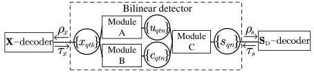
Refer to caption
Fig. 4: Top: an equivalent graph of Fig. 3 for the achievable rate analysis. Bottom: a graphical illustration of the SE between the bilinear detector and the 𝐗\mathbf{X}-decoder.

To facilitate the rate analysis, we combine modules A, B, and C, and all super variable nodes to form a bilinear detector of 𝐗\mathbf{X} and 𝐒D\mathbf{S}_{\rm D}, as illustrated in the upper plot of Fig. 4. Then we describe the state evolution between the bilinear detector and the two decoders as follows. At the 𝐗\mathbf{X}-decoder, the combination of two input AWGN observations with variances τr\tau_{r} and τo\tau_{o} can be considered as one AWGN observation with SNR ρx=1/τr+1/τo\rho_{x}=1/\tau_{r}+1/\tau_{o}. Furthermore, we assume that the decoder outputs {bxq​t​k}\{b_{x_{qtk}}\} can be characterized by a probability model with a single model parameter τx∈(0,τxmax)\tau_{x}\in(0,\tau_{x}^{\rm max}). τx→0\tau_{x}\to 0 represents that 𝐗\mathbf{X} is correctly detected and τx→τxmax\tau_{x}\to\tau_{x}^{\rm max} represents no information from the 𝐗\mathbf{X}-decoder, i.e., {xq​t​k}\{x_{qtk}\} are i.i.d. with xq​t​k∼1|𝒳|​∑xδ⁡(xq​t​k−x)x_{qtk}\sim\frac{1}{|\mathcal{X}|}\sum_{x}\delta(x_{qtk}-x). For example, considering BPSK modulation, bxq​t​kb_{x_{qtk}} is a log-likelihood ratio with model bxq​t​k=12​τx​xq​t​k+nxq​t​k,nxq​t​k∼𝒞​𝒩​(0,τx−1)b_{x_{qtk}}=\frac{1}{2\tau_{x}}x_{qtk}+n_{x_{qtk}},~n_{x_{qtk}}\sim\mathcal{CN}(0,\tau_{x}^{-1}) [32]. Through τx\tau_{x}, we establish a single-letter characterization of the 𝐗\mathbf{X}-decoder outputs. We then express the transfer function of the 𝐗\mathbf{X}-decoder as

τx=fx​(ρx).\displaystyle\tau_{x}=f_{x}(\rho_{x}). (50)

At the 𝐒D\mathbf{S}_{\rm D}-decoder, the inputs are the Rayleigh fading observations {dq​t​n}\{d_{qtn}\} in (46), where the Rayleigh model can be characterized by a single model parameter, i.e., SNR ρs=ζ​K/N−τpτp+τd\rho_{s}=\frac{\zeta K/N-\tau_{p}}{\tau_{p}+\tau_{d}}. Similarly to (50), we introduce state τs∈(0,τsmax)\tau_{s}\in(0,\tau_{s}^{\rm max}) for the establishment of the single-letter characterization of the 𝐒D\mathbf{S}_{\rm D}-decoder, and express the transfer function as

τs=fs​(ρs).\displaystyle\tau_{s}=f_{s}(\rho_{s}). (51)

At the bilinear detector, the output state is (ρx,ρs)(\rho_{x},\rho_{s}) and the input state is (τbs,τbs)(\tau_{{b}_{s}},\tau_{{b}_{s}}). The corresponding input-output relationship is expressed as

(ρx,ρs)=η⁡(τx,τs),\displaystyle(\rho_{x},\rho_{s})=\eta(\tau_{x},\tau_{s}), (52)

where η⁡(⋅)\eta(\cdot) can be determined by noting ρx=1τr+1τo\rho_{x}=\frac{1}{\tau_{r}}+\frac{1}{\tau_{o}} and ρs=ζ​K/N−τpτp+τd\rho_{s}=\frac{\zeta K/N-\tau_{p}}{\tau_{p}+\tau_{d}} with (τr,τo,τd,τp)(\tau_{r},\tau_{o},\tau_{d},\tau_{p}) given by the state equations and transfer functions involved in the bilinear detector, i.e., the iteration of (41), (44), (45), and (47)-(49) with vc=vu=K/N​ζ{v}_{c}={v}_{u}=K/N\zeta. Note that η⁡(⋅)\eta(\cdot) is determined by ratios N/MN/M, K/MK/M, and ζ=‖𝐆‖F2​‖𝐅‖F2N​‖𝐇‖F2\zeta=\frac{||\mathbf{G}||_{F}^{2}||\mathbf{F}||_{F}^{2}}{N||\mathbf{H}||_{F}^{2}}, noise variance σw2\sigma_{w}^{2}, and constraints 𝒳\mathcal{X} and 𝒮\mathcal{S}. fx​(⋅)f_{x}(\cdot) and fs​(⋅)f_{s}(\cdot) can be adjusted through different codebooks 𝒞x\mathcal{C}_{x} and 𝒞s\mathcal{C}_{s}. We can choose appropriate codebooks to ensure the SE convergence to τx=τs=0\tau_{x}=\tau_{s}=0, i.e., to achieve the error-free communication.

The lower plot of Fig. 4 gives an intuitive illustration of the condition for error-free communication. Specifically, it presents the SE between the detector and the 𝐗\mathbf{X}-decoder, where ηi​(⋅)\eta_{i}(\cdot) represents the ii-th entry of vector η⁡(⋅)\eta(\cdot) and fx−1​(⋅)f_{x}^{-1}(\cdot) is the inverse function of fx​(⋅)f_{x}(\cdot). Note that the SE between the detector and the 𝐒D\mathbf{S}_{\rm D}-decoder is similar and thus is omitted. The SE trajectory in the right plot of Fig. 4 describes how ρx\rho_{x} and (τx,τs)(\tau_{x},\tau_{s}) evolve according to (50)-(52). We see that when the decoder surface fx−1​(⋅)f_{x}^{-1}(\cdot) is below the detector surface η1​(⋅)\eta_{1}(\cdot), the SE trajectory ends at τx→0\tau_{x}\to 0 and τs→0\tau_{s}\to 0.

Theorem 2.

Consider the SE (50)-(52). Suppose fx​(ρx)f_{x}(\rho_{x}) and fs​(ρs)f_{s}(\rho_{s}) are monotonically decreasing functions with τxmax=fx​(0)\tau_{x}^{\rm max}=f_{x}(0) and τsmax=fs​(0)\tau_{s}^{\rm max}=f_{s}(0), respectively; further suppose ρx\rho_{x} and ρs\rho_{s} both monotonically decrease with respect to τx\tau_{x} or τs\tau_{s} in η⁡(τx,τs)\eta(\tau_{x},\tau_{s}). Then, the SE (50)-(52) converges. In particular, a sufficient and necessary condition for the SE convergence (τx,τs)→(0,0)(\tau_{x},\tau_{s})\to(0,0) is that there exists a 2-dimensional monotonic path ℒ\mathcal{L} starting from (τx,τs)=(τxmax,τsmax)(\tau_{x},\tau_{s})=(\tau_{x}^{\rm max},\tau_{s}^{\rm max}) and ending at (0,0)(0,0), such that (fx−1​(τx),fs−1​(τs))≺η⁡(τx,τs)(f_{x}^{-1}(\tau_{x}),f_{s}^{-1}(\tau_{s}))\prec\eta(\tau_{x},\tau_{s}) for any (τx,τs)∈ℒ(\tau_{x},\tau_{s})\in\mathcal{L}.

Proof.

Consider the following iterative steps of SE: (ρx0,ρs0)=η⁡(τx0,τs0)→τx1=fx​(ρx0),τs1=fs​(ρx1)→(ρx1,ρs1)=η⁡(τx1,τs1)→⋯(\rho_{x}^{0},\rho_{s}^{0})\!=\!\eta(\tau_{x}^{0},\tau_{s}^{0})\rightarrow\tau_{x}^{1}\!=\!f_{x}(\rho_{x}^{0}),\tau_{s}^{1}=f_{s}(\rho_{x}^{1})\rightarrow(\rho_{x}^{1},\rho_{s}^{1})\!=\!\eta(\tau_{x}^{1},\tau_{s}^{1})\rightarrow\cdots, where superscripts indicate iteration number and (τx0,τs0)=(τxmax,τsmax)(\tau_{x}^{0},\tau_{s}^{0})=(\tau_{x}^{\rm max},\tau_{s}^{\rm max}). In step 1, we have (0,0)≺(ρx0,ρs0)(0,0)\prec(\rho_{x}^{0},\rho_{s}^{0}) by noting ρx=1τr+1τo\rho_{x}=\frac{1}{\tau_{r}}+\frac{1}{\tau_{o}} and ρs=ζ​K/N−τpτp+τd\rho_{s}=\frac{\zeta K/N-\tau_{p}}{\tau_{p}+\tau_{d}} with (τr,τo,τd,τp)(\tau_{r},\tau_{o},\tau_{d},\tau_{p}) given by the iteration of (41), (44), (45), and (47)-(49). In step 2, given (0,0)≺(ρx0,ρs0)(0,0)\prec(\rho_{x}^{0},\rho_{s}^{0}) and the monotonicity of fx​(⋅)f_{x}(\cdot) and fs​(⋅)f_{s}(\cdot), we have (τx1,τs1)=(fx​(ρx0),fs​(ρs0))≺(fx​(0),fs​(0))=(τx0,τs0)(\tau_{x}^{1},\tau_{s}^{1})=(f_{x}(\rho_{x}^{0}),f_{s}(\rho_{s}^{0}))\prec(f_{x}(0),f_{s}(0))=(\tau_{x}^{0},\tau_{s}^{0}). In step 3, given (τx1,τs1)≺(τx0,τs0)(\tau_{x}^{1},\tau_{s}^{1})\prec(\tau_{x}^{0},\tau_{s}^{0}) and the monotonicity of η⁡(⋅)\eta(\cdot), we have (ρx0,ρs0)≺(ρx1,ρs1)(\rho_{x}^{0},\rho_{s}^{0})\prec(\rho_{x}^{1},\rho_{s}^{1}). We now prove (τx1,τs1)≺(τx0,τs0)(\tau_{x}^{1},\tau_{s}^{1})\prec(\tau_{x}^{0},\tau_{s}^{0}) and (ρx0,ρs0)≺(ρx1,ρs1)(\rho_{x}^{0},\rho_{s}^{0})\prec(\rho_{x}^{1},\rho_{s}^{1}). The subsequent processes are similar, and the SE converges to a fixed point (τx∗,τs∗,ρx∗,ρs∗)(\tau_{x}^{*},\tau_{s}^{*},\rho_{x}^{*},\rho_{s}^{*}) satisfying η⁡(τx∗,τs∗)=(ρx∗,ρs∗)=(fx−1​(τx∗),fs−1​(τs∗))\eta(\tau_{x}^{*},\tau_{s}^{*})=(\rho_{x}^{*},\rho_{s}^{*})=(f_{x}^{-1}(\tau_{x}^{*}),f_{s}^{-1}(\tau_{s}^{*})).

We first prove the necessity part. The SE convergence to (τx,τs)→(0,0)(\tau_{x},\tau_{s})\to(0,0) means that there is a corresponding SE trajectory starting from (τxmax,τsmax)(\tau_{x}^{\rm max},\tau_{s}^{\rm max}) and ending at (0,0)(0,0). Along the SE trajectory, the 𝐗\mathbf{X}-decoder surface and the 𝐒D\mathbf{S}_{\rm D}-decoder surface are both below the detector surface. Then, there exists one monotonic path ℒ\mathcal{L} which contains all points (τx,τs)(\tau_{x},\tau_{s}) on this SE trajectory, such that (fx−1​(τx),fs−1​(τs))≺η⁡(τx,τs)(f_{x}^{-1}(\tau_{x}),f_{s}^{-1}(\tau_{s}))\prec\eta(\tau_{x},\tau_{s}) for any (τx,τs)∈ℒ(\tau_{x},\tau_{s})\in\mathcal{L}.

We now prove the sufficiency part by contradiction. Suppose that the SE converges to a fixed point with (fx−1​(τx∗),fs−1​(τs∗))=η⁡(τx∗,τs∗)(f_{x}^{-1}(\tau_{x}^{*}),f_{s}^{-1}(\tau_{s}^{*}))=\eta(\tau_{x}^{*},\tau_{s}^{*}) and (0,0)≺(τx∗,τs∗)(0,0)\prec(\tau_{x}^{*},\tau_{s}^{*}). Given one monotonic path ℒ\mathcal{L} starting from (τxmax,τsmax)(\tau_{x}^{\rm max},\tau_{s}^{\rm max}) and ending at (0,0)(0,0), we select point (τ~x,τ~s)∈ℒ(\tilde{\tau}_{x},\tilde{\tau}_{s})\in\mathcal{L} which satisfies τ~s=τs∗\tilde{\tau}_{s}=\tau_{s}^{*}. We then obtain τx∗=τ~x\tau_{x}^{*}=\tilde{\tau}_{x}, τx∗<τ~x\tau_{x}^{*}<\tilde{\tau}_{x}, or τx∗>τ~x\tau_{x}^{*}>\tilde{\tau}_{x}. If τx∗=τ~x\tau_{x}^{*}=\tilde{\tau}_{x}, then (τx∗,τs∗)∈ℒ(\tau_{x}^{*},\tau_{s}^{*})\in\mathcal{L} and (fx−1​(τx∗),fs−1​(τs∗))≺η⁡(τx∗,τs∗)(f_{x}^{-1}(\tau_{x}^{*}),f_{s}^{-1}(\tau_{s}^{*}))\prec\eta(\tau_{x}^{*},\tau_{s}^{*}), which is in contradiction to the fixed point hypothesis; If τx∗<τ~x\tau_{x}^{*}<\tilde{\tau}_{x}, then f−1​(τs∗)=f−1​(τ~s)<η2​(τ~x,τ~s)<η2​(τx∗,τs∗)f^{-1}(\tau_{s}^{*})=f^{-1}(\tilde{\tau}_{s})<\eta_{2}(\tilde{\tau}_{x},\tilde{\tau}_{s})<\eta_{2}(\tau_{x}^{*},\tau_{s}^{*}), where the first inequality is from (τ~x,τ~s)∈ℒ(\tilde{\tau}_{x},\tilde{\tau}_{s})\in\mathcal{L} and the second inequality is from the monotonicity of η⁡(⋅)\eta(\cdot); If τx∗>τ~x\tau_{x}^{*}>\tilde{\tau}_{x}, we consider another point (τ¯x,τ¯s)∈ℒ(\bar{\tau}_{x},\bar{\tau}_{s})\in\mathcal{L} which satisfies τ¯x=τx∗\bar{\tau}_{x}=\tau_{x}^{*}. Given (fx−1​(τx∗),fs−1​(τs∗))=η⁡(τx∗,τs∗)(f_{x}^{-1}(\tau_{x}^{*}),f_{s}^{-1}(\tau_{s}^{*}))=\eta(\tau_{x}^{*},\tau_{s}^{*}) and the monotonicity of η⁡(⋅)\eta(\cdot), we have τ¯s<τs∗\bar{\tau}_{s}<\tau_{s}^{*}, since otherwise (fx−1​(τ¯x),fs−1​(τ¯s))<η⁡(τ¯x,τ¯s)(f_{x}^{-1}(\bar{\tau}_{x}),f_{s}^{-1}(\bar{\tau}_{s}))<\eta(\bar{\tau}_{x},\bar{\tau}_{s}) is not fulfilled. Then, two points (τ¯x,τ¯s)(\bar{\tau}_{x},\bar{\tau}_{s}) and (τ~x,τ~s)(\tilde{\tau}_{x},\tilde{\tau}_{s}) belongs to ℒ\mathcal{L} with τ¯x>τ~x\bar{\tau}_{x}>\tilde{\tau}_{x} and τ¯s<τ~s\bar{\tau}_{s}<\tilde{\tau}_{s}, which is in contradiction to the monotonic requirement of ℒ\mathcal{L}. ∎

Remark 2.

Generally speaking, fx​(ρx)f_{x}(\rho_{x}) (or fs​(ρs)f_{s}(\rho_{s})) is a monotonically decreasing function [34], which means that a higher SNR ρx\rho_{x} (or ρs\rho_{s}) leads to a lower estimation error represented by τx\tau_{x} (or τs\tau_{s}). The monotonicity of η⁡(τx,τs)\eta(\tau_{x},\tau_{s}) is from the similar fact. It is noteworthy that the number of possible 2-dimensional paths ℒ\mathcal{L} is infinite, and error-free communication requires only one path to satisfy the above-mentioned condition.

Definition 1.

We say that the transfer functions η⁡(⋅)\eta(\cdot), ψx​(⋅)\psi_{x}(\cdot), and ψs​(⋅)\psi_{s}(\cdot) satisfy the matching condition under ℒ\mathcal{L} if along a 22-dimensional monotonic path ℒ\mathcal{L} whose coordinates start from (τxmax,τsmax)(\tau_{x}^{\rm max},\tau_{s}^{\rm max}) and end at (0,0)(0,0), such that

(fx−1​(τx),fs−1​(τs))=η⁡(τx,τs).\displaystyle(f_{x}^{-1}(\tau_{x}),f_{s}^{-1}(\tau_{s}))=\eta(\tau_{x},\tau_{s}). (53)

The matching condition is the critical condition for error-free communication. In the matching condition under ℒ\mathcal{L}, all points in ℒ\mathcal{L} are fixed points; If (fx−1​(τx),fs−1​(τs))=η⁡(τx,τs)−(Δx,Δs)(f_{x}^{-1}(\tau_{x}),f_{s}^{-1}(\tau_{s}))\!=\!\eta(\tau_{x},\tau_{s})-(\Delta_{x},\Delta_{s}) with (0,0)≺(Δx,Δs)(0,0)\prec(\Delta_{x},\Delta_{s}), we achieve error-free communication; If (Δx,Δs)≺(0,0)(\Delta_{x},\Delta_{s})\prec(0,0), the SE stops at the initial point. For fx​(⋅)f_{x}(\cdot) and fs​(⋅)f_{s}(\cdot), the matching condition under ℒ\mathcal{L} gives the maxima of input SNRs ρx\rho_{x} and ρs\rho_{s} given outputs τx\tau_{x} and τs\tau_{s}, which corresponds to the worst cases of the decoder transfer functions.

We now establish the rate analysis. Denote by RTR_{T} and RRR_{R} the information rates at the Tx and the RIS, respectively. Similarly to (50), we express vxv_{x} in (45) as a function of SNR ρx\rho_{x}, denoted by vx=ψx​(ρx)v_{x}=\psi_{x}(\rho_{x}). Let vp​s{v}_{ps} be the normalized estimation MSE of ∑tpt​sq​n\sum_{t}p_{t}{s_{qn}}, i.e., vp​s{v}_{ps} can be expressed as vp​s=𝔼{dt},{pt},bs[∑t|pt|2ζ​K/N−τp{v}_{ps}=\mathbb{E}_{\{{d}_{t}\},\{{p}_{t}\},b_{s}}[\sum_{t}\frac{|{p}_{t}|^{2}}{\zeta K/N-\tau_{p}} var(s|{dt},{pt},s∼p(s|bs;τs);τp,τd)]\text{var}(s|\{{d}_{t}\},\{{p}_{t}\},s\sim p(s|b_{s};\tau_{s});\tau_{p},\tau_{d})]. Similarly to (51), we further express vp​sv_{ps} as vp​s=ψs​(ρs)v_{ps}=\psi_{s}(\rho_{s}). Let ψx,un​(ρx)\psi_{x,{\rm un}}(\rho_{x}) and ψs,un​(ρs)\psi_{s,{\rm un}}(\rho_{s}) be the special forms of ψx​(ρx)\psi_{x}(\rho_{x}) and ψs​(ρx)\psi_{s}(\rho_{x}) obtained for uncoded 𝐗\mathbf{X} and 𝐒D\mathbf{S}_{\rm D}. Note that ψx,un​(ρx)≥ψx​(ρx)\psi_{x,{\rm un}}(\rho_{x})\geq\psi_{x}(\rho_{x}) and ψs,un​(ρs)≥ψs​(ρs)\psi_{s,{\rm un}}(\rho_{s})\geq\psi_{s}(\rho_{s}) [35].

Theorem 3.

For the proposed SAPIT-MIMO transceiver with SE (50)-(52), the maximal achievable sum rate is

RT+RR\displaystyle R_{T}\!+\!R_{R} =∫0ρx0K​ψx,un​(ρx)​d​ρx+∫0ρs0N−NPT​ψs,un​(ρs)​d​ρs\displaystyle\!=\int_{0}^{\rho_{x}^{0}}\!K\psi_{x,{\rm un}}(\rho_{x})d\rho_{x}+\int_{0}^{\rho_{s}^{0}}\!\frac{N\!-\!N_{\rm P}}{T}\psi_{s,{\rm un}}(\rho_{s})d\rho_{s}
+supℒ∈𝒞∫ℒ(Kψx(η1(τx,τs)),N−NPTψs(η2(τx,τs)))\displaystyle\!+\!\sup_{\mathcal{L}\in\mathcal{C}}\int_{\mathcal{L}}\!\left(\!K\psi_{x}(\eta_{1}(\tau_{x},\tau_{s})),\frac{N\!-\!N_{\rm P}}{T}\psi_{s}(\eta_{2}(\tau_{x},\tau_{s}))\!\right)
⋅d​η​(τx,τs),\displaystyle\hskip 136.5733pt\boldsymbol{\cdot}d\eta(\tau_{x},\tau_{s}), (54)

where (ρx0,ρs0)=η⁡(τxmax,τsmax)(\rho_{x}^{0},\rho_{s}^{0})=\eta(\tau_{x}^{\rm max},\tau_{s}^{\rm max}); sup\sup denotes supremum operation and 𝒞\mathcal{C} is the set of all 22-dimensional monotonic paths starting from (τxmax,τsmax)(\tau_{x}^{\rm max},\tau_{s}^{\rm max}) and ending at (0,0)(0,0); ∫ℒ[K​ψx​(η1​(⋅)),N−NPT​ψs​(η2​(⋅))]⋅d​η​(⋅)\int_{\mathcal{L}}\left[K\psi_{x}(\eta_{1}(\cdot)),\frac{N-N_{\rm P}}{T}\psi_{s}(\eta_{2}(\cdot))\right]\boldsymbol{\cdot}d\eta(\cdot) is a line integral obtained by using the matching condition under ℒ\mathcal{L}.

Proof.

Recall that the detector outputs can be treated as the AWGN and Rayleigh-fading observations of xq​t​kx_{qtk} and sq​ns_{qn}. From [23], in the AWGN model of xq​t​kx_{qtk}, achievable RTR_{T} equals the area under curve K​ψx​(ρx)K\psi_{x}(\rho_{x}) from ρx=0\rho_{x}=0 to η1​(0,0)\eta_{1}(0,0), i.e., RT=K​∫0η1​(0,0)ψx​(ρx)​d​ρxR_{T}=K\int_{0}^{\eta_{1}(0,0)}\psi_{x}(\rho_{x})d\rho_{x}. We extend the above relationship between RTR_{T} and ψx​(ρx)\psi_{x}(\rho_{x}) to the Rayleigh fading model of sq​ns_{qn}. Specifically, by regarding pq​t​n​sq​n,t=1,…,Tp_{qtn}s_{qn},t=1,...,T as a single random vector, we have RR=N−NPT​∫0η2​(0,0)ψs​(ρs)​d​ρsR_{R}=\frac{N-N_{\rm P}}{T}\int_{0}^{\eta_{2}(0,0)}\psi_{s}(\rho_{s})d\rho_{s}. Then, we have RT+RR=K​∫0η1​(0,0)ψx​(ρx)​d​ρx+N−NPT​∫0η2​(0,0)ψs​(ρs)​d​ρsR_{T}+R_{R}=K\int_{0}^{\eta_{1}(0,0)}\psi_{x}(\rho_{x})d\rho_{x}+\frac{N-N_{\rm P}}{T}\int_{0}^{\eta_{2}(0,0)}\psi_{s}(\rho_{s})d\rho_{s}. We then divide each of the two integrals into two parts, i.e., the one from (0,0)(0,0) to η⁡(τxmax,τsmax)\eta(\tau_{x}^{\rm max},\tau_{s}^{\rm max}), and the other from η⁡(τxmax,τsmax)\eta(\tau_{x}^{\rm max},\tau_{s}^{\rm max}) to η⁡(0,0)\eta(0,0). In the first part, the maximum of K​∫0η1​(τxmax,τsmax)ψx​(ρx)​d​ρx+N−NPT​∫0η2​(τxmax,τsmax)ψs​(ρs)​d​ρsK\int_{0}^{\eta_{1}(\tau_{x}^{\rm max},\tau_{s}^{\rm max})}\psi_{x}(\rho_{x})d\rho_{x}+\frac{N-N_{\rm P}}{T}\int_{0}^{\eta_{2}(\tau_{x}^{\rm max},\tau_{s}^{\rm max})}\psi_{s}(\rho_{s})d\rho_{s} is obtained if ψx​(⋅)=ψx,un​(⋅)\psi_{x}(\cdot)=\psi_{x,{\rm un}}(\cdot) and ψs​(⋅)=ψs,un​(⋅)\psi_{s}(\cdot)=\psi_{s,{\rm un}}(\cdot). Correspondingly, the decoders’ transfer functions satisfy τxmax=fx​(ρx)\tau_{x}^{\rm max}=f_{x}(\rho_{x}) and τsmax=fs​(ρs)\tau_{s}^{\rm max}=f_{s}(\rho_{s}) from (ρx,ρs)=(0,0)(\rho_{x},\rho_{s})=(0,0) to η⁡(τxmax,τsmax)\eta(\tau_{x}^{\rm max},\tau_{s}^{\rm max}). In the second part, we consider the maximum of K​∫η1​(τxmax,τsmax)η1​(τx0,τs0)ψx​(ρx)​d​ρx+N−NPT​∫η2​(τxmax,τsmax)η2​(τx0,τs0)ψs​(ρs)​d​ρsK\int_{\eta_{1}(\tau_{x}^{\rm max},\tau_{s}^{\rm max})}^{\eta_{1}(\tau_{x}^{0},\tau_{s}^{0})}\psi_{x}(\rho_{x})d\rho_{x}+\frac{N-N_{\rm P}}{T}\int_{\eta_{2}(\tau_{x}^{\rm max},\tau_{s}^{\rm max})}^{\eta_{2}(\tau_{x}^{0},\tau_{s}^{0})}\psi_{s}(\rho_{s})d\rho_{s}. From the discussion below Definition 1, this maximum is obtained by using the matching condition and considering all possible paths ℒ\mathcal{L}, which concludes the proof. ∎

Remark 3.

Theorem 3 suggests that the matching condition is the necessary condition to achieve the maximum of RT+RRR_{T}+R_{R}. Although the choice of ℒ∈𝒞\mathcal{L}\in\mathcal{C} is infinite, we find from simulations that the differences of ∫ℒ[K​ψx​(η1​(⋅)),N−NPT​ψs​(η2​(⋅))]⋅d​η​(⋅)\int_{\mathcal{L}}\left[K\psi_{x}(\eta_{1}(\cdot)),\frac{N-N_{\rm P}}{T}\psi_{s}(\eta_{2}(\cdot))\right]\boldsymbol{\cdot}d\eta(\cdot) under different paths are small. In practice, we can randomly generate some paths belonging to the set 𝒞\mathcal{C} (e.g., a straight line from (τxmax,τsmax)(\tau_{x}^{\rm max},\tau_{s}^{\rm max}) to (0,0)(0,0)) and choose the one with maximal ∫ℒ[K​ψx​(η1​(⋅)),N−NPT​ψs​(η2​(⋅))]⋅d​η​(⋅)\int_{\mathcal{L}}\left[K\psi_{x}(\eta_{1}(\cdot)),\frac{N-N_{\rm P}}{T}\psi_{s}(\eta_{2}(\cdot))\right]\boldsymbol{\cdot}d\eta(\cdot). Along the selected path, the codes at the Tx and the Rx are then designed to fulfill (fx−1​(τx),fs−1​(τs))=η⁡(τx,τs)−(Δx,Δs)(f_{x}^{-1}(\tau_{x}),f_{s}^{-1}(\tau_{s}))=\eta(\tau_{x},\tau_{s})-(\Delta_{x},\Delta_{s}) with Δx\Delta_{x} and Δs\Delta_{s} taking small values. Recall that fx​(⋅)f_{x}(\cdot) and fs​(⋅)f_{s}(\cdot) are evaluated under the AWGN model and the Rayleigh fading model, respectively. We can borrow the tools developed in [33] and [35] for the design of curve-matching codes.

IV-D Some Extensions

We now apply the SE equations to some special cases with minor modifications. Specifically, if the direct link is blocked, i.e., 𝐇=𝟎\mathbf{H}=\mathbf{0}, we delete the computation of τr{\tau}_{r}, and modify τd=N/M​vu+σw2{\tau}_{d}=N/M{v}_{u}+\sigma_{w}^{2} in (41) and vx=𝔼o,bx​[var⁡(x|o,x∼p⁡(x|bx;τx);τo)]{v}_{x}=\mathbb{E}_{o,b_{x}}[{\rm var}(x|o,x\sim p(x|b_{x};\tau_{x});{\tau}_{o})] in (45). In an uncoded system, we set αq​n​(s)=1/|𝒮|\alpha_{qn}(s)=1/|\mathcal{S}| and βq​t​k​(x)=1/|𝒳|{\beta}_{qtk}(x)=1/|\mathcal{X}| for the computation of vxv_{x} in (45) and vsv_{s} in (47), respectively. For example, when BPSK modulation is adopted for xq​t​kx_{qtk}, (45) reduces to vx=1−∫−∞∞(πτr)−1/2tanh(2Re(R)/τr){v}_{x}=1-\int_{-\infty}^{\infty}(\pi{\tau}_{r})^{-1/2}\tanh(2{\rm Re}(R)/{\tau}_{r}) exp(−(Re(R)−1)2/τr)dRe(R){\rm exp}(-({\rm Re}(R)-1)^{2}/{\tau}_{r})d{\rm Re}(R) [36]. In a coded system with separate detection and decoding, we treat the system as uncoded in iterative detection, followed by conventional decoding operations. For the achievable rate calculation of the separate detection and decoding, we set ψx​(⋅)=ψx,un​(⋅)\psi_{x}(\cdot)=\psi_{x,{\rm un}}(\cdot) and ψs​(⋅)=ψs,un​(⋅)\psi_{s}(\cdot)=\psi_{s,{\rm un}}(\cdot). Then the fixed-point (ρx∗,ρs∗)(\rho_{x}^{*},\rho_{s}^{*}) can be obtained through the SE (50)-(52) until convergence, and (3) reduces to RT+RR≤K​∫0ρx∗ψx,un​(ρx)+N−NPT​∫0ρs∗ψs,un​(ρs)​d​ρsR_{T}+R_{R}\leq K\int_{0}^{\rho_{x}^{*}}\psi_{x,{\rm un}}(\rho_{x})+\frac{N-N_{\rm P}}{T}\int_{0}^{\rho_{s}^{*}}\psi_{s,{\rm un}}(\rho_{s})d\rho_{s}. Correspondingly, the decoder transfer functions for maximal achievable sum rate should fulfill fx​(ρx)=τxmaxf_{x}(\rho_{x})=\tau_{x}^{\rm max} and fs​(ρs)=τsmaxf_{s}(\rho_{s})=\tau_{s}^{\rm max} from (ρx,ρs)=(0,0)(\rho_{x},\rho_{s})=(0,0) to (ρx∗,ρs∗)(\rho_{x}^{*},\rho_{s}^{*}), and then sharply reduce to fx​(ρx∗)→0f_{x}(\rho_{x}^{*})\to 0 and fs​(ρs∗)→0f_{s}(\rho_{s}^{*})\to 0.

V Numerical Results

V-A Preliminaries

In this section, we evaluate the performance of Algorithm 1. Consider a three-dimensional (3D) Cartesian coordinate where Tx, Rx and RIS are respectively located at (0,0,1.5)(0,0,1.5), (0,500,11.5)(0,500,11.5) and (10,490,11.5)(10,490,11.5) in meters. The large-scale fading model is βloss=β0​(d3​D/d0)−α¯\beta_{\rm{loss}}=\beta_{0}(d_{\rm{3D}}/d_{0})^{-\bar{\alpha}}, where d0d_{0} denotes the reference distance, β0\beta_{0} denotes the fading at the reference distance, α¯\bar{\alpha} denotes the fading exponent, and d3​Dd_{\rm{3D}} denotes the distance. We set d0=1d_{0}=1 m, β0=−30\beta_{0}=-30 dB, α¯=2.2\bar{\alpha}=2.2 for the Tx-RIS and RIS-Rx links, and α¯=3.5\bar{\alpha}=3.5 for the Tx-Rx link [9]. Then the fading βlossTx→RIS\beta_{\rm{loss}}^{\rm{Tx}\to\rm{RIS}}, βlossRIS→Rx\beta_{\rm{loss}}^{\rm{RIS}\to\rm{Rx}} and βlossTx→Rx\beta_{\rm{loss}}^{\rm{Tx}\to\rm{Rx}} respectively for the Tx-RIS, RIS-Rx, and Tx-Rx links can be calculated according to the above fading model and the 3D coordinates. We adopt the Rayleigh fading model as the small-scale fading for all channels, i.e., gm​n∼𝒞​𝒩​(gm​n,0,βlossRIS→Rx)g_{mn}\sim\mathcal{CN}(g_{mn};0,\sqrt{\beta_{\rm{loss}}^{\rm{RIS}\to\rm{Rx}}}), fn​k∼𝒞​𝒩​(fn​k,0,βlossTx→RIS)f_{nk}\sim\mathcal{CN}(f_{nk};0,\sqrt{\beta_{\rm{loss}}^{\rm{Tx}\to\rm{RIS}}}), and hm​k∼𝒞​𝒩​(hm​k,0,βlossTx→Rx)h_{mk}\sim\mathcal{CN}(h_{mk};0,\sqrt{\beta_{\rm{loss}}^{\rm{Tx}\to\rm{Rx}}}) [4]. We consider that the noise power spectrum is −150-150 dBm/Hz and the system bandwidth is 11 MHz. Note that the RIS phase switching frequency of up to 11 MHz can be realized by the existing RIS prototypes [24]. Unless otherwise specified, we set N=512N=512, M=512M=512, K=64K=64, NP=40N_{\rm P}=40, Q=103Q=10^{3}, and T∈{1,2,4}T\in\{1,2,4\}. We consider the following baseline schemes in comparison:

  • •

    W/O RIS: No RIS is deployed, i.e., 𝐆=𝐅=𝟎\mathbf{G}=\mathbf{F}=\mathbf{0} and system model (1) reduces to 𝐲q​t=𝐇𝐱q​t+𝐰q​t\mathbf{y}_{qt}=\mathbf{H}\mathbf{x}_{qt}+\mathbf{w}_{qt}. We use Turbo-LMMSE algorithm [33] to detect 𝐱q​t\mathbf{x}_{qt}. Similarly to Algorithm 1, Turbo-LMMSE algorithm consists of a detector and a decoder with transfer functions ηturbo​(⋅)\eta_{\rm turbo}(\cdot) and ψturbo​(⋅)\psi_{\rm turbo}(\cdot), respectively. We calculate the achievable rate of the Tx under matching condition ηturbo−1​(⋅)=ψturbo​(⋅)\eta^{-1}_{\rm turbo}(\cdot)=\psi_{\rm turbo}(\cdot).

  • •

    Random phase: The phases of RIS elements are randomly chosen from the adjustable phase angles θi,i=1,…,|𝒮|\theta_{i},i=1,...,|\mathcal{S}|. Turbo-LMMSE is used based on system model 𝐲q​t=𝐁q​𝐱q​t+𝐰q​t\mathbf{y}_{qt}=\mathbf{B}_{q}\mathbf{x}_{qt}+\mathbf{w}_{qt} where 𝐁q=𝐆​diag​(𝐬q)​𝐅+𝐇\mathbf{B}_{q}=\mathbf{G}{\rm diag}(\mathbf{s}_{q})\mathbf{F}+\mathbf{H} is assumed to be known by the Rx.

  • •

    Passive beamforming: The algorithm in [4] is adopted to optimize the reflection phase, where the phase angles {θi}\{\theta_{i}\} are allowed to take values continuously in [0,2​π][0,2\pi]. Turbo-LMMSE is used at the Rx.

  • •

    SAPIT with TMP: Consider the proposed SAPIT technique with TMP algorithm [9] used at the Rx. The TMP algorithm is modified to exploit the Tx codebook 𝒞x\mathcal{C}_{x} and the RIS codebook 𝒞s\mathcal{C}_{s}.

V-B Performance Comparisons

Fig. 5 shows the MSE performance against the iteration number of Algorithm 1, where the MSE of 𝐗\mathbf{X} (or 𝐒D\mathbf{S}_{\rm D}) is normalized by the total number of elements of 𝐗\mathbf{X} (or 𝐒D\mathbf{S}_{\rm D}). BPSK and quadrature phase-shift keying (QPSK) are adopted at the RIS and the Tx, respectively. In the left plot of Fig. 5, we assume that the direct link is blocked, i.e., 𝐇=𝟎\mathbf{H}=\mathbf{0}, and that no channel encoding/decoding is used. We see that the SE results (dashed lines) coincide with the numerical simulations (solid lines), implying that the SE provides a good performance bound even for a system of moderate size. In the right plot of Fig. 5, rate-1/21/2 convolutional codes with generator polynomials (171,133)(171,133) are adopted at both the Tx and the RIS, and random interleaving is applied after channel encoding. The trend in the right plot of Fig. 5 is similar to that in the left plot of Fig. 5.

Fig. 5: MSE versus iteration number. Left: uncoded system with transmit power 1212 dBm in the absence of direct link. Right: coded system with transmit power 66 dBm in the presence of direct link.

Fig. 6 shows the BER performance versus transmit power, where the simulation settings in the left and right respectively follow those in the left and right of Fig. 5. The curve “Oracle bound (𝐗\mathbf{X})” means that 𝐒D\mathbf{S}_{\rm D} is known by the Rx when detecting 𝐗\mathbf{X}. The meaning of the curve “Oracle bound (𝐒D\mathbf{S}_{\rm D})” is analogous. For the passive beamforming scheme, 512512 quadrature amplitude modulation (QAM) is adopted at the Tx for almost the same information rates as that of SAPIT. In the left plot of Fig. 6, there is an evident gap between Algorithm 1 and TMP for the BER performances of 𝐗\mathbf{X} and 𝐒D\mathbf{S}_{\rm D}. Furthermore, Algorithm 1 approaches the lower bound as the Tx power increases. Passive beamforming has quite poor performance due to high-order modulation at the Tx, which confirms the superiority of SAPIT. In SAPIT, the estimates of RIS coefficients are treated as soft pilots for the estimates of the Tx signals, and vice versa. The trend in the right plot of Fig. 6 is similar. We now evaluate the impact of imperfect CSI. Specifically, we consider channel estimates 𝐆^\hat{\mathbf{G}}, 𝐅^\hat{\mathbf{F}}, and 𝐇^\hat{\mathbf{H}} with Gaussian errors Δ​𝐆=𝐆^−𝐆\Delta\mathbf{G}=\hat{\mathbf{G}}-\mathbf{G}, Δ​𝐅=𝐅^−𝐅\Delta\mathbf{F}=\hat{\mathbf{F}}-\mathbf{F}, and Δ​𝐇=𝐇^−𝐇\Delta\mathbf{H}=\hat{\mathbf{H}}-\mathbf{H}, respectively. The normalized MSE of the channel estimation is set −20-20 dB [27], and Algorithm 1 is modified to use the channel estimates. From the right plot of Fig. 6, we see that the imperfect CSI causes a slight performance loss. The reason is that it leads to the increase of the power of the equivalent noise. To see this, we rewrite (1) as 𝐲q​t=(𝐆^​diag​(𝐬q)​𝐅^+𝐇^)​𝐱q​t+𝐰^q​t\mathbf{y}_{qt}=\left(\hat{\mathbf{G}}\text{diag}(\mathbf{s}_{q})\hat{\mathbf{F}}+\hat{\mathbf{H}}\right)\mathbf{x}_{qt}+\hat{\mathbf{w}}_{qt} with equivalent noise 𝐰^q​t=𝐰q​t−(Δ​𝐇+𝐆^​diag​(𝐬q)​Δ​𝐅+Δ​𝐆​diag​(𝐬q)​𝐅)​𝐱q​t\hat{\mathbf{w}}_{qt}=\mathbf{w}_{qt}-(\Delta\mathbf{H}+\hat{\mathbf{G}}\text{diag}(\mathbf{s}_{q})\Delta\mathbf{F}+\Delta\mathbf{G}\text{diag}(\mathbf{s}_{q})\mathbf{F})\mathbf{x}_{qt}.

Fig. 6: BER versus transmit power. T=2T=2. Left: uncoded system in the absence of direct link. Right: coded system with direct link.

Fig. 7 shows the achievable sum-rate comparisons. For the SAPIT scheme, we calculate RT+RRR_{T}+R_{R} by the right-hand side of (3), where we randomly choose 1010 curves (τx,τs)(\tau_{x},\tau_{s}) with coordinates starting from (τxmax,τsmax)(\tau_{x}^{\rm max},\tau_{s}^{\rm max}) and ending at (0,0)(0,0). In the left plot of Fig. 7, 1616 QAM is adopted at the Tx and θ∈{0,π}\theta\in\{0,\pi\} is adopted at the RIS. As the RIS element number increases, all schemes (except no RIS) achieves a rate improvement. Furthermore, the SAPIT scheme achieves considerable superiority over the baselines and doubles the achievable sum rate of the passing beamforming scheme at N=800N=800. This superiority is also seen in the right plot of Fig. 7, where 6464 QAM and θ∈{0,π2,π,3​π2}\theta\in\{0,\frac{\pi}{2},\pi,\frac{3\pi}{2}\} are used at the Tx and the RIS, respectively. We note that the small rate gain by passive beamforming is due to the large sizes of the transceiver arrays, or more specifically, due to the fact that the beamforming gain by adjusting the RIS coefficients reduces as the number of spatial streams increases.

Fig. 7: Achievable sum rate versus the number of RIS elements with direct link and T=1T=1. Left: BPSK and 16QAM at the RIS and the Tx with transmit power 88 dBm. Right: QPSK and 64QAM at the RIS and the Tx with transmit power 1212 dBm.

VI Conclusions

In this paper, we proposed a novel SAPIT transceiver in the coded RIS-aided MIMO system. We established an auxiliary system model and developed a message-passing algorithm to solve the bilinear detection problem. We further developed the SE to predict the algorithm performance. Based on the SE, we analyzed the achievable sum rate of the Tx and the RIS. Finally, we conducted simulations to validate the SE analysis and show the superiority of the SAPIT scheme over the passive beamforming counterpart in achievable sum rate.

Appendix A

A-A Preliminaries

We first introduce a general recursion as a minor modification of [20, eq. (83)-(85)]. Consider an I×JI\times J random matrix 𝐀∈ℂI×J\mathbf{A}\in\mathbb{C}^{I\times J} with i.i.d. entries ai​j∼𝒞​𝒩​(ai​j,0,ζa/I)a_{ij}\sim\mathcal{CN}(a_{ij};0,\zeta_{a}/I). Define a set {𝜽in(l)∈ℂkn|n=1,…,nI.in=∑k=0n−1Ik+1,…,∑k=0nIk.l=0,…,L−1.}\{\boldsymbol{\theta}_{i_{n}}(l)\in\mathbb{C}^{k_{n}}|n=1,...,n_{I}.~i_{n}=\sum_{k=0}^{n-1}I_{k}+1,...,\sum_{k=0}^{n}I_{k}.~l=0,...,L-1.\} with I0=0I_{0}=0 and ∑n=1nIIn=I\sum_{n=1}^{n_{I}}I_{n}=I. Similarly, define a set {𝝋jn(l)∈ℂqn|n=1,…,nJ.jn=∑k=0n−1Jk+1,…,∑k=0nJk.l=0,…,L−1.}\{\boldsymbol{\varphi}_{j_{n}}(l)\in\mathbb{C}^{q_{n}}|n=1,...,n_{J}.~j_{n}=\sum_{k=0}^{n-1}J_{k}+1,...,\sum_{k=0}^{n}J_{k}.~l=0,...,L-1.\} with J0=0J_{0}=0 and ∑n=1nJJn=J\sum_{n=1}^{n_{J}}J_{n}=J. The recursion below involves the updates of 𝐪⁡(l),𝐦1​(l),𝐦2​(l)∈ℂJ\mathbf{q}(l),\mathbf{m}_{1}(l),\mathbf{m}_{2}(l)\in\mathbb{C}^{J} and 𝐞1​(l),𝐞2​(l),𝐯⁡(l)∈ℂI\mathbf{e}_{1}(l),\mathbf{e}_{2}(l),\mathbf{v}(l)\in\mathbb{C}^{I}. Specifically, given {𝜽in​(l)}\{\boldsymbol{\theta}_{i_{n}}(l)\} and {𝝋jn​(l)}\{\boldsymbol{\varphi}_{j_{n}}(l)\}, we have

𝐪⁡(l+1)=𝐀H​𝐯​(l)−(𝐦1​(l),𝐦2​(l))​𝝃​(l),\displaystyle\mathbf{q}(l+1)=\mathbf{A}^{H}\mathbf{v}(l)-\left(\mathbf{m}_{1}(l),\mathbf{m}_{2}(l)\right)\boldsymbol{\xi}(l),
vin​(l)=gl,n​(e1​in​(l),e2​in​(l),𝜽in​(l)),\displaystyle\hskip 1.0ptv_{i_{n}}(l)=g_{l,n}\left(e_{1i_{n}}(l),e_{2i_{n}}(l),\boldsymbol{\theta}_{i_{n}}(l)\right), (55a)
(𝐞1​(l),𝐞2​(l))=𝐀⁡(𝐦1​(l),𝐦2​(l))−𝐯⁡(l−1)​𝜸​(l)T,\displaystyle(\mathbf{e}_{1}(l),\mathbf{e}_{2}(l))\!=\!\mathbf{A}\left(\mathbf{m}_{1}(l),\mathbf{m}_{2}(l)\right)\!\!-\!\!\mathbf{v}(l-1)\boldsymbol{\gamma}(l)^{T},
(m1​jn​(l),m2​jn​(l))=fl,n​(qjn​(l),𝝋jn​(l)),\displaystyle\left(m_{1j_{n}}(l),m_{2j_{n}}(l)\right)\!=\!f_{l,n}\left(q_{j_{n}}(l),\boldsymbol{\varphi}_{j_{n}}(l)\right), (55b)

where 𝝃⁡(l)=(ζaI​∑n,in∂vin​(l)∂e1​in​(l),ζaI​∑i∂vin​(l)∂e2​in​(l))T∈ℝ2\boldsymbol{\xi}(l)=(\frac{\zeta_{a}}{I}\sum_{n,i_{n}}\frac{\partial v_{i_{n}}(l)}{\partial e_{1i_{n}}(l)},\frac{\zeta_{a}}{I}\sum_{i}\frac{\partial v_{i_{n}}(l)}{\partial e_{2i_{n}}(l)})^{T}\in\mathbb{R}^{2}, 𝜸⁡(l)=(ζaI​∑n,jn∂m1​jn​(l)∂qjn​(l),ζaI​∂m2​jn​(l)∂qjn​(l))T∈ℝ2\boldsymbol{\gamma}(l)=(\frac{\zeta_{a}}{I}\sum_{n,j_{n}}\frac{\partial m_{1j_{n}}(l)}{\partial q_{j_{n}}(l)},\frac{\zeta_{a}}{I}\frac{\partial m_{2j_{n}}(l)}{\partial q_{j_{n}}(l)})^{T}\in\mathbb{R}^{2}, and 𝐯⁡(−1)=𝟎\mathbf{v}(-1)=\mathbf{0}. (55) reduces to [20, eq. (83)-(85)] by letting nI=nJ=1n_{I}=n_{J}=1, and letting 𝜽in​(l)\boldsymbol{\theta}_{i_{n}}(l) and 𝝋jn​(l)\boldsymbol{\varphi}_{j_{n}}(l) invariant to recursion number ll. We note that in each iteration, both 𝐪⁡(l)\mathbf{q}(l) and (𝐞1​(l),𝐞2​(l))\mathbf{(}\mathbf{e}_{1}(l),\mathbf{e}_{2}(l)) are updated through a linear mixing of 𝐯⁡(l)\mathbf{v}(l) (or (𝐦1​(l),𝐦2​(l))\mathbf{(}\mathbf{m}_{1}(l),\mathbf{m}_{2}(l))) by random Gaussian matrix 𝐀\mathbf{A} (or 𝐀H\mathbf{A}^{H}) together with a point-wise subtraction. The linear mixing makes 𝐪⁡(l)\mathbf{q}(l) (or (𝐞1​(l),𝐞2​(l))\mathbf{(}\mathbf{e}_{1}(l),\mathbf{e}_{2}(l))) distributed as Gaussian vectors (or matrix) in the large system limit and the point-wise subtraction removes the correlation of the components of 𝐪⁡(l)\mathbf{q}(l) (or the rows of (𝐞1​(l),𝐞2​(l))\mathbf{(}\mathbf{e}_{1}(l),\mathbf{e}_{2}(l))). Furthermore, due to symmetry, the components of 𝐪⁡(l)\mathbf{q}(l) (or the rows of (𝐞1​(l),𝐞2​(l))\mathbf{(}\mathbf{e}_{1}(l),\mathbf{e}_{2}(l))) have the same distribution.

To formally describe the asymptotic properties of 𝐪⁡(l+1)\mathbf{q}(l+1) and (𝐞1​(l),𝐞2​(l))(\mathbf{e}_{1}(l),\mathbf{e}_{2}(l)), we introduce some definitions by following [22]. We say that a function ϕ⁡(⋅):ℂm→ℂ\phi(\cdot):\mathbb{C}^{m}\to\mathbb{C} is pseudo-Lipschitz of order 22, if there exists a constant c>0c>0 such that, for any 𝐱,𝐲∈ℂm\mathbf{x},\mathbf{y}\in\mathbb{C}^{m}: |ϕ⁡(𝐱)−ϕ⁡(𝐲)|≤c⁡(1+‖𝐱‖+‖𝐲‖)​‖𝐱−𝐲‖|\phi(\mathbf{x})-\phi(\mathbf{y})|\leq c\left(1+\|\mathbf{x}\|+\|\mathbf{y}\|\right)\|\mathbf{x}-\mathbf{y}\|. We say that the empirical distribution of vector sequences 𝐱i,i=1,…,N\mathbf{x}_{i},i=1,...,N (denoted by p^𝐱\hat{p}_{\mathbf{x}}) converges weakly to a probability density function p⁡(𝐱~)p(\tilde{\mathbf{x}}) if limN→∞𝔼p^𝐱​[ψ⁡(x)]=Ep𝐱~​[ψ⁡(x)]\lim_{N\to\infty}\mathbb{E}_{\hat{p}_{\mathbf{x}}}[\psi(x)]=E_{{p}_{\tilde{\mathbf{x}}}}[\psi(x)] for any bounded continuous function ψ⁡(⋅)\psi(\cdot). Our goal is to characterize the distribution of 𝐪⁡(l+1)\mathbf{q}(l+1) and (𝐞1​(l),𝐞2​(l))(\mathbf{e}_{1}(l),\mathbf{e}_{2}(l)) conditioned on the quantities previously calculated and used in (55). To this end, define 𝔖l1,l2\mathfrak{S}_{l_{1},l_{2}} as the probability space of {𝐪⁡(l)}l=0l1−1\{\mathbf{q}(l)\}_{l=0}^{l_{1}-1},{𝐯⁡(l)}l=0l1−1\{\mathbf{v}(l)\}_{l=0}^{l_{1}-1},{𝜽in​(l)}l=0l1−1\{\boldsymbol{\theta}_{i_{n}}(l)\}_{l=0}^{l_{1}-1}, {𝝋jn​(l)}l=1l2\{\boldsymbol{\varphi}_{j_{n}}(l)\}_{l=1}^{l_{2}}, {𝐞1​(l),𝐞2​(l)}l=1l2\{\mathbf{e}_{1}(l),\mathbf{e}_{2}(l)\}_{l=1}^{l_{2}}, and {𝐦1(l),\{\mathbf{m}_{1}(l), 𝐦2(l)}l=0l2\mathbf{m}_{2}(l)\}_{l=0}^{l_{2}}. Define matrix 𝐕l=[𝐯⁡(0),…,𝐯⁡(l−1)]\mathbf{V}_{l}=[\mathbf{v}(0),...,\mathbf{v}(l-1)] and 𝐌l=[𝐦1​(0),𝐦2​(0)​…,𝐦1​(l−1),𝐦2​(l−1)]\mathbf{M}_{l}=[\mathbf{m}_{1}(0),\mathbf{m}_{2}(0)...,\mathbf{m}_{1}(l-1),\mathbf{m}_{2}(l-1)]. Then we express 𝐯⁡(l)\mathbf{v}(l) as 𝐯⁡(l)=𝐯∥​(l)+𝐯⟂​(l)\mathbf{v}(l)=\mathbf{v}_{\parallel}(l)+\mathbf{v}_{\perp}(l), where 𝐯∥​(l)\mathbf{v}_{\parallel}(l) is the orthogonal projection of 𝐯⁡(l)\mathbf{v}(l) onto the column space of 𝐕l\mathbf{V}_{l}, and 𝐯⟂​(l)\mathbf{v}_{\perp}(l) is a vector in the orthogonal complementary space of the column space of 𝐕l\mathbf{V}_{l}. Furthermore, 𝐯∥​(l)\mathbf{v}_{\parallel}(l) can be expressed as 𝐯∥​(l)=∑i=1l−1αi​𝐯​(i)\mathbf{v}_{\parallel}(l)=\sum_{i=1}^{l-1}\alpha_{i}\mathbf{v}(i) with αi\alpha_{i} representing the ii-th projection coefficient. Analogously to the expression of 𝐯⁡(l)\mathbf{v}(l), let (𝐦1(l),𝐦2(l))=(𝐦1,∥(l),𝐦2,∥(l))+(𝐦1,⟂(l),𝐦2,⟂(l))(\mathbf{m}_{1}(l),\mathbf{m}_{2}(l))=(\mathbf{m}_{1,\parallel}(l),\mathbf{m}_{2,\parallel}(l))+(\mathbf{m}_{1,\perp}(l),\mathbf{m}_{2,\perp}(l)) where (𝐦1,∥(l),𝐦2,∥(l))=∑i=0l−1(𝐦1(i),𝐦2(i))𝜷i(\mathbf{m}_{1,\parallel}(l),\mathbf{m}_{2,\parallel}(l))=\sum_{i=0}^{l-1}(\mathbf{m}_{1}(i),\mathbf{m}_{2}(i))\boldsymbol{\beta}_{i} with 𝜷i∈ℝ2×2\boldsymbol{\beta}_{i}\in\mathbb{R}^{2\times 2}.

The state variables of the recursion (55) are τq​(l)∈ℝ\tau_{q}(l)\in\mathbb{R} and 𝚺⁡(l)∈ℂ2×2\boldsymbol{\Sigma}(l)\in\mathbb{C}^{2\times 2} given by

τq​(l)=ζa​∑n=1nIInI​𝔼​[|gl,n​(𝚺⁡(l)​𝐧,𝜽~n​(l))|2],\displaystyle\tau_{q}(l)=\zeta_{a}\sum_{n=1}^{n_{I}}\frac{I_{n}}{I}\mathbb{E}\left[\left|g_{l,n}\left(\sqrt{\boldsymbol{\Sigma}(l)}\mathbf{n},\tilde{\boldsymbol{\theta}}_{n}(l)\right)\right|^{2}\right], (56a)
𝚺(l)=ζa∑n=1nJJnI𝔼[fl,n(τq​(l)wq,𝝋~n(l))H×\displaystyle\boldsymbol{\Sigma}(l)=\zeta_{a}\sum_{n=1}^{n_{J}}\frac{J_{n}}{I}\mathbb{E}\Big[f_{l,n}(\sqrt{\tau_{q}(l)}w_{q},\tilde{\boldsymbol{\varphi}}_{n}(l))^{H}\times
fl,n(τq​(l)wq,𝝋~n(l))],\displaystyle\hskip 85.35826ptf_{l,n}(\sqrt{\tau_{q}(l)}w_{q},\tilde{\boldsymbol{\varphi}}_{n}(l))\Big], (56b)

where 𝐧∼𝒞​𝒩​(𝐧,0,𝐈)\mathbf{n}\sim\mathcal{CN}(\mathbf{n};0,\mathbf{I}), wq∼𝒞​𝒩​(wq,0,1)w_{q}\sim\mathcal{CN}(w_{q};0,1), and 𝚺⁡(0)=limJ→∞1J​(𝐦1​(0),𝐦2​(0))H​(𝐦1​(0),𝐦2​(0))\boldsymbol{\Sigma}(0)=\lim_{J\to\infty}\frac{1}{J}(\mathbf{m}_{1}(0),\mathbf{m}_{2}(0))^{H}(\mathbf{m}_{1}(0),\mathbf{m}_{2}(0)). The expectation 𝔼⁡[⋅]\mathbb{E}[\cdot] is taken over 𝐧\mathbf{n} and 𝜽~n​(l)\tilde{\boldsymbol{\theta}}_{n}(l) in (56a), and wqw_{q} and 𝝋~n​(l)\tilde{\boldsymbol{\varphi}}_{n}(l) in (56b).

Lemma 1.

Consider the recursion (55). Assume that the empirical distributions of 𝛉in​(l)\boldsymbol{\theta}_{i_{n}}(l), 𝛗jn​(l)\boldsymbol{\varphi}_{j_{n}}(l), and (m1​jn​(0),m2​jn​(0))T(m_{1j_{n}}(0),m_{2j_{n}}(0))^{T} respectively converge weakly to the probability distributions of random variables 𝛉~n​(l)\tilde{\boldsymbol{\theta}}_{n}(l), 𝛗~n​(l)\tilde{\boldsymbol{\varphi}}_{n}(l), and (m~1​n​(0)𝐶𝐿𝑂𝑆𝐸,(\tilde{m}_{1n}(0), 𝑂𝑃𝐸𝑁m~2​n​(0))T\tilde{m}_{2n}(0))^{T} with bounded second moments. Further, assume that the empirical second moments of those vectors respectively converge to the second moments of corresponding random variables. Assume that gl,n​(⋅)g_{l,n}(\cdot) and fl,n​(⋅)f_{l,n}(\cdot) are Lipschitz continuous and continuously differentiable almost everywhere with bounded derivatives. We have

𝐪⁡(l+1)|𝔖l+1,l\displaystyle\left.\mathbf{q}(l+1)\right|_{\mathfrak{S}_{l+1,l}}
=d∑i=0l−1αi​𝐪​(i+1)+𝐀~H​𝐯⟂​(l)+𝐌~l+1​𝐨l+1\displaystyle\quad\stackrel{{\scriptstyle\mathrm{d}}}{{=}}\sum_{i=0}^{l-1}\alpha_{i}\mathbf{q}(i+1)+\tilde{\mathbf{A}}^{H}\mathbf{v}_{\perp}(l)+\tilde{\mathbf{M}}_{l+1}\mathbf{o}_{l+1} (57a)
(𝐞1​(l),𝐞2​(l))|𝔖l,l,\displaystyle\left.(\mathbf{e}_{1}(l),\mathbf{e}_{2}(l))\right|_{\mathfrak{S}_{l,l}},
=d∑i=0l−1(𝐞1​(i),𝐞2​(i))​𝜷i+𝐀~​(𝐦1,⟂​(l),𝐦2,⟂​(l))+𝐕~l​(𝐨l,𝐨l),\displaystyle\quad\stackrel{{\scriptstyle\mathrm{d}}}{{=}}\sum_{i=0}^{l-1}(\mathbf{e}_{1}(i),\mathbf{e}_{2}(i))\boldsymbol{\beta}_{i}+\tilde{\mathbf{A}}(\mathbf{m}_{1,\perp}(l),\mathbf{m}_{2,\perp}(l))+\tilde{\mathbf{V}}_{l}(\mathbf{o}_{l},\mathbf{o}_{l}), (57b)

where 𝐀~\tilde{\mathbf{A}} is an independent copy of 𝐀\mathbf{A}; the columns of 𝐌~l\tilde{\mathbf{M}}_{l} (or 𝐕~l\tilde{\mathbf{V}}_{l}) form an orthogonal basis of the column space of 𝐌l\mathbf{M}_{l} (or 𝐕l\mathbf{V}_{l}) with 𝐌~lH​𝐌~l=N​𝐈l×l\tilde{\mathbf{M}}_{l}^{H}\tilde{\mathbf{M}}_{l}=N\mathbf{I}_{l\times l} (or 𝐕~lH​𝐕~l=J​𝐈l×l\tilde{\mathbf{V}}_{l}^{H}\tilde{\mathbf{V}}_{l}=J\mathbf{I}_{l\times l}; 𝐨l\mathbf{o}_{l}) is a vector of length ll whose elements converge to zero almost surely as I,J→∞I,J\to\infty. For any pseudo-Lipschitz functions ϕq​(⋅)\phi_{q}(\cdot) and ϕe​(⋅)\phi_{e}(\cdot) of order 2, we have

limJn→∞1Jn​∑jnϕq​(qjn​(l),𝝋jn​(l))\displaystyle\lim_{J_{n}\rightarrow\infty}\frac{1}{J_{n}}\sum_{j_{n}}\phi_{q}\left(q_{j_{n}}(l),\boldsymbol{\varphi}_{j_{n}}(l)\right)
= a.s. 𝔼[ϕq(τq​(l−1)wq,𝝋~n(l))],n=1,…,nJ,\displaystyle\quad\stackrel{{\scriptstyle\text{ a.s. }}}{{=}}\mathbb{E}\left[\phi_{q}\left(\sqrt{\tau_{q}(l-1)}w_{q},\tilde{\boldsymbol{\varphi}}_{n}(l)\right)\right],n=1,...,n_{J}, (58a)
limIn→∞1In​∑inϕe​(e1​in​(l),e2​in​(l),𝜽in​(l))\displaystyle\lim_{I_{n}\rightarrow\infty}\frac{1}{I_{n}}\sum_{i_{n}}\phi_{e}\left(e_{1i_{n}}(l),e_{2i_{n}}(l),\boldsymbol{\theta}_{i_{n}}(l)\right)
= a.s. 𝔼[ϕe(𝚺⁡(l)𝐧,𝜽~n(l))],n=1,…,nI,\displaystyle\quad\stackrel{{\scriptstyle\text{ a.s. }}}{{=}}\mathbb{E}\left[\phi_{e}\left(\sqrt{\boldsymbol{\Sigma}(l)}\mathbf{n},\tilde{\boldsymbol{\theta}}_{n}(l)\right)\right],n=1,...,n_{I}, (58b)

where wq∼𝒞​𝒩​(wq,0,1)w_{q}\sim\mathcal{CN}(w_{q};0,1) is independent of 𝛗~n​(l)\tilde{\boldsymbol{\varphi}}_{n}(l) and 𝐧∼𝒞​𝒩​(𝐧,0,𝐈)\mathbf{n}\sim\mathcal{CN}(\mathbf{n};0,\mathbf{I}) is independent of 𝛉~n​(l)\tilde{\boldsymbol{\theta}}_{n}(l); a= a.s. ba\stackrel{{\scriptstyle\text{ a.s. }}}{{=}}b represent aa equals bb almost surely.

Equations (57a) and (58a) in Lemma 1 mean that in the asymptotic regime I,J→∞I,J\to\infty, 𝐪⁡(l)\mathbf{q}(l) can be treated as a random Gaussian vector with i.i.d. entries of variance τq​(l)\tau_{q}(l); (57b) and (58b) mean that (𝐞1​(l),𝐞2​(l))(\mathbf{e}_{1}(l),\mathbf{e}_{2}(l)) can be treated as a random Gaussian matrix consisting of i.i.d. row vectors with covariance matrix 𝚺⁡(l)\boldsymbol{\Sigma}(l). The recursion (55) is a straightforward extension of [20, eq. (83)-(85)], where the difference is only the choice of nIn_{I}, nJn_{J}, 𝜽in​(l)\boldsymbol{\theta}_{i_{n}}(l), and 𝝋jn​(l)\boldsymbol{\varphi}_{j_{n}}(l). Correspondingly, Lemma 1 is an extension of [20, Lemma 3]. The proof of Lemma 1 is straightforward by borrowing the methodology in [20]. We note that the key to ensuring Lemma 1 is the point-wise subtraction in the left hand-side of (55) for decorrelation and the Gaussian rotational invariance provided by the random Gaussian matrix 𝐀\mathbf{A}.

A-B Proof

The results of Theorem 1 comprise parts 1) and 2) for the models of xq​t​kx_{qtk} and uq​t​nu_{qtn} at Module A, parts 3) and 4) for the models of xq​t​kx_{qtk} and cq​t​nc_{qtn} at Module B, and the SE equations including (41) at Module A, (44) at module B, and (45) and (47)-(49) at super variable nodes. Note that (45) and (47)-(49) at super variable nodes are obtained by using the SE equations at Modules A and B. Thus, it suffices to prove parts 1) and 2), and (41) at module A, and parts 3) and 4), and (44) at module B. We prove by showing that the message passing related to modules A and B are both special cases of recursion (55), as detailed below.

A-B1 State evolution related to module A

The message passing related to module A involves the estimates of xq​t​kx_{qtk} and uq​t​ku_{qtk}. Under the i.i.d. assumptions (in Assumption 1 of Theorem 1) on the decoder outputs {bxq​t​k}\{b_{x_{qtk}}\} (or {bsq​n}\{b_{s_{qn}}\}), the estimation processes of xq​t​kx_{qtk} and uq​t​ku_{qtk} are independent and identical at different sub-blocks qq and time-slot tt. In what follows, we focus on the message passing related to module A at one time-slot in a sub-block.

Specifically, for recursion matrix, let 𝐀=[𝐆,𝐇]\mathbf{A}=[\mathbf{G},\mathbf{H}] and ζa=1\zeta_{a}=1; for recursion vectors, let 𝐦2​(l)=𝟎\mathbf{m}_{2}(l)=\mathbf{0} and 𝐞2​(l)=𝟎\mathbf{e}_{2}(l)=\mathbf{0}; for recursion parameters, let nI=1n_{I}=1, I1=MI_{1}=M, and θi1=wi1\theta_{i_{1}}=w_{i_{1}} in (1), and let nJ=3n_{J}=3, (J1,J2,J3)=(NP,N−NP,K)(J_{1},J_{2},J_{3})=(N_{\rm P},N-N_{\rm P},K), 𝝋j1=(uj1,cj1,pj1)\boldsymbol{\varphi}_{j_{1}}=(u_{j_{1}},c_{j_{1}},p_{j_{1}}), 𝝋j2=(uj2,cj2,pj2,sj​2)\boldsymbol{\varphi}_{j_{2}}=(u_{j_{2}},c_{j_{2}},p_{j_{2}},s_{j2}), and 𝝋j3=(xj3,oj3)\boldsymbol{\varphi}_{j_{3}}=(x_{j_{3}},o_{j_{3}}). Then the correspondence between (55) and the message passing related to module A is given by

𝐪=(𝐮T,𝐱T)T−(𝐝T,𝐫T)T​and​𝐞1=𝐰−(𝐲−𝐛),\displaystyle\mathbf{q}=(\mathbf{u}^{T},\mathbf{x}^{T})^{T}-(\mathbf{d}^{T},\mathbf{r}^{T})^{T}~{\rm and}~\mathbf{e}_{1}=\mathbf{w}-(\mathbf{y}-\mathbf{b}), (59a)
vi1=g1​(ei1,wi1)=ei1−wi1,\displaystyle v_{i_{1}}=g_{1}(e_{i_{1}},w_{i_{1}})=e_{i_{1}}-w_{i_{1}}, (59b)
m1​j1=𝔼⁡(uj1|uj1−qj1,pj1;τd,τp)−uj1,\displaystyle m_{1j_{1}}=\mathbb{E}(u_{j_{1}}|u_{j_{1}}-q_{j_{1}},p_{j_{1}};{\tau}_{d},{\tau}_{p})-u_{j_{1}}, (59c)
m1​j2=𝔼[uj2|uj2−qj2,pj2,sj2∼πj2;τd,τp]−uj2,\displaystyle m_{1j_{2}}=\mathbb{E}[u_{j_{2}}|u_{j_{2}}-q_{j_{2}},p_{j_{2}},s_{j_{2}}\sim{\pi}_{j_{2}};{\tau}_{d},{\tau}_{p}]-u_{j_{2}}, (59d)
m1​j3=𝔼[xj3|xj3−qj3,oj3,xj3∼βj​3;τr,τo]−xj3,\displaystyle m_{1j_{3}}=\mathbb{E}[x_{j_{3}}|x_{j_{3}}-q_{j_{3}},o_{j_{3}},x_{j_{3}}\sim\beta_{j3};{\tau}_{r},{\tau}_{o}]-x_{j_{3}}, (59e)

with ξ1=1\xi_{1}=1 and γ1=−(KM​∑j=1Kvxjτr1+NM​∑j=1Nvujτd)=−τb(τbp+σw2)\gamma_{1}=-\left(\frac{K}{M}\sum_{j=1}^{K}\frac{v_{x_{j}}}{{\tau}_{r_{1}}}+\frac{N}{M}\sum_{j=1}^{N}\frac{v_{u_{j}}}{{\tau}_{d}}\right)=-\frac{{\tau}_{b}}{({\tau}_{b}^{\rm p}+\sigma_{w}^{2})}. Note that 𝔼(⋅|⋅)\mathbb{E}(\cdot|\cdot) in (59c)-(59e) are treated as functions, e.g., 𝔼(xj​3|⋅)\mathbb{E}(x_{j3}|\cdot) in (59e) are functions of qj​3q_{j3} and oj​3o_{j3}. These functions are Lipschitz continuous since the partial derivatives of these functions exist and are bounded everywhere. The corresponding functions var(⋅|⋅){\rm var}(\cdot|\cdot) are pseudo-Lipschitz of order 22. For example, considering (59e), we have var(xj​3|⋅)=∫|xj​3−𝔼(xj​3|⋅)|2p(xj​3|⋅)dxj​3{\rm var}(x_{j3}|\cdot)=\int|x_{j3}-\mathbb{E}(x_{j3}|\cdot)|^{2}p(x_{j3}|\cdot)dx_{j3}. Since 𝔼(xj​3|⋅)\mathbb{E}(x_{j3}|\cdot) is Lipschitz continuous and function |⋅|2|\cdot|^{2} is pseudo-Lipschitz of order 2, var(xj​3|⋅){\rm var}(x_{j3}|\cdot) belongs to pseudo-Lipschitz functions of order 2.

Applying (57a) in Lemma 1 for qj3=xj3−r1​j3q_{j_{3}}=x_{j_{3}}-r_{1j_{3}} in (59a), we prove part 1) of Theorem 1. Similarly, applying (57a) in Lemma 1 for qj2=uj2−dj2q_{j_{2}}=u_{j_{2}}-d_{j_{2}}, we prove part 2) of Theorem 1. Using (56b), we obtain Σ1,1=NPM​𝔼​[var⁡(uj1|dj1,pj1;τd,τp)]+N−NPM​𝔼​[var⁡(uj2|dj2,pj2,sj2∼πj2;τd,τp)]+KM​𝔼​[var⁡(xj​3|rj3,oj3,xj3∼βj​3;τr,τo)]=NM​vu+KM​vx\Sigma_{1,1}=\frac{N_{\rm P}}{M}\mathbb{E}[{\rm var}(u_{j_{1}}|d_{j_{1}},p_{j_{1}};{\tau}_{d},{\tau}_{p})]+\frac{N-N_{\rm P}}{M}\mathbb{E}[{\rm var}(u_{j_{2}}|d_{j_{2}},p_{j_{2}},s_{j_{2}}\sim{\pi}_{j_{2}};{\tau}_{d},{\tau}_{p})]+\frac{K}{M}\mathbb{E}[{\rm var}(x_{j3}|r_{j_{3}},o_{j_{3}},x_{j_{3}}\sim\beta_{j3};{\tau}_{r},\tau_{o})]=\frac{N}{M}{v}_{u}+\frac{K}{M}{v}_{x}. With Σ1,1=NM​vu+KM​vx\Sigma_{1,1}=\frac{N}{M}{v}_{u}+\frac{K}{M}{v}_{x} and (56a), we obtain τq=𝔼​|Σ1,1​n−wi|2=NM​vu+KM​vx+σw2=τr=τd\tau_{q}=\mathbb{E}|\sqrt{\Sigma_{1,1}}n-w_{i}|^{2}=\frac{N}{M}{v}_{u}+\frac{K}{M}{v}_{x}+\sigma_{w}^{2}=\tau_{r}=\tau_{d} in (41).

A-B2 State evolution related to module B

Similarly to the proof in the previous subsection, let 𝐀=𝐅\mathbf{A}=\mathbf{F}, and ζa=ζ\zeta_{a}=\zeta; nI=2n_{I}=2, (I1,I2)=(N−NP,NP)(I_{1},I_{2})=(N-N_{\rm P},N_{\rm P}), 𝜽i1=(di1−ui1,si1)=(wdi1,si1){\boldsymbol{\theta}}_{i_{1}}=(d_{i_{1}}-u_{i_{1}},s_{i_{1}})=(w_{d_{i_{1}}},s_{i_{1}}), and θi2=di2−ui2=wdi2{\theta}_{i_{2}}=d_{i_{2}}-u_{i_{2}}=w_{d_{i_{2}}}; nJ=1n_{J}=1, J1=KJ_{1}=K, and 𝝋j1=(xj1,r1​j1,αj1)\boldsymbol{\varphi}_{j_{1}}=(x_{j_{1}},r_{1j_{1}},{\alpha}_{j_{1}}). Then the correspondence between (55) and the message passing related to module B is given by

𝐪=𝐨−𝐱,𝐞1=𝐜,and​𝐞2=𝐩,\displaystyle\mathbf{q}=\mathbf{o}-\mathbf{x},~\mathbf{e}_{1}=\mathbf{c},~{\rm and}~\mathbf{e}_{2}=\mathbf{p}, (60a)
vi1=τoτp(𝔼[ci1|si1e1​i1+wdi1,e2​i1,si1∼πi1;τd,τp]−e2​i1),\displaystyle v_{i_{1}}=\frac{{\tau}_{o}}{{\tau}_{p}}\left(\mathbb{E}[c_{i_{1}}|s_{i_{1}}e_{1i_{1}}+w_{d_{i_{1}}},e_{2i_{1}},s_{i_{1}}\sim{\pi}_{i_{1}};{\tau}_{d},{\tau}_{p}]-e_{2i_{1}}\right), (60b)
vi2=τoτp(𝔼[ci2|e1​i2+wdi2,e2​i2;τd,τp]−e2​i2),\displaystyle v_{i_{2}}=\frac{{\tau}_{o}}{{\tau}_{p}}\left(\mathbb{E}[c_{i_{2}}|e_{1i_{2}}+w_{d_{i_{2}}},e_{2i_{2}};{\tau}_{d},{\tau}_{p}]-e_{2i_{2}}\right), (60c)
(m1​j1,m2​j1)=(xj,𝔼[xj1|rj1,xj1+qj1,xj1∼αj1;τr,τo]),\displaystyle(m_{1j_{1}},m_{2j_{1}})=\left(x_{j},\mathbb{E}[x_{j_{1}}|r_{j_{1}},x_{j_{1}}+q_{j_{1}},x_{j_{1}}\sim{\alpha}_{j_{1}};{\tau}_{r},{\tau}_{o}]\right), (60d)

with ξ2=ζ​τoτp​(1N​∑i=1Nvci−τpτp)=−1\xi_{2}=\frac{\zeta{\tau}_{o}}{{\tau}_{p}}(\frac{1}{N}\sum_{i=1}^{N}\frac{v_{c_{i}}-{\tau}_{p}}{{\tau}_{p}})=-1, ξ1=1\xi_{1}=1, γ2=ζN​∑j=1Kvxjτo=τpτo\gamma_{2}=\frac{\zeta}{N}\sum_{j=1}^{K}\frac{v_{x_{j}}}{{\tau}_{o}}=\frac{{\tau}_{p}}{{\tau}_{o}}, and γ1=0\gamma_{1}=0.

Applying (57a) with qj1=oj1−xj1q_{j_{1}}=o_{j_{1}}-x_{j_{1}}, we prove part 3) of Theorem 1. Applying (57b) with (e1​i,e2​i)=(−ci,pi)(e_{1i},e_{2i})=(-c_{i},p_{i}), we prove part 4) of Theorem 1. Using (56b), we obtain 𝚺=ζ​𝔼​[f1​(τo​wq,𝝋~1)H​f1​(τo​wq,𝝋~1)]=[ζ​KN,ζ​KN−ζ​KN​vx;ζ​KN−ζ​KN​vx,ζ​KN​vx]\boldsymbol{\Sigma}=\zeta\mathbb{E}[f_{1}(\sqrt{\tau_{o}}w_{q},\tilde{\boldsymbol{\varphi}}_{1})^{H}f_{1}(\sqrt{\tau_{o}}w_{q},\tilde{\boldsymbol{\varphi}}_{1})]=[\zeta\frac{K}{N},\zeta\frac{K}{N}-\zeta\frac{K}{N}{v}_{x};\zeta\frac{K}{N}-\zeta\frac{K}{N}{v}_{x},\zeta\frac{K}{N}{v}_{x}], which yields p⁡(ci|pi)=𝒞​𝒩​(ci,pi,ζ​KN​vx)p(c_{i}|p_{i})=\mathcal{CN}(c_{i};p_{i},\zeta\frac{K}{N}{v}_{x}) and pi∼𝒞​𝒩​(pi,0,ζ​KN−ζ​KN​vx)p_{i}\sim\mathcal{CN}(p_{i};0,\zeta\frac{K}{N}-\zeta\frac{K}{N}{v}_{x}). Then we obtain the AWGN model ci=pi+wcic_{i}=p_{i}+w_{c_{i}} in (43) with τp=ζ​KN​vx{\tau}_{p}=\zeta\frac{K}{N}{v}_{x} in (44). Using (56a) and [20, eq. (76)], we obtain τq=ζ𝔼[|g1(ci,pi,𝜽~i)|2]=ζτo2𝔼[∂∂pi(1τp(NPN𝔼[ci|di,pi;τd,τp]+N−NPN𝔼[ci|di,pi,si∼πi;τd,τp]−pi))]=τp2/(ζ(τp−vc))=τo\tau_{q}=\zeta\mathbb{E}\left[|g_{1}(c_{i},p_{i},\tilde{\boldsymbol{\theta}}_{i})|^{2}\right]=\zeta{\tau}_{o}^{2}\mathbb{E}[\frac{\partial}{\partial p_{i}}(\frac{1}{\tau_{p}}(\frac{N_{\rm P}}{N}\mathbb{E}[c_{i}|d_{i},p_{i};{\tau}_{d},{\tau}_{p}]+\frac{N-N_{\rm P}}{N}\mathbb{E}[c_{i}|d_{i},p_{i},s_{i}\sim{\pi}_{i};{\tau}_{d},{\tau}_{p}]-p_{i}))]={{\tau}_{p}^{2}/}{(\zeta({\tau}_{p}-{v}_{c}))}=\tau_{o} in (44), which concludes the proof.

References

  • [1] X. Yuan, Y.-J. A. Zhang, Y. Shi, W. Yan, and H. Liu, “Reconfigurable-intelligent-surface empowered wireless communications: Challenges and opportunities,” IEEE Wireless Commun., vol. 28, no. 2, pp. 136–143, Feb. 2021.
  • [2] Y. Liu, X. Liu, X. Mu, T. Hou, J. Xu, M. Di Renzo, and N. Al-Dhahir, “Reconfigurable intelligent surfaces: Principles and opportunities,” IEEE Communi. Surveys & Tutor., vol. 23, no. 3, pp. 1546–1577, May 2021.
  • [3] B. Zheng, C. You, W. Mei, and R. Zhang, “A survey on channel estimation and practical passive beamforming design for intelligent reflecting surface aided wireless communications,” IEEE Commun. Surveys & Tutor., vol. 24, no. 2, Feb 2022.
  • [4] S. Zhang and R. Zhang, “Capacity characterization for intelligent reflecting surface aided MIMO communication,” IEEE J. Sel. Areas Commun., vol. 38, no. 8, pp. 1823–1838, June 2020.
  • [5] T. Hou, Y. Liu, Z. Song, X. Sun, and Y. Chen, “MIMO-NOMA networks relying on reconfigurable intelligent surface: A signal cancellation-based design,” IEEE Transactions on Communications, vol. 68, no. 11, pp. 6932–6944, Aug. 2020.
  • [6] N. S. Perović, L.-N. Tran, M. Di Renzo, and M. F. Flanagan, “Achievable rate optimization for mimo systems with reconfigurable intelligent surfaces,” IEEE Trans. Wireless Commun., vol. 20, no. 6, pp. 3865–3882, Feb 2021.
  • [7] M. Di Renzo, A. Zappone, M. Debbah, M.-S. Alouini, C. Yuen, J. de Rosny, and S. Tretyakov, “Smart radio environments empowered by reconfigurable intelligent surfaces: How it works, state of research, and the road ahead,” IEEE J. Sel. Areas Commun., vol. 38, no. 11, pp. 2450–2525, July 2020.
  • [8] W. Yan, X. Yuan, and X. Kuai, “Passive beamforming and information transfer via large intelligent surface,” IEEE Wireless Commun. Lett., vol. 9, no. 4, pp. 533–537, Dec 2019.
  • [9] W. Yan, X. Yuan, Z.-Q. He, and X. Kuai, “Passive beamforming and information transfer design for reconfigurable intelligent surfaces aided multiuser MIMO systems,” IEEE J. Sel. Areas Commun., vol. 38, no. 8, June 2020.
  • [10] E. Basar, “Reconfigurable intelligent surface-based index modulation: A new beyond MIMO paradigm for 6G,” IEEE Trans. Wireless Commun., vol. 68, no. 5, pp. 3187–3196, Feb 2020.
  • [11] J. Yuan, M. Wen, Q. Li, E. Basar, G. C. Alexandropoulos, and G. Chen, “Receive quadrature reflecting modulation for RIS-empowered wireless communications,” IEEE Trans. Veh. Technol., vol. 70, no. 5, pp. 5121–5125, Apr. 2021.
  • [12] L. Zhang, X. Lei, Y. Xiao, and T. Ma, “Large intelligent surface-based generalized index modulation,” IEEE Commun. Lett., vol. 25, no. 12, pp. 3965–3969, Oct 2021.
  • [13] S. Lin, B. Zheng, G. C. Alexandropoulos, M. Wen, M. D. Renzo, and F. Chen, “Reconfigurable intelligent surfaces with reflection pattern modulation: Beamforming design and performance analysis,” IEEE Trans. Wireless Commun., vol. 20, no. 2, pp. 741–754, Dec. 2021.
  • [14] S. Lin, F. Chen, M. Wen, Y. Feng, and M. Di Renzo, “Reconfigurable intelligent surface-aided quadrature reflection modulation for simultaneous passive beamforming and information transfer,” IEEE Trans. Wireless Commun., vol. 21, no. 3, pp. 1469–1481, Aug. 2022.
  • [15] S. Guo, S. Lv, H. Zhang, J. Ye, and P. Zhang, “Reflecting modulation,” IEEE J. Sel. Areas Commun., vol. 38, no. 11, pp. 2548–2561, July 2020.
  • [16] H. Zhao, Y. Shuang, M. Wei, T. J. Cui, P. d. Hougne, and L. Li, “Metasurface-assisted massive backscatter wireless communication with commodity Wi-Fi signals,” Nat. commun., vol. 11, no. 1, p. 3926, Aug. 2020.
  • [17] R. Karasik, O. Simeone, M. D. Renzo, and S. Shamai Shitz, “Adaptive coding and channel shaping through reconfigurable intelligent surfaces: An information-theoretic analysis,” IEEE Trans. Commun., vol. 69, no. 11, pp. 7320–7334, July 2021.
  • [18] H. V. Cheng and W. Yu, “Degree-of-freedom of modulating information in the phases of reconfigurable intelligent surface,” arXiv preprint arXiv:2112.13787, 2021.
  • [19] D. L. Donoho, A. Maleki, and A. Montanari, “Message-passing algorithms for compressed sensing,” Proc. Nat. Acad. Sci. USA, vol. 106, no. 45, pp. 18 914–18 919, Nov. 2009.
  • [20] S. Rangan, “Generalized approximate message passing for estimation with random linear mixing,” arXiv preprint arXiv:1010.5141v2, Aug. 2012.
  • [21] J. T. Parker, P. Schniter, and V. Cevher, “Bilinear generalized approximate message passing—part i: Derivation,” IEEE Trans. Signal Process., vol. 62, no. 22, pp. 5839–5853, Sep. 2014.
  • [22] M. Bayati and A. Montanari, “The dynamics of message passing on dense graphs, with applications to compressed sensing,” IEEE Trans. Inf. Theory, vol. 57, no. 2, pp. 764–785, Feb. 2011.
  • [23] D. Guo, S. Shamai, and S. Verdu, “Mutual information and minimum mean-square error in Gaussian channels,” IEEE Trans. Inf. Theory, vol. 51, no. 4, pp. 1261–1282, Apr. 2005.
  • [24] L. Zhang, X. Q. Chen, S. Liu, Q. Zhang, J. Zhao, J. Y. Dai, G. D. Bai, X. Wan, Q. Cheng, G. Castaldi et al., “Space-time-coding digital metasurfaces,” Nat. commun., vol. 9, no. 1, pp. 1–11, Oct. 2018.
  • [25] R. Faqiri, C. Saigre-Tardif, G. C. Alexandropoulos, N. Shlezinger, M. F. Imani, and P. del Hougne, “Physfad: Physics-based end-to-end channel modeling of RIS-parametrized environments with adjustable fading,” IEEE Trans. Wireless Commun., vol. 22, no. 1, pp. 580–595, Aug. 2022.
  • [26] A. Rabault, L. L. Magoarou, J. Sol, G. C. Alexandropoulos, N. Shlezinger, H. V. Poor, and P. del Hougne, “On the tacit linearity assumption in common cascaded models of RIS-parametrized wireless channels,” arXiv preprint arXiv:2302.04993, 2023.
  • [27] Z.-Q. He and X. Yuan, “Cascaded channel estimation for large intelligent metasurface assisted massive MIMO,” IEEE Wireless Commun. Lett., vol. 9, no. 2, pp. 210–214, Oct. 2020.
  • [28] H. Liu, X. Yuan, and Y.-J. A. Zhang, “Matrix-calibration-based cascaded channel estimation for reconfigurable intelligent surface assisted multiuser MIMO,” IEEE J. Sel. Areas Commun., vol. 38, no. 11, pp. 2621–2636, July 2020.
  • [29] F. Kschischang, B. Frey, and H.-A. Loeliger, “Factor graphs and the sum-product algorithm,” IEEE Trans. Inf. Theory, vol. 47, no. 2, pp. 498–519, Feb. 2001.
  • [30] D. Tse and P. Viswanath, Fundamentals of Wireless Communication. Cambridge University Press, 2005.
  • [31] S. M. Kay, Fundamentals of Statistical Signal Processing: Estimation Theory. Prentice Hall International Editions, 1993.
  • [32] S. ten Brink, “Convergence behavior of iteratively decoded parallel concatenated codes,” IEEE Wireless Commun., vol. 49, no. 10, pp. 1727–1737, Oct. 2001.
  • [33] X. Yuan, L. Ping, C. Xu, and A. Kavcic, “Achievable rates of MIMO systems with linear precoding and iterative LMMSE detection,” IEEE Trans. Inf. Theory, vol. 60, no. 11, pp. 7073–7089, Aug. 2014.
  • [34] D. Guo, Y. Wu, S. S. Shitz, and S. Verdú, “Estimation in gaussian noise: Properties of the minimum mean-square error,” IEEE Trans. Inf. Theory, vol. 57, no. 4, pp. 2371–2385, Mar. 2011.
  • [35] L. Liu, C. Liang, J. Ma, and L. Ping, “Capacity optimality of AMP in coded systems,” IEEE Trans. Inf. Theory, vol. 67, no. 7, pp. 4429–4445, June 2021.
  • [36] A. Lozano, A. Tulino, and S. Verdu, “Optimum power allocation for parallel Gaussian channels with arbitrary input distributions,” IEEE Trans. Inf. Theory, vol. 52, no. 7, pp. 3033–3051, July 2006.