Fast Evaluation of Real and Complex Polynomials

Ramona Anton Nicolae Mihalache François Vigneron

Abstract

We propose an algorithm for quickly evaluating polynomials. It pre-conditions a complex polynomial $P$ of degree $d$ in time $O(d\log d)$ , with a low multiplicative constant independent of the precision. Subsequent evaluations of $P$ computed with a fixed precision of $p$ bits are performed in average arithmetic complexity $O\big(\sqrt{d(p+\log d)}\big)$ and memory $O(dp)$ . The average complexity is computed with respect to points $z\in\mathbb{C}$ , weighted by the spherical area of $\overline{\mathbb{C}}$ . The worst case does not exceed the complexity of Hörner’s scheme.

In particular, our algorithm performs asymptotically as $O(\sqrt{d\log d})$ per evaluation. For many classes of polynomials, in particular those with random coefficients in a bounded region of $\mathbb{C}$ , or for sparse polynomials, our algorithm performs much better than this upper bound, without any modification or parameterization.

The article contains a detailed analysis of the complexity and a full error analysis, which guarantees that the algorithm performs as well as Hörner’s scheme, only faster. Our algorithm is implemented in a companion library, written in standard C and released as an open-source project [MV22]. Our claims regarding complexity and accuracy are confirmed in practice by a set of comprehensive benchmarks.

Keywords: Algorithms. Polynomials. Fast Evaluation. FPE/FastPolyEval library.
MSC primary: 68W40
MSC secondary: 03D15, 68Q25, 68-04, 68W01, 12Y05.

1 Introduction

The study of polynomials has sparked the interest of many generations of mathematicians and inspired major theoretical developments. In modern algebra, the notion of group stemmed from the impossibility of solving polynomials with radicals; abstract rings generalize the properties of $\mathbb{Z}$ and $\mathbb{Z}[X]$ . Modern number theory is indissociable from polynomials and algebraic curves.

Modern analysis too evolved from the prototype of a function space given by polynomials. A few obvious testimonies to this heritage are Descartes’s notation of $x$ , $y$ ,… for the variables of functions, the fact that successive approximations of a real number in base $b$ are polynomials in $b^{-1}$ , or the fact that polynomials in $e^{ix_{1}},\ldots,e^{ix_{n}}$ (i.e. trigonometric polynomials) are the archetype of periodic functions over $\mathbb{R}^{n}$ . Smooth functions can be approximated locally by Taylor’s polynomial expansions or globally thanks to the Weierstrass approximation theorem.

Polynomials are also ubiquitous due to their practical interest. Greeks and Babylonians used quadratic equations circa 2000 BC to compute the boundaries of their agricultural fields in order to define fair taxes and trade rules. About 4000 years later, we still handle polynomials and solve polynomial equations, not just on school benches, but also in real life to find the natural modes of oscillations of engineering structures or the rate of spread of a virus. Polynomials are at the heart of numerical analysis and appear in particular as approximations and interpolations of other functions in finite-element methods or through quadrature formulas [BM92], or as a unifying frame for Fast-Fourier transforms [Nus82]. Polynomials are found at the crossroads of science: computer-aided design relies heavily on geometric splines, polynomials arise naturally in finance [Ack17], in biology [MY20], etc. It is actually easy to find more than 50 different families of polynomials named after mathematicians and that play a central role in various applications.

In most of the applications, having the fastest evaluation algorithm for a given level of accuracy is of the utmost importance.

In this article, we propose a novel approach to evaluating complex polynomials in the case of fixed precision floating-point arithmetic. Our algorithm is designed for better speed without compromising precision, not directly for improving the precision of the results (though, for a given cost of computations, it may be used to achieve a higher precision than can be reached with the current, more costly, algorithms). The algorithm is designed for repeated single-point evaluations. A typical application is Newton’s method to find one single root, where the sequence of evaluation points is not initially known. However, the algorithm can also be used as an embarrassingly parallel multi-point evaluator, which makes it highly versatile.

1.1 Existing evaluation schemes

Let us review briefly the state of the art regarding polynomial evaluation.

Definition 1 (Complexity).

•

Let us denote by $\eval_{d}$ the arithmetic complexity (number of arithmetic operations, with the convention that 1 operation is a multiplication followed by an addition^∗^†^† ^∗ In most hardware multiply-accumulate operations are implemented in one cycle, as per IEEE 754 [754].) of evaluating a polynomial of degree $d$ . We will denote by $\eval_{d}(k)$ the arithmetic complexity of simultaneously computing $k$ values of a polynomial of degree $d$ .
•

When all the computations are performed with a fixed precision of $p$ bits^∗∗^†^† ^∗∗ Note that, in this case, the number of exact digits in the result may be significantly smaller than $p$ . Performing computations to ensure $p$ exact digits could require intermediary computations with arbitrarily high precision if the evaluation point is near a zero of the polynomial or a zero of some arbitrary subexpression that will cancel itself out (see Figure 2 and Remark 8 below)., we denote by $\eval_{d}(k,p)$ the corresponding bit complexity^∗∗∗^†^† ^∗∗∗ Equivalent to the computation time, up to compiler and hardware optimizations or limitations. (number of bit operations).

One has $\eval_{d}(k,p)=M(p)\eval_{d}(k)$ where $M(p)$ is the bit complexity of the multiply-accumulate of two floating-point numbers with precision $p$ . Typically, one has:

M(p)=\begin{cases}O(p^{1.585})&\text{Karatsuba},\\ O(p^{1.465})&\text{Toom-Cook},\\ O(p\log p\log\log p)&\text{Sch\"{o}nhage-Strassen}.\end{cases}

(1)

For example, $M(128)\simeq 10^{3}$ bit instructions for a Toom-Cook multiplication. The choice between these methods is usually driven by the competition between the value of $p$ and the size of the hidden prefactor. The acceptable level of technicality in the code can also be taken into consideration.

1.1.1 Single point evaluation

Hörner’s method ensures that, in general, $\eval_{d}=d$ and $\eval_{d}(1,p)=M(p)d$ when the polynomial is defined by its coefficients. Since Ostrowski [Ost54] and Pan [Pan66], it has been well known that for evaluating a complex polynomial $P\in\mathbb{C}[X]$ of degree $d$ at a given point $z\in\mathbb{C}$ , $d$ multiplications and $d$ additions are both necessary and sufficient. That is, Hörner’s scheme is optimal for one point-wise evaluation of a general polynomial.

Some classical evaluation schemes offer a similar order of complexity with more balanced and better parallelizable intermediary computations to improve numerical stability and take advantage of modern hardware, like Estrin’s divide and conquer method [Est60], [Mor13], which is e.g. implemented in the Flint library [HJP13]. As a side note, Hörner’s method is at the heart of a beautiful graphical construction for finding the real roots of a polynomial, known as Lill’s method [Kal08].

For iteratively defined polynomials, i.e. a family $P_{n+1}(z)=Q(P_{n}(z))$ , evaluation is obviously more efficient: in this case, one gets $\eval_{d}=O(r\log_{r}d)$ where $r=\deg Q$ . Similarly, any intermediary power $(z^{k})_{0\leq k\leq d}$ of $z$ can be computed recursively in $O(\log_{2}k)$ . In particular, sparse polynomials that contain only $\sigma$ non-zero coefficients can be evaluated in this fashion in $O(\sigma\log_{2}d)$ operations.

1.1.2 Multi-point evaluation

If the same polynomial has to be evaluated repeatedly, one obviously seeks to obtain $\eval_{d}(k)\ll k\eval_{d}$ and there are better strategies to reduce the average computing time. Knuth [Knu62] proposed a preprocesing based on finding all the zeros of the odd part of the polynomial (with Eve’s variant [Eve64] in the general case) that gains a factor of $2$ for the number of multiplications. It then brings down the cost of subsequent evaluations to $\eval_{d}=[\frac{1}{2}(d+4)]$ .

A common case where simultaneous evaluation brings a substantial benefit is the evaluation of trigonometric polynomials along a regular mesh on the unit circle. Computing the values $P\left(e^{2i\pi k/(d+1)}\right)$ for $0\leq k\leq d$ where $P(z)=\sum a_{j}z^{j}$ can be performed by Fast-Fourier Transform (FFT) algorithms [DL42], [CT65], [Roc00] in $\eval_{d}(d)=O(d\log d)$ operations by taking advantage of (i.e. factoring) the matrix structure

\begin{pmatrix}\hat{a}_{0}\\ \hat{a}_{1}\\ \vdots\\ \hat{a}_{d}\end{pmatrix}=\begin{pmatrix}1&1&\cdots&1\\ 1&w&\cdots&w^{d}\\ \vdots&\vdots&&\vdots\\ 1&w^{d}&\cdots&w^{d^{2}}\end{pmatrix}\begin{pmatrix}a_{0}\\ a_{1}\\ \vdots\\ a_{d}\end{pmatrix}=\begin{pmatrix}P(1)\\ P(w)\\ \vdots\\ P(w^{d})\end{pmatrix}

with $w=e^{2i\pi/(d+1)}$ . As an evaluation algorithm, this method brings down the average cost per computed value to $O(\log d)$ , the price to pay being that one single evaluation cannot be (efficiently) performed alone. The fact that the FFT is numerically well behaved [PST02] and essentially involutive brings evaluation and interpolation to an equal footing and is the key that unlocks most of its applications.

Note that there are variants of the FFT method for computing approximations of the values of $P$ along a non-uniform mesh [PST01]. The evaluation points are however constrained to remain on a circle. Anticipating on our algorithm (see Section 4), let us point out that there is indeed a benefit in sorting the evaluation points according to the size of $|z|$ and that we are able to discard the geometric restriction of cocyclicity.

Fast multipoint evaluation on a general set of points is possible and relies on a few standard tricks in polynomial arithmetic, which we first recall briefly. Polynomial multiplication can be computed in $O(d^{1.585})$ with Karatsuba’s algorithm. It is based on the identity

(Pz^{k}+R)(Qz^{k}+M)=RM+\left((P+R)(Q+M)-RM-PQ\right)z^{k}+PQz^{2k}\,,

which boils down to 3 multiplications of smaller polynomials (recursively optimized with $k\simeq d/2$ ) and coefficient shifts. Over $\mathbb{C}[X]$ or more generally if the field admits a discrete Fourier transform, one can use the FFT to conjugate the multiplication of polynomials to a pointwise multiplication of enough interpolation points on the unit circle, with an overall cost of $O(d\log d)$ . Next, fast division is based on the reversal of the order of the coefficients of the polynomial $P$ , i.e. $\widetilde{P}(z)=z^{\operatorname{deg}P}\,P(1/z)$ and the identity

P(z)=Q(z)M(z)+R(z)\hskip 10.00002pt\Longleftrightarrow\hskip 10.00002pt\widetilde{P}(z)=\widetilde{Q}(z)\widetilde{M}(z)+z^{\operatorname{deg}P-\operatorname{deg}R}\,\widetilde{R}\left(z\right).

The quotient $\widetilde{M}(z)$ can then be computed as $\widetilde{P}(z)\cdot\widetilde{Q}(z)^{-1}\operatorname{mod}z^{\operatorname{deg}P-\operatorname{deg}Q+1}$ . The series expansion of the inverse is computed recursively with Newton’s method in $\mathbb{C}[[X]]$ :

J_{0}=\widetilde{Q}(0)^{-1}\hskip 10.00002pt\text{and}\hskip 10.00002ptJ_{n+1}(z)=J_{n}(z)\cdot\left(2-J_{n}(z)\widetilde{Q}(z)\right),

which ensures that $J_{n}(z)=\widetilde{Q}(z)^{-1}\operatorname{mod}z^{2^{n}}$ . Ultimately, this algorithm brings the overall cost of computing the division of a polynomial $P$ to $O(d\log d)$ where $d=\operatorname{deg}P$ .

The fast multipoint evaluation algorithm allows us to compute simultaneously $k$ values with a cost of $\eval_{d}(k)=O((d+k)\log d\log kd)$ . The central idea is a divide and conquer recursion. One splits the evaluation points in two families $\mathcal{Z}_{1}$ , $\mathcal{Z}_{2}$ of size $k/2$ . With the previous fast division scheme, one computes remainders modulo polynomials that vanish either on $\mathcal{Z}_{1}$ or on $\mathcal{Z}_{2}$ . The problem is thus reduced to the evaluation of the two remainders on sets of points that are half-sized:

P(z)=Q(z)\cdot\prod_{\zeta\in\mathcal{Z}_{j}}(z-\zeta)+R_{j}(z)\hskip 10.00002pt\Longrightarrow\hskip 10.00002pt\forall\zeta\in\mathcal{Z}_{j},\hskip 10.00002ptP(\zeta)=R_{j}(\zeta)\hskip 20.00003pt(j=1,2)\,.

Conversely, one can reuse the structure of the intermediary computations to interpolate with a similar total cost, i.e. compute the coefficients of $P$ from the values $P(z_{j})$ at $k=d+1$ distinct points $(z_{j})_{j=0,\ldots,d}$ . The method can be refined [Pan95], [Rei99] to improve the poly-logarithmic factor in the arithmetic complexity.

For finite precision arithmetic, i.e. approximations of order $2^{-p}$ , advanced algorithms reach a theoretical bit complexity of $\eval_{d}(d,p)=O(d(d+p+\omega)\log F)$ to compute the values of $P(z)$ at $d$ complex points. In this formula, one takes $\omega\geq 0$ such that $|z|+\max|a_{j}|<2^{\omega}$ and $\log F$ denotes logarithmic factors; see [Sch82], [KS16] for more details.

Of course, the comparison with the standard multi-point evaluation is not clear-cut because bit complexity depends on the size of the data while arithmetic complexity does not. Theoretically, these variants thrive when $d+p+\omega\ll M(p)$ i.e., roughly speaking, when for example $d\ll p^{1.585}$ . Even though the multiplicative constants and logarithmic factor are either large or hard to track, one can expect these algorithms to be competitive for moderately large degrees ( $d\lesssim 10^{4}$ ) and a substantial fixed precision ( $128\leq p\leq 300$ ).

1.1.3 Practical considerations beyond arithmetic complexity

While the fast multipoint methods optimize the overall cost of multiple evaluations to $\eval_{d}(d)=O(d(\log d)^{2})$ , the number of operations that are involved in the computation of one single value (or one single coefficient in the case of interpolation) exceed the number of naive operations that would be required to compute that value alone. Mechanically, one can thus expect a loss of precision.

A very detailed analysis of the numerical instabilities [KZ08] points out the Wilkinson-type [Wil84] expansion of $\prod_{j=1}^{\ell}(z-j)$ as the main culprit, which leads to ill-conditioned input to the subsequent polynomial divisions. On the other hand [KS16] exploit the fact that these same divisors are monic to ensure stable divisions when the required precision (in number of bits) dominates the degree.

In many situations, in order to guarantee the numerical stability of the the multipoint method, the precision of the numbers has to be much larger than $d$ . For example, S. Köhler and M. Ziegler [KZ08] conclude that, for a specified level of accuracy, it is usually necessary to increase the precision of intermediary computations to the point where the benefit over Hörner’s $\eval_{d}(d)=O(d^{2})$ naive scheme is not significant. The conclusion of A. Kobel and M. Sagraloff [KS16] is more nuanced, as they insist on the fact that the extra precision is only required for intermediary computations. However, as one may need more than $O(d\log d)$ bits of memory per coefficient, it quickly becomes impractical as $d$ increases (see [KS16, Corollary 8]).

On modern computing machines, even on super-computers, the workload is often dominated by data movements (disk, memory and cache access) and not by the computing power (usually measured in floating-point operations per second, or FLOPS). When implementing the multipoint evaluation algorithms, the memory size limitations impose rather tight bounds on the degree (say $d\lesssim 10^{6}$ ). This raises the question of how to compute efficiently the values of a giga-polynomial. Our algorithm (see Section 4) does not present this limitation.

1.1.4 Alternatives

Let us close this tour of the literature by mentioning briefly some less common methods of evaluation, which have their own niche of applications.

If working with extended precision is not an option, various methods based on a compensation of Hörner’s Algorithm [SW05], [LGL06], [Sut07] can improve the precision of the standard evaluation scheme for a moderate increase in complexity.

Choosing another basis instead of the canonical monomial basis of $\mathbb{C}[X]$ may provide better numerical stability. Evaluation algorithms on Newton’s (interpolation) basis have similar complexity to the ones exposed above [BS05], sometimes even with better constants. We refer to [Far12], [Far08] for an in depth review of the benefits of the Bernstein basis and its industrial applications. The complexity of evaluating the Bernstein basis functions has recently been improved in [CW21] and is now $O(d)$ , which is still huge compared to evaluating $z^{d}$ but makes it a viable option for e.g. $d\lesssim 10^{3}$ . In this article, we will not investigate further the question of generalizing our algorithm to other bases.

For the sake of completeness, let us also mention that better performances as low as $O(\sqrt{d})$ can be achieved for non-scalar evaluations [MP73], [Fas19], i.e. if one computes polynomials of matrices where the complexity of scalar operations is simply discarded. However, these algorithms do not bring any improvement upon Hörner’s method, when they are applied to the evaluation of scalar polynomials.

1.2 New evaluation scheme

In this article we propose a simple algorithm and its practical implementation as a C library [MV22] that brings down the average cost for the repeated evaluation of all polynomials and never exceeds Hörner’s complexity in general.

Refer to caption — Figure 1: The average speed gain of our FPE (*Fast Polynomial Evaluator*) algorithm over Hörner’s method for computations with $p=53$ bits (using MPFR numbers; [MPFR]). The solid curve corresponds to bound (57) that follows from Theorem 4. The dashed one corresponds to the example at the end of Section 4.3 where one evaluation point has the same complexity as Hörner, but the average complexity is favorable. Note that lacunary polynomials may lead to even higher gain factors. The data points are actual benchmarks (see Section 8.3). The case of the red squares (half-circle) is studied in detail in Section 5.3.

More precisely, our algorithm, called FPE or Fast Polynomial Evaluator (see Section 4.3) pre-conditions $P\in\mathbb{C}[X]$ in time $O(d\log d)$ with a low multiplicative constant that does not depend on the precision. Subsequent evaluations of $P(z)$ with a fixed precision of $p$ bits are performed in average arithmetic complexity

\avg_{\overline{\mathbb{C}}}\eval_{d}=O\big(\sqrt{d(p+\log d)}\big)\,.

(2)

The constant is small and explicit and is given by (40) below. The memory requirement is $O(dp)$ . The average of the complexity used in (2) is taken with respect to points $z\in\mathbb{C}$ weighted by the spherical area of $\overline{\mathbb{C}}$ . A similar estimate holds for real polynomials and a uniformly distributed evaluation point along the circle $\mathbb{R}\cup\{\infty\}$ .

As illustrated in Sections 5.3 and 8.3, for many particular classes of polynomials, in particular for sparse polynomials or those with random coefficients confined in a bounded region of $\mathbb{C}$ , our algorithm performs much better than the upper bound (2).

The FPE algorithm has many interesting features. One can guarantee that the result is as precise as Hörner’s method. Pointwise, the complexity of FPE does not exceed that of Hörner (i.e. $V_{d}\leq Cd$ ). In case of equality for some $z_{0}\in\mathbb{C}$ (see Remark 15), one has

\avg_{\overline{\mathbb{C}}}\eval_{d}=O\left((p+\log d)\left(1+\left|\log\frac{d}{p}\right|\right)\right)\,,

which is even more advantageous than (2). This radical difference between the pointwise and the average complexity is a strong incentive in favor of studying averages. The FPE algorithm is embarrassingly parallel and can be implemented on any set of evaluation points, without constraints of size or of geometric structure. New evaluation points can be added on the fly. These properties make the FPE algorithm particularly well suited for a root finding scheme with Newton’s method.

For low-precision computations the theoretical speed factor of FPE over Hörner’s method is illustrated in Figure 1. Benchmarks of our implementation will be presented in Section 8 and, in particular, the analysis of the influence of the preprocessing phase over the global cost (it remains minimal).

The cornerstone idea at the foundation of the FPE algorithm is lazy polynomial evaluation (see Section 4.1): adding two finite precision numbers is only necessary if their orders of magnitude are close enough that their bits will interact. Monomials tend to have extremely diverse orders of magnitude, which means that the value of a polynomial at a given point is dictated by only a small subset of its monomials. The second ingredient is a geometric selection principle, i.e. the ability to identify this parsimonious representation with geometric tools, which, in practice, boil down to the computation of the concave cover of a dataset (see Figure 7).

This article features a detailed analysis of the complexity (see Theorem 4) and a precise error analysis (see Theorem 3 and Figure 22) of the FPE algorithm. Both are put to the test in systematic benchmarks presented in Section 8.3. The preview offered in Figure 1 illustrates the extent to which we have explored the theoretical and practical envelope of this new algorithm.

1.3 Structure of the article

The structure of the text is the following.

In Section 2 we detail the fundamentals of finite precision arithmetic for a general audience and discuss the specificities of complex numbers. Subsection 2.4 is dedicated to the various notions of closeness in finite precision (equivalence, adjacency and similarity modulo phase-shift), which play a central role in the proof of the correctness of our algorithm.

In Section 3 we briefly introduce some geometric tools that will be needed to state the FPE algorithm and prove its complexity. This section contains only definitions and statements; the proofs of the corresponding theorems can be found in Appendix A.

In Section 4 we describe and analyze the FPE algorithm and state our two main results. The correctness of the algorithm and the associated error analysis is Theorem 3. The result regarding complexity is Theorem 4. The proofs are done in the next two sections: Theorem 4 is proved in Section 5 and Theorem 3 in Section 6.

Section 7 explores a few examples of possible applications of the FPE algorithm and should be of general interest. Section 8 is dedicated to presenting our implementation in the C language, which we are publishing [MV22] as an open source project. Our implementation uses both machine floating-point numbers and MPFR arbitrary precision numbers (see [MPFR]). Appendix C contains a listing and description of the tasks that can be performed with it. Extensive numerical benchmarks are presented in subsection 8.3 and confirm the theoretical predictions regarding the complexity and error analysis of the FPE algorithm.

In order to keep this article accessible to the widest possible audience, we provide comprehensive definitions of all notions and fully detailed proofs. We also tried to keep the sections as independent as possible. Overall, the key ideas are of a geometric nature. There are strong similarities between the geometrical reasonings of Section 3 and Appendix A and the presentation of the algorithm in Section 4 (for example, compare Figures 6 and 7, or 8 and 24). It is our belief that one may enlighten the other.

However, a reader interested in understanding the algorithm, but not the proof of its correctness and complexity, may safely read only the beginning of Section 2 and skip Subsection 2.4, then read Section 3 before proceeding to Sections 4, 7 and 8. The more theoretical Sections 5, 6 and Appendix A may be skipped.

Finally, as a convenience for all readers, Appendix B recapitulates the notations used throughout the article.

2 A bit of finite precision arithmetic

In this section we introduce notations and tools that will be useful in the statement of the algorithm and in all subsequent analysis. We refer to, e.g., [Ma18], [Gol91] or [754] for further details on finite precision arithmetic.

2.1 General considerations

Let us start with a word of caution: the exact evaluation of complex polynomials at arbitrary points is not possible in practice. Attempting to evaluate an explicit polynomial (that is, given by its coefficients) near one of its roots will produce a large cancelation of the digits. For example, $P(z)=z-z_{0}$ evaluated at $z$ such that $|z-z_{0}|<2^{-n}|z_{0}|$ produces a result of order at most $2^{-n}|z_{0}|$ , effectively losing $n$ leading bits from the precision that was used to express $z_{0}$ and $z$ . More generally, when $P(z)$ has many terms, cancelations can occur not only at the roots but among all polynomial subexpressions of $P$ (see Figure 2). To guarantee that the result has any number of significant exact digits, unbounded precision would have to be used for intermediary computations.

As this is not practical, we will focus only on computations done with some fixed precision $p$ . Our algorithm does not attempt to produce results that are more accurate than those of Hörner’s method: we want to produce results of similar accuracy, only faster. The error analysis of Hörner’s scheme is classical and we refer the reader to [Oli79], [M83]. For a more general analysis with recursive basis functions, see [BJS13].

When using fixed precision numbers, additions and subtractions are the main sources of errors because they can produce a cancelation of the most significant digits. After such an occurence, the relative uncertainty is multiplied by $2^{s}$ , where $s$ is the number of canceled bits. Fortunately, having $s$ bits canceled is conditioned by the fact that the numbers have the same scale and then cancelation only occurs with a probability $2^{-s}$ .

Our algorithm exploits the limitations of finite precision arithmetic to discard unnecessary computations and thus obtain significant gains on the computation time.

2.2 Lazy addition in finite precision arithmetic

A floating-point number $\xi$ represented with a precision^∗ $p$ in base 2 is written ^†^† ^∗ In the MPFR library, (3) is said to have precision $p+1$ .

\xi=\pm 2^{n}\times 0.1\xi_{1}\xi_{2}\ldots\xi_{p}

(3)

where the bits $\xi_{i}\in\{0,1\}$ for $i\in\llbracket{1},{p}\rrbracket=[1,p]\cap\mathbb{Z}$ . The number $n\in\mathbb{Z}\cup\{-\infty\}$ is called the exponent of $\xi$ . By convention, $n=-\infty$ when $\xi=0$ . The smallest representable increment of $|\xi|$ is

\ulp(\xi)=2^{n}\times 0.00\ldots 01=2^{n-p-1}\,.

(4)

The name stands for unit in the last place. To ensure a unique representation of all real numbers we always assume a rounding to the nearest representable number and choose a rounding away from zero at the tie.

A key observation for additions in finite precision $p$ is that

\xi+\eta=\begin{cases}\xi&\text{if }n>m+p+2,\\ \eta&\text{if }m>n+p+2,\end{cases}

(5)

where $n$ and $m$ are the respective exponents of $\xi$ and $\eta$ . This means that by simply reading the values of $n$ and $m$ and comparing them to $p$ , we can avoid costly operations, especially if computing one of the terms $\xi$ or $\eta$ requires additional steps as is the case when they are monomials $a_{k}z^{k}$ .

2.3 Scale of a complex number

Let us define the scale of a number $z\in\mathbb{C}^{*}$ by

s(z)=1+\lfloor\log_{2}|z|\rfloor\in\mathbb{Z}\,,

(6)

where $\lfloor\alpha\rfloor$ is the floor of $\alpha$ . By convention, $s(0)=-\infty$ . The scale is a logarithmic representation of the order of magnitude of $z$ . For example, with the notations of (3), one has $s(\xi)=n$ , i.e. for floating-point numbers, the scale coincides with the exponent; moreover

\ulp(\xi)=2^{s(\xi)-p-1}\,.

(7)

In general, $s(z)=\sigma$ if and only if $\sigma\in\mathbb{Z}$ and

2^{\sigma-1}\leq|z|<2^{\sigma}\,.

(8)

In particular, for $z=x+iy\in\mathbb{C}^{\ast}$ , one has $\frac{1}{2}\leq|z|2^{-\max(s(x),s(y))}<\sqrt{2}<2$ , thus

s(z)\in\max\{s(\operatorname{Re}z),s(\operatorname{Im}z)\}+\{0,1\}\,.

(9)

For example $s(3+2i)=2=s(3)$ and $s(3+3i)=3=s(3)+1$ .

As $\lfloor\alpha+\beta\rfloor\in\lfloor\alpha\rfloor+\lfloor\beta\rfloor+\{0,1\}$ and $1+\lfloor\alpha\rfloor-\alpha\in(0,1]$ , we claim the following bounds.

Lemma 2.

For any $z,z^{\prime}\in\mathbb{C}$ and $n\in\mathbb{Z}$ , one has :

$\displaystyle s(2^{n}z)$	$\displaystyle=$	$\displaystyle n+s(z)$	(10)
$\displaystyle s(zz^{\prime})-s(z)-s(z^{\prime})$	$\displaystyle\in$	$\displaystyle\{-1,0\},$	(11)
$\displaystyle s(z^{n})-n\log_{2}\|z\|$	$\displaystyle\in$	$\displaystyle(0,1],$	(12)
$\displaystyle s(z\pm z^{\prime})$	$\displaystyle\leq$	$\displaystyle\max\{s(z),s(z^{\prime})\}+1$	(13)

and, for a family $z_{1},\ldots,z_{N}\in\mathbb{C}$ :

s\left(\sum_{j=1}^{N}z_{j}\right)\leq\max_{1\leq j\leq N}s(z_{j})+s(N)\,.

(14)

Due to the cancelation of significant bits, the scale of a sum may be much smaller (even $-\infty$ ) than the largest scale of the terms involved.

Proof.

The identity (10) is immediate. For $s(z)=\sigma$ , $s(z^{\prime})=\sigma^{\prime}$ , one has $2^{\sigma+\sigma^{\prime}-2}\leq|zz^{\prime}|<2^{\sigma+\sigma^{\prime}}$ and (11) follows from (8). The estimate (12) follows from $|z^{n}|=2^{n\log_{2}|z|}$ i.e. $s(z^{n})=1+\lfloor n\log_{2}|z|\rfloor$ . For sums, we write $|z\pm z^{\prime}|\leq 2\max\{|z|,|z^{\prime}|\}<2^{1+\max\{s(z),s(z^{\prime})\}}$ hence (13). For $N$ terms, (14) follows from:

\left|\sum z_{j}\right|\leq N\max|z_{j}|<2^{\max s(z_{j})+\log_{2}N}<2^{\max s(z_{j})+\lfloor\log_{2}N\rfloor+1}\,.

For the last inequality, note that we could use the ceiling function $\lceil\log_{2}N\rceil$ instead of $s(N)$ for a slightly tighter estimate when $N$ is a power of 2. ∎

2.4 Equivalence and adjacency modulo finite precision

The topology induced by finite precision arithmetic is surprisingly subtle. In this subsection, we introduce three distinct binary relations that express the proximity between a floating-point number and a real or complex number. The complex case is even more subtle and is dealt with last.

Definition 3.

For $x,y\in\mathbb{R}$ we use the notation $x=_{p}y$ to say that $x$ and $y$ have the same representation as floating-point numbers with precision $p\in\mathbb{N}^{*}$ .

It is an equivalence relation; the equivalence class of a floating-point number $\xi>0$ is

\{y\in\mathbb{R}\,;\,y=_{p}\xi\}=\left[\xi-\frac{1}{2}\ulp(\xi-\ulp(\xi));\xi+\frac{1}{2}\ulp(\xi)\right).

(15)

In general, the equivalence class (15) of a floating-point $\xi>0$ is the interval

\textstyle\left[\xi-\frac{1}{2}\ulp(\xi),\xi+\frac{1}{2}\ulp(\xi)\right).

An exception occurs at scale turnover where the class is asymmetric. For example, the consecutive numbers $a=2^{n}(1-2^{-p-1})=2^{n}\times 0.111\ldots 11$ , $b=2^{n}=2^{n+1}\times 0.100\ldots 00$ and $c=2^{n}(1+2^{-p})=2^{n+1}\times 0.100\ldots 01$ satisfy $\ulp(b)=c-b$ and $\ulp(a)=b-a=\frac{1}{2}\ulp(b)$ thus the equivalence class of $b$ is $[b-\frac{1}{4}\ulp(b),b+\frac{1}{2}\ulp(b))$ . Note that $b-\ulp(b)=2^{n}(1-2^{-p})$ and $\ulp(b-\ulp(b))=\ulp(a)$ . See Figure 3. When $\xi<0$ , the usual convention rounding away from zero at the tie implies that the interval (15) is flipped over and the $\pm$ signs must be reversed.

We say that equivalence classes for $=_{p}$ are adjacent if their respective closures in $\mathbb{R}$ have a non-empty intersection. The corresponding floating-point numbers are called adjacent too.

Definition 4.

For $x,y\in\mathbb{R}$ , we denote by $x\simeq_{p}y$ if the floating-point representations of $x$ and $y$ with $p$ bits are identical or adjacent.

Though not transitive because of the obvious overlap between the sets of real numbers that are adjacent to consecutive floating-point numbers, this relation is symmetric and simplifies the handling of scale turnover. For example, one can always find real points that are arbitrarily close to one another but whose floating-point representations are distinct; these points are however adjacent. See Figure 4.

When $x$ is a real number and $\xi$ is its floating $p$ -bit representation, it satisfies $|x-\xi|\leq\frac{1}{2}\ulp(\xi)$ and $s(x)\leq s(\xi)\leq s(x)+1$ . Moreover, $s(x)\neq s(\xi)$ occurs only at scale turn-over, when $2^{n}(1-2^{-p-2})\leq x<\xi=2^{n}$ for some $n\in\mathbb{Z}$ . Conversely, if $\xi$ is a floating-point number such that $|x-\xi|\leq\frac{1}{4}\ulp(\xi)$ then $\xi$ is the $p$ -bit representation of $x$ .

Along the real line, the characterization of adjacency in terms of scale is the following.

Lemma 5.

Let $x$ , $y\in\mathbb{R}$ and $p\in\mathbb{N}^{\ast}$ . One has

s(x-y)\leq\max\{s(x),s(y)\}-p-2\hskip 10.00002pt\Longrightarrow\hskip 10.00002ptx\simeq_{p}y

(16)

and, conversely,

x\simeq_{p}y\hskip 10.00002pt\Longrightarrow\hskip 10.00002pts(x-y)\leq\max\{s(x),s(y)\}-p\,.

(17)

If $x$ and $y$ are $p$ -bit floating-point numbers, then

s(x-y)\leq\max\{s(x),s(y)\}-p-1\hskip 10.00002pt\Longrightarrow\hskip 10.00002ptx\simeq_{p}y\,.

(18)

Proof.

If $x$ and $y$ are not adjacent real numbers, then $x$ and $y$ are separated by a whole $p$ -bit equivalence class of some floating-point number $\xi$ (see Figure 4), i.e.

|x-y|>\begin{cases}\frac{3}{4}\ulp(\xi)&\text{if }\xi=2^{n},\quad n\in\mathbb{Z}\\ \ulp(\xi)&\text{otherwise}.\end{cases}

(19)

In general, choosing the largest $\xi$ possible ensures $s(\xi)=\max\{s(x),s(y)\}$ and

2^{s(x-y)}>|x-y|>\frac{1}{2}\ulp(\xi)=2^{s(\xi)-p-2}=2^{\max\{s(x),s(y)\}-p-2}\,.

The only exception is $s(\xi)=\max\{s(x),s(y)\}-1$ when $\xi=2^{n}(1-2^{-p-1})$ ; in that case

2^{s(x-y)}>|x-y|>\ulp(\xi)=2^{s(\xi)-p-1}=2^{\max\{s(x),s(y)\}-p-2}\,.

In both cases, we have (16). If $x$ and $y$ are non-adjacent $p$ -bit floating-point numbers, then (19) can be improved by a factor 2, hence (18).

Conversely, if $x\simeq_{p}y$ and $\tilde{x}$ , $\tilde{y}$ are respectively the $p$ -bit representations of $x$ and $y$ , then $|x-y|<\ulp(\tilde{x})+\ulp(\tilde{y})\leq 2\max\{\ulp(\tilde{x}),\ulp(\tilde{y})\}=2^{\max\{s(\tilde{x}),s(\tilde{y})\}-p}$ by (7), thus, according to (8) :

s(x-y)\leq\max\{s(\tilde{x}),s(\tilde{y})\}-p\,.

If $\max\{s(\tilde{x}),s(\tilde{y})\}=\max\{s(x),s(y)\}$ , which is the case in general, then (17) holds. At scale turnover, one may also have $\max\{s(\tilde{x}),s(\tilde{y})\}=\max\{s(x),s(y)\}+1$ ; then $x,y<\max\{\tilde{x},\tilde{y}\}=2^{n}$ for some $n\in\mathbb{Z}$ . In this case, the previous estimate improves to $|x-y|<\max\{\ulp(\tilde{x}),\ulp(\tilde{y})\}$ , which ensures (17). ∎

For complex numbers, the situation is more complicated because of phase shifts. In the real case, the only phase shift possible is a sign change, which does not affect precision; in particular, there are only $2^{p+1}$ finite precision numbers for a given scale. The direct extension of the adjacency relation $z\simeq_{p}z$ as the conjunction of $\operatorname{Re}z\simeq_{p}\operatorname{Re}z^{\prime}$ and $\operatorname{Im}z\simeq_{p}\operatorname{Im}z^{\prime}$ can lead to an extreme scale imbalance between the real and imaginary parts, which is not compatible with phase shifts (i.e. complex rotations). Complex numbers whose argument is close to $k\pi/2$ (with $k\in\mathbb{Z}$ , i.e. near the axes) have one component artificially over-resolved compared to the other one; consequently, there are infinitely many^∗^†^† ^∗ In practice, the number of finite precision complex numbers at a given scale is limited by the extreme negative exponent value authorized in the implementation. finite precision numbers with a given scale (see Figure 5).

A similar instance of the same issue occurs if one choses two complex numbers close to the diagonal whose real and imaginary parts are $p$ -bit adjacent, e.g. :

(1+i)(1+i2^{-p-r})=1-2^{-p-r}+i(1+2^{-p-r})\simeq_{p}1+i

for any $r\geq 1$ (recall that $\ulp(1)=2^{-p}$ so $1\pm 2^{-p-r}\simeq_{p}1$ ). Once we rotate them to bring them along the real axis (or, equivalently, if we multiply by $(1+i)^{-1}=\frac{1}{2}(1-i)$ , which is an exact 0-bit number), their imaginary parts will not be adjacent anymore and will instead be separated by infinitely many scales: $1+i2^{-p-r}\not\simeq_{p}1$ .

To address this issue, we introduce a looser version of $\simeq_{p}$ , which is based on the scale and inspired by the property (16) above.

Definition 6.

For a pair of complex numbers $z,z^{\prime}$ , we note $z\approx_{p}z^{\prime}$ if and only if

s(z-z^{\prime})\leq\max\{s(z),s(z^{\prime})\}-p-2\,.

(20)

We say that $z$ and $z^{\prime}$ have similar $p$ -bit floating-point representations, modulo approximate phase-shift invariance.

Let us point out that, because $s$ is an increasing function, the following criterion holds :

|z-z^{\prime}|\leq 2^{-p-2}|z|\hskip 10.00002pt\Longrightarrow\hskip 10.00002ptz\approx_{p}z^{\prime}\,.

(21)

Conversely, according to (8), $z\approx_{p}z^{\prime}$ implies $|z-z^{\prime}|<2^{-p-1}\max\{|z|,|z^{\prime}|\}$ .

Thanks to Lemma 5, the relation $z\approx_{p}z^{\prime}$ implies adjacency when $z,z^{\prime}\in\mathbb{R}$ . If $\zeta$ is a finite precision number close to the $x$ -axis, then

\{z\text{ floating-point such that }z\approx_{p}\zeta\}\subset\{x+iy\,;\,x\simeq_{p}\operatorname{Re}\zeta\text{ and }y\simeq_{p-\delta}\operatorname{Im}\zeta\}

with $\delta=s(\operatorname{Re}\zeta)-s(\operatorname{Im}\zeta)\in\mathbb{N}$ . Indeed, denoting $\zeta=\xi+i\eta$ and $z=x+iy$ , (9) ensures in this case $s(\zeta)\leq s(\xi)+1$ and $s(x-\xi)\leq s(z-\zeta)\leq\max\{s(z),s(\zeta)\}-p-2\leq\max\{s(x),s(\xi)\}-p-1$ allows us to invoke (18). Similarly, $s(y-\eta)\leq s(z-\zeta)\leq\max\{s(x),s(\xi)\}-p-1\leq\max\{s(y),s(\eta)\}+\delta-p-1$ . This configuration is illustrated in Figure 5.

Remark 7.

To build a finite arithmetic theory that is truly rotation invariant, one should use ball arithmetic. Its superiority is demonstrated in [MV], to provide estimates that remain significant after many iterations of a conformal map.

Remark 8 (on cancelations).

If $x,y$ are two $p$ -bit floating-point numbers such that $y=_{q}-x$ for some $1\leq q<p$ , then $|s(x)-s(y)|\leq 1$ and $|x+y|<2^{\max\{s(x),s(y)\}-q-1}$ , i.e.

\max\{s(x),s(y)\}-s(x+y)\geq q+1\,.

(22)

Conversely, if (22) holds, then

|x+y|<2^{-q}\times 2^{\max\{s(x),s(y)\}-1}\leq 2^{-q}\max\{|x|,|y|\}\,.

In particular, if $y=_{p}-x$ , all bits cancel out and $s(x+y)=-\infty$ . The inequality (22) expresses that at least $q+1$ leading bits, including the implicit leading $\xi_{0}=1$ in (3), cancel each other in the addition of $x$ and $y$ . It is therefore possible to estimate the loss of precision by comparing the scales of the operands with that of the result: when

0\leq\max\{s(x),s(y)\}-s(x+y)<\infty\,,

this value is the exact number of leading bits lost in the operation.

3 A bit of geometry

In this brief section we introduce some geometric tools that will be useful in the proof of Theorem 4. For any real valued map $g$ defined on $[0,1]$ , let us define the horizontal strip of height $\delta>0$ under the graph of $g$ as follows:

S(g,\delta)=\left\{{(x,y)\in[0,1]\times\mathbb{R}}\,:\,{g(x)-\delta\leq y\leq g(x)}\right\}.

(23)

The set $S(g,\delta)$ is the intersection of the subgraph of $g$ with the epigraph of $g-\delta$ .

Let us denote by $\mathcal{C}$ the set of concave functions on $[0,1]$ i.e. functions whose subgraph is a convex set. For all $f\in\mathcal{C}$ and $x,y,\lambda\in[0,1]$ , one has

f\left((1-\lambda)x+\lambda y\right)\geq(1-\lambda)f(x)+\lambda f(y)\,.

For $f\in\mathcal{C}$ , $\delta>0$ and $\theta\in(-\pi/2,\pi/2)$ , we denote by $L(f,\delta,\theta)$ the maximal length of a segment of slope $\tan\theta$ contained in the strip $S(f,\delta)$ , i.e.

L(f,\delta,\theta)=\sup\left\{|AB|\,;\,[AB]\subset S(f,\delta)\kern 5.0pt\text{and}\kern 5.0pt\text{slope}(AB)=\tan\theta\right\},

(24)

where the segment $[AB]=\{(1-\lambda)A+\lambda B\,;\,\lambda\in[0,1]\}$ . These definitions are illustrated in Figure 6. One has $L(f,\delta,\theta)\leq\frac{1}{\cos\theta}$ because $|A^{\prime}B^{\prime}|=L(f,\delta,\theta)\cos\theta\leq 1$ .

The two following statements are key for estimating the complexity of the algorithm that is presented in Section 4.

Theorem 1.

For all $f\in\mathcal{C}$ and all $\delta\in(0,1)$ , one has

\frac{1}{\pi}\int_{-\frac{\pi}{2}}^{\frac{\pi}{2}}L(f,\delta,\theta)\cos\theta\,d\theta<1.8644\sqrt{\delta}\,.

(25)

Moreover, there exists a function $f_{0}\in\mathcal{C}$ that satisfies a lower bound $>1.1128\sqrt{\delta}$ for $\delta$ small enough. In the same conditions, one has

0.91531\sqrt{\delta}<\sup_{f\in\mathcal{C}}\left(\frac{1}{\pi}\int_{-\frac{\pi}{2}}^{\frac{\pi}{2}}L(f,\delta,\theta)\cos^{2}\theta\,d\theta\right)<1.3505\sqrt{\delta}\,.

(26)

We use the following variant for computing averages on the Riemann sphere.

Theorem 2.

For any positive even weight $\omega\in L^{\infty}\left(-\frac{\pi}{2},\frac{\pi}{2}\right)$ decreasing on $[0,\pi/2)$ and such that $\omega\left(\frac{\pi}{2}-t\right)\leq C\left|\ln t\right|^{-\beta}$ with $\beta>1$ as $t\to 0^{+}$ , one has

\int_{-\frac{\pi}{2}}^{\frac{\pi}{2}}L(f,\delta,\theta)\,\omega(\theta)\,d\theta\leq C_{\omega}\sqrt{\delta}

(27)

with

C_{\omega}=\sqrt{2}\|\omega\|_{L^{\infty}\left(-\frac{\pi}{4},\frac{\pi}{4}\right)}+4\int_{\frac{\sqrt{2}}{4}}^{\infty}\frac{\omega\left(\arctan(\frac{1}{2}-\sqrt{2}x)\right)}{\sqrt{1+2\left(x-\frac{\sqrt{2}}{4}\right)^{2}}}dx<\infty\,.

(28)

Note that, in this second statement, any normalization factor is included within $\omega$ .

Subsequently, we will apply these results to a function $f$ that is a renormalized concave cover of the scales of the coefficients and a gap $\delta$ that depends on the precision of the computations (see equation (34) and Figure 10). We postpone the proof of Theorems 1 and 2 to Appendix A.

4 The FPE algorithm

We now focus on a new Fast Polynomial Evaluator algorithm, or FPE for short.

4.1 Key idea: lazy polynomial evaluation

Consider a polynomial $P\in\mathbb{C}[X]$ , which we identify to the entire function

P(z)=a_{0}+a_{1}z+\ldots+a_{d}z^{d}\,,

where $a_{i}\in\mathbb{C}$ , $i\in\llbracket{0},{d}\rrbracket$ and $a_{d}\neq 0$ . The degree of $P$ is $\deg(P)=d$ .

The general idea of the FPE algorithm is to perform as many lazy additions (5) as possible. We cut down the cost by not computing the monomials that will have no influence on the final result. More precisely, with minimal overhead (preprocessing), we identify the favorable cases where it will be safe to perform lazy additions (this is the non-trivial and novel point, as the value $P(z)$ is not yet known), and in the remaining cases, we apply a variant of Hörner’s method. All unnecessary monomials are thus left out.

Example 9.

The simplest case study of the FPE algorithm is the following. Let $P(z)=1+z$ and assume we perform computations with precision $p$ . If $s(z)<-p-1$ then $P(z)\simeq_{p}1$ and if $s(z)>p+1$ then $P(z)\simeq_{p}z$ . So in these two cases, we get the result for free. An actual computation is only required in the remaining case, i.e. when $|s(z)|\leq p+1$ . If $z$ is uniformly distributed on the Riemann sphere $\overline{\mathbb{C}}$ , then on average (see Section 5.2), the result is computed in

\int_{2^{-p-1}}^{2^{p+1}}\frac{2rdr}{(1+r^{2})^{2}}=\tanh\left((p+1)\ln 2\right)=1-2^{-1-2p}+O(2^{-3-4p})

operations instead of $1$ . In this simplest case, the gain is negligible.

It turns out that the lazy evaluation method performs steadily better in terms of arithmetic complexity (and speed) as the degree of $P$ gets higher. Compared to Hörner’s scheme, the gain is substantial (e.g. $O(\sqrt{d\log d})$ instead of $O(d)$ for computations in machine precision) and holds for every polynomial once we average out over all the possible scales of the evaluation point. Before presenting the general case, we illustrate our algorithm and this phenomenon below, on a polynomial of degree $10$ (see Figure 7).

Let us point out that the FPE algorithm thrives in the case of multiple evaluations, because the initial analysis needs not be repeated. We illustrate this fact on the example below too, by showing how the analysis at the points $z=\pm 1$ can easily be transposed to an arbitrary value of $z$ (see Section 4.2.2). By construction, subsequent evaluations cannot exceed the complexity of Hörner’s scheme and will, on average, be much better.

Contrary to the FFT or the Fast Multipoint Algorithm, the FPE algorithm is local in the sense that the evaluation at a given point is independent of the precise computations that are needed to evaluate $P$ at another point. One can thus expect the algorithm to have the same numerical stability as Hörner’s method. The memory requirements for each evaluation are also minimal because the overhead storage is negligible in comparison to that of the coefficients. For example, our algorithm will thrive in implementations of Newton’s method to find a single root of a polynomial of large degree because the list of evaluation points is, obviously, not known in advance.

Finally, without increasing the arithmetic complexity, it is possible to complement the result $P(z)$ with a confidence estimator that indicates how many of the $p$ bits may have suffered from cancelations (for details, see Remarks 8 and 12). This feature is part of our implementation [MV22] (see Section 8, in particular Figure 23). It may help if finding the proper value of $p$ is part of the problem, e.g. in the implementation of Newton’s method with a dynamically adjusted precision. Note that changing the value of $p$ will require a new preprocessing of the polynomial (see Remark 17).

In preparation for the general case, let us introduce the following notation.

Definition 10.

The scales of the coefficients are modeled by the function $E_{P}:\llbracket{0},{d}\rrbracket\rightarrow\mathbb{Z}\cup\{-\infty\}$ defined by

\forall i\in\llbracket{0},{d}\rrbracket,\hskip 10.00002ptE_{P}(i)=s(a_{i})\,.

(29)

We will denote by $\wideparen{E}_{P}$ the concave cover of $E_{P}$ , that is the minimal real concave function on $[0,d]$ such that $E_{P}\leq\wideparen{E}_{P}$ . Obviously, $\wideparen{E}_{P}$ is piecewise linear.

4.2 A simple example detailed

We analyze an example depicted in Figure 7, which represents $E_{P}$ and $\wideparen{E}_{P}$ for a particular polynomial $P$ of degree $10$ with non-zero coefficients. The scales of the coefficients are readable on the graphic; the actual values of the phase of each coefficient are irrelevant to the discussion.

\begin{array}[]{|c|ccccccccccc|}\hline\cr\text{Coefficient}&a_{0}&a_{1}&a_{2}&a_{3}&a_{4}&a_{5}&a_{6}&a_{7}&a_{8}&a_{9}&a_{10}\\ \hline\cr|a_{k}|\rule{0.0pt}{13.0pt}&2^{-3}&2^{5}&2^{-4}&2^{15}&2^{13}&2^{-5}&2^{26}&2^{15}&2^{29}&2^{29}&2^{17}\\ \hline\cr s(a_{k})&-2&6&-3&16&14&-4&27&16&30&30&18\\ \hline\cr\end{array}

To keep this example simple, we compute $P(x)$ with a fixed precision $p=6$ . The strip $S(\wideparen{E}_{P},p)$ defined by (23) is a polygonal band of vertical thickness $p$ . For $\lambda=\tan\theta$ , let us also denote by $L_{-\lambda}$ the longest segment of slope $\lambda$ contained in $S(\wideparen{E}_{P},p)$ , that is

L_{-\lambda}=L(\wideparen{E}_{P},p,\theta)

(30)

with $L$ defined by (24); see Section 3 if necessary. The reason for the sign convention will appear in Section 4.2.2.

4.2.1 Evaluation on the unit circle

For the previous example, let us first consider the case where the evaluation point $z$ satisfies $|z|=1$ . For $k\in\llbracket{0},{10}\rrbracket$ , we have $s(a_{k}z^{k})=s(a_{k})$ . To select the largest monomials in $P(z)$ , let us consider the segment $L_{0}$ on Figure 7, which is the horizontal segment situated at a scale $p$ below the scale of the monomial with maximal scale. The monomials we keep are the ones above $L_{0}$ . In this example, we get

Q_{0}(z)=a_{6}z^{6}+a_{8}z^{8}+a_{9}z^{9}\,.

Let us now check that the floating-point value of $P(z)$ coincides indeed with $Q_{0}(z)$ . If $k\notin\{6,8,9\}$ , then $s(a_{k}z^{k})\leq 18$ and the inequality (14) with $N=8$ implies

s(P(z)-Q_{0}(z))\leq 18+4=22\hskip 10.00002pt\textit{i.e.}\penalty\ \hskip 10.00002pt|P(z)-Q_{0}(z)|<2^{22}\,.

On the other hand, unless there is an exceptional cancelation of the leading term while computing $Q_{0}(z)$ , one has $s(Q_{0}(z))\geq 30$ . In particular, one has $s(P(z)-Q_{0}(z))\leq 22\leq\max\{s(P(z)),s(Q_{0}(z))\}-p-2$ and (20) ensures that

P(z)\approx_{p}Q_{0}(z)\,,

as long as the leading terms of $Q_{0}(z)$ do not cancel each other.

Let us now investigate the possible cancelations within $Q_{0}$ . As computations are restricted to $p=6$ bits, the last bit of both $a_{8}z^{8}$ and $a_{9}z^{9}$ represents a rounding interval of the real line of radius $\frac{1}{2}\times 2^{30-6-1}=2^{22}$ . This is the best error bound for $a_{8}z^{8}$ and $a_{9}z^{9}$ that we can hope for. Thus, even if a cancelation of the most significant bits occurs, the error when computing $a_{8}z^{8}+a_{9}z^{9}$ cannot be bounded to less than $2^{23}$ . Consequently, as the bound for the error can only increase with more terms in the sum, the uncertainty on the value of $Q_{0}(z)$ will exceed $2^{23}$ . On the other hand, we have checked that $|P(z)-Q_{0}(z)|<2^{22}$ , so this difference is always smaller than the error bound in the computation of both $Q_{0}(z)$ and $P(z)$ . Therefore, one can claim that, when $|z|=1$ , the value $Q_{0}(z)$ is always a good floating-point substitute for $P(z)$ , i.e. within the error bounds for 6 bits of precision throughout the computation, even if significant bits are canceled out.

To get a geometric feeling in this instance of our algorithm, observe that in the computation of $Q_{0}(z)$ we have only used terms that are above the line $L_{0}$ , which is is the longest horizontal segment contained in $S(\wideparen{E}_{P},p)$ . This line lies at the scale level $\max_{k}s(a_{k}z^{k})-p$ . Note also that we did not use a precision larger than $p$ for any intermediary result.

4.2.2 Towards the general case

Let us continue the analysis of the previous example for a general evaluation point, i.e. when $z\in\mathbb{C}$ . As $P(0)=a_{0}$ is immediately available, let us assume $z\neq 0$ and consider

\lambda=\log_{2}|z|\,.

(31)

The product formulas (11) and (12) imply that, for all $k\in\llbracket{0},{d}\rrbracket$ , we have

|s(a_{k})+k\lambda-s(a_{k}z^{k})|\leq 1\,.

(32)

As before, we seek a simpler polynomial $Q_{\lambda}$ such that it is sufficient to evaluate $Q_{\lambda}$ at $z$ instead of $P$ when the computations are done with $p=6$ bits.

In order to visualize the polynomial $Q_{\lambda}$ , let us consider the image of Figure 7 by the following affine map of $\mathbb{R}^{2}$

A_{\lambda}:\begin{pmatrix}x\\ y\end{pmatrix}\mapsto\begin{pmatrix}1&0\\ \lambda&1\end{pmatrix}\begin{pmatrix}x\\ y\end{pmatrix}.

By definition, $A_{\lambda}$ maps lines of slope $-\lambda$ to the horizontal. For $\lambda=-3$ , we consider the reduced polynomial

Q_{-3}(z)=a_{1}z+a_{3}z^{3}+a_{6}z^{6}+a_{8}z^{8}+a_{9}z^{9}\,.

In other words, we select the powers $k\in\llbracket{0},{d}\rrbracket$ such that $s(a_{k})+k\lambda$ is above the horizontal line $A_{\lambda}\,L_{\lambda}$ .

\begin{array}[]{|c|ccccccccccc|}\hline\cr\text{Coefficient}&a_{0}&a_{1}&a_{2}&a_{3}&a_{4}&a_{5}&a_{6}&a_{7}&a_{8}&a_{9}&a_{10}\\ \hline\cr|a_{k}|\rule{0.0pt}{13.0pt}&2^{-3}&2^{5}&2^{-4}&2^{15}&2^{13}&2^{-5}&2^{26}&2^{15}&2^{29}&2^{29}&2^{17}\\ \hline\cr s(a_{k}z^{k})&-2&3&-9&7&2&-19&9&-5&6&3&-12\\ \hline\cr\end{array}

Figure 8 and the table above indicate that $s(Q_{-3}(z))=9$ so $\ulp(Q_{-3}(z))=2^{2}$ . Consequently, (14) ensures that $s(P(z)-Q_{-3}(z))\leq 2+3=5$ i.e. $|P(z)-Q_{-3}(z)|<2^{5}$ . In particular, one has

P(z)\approx_{p-4}Q_{-3}(z)\,.

The precision loss (4 bits out of 6) may seem significant in this example. However, in general, the loss is capped by $s(d)+3$ , which means that an offset on the thickness of the $S(\wideparen{E}_{P},\cdot)$ strip will be enough to deal with the general case.

Remark 11.

In the general statement of the FPE algorithm (see (44) in Section 4.3), we will use the scale threshold $\max_{k}s(a_{k}z^{k})-p-s(d)-3$ instead of $\max_{k}s(a_{k}z^{k})-p$ (used in Figures 7 and 8) to prevent interaction between $Q_{\lambda}$ and $P-Q_{\lambda}$ and to secure upper bounds of $s(a_{k}z^{k})$ .

We may now link the statement of Theorems 1 and 2 to our algorithm. As the sum of two concave maps is concave, the map $\kappa\mapsto\wideparen{E}_{P}(\kappa)+\lambda\kappa$ is concave. Therefore, there are at most $|A_{\lambda}\,L_{\lambda}|+1$ terms in the reduced polynomial $Q_{\lambda}$ , where $|L|$ is the length of a segment $L$ . Observe that

|A_{\lambda}\,L_{\lambda}|=|L_{\lambda}|\cos\theta\,,

(33)

where $\theta\in\big(-\pi/2,\pi/2\big)$ satisfies $\lambda=\tan\theta$ . To estimate the average reduction in complexity of our algorithm over Hörner’s scheme, we are interested in averaging the number of monomials of $P(z)$ that are ultimately evaluated. We will therefore compute the average value of $L(f,\delta,\theta)\,\cos\theta$ where $f\in\mathcal{C}$ is a renormalized version of $\wideparen{E}_{P}$ , defined for $x\in[0,1]$ by

f(x)=\frac{\wideparen{E}_{P}\left(d\,x\right)}{d}\hskip 10.00002pt\text{and}\hskip 10.00002pt\delta=\frac{p+s(d)+3}{d}\,\cdotp

(34)

Depending on how the values $z$ are chosen in $\mathbb{C}$ , various weights for $\theta\in\left(-\pi/2,\pi/2\right)$ are used (see Section 5.2).

4.3 Statement of the algorithm

We are given a precision $p\geq 1$ and a polynomial expression

P(z)=\sum_{j=0}^{d}a_{j}z^{j}

in $\mathbb{C}[X]$ with $d=\deg P\geq 1$ . We will also assume that $a_{0}\neq 0$ , otherwise we reduce the problem to a lower degree polynomial $z^{-k}P(z)$ for some $k\geq 1$ .

We can formalize our evaluation algorithm $\textrm{FPE}_{p}$ as follows. Each non-trivial operation has its time (bit) complexity marked as a comment on the right. The Figures 7 and 8 illustrate the algorithm.

Data: The list of coefficients

a_{0},\ldots,a_{d}

and the precision

p\geq 1

begin preconditioning 1

compute and sort

s(a_{k})

k\in\llbracket{0},{d}\rrbracket

d\log_{2}d

compute the concave map

\wideparen{E}_{P}

d\log_{2}d

list

G_{p}=\left\{k\in\llbracket{0},{d}\rrbracket\,;\,s(a_{k})\geq\wideparen{E}_{P}(k)-p-s(d)-3\right\}

d

Data: Pre-conditioned

P

at precision

p

Data: Finite subset

Z

\mathbb{C}^{\ast}

(evaluation points)

begin evaluation 3

for each $z\in Z$ do 4

let

\lambda=\log_{2}|z|

/* 1 */

compute

k_{\lambda}=\argmax\big(\wideparen{E}_{P}+\lambda\mathrm{Id}\big)

\log_{2}d

let

N=\wideparen{E}_{P}(k_{\lambda})+\lambda k_{\lambda}

/* 1 */

compute

\{\ell,r\}=(\wideparen{E}_{P}+\lambda\mathrm{Id}\big)^{-1}(N-p-s(d)-3)

2\log_{2}d

compute and output

Q_{\lambda}(z)=\hskip-8.61108pt\sum\limits_{k\in G_{p}\cap\llbracket{\ell},{r}\rrbracket}\hskip-6.45831pta_{k}z^{k}

/* avg

\lesssim 2.7M(p)\sqrt{dp}

Algorithm

\textrm{FPE}_{p}

1 Fast evaluation of complex polynomials with precision

p

See Section 2.3 for the definition of the scale functions $s$ and the end of Section 4.1 for that of the concave cover $\wideparen{E}_{P}$ of $s(a_{j})$ .

4.4 Statement of the main results

In the following subsections, we describe in detail each step of the algorithm. Subsequently, we prove its correctness, i.e. the statement of Theorem 3, and we compute the time complexity of $\textrm{FPE}_{p}$ as stated in Theorem 4 and equation (49).

Theorem 3.

Given $P$ as above and a precision $p\geq 1$ , for each $z\in\mathbb{C}^{\ast}$ and $\lambda=\log_{2}|z|$ , there exists a polynomial subexpression $Q_{\lambda}$ of $P$ such that (see Section 2.4):

P(z)\approx_{p-c}Q_{\lambda}(z)\,,

(35)

where the number of canceled bits $c\geq 0$ is defined by

c=\begin{cases}0&\text{if }|P(z)|\geq\mathcal{M},\\ s(\mathcal{M})-s(P(z))&\text{otherwise,}\end{cases}

(36)

and $\mathcal{M}=\max\limits_{j\in\llbracket{0},{d}\rrbracket}|a_{j}z^{j}|$ . The reduced polynomial $Q_{\lambda}$ is given by

Q_{\lambda}(z)=\sum\limits_{k\in G_{p}\cap\llbracket{\ell},{r}\rrbracket}\hskip-6.45831pt\widetilde{a_{k}}z^{k}\,,

(37)

where $\widetilde{a_{k}}$ is the $p$ -bit floating-point representation of $a_{k}$ and where $\ell$ , $r$ and $G_{p}$ are computed by the algorithm $\textrm{FPE}_{p}$ described above. The number of monomials of $Q_{\lambda}$ satisfies

\avg_{\overline{\mathbb{C}}}\left(\#\llbracket{\ell},{r}\rrbracket\right)<1+1.9046\sqrt{d(p+s(d)+3)}\,,

(38)

where the average is taken with respect to the uniform distribution of $z\in\overline{\mathbb{C}}$ on the Riemann sphere. Moreover, for any $d$ and $p$ , there exists a polynomial $P$ for which $G_{p}=\llbracket{0},{d}\rrbracket$ and such that $\avg_{\overline{\mathbb{C}}}\left(\#\llbracket{\ell},{r}\rrbracket\right)>1.3217\sqrt{d(p+s(d)+3)}$ as $d\to\infty$ .

Remark 12.

The proof of Theorem 3 ensures that

P(z)\approx_{p-c}\sum\limits_{k=0}^{d}\widetilde{a_{k}}z^{k}\,.

(39)

The precision claimed by (35) is thus equivalent to that of Hörner’s scheme, if all coefficients (limited to $p$ bits) had been kept. Note also that, even though the number of cancelled bits $c$ is defined by (36) and thus depends on the exact value of $P(z)$ , it is possible to give a precise upper-bound of $c$ by using Remark 8 for each addition that occurs in the computation of (37).

Regarding complexity, the main result is as follows (see Figure 1).

Theorem 4.

Given a polynomial $P\in\mathbb{C}[X]$ of degree $d\geq 1$ and a bit precision $p\in\mathbb{N}^{*}$ , the preconditioning phase of algorithm $\textrm{FPE}_{p}$ is performed on $P$ in time $d+2d\log_{2}d$ and requires $O(dp)$ in memory. Subsequently, for $z$ uniformly distributed on the Riemann sphere $\overline{\mathbb{C}}$ , the average evaluation time of $P(z)$ by the algorithm $\textrm{FPE}_{p}$ is less than

2+3\log_{2}d+\left(2\log_{2}d+1.9046\sqrt{d(p+\log_{2}d+4)}\right)M(p)\,,

(40)

where $M(p)$ , recalled in (1), denotes the time of one multiplication followed by an addition of two floating-point numbers with precision $p$ . If $P\in\mathbb{R}_{d}[X]$ and $x$ is uniformly distributed on the circle $\overline{\mathbb{R}}=\mathbb{R}\cup\{\infty\}$ , the average evaluation time of $P(x)$ by the algorithm $\textrm{FPE}_{p}$ is less than

2+3\log_{2}d+\left(2\log_{2}d+1.7673\sqrt{d(p+\log_{2}d+4)}\right)M(p)\,.

(41)

In both cases, the bit complexity of the evaluator never exceeds $2+3\log_{2}d+M(p)d$ .

Remark 13.

In practice, $p\geq 52$ because double precision FP64 is implemented in most modern hardware, i.e. $M(52)=1$ . One has $d\ll 2^{48}$ (see e.g. [MV] for a record-breaking handling of a tera-polynomial). In this case, $p+\log_{2}d+4\leq 2p$ and (40) is bounded by

2+3\log_{2}d+(96+2.7\sqrt{dp})M(p)\,,

when $d\gtrsim 100$ and (41) by $2+3\log_{2}d+(96+2.5\sqrt{dp})M(p)$ in the real case.

Remark 14.

Let us point out that the uniform average over $\overline{\mathbb{C}}$ (or $\overline{\mathbb{R}}$ ) is unfavorable to our algorithm. Near the poles $z=0$ and $z=\infty$ , our algorithm will drop most terms and will thus be very quick. However, a uniform average does not favor those regions: the area of the region $|z|>10$ (or $|z|<1/10$ ) represents about $1\%$ of the area of the sphere, which is of the same order of magnitude as that of the annulus $||z|-1|<10^{-2}$ . Using the techniques exposed in Section 5, one can compute the average complexity for any particular distribution of evaluation points; for example, the case of a uniform distribution on $D(0,1)$ is treated in Remark 19 below, estimate (52). It is also possible to refine the estimate if the distribution of the coefficients of $P$ is known (see e.g. Figure 12 for Chebyshev polynomials).

A point is worth underlining: if the algorithm $\textrm{FPE}_{p}$ encounters one “bad” case where one evaluation has the same complexity as Hörner, then, on average, it will perform much better than (40). More precisely, let us assume that one particular choice of $z_{0}$ with $\log_{2}|z_{0}|=\lambda_{0}$ leads our algorithm to evaluate all the monomials of $P(z_{0})$ , which is the worst case possible. Of course, for such a polynomial, our algorithm would not outperform Hörner if we were to evaluate only on $z$ in an annulus $|z|\simeq\lambda_{0}$ . However, from this shortcoming, we learn that the graph of the concave cover of $s(a_{k})+k\lambda_{0}$ rescaled to $[0,1]$ (see (34) and Figure 8) is comprised between two horizontal lines $c$ and $c+\delta$ , i.e. the modulus of the coefficients of $P$ are, roughly speaking, varying exponentially. If we briefly anticipate the computations of Section 5.2, the average number of terms when $z$ is uniformly distributed on $\overline{\mathbb{C}}$ can be estimated with a simple weight (see Figure 10) :

\avg_{\overline{\mathbb{C}}}\left(\#\llbracket{\ell},{r}\rrbracket\right)<0.46d\int_{-\frac{\pi}{2}}^{\frac{\pi}{2}}L(f,\delta,\theta)\cos\theta\,d\theta\,.

The computation (75) from Example 1 then provides an explicit bound:

\avg_{\overline{\mathbb{C}}}\left(\#\llbracket{\ell},{r}\rrbracket\right)<\frac{d\delta|\log\delta|}{1+\lambda_{0}^{2}}=\frac{p+s(d)+3}{1+\lambda_{0}^{2}}\left|\log\frac{d}{p+s(d)+3}\right|\,\cdotp

(42)

This means that, if our evaluator performs once as poorly as Hörner, then it will, on average, perform as $O(pM(p)\log d)$ if the evaluation points are chosen uniformly over the Riemann sphere $\overline{\mathbb{C}}$ and $\log_{2}d\leq p\ll d$ or instead as $O(M(p)\log^{2}d)$ if $p\leq\log_{2}d$ . This is a much better behavior than the one claimed by Theorem 4 in general and it is the best that we have observed in practice (see Figure 1 and, for details, Section 8.3).

Remark 15.

More generally, if the coefficients of $P$ are a union of a few long geometric progressions (even possibly intertwined), the graph of $\wideparen{E}_{P}$ will be composed of only a few piecewise straight lines, say $N\ll d$ . Each straight line will only be visible on a finite range of values of $|z|$ and will contribute a logarithmic complexity bounded by (42). The overall average complexity of the $\textrm{FPE}_{p}$ evaluator will then be bounded by

O(NM(p)(p+\log d)\log d)

(43)

if the evaluation points are chosen uniformly over the Riemann sphere $\overline{\mathbb{C}}$ (or $\overline{\mathbb{R}}$ in the real case).

For further details and the construction of an example that saturates the upper bound (40), see Section 5.3.

5 Complexity analysis and proof of Theorem 4

In this section, we describe the details of the algorithm $\textrm{FPE}_{p}$ and prove Theorem 4 regarding complexity.

5.1 Analysis of the preconditioning phase

We describe briefly the computation of the concave hull $\wideparen{E}_{P}$ . The first step is standard and consists in obtaining an enumeration $(k_{n})$ of $\llbracket{0},{d}\rrbracket$ to sort the values $s_{n}=s(a_{k_{n}})$ in decreasing order, i.e. such that for all $n\in\llbracket{0},{d-1}\rrbracket$ ,

s_{n}\geq s_{n+1}\,.

In case of equality, $k_{n}$ is chosen in increasing order (i.e. $k_{n}\leq k_{n+1}$ if $s(a_{k_{n}})=s(a_{k_{n+1}})$ ). This step can be performed in $d\log_{2}d$ operations. Observe that $k_{0}=\argmax\big(\wideparen{E}_{P}\big)$ .

Lemma 16.

For $n\in\llbracket{0},{d}\rrbracket$ , we construct a sequence of concave maps $E_{n}:[\ell_{n},r_{n}]\rightarrow\mathbb{R}$ such that, for all $n$ , $[\ell_{n},r_{n}]$ is the convex hull of $\{k_{0},\ldots,k_{n}\}$ and

\forall k\in\llbracket{\ell_{n}},{r_{n}}\rrbracket,\hskip 20.00003pts(a_{k})\leq E_{n}(k)\leq\wideparen{E}_{P}(k)\,.

Constructing $E_{n+1}$ knowing $E_{n}$ is performed in $\log_{2}n$ operations.

Observe in particular that $E_{d}=\wideparen{E}_{P}$ and that it is obtained in less than $d\log_{2}d$ steps once $(k_{n})$ is known. An example of this construction is given on Figure 9.

Proof.

It is immediate that $\ell_{0}=r_{0}=k_{0}$ , $E_{0}(k_{0})=s_{0}$ and that the graph of $E_{1}$ is the segment $[(k_{0},s_{0}),(k_{1},s_{1})]$ . Assume now that $E_{n}$ is constructed. Then $s_{n+1}\leq\min E_{n}$ and $k_{n+1}\notin\{\ell_{n},r_{n}\}$ . If $k_{n+1}\in(\ell_{n},r_{n})$ we let $E_{n+1}=E_{n}$ (on Figure 9, this is the case for $E_{5}=E_{4}$ and $E_{6}=E_{5}$ ). Otherwise, by symmetry, we may assume that $k_{n+1}<\ell_{n}$ and we build $E_{n+1}$ as a left extension of $E_{n}$ (alternatively, if $k_{n+1}>r_{n}$ , then we would build $E_{n+1}$ as a right extension of $E_{n}$ in a similar way). Let $\widetilde{E}_{n+1}$ be the extension of $E_{n}$ to $[k_{n+1},r_{n}]$ with the property that $\widetilde{E}_{n+1}$ is affine on the interval $\big[k_{n+1},\ell_{n}+1/2\big]$ .

If $s_{n+1}\leq\widetilde{E}_{n+1}(k_{n+1})$ (on Figure 9, this is the case for $n+1=4$ ), we define $E_{n+1}$ to coincide with $E_{n}$ on $[\ell_{n},r_{n}]$ , $E_{n+1}(k_{n+1})=s_{n+1}$ and be affine on $[k_{n+1},\ell_{n}]$ .

If $s_{n+1}>\widetilde{E}_{n+1}(k_{n+1})$ (on Figure 9, this is the case for $n+1=7$ ), the previous construction would not be concave. Therefore, we search to restrict $E_{n}$ to some interval $[\ell_{n}^{\prime},r_{n}]$ , $\ell_{n}^{\prime}>\ell_{n}$ and to add a new segment that includes $s_{n+1}$ , such that $E_{n+1}$ is concave. We remove the segments whose slopes are smaller than the slope of the new segment (on Figure 9, we drop the segment of $E_{6}$ that is below the dashed line in $E_{7}$ ).

Precisely, let $\Sigma^{n}_{0},\ldots,\Sigma^{n}_{s}$ be the lines containing a segment in the graph of $E_{n}$ , enumerated from left to right. As $E_{n}$ is concave, the $y$ -coordinate of $\Sigma^{n}_{j}\cap\{x=k_{n+1}\}$ , denoted by $y_{j}^{n}$ , is increasing in $j$ . A binary search finds $j$ such that $s_{n+1}\in(y_{j-1}^{n},y_{j}^{n}]$ in time $\log_{2}n$ . The value $\ell_{n}^{\prime}$ is the leftmost abscissa $x$ such that $(x,E_{n}(x))\in\Sigma_{j}^{n}$ . Then $E_{n+1}$ is defined as affine on $[k_{n+1},\ell_{n}^{\prime}]$ with $E_{n+1}(k_{n+1})=s_{n+1}$ and $E_{n}$ coincides with $E_{n}$ on $[\ell_{n}^{\prime},r_{n}]$ .

As $(s_{n})_{n\in\llbracket{0},{d}\rrbracket}$ is decreasing, zero coefficients are sorted last and are only treated when the graph is already complete. Indeed, as we have assumed that $a_{0}\neq 0$ and that $a_{d}\neq 0$ , if $s_{n+1}=-\infty$ then $k_{n+1}\in(\ell_{n},r_{n})$ and in that case we set $E_{d}=E_{n}$ . ∎

A final parsing of the list of $s(a_{k})$ is performed to mark the indices $k$ such thats

s(a_{k})\geq\wideparen{E}_{P}(k)-p-s(d)-3\,.

(44)

We denote by $G_{p}\subseteq\llbracket{0},{d}\rrbracket$ the set of these good indices and by $B_{p}=\llbracket{0},{d}\rrbracket\setminus G_{p}$ the set of bad indices. This step has a linear time complexity. In subsequent evaluations, only the monomials $(a_{k}z^{k})_{k\in G_{p}}$ are kept. In what follows, we show that those associated with $B_{p}$ cannot influence the first $p$ bits of the result. The set $G_{p}$ will be thinned even more during the evaluation phase, depending on $|z|$ .

Let us emphazise that the complexity of the preconditioning does not depend on the precision $p$ . If the coefficients $a_{k}$ are provided in machine floating-point numbers, obtaining $s(a_{k})$ is performed in constant time using hardware-accelerated functions. In the case of an arbitrary precision $p$ , the value $s(a_{k})$ is already computed and stored in the number format and there is nothing to do. All computations for the preconditioning phase can thus be performed with machine floating-point numbers.

Remark 17.

Let us mention a slight variant of our algorithm, which is based on the fact that the lines 2 and 3 of the algorithm $\textrm{FPE}_{p}$ are independent of the value of $p$ . For certain applications, one could split the preconditioning in two parts. The computation of the concave map $\wideparen{E}_{P}$ could be done during the compilation (if $P$ is known in advance) or at early runtime without any knowledge of $p$ (if a low-precision version of $P$ is availlable). Once the precision $p$ is known, one will finish the preconditioning (i.e. determine the set $G_{p}$ , line 4 of $\textrm{FPE}_{p}$ ) in time $O(d)$ . Subsequent evaluations of $P$ will be performed as before, using only lines 5-11 of $\textrm{FPE}_{p}$ .

5.2 Analysis of the evaluation phase

To compute $k_{\lambda}=\argmax\big(\wideparen{E}_{P}+\lambda\mathrm{Id}\big)$ , observe that $\wideparen{E}_{P}+\lambda\mathrm{Id}$ is concave. That is, its derivative (in our case the slope of the segments from some point $(k,s(a_{k})+\lambda k)$ to the next one $(k^{\prime},s(a_{k^{\prime}})+\lambda k^{\prime})$ ) is decreasing. Therefore, a binary search finds $k_{\lambda}$ in $\log_{2}d$ operations. The maximum value is

N_{\lambda}=\wideparen{E}_{P}(k_{\lambda})+\lambda k_{\lambda}\,.

(45)

Next, as $\wideparen{E}_{P}+\lambda\mathrm{Id}$ has at most two monotone branches (separated by $k_{\lambda}$ ) we can perform a binary search on each of them to find respectively the two indices $\ell<k_{\lambda}$ and $r>k_{\lambda}$ such that $\llbracket{\ell},{r}\rrbracket$ is the largest integer interval that satisfies

\llbracket{\ell},{r}\rrbracket\subset\left\{{k\in\llbracket{0},{d}\rrbracket}\,:\,{\wideparen{E}_{P}(k)+\lambda k\geq\max\big(\wideparen{E}_{P}+\lambda\mathrm{Id}\big)-p-s(d)-3}\right\}.

(46)

Each of these searches costs at most $\log_{2}d$ operations. Therefore lines 5-10 of $\textrm{FPE}_{p}$ cost $2+3\log_{2}d$ operations, which is the first part of (40) in Theorem 4.

Let us now focus on the complexity analysis of the last step (line 11) of the algorithm $\textrm{FPE}_{p}$ . Formula (33) reads $L(f-(\tan\theta)\operatorname{Id},\delta,0)=L(f,\delta,\theta)\cos\theta$ ; joined with (46), it implies

\frac{r-\ell}{d}\leq L(f,\delta,\theta)\cos\theta

where $f$ and $\delta$ are defined by (34) and $\lambda=-\tan\theta$ (the minus sign reflects that positive slopes correspond to evaluation points $z$ such that $|z|<1$ ). The metric on the Riemann sphere $\overline{\mathbb{C}}$ that is associated with a uniform probability measure is given by

g_{\overline{\mathbb{C}}}=\frac{dx^{2}+dy^{2}}{\pi(1+x^{2}+y^{2})^{2}}\,\cdotp

The corresponding volume element is

\sqrt{|g_{\overline{\mathbb{C}}}|}\,dx\wedge dy=\frac{dx\wedge dy}{\pi(1+x^{2}+y^{2})^{2}}\,\cdotp

For a radial function and $r^{2}=x^{2}+y^{2}$ , the volume element becomes

\frac{2rdr}{(1+r^{2})^{2}}\hskip 10.00002pt\text{on}\hskip 10.00002pt[0,\infty)

and with the subsequent change of variable $\log_{2}r=-\tan\theta$ , it turns into

-\frac{2\ln 2}{\cos^{2}\theta}\frac{4^{\tan\theta}}{(1+4^{\tan\theta})^{2}}\,d\theta\hskip 10.00002pt\text{on}\hskip 10.00002pt\left(-\frac{\pi}{2},\frac{\pi}{2}\right).

Therefore, the average number of monomials that are required to evaluate a polynomial of degree $d$ with our algorithm, when the point $z=x+iy$ is chosen uniformly on the Riemann sphere $\overline{\mathbb{C}}$ , is bounded from above by

\avg_{\overline{\mathbb{C}}}\left(\#G_{p}\cap\llbracket{\ell},{r}\rrbracket\right)\leq\avg_{\overline{\mathbb{C}}}\left(r-\ell+1\right)\leq 1+d\int_{-\frac{\pi}{2}}^{\frac{\pi}{2}}L(f,\delta,\theta)\,\omega(\theta)\,d\theta\,,

(47)

with (note that $\omega$ is even):

\omega(\theta)=\frac{2\ln 2}{\cos\theta}\frac{4^{\tan\theta}}{\left(1+4^{\tan\theta}\right)^{2}}\,\cdotp

Therefore, Theorem 2 implies

\avg_{\overline{\mathbb{C}}}\left(\#G_{p}\cap\llbracket{\ell},{r}\rrbracket\right)\leq 1+C_{\omega}d\sqrt{\delta}=1+C_{\omega}\sqrt{d(p+s(d)+3)}\,,

(48)

with $C_{\omega}<1.9046$ and whose exact numerical value is given by (28).

Remark 18.

Note that using the looser estimate $\omega(\theta)<0.46\cos\theta$ (see Figure 10) and the numerical constant of Theorem 1 overshoots the value of $C_{\omega}$ by $42\%$ .

To conclude the evaluation of $P(z)$ , we compute $z^{\ell}$ in $2\log_{2}\ell$ steps and then use Hörner’s method to compute $Q_{\lambda}(z)$ . The average arithmetic complexity of line 11 of the algorithm $\textrm{FPE}_{p}$ is thus bounded by

2\log_{2}d+C_{\omega}\sqrt{d(p+\log_{2}d+4)}\,,

(49)

while the bit/time complexity is $M(p)$ times larger. Putting (48) and (49) together gives the last part of (40) in Theorem 4.

In the case of a real polynomial evaluated along the real line, the uniform measure on the circle $\overline{\mathbb{R}}=\mathbb{R}\cup\{\infty\}$ obtained by stereographic projection is

\frac{dx}{\pi(1+x^{2})}\,\cdotp

With the change of variable $\log_{2}|x|=\tan\theta$ , one gets

\avg_{\overline{\mathbb{R}}}\left(r-\ell\right)\leq d\int_{-\frac{\pi}{2}}^{\frac{\pi}{2}}L(f,\delta,\theta)\,\widetilde{\omega}(\theta)\,d\theta\hskip 10.00002pt\text{with}\hskip 10.00002pt\widetilde{\omega}(\theta)=\frac{2\ln 2}{\pi\cos\theta}\frac{2^{\tan\theta}}{1+4^{\tan\theta}}\,\cdotp

(50)

Using (28) again provides

\avg_{\overline{\mathbb{R}}}\left(\#G_{p}\cap\llbracket{\ell},{r}\rrbracket\right)\leq 1+C_{\widetilde{\omega}}\sqrt{d(p+s(d)+3)}\hskip 10.00002pt\text{with}\hskip 10.00002ptC_{\widetilde{\omega}}<1.7673\,.

(51)

The average complexity in the real-valued case is given by (49) with $C_{\widetilde{\omega}}$ instead of $C_{\omega}$ .

Remark 19.

One can easily adapt the computation to the case of a complex polynomial evaluated at $z$ uniformly distributed over the unit disk $D(0,1)$ . The weight becomes

\omega_{D}(\theta)=\frac{2\ln 2}{\cos\theta}\frac{1}{4^{\tan\theta}}\hskip 20.00003pt\text{on}\hskip 20.00003pt\left[0,\frac{\pi}{2}\right).

The asymmetry of $\omega_{D}$ implies that one must restrict the integral of Lemma 23 to $y\geq 0$ , i.e. $x_{2}\geq x_{1}$ . Theorem 2 remains valid with

C_{\omega_{D}}=\sqrt{2}\|\omega_{D}\|_{L^{\infty}\left(0,\frac{\pi}{4}\right)}+2\int_{-\infty}^{-\frac{\sqrt{2}}{4}}\frac{\omega_{D}\left(\arctan(\frac{1}{2}-\sqrt{2}x)\right)}{\sqrt{1+2\left(x-\frac{\sqrt{2}}{4}\right)^{2}}}dx=\frac{1+8\ln 2}{2\sqrt{2}}\,\cdotp

The numerical value satisfies $C_{\omega_{D}}<2.3141$ and one can claim

\avg_{D(0,1)}\left(\#G_{p}\cap\llbracket{\ell},{r}\rrbracket\right)\leq 1+C_{\omega_{D}}\sqrt{d(p+s(d)+3)}\,.

(52)

5.3 Example that (almost) saturates the upper bound on complexity.

Because of the fast decay of $\omega(\theta)$ as $\theta\to\pm\pi/2$ , it is not possible to reuse directly the lower bound obtained in Theorem 1 for the weight $\cos^{2}\theta$ . However, the examples of Section A.4 can be adapted easily to saturate the complexity of the algorithm FPE.

Inspired by the second example, let us consider a polynomial $P$ whose coefficients have a scale profile that follows a half-circle, for example:

P(z)=\sum_{n=0}^{d}2^{\sqrt{(n+1)(d+1-n)}}z^{n}.

(53)

Reasoning as in Section 5.2 and using the maximality of $\llbracket{\ell},{r}\rrbracket$ in (46), we get

\frac{r-\ell+2}{d}\geq L(f,\delta,\theta)\cos\theta

for any $z\in\mathbb{C}^{\ast}$ such that $\log_{2}|z|=\tan\theta$ and $f$ , $\delta$ defined by (34). The average arithmetic complexity of the evaluation of $P$ when $z\in\overline{\mathbb{C}}$ (resp. $z\in\overline{\mathbb{R}}$ ) is bounded from below by

\avg_{\overline{\mathbb{C}}}(r-\ell+1)\geq-1+d\int_{-\pi/2}^{\pi/2}L(f,\delta,\theta)\omega(\theta)d\theta

or, respectively, the same integral with $\widetilde{\omega}$ in place of $\omega$ . One can check easily that $E_{P}$ defined by (29) satisfies

\forall n\in\llbracket{0},{d}\rrbracket,\hskip 20.00003pt\wideparen{E}_{P}(n)\geq E_{P}(n)=1+\left\lfloor\sqrt{(n+1)(d+1-n)}\right\rfloor\geq\sqrt{n(d-n)}

and $\wideparen{E}_{P}(n)\leq\sqrt{n(d-n)}+C\sqrt{d}$ , thus

\sqrt{x(1-x)}\leq f(x)\leq\sqrt{x(1-x)}+\frac{C}{\sqrt{d}}\,\cdotp

As $d\to\infty$ , the graph of $f$ converges uniformly to that of $\sqrt{x(1-x)}$ , which is concave.

With the notations of Example 2 of Section A.4, the average complexity is thus asymptotically bounded from below by

4d\sqrt{\delta}\int_{0}^{\theta_{0}}\sqrt{(1-\delta\cos\theta)\cos\theta}\,\omega(\theta)d\theta=C_{3}(\delta)\sqrt{d(p+s(d)+3)}\,.

The leading coefficient $C_{3}(\delta)$ is maximal at $\delta\to 0$ i.e. $d\to\infty$ . The asymptotic value is $C_{3}(0)\simeq 1.32178$ . In the real case, the average complexity is asymptotically bounded from below by $C_{4}(\delta)\sqrt{d(p+s(d)+3)}$ with $C_{4}(0)\simeq 1.04074$ .

The theoretical predictions of this section have been confirmed, in practice: polynomials (53) are the slowest to evaluate (see Section 8.3 and, in particular, Figure 21).

Evaluation benchmarks with polynomials (53) whose coefficients obey the half-circle law lead to an interesting observation. As the degree increases, these polynomials appear to be extremely difficult to evaluate precisely along the real line. At degree 1000, only half of the computations with 600 bits along the real line are fully trustworthy; about 20% of the computations lead to at least 200 bits being identified as uncertain by our FPE algorithm. At degree 33 113, half of the 600-bit computations report that no bit is trustworthy. This exceptional situation piqued our interest because the roots of these polynomials appear to concentrate mostly along a sub-arc of the unit circle, which means that evaluations along the real line are usually not in the direct vicinity of a root.

A deeper analysis (see Figure 11) suggests that polynomials in this family have an extremely high cancelation rate of the monomials, which at a given $z\in\mathbb{C}$ is defined as the proportion of the monomials $(a_{n}z^{n})_{n\in\llbracket{0},{d}\rrbracket}$ such that $|a_{n}z^{n}|>|P(z)|$ . Of course, along the positive half of the real axis, no cancelations can occur because all the coefficients are positive. In comparison, the cancelation rates for other families of polynomials seem to spike in much narrower regions of the complex plane. This observation is consistent with our statements on the complexity of the FPE algorithm and draws a parallel between slow FPE evaluations and precision loss.

6 Error analysis and proof of Theorem 3

In this section, we prove the correctness of the algorithm $\textrm{FPE}_{p}$ , i.e. Theorem 3. We adopt the notations from Section 4.3 and show that

P(z)\approx_{p-c}Q_{\lambda}(z)\,,

where $c\geq 0$ is defined by (36). In the light of the property (21), it is enough to show instead that

\Big|P(z)-\sum_{k\in G_{p}\cap\llbracket{\ell},{r}\rrbracket}a_{k}z^{k}\Big|\leq 2^{-(p-c)-2}\left|P(z)\right|.

(54)

Let us assume first that $|P(z)|\geq|a_{k_{\lambda}}z^{k_{\lambda}}|$ where $k_{\lambda}=\argmax\big(\wideparen{E}_{P}+\lambda\mathrm{Id}\big)$ , i.e. (roughly speaking) that there is no cancelation of leading bits. Using (31) and (6), one gets:

|P(z)|\geq|a_{k_{\lambda}}z^{k_{\lambda}}|=|a_{k_{\lambda}}|2^{\lambda k_{\lambda}}\geq 2^{s(a_{k_{\lambda}})+\lambda k_{\lambda}-1}=2^{N_{\lambda}-1}\,,

with $N_{\lambda}$ defined by (45). Thanks respectively to the definitions (46) and (44), one has

s(a_{k})+\lambda k\leq\begin{cases}\wideparen{E}_{P}(k)+\lambda k\leq N_{\lambda}-p-s(d)-4&\text{if }k\notin\llbracket{\ell},{r}\rrbracket\,,\\ \wideparen{E}_{P}(k)+\lambda k-p-s(d)-4&\text{if }k\in\llbracket{\ell},{r}\rrbracket\backslash G_{p}\,.\end{cases}

In both cases, we get $s(a_{k})+\lambda k\leq N_{\lambda}-p-s(d)-4$ for $k\in D_{p}(\lambda)=\llbracket{0},{d}\rrbracket\setminus(\llbracket{\ell},{r}\rrbracket\cap G_{p})$ , i.e. for each dropout monomial. Using (31) a second time, we get any $k\in D_{p}(\lambda)$ :

|a_{k}z^{k}|=|a_{k}|2^{\lambda k}<2^{s(a_{k})+\lambda k}\leq 2^{N_{\lambda}-p-s(d)-4}\leq 2^{-p-s(d)-3}|P(z)|\,.

We may now estimate $R(z)=P(z)-Q_{\lambda}(z)$ using $\#D_{p}(\lambda)\leq d<2^{s(d)}$ or, equivalently, using (14):

|R(z)|\leq\sum_{k\in D_{p}(\lambda)}\big|a_{k}z^{k}\big|<d\,2^{-p-s(d)-3}|P(z)|<2^{-p-3}|P(z)|\,.

(55)

In this case, (54) holds with $c=0$ (with a margin of 1 bit) and $P(z)\approx_{p}Q_{\lambda}(z)$ . The lazy algorithm is therefore essentially exact when no leading bits get canceled.

In the case where $|P(z)|<|a_{k_{\lambda}}z^{k_{\lambda}}|$ , some of the most significant bits cancel each other. More precisely, let us define $c\in\mathbb{N}$ by

c=s(a_{k_{\lambda}}z^{k_{\lambda}})-s(P(z))=\left\lfloor\log_{2}|a_{k_{\lambda}}z^{k_{\lambda}}|\right\rfloor-\big\lfloor\log_{2}|P(z)|\big\rfloor\,.

(56)

According to Remark 8, exactly $c$ leading bits have been canceled while computing $P(z)$ . In this case, as we carry all computations with a fixed precision of $p$ bits, only the first $p-c$ bits of the result are meaningful (plus one implicit leader). One still has

|P(z)-Q_{\lambda}(z)|=|R(z)|<d\,2^{N_{\lambda}-p-s(d)-4}<2^{N_{\lambda}-p-4}\,.

On the other hand, using (32), one has now $|P(z)|\geq 2^{s(a_{k_{\lambda}}z^{k_{\lambda}})-c-1}\geq 2^{N_{\lambda}-c-2}$ thus

|R(z)|<2^{-(p-c)-2}|P(z)|

and (54) holds in this case too.

7 Applications

In this section, we expose a few possible applications of the FPE algorithm, at both the theoretical and practical levels.

7.1 Parsimonious representation of polynomials

At a theoretical level, Theorem 3 states the existence of a parsimonious representation of any polynomial. This reduction can be computed algorithmically, is valid on any given annulus of $\mathbb{C}$ and guarantees a fixed arbitrary bound on the relative error.

For example, let us consider the Chebyshev polynomials $T_{n}(\cos x)=\cos(nx)$ . They are the archetype of evaluations with extreme cancelations because each $T_{n}$ maps the interval $[-1,1]$ onto itself while the coefficients $(a_{n,j})_{0\leq j\leq n}$ of $T_{n}$ grow exponentially (namely $\max_{j}|a_{n,j}|\lesssim 2^{1.26n}$ , as indicated by the maximum point of Figure 12, left). The scale profile of the coefficients of $T_{n}$ renormalized with (34), i.e. $s(a_{n,j})/n$ appears to converge towards a fixed profile (red curve on Figure 12). Taking this fact for granted, Theorem 3 predicts the degree $q(n,\alpha)$ such that the reduced polynomial

Q_{n,\alpha}(x)=T_{n}(x)\,\operatorname{mod}\,x^{q(n,\alpha)}

provides an accurate approximation of $T_{n}(x)$ over the interval $[-\alpha,\alpha]$ . For example, for $\alpha=0.3\simeq 2^{-1.74}$ , Figure 12 shows that the maximum of $|a_{n,k}0.3^{k}|$ is achieved for $k_{n}\simeq 0.285n$ and that $s(a_{n,k_{n}})\simeq 0.9n$ . For $n=200$ , $\max|a_{n,k}0.3^{k}|\simeq 2^{200(0.9-1.73\times 0.285)}\simeq 2^{81}$ , which means that $c\simeq 81$ leading bits will be lost in the computation of $T_{200}(x)$ when $x\simeq 0.3$ . Theorem 3 with $p=85$ ensures that $T_{200}(0.3)$ can be computed with at least 3 significant bits if we keep the coefficients above the dashed line on Figure 12 (offset $\delta\simeq 96$ bits), i.e. if we drop the last 25% of the coefficients. In general, this proportion is independent of $n$ and we can claim that $q(n,\alpha)/n$ too is asymptotically independent of $n$ . A direct proof of this result (without Theorem 3) does not seem obvious.

The Jacobi polynomials $P_{n}^{(\alpha,\beta)}$ and, in particular, the Legendre polynomials $P_{n}$ enjoy a similar property (Figure 13), which may be of interest for mathematical physics.

The engineering pressure towards better onboard electronics, using microcontrolers and field-programmable gate arrays, requires that some non-linear functions be computed quickly, often in reduced precision (e.g. 32, 16 and even 8 bits), with hardware-specific optimizations. This problem has revived interest^∗^†^† ^∗ The authors thank Joel Falcou (LRI, Université Paris Saclay) for pointing out this application. in the Remez algorithm on the polynomial approximation of an arbitrary function that minimizes the $L^{\infty}$ -error, i.e. minimax approximation [Rem34], [Hoc20]. For example, when dealing with periodic functions, engineers are interested in bypassing a costly reduction mod $\pi/2$ if a suitable interpolator provides accurate values on the natural range of angles for their problem.

For a given range of evaluation points, the algorithm FPE will either provide a further reduction of the number of coefficients needed at a given precision, or conversely, it will show that no further reduction is possible (see e.g. Figure 12). In both cases, such a result provides theoretical backing for the implementation choices. The -analyse task in our implementation [MV22] (see Section 8) provides a rudimentary tool to perform this analysis.

In practice, the level of parsimony achieved by the FPE algorithm can be remarkably high. For example, Figure 14 illustrates the proportion of monomials that are kept in $Q_{\lambda}(z)$ and therefore lead the value of $P(z)$ .

7.2 Application to root finding with Newton’s method

On the practical side, Theorem 4 ensures the following two benefits.

Firstly, for a given allotment of computation time, one can perform $k_{H}$ evaluations of a certain polynomial with Hörner’s method, or $k_{\textrm{FPE}}$ evaluations with the FPE algorithm. For a given precision $p$ and large $d$ , the asymptotic ratio can be extracted from (40), provided that the set of evaluation points is statistically diverse. One gets:

\frac{k_{\textrm{FPE}}}{k_{H}}\simeq\frac{\sqrt{d}}{1.9046\sqrt{p+\log_{2}d+4}}\gg 1\,.

(57)

The corresponding asymptotic gain factor is illustrated on Figure 1.

Secondly, using Remark 8, it is also very easy to detect cancelations of leading bits, which means that the FPE algorithm allows not only faster computations, but also provides a hint at runtime on the precision that should be used to achieve a certain level of accuracy (typically, the desired accuracy plus the number of canceled bits). Running error bounds (i.e. estimates of the absolute error committed during the evaluation process) are also available for Hörner [Hig02]; however they do not directly indicate the number of leading bits that where canceled, contrary to FPE, which can compare the scale of the largest monomial to the final result at no extra cost (see Figure 23).

A typical application that takes advantage of these two properties is finding roots with Newton’s method. Given a starting point $z_{0}\in\mathbb{C}$ , one computes the sequence

z_{n+1}=N_{P}(z_{n})\hskip 20.00003pt\text{with}\hskip 20.00003ptN_{P}(z)=z-\frac{P(z)}{P^{\prime}(z)}\,\cdotp

(58)

Almost surely, the sequence will converge towards a root of $P$ ; divergence occurs when $z_{0}$ is in the Julia set of $N_{P}$ (which is of Hausdorff dimension $<2$ , see [Mil90], [CG93]). Costly excursions near $\infty$ occur also if the sequence visits a small neighborhood of a critical point. Using enough starting points (see the algorithm described in [HSS01]), one can compute all the roots of $P$ . We refer the reader to our work [MV] for a refinement of [HSS01] that allowed us to split a tera-polynomial, i.e. $\deg P=2^{40}\simeq 10^{12}$ using a set of carefully chosen starting points for Newton’s method. Here, we focus on the simpler task of showing the benefits of applying FPE to compute (58) instead of Hörner’s scheme.

The first benefit is that the preconditioning of $P$ and $P^{\prime}$ can be done simultaneously. Indeed, if $a_{j}$ are the coefficients of $P$ , then those of the derivatives satisfy:

s(ja_{j})=s(j)+s(a_{j})+\{-1,0\}=\lfloor\log_{2}j\rfloor+s(a_{j})+\{0,1\}\,.

In a first approximation, the maps $\wideparen{E}_{P}$ and $\wideparen{E}_{P^{\prime}}$ are thus simply offset from one another by the concave map $j\mapsto\log_{2}j$ . In practice however, $\wideparen{E}_{P^{\prime}}$ may have more segments than $\wideparen{E}_{P}$ . If speed is of the essence, one can choose to keep a low-resolution profile $\wideparen{E}_{P^{\prime}}$ and increase the safety margin $\delta$ (our implementation choice for the Newton demonstrator). Alternatively, one could perform a separate preprocessing for $P$ and $P^{\prime}$ .

The second and main key point is that the computation of $P(z)/P^{\prime}(z)$ can be largely improved if one takes into account the cancelation of valuation^∗^†^† ^∗ The valuation of a polynomial is the lowest degree of its non-zero monomials, i.e. the multiplicity of zero as a root. induced by FPE. Precisely, if one assumes that

Q_{1}(z)=\sum_{k\in\llbracket{\ell},{r}\rrbracket\cap G_{p}}a_{j}z^{j}\hskip 10.00002pt\text{and}\hskip 10.00002ptQ_{2}(z)=\sum_{k\in\llbracket{\ell^{\prime}},{r^{\prime}}\rrbracket\cap G_{p}^{\prime}}ja_{j}z^{j-1}

are the respective $p$ -bit reductions of $P(z)$ and $P^{\prime}(z)$ , then

\frac{P(z)}{P^{\prime}(z)}\approx\frac{Q_{1}(z)}{Q_{2}(z)}=\frac{\sum_{k\in\llbracket{\ell},{r}\rrbracket\cap G_{p}}a_{j}z^{j-m}}{\sum_{k\in\llbracket{\ell^{\prime}},{r^{\prime}}\rrbracket\cap G_{p}^{\prime}}ja_{j}z^{j-1-m}}\,,

where $m=\min\{\ell,\ell^{\prime}\}$ . Taking the simplification of $z^{m}$ into account improves both the speed and the accuracy. It is especially important in the early phase of Newton’s sequence, where $P(z)$ and $P^{\prime}(z)$ may still be huge, which would cause a substantial loss of precision in the computation of the increment, or even an overflow. In [MV], we encounter examples where neither $P(z)$ nor $P^{\prime}(z)$ can be represented accurately with the precision chosen, but where $P(z)/P^{\prime}(z)$ can be computed flawlessly.

For example, with $P(z)=z^{64}+1$ and $p=24$ bits, the evaluation of $P(10)$ and $P^{\prime}(10)$ with our FP32 implementation produces inf because of the obvious overflow. However, we can compute the correct Newton increment $10-N_{P}(10)\simeq 0.15625$ with FP32 hardware arithmetic, which is actually an accurate value up to $2\times 10^{-65}$ .

The third point in favor of the FPE algorithm occurs when the sequence $z_{n}$ eventually approaches a root of $P$ , as it should; the computation of $P(z_{n})$ then leads to an increasing number of cancelations. Using Remark 8, we can easily issue a warning when it is time to switch the computations to a higher precision.

The last point is that FPE is embarrassingly parallel, which means that multiple roots can be searched for simultaneously on different cores using the method of [HSS01]. Also, contrary to more global algorithms that can be influenced negatively if some of the evaluation points lead to overflow values (e.g. if $z_{n}$ is a near miss of a root of $P^{\prime}$ ), each computation with FPE is carried out independently of the others, even on a single core.

An example of root-finding using our implementation is illustrated in Figure 15.

7.3 Perspectives

Quadrature methods are at the heart of numerical analysis [BM92], [SSD04]. Using Gaussian quadrature, one may use $n$ evaluations to compute exactly the integral of a polynomial of degree $2n-1$ over a given interval. The evaluation points (and the weights of the linear combination) are determined by orthogonal polynomials. The FPE algorithm can be used to speed up the evaluations without compromising precision in the case of high-degree polynomials (typically $n\gg 100$ ).

Clenshaw’s algorithm [Cle55] generalizes Hörner’s method in order to evaluate recursively linear combinations of a polynomial basis, which is itself defined by a three-term recurrence relation. The principal of lazy addition at the heart of the FPE algorithm could be used in this general context to reduce finite precision computations to a parsimonious summation. The practical condition is the ability to compute easily the scale of the basis functions at a given point (like $\log_{2}z^{k}=k\log_{2}z$ ).

Extending the FPE algorithm to the multivariate case would be a welcome generalization because the number of terms increases drastically. There are $\frac{(d+n-1)!}{d!(n-1)!}$ monomials of total degree $d$ in $n$ variables, i.e. $O(d^{n-1})$ if $d\gg n$ . For example, a polynomial of degree 68 in 4 variables contains more than a million monomials, which is an instance of the well known curse of the dimension. For a recent study of the error estimates in the multivariate Hörner algorithm, we refer the reader to [PS00].

The key idea of the FPE algorithm (namely the lazy addition) is independent of the dimension. The transfer of the analysis of the dominant coefficients to an arbitrary evaluation point $(x_{1},\ldots,x_{n})\in\mathbb{C}^{n}$ remains similar to the 1D case (32):

\log(|a_{k_{1},\ldots,k_{n}}x_{1}^{k_{1}}\ldots x_{n}^{k_{n}}|)=\log|a_{k_{1},\ldots,k_{n}}|+\sum_{j=1}^{n}k_{j}\log|x_{j}|\,.

The main question will be to estimate the average complexity of the FPE algorithm, which is essentially equivalent to the question of computing the average area of the horizontal projection of the largest hyperplane wafer that can be sandwiched between two copies, vertically offset by $\delta$ , of the graph of a concave function. A preliminary numerical exploration with a half-sphere function, i.e. $f(x_{1},\ldots,x_{n})=\sqrt{1-|x|^{2}}$ , confirms that the area does scale as $\delta^{n/2}$ for $n=1,2,3$ when $\delta\to 0$ , which is encouraging.

Finally, let us mention that the FPE algorithm is of interest when evaluating polynomials or analytic functions on a disk. Remark 19 gives the appropriate weight to compute the average complexity when $z$ is chosen at random uniformly on a disk. In Section 8.3, this case is benchmarked, along with the Riemann sphere and the real line.

8 Implementation and benchmarks

We have implemented our algorithm in the C language and we release the implementation as an open-source project [MV22]. Our implementation aims for the highest versatility and user-friendliness, without compromising performance. As a general rule, special cases that can lead to a substantial optimization are automatically recognized and dealt with.

8.1 General considerations

The main function, FastPolyEval, is called at the command line. Polynomials are specified as CSV files (passed as arguments) in which each coefficient, starting with $a_{0}$ , is written as a pair of its real and imaginary part in decimal form. For example, the polynomial $P(z)=2+(3-5i)z$ is represented by the listing

2, 0
3, -5

Similarly, the set of evaluation points is specified as a CSV file that obeys the same format.

The first argument is systematically the precision at which the result of the operation is desired. If the requested precision is at most 24, 53 or 64 (depending on compile time options), FastPolyEval uses machine floating numbers, respectively FP32, FP64 or FP80. Otherwise, arbitrary-precision MPFR floating numbers [MPFR] are used. It is therefore possible to store the values of a polynomial with a high precision in a file and only use machine precision in a first set of low-precision evaluations, without worrying about a performance loss. On the contrary, if the precision requested exceeds that of the input, the input is considered exact (in decimal form) and padded with zero trailing bits if necessary.

FastPolyEval automatically identifies the case of real polynomials (all imaginary parts of coefficients are identically zero) because one can preprocess this case faster. Similarly, evaluations along the real line are also silently optimized by the evaluator. Computing the scale of a real number is indeed about twice as fast as computing the scale of a complex number. In all cases, when using high-precision numbers, the scale, which is integer valued, is computed efficiently using only machine precision.

Our implementation of the FPE algorithm is complemented by a set of tasks that can generate polynomials (interpolation from a given set of roots, four common orthogonal families, the family of polynomials associated with the hyperbolic centers of the Mandelbrot set) and to manipulate them (sum, products, derivatives). Rescaling can be done by evaluating $\lambda z$ on the coefficients. We also provide a comprehensive set of tools to build and operate on sets of complex numbers. See Appendix C.

The tasks -eval, -evalD and -evalN can be used directly in production cases to evaluate a polynomial, its derivative or one Newton step with the FPE algorithm. An optional argument can be passed to generate a report on the number of bits that can reasonably be trusted in each evaluation, in accordance with Remark 8. Additional arguments enable the benchmark mode (timing, comparison with Hörner). One important optional argument is the errorsFile specification, that generate a complementary report on the estimated quality of the evaluation at the given precision (see Remarks 8 and 12). For each evaluation point, it contains an upper bound for the evaluation errors (in bits), a conservative estimate on the number of correct bits of the result, and the number of terms that where kept by the FPE algorithm.

The -iterN task is for the convenience of the user and provides a reasonably optimized stopping criterion for Newton’s method. For best results, we recommend multiple runs, each with a limited number of iterations, and where the precision is gradually increased. The choice of the starting point and the pruning of duplicates is left to the end-user; see [HSS01] for guidance. For a complete implementation of a splitting algorithm, we refer the reader to [MV].

The -analyse task computes the concave cover $\wideparen{E}_{P}$ , the strip $G_{p}$ , and the intervals of $|z|$ for which the evaluation strategy (i.e. the reduced polynomial $Q_{\lambda}(z)$ ) changes. It is intended mostly for an illustrative purpose on low degrees, when the internals of the FPE algorithm can still be checked by hand. However, the intervals where a parsimonious representation is valid may also be of practical use; see Section 7.1.

The question of parallelization is a legitimate one if one wishes to get the most out of modern hardware. If the number of evaluation points is high compared to the core count, the algorithm FPE is embarrassingly parallel. Further optimization could be achieved by performing evaluations at points of similar size on the same core. To avoid an excessive complexity of the code that may only be of use in some specialized application, we chose to only implement a single-core version of FPE.

8.2 Implementation notes

The fact that $E_{P}$ , defined by (29), is discrete valued helps build a concave cover $\wideparen{E}_{P}$ with few segments (see Section 5.1), which in turn speeds up the binary searches for $k_{\lambda}$ , $\ell$ and $r$ in the evaluation phase. Note that even if $\log_{2}(|a_{k}|)$ is concave, the scale function is integer valued, which, in practice, may prevent $E_{P}$ from being concave. See Figure 16.

In the course of sorting the values $s(a_{k})$ , we could check whether the profile is concave and, if it is indeed concave, we could identify the maximum in an overall of $2d$ operations and reduce the complexity of the preconditioning to only $O(d)$ operations. However, in general, it induces a loss in the evaluator (more segments in $\wideparen{E}_{P}$ ) and it is not worth the trouble. Similarly, using a non-integer scale would be ill advised.

At the end of each evaluation, one needs to compute the valuation monomial, i.e. $z^{\ell}$ . The canonical method consists in writing $\ell=2^{\alpha}+\beta$ with $\beta<2^{\alpha}$ . As $z^{2^{\alpha}}$ can be computed with $\alpha$ successive squaring that can be kept in memory to compute $z^{\beta}$ , the evaluation costs at most $2\log_{2}\ell$ multiplications.

In the preconditioning phase, we mark a set of indices $B_{p}\subseteq\llbracket{0},{d}\rrbracket$ that never need to be computed for the given precision $p$ (see below (44)). If their density is close to one in $\llbracket{\ell},{r}\rrbracket$ , which is the case for sparse polynomials, then, to evaluate $z^{\ell}$ , we pre-compute other powers of $z$ than the canonical $z^{2^{j}}$ with $j\leq\log_{2}\ell$ . For example, the gaps can be filled more efficiently and be dynamically optimized for the interval $\llbracket{\ell},{r}\rrbracket$ , with a negligible overhead. This remark is implemented in FastPolyEval, which ensures an equal treatment of all possible types of lacunarity, be it regular or not.

8.3 Benchmarks

We have tested the correctness and efficiency of our implementation on a few classes of polynomials that are either of large interest, hard to handle in general, or both.

The Chebychev, Legendre, Laguerre and Hermite polynomials are classic. The hyperbolic polynomials play a central role in the study of the Mandelbrot set and are defined recursively by $p_{1}(z)=z$ and $p_{n+1}(z)=p_{n}(z)^{2}+z$ . Normal polynomials are of the form $P_{\omega}(z)=\sum a_{n}(\omega)z^{n}$ where $a_{n}(\omega)\sim\mathcal{N}(0,1)$ are either real- or complex-valued random variables following normal law. The so-called half-circle family is defined by (53); the coefficients are real valued and form a half-circle when drawn in logarithmic coordinates. The complex version of the half-circle family is obtained by multiplying the coefficients of the previous family by a random phase uniformly distributed on the unit circle. As explained in Section 5.3, these polynomials are remarkably hard to evaluate accurately.

Systematic benchmarks were performed on Romeo, in the HPC center of the University of Reims. The overall benchmark time depends on the family of polynomials and, obviously, on the degrees and precisions used; in our case, it took a total CPU time of 70-90h per family. Multiple identical runs (typically two consecutive runs of the Hörner algorithm, and ten runs of the FPE algorithm) ensured that the average time is not biased by the loading time of a library or by fluctuations in the ambient load of the server. We performed complementary benchmarks on our personal computers to confirm the data points for the smaller degrees.

As explained in Section 5.2, we compute the average complexity when the evaluation points are chosen uniformly on either $\overline{\mathbb{C}}$ , $\overline{\mathbb{R}}$ or the unit disk. Before going further in our analysis, let us comment on the number of evaluation points used for the benchmarks.

We used 10 084 points uniformly distributed on the Riemann sphere (modulus ranging from $8\times 10^{-3}$ to $2\times 10^{2}$ ), 5 000 points uniformly distributed on the unit disk (modulus ranging from $4\times 10^{-3}$ to $1$ ) and 5 000 on the real line (ranging from $\pm 6\times 10^{-5}$ to $\pm 2\times 10^{3}$ ). Using more points does not change the average time significantly (see Figure 17), however it can dramatically and unnecessarily extend the CPU time.

An order of magnitude of the computation time is given in Figure 18. On a modern laptop^∗^†^† ^∗ MacBook Pro 2018, Intel Core i7, 2.6GHz, 16G RAM., the evaluation of a polynomial of degree 1024 with a precision of 100 bits with Hörner’s method takes in the ballpark of $143\mu s$ $\pm 23\%$ ^∗∗. ^†^†footnotetext: ^∗∗ Value obtained as average of four benchmarks on $\overline{\mathbb{C}}$ , one on the unit disk and one on $\overline{\mathbb{R}}$ , amounting to 60 FPE preprocessings, 503 360 FPE evaluations, and 100 672 Hörner evaluations for each of the 9 polynomial families mentioned in Figure 18. With the FPE algorithm, the computation time depends significantly on the shape of $E_{P}$ . It can affect the preprocessing time negatively if $\wideparen{E}_{P}$ has many segments. Conversely, it can affect the evaluation time positively if $\wideparen{E}_{P}$ has few segments (ideally, with radically different slopes) or if $G_{p}$ contains a small number of terms (see Section 4.3 for the definition of $G_{p}$ ). The order of magnitude of the preprocessing step is $84\mu s$ $\pm 32\%$ and subsequent evaluations with FPE boil down to $46\mu s$ $\pm 62\%$ .

For a one time evaluation, the balance tilts slightly in favor of FPE, which is an interesting practical update on the optimality of the Hörner scheme. Note that our experiment does not contradict the theoretical result of Ostrowski [Ost54] and Pan [Pan66] because our advantage holds on average and only for computations with a fixed precision.

For a one time evaluation, FPE outperforms Hörner when $M(p)\gg\log d$ . In the preprocessing phase, we only need to read the exponents of the coefficients, which remains a small amount of data to handle ( $O(d\log d)$ with a small fixed constant). The evaluator then performs a minimal number of costly high-precision operations. Hörner on the other hand, has $O(dM(p))$ bit-operations to perform and may end up being slower. The advantage is especially pronounced in the complex case, where each numerical product costs 4 real multiplications.

	Evaluation on $\overline{\mathbb{C}}$					on $D(0,1)$		on $\overline{\mathbb{R}}$
Family	Average time (in ms)			Gain		Gain		Gain
Family	Hörner	Preproc.	FPE	sing.	asym.	sing.	asym.	sing.	asym.
Half-circle $\mathbb{C}$	0.176	0.137	0.090	$\times$ 0.8	$\times$ 2.0	$\times$ 0.9	$\times$ 1.7	$\times$ 0.8	$\times$ 2.8
Half-circle $\mathbb{R}$	0.149	0.076	0.072	$\times$ 1.0	$\times$ 2.1	$\times$ 0.9	$\times$ 1.6	$\times$ 0.7	$\times$ 3.4
Hyperbolic	0.152	0.084	0.069	$\times$ 1.0	$\times$ 2.2	$\times$ 0.9	$\times$ 1.7	$\times$ 0.6	$\times$ 3.2
Normal $\mathbb{C}$	0.174	0.100	0.055	$\times$ 1.1	$\times$ 3.2	$\times$ 1.0	$\times$ 2.2	$\times$ 0.9	$\times$ 5.0
Normal $\mathbb{R}$	0.160	0.049	0.076	$\times$ 1.3	$\times$ 3.3	$\times$ 1.2	$\times$ 2.4	$\times$ 0.8	$\times$ 5.8
Chebychev	0.152	0.057	0.036	$\times$ 1.7	$\times$ 4.3	$\times$ 1.6	$\times$ 3.4	$\times$ 0.9	$\times$ 4.6
Legendre	0.163	0.061	0.036	$\times$ 1.7	$\times$ 4.5	$\times$ 1.5	$\times$ 3.5	$\times$ 0.9	$\times$ 4.7
Laguerre	0.140	0.082	0.017	$\times$ 1.4	$\times$ 8.3	$\times$ 1.5	$\times$ 10.0	$\times$ 0.8	$\times$ 10.9
Hermite	0.141	0.059	0.015	$\times$ 1.9	$\times$ 9.3	$\times$ 2.3	$\times$ 13.6	$\times$ 1.0	$\times$ 8.1

Figure 18: Average computation time on the Riemann sphere for polynomials of degree 1024 for various polynomial families, using 100 bits of precision on a modern laptop. The gain refers to the average benefit in computation time that can be expected from switching from Hörner to the FPE algorithm, either in a single evaluation or asymptotically, if the number of evaluation points is large. The last four columns give the average gain if the evaluation points are chosen instead on the unit disk or along the real line.

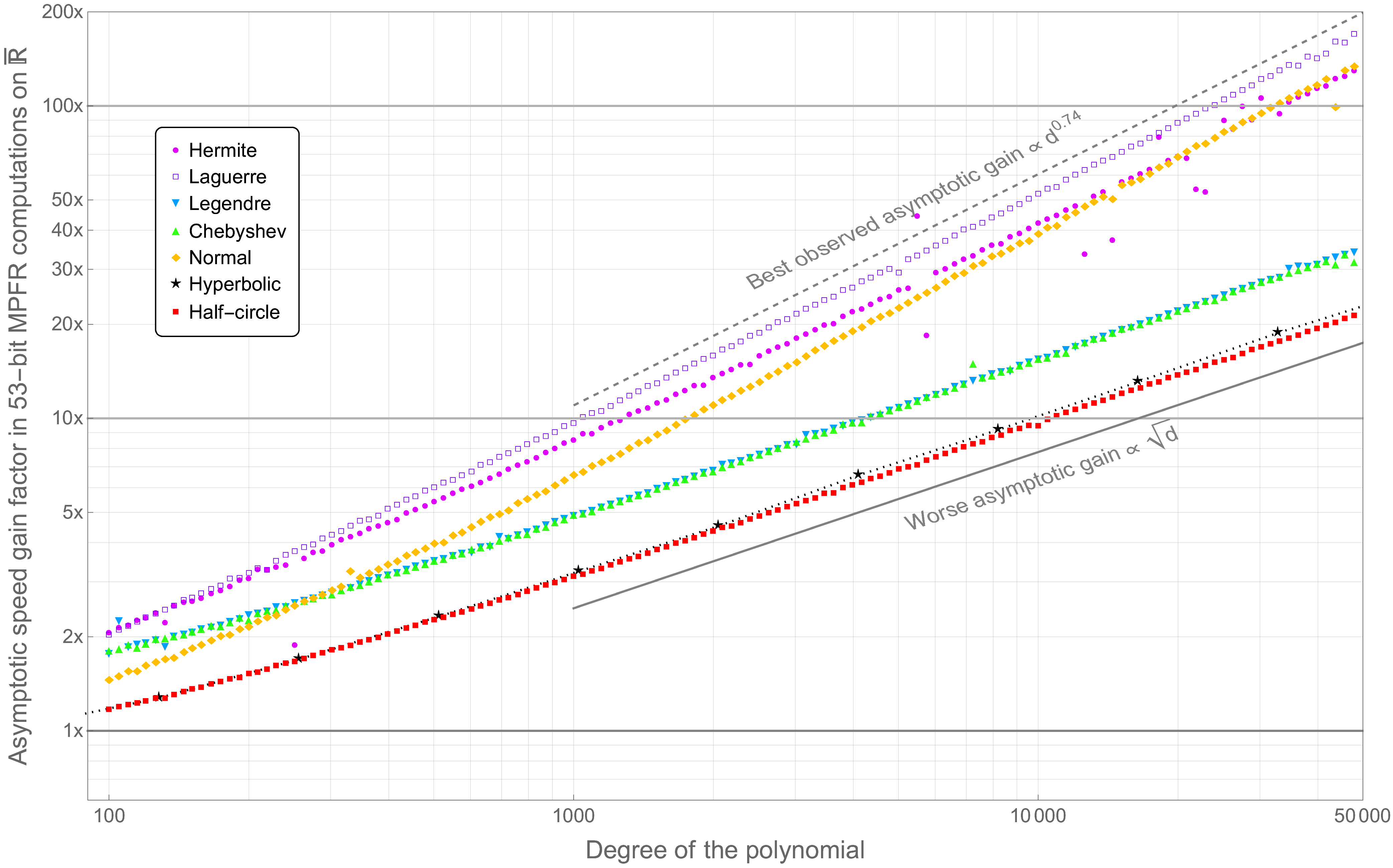
If the polynomial is evaluated repeatedly (which is what FPE is designed for), the preprocessing overhead becomes negligible (see Figure 19) and the asymptotic gain obtained by FPE becomes substantial. Speedup in excess of $\times 10$ occurs for some families like Hermite or Laguerre for degrees as low as 1000 (see Figure 18). In accordance with Theorem 4, if the degree is high enough, the speed gain is bounded from below by $O(\sqrt{d/\log_{2}d})$ , which is observed in practice (see Figures 20 and 21).

In the best cases (Laguerre and Hermite; see Figure 21), the complexity of the FPE evaluation scales, in practice, as $O(d^{0.26})$ along the real line and $O(d^{0.28})$ on the Riemann sphere. In our data range, this complexity is consistent with $O(\log^{2}d)\pm 10\%$ , which is the theoretical bound suggested by the last example of Section 4.4. Note that Figure 20 also hints that, in general, the exponent of the scaling law of the complexity does not depend on the precision used for the computations. Finally, let us point out that Chebychev, Legendre and Hermite polynomials are mildly lacunary (alternately odd or even); the others are not.

Sorting the polynomial families by increasing asymptotic gain as in Figure 18 and 21 is effectively a way of measuring the complexity in the variability of the scales of the coefficients. As explained in Section 5.3, the slowest case is that of the half-circle family. Similarly, the hyperbolic polynomials are slow to evaluate from their coefficients because of systematic compensations among monomials on the Mandelbrot set, which represents a substantial part of the Riemann sphere (about 29%). On the contrary, if $\wideparen{E}_{P}$ is composed of only a few segments, there will be very few values of $|z|$ for which massive compensations among monomials can occur; in this case, the FPE algorithm produces a very parsimonious representation of the polynomial (see Section 7.1), which in turn is responsible for extreme speed gains.

Most polynomial families behave qualitatively the same on $\overline{\mathbb{C}}$ , $\overline{\mathbb{R}}$ and on the unit disk. The only substantial anomaly in this classification occurs with the normal family (both real and complex), which is asymptotically evaluated significantly faster on $\overline{\mathbb{R}}$ than on $\overline{\mathbb{C}}$ : for a polynomial of degree $30\,000$ and a precision of 53 bits MPFR, FPE evaluations are asymptotically 100 times faster than Hörner’s on the real line but only 30 times faster on the Riemann sphere (see Figure 21). A reasonable explanation beyond the fact that real powers are easier to compute than complex ones, is the fact that the roots of normal polynomials accumulate uniformly along the unit circle (Hammersley’s theorem [Ham56], [SZ03]); therefore, one may expect fewer cancelations along the real line than for other families. However, the anisotropic example at the end of Section 5.3 suggests caution and further studies would be required to confirm this explanation. In particular, the reason why the evaluation time of the normal family on the Riemann sphere fails to obey a power law contrary to all other families is not clear.

Our implementation [MV22] handles both hardware number formats FP32, FP64 or FP80 and arbitrary-precision MPFR floating point numbers [MPFR]. The main limitation of hardware formats is the short range of exponents: roughly speaking, one can only represent numbers whose absolute value lies between $10^{\pm 38}$ with FP32 numbers and between $10^{\pm 308}$ with FP64 numbers. Concretely, this means it is simply impossible to compute a monomial $z^{n}$ in FP64 when $|z|\geq 2$ and $n>1024$ . The FP80 format provides a slightly more comfortable range between $10^{-4\,951}$ and $10^{4\,932}$ , but it is still not enough to handle polynomials of degree 50 000 as in our benchmark.

In the range of exponents where a comparison was possible, hardware numbers behave about 4 times faster than 53-bit MPFR numbers; however, the gain factor of FPE over Hörner obeys the same scaling law as for MPFR. In practice, the sweet spot for using the FPE algorithm with FP80 numbers is for polynomials of degree 1 000 to 5 000 and $|z|<10$ . When using MPFR numbers, this range is extended to essentially any degree above 100 with almost no practical limitation on $|z|$ .

The last crucial part in our benchmarks is the question of the accuracy of the FPE algorithm, which is guaranteed by Theorem 3. To put it to the test, we systematically computed a 600-bit evaluation of our polynomials with a Hörner scheme, which served as a reference value. For each benchmarked precision (up to 304 bits), the outputs of both Hörner and FPE algorithms with the current precision were compared to the reference value to identify the absolute computation error.

The most significant data that can be extracted from this computation is the accuracy bias, defined as the difference of the number of exact bits between the two algorithms, which is presented in Figure 22. The practical conclusion is that the values computed either by FPE or by Hörner are essentially identical, up to 1 exact bit. Of course, when cancelations occur, the displayed result may differ by many bits, but the divergence only affects the non significant bits at the end.

Based on this extensive benchmark, we can now confirm, in practice, that the FPE algorithm holds the promise of Theorems 3 and 4 and performs as accurately as Hörner, only faster.

Let us conclude this section by pointing out that our implementation of FPE provides additional tools for analyzing polynomial evaluations like the proportion of leading monomials at a given evaluation point (see Figure 14). Similarly, the localization of cancelations in the evaluation process can easily be deduced from the output files (see Figure 23), which may guide practical decisions to ensure the precision of subsequent computations.

We hope that the ideas presented in this article will inspire future developments, either theoretical or applied. We also thank the reader for reaching this point.

Appendix A Proof of the geometric statements

In this appendix, we prove the geometric results stated in Section 3.

The proof of Theorem 1 is based on two complementary geometric constructions and is split into several lemmas. In Lemma 20 we show the existence of a segment $[A(\tau)B(\tau)]$ in $S(f,\delta)$ of maximal length and of slope $\tau=\tan\theta$ . This segment touches the graph of $f-\delta$ in a “tangent” way (in the convex sense, i.e. as a subderivative).

In Lemma 21 we express the main integral from Theorem 1 in terms of $x_{R}-x_{L}$ where $x_{L}$ and $x_{R}$ are the respective abscissae of $A(\tau)$ and $B(\tau)$ . Next, we make an alternative geometric construction of $x_{R}$ and $x_{L}$ based on area computations. This second construction is the key to Lemma 22 where we estimate the diagonal of a square built upon the graph of $f^{\prime}$ . A change of variable in the plane (Lemma 23) allows us to collect all the prior estimates and leads to the proof of the upper bound in Theorems 1 and 2. Finally, we obtain the lower bounds by constructing explicit examples.

A.1 First geometric construction based on the graph of $f$

Let us start by presenting the construction in a simple case.

A typical example.

For now, we suppose $f\in C^{2}([0,1])$ with $f^{\prime\prime}(x)<0$ for all $x\in(0,1)$ and we single out $x_{0}\in(0,1)$ . The line of slope $f^{\prime}(x_{0})$ and passing through the point $(x_{0},f(x_{0})-\delta)$ is tangent to the graph of $f-\delta$ . This line intersects the graph of $f$ in at most two points $A$ and $B$ , one on each side of $x_{0}$ . Indeed, the points of intersection with the graph of $f$ correspond to the solutions of the equation

f(x_{0})-\delta+f^{\prime}(x_{0})(x-x_{0})=f(x)

(59)

i.e. $F(x)=-\delta$ , where $F(x)=f(x)-f(x_{0})-f^{\prime}(x_{0})(x-x_{0})$ . The function $F$ is of class $C^{2}([0,1])$ and $F^{\prime\prime}(x)=f^{\prime\prime}(x)<0$ for all $x\in(0,1)$ , thus $F$ is concave. Therefore $F^{\prime}(x)>0$ if $x<x_{0}$ , $F(x_{0})=F^{\prime}(x_{0})=0$ and $F^{\prime}(x)<0$ if $x>x_{0}$ . Consequently, there exist at most two points, one on each side of $x_{0},$ such that $F(x)=-\delta.$ When they exist, we denote them by $0\leq x_{L}<x_{0}<x_{R}\leq 1.$ When they do not, we simply take respectively $x_{L}=0$ or $x_{R}=1$ . In Figure 6, the common abscissa of the points $A$ , $A^{\prime}$ is $x_{L}$ while that of $B$ , $B^{\prime}$ is $x_{R}$ .

General case.

Let us now come back to the general setting where $f$ is concave, but not necessarily of class $C^{2}([0,1])$ . The next statement extends the simpler case presented in the previous paragraph. It is essentially an elementary version of F. Riesz’s rising sun lemma [Rie32] in a concave setting.

Lemma 20.

For any real number $\tau\in\mathbb{R}$ , there exists a unique segment $[A(\tau)B(\tau)]$ of maximal length, of slope $\tau=\tan\theta$ , contained in the strip $S(f,\delta)$ and that touches the graph of $f-\delta$ in a tangent way in the convex sense.

We denote by $g(x_{0}\pm 0)$ or $g(x_{0}^{\pm})$ the sided limits of a function $g$ :

g(x_{0}\pm 0)=\lim\limits_{\begin{subarray}{c}{x\to x_{0}}\\ {\pm(x-x_{0})>0}\end{subarray}}g(x)\,.

A segment $[AB]$ of slope $\tan\theta$ is said to be tangent in the convex sense to the graph of $g\in\mathcal{C}$ if, at any contact point $(x_{0},g(x_{0}))\in[AB]$ , one has $g^{\prime}(x_{0}+0)\leq\tan\theta\leq g^{\prime}(x_{0}-0)$ . If $g$ is smooth, then $g^{\prime}(x_{0})=\tan\theta$ . If an endpoint $x_{0}\in\{0,1\}$ is a contact point, then the requirement is lightened respectively to $\tan\theta\geq g^{\prime}(0^{+})$ or $\tan\theta\leq g^{\prime}(1^{-})$ .

The abscissa of the endpoints of the maximal segment $[A(\tau)B(\tau)]$ will be respectively denoted by $x_{L}(\tau)$ for the left side and $x_{R}(\tau)$ for the right side.

Proof.

As $f$ is a concave function, it is continuous, it is differentiable almost everywhere, and its derivative is decreasing. Even when the derivative is not continuous at a point, it necessarily has left and right limits. Therefore it has at most a countable number of jump points.

Let us first construct the segment $[A(\tau)B(\tau)]$ . For any $\tau\in\mathbb{R}$ , the concave function $f(x)-\tau x$ presents a maximum $m_{\tau}$ in $[0,1]$ , which is reached on some non-empty compact sub-interval $J_{\tau}\subset[0,1]$ (usually a singleton). The function $f(x)-\tau x$ is monotone on each of the connected components of $[0,1]\backslash J_{\tau}$ . As a consequence, the set

I(\tau,\delta)=\{x\in[0,1]\,;\,f(x)-\tau x\geq m_{\tau}-\delta\}

is an interval increasing in $\delta$ that contains $J_{\tau}=I(\tau,0)$ . Let us define

\begin{gathered}x_{L}(\tau)=\inf I(\tau,\delta)\,,\qquad x_{R}(\tau)=\sup I(\tau,\delta)\,.\end{gathered}

(60)

For any $x_{0}\in J_{\tau}$ , one has $m_{\tau}=f(x_{0})-\tau x_{0}$ and the line of equation $y=y_{\tau}(x)$ with

y_{\tau}(x)=f(x_{0})-\delta+\tau(x-x_{0})=\tau x+(m_{\tau}-\delta)

does not depend on the actual choice of $x_{0}$ within $J_{\tau}$ . Let us define

A(\tau)=(x_{L}(\tau),y_{\tau}(x_{L}(\tau)))\,,\hskip 20.00003ptB(\tau)=(x_{R}(\tau),y_{\tau}(x_{R}(\tau)))\,.

(61)

By definition (60), for all $x\in[x_{L}(\tau),x_{R}(\tau)]=I(\tau,\delta)$ , one has $f(x)+\delta\geq m_{\tau}+\tau x\geq f(x)$ , thus the segment $[A(\tau)B(\tau)]$ is of slope $\tau$ and is included in $S(f,\delta)$ .

Conversely, any segment $[AB]$ of slope $\tau$ included in $S(f,\delta)$ is supported by a line of equation $y=\tau x+\beta$ and must satisfy (denoting by $x_{A}$ , $x_{B}$ the abscissa of $A$ and $B$ )

\forall x\in[x_{A},x_{B}],\hskip 20.00003ptf(x)\geq\tau x+\beta\geq f(x)-\delta\hskip 10.00002pt\textit{i.e.}\penalty\ \hskip 10.00002pt\beta+\delta\geq f(x)-\tau x\geq\beta\,.

(62)

Let us show that $x_{B}-x_{A}\leq x_{R}(\tau)-x_{L}(\tau)$ .

If $\beta\geq m_{\tau}-\delta$ (i.e. $[AB]$ is above $[A(\tau)B(\tau)]$ ) then $f(x_{A})-\tau x_{A}\geq\beta\geq m_{\tau}-\delta$ ; the monotony of $f(x)-\tau x$ outside $J_{\tau}$ and the definition of $x_{L}(\tau)$ imply $x_{L}(\tau)\leq x_{A}$ . Similarly, one has $x_{B}\leq x_{R}(\tau)$ . In other words, one has

[x_{A},x_{B}]\subset[x_{L}(\tau),x_{R}(\tau)]\,.

If $\beta<m_{\tau}-\delta$ , the constraint (62) cannot be satisfied for $x\in J_{\tau}$ because

\forall x\in J_{\tau},\hskip 10.00002ptf(x)-\tau x=m_{\tau}>\beta+\delta\,,

thus $[x_{A},x_{B}]$ is a subset of $[0,1]\backslash J_{\tau}$ . The concavity of $f(x)-\tau x$ implies that one can increase $x_{B}-x_{A}$ by shifting the interval towards $J_{\tau}$ . More precisely, let us assume for example that $[x_{A},x_{B}]$ is on the right side of $J_{\tau}$ and that $x_{R}(\tau)<1$ (otherwise nothing needs to be proved). The inclusion $[AB]\subset S(f,\delta)$ implies

f(x_{A})-\tau x_{A}-\delta\leq\beta\leq f(x_{B})-\tau x_{B}\,.

(63)

The function $\tau-f^{\prime}$ is defined almost everywhere and is positive and increasing on the right-hand side of $J_{\tau}$ . The inequality (63) can thus be rephrased

\int_{x_{A}}^{x_{B}}\tau-f^{\prime}(x)dx\leq\delta\,.

Similarly, for any $x_{0}\in J_{\tau}$ , one has $f(x_{0})-\tau x_{0}=m_{\tau}$ and $x_{R}(\tau)<1$ implies :

\int_{x_{0}}^{x_{R}(\tau)}\tau-f^{\prime}(x)dx=m_{\tau}-\left(f(x_{R})-\tau x_{R}(\tau)\right)=\delta\,.

If $x_{A}\geq x_{R}(\tau)$ then the smaller integrand on $[x_{0},x_{R}(\tau)]$ implies $x_{R}(\tau)-x_{0}\geq x_{B}-x_{A}$ . If $x_{A}<x_{R}(\tau)$ , the integrals on $[x_{A},x_{R}(\tau)]$ cancel out, therefore

\int_{x_{R}(\tau)}^{x_{B}}\tau-f^{\prime}(x)dx\leq\int_{x_{0}}^{x_{A}}\tau-f^{\prime}(x)dx

and thus $x_{A}-x_{0}\geq x_{B}-x_{R}(\tau)$ . In both cases, $x_{R}(\tau)-x_{L}(\tau)\geq x_{R}(\tau)-x_{0}\geq x_{B}-x_{A}$ .

This proves that the maximal length is obtained for $\beta=m_{\tau}-\delta$ . As the values of the projection of $A,B$ on the $x$ -axis are unique, the equations (60)-(61) ensure that the segment $[A(\tau)B(\tau)]$ is unique. ∎

The quantity that interests us for Theorem 1 is obviously related to this first geometric construction.

Lemma 21.

With the notations of Theorem 1, we have

\int_{-\frac{\pi}{2}}^{\frac{\pi}{2}}L(f,\delta,\theta)\cos\theta\,d\theta=\int_{-\infty}^{+\infty}\frac{x_{R}(y)-x_{L}(y)}{1+y^{2}}\,dy\,.

(64)

We also have

\int_{-\frac{\pi}{2}}^{\frac{\pi}{2}}L(f,\delta,\theta)\cos^{2}\theta\,d\theta=\int_{-\infty}^{+\infty}\frac{x_{R}(y)-x_{L}(y)}{(1+y^{2})^{3/2}}\,dy

(65)

and for any positive measurable weight $\omega$ on $\left[-\frac{\pi}{2},\frac{\pi}{2}\right]$ :

\int_{-\frac{\pi}{2}}^{\frac{\pi}{2}}L(f,\delta,\theta)\,\omega(\theta)\,d\theta=\int_{-\infty}^{+\infty}\frac{x_{R}(y)-x_{L}(y)}{\sqrt{1+y^{2}}}\>\omega(\arctan y)\,dy\,.

(66)

Proof.

The definition (61) ensures that the length of the projection on the $x$ -axis of the segment $[A(\tau)B(\tau)]$ is $L(f,\delta,\theta)\cos\theta=x_{R}(\tan\theta)-x_{L}(\tan\theta)$ . The identities are then obtained by the change of variable $y=\tan\theta.$ ∎

A.2 A second geometric construction based on the graph of $f^{\prime}$

We are now going to provide a second geometric construction of $x_{L}(\tau)$ , $x_{R}(\tau)$ . We consider the graph of $f^{\prime}$ and we complete it to a continuous curve in the following way. At a jump point we add the vertical segment that joins the left and the right limits. If $f^{\prime}(0^{+})<\infty$ then we add the half-line $\{0\}\times[f^{\prime}(0^{+}),\infty)$ . Similarly, if $f^{\prime}(1^{-})>-\infty,$ we add the half-line $\{1\}\times(-\infty,f^{\prime}(1^{-})]$ . We thus obtain a continuous curve, which we denote by $\gamma_{f^{\prime}}$ , that contains the graph of $f^{\prime}$ , whose projection on the $x$ -axis contains $]0,1[$ and is included in $[0,1]$ and whose projection on the $y$ -axis is $\mathbb{R}$ .

Let us introduce

\Gamma_{f^{\prime}}^{\pm}=\left\{(x,y)\in[0,1]\times\mathbb{R}\,;\,\exists y^{\prime}\text{ such that }\pm(y-y^{\prime})\geq 0\text{ and }(x,y^{\prime})\in\gamma_{f^{\prime}}\right\}\,.

The sets $\Gamma_{f^{\prime}}^{\pm}$ are the closed subsets of the strip $[0,1]\times\mathbb{R}$ that are respectively above and below $\gamma_{f^{\prime}}$ . For every $y_{0}\in\mathbb{R}$ we consider

x_{0}^{-}=\min\left\{x\in[0,1]\,;\,(x,y_{0})\in\gamma_{f^{\prime}}\right\}\hskip 10.00002pt\text{and}\hskip 10.00002ptx_{0}^{+}=\max\left\{x\in[0,1]\,;\,(x,y_{0})\in\gamma_{f^{\prime}}\right\}\,.

The segment $\{(x,y_{0})\,;\,x_{0}^{-}\leq x\leq x_{0}^{+}\}$ is the intersection between $\gamma_{f^{\prime}}$ and the horizontal line $y=y_{0}$ ; it reduces to a point when $x_{0}^{+}=x_{0}^{-}$ . We now build a family of “triangles” whose hypotenuse rests on $\gamma_{f^{\prime}}$ and that collapse on the segment $[x_{0}^{-},x_{0}^{+}]\times\{y_{0}\}$ (see Figure 25). For $x\in[0,1]$ , let

T_{f^{\prime}}(y_{0};x)=\begin{cases}\Gamma_{f^{\prime}}^{-}\cap\left\{(x^{\prime},y)\,;\,x\leq x^{\prime}\leq x_{0}^{-}\text{ and }y\geq y_{0}\right\}&\text{if }x<x_{0}^{-},\\ \{x,y_{0}\}&\text{if }x\in[x_{0}^{-},x_{0}^{+}],\\ \Gamma_{f^{\prime}}^{+}\cap\left\{(x^{\prime},y)\,;\,x_{0}^{+}\leq x^{\prime}\leq x\text{ and }y\leq y_{0}\right\}&\text{if }x>x_{0}^{+}.\end{cases}

The continuity of $\gamma_{f^{\prime}}$ implies that the area $|T_{f^{\prime}}(y_{0};x)|$ of this triangle is a continuous function of $x$ and the monotonicity of $f^{\prime}$ implies that the area vanishes along $[x_{0}^{-},x_{0}^{+}]$ and is respectively strictly decreasing on $[0,x_{0}^{-}]$ and strictly increasing on $[x_{0}^{+},1]$ .

We are interested in the two points where either the area of the triangle equals $\delta$ or the triangle hits the edge of the strip:

	$\displaystyle\widetilde{x_{L}}(y_{0})$	$\displaystyle=\inf\left\{x\in[0,x_{0}^{-}]\,;\,\|T_{f^{\prime}}(y_{0};x)\|\leq\delta\right\}\,,$
	$\displaystyle\widetilde{x_{R}}(y_{0})$	$\displaystyle=\sup\left\{x\in[x_{0}^{+},1]\,;\,\|T_{f^{\prime}}(y_{0};x)\|\leq\delta\right\}\,.$

Let us prove that $\widetilde{x_{L}}(y_{0})=x_{L}(y_{0})$ and $\widetilde{x_{R}}(y_{0})=x_{R}(y_{0})$ , i.e. they are the same values as the ones defined by (60). Using elementary calculus, we know that the area of the triangle is

|T_{f^{\prime}}(y_{0};x)|=\begin{cases}\displaystyle\int_{x}^{x_{0}^{-}}\left(f^{\prime}(x)-y_{0}\right)dx=-(x_{0}^{-}-x)y_{0}+f(x_{0}^{-})-f(x)&\text{if }x<x_{0}^{-},\\[6.45831pt] \displaystyle\int_{x_{0}^{+}}^{x}\left(y_{0}-f^{\prime}(x)\right)dx=(x-x_{0}^{+})y_{0}+f(x_{0}^{+})-f(x)&\text{if }x>x_{0}^{+}.\end{cases}

The conditions defining $\widetilde{x_{L}}(y_{0})$ and $\widetilde{x_{R}}(y_{0})$ thus boil down to

x\in[\widetilde{x_{L}}(y_{0}),\widetilde{x_{R}}(y_{0})]\hskip 10.00002pt\Longleftrightarrow\hskip 10.00002ptf(x)-y_{0}x\geq f(x_{0}^{\pm})-y_{0}x_{0}^{\pm}-\delta\,.

Note that, by definition, $f(x)-y_{0}x$ is constant on $[x_{0}^{-},x_{0}^{+}]$ and one recovers (60) with $\tau=y_{0}$ , $m_{\tau}=f(x_{0}^{\pm})-y_{0}x_{0}^{\pm}$ and $[x_{0}^{-},x_{0}^{+}]=J_{\tau}$ from the proof of Lemma 20.

We now have two equivalent constructions of $x_{L}(y)=\widetilde{x_{L}}(y)$ and $x_{R}(y)=\widetilde{x_{R}}(y)$ for every $y\in\mathbb{R}$ . The second construction ensures that the maps $y\mapsto x_{R}(y)$ and $y\mapsto x_{L}(y)$ are continuous and decreasing on $\mathbb{R}$ . They are strictly decreasing respectively when $x_{L}(y)>0$ and $x_{R}(y)<1$ . We denote by $\gamma_{L}(\delta)=\{(x_{L}(y),y)\,;\,y\in\mathbb{R}\}$ and $\gamma_{R}(\delta)=\{(x_{R}(y),y)\,;\,y\in\mathbb{R}\}$ the two curves that are “offset” from $\gamma_{f^{\prime}}$ by a triangular area of $\delta$ (see Figure 25).

Lemma 22.

For every $y\in\mathbb{R}$ let us construct the unique square with an upper-right corner at $(x_{R}(y),y)\in\gamma_{R}(\delta)$ and a lower-left corner on $\gamma_{L}(\delta)$ . The area of this square is smaller than $2\delta$ and therefore its diagonal is smaller than $2\sqrt{\delta}$ .

Proof.

The construction of the square is obvious. The curve $\gamma_{L}$ is below the curve $\gamma_{f^{\prime}}$ , which is itself below $\gamma_{R}$ . As $y\mapsto x_{L}(y)$ is decreasing, the curve $\gamma_{L}$ intersects a line of slope $\pi/4$ passing through $(x_{R}(y),y)$ in a unique point whose coordinates are, by definition, of the form $(x_{L}(y^{\prime}),y^{\prime})$ for some $y^{\prime}<y$ . The two points $(x_{R}(y),y)$ and $(x_{L}(y^{\prime}),y^{\prime})$ are the opposite corners of a square, which we will denote by $Q(y^{\prime},y)$ in the rest of this proof; see Figure 26 (left). Notice that this square is always included in the strip between the curves $\gamma_{L}$ and $\gamma_{R}.$

The curve $\gamma_{f^{\prime}}$ can only enter the square on its left or upper side and can only leave the square on its right or bottom side, as seen in Figure 26 (right). In all 4 cases, one has

	$\displaystyle Q(y^{\prime},y)\cap\Gamma_{f^{\prime}}^{-}$	$\displaystyle\subset T_{f^{\prime}}(y^{\prime};x_{L}(y^{\prime}))\,,$
	$\displaystyle Q(y^{\prime},y)\cap\Gamma_{f^{\prime}}^{+}$	$\displaystyle\subset T_{f^{\prime}}(y;x_{R}(y))\,,$

thus $Q(y^{\prime},y)\subset T_{f^{\prime}}(y^{\prime};x_{L}(y^{\prime}))\cup T_{f^{\prime}}(y;x_{R}(y))$ . As this is a measurably disjoint union of 2 triangles of area at most $\delta$ (the area of $\gamma_{f^{\prime}}$ is zero), the area of the square $Q(y^{\prime},y)$ is smaller than or equal to $2\delta$ and consequently its diagonal is smaller than or equal to $2\sqrt{\delta}$ . ∎

From this point on, the idea is to use Fubini’s theorem to slice the strip between the curves $\gamma_{L}$ and $\gamma_{R}$ along the first diagonal. In this direction, according to Lemma 22, the girth does not exceed $2\sqrt{\delta}$ and the decay of the integrands will ensure the integrability. We prepare this computation by a suitable change of variable.

Lemma 23.

Let us denote by $\Omega$ the strip between the curves $\gamma_{L}$ and $\gamma_{R}$ . One has

\int_{-\frac{\pi}{2}}^{\frac{\pi}{2}}L(f,\delta,\theta)\cos\theta\,d\theta=\iint_{\Omega}\frac{dxdy}{1+y^{2}}=\iint_{\Omega^{\prime}}\frac{dx_{1}dx_{2}}{1+\frac{1}{2}(x_{1}-x_{2})^{2}}\,,

(67)

\int_{-\frac{\pi}{2}}^{\frac{\pi}{2}}L(f,\delta,\theta)\cos^{2}\theta\,d\theta=\iint_{\Omega}\frac{dxdy}{(1+y^{2})^{3/2}}=\iint_{\Omega^{\prime}}\frac{dx_{1}dx_{2}}{\left(1+\frac{1}{2}(x_{1}-x_{2})^{2}\right)^{3/2}}\,,

(68)

where $\Omega^{\prime}=R_{\pi/4}\left(\Omega\right)$ is the image of $\Omega$ by the rotation of angle $\pi/4$ that maps $(1/2,0)$ to the origin. More generally, for any positive weight $\omega\in L^{1}_{\text{loc}}\left(-\frac{\pi}{2},\frac{\pi}{2}\right)$ such that $\omega\left(\pm(\frac{\pi}{2}-t)\right)\leq C\left|\ln t\right|^{-\beta}$ with $\beta>1$ as $t\to 0^{+}$ , one has

\int_{-\frac{\pi}{2}}^{\frac{\pi}{2}}L(f,\delta,\theta)\,\omega(\theta)\,d\theta=\iint_{\Omega}\frac{\omega(\arctan y)}{\sqrt{1+y^{2}}}\,dxdy=\iint_{\Omega^{\prime}}\frac{\omega\left(\arctan\frac{x_{2}-x_{1}}{\sqrt{2}}\right)}{\sqrt{1+\frac{1}{2}(x_{1}-x_{2})^{2}}}\,dx_{1}dx_{2}\,.

(69)

Proof.

In view of Lemma 21 and the geometric construction above (and because $x_{R}$ and $x_{L}$ are continuous), we can re-write the integral with Fubini’s theorem, which gives the first identities. The change of variable is the composition of a translation by $(-1/2,0)$ that moves the domain $\Omega$ into the strip $[-1/2,1/2]\times\mathbb{R}$ followed by a rotation around the origin of angle $\frac{\pi}{4}$ . We denote by $\Omega^{\prime}$ the image of $\Omega$ by this isometry (see Figure 27). The new coordinates $(x_{1},x_{2})\in\Omega^{\prime}$ are thus related to the old ones by

x=\frac{1}{2}+\frac{1}{\sqrt{2}}(x_{1}+x_{2})\hskip 20.00003pt\text{and}\hskip 20.00003pty=\frac{1}{\sqrt{2}}(x_{2}-x_{1})\,.

The Jacobian determinant is obviously equal to $1$ . For (69), the assumption on the weight $\omega$ ensures that $\omega(\arctan y)\leq C\ln^{-\beta}|y|$ at infinity, which in turn ensures the integrability thanks to Bertrand’s criterion. ∎

Remark 24.

In Section 4, we apply (69) with a bounded regular even weight that decreases away from zero and vanishes at the endpoints $\pm\pi/2$ . In particular, the assumption will be satisfied because $\omega\left(\frac{\pi}{2}-t\right)\leq C|t|\ll\left|\ln t\right|^{-2}$ as $t\to 0$ .

A.3 Proof of the upper bounds in Theorems 1 and 2

Using the previous lemmas we can now prove the upper bounds stated in Theorems 1 and 2. As $\Omega$ is a subset of $[0,1]\times\mathbb{R}$ , $\Omega^{\prime}$ lies between the lines $(\pm\frac{\sqrt{2}}{2},0)+\mathbb{R}\cdot(1,-1)$ . Therefore,

\forall(x_{1},x_{2})\in\Omega^{\prime},\hskip 20.00003pt-\frac{\sqrt{2}}{2}-x_{1}\leq x_{2}\leq\frac{\sqrt{2}}{2}-x_{1}\,.

Consequently,

-2\left(\frac{\sqrt{2}}{4}+x_{1}\right)\leq x_{2}-x_{1}\leq 2\left(\frac{\sqrt{2}}{4}-x_{1}\right).

(70)

Moreover, Lemma 22 ensures that for every $x_{1}\in\mathbb{R}$ , the length of any vertical section of $\Omega^{\prime}$ is bounded in the following way:

\forall x_{1}\in\mathbb{R},\hskip 20.00003pt\left|\{x_{2}\,;\,(x_{1},x_{2})\in\Omega^{\prime}\}\right|\leq 2\sqrt{\delta}\,.

(71)

We now split $\Omega^{\prime}$ into three parts $\Omega^{\prime}=\Omega^{\prime}_{\text{I}}\cup\Omega^{\prime}_{\text{II}}\cup\Omega^{\prime}_{\text{III}}$ with

\Omega^{\prime}_{\text{I}}=\Omega^{\prime}\cap\left\{x_{1}\leq-\frac{\sqrt{2}}{4}\right\},\hskip 10.00002pt\Omega^{\prime}_{\text{II}}=\Omega^{\prime}\cap\left\{x_{1}\geq\frac{\sqrt{2}}{4}\right\}\hskip 10.00002pt\text{and}\hskip 10.00002pt\Omega^{\prime}_{\text{III}}=\Omega^{\prime}\cap\left\{-\frac{\sqrt{2}}{4}<x_{1}<\frac{\sqrt{2}}{4}\right\}\,.

On $\Omega^{\prime}_{\text{I}}$ we have $\frac{\sqrt{2}}{4}+x_{1}\leq 0$ and all the terms that appear in the estimate (70) are positive. Taking the square of the left-hand side gives $1+2\left(x_{1}+\frac{\sqrt{2}}{4}\right)^{2}\leq 1+\frac{1}{2}(x_{2}-x_{1})^{2}$ and therefore

\iint_{\Omega^{\prime}_{\text{I}}}\frac{dx_{1}dx_{2}}{1+\frac{1}{2}(x_{1}-x_{2})^{2}}\leq\iint_{\Omega^{\prime}_{\text{I}}}\frac{dx_{1}dx_{2}}{1+2\left(x_{1}+\frac{\sqrt{2}}{4}\right)^{2}}\cdotp

Notice that the function to integrate on the right-hand side does not depend on $x_{2}$ . Using Fubini’s theorem and the estimate (71) we have

\iint_{\Omega^{\prime}_{\text{I}}}\frac{dx_{1}dx_{2}}{1+\frac{1}{2}(x_{1}-x_{2})^{2}}\leq 2\sqrt{\delta}\int_{-\infty}^{-\frac{\sqrt{2}}{4}}\frac{dx_{1}}{1+2\left(x_{1}+\frac{\sqrt{2}}{4}\right)^{2}}\,\cdotp

With a change of variable $t=\frac{1}{2}+\sqrt{2}x_{1}$ we obtain

\iint_{\Omega^{\prime}_{\text{I}}}\frac{dx_{1}dx_{2}}{1+\frac{1}{2}(x_{1}-x_{2})^{2}}\leq\frac{\pi}{\sqrt{2}}\,\sqrt{\delta}\,.

(72)

On $\Omega^{\prime}_{\text{II}}$ we have that $\frac{\sqrt{2}}{4}-x_{1}\leq 0$ and a similar computation to the one on $\Omega^{\prime}_{\text{I}}$ leads to

\iint_{\Omega^{\prime}_{\text{II}}}\frac{dx_{1}dx_{2}}{1+\frac{1}{2}(x_{1}-x_{2})^{2}}\leq 2\sqrt{\delta}\int_{\frac{\sqrt{2}}{4}}^{\infty}\frac{dx_{1}}{1+2\left(x_{1}-\frac{\sqrt{2}}{4}\right)^{2}}=\frac{\pi}{\sqrt{2}}\,\sqrt{\delta}\,.

(73)

On $\Omega^{\prime}_{\text{III}}$ , the decay of the integrand is negligible so we use $\frac{1}{1+\frac{1}{2}(x_{1}-x_{2})^{2}}\leq 1$ . The geometric estimate (71) of the length of the vertical slices provides

\iint_{\Omega^{\prime}_{\text{III}}}\frac{dx_{1}dx_{2}}{1+\frac{1}{2}(x_{1}-x_{2})^{2}}\leq 2\sqrt{\delta}\times 2\frac{\sqrt{2}}{4}=\sqrt{2\delta}\,.

(74)

We put together the estimates (72), (73), (74) into the expressions given by Lemma 23 and conclude that

\int_{-\frac{\pi}{2}}^{\frac{\pi}{2}}L(f,\delta,\theta)\cos\theta\,d\theta\leq(1+\pi)\sqrt{2\delta}\,.

Normalizing by $1/\pi$ gives (25) with the numerical constant $\frac{1+\pi}{\pi}\sqrt{2}\approx 1.86437$ . A similar computation can be performed for the second integral:

	$\displaystyle\int_{-\frac{\pi}{2}}^{\frac{\pi}{2}}L(f,\delta,\theta)\cos^{2}\theta\,d\theta$	$\displaystyle=\iint_{\Omega^{\prime}_{\text{I}}\cup\Omega^{\prime}_{\text{II}}\cup\Omega^{\prime}_{\text{III}}}\frac{dx_{1}dx_{2}}{\left(1+\frac{1}{2}(x_{1}-x_{2})^{2}\right)^{3/2}}$
		$\displaystyle\leq 2\sqrt{\delta}\left(2\times\int_{\frac{\sqrt{2}}{4}}^{\infty}\frac{dx_{1}}{\left(1+2\left(x_{1}-\frac{\sqrt{2}}{4}\right)^{2}\right)^{3/2}}+2\times\frac{\sqrt{2}}{4}\right).$

The right-hand side is equal to $3\sqrt{2\delta}\approx\pi\times 1.35047\sqrt{\delta}$ , as claimed by (26).

Similarly, for a general even and positive weight function $\omega$ on $\left(-\frac{\pi}{2},\frac{\pi}{2}\right)$ that is decreasing on $[0,\pi/2)$ , thanks to (70), one has on $\Omega^{\prime}_{\text{I}}\cup\Omega^{\prime}_{\text{II}}$ :

\omega\left(\arctan\frac{x_{2}-x_{1}}{\sqrt{2}}\right)\leq\omega\left(\arctan\left(\frac{1}{2}-\sqrt{2}\,|x_{1}|\right)\right).

The estimate (27) follows immediately, provided that the constant (28) is finite (e.g. under the assumptions stated in Lemma 23, which are recalled in Theorem 2). One can easily check that this estimate boils down to the previous (25) when $\omega(\theta)=\cos\theta$ and to (26) when $\omega(\theta)=\cos^{2}\theta$ .

A.4 Proof of the lower bounds in Theorem 1

We end this section with computations on particular cases that assert the quasi-optimality of the constants from Theorem 1. The best (i.e. highest) lower bound is given by the second example, however the others are instructive for getting a feel for which cases are the least favorable to our algorithm (see Section 4).

Example 1 :

If $f(x)=ax+b$ for some $a,b\in\mathbb{R}$ , then $S(f,\delta)$ is a parallelogram. Let us introduce $\alpha=\arctan(a)$ and $\theta_{0},\theta_{1}\in(0,\frac{\pi}{2})$ the geometric angles that the diagonals make with the long sides of the parallelogram. Let us reason with $a\geq 0$ as in Figure 28.

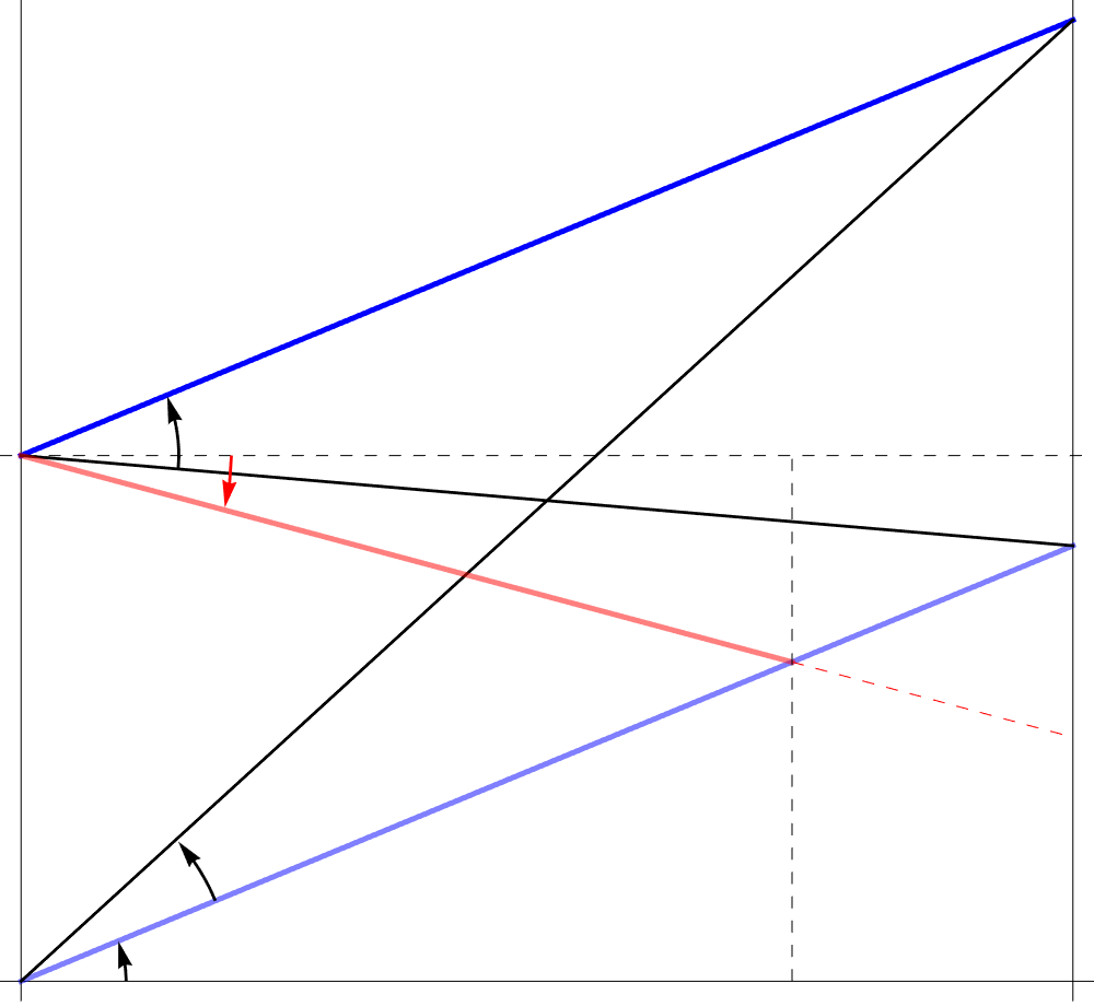
One has $\tan(\alpha+\theta_{0})=a+\delta$ and $\tan(\alpha-\theta_{1})=a-\delta$ and for $\theta\in(\alpha-\theta_{1},\alpha+\theta_{0})$ we have $L(f,\delta,\theta)\cos\theta=x_{R}(\theta)-x_{L}(\theta)=1.$ For $\theta\in\left(-\frac{\pi}{2},\alpha-\theta_{1}\right)$ the length of the projection $\ell=L(f,\delta,\theta)\cos\theta$ satisfies $\delta+\ell\tan(\theta)=\ell\tan(\alpha)$ , i.e. $\ell=\frac{\delta}{\tan\alpha-\tan\theta}\cdotp$ Similarly, for $\theta\in(\alpha+\theta_{0},\frac{\pi}{2})$ we have $L(f,\delta,\theta)\cos\theta=\frac{\delta}{\tan\theta-\tan\alpha}\cdotp$ Splitting the integral thus gives

\int_{-\frac{\pi}{2}}^{\frac{\pi}{2}}L(f,\delta,\theta)\cos\theta\,d\theta=\int_{-\frac{\pi}{2}}^{\alpha-\theta_{1}}\frac{\delta\,d\theta}{\tan\alpha-\tan\theta}+\theta_{0}+\theta_{1}+\int_{\alpha+\theta_{0}}^{\frac{\pi}{2}}\frac{\delta\,d\theta}{\tan\theta-\tan\alpha}\,\cdotp

This integral is easiest to compute when $a=\alpha=0$ i.e. when $f$ is a constant; in this case one has $\theta_{0}=\theta_{1}\simeq\delta$ and

\int_{-\frac{\pi}{2}}^{\frac{\pi}{2}}L(f,\delta,\theta)\cos\theta\,d\theta=2\left(\int_{0}^{\theta_{0}}1\,d\theta+\int_{\theta_{0}}^{\frac{\pi}{2}}\frac{\delta}{\tan\theta}\,d\theta\right)=2(\theta_{0}-\delta\log(\sin\theta_{0}))\,,

which is of leading order $-2\delta\ln(\delta)\ll\sqrt{\delta}$ . In the general case, one has

\theta_{0}+\theta_{1}=\arctan(a+\delta)-\arctan(a-\delta)=\frac{2\delta}{1+a^{2}}+O(\delta^{3})\,,

and a primitive

\int\frac{d\theta}{\tan\theta-\tan\alpha}=\frac{-a\theta+\log\left|(a-\tan\theta)\cos\theta\right|}{1+a^{2}}\,\cdotp

One thus obtains

\int_{-\frac{\pi}{2}}^{\frac{\pi}{2}}L(f,\delta,\theta)\cos^{2}\theta\,d\theta\leq\int_{-\frac{\pi}{2}}^{\frac{\pi}{2}}L(f,\delta,\theta)\cos\theta\,d\theta=-\frac{2\delta\log\delta}{1+a^{2}}+O(\delta)\ll\sqrt{\delta}\,.

(75)

Example 2 :

Let us consider $f(x)=\sqrt{x(1-x)}$ for $x\in[0,1]$ . The graph of $f$ is a half circle of radius $1/2$ ; the tangent at the origin is vertical. Assuming $\delta<1/2$ , we denote by $\theta_{0}\in(0,\frac{\pi}{2})$ the angle of the tangent to the graph of $f-\delta$ that passes through the origin and by $x_{0}$ the first coordinate of the tangence point. One has $\tan\theta_{0}=f^{\prime}(x_{0})$ and $f(x_{0})-\delta+(0-x_{0})\tan\theta_{0}=f(0)$ . A simple computation provides $x_{0}=\frac{4\delta^{2}}{1+4\delta^{2}}$ and $\theta_{0}=\arctan(\frac{1-4\delta^{2}}{4\delta})=\frac{\pi}{2}-4\delta+O(\delta^{2})$ .

For $\theta\in[-\theta_{0},\theta_{0}]$ the longest segment $[AB]\subset S(f,\delta)$ of angle $\theta$ has both of its ends on the graph of $f$ and is tangent to the graph of $f-\delta$ . Using the symmetry of the graph, one can assume that $\theta\geq 0$ . Let $(x_{\theta},f(x_{\theta})-\delta)$ denote the point where $[AB]$ is tangent to the graph of $f-\delta.$ As $\tan\theta=f^{\prime}(x_{\theta})=\frac{1-2x_{\theta}}{2\sqrt{x_{\theta}(1-x_{\theta})}}$ , the equation of $[AB]$ gives

4x_{\theta}^{2}-4x_{\theta}+\cos^{2}\theta=0.

As $\theta\geq 0$ and $x_{\theta}<\frac{1}{2}$ by symmetry, then $x_{\theta}=\frac{1}{2}(1-\sin\theta).$ The abscissae $x_{A}$ , $x_{B}$ of the endpoints satisfy $f(x_{\theta})-\delta+(x-x_{\theta})\tan\theta=f(x)$ , which is equivalent to

x^{2}-x(1-\sin\theta+\delta\sin 2\theta)+\frac{1}{4}(1-\sin\theta-2\delta\cos\theta)^{2}=0\,.

Their difference $x_{B}-x_{A}=L(f,\delta,\theta)\cos\theta$ is therefore given by $x_{B}-x_{A}=\sqrt{\Delta}$ where $\Delta$ denotes the discriminant, namely $\Delta=(1-\sin\theta+\delta\sin 2\theta)^{2}-(1-\sin\theta-2\delta\cos\theta)^{2}=4\delta\cos^{3}\theta(1-\delta\cos\theta)$ . Using a similar estimate on $[-\theta_{0},0]$ one gets the lower bounds

\frac{1}{\pi}\int_{-\frac{\pi}{2}}^{\frac{\pi}{2}}L(f,\delta,\theta)\cos\theta\,d\theta\geq\frac{4\sqrt{\delta}}{\pi}\int_{0}^{\theta_{0}}\sqrt{1-\delta\cos\theta}\cos^{3/2}\theta\,d\theta=C_{1}(\delta)\sqrt{\delta}

and

\frac{1}{\pi}\int_{-\frac{\pi}{2}}^{\frac{\pi}{2}}L(f,\delta,\theta)\cos^{2}\theta\,d\theta\geq\frac{4\sqrt{\delta}}{\pi}\int_{0}^{\theta_{0}}\sqrt{1-\delta\cos\theta}\cos^{5/2}\theta\,d\theta=C_{2}(\delta)\sqrt{\delta}\,.

When $\delta\ll 1$ , the contributions to the integrals outside $[-\theta_{0},\theta_{0}]$ are of a lower order. The dependence on $\delta$ of the lower bounds is illustrated in Figure 29.

The functions $C_{1}$ and $C_{2}$ are continuous and strictly decreasing, with

C_{1}(0)=\frac{4\sqrt{2}K(1/2)}{3\pi}>1.11283\,,\hskip 20.00003ptC_{2}(0)=\frac{12\sqrt{2}\Gamma(3/4)^{2}}{5\pi^{3/2}}>0.915311\,,

(76)

where $K$ and $\Gamma$ are classical special functions (respectively the complete elliptic integral of the first kind and the Gamma function).

See Section 5.3 for an adaptation of this example to polynomials that saturate the upper-bound on the complexity of the FPE algorithm, both theoretically and in practice.

Example 3 :

We study $f(x)=-a(x-\frac{1}{2})^{2}$ for $x\in[0,1]$ with $a>0$ and with $\delta<a/4$ . Notice the symmetry with respect to the line $x=1/2$ and that the maximum of $f-\delta$ is $-\delta$ and is superior to $f(0)=-a/4.$ We denote by $\theta_{0}\in(0,\frac{\pi}{2})$ the angle between the $x$ -axis and the line tangent to the graph of $f-\delta$ that passes through $(0,-a/4)$ and by $x_{0}$ the first coordinate of the point where this tangent intersects the graph of $f$ . Substituting $\tan\theta_{0}=f^{\prime}(x_{0})$ in the equation $f(x_{0})-\delta+(0-x_{0})\tan\theta_{0}=f(0)$ ensures that $x_{0}=\sqrt{\delta/a}$ and $\tan\theta_{0}=a-2\sqrt{a\delta}.$

For $\theta\in(0,\theta_{0})$ both ends of the longest segment $[AB]\subset S(f,\delta)$ of slope $\theta$ belong to the graph of $f$ and $[AB]$ is tangent to the graph of $f-\delta$ . As before, let $(x_{\theta},f(x_{\theta})-\delta)$ denote the point where $[AB]$ is tangent to the graph of $f-\delta$ and $x_{A}$ , $x_{B}$ the first coordinate of the endpoints. Then $f^{\prime}(x_{\theta})=\tan\theta$ gives $x_{\theta}=\frac{1}{2}-\frac{\tan\theta}{2a}$ and the equation of $[AB]$ implies that $x_{A}$ , $x_{B}$ satisfy

a\left(x-\frac{1}{2}\right)^{2}+\left(x-\frac{1}{2}\right)\tan\theta+\frac{\tan^{2}\theta}{4a}-\delta=0\,.

The difference $x_{B}-x_{A}=L(f,\delta,\theta)\cos\theta$ is thus given by $x_{R}-x_{L}=\sqrt{\Delta}/a$ with $\Delta=4a\delta$ . Using a similar estimate on $[-\theta_{0},0]$ one gets the lower bounds

\frac{1}{\pi}\int_{-\frac{\pi}{2}}^{\frac{\pi}{2}}L(f,\delta,\theta)\cos\theta\,d\theta\geq\frac{2}{\pi}\int_{0}^{\theta_{0}}2\sqrt{\frac{\delta}{a}}\,d\theta=\frac{4\sqrt{\delta}}{\pi\sqrt{a}}\arctan(a-2\sqrt{a\delta})\,,

\frac{1}{\pi}\int_{-\frac{\pi}{2}}^{\frac{\pi}{2}}L(f,\delta,\theta)\cos^{2}\theta\,d\theta\geq\frac{4\sqrt{\delta}}{\pi\sqrt{a}}\int_{0}^{\theta_{0}}\cos\theta\,d\theta=\frac{4\sqrt{\delta}}{\pi\sqrt{a}}\frac{a-2\sqrt{a\delta}}{\sqrt{1+(a-2\sqrt{a\delta})^{2}}}\,\cdotp

Notice that for $\delta=a/4$ the right-hand side vanishes. For $\delta\ll a/4$ , both bounds are of order $\sqrt{\delta}$ . The first constant is approximately $\frac{4\arctan(a)}{\pi\sqrt{a}}$ , whose maximum is $1.02288$ for $a\simeq 1.39175$ . The second constant becomes $\frac{4\sqrt{a}}{\pi(1+a^{2})}$ , whose maximum is $0.72559$ and is obtained for $a\simeq 0.57735$ .

Remark 25.

The case $a=1/2$ in Example 3 corresponds to $f^{\prime\prime}(x)\equiv\textendash 1$ for which the estimate from Lemma 22 is optimal (see Figure 26). However, this example does not saturate the inequalities (25)-(26).

Appendix B Index of notations

We provide here a short index of our notations. By default, we use the American standard names, notations and spellings.

Numbers

: $z=a+ib\in\mathbb{C}$ : complex numbers (with $a,b\in\mathbb{R}$ ).
: $\lfloor\cdot\rfloor$ and $\lceil\cdot\rceil$ : resp. floor and ceiling functions (round down/up to the next integer).
: $\ln x$ : natural logarithm.
: $\log_{b}x=\frac{\ln x}{\ln b}$ : base- $b$ logarithm (for complexity, the default base is $b=2$ ).
: $x\simeq y$ : the numbers $x$ and $y$ have a similar order of magnitude (used colloquially).
: $y\lesssim y$ : the order of magnitude of $x$ is smaller than or equal to that of $ys$ (used colloquially).

Asymptotic estimates

The asymptotic parameter $\sigma\to\sigma^{\ast}$ can be continuous or discrete and is given from context; the signs (or complex phase) of $A,B$ are irrelevant.

: $A=O(B)$ : there exists a bounded function $C(\sigma)$ such that $A(\sigma)=C(\sigma)B(\sigma)$ .
: $A\ll B$ : there exists a function $\varepsilon(\sigma)$ that tends to zero, such that $A(\sigma)=\varepsilon(\sigma)B(\sigma)$ .

Sets

: $\llbracket{m},{n}\rrbracket=\{m,m+1,\ldots,n-1,n\}$ : integer interval $[m,n]\cap\mathbb{Z}$ .
: $[a,b)$ : real-line interval, semi-open on the right side.
: $\overline{\mathbb{C}}=\mathbb{C}\cup\{\infty\}$ : Riemann Sphere.
: $\overline{\mathbb{R}}=\mathbb{R}\cup\{\infty\}$ : compaction of $\mathbb{R}$ into a circle.
: $\#E$ : cardinal of a finite set.
: $|E|$ : Lebesgue measure of a measurable set $E\subset\mathbb{R}^{n}$ .

Polynomials

: $\mathbb{K}[X]$ : set of polynomials with coefficients in the field $\mathbb{K}$ (typically $\mathbb{R}$ or $\mathbb{C}$ ).
: $\mathbb{K}[[X]]$ : set of formal series with coefficients in the field $\mathbb{K}$ .

Complexity

(see page 1)

: $\eval_{d}$ : arithmetic complexity of evaluating a polynomial of degree $d$ .
: $\eval_{d}(k)$ : arithmetic complexity of $k$ polynomial evaluations of degree $d$ .
: $\eval_{d}(k,p)$ : bit complexity of evaluating a polynomial of degree $d$ on $k$ evaluation points with a fixed precision of $p$ bits for all intermediary computations.
: $M(p)$ : bit complexity of one multiply-add of two floating-point numbers with precision $p$ .

Floating-point numbers

(see page 3)

: $\xi=\pm 2^{n}\times 0.1\xi_{1}\xi_{2}\ldots\xi_{p}$ : bit presentation of a floating point number.
: $\ulp(\xi)$ : unit in the last place (smallest increment possible of the $p$ -bit number $|\xi|$ ).

Floating-point representations of real and complex numbers

(see Section 2.4)

: $s(z)$ : scale of a complex number (page 6).
: $x=_{p}y$ : $x,y\in\mathbb{R}$ have the same floating-point representation with precision $p\in\mathbb{N}^{*}$ .
: $x\simeq_{p}y$ : the $p$ -bit floating-point representations of $x,y\in\mathbb{R}$ are identical or adjacent.
: $z\approx_{p}z^{\prime}$ : $z,z^{\prime}\in\mathbb{C}$ have similar $p$ -bits representations, reduced by phase-shift invariance; see (20).

Concave geometry

(see Section 3)

: subgraph : for a concave function $f$ , region of the $(x,y)$ -plane such that $y\leq f(x)$ .
: $S(f,\delta)$ : edge of the subgraph of $f$ of (vertical) thickness $\delta$ .
: $L(f,\delta,\theta)$ : maximal length of a segment of slope $\tan\theta$ contained in the strip $S(f,\delta)$ .
: Equation (34) : definition of $f$ and $\delta$ in the FPE Algorithm application case.

FPE Algorithm

(see Section 4)

: $E_{P}:\llbracket{0},{d}\rrbracket\rightarrow\mathbb{Z}\cup\{-\infty\}$ : scales of the coefficients of the polynomial $P$ .
: $\wideparen{E}_{P}:[0,d]\rightarrow\mathbb{R}\cup\{-\infty\}$ : concave cover of $E_{P}$ .
: $\lambda=\log_{2}|z|=-\tan\theta$ : dyadic scale of the evaluation point $z$ .
: $G_{p}$ , $B_{p}$ : list of a-priori good (resp. ignored) coefficients for a given precision $p$ .
: $\ell$ , $r$ : left/right edges to further reduce $G_{p}$ for a given $\lambda$ .
: $Q_{\lambda}(z)$ : reduced polynomial produced by the FPE algorithm.
: $\textrm{FPE}_{p}$ : new algorithm proposed in this article, for computations with a fixed precision $p$ .
: $\avg_{\overline{\mathbb{C}}}$ : average operator for $z$ uniformly distributed over $\overline{\mathbb{C}}$ .
: $\avg_{\overline{\mathbb{R}}}$ : average operator for $z$ uniformly distributed over $\overline{\mathbb{R}}$ .
: $\avg_{D(0,1)}$ : average operator for $z$ uniformly distributed over the unit complex disk.

Appendix C Listing of tasks implemented in [MV22]

In our implementation [MV22], the tasks listed in this section are called in the command line with FastPolyEval -task [arguments]. The first argument is systematically the precision of the computation, in bits. Use -task -help for more detailed informations.

Tools for generating and handling polynomials
-sum	computes the sum of two polynomials and writes the result to a CSV file
-diff	computes the difference of two polynomials
-prod	computes the product of two polynomials
-der	computes the derivative of a polynomial
-roots	computes the polynomial with a given list of roots
-Chebyshev	writes the coefficients of the Chebyshev polynomial
-Legendre	writes the coefficients of the Legendre polynomial
-Hermite	writes the coefficients of the Hermite polynomial
-Laguerre	writes the coefficients of the Laguerre polynomial
-hyperbolic	writes the coefficients of the hyperbolic polynomial

Tools for generating and handling sets of complex numbers
-cat	concatenates two CSV files containing complex numbers
-re	writes the real part of the list of complex numbers
-im	writes the imaginary part of the list of complex numbers
-conj	writes the conjugates of the list of complex numbers
-join	joins the real part of two sequences into one sequence of complex numbers
-tensor	computes the tensorial product of the two lists of numbers ( $c_{i}=a_{i}\times b_{i}$ )
-grid	computes the set product of the real parts of two sequences
-exp	computes the complex exponential of a list of points
-rot	maps complex numbers $(a,b)$ to $a*exp(ib)$
-unif	writes real numbers in arithmetic progression
-rand	writes real random numbers uniformly distributed in an interval
-normal	writes real random numbers with Gaussian distribution
-sphere	writes polar coordinates approximating a uniform distribution on the sphere
-polar	computes the points given by polar coordinates on the sphere
-comp	compares two lists of points

Fast Polynomial Evaluator algorithm for production use and benchmarking
-eval	quickly evaluates a polynomial on a set of points
-evalD	quickly evaluates the derivative of a polynomial on a set of points
-evalN	quickly evaluates one Newton step of a polynomial on a set of points
-iterN	quickly iterates the Newton method (partial search of roots of the polynomial)
-analyse	computes the concave cover and the intervals of $\|z\|$ for which the evaluation strategy changes

References

[754] IEEE 754. https://en.wikipedia.org/wiki/IEEE_754.
[Ack17] D. Ackerer. Polynomial models in finance. PhD thesis, EPFL, 2017.
[BJS13] R. Barrio, H. Jiang, and S. Serrano. A general condition number for polynomials. SIAM Journal on Numerical Analysis, 51(2):1280–1294, 2013.
[BM92] C. Bernardi and Y. Maday. Approximations spectrales de problème aux limite elliptiques. Springer, 1992.
[BS05] A. Bostan and E. Schost. Polynomial evaluation and interpolation on special sets of points. Journal of Complexity, 21(4):420–446, 2005.
[CG93] L. Carleson and T.W. Gamelin. Complex dynamics. Springer, 1993.
[Cle55] C.W. Clenshaw. A note on the summation of Chebyshev series. Math. Tables Aids Comput., 9:118–120, 1955.
[CT65] J.W. Cooley and J. Tukey. An algorithm for the machine calculation of complex Fourier series. Math. Comput., 19(90):297–301, 1965.
[CW21] F. Chudy and P. Woźny. Fast and accurate evaluation of dual Bernstein polynomials. Numer. Algor., 87:1001–1015, 2021.
[DL42] G.C. Danielson and C. Lanczos. Some improvements in practical Fourier analysis and their application to X-ray scattering from liquids. J. Franklin Inst., 233:365–380 and 435–452, 1942.
[Est60] G. Estrin. Organization of computer systems: the fixed plus variable structure computer. In ACM, editor, Papers presented at the May 3-5, 1960, western joint IRE-AIEE-ACM computer conference, pages 33–40, 1960.
[Eve64] J. Eve. The evaluation of polynomials. Numerische Mathematik, 6:17–21, 1964.
[Far08] R.T. Farouki. Pythagorean hodograph curves: algebra and geometry inseparable. Springer, 2008.
[Far12] R.T. Farouki. The Bernstein polynomial basis: a centennial retrospective. Computer Aided Geometric Design, 29(6):379–419, 2012.
[Fas19] M. Fasi. Optimality of the Paterson-Stockmeyer method for evaluating matrix polynomials and rational matrix functions. Linear Algebra and its Applications, 574(1):182–200, 2019.
[Gol91] D. Goldberg. What every computer scientist should know about floating-point arithmetic. ACM Comput. Surveys, 23:5–48, 1991.
[Ham56] J.M. Hammersley. The zeros of a random polynomial. In Berkeley University of California Press, editor, Proceedings of the Third Berkeley Symposium on Mathematical Statistics and Probability, volume 2, pages 89–111, 1956.
[Hig02] N.J. Higham. Accuracy and stability of numerical algorithms. SIAM, 2002.
[HJP13] W. Hart, F. Johansson, and S. Pancratz. FLINT: Fast Library for Number Theory. http://flintlib.org, 2013.
[Hoc20] S. Hocevar. An implementation of the Remez algorithm.
https://github.com/samhocevar/lolremez, 2020.
[HSS01] J.H. Hubbard, D. Schleicher, and S. Sutherland. How to find all roots of complex polynomials by Newton’s method. Invent. math., 146:1–33, 2001.
[Kal08] D. Kalman. Uncommon Mathematical Excursions, volume 35 of Dolciani Mathematical Expositions. Mathematical Association of America, 2008.
[Knu62] D.E. Knuth. Evaluation of polynomials by computer. Communications of the ACM, 5(12):595–599, 1962.
[KS16] A. Kobel and M. Sagraloff. Fast approximate polynomial multipoint evaluation and applications. arXiv:1304.8069, 2016.
[KZ08] S. Köhler and M. Ziegler. On the stability of fast polynomial arithmetic. Proceedings of the 8th Conference on Real Numbers and Computers, pages 147–156, 2008.
[LGL06] P. Langlois, S. Graillat, and N. Louvet. Compensated Hörner scheme. In Algebraic and Numerical Algorithms and Computer-assisted Proofs, volume 5391 of Dagstuhl Seminar Proceedings (DagSemProc), 2006.
[Ma18] J.-M. Muller and al. Handbook of Floating-Point Arithmetic. Birkhäuser, 2018.
[Mil90] J. Milnor. Dynamics in one complex variable. Number 160 in Annals of Mathematics Studies. Princeton Univ. Press, 1990.
[Mor13] G. Moroz. Fast polynomial evaluation and composition. Technical Report 453, Inria Nancy - Grand Est, LORIA - ALGO - Department of Algorithms, Computation, Image and Geometry, 2013.
[MP73] L.J. Stockmeyer M.S. Paterson. On the number of nonscalar multiplications necessary to evaluate polynomials. SIAM Journal on Computing, 2(1):60–66, 1973.
[MPFR] L. Fousse, G. Hanrot, V. Lefèvre, P. Pélissier and P. Zimmermann. MPFR: a Multiple-Precision binary Floating-point library with correct Rounding (https://www.mpfr.org). ACM Trans. Math. Software, 33(2):13–28, 2007.
[M83] K.H. Müller. Rounding error analysis of Hörner’s scheme. Computing, 30:285–303, 1983.
[MV] N. Mihalache and F. Vigneron. How to split a tera-polynomial. In preparation.
[MV22] N. Mihalache and F. Vigneron. FPE library: a Fast Polynomial Evaluator.
https://github.com/fvigneron/FastPolyEval, 2022.
[MY20] M. Macauley and N. Youngs. The case for algebraic biology: from research to education. Bull Math Biol, 82(115), 2020.
[Nus82] H.J. Nussbaumer. Fast Fourier transform and convolution algorithms. Springer-Verlag, 1982.
[Oli79] J. Oliver. Rounding error propagation in polynomial evaluation schemes. Journal of Computational and Applied Mathematics, 5(2):85–97, 1979.
[Ost54] A.M. Ostrowski. On two problems in abstract algebra connected with Hörner’s rule. Studies in Mathematics and Mechanics, pages 40–48, 1954.
[Pan66] V. Ja. Pan. On means of calculating values of polynomials. Russian Math. Surveys, 21:105–136, 1966.
[Pan95] V.Y. Pan. An algebraic approach to approximate evaluation of a polynomial on a set of real points. Advances in Computational Mathematics, 3(1):41–58, 1995.
[PS00] J. M. Pena and T. Sauer. On the multivariate Hörner scheme. SIAM Journal on Numerical Analysis, 37(4):1186–1197, 2000.
[PST01] D. Potts, G. Steidl, and M. Tasche. Fast Fourier transforms for nonequispaced data: A tutorial, in Modern Sampling Theory: Mathematics and Applications. Birkhäuser, 2001.
[PST02] D. Potts, G. Steidl, and M. Tasche. Numerical stability of fast trigonometric transforms: a worst case study. Concrete Appl. Math., 1:1–36, 2002.
[Rei99] J.H. Reif. Approximate complex polynomial evaluation in near constant work per point. Journal on Computing, 28(6):2059–2089, 1999.
[Rem34] E.Y. Remez. Sur un procédé convergent d’approximations successives pour déterminer les polynômes d’approximation. Compt. Rend. Acad. Sc., 198:2063–2065, 1934.
[Rie32] F. Riesz. Sur un théorème de maximum de MM. Hardy et Littlewood. Journal of the London Mathematical Society, 7(1):10–13, 1932.
[Roc00] D.N. Rockmore. The FFT: an algorithm the whole family can use. Computing in Science & Engineering, 2(1):60–64, 2000.
[Sch82] A. Schönhage. Asymptotically fast algorithms for the numerical multiplication and division of polynomials with complex coefficients. In J. Calmet, editor, Computer Algebra, volume 144 of Lecture Notes in Computer Science, pages 3–15. Springer, 1982.
[SSD04] P. Solin, K. Segeth, and I. Dolezel. Higher-order finite element methods. Chapman & Hall, CRC, 2004.
[Sut07] B.M. Sutin. Accurate evaluation of polynomials. arXiv:0805.3194, 2007.
[SW05] A. Smoktunowicz and I. Wróbel. On improving the accuracy of Hörner’s and Goertzel’s algorithms. Numerical Algorithms, 38:243–258, 2005.
[SZ03] B. Shiffman and S. Zelditch. Equilibrium distribution of zeros of random polynomials. International Mathematical Research Notices, pages 25–49, 2003.
[Wil84] J. H. Wilkinson. The perfidious polynomial, pages 1–28. Studies in Numerical Analysis. G. H. Golub, 1984.

¹ Sorbonne Univ, IMJ-PRG, CNRS UMR 7586, 75252 Paris, France
² Univ Paris Est Creteil, CNRS, LAMA, F-94010 Creteil, France and
Univ Gustave Eiffel, LAMA, F-77447 Marne-la-Vallée, France
³ Université de Reims Champagne-Ardenne, Laboratoire de Mathématiques de Reims, UMR 9008 CNRS, Moulin de la Housse, BP 1039, F-51687 Reims – francois.vigneron@univ-reims.fr

Fast Evaluation of Real and Complex Polynomials

Abstract

1 Introduction

1.1 Existing evaluation schemes

Definition 1 (Complexity).

1.1.1 Single point evaluation

1.1.2 Multi-point evaluation

1.1.3 Practical considerations beyond arithmetic complexity

1.1.4 Alternatives

1.2 New evaluation scheme

1.3 Structure of the article

2 A bit of finite precision arithmetic

2.1 General considerations

2.2 Lazy addition in finite precision arithmetic

2.3 Scale of a complex number

Lemma 2.

Proof.

2.4 Equivalence and adjacency modulo finite precision

Definition 3.

Definition 4.

Lemma 5.

Proof.

Definition 6.

Remark 7.

Remark 8 (on cancelations).

3 A bit of geometry

Theorem 1.

Theorem 2.

4 The FPE algorithm

4.1 Key idea: lazy polynomial evaluation

Example 9.

Definition 10.

4.2 A simple example detailed

4.2.1 Evaluation on the unit circle

4.2.2 Towards the general case

Remark 11.

4.3 Statement of the algorithm

4.4 Statement of the main results

Theorem 3.

Remark 12.

Theorem 4.

Remark 13.

Remark 14.

Remark 15.

5 Complexity analysis and proof of Theorem 4

5.1 Analysis of the preconditioning phase

Lemma 16.

Proof.

Remark 17.

5.2 Analysis of the evaluation phase

Remark 18.

Remark 19.

5.3 Example that (almost) saturates the upper bound on complexity.

6 Error analysis and proof of Theorem 3

7 Applications

7.1 Parsimonious representation of polynomials

7.2 Application to root finding with Newton’s method

7.3 Perspectives

8 Implementation and benchmarks

8.1 General considerations

8.2 Implementation notes

8.3 Benchmarks

Appendix A Proof of the geometric statements

A.1 First geometric construction based on the graph of ff

A typical example.

General case.

Lemma 20.

Proof.

Lemma 21.

Proof.

A.2 A second geometric construction based on the graph of f′f^{\prime}

Lemma 22.

Proof.

Lemma 23.

Proof.

Remark 24.

A.3 Proof of the upper bounds in Theorems 1 and 2

A.4 Proof of the lower bounds in Theorem 1

Example 1 :

Example 2 :

A.1 First geometric construction based on the graph of $f$

A.2 A second geometric construction based on the graph of $f^{\prime}$