Coding Schemes Based on Reed-Muller Codes for $(d,\infty)$-RLL Input-Constrained Channels

There is extensive literature on constrained code constructions that can correct a fixed number of errors, under a combinatorial error model (see Chapter 9 in [1] and the references therein). Another related line of work that aims to limit error propagation during the decoding of constrained codes can be found in [19, 20, 21, 22]. More recently, the work [23] proposed the insertion of parity bits for error correction, into those positions of binary constrained codewords that are unconstrained, i.e., whose bits can be flipped, with the resultant codeword still respecting the constraint. However, such works do not analyze the resilience of constrained codes to stochastic channel noise—the standard noise model in information theory, which is taken up in our paper.

To the best of our knowledge, the paper [24], on rates achievable by $(d,k)$-RLL subcodes of cosets of a linear block code, was the first to consider the problem of coding schemes over RLL input-constrained DMCs. Specifically, from Corollary 1 of [24], we see that there exist cosets of capacity-achieving (over the unconstrained BMS channel) codes, whose $(d,k)$-RLL constrained subcodes have rate at least ${\kappa_{d,k}}+C-1$, where ${\kappa_{d,k}}$ is the noiseless capacity of the $(d,k)$-RLL constraint. However, the work in [24] does not identify explicit codes over RLL input-constrained channels.

In the context of designing coding schemes over (input-constrained) BMS channels, it would be remiss to not comment on the rates achieved by polar codes—another family of explicit codes that is capacity-achieving over a broad class of channels (see, for example, [5, 25, 26], and references therein). Following the work of Li and Tan in [27], we have that the capacity without feedback of the class of input-constrained DMCs can be approached arbitrarily closely using stationary, ergodic Markov input distributions of finite order. Moreover, from the results in [26], it follows that polar codes can achieve the mutual information rate of any stationary, ergodic finite-state Markov input process, over any DMC. In particular, this shows that polar codes achieve the capacity of $(d,\infty)$-RLL input-constrained DMCs, which includes the class of $(d,\infty)$-RLL input-constrained BMS channels. However, this observation is not very helpful for the following reasons:

• •

  We do not possess knowledge of an optimal sequence of Markov input distributions.

• •

  The polar code construction described above is not explicit, since the choice of bit-channels to send information bits over is not explicitly known for an arbitrary BMS channel.

• •

  It is hard to compute the rate achieved by such a coding scheme, since such a computation reduces to the calculation of the mutual information rate of a hidden Markov process.

In this work, we propose explicit coding schemes using RM codes, with computable rate lower bounds, over input-constrained BMS channels. In the first part of the paper, we fix the ordering of the coordinates of the RM codes we consider to be the standard lexicographic ordering. Suppose that $C$ is the capacity of the unconstrained BMS channel. Our first approach to designing $(d,\infty)$-RLL constrained codes is simply to identify linear $(d,\infty)$-RLL subcodes of RM codes of rate $R$. Our results identify subcodes of rate $R\cdot{2^{-\left\lceil\log_{2}(d+1)\right\rceil}}$, in the limit as the blocklength goes to infinity, thereby showing that a rate of $C\cdot{2^{-\left\lceil\log_{2}(d+1)\right\rceil}}$ is achievable over $(d,\infty)$-RLL input-constrained BMS channels, using linear RM subcodes. Next, we present a lower bound on rates of non-linear $(1,\infty)$-RLL subcodes of RM codes. Our result shows that a rate of $\max\left(0,C-\frac{3}{8}\right)$ is achievable, using this approach. Note that the rates mentioned are achievable under both bit-MAP (from [17]) and block-MAP decoding (from [18]).

We then consider the question of obtaining upper bounds on the rates of $(d,\infty)$-RLL subcodes of RM codes of rate $R$, under the lexicographic coordinate ordering. First, we impose the additional restriction that the subcodes be linear. We prove that any linear $(d,\infty)$-RLL subcode can have rate at most $\frac{R}{d+1}$, in the limit as the blocklength goes to infinity. This shows that the linear $(d,\infty)$-RLL subcodes we previously identified are essentially rate-optimal. Next, we consider general (not necessarily linear) constrained subcodes of RM codes, and derive an upper bound on the rate of the largest $(1,\infty)$-RLL subcodes of a certain canonical sequence of RM codes of rate $R$, which we had also used in our lower bounds. Our novel method of analysis involves using an alternative characterization of $(1,\infty)$-RLL codewords of RM codes, and employs properties of the weight distribution of RM codes—a topic that has received revived attention over the last decade (see, for example, the survey [28] and the papers [29, 30, 31, 32]). Unfortunately, this method does not readily extend to the $(d,\infty)$-RLL case, upper bounds for which remain an open problem.

Since permutations of coordinates have the potential to convert a binary word that does not respect the $(d,\infty)$-RLL constraint to one that does, we then ask the question if under alternative coordinate orderings, we can obtain linear $(d,\infty)$-RLL subcodes of RM codes of rate $R$, of rate larger than the upper bound of $\frac{R}{d+1}$ that we had derived for the case when the coordinates follow the lexicographic ordering. With this in mind, we consider RM codes of large blocklength, whose coordinates have been ordered according to an arbitrary but fixed permutation. We show that for almost all coordinate permutations, linear $(d,\infty)$-RLL subcodes of such permuted large-blocklength RM codes must respect a rate upper bound of $\frac{R}{d+1}+\delta$, where $\delta>0$ can be arbitrarily small.

As an improvement over the rates achievable using $(d,\infty)$-RLL subcodes, we propose a new explicit two-stage (or concatenated) coding scheme using RM codes. The rate achieved, under block-MAP decoding, by this scheme, is at least $\frac{{\kappa_{d}}\cdot C^{2}\cdot 2^{-\left\lceil\log_{2}(d+1)\right\rceil}}{C^{2}\cdot 2^{-\left\lceil\log_{2}(d+1)\right\rceil}+1-C+\epsilon}$, where ${\kappa_{d}}$ is the noiseless capacity of the input constraint, and $\epsilon>0$ can be taken to be as small as needed. For example, when $d=1$, the rates achieved using this two-stage scheme are better than those achieved by any scheme that uses linear $(1,\infty)$-RLL subcodes of RM codes (under almost all coordinate orderings), when $C\gtrapprox 0.7613$, and better than the rate achieved by our non-linear subcodes for all $C\lessapprox 0.55$ and $C\gtrapprox 0.79$. Moreover, as the capacity of the channel approaches $1$, i.e., as the channel noise approaches $0$, the rate achieved by our two-stage coding scheme can be made arbitrarily close to ${\kappa_{d}}$, which is the largest rate achievable, at zero noise, given the constraint.

The remainder of the paper is organized as follows: Section II introduces the notation and provides some preliminary background. Section III states our main results. The achievable rates using $(d,\infty)$-RLL subcodes of RM codes of rate $R$, under the lexicographic coordinate ordering, are discussed in Section IV. Section V-A then describes the derivation of upper bounds on the rates of linear $(d,\infty)$-RLL subcodes of RM codes of rate $R$, and Section V-B contains a derivation of upper bounds on the rates of general $(1,\infty)$-RLL subcodes of a canonical sequence of RM codes of rate $R$, at all times assuming the ordering of coordinates to be the lexicographic ordering. Section V-C then discusses rate upper bounds for linear $(d,\infty)$-RLL subcodes of RM codes of rate $R$, under other coordinate orderings. Section VI then presents our construction of a two-stage or concatenated $(d,\infty)$-RLL constrained coding scheme using RM codes. Finally, Section VII contains concluding remarks and a discussion on possible future work.

The notation $[n]$ denotes the set, $\{1,2,\ldots,n\}$, of integers, and the notation $[a:b]$, for $a<b$, denotes the set of integers $\{a,a+1,\ldots,b\}$. Moreover, for a real number $x$, we use $\left\lceil x\right\rceil$ to denote the smallest integer larger than or equal to $x$. For vectors $\mathbf{w}$ and $\mathbf{v}$ of length $n$ and $m$, respectively, we denote their concatenation by the $(m+n)$-length vector, $\mathbf{w}\mathbf{v}$. The notation $x^{N}$ denotes the vector $(x_{1},\ldots,x_{N})$. We also use the notation $\mathbf{e}_{i}^{(n)}$ to denote the standard basis vector of length $n$, with a $1$ at position $i$, and $0$s elsewhere, for $i\in[n]$. When $n=2^{m}$, for some $m$, we interchangeably index the coordinates of vectors $\mathbf{v}\in\{0,1\}^{n}$ by integers $i\in[0:n-1]$ and by $m$-tuples $\mathbf{b}=(b_{1},\ldots,b_{m})\in\{0,1\}^{m}$. We let B${}_{m}(i)$ denote the length-$m$ binary representation of $i$, for $0\leq i\leq 2^{m}-1$. We drop the subscript ‘$m$’ if the length of the representation is clear from the context. We then use the notation $\mathbf{e}_{\mathbf{b}}^{(n)}$ to denote the standard basis vector of length $n$, with a $1$ at position $\mathbf{b}$, and $0$s elsewhere. The superscript ‘$(n)$’ will be dropped when clear from the context. For any $n\in\mathbb{N}$, we denote by $S_{(d,\infty)}^{(n)}$, the set of all $n$-length binary words that respect the $(d,\infty)$-RLL constraint, and we set $S_{(d,\infty)}=\bigcup_{n\geq 1}S_{(d,\infty)}^{(n)}$.

The notation $X\sim\mathcal{N}(\mu,\sigma^{2})$ refers to the fact that the random variable $X$ is drawn according to the Gaussian distribution, with mean $\mu$ and variance $\sigma^{2}>0$. Also, the notation $h_{b}(p):=-p\log_{2}p-(1-p)\log_{2}(1-p)$ is the binary entropy function, for $p\in[0,1]$. All through, the empty summation is defined to be $0$, and the empty product is defined to be $1$. We write exp${}_{2}(z)$ for $2^{z}$, where $z\in\mathbb{R}$, and the notation $\ln$ refers to the natural logarithm. Throughout, we use the convenient notation $\binom{m}{\leq r}$ to denote the summation $\sum\limits_{i=0}^{r}\binom{m}{i}$. For sequences $(a_{n})_{n\geq 1}$ and $(b_{n})_{n\geq 1}$ of positive reals, we say that $a_{n}=O(b_{n})$, if there exists $n_{0}\in\mathbb{N}$ and a positive real $M$, such that $a_{n}\leq M\cdot b_{n}$, for all $n\geq n_{0}$. We say that $a_{n}=o(b_{n})$, if $\lim_{n\to\infty}\frac{a_{n}}{b_{n}}=0$.

We recall the definition of the binary Reed-Muller (RM) family of codes. Codewords of binary RM codes consist of the evaluation vectors of multivariate polynomials over the binary field $\mathbb{F}_{2}$. Consider the polynomial ring $\mathbb{F}_{2}[x_{1},x_{2},\ldots,x_{m}]$ in $m$ variables. Note that in the specification of a polynomial $f\in\mathbb{F}_{2}[x_{1},x_{2},\ldots,x_{m}]$, only monomials of the form $\prod_{j\in S:S\subseteq[m]}x_{j}$ need to be considered, since $x^{2}=x$ over the field $\mathbb{F}_{2}$, for an indeterminate $x$. For a polynomial $f\in\mathbb{F}_{2}[x_{1},x_{2},\ldots,x_{m}]$ and a binary vector $\mathbf{z}=(z_{1},\ldots,z_{m})\in\mathbb{F}_{2}^{m}$, we write $f(\mathbf{z})=f(z_{1},\ldots,z_{m})$ as the evaluation of $f$ at $\mathbf{z}$. We let the evaluation points be ordered according to the standard lexicographic order on strings in $\mathbb{F}_{2}^{m}$, i.e., if $\mathbf{z}=(z_{1},\ldots,z_{m})$ and $\mathbf{z}^{\prime}=(z_{1}^{\prime},\ldots,z_{m}^{\prime})$ are two distinct evaluation points, then, $\mathbf{z}$ occurs before $\mathbf{z}^{\prime}$ in our ordering if and only if for some $i\geq 1$, we have $z_{j}=z_{j}^{\prime}$ for all $j<i$, and $z_{i}<z_{i}^{\prime}$. Now, let Eval$(f):=\left({f(\mathbf{z})}:\mathbf{z}\in\mathbb{F}_{2}^{m}\right)$ be the evaluation vector of $f$, where the coordinates $\mathbf{z}$ are ordered according to the standard lexicographic order.

It is a known fact that the evaluation vectors of all the distinct monomials in the variables $x_{1},\ldots,x_{m}$ are linearly independent over $\mathbb{F}_{2}$. It then follows that RM$(m,r)$ has dimension $\binom{m}{\leq r}:=\sum_{i=0}^{r}{m\choose i}$. Furthermore, RM$(m,r)$ has minimum Hamming distance ${d}_{\text{min}}(\text{RM}(m,r))=2^{m-r}$. The weight of a codeword $\mathbf{c}=\text{Eval}(f)$ is the number of $1$s in its evaluation vector, i.e,

The number of codewords in RM$(m,r)$ of weight $w$, for $w\in[2^{m-r}:2^{m}]$, is given by the weight distribution function at $w$:

The subscripts $m$ and $r$ in $A_{m,r}$ will be suppressed when clear from context.

We also set $G_{\text{Lex}}(m,r)$ to be the generator matrix of $\text{RM}(m,r)$ consisting of rows that are the evaluations, in the lexicographic order, of monomials of degree less than or equal to $r$. The columns of $G_{\text{Lex}}(m,r)$ will be indexed by $m$-tuples $\mathbf{b}=(b_{1},\ldots,b_{m})$ in the lexicographic order.

In this work, we shall use $(d,\infty)$-RLL constrained subcodes of RM codes, over BMS channels. We now recall the main results of Reeves and Pfister in [17] and Abbe and Sandon in [18], which provides context to our using RM codes over input-constrained BMS channels. For a given $R\in(0,1)$, consider any sequence of RM codes $\left\{{\hat{\mathcal{C}}_{m}}=\text{RM}(m,r_{m})\right\}_{m\geq 1}$, under the lexicographic ordering of coordinates, such that rate$\left({\hat{\mathcal{C}}_{m}}\right)\xrightarrow{m\to\infty}R$. We let $C$ be the capacity of the unconstrained BMS channel under consideration. The following theorems then hold true:

As an example, for $R\in(0,1)$, consider the sequence of RM codes $\left\{{{\mathcal{C}_{m}}}=\text{RM}(m,r_{m})\right\}_{m\geq 1}$ with

where $Q(\cdot)$ is the complementary cumulative distribution function (c.c.d.f.) of the standard normal distribution, i.e.,

From Remark 24 in [6], it follows that rate$\left({{\mathcal{C}_{m}}}\right)\xrightarrow{m\to\infty}R$. Theorem II.1 then states that the sequence of codes $\{{{\mathcal{C}_{m}}}\}_{m\geq 1}$ achieves a rate $R$ over any unconstrained BMS channel, so long as $R<C$.

The following important property of RM codes, which is sometimes called the Plotkin decomposition (see [36, Chap. 13] and [28]), will come of use several times in this paper: any Boolean polynomial $f\in\mathbb{F}_{2}[x_{1},\ldots,x_{m}]$, such that Eval$(f)\in\text{RM}(m,r)$ (or equivalently, with deg$(f)\leq r$), can be expressed as:

where $g,h$ are such that Eval$(g)\in\text{RM}(m-1,r)$ and Eval$(h)\in\text{RM}(m-1,r-1)$, and the ‘$+$’ operation is over $\mathbb{F}_{2}$. Note that the polynomials $g$ and $h$ above are uniquely determined, given the polynomial $f$. Given the sequence of RM codes $\left\{{{\mathcal{C}_{m}}}=\text{RM}(m,r_{m})\right\}_{m\geq 1}$, where $r_{m}$ is as in (1), we use the notations ${\mathcal{C}_{m,+}}:=\text{RM}(m-1,r_{m})$ and ${\mathcal{C}_{m,-}}:=\text{RM}(m-1,r_{m}-1)$, with rate$\left({\mathcal{C}_{m,+}}\right):={R_{m,+}}$ and rate$\left({\mathcal{C}_{m,-}}\right):={R_{m,-}}$.

In our $(d,\infty)$-RLL constrained code constructions in this paper, we shall use constrained subcodes of a sequence $\left\{{\hat{\mathcal{C}}_{m}}=\text{RM}(m,v_{m})\right\}_{m\geq 1}$ of rate $R$, and explicitly compute the rates of the coding schemes. From the discussion in Section II-B2 above, we arrive at the fact that using the bit-MAP or block-MAP decoders of ${\hat{\mathcal{C}}_{m}}$, the rates of the constrained subcodes of ${\hat{\mathcal{C}}_{m}}$, computed in this paper, are in fact achievable over $(d,\infty)$-RLL input-constrained BMS channels, so long as $R<C$.

We first fix the coordinate ordering of the RM codes to be the standard lexicographic ordering. Our first approach to designing $(d,\infty)$-RLL constrained codes using RM codes is constructing a sequence of linear subcodes of $\{{\mathcal{C}_{m}}=\text{RM}(m,r_{m})\}_{m\geq 1}$, with $r_{m}$ as in (1), which respect the $(d,\infty)$-RLL input-constraint, and analyzing the rate of the chosen subcodes. We obtain the following result:

The proof of Theorem III.1 (which is Theorem III.2 in [37]), which contains an explicit identification of the subcodes $\bigl\{{\mathcal{C}_{m}^{(d)}}\bigr\}_{m\geq 1}$, is provided in Section IV. From the discussion in Section II-C, we see that by Theorem III.1, using linear constrained subcodes of RM codes over the $(d,\infty)$-RLL input-constrained BEC, a rate of $\frac{1}{d+1}(1-\epsilon)$ is achievable when $d=2^{t}-1$, for some $t\in\mathbb{N}$, and a rate of $\frac{1}{2(d+1)}(1-\epsilon)$ is achievable, otherwise. We note, however, that using random coding arguments, or using the techniques in [10] or [16], a rate of ${\kappa_{d}}(1-\epsilon)$ is achievable over the $(d,\infty)$-RLL input-constrained BEC, where ${\kappa_{d}}$ is the noiseless capacity of the input constraint (for example, ${\kappa_{1}}\approx 0.6942$ and ${\kappa_{2}}\approx 0.5515$). For the $(d,\infty)$-RLL input-constrained BSC, similarly, a rate of $\frac{1}{d+1}(1-h_{b}(p))$ is achievable when $d=2^{t}-1$, for some $t\in\mathbb{N}$, and a rate of $\frac{1}{2(d+1)}(1-h_{b}(p))$ is achievable, otherwise. Such a result is in the spirit of, but is weaker than, the conjecture by Wolf [38] that a rate of ${\kappa_{d}}(1-h_{b}(p))$ is achievable over the $(d,\infty)$-RLL input-constrained BSC.

For the specific case when $d=1$, we now state an existence result that provides another lower bound on rates of (potentially non-linear) $(1,\infty)$-RLL constrained subcodes of RM codes of rate $R$.

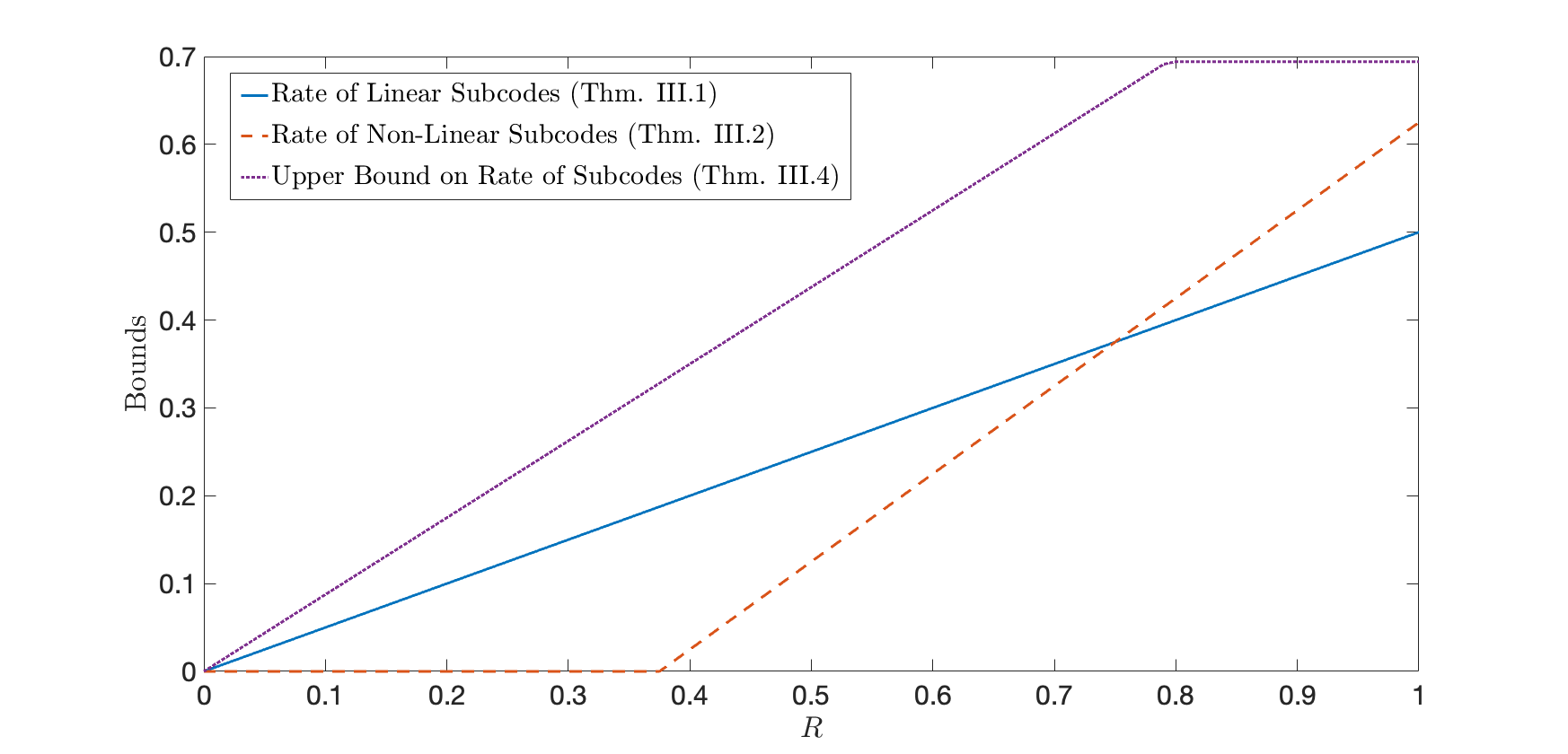
The proof of Theorem III.2 is provided in Section IV. Again, we note from the discussion in Section II-C, that Theorem III.2 implies that rates of at least $\max\left(0,C-\frac{3}{8}\right)$ are achievable over the $(d,\infty)$-RLL input-constrained BMS channel. Further, we observe that the lower bound in the theorem above beats the achievable rate of $\frac{R}{2}$ in Theorem III.1, when $R>0.75$.

Next, we state a theorem that provides upper bounds on the largest rate of linear $(d,\infty)$-RLL subcodes of RM codes, where the coordinates are ordered according to the lexicographic ordering. Fix any sequence of codes $\left\{{\hat{\mathcal{C}}_{m}}=\text{RM}(m,r_{m})\right\}_{m\geq 1}$ of rate $R\in(0,1)$ and let ${\overline{\mathsf{R}}^{(d)}(\hat{\mathcal{C}})}$ be the largest rate of linear $(d,\infty)$-RLL subcodes of $\left\{{\hat{\mathcal{C}}_{m}}\right\}_{m\geq 1}$. Formally,

where the maximization is over linear $(d,\infty)$-RLL subcodes ${\overline{\mathcal{H}}^{(d)}}$ of ${\hat{\mathcal{C}}_{m}}$. Then,

Thus, Theorem III.3 shows that the sequence of simple linear subcodes $\left\{{\mathcal{C}_{m}^{(d)}}\right\}_{m\geq 1}$, identified in Theorem III.1, is rate-optimal whenever $d+1$ is a power of $2$, in that it achieves the rate upper bound of $\frac{R}{d+1}$. Moreover, it follows from Theorem III.3, that the subcodes in Theorem III.2 must be non-linear when $R>0.75$. Theorem III.3 is proved in Section V-A. Also, from the discussion in Section II and from Theorem III.3, we see that the largest rate achievable over a $(d,\infty)$-RLL input-constrained BMS channel, using linear $(d,\infty)$-RLL subcodes of RM codes, when the sub-optimal bit-MAP or block-MAP decoders of the larger RM codes are used, is bounded above by $\frac{C}{d+1}$.

We remark here that the problem of identifying linear codes that are subsets of the set of $(d,\infty)$-RLL sequences of a fixed length, has been studied in [39]. The results therein show that the largest linear code within $S_{(d,\infty)}^{(m)}$ has rate no larger than $\frac{1}{d+1}$, as $m\to\infty$. However, such a result offers no insight into rates achievable over BMS channels.

Concluding the discussion on rates achievable using subcodes of RM codes, following the lexicographic coordinate ordering, we state a theorem that provides an upper bound on the largest rate of $(1,\infty)$-RLL subcodes of the sequence $\{{\mathcal{C}_{m}}=\text{RM}(m,r_{m})\}_{m\geq 1}$, where $r_{m}$ is as in (1). We formally define this largest rate to be

where the maximization is over $(1,\infty)$-RLL subcodes ${\mathcal{H}^{(1)}}$ of ${\mathcal{C}_{m}}$. Then,

The proof of the theorem is taken up in Section V-B. We note that the upper bound in the theorem above is an improvement over the upper bound in [37], due to the use of better upper bounds on the weight distribution, from [32], as compared to those in [40]. Figure 3 shows a comparison between the upper bound in Theorem III.4, and the lower bounds of Theorems III.1 and III.2, for the case when $d=1$. From the discussion in Section II-C, we see that Theorem III.4 shows that the rate achievable over $(1,\infty)$-RLL input-constrained BMS channels, using constrained subcodes of $\{{\mathcal{C}_{m}}\}_{m\geq 1}$, when the sub-optimal bit-MAP or block-MAP decoders of the larger RM codes are used, is bounded above by $\min\left(\frac{7C}{8},{\kappa_{1}}\right)$, where $C$ is the capacity of the unconstrained BMS channel. Figure 4 shows comparisons, for the specific case of the $(1,\infty)$-RLL input-constrained BEC, of the upper bound of $\min\left(\frac{7}{8}\cdot(1-\epsilon),{\kappa_{1}}\right)$, obtained by sub-optimal decoding, in Theorem III.4, with the achievable rate of ${\kappa_{1}}\cdot(1-\epsilon)$ (from [11] and [16]), and the numerically computed achievable rates using the Monte-Carlo method in [41] (or the stochastic approximation scheme in [15]). For large values of the erasure probability $\epsilon$, we observe that the upper bound of $\min\left(\frac{7}{8}\cdot(1-\epsilon),{\kappa_{1}}\right)$ lies below the achievable rates of [41], thereby indicating that it is not possible to achieve the capacity of the $(1,\infty)$-RLL input-constrained BEC, using $(1,\infty)$-RLL subcodes of $\{{\mathcal{C}_{m}}\}_{m\geq 1}$, when the bit-MAP or block-MAP decoders of $\{{\mathcal{C}_{m}}\}_{m\geq 1}$ are used for decoding. We conjecture that this numerically verified fact is indeed true.

Next, we consider situations where the coordinates of the RM codes follow orderings different from the standard lexicographic ordering. First, we study upper bounds on the rates of linear $(d,\infty)$-RLL subcodes of RM codes, whose coordinates are ordered according to a Gray ordering (see Section V-C for a description of a Gray ordering). For a fixed $R\in(0,1)$, let $\left\{{\mathcal{C}_{m}^{\text{G}}}\right\}_{m\geq 1}$ be any sequence of RM codes following a Gray coordinate ordering, such that rate$\left({\mathcal{C}_{m}^{\text{G}}}\right)\xrightarrow{m\to\infty}R$. Let ${\overline{\mathsf{R}}^{(d)}(\mathcal{C}^{\text{G}})}$ denote the largest rate of linear $(d,\infty)$-RLL subcodes of $\left\{{\mathcal{C}_{m}^{\text{G}}}\right\}_{m\geq 1}$. Formally,

where the maximization is over linear $(d,\infty)$-RLL subcodes ${\overline{\mathcal{H}}_{\text{G}}^{(d)}}$ of $\mathcal{C}_{m}^{\text{G}}(R)$. We obtain the following result:

The proof of Theorem III.5 is provided in Section V-C. Again, Theorem III.5 provides an upper bound on the rates achieved over a $(d,\infty)$-RLL input-constrained BMS channel, using linear subcodes of Gray-ordered RM codes of rate $R$, when the sub-optimal bit-MAP decoders of $\left\{{\mathcal{C}_{m}^{\text{G}}}\right\}_{m\geq 1}$ are used, for decoding.

Now, we consider arbitrary orderings of coordinates, defined by the sequence of permutations $\left(\pi_{m}\right)_{m\geq 1}$, with $\pi_{m}:[0:2^{m}-1]\to[0:2^{m}-1]$. As with the Gray coordinate ordering, we define the sequence of $\pi$-ordered RM codes $\left\{{\mathcal{C}_{m}^{\pi}}\right\}_{m\geq 1}$, with

where $\left\{{\hat{\mathcal{C}}_{m}}=\text{RM}(m,r_{m})\right\}_{m\geq 1}$ is any sequence of RM codes of rate $R$. We also define ${\overline{\mathcal{H}}_{\pi}^{(d)}}$ be the largest linear $(d,\infty)$-RLL subcode of ${\mathcal{C}_{m}^{\pi}}$. The theorem below is then shown to hold:

Section V-C contains the proof of Theorem III.6.

Finally, we design $(d,\infty)$-RLL constrained codes, whose rates improve on those in Theorems III.1 and III.2, by using a two-stage (or concatenated) encoding procedure that employs systematic RM codes of rate $R$.

It can be checked that the rates achieved using Theorem III.7 are better than those achieved using Theorem III.1 (and in fact, better than those achieved using any sequence of linear $(d,\infty)$-RLL subcodes of RM codes) and Theorem III.2, for low noise regimes of the BMS channel. For example, when $d=1$, the rates achieved using the codes in Theorem III.7 are better than those achieved using linear subcodes, for $R\gtrapprox 0.7613$, and are better than those achieved using the subcodes of Theorem III.2, for $R\lessapprox 0.55$ and $R\gtrapprox 0.79$. Figures 5 and 6 show comparisons between the lower bounds (achievable rates), under block-MAP decoding, in Theorems III.1, III.2, and III.7, with the coset-averaging bound of [24], for $d=1$ and $d=2$, respectively. While [24] provides existence results on rates achieved using cosets of RM codes, with the rates calculated therein being better than those in Theorem III.7 in the low noise regimes of the BMS channel, our construction is more explicit. The code construction leading to Theorem III.7, and the proof of achievability of the rate lower bound, is taken up in Section VI. We mention here that Theorem III.3 and Theorems III.5–III.7 first appeared in [42].

We end this section with a remark. Note that the all-ones codeword $\mathbf{1}$ belongs to the RM code. Since any codeword $\mathbf{c}$ that respects the $(0,1)$-RLL constraint can be written as $\mathbf{c}=\mathbf{1}+\mathbf{\hat{c}}$, where $\mathbf{\hat{c}}$ respects the $(1,\infty)$-RLL constraint, the lower and upper bounds of the theorems above hold for the rate of $(0,1)$-RLL subcodes as well. Moreover, since for any $k>1$, a $(0,1)$-RLL subcode of an RM code is a subset of a $(0,k)$-RLL subcode, the lower bounds of Theorems III.1, III.2, and III.7, hold over $(0,k)$-RLL input-constrained BMS channels as well.

References

- [1] B. H. Marcus, R. M. Roth, and P. H. Siegel, “An introduction to coding for constrained systems,” lecture notes. [Online]. Available: https://ronny.cswp.cs.technion.ac.il/wp-content/uploads/sites/54/2016/05/chapters1-9.pdf
- [2] K. A. S. Immink, P. H. Siegel, and J. K. Wolf, “Codes for digital recorders,” IEEE Transactions on Information Theory, vol. 44, no. 6, pp. 2260–2299, Oct. 1998.
- [3] K. A. S. Immink, “Runlength-limited sequences,” Proceedings of the IEEE, vol. 78, no. 11, pp. 1745–1759, 1990.
- [4] A. M. Fouladgar, O. Simeone, and E. Erkip, “Constrained codes for joint energy and information transfer,” IEEE Transactions on Communications, vol. 62, no. 6, pp. 2121–2131, 2014.
- [5] E. Arikan, “Channel polarization: A method for constructing capacity-achieving codes for symmetric binary-input memoryless channels,” IEEE Transactions on Information Theory, vol. 55, no. 7, pp. 3051–3073, 2009.
- [6] S. Kudekar, S. Kumar, M. Mondelli, H. D. Pfister, E. Şaşoǧlu, and R. L. Urbanke, “Reed-Muller codes achieve capacity on erasure channels,” IEEE Transactions on Information Theory, vol. 63, no. 7, pp. 4298–4316, 2017.
- [7] M. G. Luby, M. Mitzenmacher, M. A. Shokrollahi, and D. A. Spielman, “Efficient erasure correcting codes,” IEEE Transactions on Information Theory, vol. 47, no. 2, pp. 569–584, 2001.
- [8] T. J. Richardson, M. A. Shokrollahi, and R. L. Urbanke, “Design of capacity-approaching irregular low-density parity-check codes,” IEEE Transactions on Information Theory, vol. 47, no. 2, pp. 619–637, 2001.
- [9] S. Kudekar, T. Richardson, and R. L. Urbanke, “Spatially coupled ensembles universally achieve capacity under belief propagation,” IEEE Transactions on Information Theory, vol. 59, no. 12, pp. 7761–7813, 2013.
- [10] E. Zehavi and J. K. Wolf, “On runlength codes,” IEEE Transactions on Information Theory, vol. 34, no. 1, pp. 45–54, Jan. 1988.
- [11] Y. Li and G. Han, “Asymptotics of input-constrained erasure channel capacity,” IEEE Transactions on Information Theory, vol. 64, no. 1, pp. 148–162, Jan. 2018.
- [12] G. Han and B. Marcus, “Asymptotics of input-constrained binary symmetric channel capacity,” The Annals of Applied Probability, vol. 19, no. 3, pp. 1063–1091, 2009. [Online]. Available: https://doi.org/10.1214/08-AAP570
- [13] E. Ordentlich and T. Weissman, “Bounds on the entropy rate of binary hidden Markov processes,” in Entropy of Hidden Markov Processes and Connections to Dynamical Systems: Papers from the Banff International Research Station Workshop, B. Marcus, K. Petersen, and T. Weissman, Eds. London Mathematical Society Lecture Notes Series, Cambridge University Press, 2011, pp. 117–171.
- [14] O. Ordentlich, “Novel lower bounds on the entropy rate of binary hidden Markov processes,” in Proc. 2016 IEEE International Symposium on Information Theory (ISIT 2016), Barcelona, Spain, 10–15 July 2016, pp. 690–694.
- [15] V. A. Rameshwar and N. Kashyap, “Numerically computable lower bounds on the capacity of the -RLL input-constrained binary erasure channel,” in Proc. 2021 National Conference on Communications (NCC 2021), Kanpur, India, 27–30 July 2021.
- [16] V. A. Rameshwar and N. Kashyap, “Computable lower bounds for capacities of input-driven finite-state channels,” in Proc. 2020 IEEE International Symposium on Information Theory (ISIT 2020), virtual conference, 21–26 June 2020, pp. 2002–2007.
- [17] G. Reeves and H. D. Pfister, “Reed-Muller codes achieve capacity on BMS channels,” arXiv:2110.14631, Oct. 2021.
- [18] E. Abbe and C. Sandon, “A proof that Reed-Muller codes achieve Shannon capacity on symmetric channels,” arXiv e-prints, p. arXiv:2304.02509, Apr. 2023.
- [19] W. G. Bliss, “Circuitry for performing error correction calculations on baseband encoded data to eliminate error propagation,” IBM Technical Disclosure Bulletin, vol. 23, pp. 4633–4634, 1981. [Online]. Available: https://cir.nii.ac.jp/crid/1570009751553045248
- [20] M. Mansuripur, “Enumerative modulation coding with arbitrary constraints and postmodulation error correction coding for data storage systems,” in Optical Data Storage ’91, J. J. Burke, T. A. Shull, and N. Imamura, Eds. Society of Photo-Optical Instrumentation Engineers (SPIE) Conference Series, 1991, vol. 1499, pp. 72–86.
- [21] K. Immink, “A practical method for approaching the channel capacity of constrained channels,” IEEE Transactions on Information Theory, vol. 43, no. 5, pp. 1389–1399, 1997.
- [22] J. Fan and A. Calderbank, “A modified concatenated coding scheme, with applications to magnetic data storage,” IEEE Transactions on Information Theory, vol. 44, no. 4, pp. 1565–1574, 1998.
- [23] J. Campello de Souza, B. Marcus, R. New, and B. Wilson, “Constrained systems with unconstrained positions,” IEEE Transactions on Information Theory, vol. 48, no. 4, pp. 866–879, 2002.
- [24] A. Patapoutian and P. Kumar, “The subcode of a linear block code,” IEEE Transactions on Information Theory, vol. 38, no. 4, pp. 1375–1382, 1992.
- [25] I. Tal, H. D. Pfister, A. Fazeli, and A. Vardy, “Polar codes for the deletion channel: weak and strong polarization,” IEEE Transactions on Information Theory, vol. 68, no. 4, pp. 2239–2265, 2022.
- [26] E. Şaşoǧlu and I. Tal, “Polar coding for processes with memory,” IEEE Transactions on Information Theory, vol. 65, no. 4, pp. 1994–2003, 2019.
- [27] Y. Li and V. Y. F. Tan, “On the capacity of channels with deletions and states,” IEEE Transactions on Information Theory, vol. 67, no. 5, pp. 2663–2679, 2021.
- [28] E. Abbe, A. Shpilka, and M. Ye, “Reed-Muller codes: Theory and algorithms,” IEEE Transactions on Information Theory, vol. 67, no. 6, pp. 3251–3277, 2021.
- [29] E. Abbe, A. Shpilka, and A. Wigderson, “Reed-Muller codes for random erasures and errors,” IEEE Transactions on Information Theory, vol. 61, no. 10, pp. 5229–5252, 2015.
- [30] T. Kaufman, S. Lovett, and E. Porat, “Weight distribution and list-decoding size of Reed-Muller codes,” IEEE Transactions on Information Theory, vol. 58, no. 5, pp. 2689–2696, 2012.
- [31] O. Sberlo and A. Shpilka, “On the performance of Reed-Muller codes with respect to random errors and erasures,” in Proc. 31st Annual ACM-SIAM Symposium on Discrete Algorithms (SODA’20), Salt Lake City, Utah, USA, 2020, pp. 1357–1376.
- [32] A. Rao and O. Sprumont, “On list decoding transitive codes from random errors,” 2022. [Online]. Available: https://homes.cs.washington.edu/˜anuprao/pubs/rmlist.pdf
- [33] R. Roth, Introduction to Coding Theory. Cambridge University Press, 2006.
- [34] T. M. Cover and J. A. Thomas, Elements of Information Theory, 2nd ed. Wiley-India, 2010.
- [35] R. G. Gallager, Information Theory and Reliable Communication. Wiley, 1968.
- [36] F. MacWilliams and N. Sloane, The Theory of Error-Correcting Codes, 2nd ed. North-Holland, 1978.
- [37] V. A. Rameshwar and N. Kashyap, “On the performance of Reed-Muller codes over -RLL input-constrained BMS channels,” in Proc. 2022 IEEE International Symposium on Information Theory (ISIT 2022), Espoo, Finland, June 26 – July 1 2022, pp. 1755–1760.
- [38] J. K. Wolf, “Invited talk on the magnetic recording channel,” 26th Annual Allerton Conference, Sep. 1988.
- [39] G. Lechner, I. Land, and A. Grant, “Linear and non-linear run length limited codes,” IEEE Communications Letters, vol. 19, no. 7, pp. 1085–1088, Jul. 2015.
- [40] A. Samorodnitsky, “An upper bound on norms of noisy functions,” IEEE Transactions on Information Theory, vol. 66, no. 2, pp. 742–748, 2020.
- [41] D. Arnold, H.-A. Loeliger, P. Vontobel, A. Kavcic, and W. Zeng, “Simulation-based computation of information rates for channels with memory,” IEEE Transactions on Information Theory, vol. 52, no. 8, pp. 3498–3508, 2006.
- [42] V. A. Rameshwar and N. Kashyap, “Linear runlength-limited subcodes of Reed-Muller codes and coding schemes for input-constrained BMS channels,” arXiv:2205.04153, 2022.
- [43] W. C. Huffman and V. Pless, Fundamentals of Error-Correcting Codes. Cambridge University Press, 2003.
- [44] R. Diestel, Graph Theory, 5th ed. Springer, 2017.
- [45] S. Kudekar, S. Kumar, M. Mondelli, H. D. Pfister, and R. Urbanke, “Comparing the bit-MAP and block-MAP decoding thresholds of Reed-Muller codes on BMS channels,” in Proc. 2016 IEEE International Symposium on Information Theory (ISIT 2016), Barcelona, Spain, 10–15 July 2016, pp. 1755–1759.
- [46] R. Adler, D. Coppersmith, and M. Hassner, “Algorithms for sliding block codes – an application of symbolic dynamics to information theory,” IEEE Transactions on Information Theory, vol. 29, no. 1, pp. 5–22, 1983.
- [47] R. Durrett, Probability: Theory and Examples, 5th ed. Cambridge University Press, 2019.