跳到论文正文
W Papers独立论文阅读器 arXiv:2211.04919 论文正文 计算阅读时间 · 0%
引用这篇论文根据当前论文元数据生成,正式投稿前建议核对。


License: CC BY 4.0
arXiv:2211.04919v1 [math.DS] 09 Nov 2022

Thermodynamic formalism for general iterated function systems with measures

Jader E. Brasil Affiliation:  jaderebrasil@gmail.com    Elismar R. Oliveira    Rafael Rigão Souza
August 11, 2026
Abstract

This paper introduces a theory of Thermodynamic Formalism for Iterated Function Systems with Measures (IFSm). We study the spectral properties of the Transfer and Markov operators associated to a IFSm. We introduce variational formulations for the topological entropy of holonomic measures and the topological pressure of IFSm given by a potential. A definition of equilibrium state is then natural and we prove its existence for any continuous potential. We show, in this setting, a uniqueness result for the equilibrium state requiring only the Gâteaux differentiability of the pressure functional.

MSC2010: 37D35, 37B40, 28Dxx.
Keywords: Iterated Function System, Thermodynamic Formalism, Ergodic Theory, Transfer Operator, Entropy, Pressure, Equilibrium States.

1 Introduction

The modern study of Iterated Function Systems (IFS for short) come back to the early 80’s with the works of J. Hutchinson [20] and M. Barnsley [3]. In these papers, the theory was unified both in the geometric and the analytical point of view, generating what we call today the Hutchinson-Barnsley theory for IFS. An IFS is a family of maps acting from a set to itself. Under good contraction hypothesis there exist an invariant compact set called the fractal attractor. Moreover, if we add weights having good continuity hypothesis, the IFS acts on probabilities having an invariant probability whose support is the fractal attractor set. We observe that several works on geometric features of fractals were done in the previous decades by Mandelbrot and others, but after the 80’s the IFS assumed the central role in the generation and study of fractals and its applications.

For a dynamical system given by a map T:X→XT:X\to X, an initial point x0∈Xx_{0}\in X is iterated by TT producing the orbit {x0,T⁡(x0),T2​(x0),…}\{x_{0},T(x_{0}),T^{2}(x_{0}),...\}, whose limit or the cluster points are the objects of main interest, from a dynamical point of view. On the other hand, for an IFS (X,τθ)θ∈Θ(X,\tau_{\theta})_{\theta\in\Theta}, we iterate the initial point by choosing at each step a possibly different map τθ:X→X\tau_{\theta}:X\to X, indexed by the generally finite set Θ\Theta, producing multiple orbits {Zj,j≥0}={Z0=x0,Z1=τθ0​(x0),Z2=τθ1​(τθ0​(x0)),…}\{Z_{j},j\geq 0\}=\{Z_{0}=x_{0},Z_{1}=\tau_{\theta_{0}}(x_{0}),Z_{2}=\tau_{\theta_{1}}(\tau_{\theta_{0}}(x_{0})),...\}. We notice that the orbit is now a set of orbits controlled by the sequence (θ0,θ1,…)∈Θℕ(\theta_{0},\theta_{1},...)\in\Theta^{\mathbb{N}}. To avoid this complication Hutchinson defined the fractal operator F:K⁡(X)→K⁡(X)F:K(X)\to K(X) by

F⁡(B)=⋃θ∈Θτθ​(B),F(B)=\bigcup_{\theta\in\Theta}\tau_{\theta}(B),

for B∈K⁡(X)B\in K(X), where K⁡(X)K(X) is the family of nonempty compact sets of XX. This operator is called the Hutchinson-Barnsley operator and a compact set is invariant or fractal if F⁡(Ω)=ΩF(\Omega)=\Omega. Additionally Ω\Omega is a fractal attractor if the orbit of BB by FF, given by {B,F⁡(B),F2​(B),…}\{B,F(B),F^{2}(B),...\} converge, w.r.t. the Hausdorff-Pompeiu metric to Ω\Omega, for any B∈K⁡(X)B\in K(X) (see [5] for details on the Hausdorff-Pompeiu metric).

Other possible point of view to understand the dynamics of an IFS is the probabilistic one. Suppose XX is now a metric space and let 𝒫⁡(X)\mathcal{P}(X) be the set of Borel probability measures defined on XX. In this case we consider that, in each step the function to be iterated is chosen according to some probability, which produces a stochastic process {X0,X1,X2,…}\{X_{0},X_{1},X_{2},...\} where each Xj+1∈XX_{j+1}\in X is randomly chosen according to a distribution which is obtained from the previous XjX_{j} by a transition kernel using the IFS law. To illustrate that, we consider the classical case of IFS with constant probabilities studied by Hutchinson, Barnsley and many others in the beginnings of the 80’s: we consider Θ={1,2,…,n}\Theta=\{1,2,...,n\}, meaning that we have a finite number of maps, and each one is chosen according to a probability pj>0p_{j}>0 where p1+⋯+pn=1p_{1}+\cdots+p_{n}=1, constituting an IFS with probabilities (IFSp for short). We denote by C⁡(X,ℝ)C(X,\mathbb{R}) the Banach space of all real continuous functions equipped with supremum norm ∥∥∞\|\;\|_{\infty}. Under this conditions the classic transfer operator (also called Ruelle operator, see Ruelle [29, 30], Walters [33] and Fan [14]) is given by

Bq​(f)​(x)=∫Θf⁡(τθ​(x))​d​qx​(θ)=∑j=1npj​f​(τj​(x)),B_{q}(f)(x)=\int_{\Theta}f(\tau_{\theta}(x))dq_{x}(\theta)=\sum_{j=1}^{n}p_{j}\,f(\tau_{j}(x)), (1)

for any f∈C⁡(X,ℝ)f\in C(X,\mathbb{R}), where the measure qxq_{x} is given by d​qx​(θ)=∑j=1npj​δj​(θ),∀x∈Xdq_{x}(\theta)=\sum_{j=1}^{n}p_{j}\delta_{j}(\theta),\;\forall x\in X. The dual of BqB_{q} is a Markov operator (see [11], [22] and[3], for details on Markov operators and its connection with IFS) acting on μ\mu. The operator ℒq​(μ):=Bq∗​(μ)\mathcal{L}_{q}(\mu):=B_{q}^{*}(\mu), is implicitly defined by the property

∫Xf​d​ℒq​(μ)=∫XBq​(f)​(x)​𝑑μ,\int_{X}fd\mathcal{L}_{q}(\mu)=\int_{X}B_{q}(f)(x)d\mu, (2)

for any f∈C⁡(X,ℝ)f\in C(X,\mathbb{R}). Given an initial distribution μ0\mu_{0}, we iterate it by the Markov operator M:𝒫⁡(X)→𝒫⁡(X)M:\mathcal{P}(X)\to\mathcal{P}(X) obtaining the distributions μ0,μ1=ℒq​(μ0),μ2=ℒq2​(μ0),…∈𝒫⁡(X)\mu_{0},\mu_{1}=\mathcal{L}_{q}(\mu_{0}),\mu_{2}=\mathcal{L}_{q}^{2}(\mu_{0}),...\in\mathcal{P}(X). We have Xn∼μnX_{n}\sim\mu_{n} for all n≥0n\geq 0. Analogously to the fractal attractor, we say that μ∈𝒫⁡(X)\mu\in\mathcal{P}(X) is an invariant measure if ℒq​(μ)=μ\mathcal{L}_{q}(\mu)=\mu and that μ∈𝒫⁡(X)\mu\in\mathcal{P}(X) is an attracting invariant measure (or Hutchinson-Barnsley measure) if ℒqj​(μ0)\mathcal{L}_{q}^{j}(\mu_{0}) converge to μ\mu w.r.t. the Monge-Kantorovich metric(see [20]), for any μ0∈𝒫⁡(X)\mu_{0}\in\mathcal{P}(X). It is possible to prove that the support of the invariant attracting measure is the fractal attractor (see [20]).

The final feature of an IFS dynamics we need to understand is the connections between IFS orbits and invariant measures. The first connection is given by a celebrated result due to M. Barnsley, known as the Chaos Game Theorem (CGT for short), which claims that, from the initial probabilities pjp_{j}’s, we can build a probability ℙ\mathbb{P} over the space Θℕ\Theta^{\mathbb{N}} such that for ℙ\mathbb{P}-a.e. (θ0,θ1,…)⊂Θℕ(\theta_{0},\theta_{1},...)\subset\Theta^{\mathbb{N}} the corresponding orbit {x0,τθ0​(x0),τθ1​(τθ0​(x0)),…}\{x_{0},\tau_{\theta_{0}}(x_{0}),\tau_{\theta_{1}}(\tau_{\theta_{0}}(x_{0})),...\} approximate the fractal attractor Ω\Omega, for any initial point x0x_{0}. The second connection is given by the Elton’s Ergodic Theorem (EET for short) [13] claiming that, from the initial probabilities pjp_{j}’s, we can build a probability ℙ\mathbb{P} over the space Θℕ\Theta^{\mathbb{N}} such that ℙ\mathbb{P}-a.e. (θ0,θ1,…)⊂Θℕ(\theta_{0},\theta_{1},...)\subset\Theta^{\mathbb{N}}, the corresponding asymptotic average of visits of the orbit {x0,τθ0​(x0),τθ1​(τθ0​(x0)),…}\{x_{0},\tau_{\theta_{0}}(x_{0}),\tau_{\theta_{1}}(\tau_{\theta_{0}}(x_{0})),...\} to a measurable set B⊂XB\subset X is equal to μ⁡(B)\mu(B), if μ⁡(∂(B))=0\mu(\partial(B))=0, analogously to the usual Birkhoff ergodic theorem for a single map, where μ\mu is the invariant measure of the IFS in consideration. For continuous functions it means that

1N(f(x0)+f(τθ0(x0))+⋯+f(τθN−1(⋯τθ0(x0))))→∫Xfdμ,\frac{1}{N}\left(f(x_{0})+f(\tau_{\theta_{0}}(x_{0}))+\cdots+f(\tau_{\theta_{N-1}}(\cdots\tau_{\theta_{0}}(x_{0})))\right)\to\int_{X}fd\mu,

for any f∈C⁡(X,ℝ)f\in C(X,\mathbb{R}), as N→∞N\to\infty. In other words

1N(δx0+δτθ0​(x0)+⋯+δτθN−1(⋯τθ0(x0)))→μ,\frac{1}{N}\left(\delta_{x_{0}}+\delta_{\tau_{\theta_{0}}(x_{0})}+\cdots+\delta_{\tau_{\theta_{N-1}}(\cdots\tau_{\theta_{0}}(x_{0}))}\right)\to\mu,

in distribution. In synthesis, the CGT and the EET are random procedures to approximate the fractal attractor and the invariant measure, respectively.

The study of the conditions under which we have, for a given IFS, a fractal attractor which is the support of an invariant measure is called the Hutchinson-Barnsley theory. Such conditions have been extremely relaxed and generalized in several ways in the past forty years. A first generalization, yet for Θ={1,2,…,n}\Theta=\{1,2,...,n\}, was for IFSp where the constant probabilities pj>0p_{j}>0 such that p1+⋯+pn=1p_{1}+\cdots+p_{n}=1 were replaced by variable probabilities pj​(x)>0p_{j}(x)>0 where p1​(x)+⋯+pn​(x)=1p_{1}(x)+\cdots+p_{n}(x)=1 for all x∈Xx\in X. Now, the transfer operator is defined by

Bq​(f)​(x)=∫Θf⁡(τθ​(x))​d​qx​(θ)=∑j=1npj​(x)​f​(τj​(x)),B_{q}(f)(x)=\int_{\Theta}f(\tau_{\theta}(x))dq_{x}(\theta)=\sum_{j=1}^{n}p_{j}(x)\,f(\tau_{j}(x)), (3)

where the measure qxq_{x} is given by d​qx​(θ)=∑j=1npj​(x)​δj​(θ),∀x∈Xdq_{x}(\theta)=\sum_{j=1}^{n}p_{j}(x)\delta_{j}(\theta),\;\forall x\in X, for any f∈C⁡(X,ℝ)f\in C(X,\mathbb{R}), Very general conditions for the existence of the invariant measure for such IFS are given in [4]. We point out that the EET was also proved for variable probabilities and finite functions in [13].

In Fan [14], 1999, the condition p1​(x)+⋯+pn​(x)=1p_{1}(x)+\cdots+p_{n}(x)=1 is finally dropped assuming only that each pθ​(x)≥0p_{\theta}(x)\geq 0 for θ∈{1,…,n}\theta\in\{1,...,n\}. In this work Fan study a contractive system which is a triplet (X,τθ,pθ)θ∈{1,…,n}(X,\tau_{\theta},p_{\theta})_{\theta\in\{1,...,n\}}, where each τθ\tau_{\theta} is a contractive map and each pθ​(x)≥0p_{\theta}(x)\geq 0 for θ=1,…,n\theta=1,...,n, generalizing the notion of IFS with probabilities. In this setting, Fan proves a Ruelle-Perron-Frobenius theorem (RPF theorem, for short), meaning the existence of a positive eigenfunction for the operator BqB_{q} and an eigenmeasure for the dual operator Bq∗B_{q}^{*} with the same eigenvalue which is the spectral radius of BqB_{q}.

The next key improvement was given by Stenflo [32], where random iterations are used to represent the iterations of a so called IFS with probabilities, (X,τθ,μ)θ∈Θ(X,\tau_{\theta},\mu)_{\theta\in\Theta} for an arbitrary measurable space Θ\Theta. The approach here is slightly different from the previous works on IFS with probabilities, instead considering weights, the iterations from Z0∈XZ_{0}\in X are Zj+1=τIj​(Zj)Z_{j+1}=\tau_{I_{j}}(Z_{j}) governed by a sequence of i.i.d variables {Ij∈Θ}j∈ℕ\{I_{j}\in\Theta\}_{j\in\mathbb{N}}, with distribution μ\mu, generating a Markov chain {Zj,j≥0}\{Z_{j},\;j\geq 0\} with transfer operator given by

Bq​(f)​(x)=∫Θf⁡(τθ​(x))​d​qx​(θ)=∑j=1npj​(x)​f​(τj​(x)),B_{q}(f)(x)=\int_{\Theta}f(\tau_{\theta}(x))dq_{x}(\theta)=\sum_{j=1}^{n}p_{j}(x)\,f(\tau_{j}(x)), (4)

where the measure qxq_{x} is given by d​qx​(θ)=d​μ​(θ),∀x∈Xdq_{x}(\theta)=d\mu(\theta),\;\forall x\in X, the for any f∈C⁡(X,ℝ)f\in C(X,\mathbb{R}), The main goal of Stenflo [32] is to establish, when BqB_{q} is Feller, the existence of an unique attracting invariant measure π\pi, for this Markov chain.

The approach in our paper is a generalization of Stenflo [32], (4), and all classical settings (1) and (3). We take a family qx​(⋅)∈ℳ​(Θ)q_{x}(\cdot)\in\mathcal{M}(\Theta), indexed by x∈Xx\in X, generating a Markov chain with transfer operator given by

Bq​(f)​(x)=∫Θf⁡(τθ​(x))​d​qx​(θ),B_{q}(f)(x)=\int_{\Theta}f(\tau_{\theta}(x))dq_{x}(\theta),

for any f∈C⁡(X,ℝ)f\in C(X,\mathbb{R}). The meaning of the distribution qx​(⋅)∈ℳ​(Θ)q_{x}(\cdot)\in\mathcal{M}(\Theta) is such that, the position xx of a previous iteration of the IFS determine the distribution qx​(⋅)q_{x}(\cdot) of θ\theta used to choose the function τθ\tau_{\theta} and produce the new point τθ​(x)\tau_{\theta}(x). When qx=μq_{x}=\mu, for any x∈Xx\in X, is a constant distribution we recover the setting from Stenflo [32].

In our setting the IFSm (X,τθ,q)θ∈Θ(X,\tau_{\theta},q)_{\theta\in\Theta} can be studied as the sample paths of the Markov process {Zj,j≥0}\{Z_{j},\;j\geq 0\} with initial distribution μ0=μ∈ℳ⁡(X)\mu_{0}=\mu\in\mathcal{M}(X) and μj+1=ℒq​(μj)\mu_{j+1}=\mathcal{L}_{q}(\mu_{j}), where for any ν∈ℳ⁡(X)\nu\in\mathcal{M}(X),

∫Xf⁡(x)​d​ℒq​(ν)​(x)=∫XBq​(f)​(x)​𝑑ν​(x),\int_{X}f(x)d\mathcal{L}_{q}(\nu)(x)=\int_{X}B_{q}(f)(x)d\nu(x),

for any f∈C⁡(X,ℝ)f\in C(X,\mathbb{R}). Such degree of generality is necessary to enlarge the range of application for the IFS theory, specially the thermodynamic formalism. In Section 7 we present a situation where we believe the tools developed in the previous sections can be applied when analyzing an interesting problem in economics.

Our goal is to present a complete theory of thermodynamical formalism for these IFS with measures, that is, good definitions for transfer operators, invariant measures, entropy, pressure, equilibrium measures and a variational principle. Finally, we want to use these tools to characterize the solutions of the ergodic optimization problem.

For sake of completeness we would like to point out that we do not prove a RPF theorem for those systems, only the existence of positive eigenfunctions, but we establish all the results that can be derived if we have assumed such a property. To the best of our knowledge the RPF theorem for IFSm has not been established an it is a very hard problem. There are several works on the matter of finding IFS for which the RPF theorem holds. Those IFS are said to have the RPF property. In 2009 Lopes and Oliveira [24] studied those systems renaming it as weighted systems or IFS with weights, having the RPF property, producing a self contained notion of entropy and topological pressure through a variational principle for holonomic measures allowing to establish a thermodynamical formalism for IFS. Other approaches for IFS thermodynamic formalism were developed by Urbański [31, 25, 18] and many others.

It’s worth to mention that, in Urbański et al. [18] a thermodynamic formalism for conformal infinite (countable) iterated function systems is presented using the conformal structure via partition functions. Also in Käenmäki [21] a thermodynamical formalism for IFS is studied with the help of cylinder functions, where general IFS means that (X,τθ)θ∈Θ(X,\tau_{\theta})_{\theta\in\Theta} and Θ\Theta is the increasing union of finite alphabets. In Lopes et al. [23] a thermodynamic formalism for shift spaces, taking values on a compact metric space is presented, although this problem is closely related to thermodynamic formalism for IFS when we associate the pre images of the shift map with a respective maps producing an infinite IFS. Also in [1] a variational principle for the specific entropy on the context of symbolic dynamics of compact metric space alphabets was developed generalizing somehow the results in [24].

In our work we will extend the variational results in Lopes and Oliveira [24] and, more recently, the preprint Cioletti and Oliveira [8], to a general IFS called IFS with measures (IFSm), (X,τθ,q)θ∈Θ(X,\tau_{\theta},q)_{\theta\in\Theta} for an arbitrary compact space Θ\Theta (see Dumitru [12] for the Hutchinson-Barnsley theory for such infinite systems or Lukawska [17] for infinite countable ones. Other related articles are [15, 19, 27, 28, 26, 7]). We point out that we do not use partitions to construct our entropy, only an integral formulation, and the variational principle is taken over the holonomic measures which enclose the invariant ones.

The structure of the paper is the following: in Section 2, we present the basic definitions on IFS with measures (IFSm) and a fundamental result about the eigenspace associated to the maximal eigenvalue of the transfer operator. We also prove the existence of a positive eigenfunction for the transfer operator associated to the spectral radius and give a constructive proof of the existence of equilibrium states. In Section 3 we define the Markov operator, which in the case of a normalized IFSm gives the evolution of the distribution of the associated Markov process, and show that the set of eigenmeasures for it is non-empty. In Section 4, we introduce holonomic measures, which play the role of invariant measures in the IFS setting. In Section 5 we define entropy for a IFSm, the topological pressure of a given potential function, as well as the concept of equilibrium states. In a remark in the end of this section we show how the classical thermodynamical formalism for a dynamical system is a particular case of the IFSm Thermodynamic Formalism. In Section 6 a uniqueness result for the equilibrium states is obtained. Finally, in Section 7 we present a possible application in economic theory of the theory developed in the previous sections.

2 IFSm and Transfer Operator

In this section we set up the basic notation and present a fundamental result about the eigenspace associated to the maximal eigenvalue (or spectral radius) of the transfer operator.

In this paper X,Θ\textbf{X},\Theta are compact metric spaces, equipped with ℬ⁡(X)\mathscr{B}(\textbf{X}) and ℬ⁡(Θ)\mathscr{B}(\Theta) respectively the Borel σ\sigma-algebra for X and Θ\Theta.

The Banach space of all real continuous functions equipped with supremum norm is denoted by C⁡(X,ℝ)C(\textbf{X},\mathbb{R}). Its topological dual, as usual, is identified with ℳs​(X)\mathscr{M}_{s}(\textbf{X}), the space of all finite Borel signed measures endowed with total variation norm. We use the notation ℳ1​(X)\mathscr{M}_{1}(X) for the set of all Borel probability measures over XX supplied with the weak-∗* topology. Since we are assuming that XX is a compact metric space then we have that the topological space ℳ1​(X)\mathscr{M}_{1}(X) is compact and metrizable.

Take q=(qx)x∈X\text{q}\hskip 0.50003pt={(\text{q}\hskip 0.50003pt_{x})}_{x\in\textbf{X}} a collection of measures on ℬ⁡(Θ)\mathscr{B}(\Theta), such that

  1. (q1)

    supq≡supx∈Xqx​(Θ)<∞\displaystyle\sup\text{q}\hskip 0.50003pt\equiv\sup_{x\in X}\text{q}\hskip 0.50003pt_{x}(\Theta)<\infty,

  2. (q2)

    infq≡infx∈Xqx​(Θ)>0\displaystyle\inf\text{q}\hskip 0.50003pt\equiv\inf_{x\in\textbf{X}}\text{q}\hskip 0.50003pt_{x}(\Theta)>0,

  3. (q3)

    x↦qx​(A)\displaystyle x\mapsto\text{q}\hskip 0.50003pt_{x}(A) is a Borel map, i.e, is ℬ⁡(X)\mathscr{B}(\textbf{X})-measurable for all fixed A∈ℬ⁡(Θ)A\in\mathscr{B}(\Theta),

  4. (q4)

    x↦qx\displaystyle x\mapsto\text{q}\hskip 0.50003pt_{x} is weak∗-continuous.

An Iterated Function System with measures qq, IFSm for short, is a triple ℛq=(X,τ,q)\mathcal{R}_{\text{q}\hskip 0.40974pt}=(\textbf{X},\tau,\text{q}\hskip 0.50003pt), where τ=(τθ)θ∈Θ\tau={(\tau_{\theta})}_{\theta\in\Theta} is a collection of functions from X to itself with the following property

  1. (τ\tau1)

    τ:(Θ,X)↦X\tau:(\Theta,\textbf{X})\mapsto\textbf{X}, where τ⁡(θ,x)=τθ​(x)\tau(\theta,x)=\tau_{\theta}(x) is continuous.

The ℛq\mathcal{R}_{\text{q}\hskip 0.40974pt} is said to be normalized if for all x∈Xx\in\textbf{X}, qx\text{q}\hskip 0.50003pt_{x} is a probability measure.

Definition 2.1.

Let ℛq=(X,τ,q)\mathcal{R}_{\text{q}\hskip 0.40974pt}=(\textbf{X},\tau,\text{q}\hskip 0.50003pt) be an IFSm. The Transfer Operator Bq:C⁡(X,ℝ)⮌\text{B}\hskip 0.50003pt_{\text{q}\hskip 0.40974pt}:C(\textbf{X},\mathbb{R})\righttoleftarrow associated to ℛq\mathcal{R}_{\text{q}\hskip 0.40974pt} is defined by:

Bq​(f)​(x)=∫Θf⁡(τθ​(x))​dqx​(θ),∀x∈X.\text{B}\hskip 0.50003pt_{\text{q}\hskip 0.40974pt}(f)(x)=\int_{\Theta}f(\tau_{\theta}(x))\,\text{d}\text{q}\hskip 0.50003pt_{x}(\theta),\qquad\forall x\in X.

Bq\text{B}\hskip 0.50003pt_{\text{q}\hskip 0.40974pt} is well defined. In fact, Bq\text{B}\hskip 0.50003pt_{\text{q}\hskip 0.40974pt} is continuous once that

‖Bq​(f)‖∞=supx|∫f⁡(τθ​(x))​dqx​(θ)|≤supq​‖f‖∞<∞.\left\lVert\text{B}\hskip 0.50003pt_{\text{q}\hskip 0.40974pt}(f)\right\rVert_{\infty}=\sup_{x}\left\lvert\int\,f(\tau_{\theta}(x))\,\text{d}\text{q}\hskip 0.50003pt_{x}(\theta)\right\rvert\leq\sup\text{q}\hskip 0.50003pt\left\lVert f\right\rVert_{\infty}<\infty.

Futhermore, for a fixed f∈C⁡(X,ℝ)f\in C(\textbf{X},\mathbb{R}) and x∈Xx\in\textbf{X}, given ε>0\varepsilon>0, take δ>0\delta>0 s.t.

supθ∈Θd⁡(f⁡(τθ​(x)),f⁡(τθ​(y)))<ε2​supq,\sup_{\theta\in\Theta}d(f(\tau_{\theta}(x)),f(\tau_{\theta}(y)))<\frac{\varepsilon}{2\sup\text{q}\hskip 0.50003pt},

and

|∫Θf⁡(τθ​(x))​d​qx​(θ)−∫Θf⁡(τθ​(x))​d​qy​(θ)|<ε2,\left\lvert\int_{\Theta}f(\tau_{\theta}(x))d\text{q}\hskip 0.50003pt_{x}(\theta)-\int_{\Theta}f(\tau_{\theta}(x))d\text{q}\hskip 0.50003pt_{y}(\theta)\right\rvert<\frac{\varepsilon}{2},

for all y∈Xy\in\textbf{X} with d⁡(x,y)<δd(x,y)<\delta. Then,

|\displaystyle| Bq​(f)​(x)−Bq​(f)​(y)|=|∫Θf⁡(τθ​(x))​dqx​(θ)−∫Θf⁡(τθ​(y))​dqy​(θ)|\displaystyle\text{B}\hskip 0.50003pt_{\text{q}\hskip 0.40974pt}(f)(x)-\text{B}\hskip 0.50003pt_{\text{q}\hskip 0.40974pt}(f)(y)|=\left\lvert\int_{\Theta\hskip-6.02249pt}f(\tau_{\theta}(x))\,\text{d}\text{q}\hskip 0.50003pt_{x}(\theta)-\int_{\Theta\hskip-6.02249pt}f(\tau_{\theta}(y))\,\text{d}\text{q}\hskip 0.50003pt_{y}(\theta)\right\rvert
≤∫Θ|f⁡(τθ​(x))−f⁡(τθ​(y))|​dqx​(θ)+|∫Θf⁡(τθ​(y))​dqx​(θ)−∫Θf⁡(τθ​(y))​dqy​(θ)|\displaystyle\leq\int_{\Theta\hskip-6.02249pt}\left\lvert f(\tau_{\theta}(x))-f(\tau_{\theta}(y))\right\rvert\,\text{d}\text{q}\hskip 0.50003pt_{x}(\theta)+\left\lvert\int_{\Theta\hskip-6.02249pt}f(\tau_{\theta}(y))\,\text{d}\text{q}\hskip 0.50003pt_{x}(\theta)-\int_{\Theta\hskip-6.02249pt}f(\tau_{\theta}(y))\,\text{d}\text{q}\hskip 0.50003pt_{y}(\theta)\right\rvert
<ε2​supq​∫Θdqx​(θ)+ε2=ε2+ε2=ε.\displaystyle<\frac{\varepsilon}{2\sup\text{q}\hskip 0.50003pt}\int_{\Theta}\,\text{d}\text{q}\hskip 0.50003pt_{x}(\theta)+\frac{\varepsilon}{2}=\frac{\varepsilon}{2}+\frac{\varepsilon}{2}=\varepsilon.

This shows that, for f∈C⁡(X,ℝ)f\in C(\textbf{X},\mathbb{R}) and x∈Xx\in\textbf{X}, given ε>0\varepsilon>0, there is δ>0\delta>0 such that for every d⁡(x,y)<δd(x,y)<\delta, |Bq​(f)​(x)−Bq​(f)​(y)|<ϵ\left\lvert\text{B}\hskip 0.50003pt_{\text{q}\hskip 0.40974pt}(f)(x)-\text{B}\hskip 0.50003pt_{\text{q}\hskip 0.40974pt}(f)(y)\right\rvert<\epsilon, therefore Bq​(f)​(x)\text{B}\hskip 0.50003pt_{\text{q}\hskip 0.40974pt}(f)(x) is continuous.

When dealing with the spectral radius of a positive operator, via Gelfand’s formula, we will need to consider the norm of iterates of such operator, which is defined by a supremum which is attained in the constant function, as we will see in the proof of Theorem 2.5. For this reason we will need the following proposition:

Proposition 2.2.

Let ℛq=(X,τ,q)\mathcal{R}_{\text{q}\hskip 0.40974pt}=(\textbf{X},\tau,\text{q}\hskip 0.50003pt) be a IFSm. Then for the NN-th iteration of Bq\text{B}\hskip 0.50003pt_{\text{q}\hskip 0.40974pt} we have

BqN​(1)​(x)=∫ΘNdPxq​(θ0,…,θN−1)\text{B}\hskip 0.50003pt_{\text{q}\hskip 0.40974pt}^{N}(1)(x)=\int_{\Theta^{N}}\,\text{dP}_{x}^{\hskip 0.85355pt\text{q}\hskip 0.40974pt}\hskip 0.09995pt(\theta_{0},\ldots,\theta_{N-1})

where,

dPxq​(θ0,…,θN−1)≡∏j=1NdqxN−j​(θN−j)\displaystyle\,\text{dP}_{x}^{\hskip 0.85355pt\text{q}\hskip 0.40974pt}\hskip 0.09995pt(\theta_{0},\ldots,\theta_{N-1})\equiv\prod_{j=1}^{N}\,\text{d}\text{q}\hskip 0.50003pt_{x_{N-j}}(\theta_{N-j}), x0=xx_{0}=x and xj+1=τθj​xjx_{j+1}=\tau_{\theta_{j}}x_{j}.

Proof. This expression can be obtained by proceeding a formal induction on NN. For N=2N=2 and x=x0x=x_{0}, we have

Bq2​(1)​(x0)\displaystyle\text{B}\hskip 0.50003pt_{\text{q}\hskip 0.40974pt}^{2}(1)(x_{0}) =∫ΘBq​(1)​(τθ0​(x0))​dqx0​(θ0)\displaystyle=\int_{\Theta}\text{B}\hskip 0.50003pt_{\text{q}\hskip 0.40974pt}(1)(\tau_{\theta_{0}}(x_{0}))\,\text{d}\text{q}\hskip 0.50003pt_{x_{0}}(\theta_{0})
=∫Θ∫Θdqx1​(θ1)​dqx0​(θ0)\displaystyle=\int_{\Theta}\int_{\Theta}\,\text{d}\text{q}\hskip 0.50003pt_{x_{1}}(\theta_{1})\,\text{d}\text{q}\hskip 0.50003pt_{x_{0}}(\theta_{0})
=∫Θ2dPxq​(θ0,θ1).\displaystyle=\int_{\Theta^{2}}\,\text{dP}_{x}^{\hskip 0.85355pt\text{q}\hskip 0.40974pt}\hskip 0.09995pt(\theta_{0},\theta_{1}).

And, if

BqN​(1)​(x)=∫ΘNdPxq​(θ0,…,θN−1),\text{B}\hskip 0.50003pt_{\text{q}\hskip 0.40974pt}^{N}(1)(x)=\int_{\Theta^{N}}\,\text{dP}_{x}^{\hskip 0.85355pt\text{q}\hskip 0.40974pt}\hskip 0.09995pt(\theta_{0},\ldots,\theta_{N-1}),

then

BqN+1​(1)​(x)\displaystyle\text{B}\hskip 0.50003pt_{\text{q}\hskip 0.40974pt}^{N+1}(1)(x) =∫ΘBqN​(1)​(x1)​dq​(θ0)\displaystyle=\int_{\Theta}\text{B}\hskip 0.50003pt_{\text{q}\hskip 0.40974pt}^{N}(1)(x_{1})\,\text{d}\text{q}\hskip 0.50003pt(\theta_{0})
=∫Θ∫ΘNdPx1q​(θ1,…,θN)​dq​(θ0)\displaystyle=\int_{\Theta}\int_{\Theta^{N}}\,\text{dP}_{x_{1}}^{\hskip 0.85355pt\text{q}\hskip 0.40974pt}\hskip 0.09995pt(\theta_{1},\ldots,\theta_{N})\,\text{d}\text{q}\hskip 0.50003pt(\theta_{0})
=∫Θ⋯∫Θ(∏j=0N−1dqxN−j(θN−j))dq(θ0)\displaystyle=\int_{\Theta}\cdots\int_{\Theta}\left(\prod_{j=0}^{N-1}\,\text{d}\text{q}\hskip 0.50003pt_{x_{N-j}}(\theta_{N-j})\right)\,\text{d}\text{q}\hskip 0.50003pt(\theta_{0})
=∫Θ⋯∫Θ(∏j=1N+1dqxN+1−j(θN+1−j))\displaystyle=\int_{\Theta}\cdots\int_{\Theta}\left(\prod_{j=1}^{N+1}\,\text{d}\text{q}\hskip 0.50003pt_{x_{N+1-j}}(\theta_{N+1-j})\right)
=∫ΘNdPxq​(θ0,…​θN).\displaystyle=\int_{\Theta^{N}}\,\text{dP}_{x}^{\hskip 0.85355pt\text{q}\hskip 0.40974pt}\hskip 0.09995pt(\theta_{0},\ldots\,\theta_{N}).

■\blacksquare

Remark 2.3.

The formal notation used for Pxq\,\text{P}_{x}^{\hskip 0.85355pt\text{q}\hskip 0.40974pt}\hskip 0.50003pt, in fact, means that Pxq\,\text{P}_{x}^{\hskip 0.85355pt\text{q}\hskip 0.40974pt}\hskip 0.50003pt is a measure in ΘN\Theta^{N} defined by,

Pxq(Θ0×⋯×ΘN−1)=∫Θ0⋯∫ΘN−1dqxN−1(θN−1)⋯dqx0(θ0).\,\text{P}_{x}^{\hskip 0.85355pt\text{q}\hskip 0.40974pt}\hskip 0.50003pt(\Theta_{0}\times\cdots\times\Theta_{N-1})=\int_{\Theta_{0}}\cdots\int_{\Theta_{N-1}}\,\text{d}\text{q}\hskip 0.50003pt_{x_{N-1}}(\theta_{N-1})\cdots\,\text{d}\text{q}\hskip 0.50003pt_{x_{0}}(\theta_{0}).

In the case N=2N=2 for instance,

Pxq​(Θ0×Θ1)\displaystyle\,\text{P}_{x}^{\hskip 0.85355pt\text{q}\hskip 0.40974pt}\hskip 0.50003pt(\Theta_{0}\times\Theta_{1}) =∫Θ0∫Θ1dqτθ0​x​(θ1)​dqx​(θ0)\displaystyle=\int_{\Theta_{0}}\int_{\Theta_{1}}\,\text{d}\text{q}\hskip 0.50003pt_{\tau_{\theta_{0}}x}(\theta_{1})\,\text{d}\text{q}\hskip 0.50003pt_{x}(\theta_{0})
=∫Θ0qτθ0​x​(Θ1)​dqx​(θ0).\displaystyle=\int_{\Theta_{0}}\text{q}\hskip 0.50003pt_{\tau_{\theta_{0}}x}(\Theta_{1})\,\text{d}\text{q}\hskip 0.50003pt_{x}(\theta_{0}).

Note that qτθ0​(x0)​(Θ1)\text{q}\hskip 0.50003pt_{\tau_{\theta_{0}}(x_{0})}(\Theta_{1}), with fixed Θ1\Theta_{1} and x0x_{0}, is a function of θ0\theta_{0} that is measurable: indeed, if A∈ℬ⁡(Θ)A\in\mathscr{B}(\Theta), fA:X→ℝf_{A}:\textbf{X}\to\mathbb{R} defined by fA​(x)=qx​(A)f_{A}(x)=q_{x}(A) is measurable by (q3) and by ( τ 1) implies τ\tau is measurable. Thus, FA:=fA∘τF_{A}:=f_{A}\circ\tau is measurable.

Proposition 2.4.

If f:X→ℝf:\textbf{X}\to\mathbb{R} is a measurable nonnegative function, then

H⁡(x):=∫Θ0f∘τ⁡(θ,x)​dqx​(θ),H(x):=\int_{\Theta_{0}}f\circ\tau(\theta,x)\,\text{d}\text{q}\hskip 0.50003pt_{x}(\theta),

is measurable.

Using Proposition 2.4, it is a simple induction to prove that

x↦Pxq(Θ0×⋯×ΘN−1)=∫Θ0Pτθ0​x0q(Θ1×⋯×ΘN−1)dqx0(θ0)x\mapsto\,\text{P}_{x}^{\hskip 0.85355pt\text{q}\hskip 0.40974pt}\hskip 0.50003pt(\Theta_{0}\times\cdots\times\Theta_{N-1})=\int_{\Theta_{0}}\,\text{P}_{\tau_{\theta_{0}}x_{0}}^{\hskip 0.85355pt\text{q}\hskip 0.40974pt}\hskip 0.50003pt(\Theta_{1}\times\cdots\times\Theta_{N-1})\,\text{d}\text{q}\hskip 0.50003pt_{x_{0}}(\theta_{0})

is measurable for any Θi∈ℬ⁡(Θ)\Theta_{i}\in\mathcal{B}(\Theta).

In this way we conclude that Pxq\,\text{P}_{x}^{\hskip 0.85355pt\text{q}\hskip 0.40974pt}\hskip 0.50003pt is well defined for each space ΘN\Theta^{N}.

Theorem 2.5.

Let ℛq=(X,τ,q)\mathcal{R}_{\text{q}\hskip 0.40974pt}=(\textbf{X},\tau,\text{q}\hskip 0.50003pt) be a IFSm and suppose that there are a positive number ρ\rho and a strictly positive continuous function h:X→ℝh:\textbf{X}\to\mathbb{R} such that Bq​(h)=ρ​h\text{B}\hskip 0.50003pt_{\text{q}\hskip 0.40974pt}(h)=\rho h. Then the following limit exits

limN→∞1N​ln⁡(BqN​(1)​(x))=ln⁡ρ\displaystyle\lim_{N\to\infty}\frac{1}{N}\ln\left(\text{B}\hskip 0.50003pt_{\text{q}\hskip 0.40974pt}^{N}(1)(x)\right)=\ln\rho (5)

the convergence is uniform in xx and ρ=ρ⁡(Bq)\rho=\rho(\text{B}\hskip 0.50003pt_{\text{q}\hskip 0.40974pt}) is the spectral radius of Bq\text{B}\hskip 0.50003pt_{\text{q}\hskip 0.40974pt} acting on C⁡(X,ℝ)C(X,\mathbb{R}).

Proof. From the hypothesis we can build a normalized IFSm ℛp=(X,τ,p)\mathcal{R}_{\text{p}\hskip 0.40974pt}=(\textbf{X},\tau,\text{p}\hskip 0.50003pt) where

dpx​(θ)=h​(τθ​(x))ρ​h​(x)​dqx​(θ).\,\text{d}\text{p}\hskip 0.50003pt_{x}(\theta)=\frac{h(\tau_{\theta}(x))}{\rho h(x)}\,\text{d}\text{q}\hskip 0.50003pt_{x}(\theta).

Note that dPxq\,\text{dP}_{x}^{\hskip 0.85355pt\text{q}\hskip 0.40974pt}\hskip 0.09995pt and dPxp\,\text{dP}_{x}^{\hskip 0.85355pt\text{p}\hskip 0.40974pt}\hskip 0.09995pt are related in the following way

dPxq​(θ0,…,θN−1)\displaystyle\,\text{dP}_{x}^{\hskip 0.85355pt\text{q}\hskip 0.40974pt}\hskip 0.09995pt(\theta_{0},\ldots,\theta_{N-1}) =∏j=1NdqxN−j​(θN−j)\displaystyle=\prod_{j=1}^{N}\,\text{d}\text{q}\hskip 0.50003pt_{x_{N-j}}(\theta_{N-j})
=∏j=1Nρ​h​(xN−j)h⁡(τθN−j​(xN−j))​dpxN−j​(θN−j)\displaystyle=\prod_{j=1}^{N}\frac{\rho h(x_{N-j})}{h(\tau_{\theta_{N-j}}(x_{N-j}))}\,\text{d}\text{p}\hskip 0.50003pt_{x_{N-j}}(\theta_{N-j})
=ρN​∏j=1Nh⁡(xN−j)h⁡(xN−j+1)​dpxN−j​(θN−j)\displaystyle=\rho^{N}\prod_{j=1}^{N}\frac{h(x_{N-j})}{h(x_{N-j+1})}\,\text{d}\text{p}\hskip 0.50003pt_{x_{N-j}}(\theta_{N-j})
=ρN​h⁡(x0)h⁡(xN)​∏j=1NdpxN−j​(θN−j)\displaystyle=\rho^{N}\frac{h(x_{0})}{h(x_{N})}\prod_{j=1}^{N}\,\text{d}\text{p}\hskip 0.50003pt_{x_{N-j}}(\theta_{N-j})
=ρN​h⁡(x0)h⁡(xN)​dPxp​(θ0,…,θn−1)\displaystyle=\rho^{N}\frac{h(x_{0})}{h(x_{N})}\,\text{dP}_{x}^{\hskip 0.85355pt\text{p}\hskip 0.40974pt}\hskip 0.09995pt(\theta_{0},\ldots,\theta_{n-1})

where x0=xx_{0}=x and xj+1=τθj​xjx_{j+1}=\tau_{\theta_{j}}x_{j}.

Since X is compact and hh is a strictly positive continuous function, we have constants 0<a<1<b0<a<1<b, independent of xx, such that

a≤h⁡(x0)/h⁡(xN)≤b.a\leq h(x_{0})/h(x_{N})\leq b.

Using the Proposition 2.2 and the above inequalities, we obtain for any fixed N∈ℕN\in\mathbb{N} the following expression

1N​ln⁡(BqN​(1)​(x))\displaystyle\frac{1}{N}\ln(\text{B}\hskip 0.50003pt_{\text{q}\hskip 0.40974pt}^{N}(1)(x)) =1N​ln⁡(∫ΘNdPxq​(θ0,…,θN−1))\displaystyle=\frac{1}{N}\ln\left(\int_{\Theta^{N}}\,\text{dP}_{x}^{\hskip 0.85355pt\text{q}\hskip 0.40974pt}\hskip 0.09995pt(\theta_{0},\ldots,\theta_{N-1})\right)
=1N​ln⁡(∫ΘNρN​h⁡(x0)h⁡(xN)​dPxp​(θ0,…,θN−1))\displaystyle=\frac{1}{N}\ln\left(\int_{\Theta^{N}}\rho^{N}\frac{h(x_{0})}{h(x_{N})}\,\text{dP}_{x}^{\hskip 0.85355pt\text{p}\hskip 0.40974pt}\hskip 0.09995pt(\theta_{0},\ldots,\theta_{N-1})\right)
=ln⁡ρ+1N​ln⁡(∫ΘNh⁡(x0)h⁡(xN)​dPxp​(θ0,…,θN−1)).\displaystyle=\ln\rho+\frac{1}{N}\ln\left(\int_{\Theta^{N}}\frac{h(x_{0})}{h(x_{N})}\,\text{dP}_{x}^{\hskip 0.85355pt\text{p}\hskip 0.40974pt}\hskip 0.09995pt(\theta_{0},\ldots,\theta_{N-1})\right).

Furthermore,

1N​ln⁡(∫ΘNh⁡(x0)h⁡(xN)​dPxp​(θ0,…,θN−1))\displaystyle\frac{1}{N}\ln\left(\int_{\Theta^{N}}\frac{h(x_{0})}{h(x_{N})}\,\text{dP}_{x}^{\hskip 0.85355pt\text{p}\hskip 0.40974pt}\hskip 0.09995pt(\theta_{0},\ldots,\theta_{N-1})\right) ≥1N​ln⁡(∫ΘNa​dPxp​(θ0,…,θN−1))\displaystyle\geq\frac{1}{N}\ln\left(\int_{\Theta^{N}}a\,\text{dP}_{x}^{\hskip 0.85355pt\text{p}\hskip 0.40974pt}\hskip 0.09995pt(\theta_{0},\ldots,\theta_{N-1})\right)
=1N​ln​a+1N​ln​∫ΘNdPxp\displaystyle=\frac{1}{N}\ln a+\frac{1}{N}\ln\int_{\Theta_{N}}\,\text{dP}_{x}^{\hskip 0.85355pt\text{p}\hskip 0.40974pt}\hskip 0.09995pt
=1N​ln⁡a→N→∞0\displaystyle=\frac{1}{N}\ln a\xrightarrow{\,N\to\infty\,}0

and

1N​ln⁡(∫ΘNh⁡(x0)h⁡(xN)​dPxp​(θ0,…,θN−1))\displaystyle\frac{1}{N}\ln\left(\int_{\Theta^{N}}\frac{h(x_{0})}{h(x_{N})}\,\text{dP}_{x}^{\hskip 0.85355pt\text{p}\hskip 0.40974pt}\hskip 0.09995pt(\theta_{0},\ldots,\theta_{N-1})\right) ≤1N​ln⁡(∫ΘNb​dPxp​(θ0,…,θN−1))\displaystyle\leq\frac{1}{N}\ln\left(\int_{\Theta^{N}}b\,\text{dP}_{x}^{\hskip 0.85355pt\text{p}\hskip 0.40974pt}\hskip 0.09995pt(\theta_{0},\ldots,\theta_{N-1})\right)
=1N​ln​b+1N​ln​∫ΘNdPxp\displaystyle=\frac{1}{N}\ln b+\frac{1}{N}\ln\int_{\Theta_{N}}\,\text{dP}_{x}^{\hskip 0.85355pt\text{p}\hskip 0.40974pt}\hskip 0.09995pt
=1N​ln⁡b→N→∞0.\displaystyle=\frac{1}{N}\ln b\xrightarrow{\,N\to\infty\,}0.

Therefore, for every N≥1N\geq 1 we have

supx∈X|1N​ln⁡(BqN​(1)​(x))−ln⁡ρ|≤ln⁡b−ln⁡aN,\sup_{x\in\textbf{X}}\left\lvert\frac{1}{N}\ln\left(\text{B}\hskip 0.50003pt_{\text{q}\hskip 0.40974pt}^{N}(1)(x)\right)-\ln\rho\right\rvert\leq\frac{\ln b-\ln a}{N},

which proves (5). Now using Gelfand’s formula for the spectral radius and the fact that, for a positive operator TT defined on C⁡(X,ℝ)C(X,\mathbb{R}) we have ‖T‖=‖T⁡(1)‖∞\left\lVert T\right\rVert=\left\|T(1)\right\|_{\infty}, where ‖T‖\left\lVert T\right\rVert denotes the usual norm operator ‖T‖=sup{∥f∥∞≤1}∥T(f)∥∞\left\lVert T\right\rVert=\sup_{\{\|f\|_{\infty}\leq 1\}}\|T(f)\|_{\infty}, we have

|ln⁡ρ⁡(Bq)−ln⁡ρ|\displaystyle\left\lvert\ln\rho(\text{B}\hskip 0.50003pt_{\text{q}\hskip 0.40974pt})-\ln\rho\right\rvert =|ln⁡(lim supN→∞‖BqN‖1N)−ln⁡ρ|=lim supN→∞|1N​ln⁡‖BqN‖−ln⁡ρ|\displaystyle=\left\lvert\ln\left(\limsup_{N\to\infty}\left\lVert\text{B}\hskip 0.50003pt_{\text{q}\hskip 0.40974pt}^{N}\right\rVert^{\frac{1}{N}}\right)-\ln\rho\right\rvert=\limsup_{N\to\infty}\left\lvert\frac{1}{N}\ln\left\lVert\text{B}\hskip 0.50003pt_{\text{q}\hskip 0.40974pt}^{N}\right\rVert-\ln\rho\right\rvert
=lim supN→∞|1N​ln⁡(‖BqN​(1)‖∞)−ln⁡ρ|\displaystyle=\limsup_{N\to\infty}\left\lvert\frac{1}{N}\ln\left(\left\|\text{B}\hskip 0.50003pt_{\text{q}\hskip 0.40974pt}^{N}(1)\right\|_{\infty}\right)-\ln\rho\right\rvert
≤lim supN→∞supx∈X|1Nln(BqN(1)(x))−lnρ|\displaystyle\leq\limsup_{N\to\infty}\ \ \sup_{x\in\textbf{X}}\left\lvert\frac{1}{N}\ln\left(\text{B}\hskip 0.50003pt_{\text{q}\hskip 0.40974pt}^{N}(1)(x)\right)-\ln\rho\right\rvert
≤lim supN→∞ln⁡b−ln⁡aN=0.\displaystyle\leq\limsup_{N\to\infty}\frac{\ln b-\ln a}{N}=0.

■\blacksquare

We will now address the question of existence of positive eigenfunctions for the transfer operator associated to the spectral radius, and give a constructive proof of the existence of equilibrium states.

Let ℛq=(X,τ,q)\mathcal{R}_{\text{q}\hskip 0.40974pt}=(\textbf{X},\tau,\text{q}\hskip 0.50003pt) assuming that there is μ\mu a probability on Θ\Theta s.t. ∀x∈X\forall x\in\textbf{X}, qx≪μ\text{q}\hskip 0.50003pt_{x}\ll\mu and J:Θ×X→ℝJ:\Theta\times\textbf{X}\to\mathbb{R}, defined by J​(θ,x):=dqxd​μ​(θ)J(\theta,x):=\frac{\,\text{d}\text{q}\hskip 0.40974pt_{x}}{\,\text{d}\mu}(\theta), a continuous function. Define u⁡(x,θ)=log⁡J⁡(θ,x)u(x,\theta)=\log J(\theta,x), and consider a parametric family of variable discount functions δn:[0,+∞)→ℝ\delta_{n}:[0,+\infty)\to\mathbb{R}, where δn​(t)→I⁡(t)=t\delta_{n}(t)\to I(t)=t, when n→∞n\to\infty, pointwise and the normalized limits limnwn​(x)−max⁡wn\lim_{n}w_{n}(x)-\max w_{n} of the fixed points

wn(x):=log∫Θeu⁡(θ,x)+δn​(wn​(τ⁡(θ,x)))dμ=log∫Θeδn​(wn​(τ⁡(θ,x)))dqx(θ)w_{n}(x):=\log\int_{\Theta}e^{u(\theta,x)+\delta_{n}(w_{n}(\tau(\theta,x)))}\,\text{d}\mu=\log\int_{\Theta}e^{\delta_{n}(w_{n}(\tau(\theta,x)))}\,\text{d}\text{q}\hskip 0.50003pt_{x}(\theta)

for a discounted transfer operator (see[9], Definition 3.2 for the operator definition and Theorem 3.6 for the existence of the fixed points) associated to a variable discount decision-making process. We now check that the requirements in [9] are fulfilled in our setting. Consider Sn:=(X,Θ,Ψ,τ,u,δn)S_{n}:=(\textbf{X},\Theta,\Psi,\tau,u,\delta_{n}) where Ψ⁡(x)=Θ\Psi(x)=\Theta for all x∈Xx\in\textbf{X} and the sequence (δn)(\delta_{n}) satisfies the admissibility conditions:

  1. 1.

    the contraction modulus γn\gamma_{n} of δn\delta_{n} is also a variable discount function;

  2. 2.

    δn​(0)=0\delta_{n}(0)=0 and δn​(t)≤t\delta_{n}(t)\leq t for any t∈(0,+∞)t\in(0,+\infty);

  3. 3.

    for any fixed α>0\alpha>0 we have δn​(t+α)−δn​(t)→α\delta_{n}(t+\alpha)-\delta_{n}(t)\to\alpha when n→∞n\to\infty, uniformly in t>0t>0.

Theorem 2.6.

Let ℛq\mathcal{R}_{\text{q}\hskip 0.40974pt} and (δn)(\delta_{n}) in above conditions such that the above defined uu satisfies:

  1. 1.

    uu is uniformly δ\delta-bounded for (δn)(\delta_{n});

  2. 2.

    uu is uniformly δ\delta-dominated for (δn)(\delta_{n}).

Then there exists a positive and continuous eigenfunction hh such that Bq​(h)=ρ⁡(Bq)​h\text{B}\hskip 0.50003pt_{\text{q}\hskip 0.40974pt}(h)=\rho(\text{B}\hskip 0.50003pt_{\text{q}\hskip 0.40974pt})h.

Proof. Theorem 3.28 of [9] implies that there exists k∈[0,‖u‖∞]k\in[0,\left\lVert u\right\rVert_{\infty}] and φ⁡(x):=eh⁡(x)\varphi(x):=e^{h(x)} continuous and positive function with

ek​φ​(x)=∫Θφ∘τ⁡(θ,x)​eu⁡(x,θ)​d​μ​(θ)=Bq​(φ)​(x),e^{k}\varphi(x)=\int_{\Theta}\varphi\circ\tau(\theta,x)\,e^{u(x,\theta)}\,\text{d}\mu(\theta)=\text{B}\hskip 0.50003pt_{\text{q}\hskip 0.40974pt}(\varphi)(x),

for all x∈Xx\in\textbf{X}. Now use the Theorem 2.5 and the theorem is proven. ■\blacksquare

3 Markov Operator and its Eigenmeasures

In this section we define the Markov Operator, which in the case of a normalized IFSm gives the evolution of the distribution of the associated Markov Process, and show that the set of eigenmeasures for it is non-empty.

Definition 3.1.

The Markov Operator ℒq:ℳs​(X)⮌\mathcal{L}_{\text{q}\hskip 0.40974pt}:\mathscr{M}_{s}(X)\righttoleftarrow is the unique bounded linear operator satisfying

∫Xf​d​[ℒq​(μ)]=∫XBq​(f)​d​μ,\int_{\textbf{X}}f\,\text{d}[\mathcal{L}_{q}(\mu)]=\int_{\textbf{X}}\text{B}\hskip 0.50003pt_{\text{q}\hskip 0.40974pt}(f)\,\text{d}\mu,

for all μ∈ℳs​(X)\mu\in\mathscr{M}_{s}(X) and f∈C⁡(X,ℝ)f\in C(\textbf{X},\mathbb{R}).

In the case of a normalized IFSm, we can consider the Markov Process {Zj,j≥0}\{Z_{j},j\geq 0\} with initial distribution Z0∼μ0Z_{0}\sim\mu_{0}, where μ0∈ℳ1​(X)\mu_{0}\in\mathscr{M}_{1}(X), and Zj+1=τθj​(Zj)Z_{j+1}=\tau_{{\theta}_{j}}(Z_{j}) for j≥0j\geq 0, where θj∼qZj{{\theta}_{j}}\sim q_{Z_{j}}. Then, if Zj∼μjZ_{j}\sim\mu_{j}, we have μj+1=ℒq​(μj)\mu_{j+1}=\mathcal{L}_{\text{q}\hskip 0.40974pt}(\mu_{j}).

Theorem 3.2.

Let ℛq=(X,τ,q)\mathcal{R}_{\text{q}\hskip 0.40974pt}=(\textbf{X},\tau,\text{q}\hskip 0.50003pt) be a IFSm. Then there exists a positive number ρ≤ρ⁡(Bq)\rho\leq\rho(\text{B}\hskip 0.50003pt_{\text{q}\hskip 0.40974pt}) such that the set 𝒢∗​(q)={ν∈ℳ1​(X):ℒq​ν=ρ​ν}\mathcal{G}^{*}(\text{q}\hskip 0.50003pt)=\{\nu\in\mathscr{M}_{1}(X):\mathcal{L}_{q}\nu=\rho\nu\} is not empty.

Proof. Notice that the mapping

ℳ1​(X)∋γ↦ℒq​(γ)ℒq​(γ)​(X)\mathscr{M}_{1}(X)\ni\gamma\mapsto\frac{\mathcal{L}_{q}(\gamma)}{\mathcal{L}_{q}(\gamma)(X)}

sends ℳ1​(X)\mathscr{M}_{1}(X) to itself. From its convexity and compactness, in the weak topology which is Hausdorff when XX is metric and compact, it follows from the continuity of ℒq\mathcal{L}_{q} and the Tychonov-Schauder Theorem that there is at least one probability measure ν\nu satisfying ℒq​(ν)=(ℒq​(ν)​(X))​ν\mathcal{L}_{q}(\nu)=(\mathcal{L}_{q}(\nu)(X))\,\nu.

We claim that

infx∈Xqx​(Θ)≤ℒq​(γ)​(X)≤supx∈Xqx​(Θ)\displaystyle\inf_{x\in\textbf{X}}\text{q}\hskip 0.50003pt_{x}(\Theta)\leq\mathcal{L}_{q}(\gamma)(\textbf{X})\leq\sup_{x\in\textbf{X}}\text{q}\hskip 0.50003pt_{x}(\Theta) (6)

for every γ∈ℳ1​(X)\gamma\in\mathscr{M}_{1}(X).

Indeed,

Bq​(1)​(x)=∫Θ1​dqx​(θ)=qx​(Θ),\text{B}\hskip 0.50003pt_{\text{q}\hskip 0.40974pt}(1)(x)=\int_{\Theta}1\,\text{d}\text{q}\hskip 0.50003pt_{x}(\theta)=\text{q}\hskip 0.50003pt_{x}(\Theta),
ℒq​(γ)​(X)=∫X1​d​[ℒq​γ]=∫XBq​(1)​d​γ=∫Xqx​(Θ)​d​γ​(x),\mathcal{L}_{\text{q}\hskip 0.40974pt}(\gamma)(\textbf{X})=\int_{\textbf{X}}1\,\text{d}[\mathcal{L}_{\text{q}\hskip 0.40974pt}\gamma]=\int_{\textbf{X}}\text{B}\hskip 0.50003pt_{\text{q}\hskip 0.40974pt}(1)\,\text{d}\gamma=\int_{\textbf{X}}\text{q}\hskip 0.50003pt_{x}(\Theta)\,\text{d}\gamma(x),
0<infx∈Xqx​(Θ)≤∫Xqx​(Θ)​d​γ​(x)≤supx∈Xqx​(Θ)<∞.0<\inf_{x\in\textbf{X}}\text{q}\hskip 0.50003pt_{x}(\Theta)\leq\int_{\textbf{X}}\text{q}\hskip 0.50003pt_{x}(\Theta)\,\text{d}\gamma(x)\leq\sup_{x\in\textbf{X}}\text{q}\hskip 0.50003pt_{x}(\Theta)<\infty.

From the inequality (6) it follows that

0<ρ≡sup{ℒq​(ν)​(X):ℒq​(ν)=(ℒq​(ν)​(X))​ν}<+∞.0<\rho\equiv\sup\{\mathcal{L}_{\text{q}\hskip 0.40974pt}(\nu)(X):\mathcal{L}_{\text{q}\hskip 0.40974pt}(\nu)=(\mathcal{L}_{\text{q}\hskip 0.40974pt}(\nu)(X))\,\nu\}<+\infty.

By a compactness argument one can show the existence of ν∈ℳ1​(X)\nu\in\mathscr{M}_{1}(\textbf{X}) so that ℒq​ν=ρ​ν\mathcal{L}_{\text{q}\hskip 0.40974pt}\nu=\rho\nu. Indeed, let (νn)n∈ℕ{(\nu_{n})}_{n\in\mathbb{N}} be a sequence such that ℒq​(νn)​(X)↑ρ\mathcal{L}_{\text{q}\hskip 0.40974pt}(\nu_{n})(\textbf{X})\uparrow\rho, when nn goes to infinity. Since ℳ1​(X)\mathscr{M}_{1}(X) is compact metric space in the weak topology we can assume, up to subsequence, that νn⇀ν\nu_{n}\rightharpoonup\nu. This convergence together with the continuity of ℒq\mathcal{L}_{\text{q}\hskip 0.40974pt} provides

ℒq​ν=limn→∞ℒq​νn=limn→∞ℒq​(νn)​(X)​νn=ρ​ν,\mathcal{L}_{\text{q}\hskip 0.40974pt}\nu=\lim_{n\to\infty}\mathcal{L}_{\text{q}\hskip 0.40974pt}\nu_{n}=\lim_{n\to\infty}\mathcal{L}_{\text{q}\hskip 0.40974pt}(\nu_{n})(X)\nu_{n}=\rho\,\nu,

thus showing that the set 𝒢∗​(q)≡{ν∈ℳ1​(X):ℒq​ν=ρ​ν}≠∅\mathcal{G}^{*}({q})\equiv\{\nu\in\mathscr{M}_{1}(X):\mathcal{L}_{\text{q}\hskip 0.40974pt}\nu=\rho\,\nu\}\neq\emptyset.

To finish the proof we observe that by using any ν∈𝒢∗​(q)\nu\in\mathcal{G}^{*}(\text{q}\hskip 0.50003pt), we get the following inequality

ρN=∫XBqN​(1)​d​ν≤‖BqN‖.\displaystyle\rho^{N}=\int_{X}\text{B}\hskip 0.50003pt_{\text{q}\hskip 0.40974pt}^{N}(1)\,\text{d}\nu\leq\left\lVert\text{B}\hskip 0.50003pt_{\text{q}\hskip 0.40974pt}^{N}\right\rVert.

From this inequality and Gelfand’s Formula, it follows that ρ≤ρ⁡(Bq)\rho\leq\rho(B_{{q}}). ■\blacksquare

4 Holonomic Measure and Disintegrations

Now we introduce holonomic measures, which play the role of invariant measures in the IFS setting.

An invariant measure for a classical dynamical system T:X⮌T:\textbf{X}\righttoleftarrow on a compact space is a measure μ\mu satisfying for all f∈C⁡(X,ℝ)f\in C(X,\mathbb{R})

∫Xf⁡(T⁡(x))​d​μ=∫Xf⁡(x)​d​μ,equivalently∫Xf⁡(T⁡(x))−f⁡(x)​d​μ=0.\int_{\textbf{X}}f(T(x))\,\text{d}\mu=\int_{\textbf{X}}f(x)\,\text{d}\mu,\quad\text{equivalently}\quad\int_{\textbf{X}}f(T(x))-f(x)\,\text{d}\mu=0.

From the Ergodic Theory point of view the natural generalization of this concept for an IFS ℛ=(X,τ)\mathcal{R}=(\textbf{X},\tau) is the concept of holonomy.

Consider the cartesian product space Ω≡X×Θ\Omega\equiv\textbf{X}\times\Theta and for each f∈C⁡(X,ℝ)f\in C(X,\mathbb{R}) its “Θ\Theta-differential” d​f:Ω→ℝ\text{d}_{\hskip-1.22911pt}f:\Omega\to\mathbb{R} defined by [dx​f]​(θ)≡f⁡(τθ​(x))−f⁡(x)[\text{d}_{x}f](\theta)\equiv f(\tau_{\theta}(x))-f(x).

Definition 4.1.

A measure μ^\hat{\mu} over Ω\Omega is said holonomic, with respect to an IFS ℛ\mathcal{R} if for all f∈C⁡(X,ℝ)f\in C(X,\mathbb{R}) we have

∫Ω[dx​f]​(θ)​𝑑μ^​(x,θ)=0.\displaystyle\int_{\Omega}[\text{d}_{x}f](\theta)\,d\hat{\mu}(x,\theta)=0.

Notation,

ℋ⁡(ℛ)≡{μ^|μ^​ is a holonomic probability measure with respect to​ℛ}.\displaystyle\mathcal{H}\left(\mathcal{R}\right)\equiv\{\hat{\mu}\,|\,\hat{\mu}\text{ is a holonomic probability measure with respect to}\ \mathcal{R}\}.

Since Ω\Omega is compact the set of all holonomic probability measures is obviously convex and compact. It is also not empty because Ω\Omega is compact and any average

μ^N≡1N​∑j=0N−1δ(xj,θj),\hat{\mu}_{N}\equiv\frac{1}{N}\sum_{j=0}^{N-1}\delta_{(x_{j},{\theta}_{j})},

where xj+1=τθj​(xj)x_{j+1}=\tau_{{\theta}_{j}}(x_{j}) and x0∈Xx_{0}\in\textbf{X} is fixed, will have their cluster points in ℋ⁡(ℛ)\mathcal{H}\left(\mathcal{R}\right). Indeed, for all N≥1N\geq 1 we have the following identity

∫Ω[dx​f]​(θ)​d​μ^N​(x,θ)\displaystyle\int_{\Omega}[\text{d}_{x}f](\theta)\,d\hat{\mu}_{N}(x,\theta) =1N​∑j=0N−1[dxj​f]​(θj)=1N​(f⁡(τθN−1​(xN−1))−f⁡(x0)).\displaystyle=\frac{1}{N}\sum_{j=0}^{N-1}[\text{d}_{x_{j}}f](\theta_{j})=\frac{1}{N}(f(\tau_{\theta_{N-1}}(x_{N-1}))-f(x_{0})).

From the above expression is easy to see that if μ^\hat{\mu} is a cluster point of the sequence (μ^N)N≥1{(\hat{\mu}_{N})}_{N\geq 1}, then there is a subsequence (Nk)k→∞{(N_{k})}_{k\to\infty} such that

∫Ω[dx​f]​(θ)​𝑑μ^​(x,θ)\displaystyle\int_{\Omega}[\text{d}_{x}f](\theta)\,d\hat{\mu}(x,\theta) =limk→∞∫Ω[dx​f]​(θ)​d​μ^Nk​(x,θ)\displaystyle=\lim_{k\to\infty}\int_{\Omega}[\text{d}_{x}f](\theta)\,d\hat{\mu}_{N_{k}}(x,\theta)
=limk→∞1Nk​(f⁡(xNk)−f⁡(x0))=0.\displaystyle=\lim_{k\to\infty}\frac{1}{N_{k}}(f(x_{N_{k}})-f(x_{0}))=0.
Theorem 4.2 (Disintegration).

Let XX and YY be compact metric spaces, μ^:ℬ⁡(Y)→[0,1]\hat{\mu}:\mathscr{B}(Y)\to[0,1] a Borel probability measure, T:Y→XT:Y\to X a Borel mensurable function and for each A∈ℬ⁡(X)A\in\mathscr{B}(X) define a probability measure μ⁡(A)≡μ^​(T−1​(A))\mu(A)\equiv\hat{\mu}(T^{-1}(A)). Then there exists a family of Borel probability measures (μx)x∈X{(\mu_{x})}_{x\in X} on YY, uniquely determined μ\mu-a.e, such that

  1. 1.

    μx​(Y\T−1​(x))=0\mu_{x}(Y\backslash T^{-1}(x))=0, μ\mu-a.e;

  2. 2.

    ∫Yf​𝑑μ^=∫X[∫T−1​(x)f⁡(y)​d​μx​(y)]​𝑑μ​(x)\displaystyle\int_{Y}f\,d\hat{\mu}=\int_{X}\left[\int_{T^{-1}(x)}\!\!\!f(y)\ d\mu_{x}(y)\right]d\mu(x).

This decomposition is called the disintegration of μ^\hat{\mu}, with respect to TT.

Proof. For a proof of this theorem, see [10] p.78 or [2], Theorem 5.3.1. ■\blacksquare

In this paper we are interested in disintegrations in cases where YY is the Cartesian product Ω≡X×Θ\Omega\equiv\textbf{X}\times\Theta and T:Ω→XT:\Omega\to\textbf{X} is the projection on the first coordinate. In such cases if μ^\hat{\mu} is any Borel probability measure on Ω\Omega, then follows from the first conclusion of Theorem 4.2 that the disintegration of μ^\hat{\mu} provides for each x∈Xx\in\textbf{X} a unique probability measure μx\mu_{x} (μ\mu-a.e.) supported on {x}×Θ\{x\}\times\Theta. So we can write the disintegration of μ^\hat{\mu} as d​μ^​(x,θ)=d​μx​(θ)​d​μ​(x)\text{d}\hat{\mu}(x,\theta)=\text{d}\mu_{x}(\theta)\text{d}\mu(x), where here we are abusing notation identifying μx​({x}×A)\mu_{x}(\{x\}\times A) with μx​(A)\mu_{x}(A).

Consider any IFSm ℛq=(X,τ,q)\mathcal{R}_{\text{q}\hskip 0.40974pt}=(\textbf{X},\tau,\text{q}\hskip 0.50003pt) and a probability ν∈ℳ1​(X)\nu\in\mathscr{M}_{1}(\textbf{X}) such that the Markov operator associated to the IFSm ℛq\mathcal{R}_{\text{q}\hskip 0.40974pt} satisfies

ℒq​(ν)=ν,\mathcal{L}_{\text{q}\hskip 0.40974pt}(\nu)=\nu,

then it is possible to define a holonomic probability measure μ^∈ℋ⁡(ℛ)\hat{\mu}\in\mathcal{H}\left(\mathcal{R}\right) given by d​μ^​(x,θ)=d​qx​(θ)​d​ν​(x)\text{d}\hat{\mu}(x,\theta)=\text{d}q_{x}(\theta)\,\text{d}\nu(x). Indeed, fixed f∈C⁡(X,ℝ)f\in C(X,\mathbb{R}), we obtain

∫Ω[dx​f]​(θ)​d​μ^​(x,θ)=0⟺∫Ωf⁡(τθ​(x))​d​μ^​(x,θ)=∫Ωf⁡(x)​d​μ^​(x,θ).\int_{\Omega}[\text{d}_{x}f](\theta)\,\text{d}\hat{\mu}(x,\theta)=0\Longleftrightarrow\int_{\Omega}f(\tau_{\theta}(x))\,\text{d}\hat{\mu}(x,\theta)=\int_{\Omega}f(x)\,\text{d}\hat{\mu}(x,\theta).

But,

∫X∫Θf⁡(τθ​(x))​d​qx​(θ)​d​ν​(x)=∫X∫Θf⁡(x)​d​qx​(θ)​d​ν​(x).\int_{\textbf{X}}\int_{\Theta}f(\tau_{\theta}(x))\,\text{d}q_{x}(\theta)\text{d}\nu(x)=\int_{\textbf{X}}\int_{\Theta}f(x)\,\text{d}q_{x}(\theta)\text{d}\nu(x).

if, and only if,

∫XBq​(f)​d​ν=∫Xf​𝑑ν,∀f∈C⁡(X,ℝ).\int_{\textbf{X}}\text{B}\hskip 0.50003pt_{\text{q}\hskip 0.40974pt}(f)\,\text{d}\nu=\int_{\textbf{X}}f\,d\nu,\;\forall f\in C(X,\mathbb{R}).

Which is equivalent to ℒq​(ν)=ν\mathcal{L}_{\text{q}\hskip 0.40974pt}(\nu)=\nu. Since any disintegration μ^\hat{\mu} has a marginal μx=qx\mu_{x}=q_{x}, ν−a.e.\nu-a.e., this Borel probability measure μ^\hat{\mu} on Ω\Omega, will be called a holonomic lifting of ν\nu, with respect to ℛq\mathcal{R}_{\text{q}\hskip 0.40974pt}.

5 Entropy and Pressure for IFSm

We now define two concepts of entropy, compare then, show sufficient conditions for them to be equal and introduce the topological pressure of a given potential, as well as the concept of equilibrium states. We show in this section a first result on the existence of equilibrium states. In all that follows, the a priori measure has a special role (see [23]).

As in the previous section the mapping T:Ω→XT:\Omega\to X denotes the projection on the first coordinate. Even when not explicitly mentioned, any disintegrations of a probability measure ν^\hat{\nu}, defined over Ω\Omega, will be from now on considered with respect to TT.

Definition 5.1 (Variational Entropy).

Let ℛ\mathcal{R} be an IFS, ν^∈ℋ⁡(ℛ)\hat{\nu}\in\mathcal{H}\left(\mathcal{R}\right), μ\mu a probability on Θ\Theta and d​ν^​(x,θ)=d​νx​(θ)​d​ν​(x)d\hat{\nu}(x,\theta)=d\nu_{x}(\theta)d\nu(x) a disintegration of ν^\hat{\nu}, with respect to TT. The variational entropy of ν^\hat{\nu} with a priori probability μ\mu is defined by

hvμ​(ν^)≡infg∈C⁡(X,ℝ)g>0{∫Xln⁡Bμ​(g)g​d​ν}.h_{\text{v}}^{\mu}(\hat{\nu})\equiv\inf_{\begin{subarray}{c}g\,\in\,C(\textbf{X},\mathbb{R})\\ g>0\end{subarray}}\left\{\int_{\textbf{X}}\ln\frac{\text{B}\hskip 0.50003pt_{\mu}(g)}{g}\,\text{d}\nu\right\}.
Definition 5.2.

When q=(qx)x∈X\text{q}\hskip 0.50003pt={(\text{q}\hskip 0.50003pt_{x})}_{x\in\textbf{X}} is a family of measures on Θ\Theta and μ\mu a probability on Θ\Theta, and ν\nu is a probability on X, we say that the family q is ν\nu-almost everywhere absolutely continuous with respect to μ\mu when qx≪μ\text{q}\hskip 0.50003pt_{x}\ll\mu for ν\nu-almost everywhere xx on X and write q≪νμ\text{q}\hskip 0.50003pt\ll_{\nu}\mu.

If q≪νμ\text{q}\hskip 0.50003pt\ll_{\nu}\mu, we define Jx​(θ)J_{x}(\theta) such that Jx=dqxd​μJ_{x}=\frac{\,\text{d}\text{q}\hskip 0.40974pt_{x}}{\,\text{d}\mu} when qx≪μ\text{q}\hskip 0.50003pt_{x}\ll\mu and Jx​(θ)=0J_{x}(\theta)=0 otherwise.

Definition 5.3 (Average entropy).

Let ℛ\mathcal{R} be an IFS, ν^∈ℋ⁡(ℛ)\hat{\nu}\in\mathcal{H}\left(\mathcal{R}\right), d​ν^​(x,θ)=d​νx​(θ)​d​ν​(x)d\hat{\nu}(x,\theta)=d\nu_{x}(\theta)d\nu(x) a disintegration of ν^\hat{\nu} with respect to TT and μ\mu a probability on Θ\Theta such that (νx)≪νμ(\nu_{x})\ll_{\nu}\mu. The average entropy of ν^\hat{\nu} with respect to μ\mu is defined by

haμ(ν^)≡−∫ΩlnJx(θ)dνx(θ)dν(x).h_{\text{a}}^{\mu}(\hat{\nu})\equiv-\int_{\Omega}\ln J_{x}(\theta)\,\text{d}\nu_{x}(\theta)\,\text{d}\nu(x).
Definition 5.4 (Optimal Function).

Let ℛ\mathcal{R} be an IFS, ν^∈ℋ⁡(ℛ)\hat{\nu}\in\mathcal{H}\left(\mathcal{R}\right), d​ν^​(x,θ)=d​νx​(θ)​d​ν​(x)\text{d}\hat{\nu}(x,\theta)=\text{d}\nu_{x}(\theta)\,\text{d}\nu(x) a disintegration of ν^\hat{\nu} with respect to TT and μ\mu a probability on Θ\Theta such that (νx)≪νμ(\nu_{x})\ll_{\nu}\mu. We say that a positive function g∈C⁡(X,ℝ)g\in C(\textbf{X},\mathbb{R}) is optimal, with respect to the system of measures associated to the desintegration d​ν^​(x,θ)=d​νx​(θ)​d​ν​(x)\text{d}\hat{\nu}(x,\theta)=\text{d}\nu_{x}(\theta)\,\text{d}\nu(x) if we have

Jx​(θ)=g​(τθ​(x))Bμ​(g)​(x).J_{x}(\theta)=\frac{g(\tau_{\theta}(x))}{\text{B}\hskip 0.50003pt_{\mu}(g)(x)}.
Proposition 5.5.

Let dqx​(θ)=Qx​(θ)​d​μ​(θ)\,\text{d}\text{q}\hskip 0.50003pt_{x}(\theta)=Q_{x}(\theta)\,\text{d}\mu(\theta) and d​px​(θ)=Px​(θ)​d​μ​(θ)dp_{x}(\theta)=P_{x}(\theta)\,\text{d}\mu(\theta) be probabilities, and suppose PP is continuous, positive and bounded away from zero, while QQ is a positive function which is integrable with respect to dqx​(θ)​d​ν​(x)\,\text{d}\text{q}\hskip 0.50003pt_{x}(\theta)\,\text{d}\nu(x). Then we have

−∫X∫Θlog(Qx(θ))dqx(θ)dν(x)≤−∫X∫Θlog(Px(θ))dqx(θ)dν(x).-\int_{\textbf{X}}\int_{\Theta}\log(Q_{x}(\theta))\,\text{d}\text{q}\hskip 0.50003pt_{x}(\theta)\,\text{d}\nu(x)\leq-\int_{\textbf{X}}\int_{\Theta}\log(P_{x}(\theta))\,\text{d}\text{q}\hskip 0.50003pt_{x}(\theta)\,\text{d}\nu(x).

Proof. Using Jensen’s Inequality on f⁡(x)=−x​log⁡(x)f(x)=-x\log(x), which is a concave function, we have

∫X∫Θ−log\displaystyle\int_{\textbf{X}}\int_{\Theta}-\log (Qx​(θ)Px​(θ))​Qx​(θ)Px​(θ)​dpx​(θ)​d​ν​(x)\displaystyle\left(\frac{Q_{x}(\theta)}{P_{x}(\theta)}\right)\frac{Q_{x}(\theta)}{P_{x}(\theta)}\,\text{d}\text{p}\hskip 0.50003pt_{x}(\theta)\,\text{d}\nu(x)
=∫Ωf⁡(Qx​(θ)Px​(θ))​dpx​(θ)​d​ν​(x)\displaystyle=\int_{\Omega}f\left(\frac{Q_{x}(\theta)}{P_{x}(\theta)}\right)\,\text{d}\text{p}\hskip 0.50003pt_{x}(\theta)\,\text{d}\nu(x)
≤f⁡(∫Ωdpx​(θ)​d​ν​(x))=f⁡(1)=0.\displaystyle\leq f\left(\int_{\Omega}\,\text{d}\text{p}\hskip 0.50003pt_{x}(\theta)\,\text{d}\nu(x)\right)=f(1)=0.

Then,

∫X∫Θ\displaystyle\int_{\textbf{X}}\int_{\Theta} −log⁡(Qx​(θ)Px​(θ))​Qx​(θ)Px​(θ)​Px​(θ)​d​μ​(θ)​d​ν​(x)\displaystyle-\log\left(\frac{Q_{x}(\theta)}{P_{x}(\theta)}\right)\frac{Q_{x}(\theta)}{P_{x}(\theta)}P_{x}(\theta)\,\text{d}\mu(\theta)\,\text{d}\nu(x)
=∫X∫Θ−log(Qx​(θ)Px​(θ))dqx(θ)dν(x)≤0.\displaystyle=\int_{\textbf{X}}\int_{\Theta}-\log\left(\frac{Q_{x}(\theta)}{P_{x}(\theta)}\right)\,\text{d}\text{q}\hskip 0.50003pt_{x}(\theta)\,\text{d}\nu(x)\leq 0.

Therefore,

−∫X∫Θlog(Qx(θ))dqx(θ)dν(x)≤−∫X∫Θlog(Px(θ))dqx(θ)dν(x).-\int_{\textbf{X}}\int_{\Theta}\log\left(Q_{x}(\theta)\right)\,\text{d}\text{q}\hskip 0.50003pt_{x}(\theta)\,\text{d}\nu(x)\leq-\int_{\textbf{X}}\int_{\Theta}\log\left(P_{x}(\theta)\right)\,\text{d}\text{q}\hskip 0.50003pt_{x}(\theta)\,\text{d}\nu(x).

■\blacksquare

Theorem 5.6.

Let ℛ\mathcal{R} be an IFS, ν^∈ℋ⁡(ℛ)\hat{\nu}\in\mathcal{H}\left(\mathcal{R}\right), d​ν^​(x,θ)=d​νx​(θ)​d​ν​(x)\text{d}\hat{\nu}(x,\theta)=\text{d}\nu_{x}(\theta)\,\text{d}\nu(x) a disintegration of ν^\hat{\nu} with respect to TT, and μ\mu a probability on Θ\Theta such that (νx)≪νμ(\nu_{x})\ll_{\nu}\mu. Then

haμ​(ν^)≤hvμ​(ν^)≤0.h_{\text{a}}^{\mu}(\hat{\nu})\leq h_{\text{v}}^{\mu}(\hat{\nu})\leq 0.

Moreover, if there exists some optimal function ϕ\phi, with respect to ℛq\mathcal{R}_{{q}}, then

haμ​(ν^)=hvμ​(ν^)=∫Xln⁡Bμ​(ϕ)ϕ​d​ν.h_{\text{a}}^{\mu}(\hat{\nu})=h_{\text{v}}^{\mu}(\hat{\nu})=\int_{\textbf{X}}\ln\frac{\text{B}\hskip 0.50003pt_{\mu}(\phi)}{\phi}\,\text{d}\nu.

Proof. From the definition of variational entropy we obtain

hvμ​(ν^)=infg∈C⁡(X,ℝ)g>0{∫Xln⁡Bμ​(g)g​d​ν}≤∫Xln⁡Bμ​(1)1​d​ν=0.h_{\text{v}}^{\mu}(\hat{\nu})=\inf_{\begin{subarray}{c}g\in C(\textbf{X},\mathbb{R})\\ g>0\end{subarray}}\left\{\int_{\textbf{X}}\ln\frac{\text{B}\hskip 0.50003pt_{\mu}(g)}{g}\,\text{d}\nu\right\}\leq\int_{\textbf{X}}\ln\frac{\text{B}\hskip 0.50003pt_{\mu}(1)}{1}\,\text{d}\nu=0.

It remains to show that haμ​(ν^)≤hvμ​(ν^)h_{\text{a}}^{\mu}(\hat{\nu})\leq h_{\text{v}}^{\mu}(\hat{\nu}). Let g:X→ℝg:X\to\mathbb{R} be continuous positive function and define for each x∈Xx\in X a probability where dpx​(θ)=g⁡(τθ​(x))/Bμ​(g)​(x)​d​μ​(θ)\,\text{d}\text{p}\hskip 0.50003pt_{x}(\theta)=g(\tau_{\theta}(x))/\text{B}\hskip 0.50003pt_{\mu}(g)(x)\,\text{d}\mu(\theta). From Proposition 5.5 and the properties of the holonomic measures we get the following inequalities for any continuous and positive function gg:

haμ​(ν^)\displaystyle h_{\text{a}}^{\mu}(\hat{\nu}) =−∫X∫ΘlnJx(θ)dqx(θ)dν(x)\displaystyle=-\int_{\textbf{X}}\int_{\Theta}\ln J_{x}(\theta)\,\text{d}\text{q}\hskip 0.50003pt_{x}(\theta)\,\text{d}\nu(x)
≤−∫X∫Θln(g∘τθBμ​(g))dqx(θ)dν(x)\displaystyle\leq-\int_{\textbf{X}}\int_{\Theta}\ln\left(\frac{g\circ\tau_{\theta}}{\text{B}\hskip 0.50003pt_{\mu}(g)}\right)\,\text{d}\text{q}\hskip 0.50003pt_{x}(\theta)\,\text{d}\nu(x)
=−∫X[∫Θln(g∘τθ)dqx(θ)−∫Θln(Bμ(g))dqx(θ)]dν(x)\displaystyle=-\int_{\textbf{X}}\left[\int_{\Theta}\ln(g\circ\tau_{\theta})\,\text{d}\text{q}\hskip 0.50003pt_{x}(\theta)-\int_{\Theta}\ln(\text{B}\hskip 0.50003pt_{\mu}(g))\,\text{d}\text{q}\hskip 0.50003pt_{x}(\theta)\right]\,\text{d}\nu(x)
=−∫XBq(lng)dν+∫Xln(Bμ(g))dν\displaystyle=-\int_{\textbf{X}}\text{B}\hskip 0.50003pt_{\text{q}\hskip 0.40974pt}(\ln g)\,\text{d}\nu+\int_{\textbf{X}}\ln(\text{B}\hskip 0.50003pt_{\mu}(g))\,\text{d}\nu
=−∫Xlngdν+∫Xln(Bμ(g))dν\displaystyle=-\int_{\textbf{X}}\ln g\,\text{d}\nu+\int_{\textbf{X}}\ln(\text{B}\hskip 0.50003pt_{\mu}(g))\,\text{d}\nu
=∫Xln⁡Bμ​(g)g​d​ν,\displaystyle=\int_{\textbf{X}}\ln\frac{\text{B}\hskip 0.50003pt_{\mu}(g)}{g}\,\text{d}\nu,

Therefore, haμ​(ν^)≤hvμ​(ν^)h_{\text{a}}^{\mu}(\hat{\nu})\leq h_{\text{v}}^{\mu}(\hat{\nu}). Furthermore, if Jx​(θ)=ϕ∘τθ​(x)/Bμ​(ϕ)​(x)J_{x}(\theta)=\phi\circ\tau_{\theta}(x)/\text{B}\hskip 0.50003pt_{\mu}(\phi)(x) for some ϕ>0\phi>0 continuous function, then haμ​(ν^)=∫Xlog⁡Bμ​(ϕ)ϕ=hvμ​(ν^)h_{\text{a}}^{\mu}(\hat{\nu})=\int_{\textbf{X}}\log\frac{\text{B}\hskip 0.40974pt_{\mu}(\phi)}{\phi}=h_{\text{v}}^{\mu}(\hat{\nu}). ■\blacksquare

Remark 5.7.

We would like to address a very important distinction between hvμ​(ν^)h_{\text{v}}^{\mu}(\hat{\nu}) and haμ​(ν^)h_{\text{a}}^{\mu}(\hat{\nu}). The first one, the variational entropy, is to be used at the variational principle and to define the equilibrium states having no additional requirements except that μ\mu is a probability. On the other hand the average entropy is only defined for holonomic probabilities having a marginal absolutely continuous with respect to μ\mu and will not be used in a variational principle. The only role of this quantity is to be a lower bound to the variational entropy, when it does exist.

Definition 5.8.

Let ψ:X→ℝ\psi:\textbf{X}\to\mathbb{R} be a positive continuous function, μ\mu a probability on Θ\Theta, and ℛψ​(X,τ,q)\mathcal{R}_{\psi}(\textbf{X},\tau,\text{q}\hskip 0.50003pt) an IFSm, where dqx​(θ)=ψ∘τθ​(x)​d​μ​(θ)\,\text{d}\text{q}\hskip 0.50003pt_{x}(\theta)=\psi\circ\tau_{\theta}(x)\,\text{d}\mu(\theta). The topological pressure of ψ\psi, with respect to ℛψ\mathcal{R}_{\psi}, is defined by

P⁡(ψ)=supν^∈ℋ⁡(ℛ)infg∈C⁡(X,ℝ)​g>0{∫Xln⁡Bq​(g)g​d​ν},P(\psi)=\sup_{\hat{\nu}\in\mathcal{H}\left(\mathcal{R}\right)}\inf_{g\in C(\textbf{X};\mathbb{R})\\ g>0}\left\{\int_{\textbf{X}}\ln\frac{\text{B}\hskip 0.50003pt_{\text{q}\hskip 0.40974pt}(g)}{g}\,\text{d}\nu\right\}, (7)

where ν:=π∗​ν^\nu:=\pi_{*}\hat{\nu} for π:Ω→X\pi:\Omega\to\textbf{X} the X projection.

Lemma 5.9.

Let ψ:X→ℝ\psi:\textbf{X}\to\mathbb{R} be a positive continuous function and ℛψ=(X,τ,q)\mathcal{R}_{\psi}=(\textbf{X},\tau,\text{q}\hskip 0.50003pt) be the I​F​S​mIFSm defined above, where dqx​(θ)=ψ∘τθ​(x)​d​μ​(θ)\,\text{d}\text{q}\hskip 0.50003pt_{x}(\theta)=\psi\circ\tau_{\theta}(x)\,\text{d}\mu(\theta). Then, the topological pressure of ψ\psi is alternatively given by

P⁡(ψ)=supν^∈ℋ⁡(ℛ){hvμ​(ν^)+∫Xlog⁡ψ​d​ν}.P(\psi)=\sup_{\hat{\nu}\in\mathcal{H}\left(\mathcal{R}\right)}\left\{h_{\text{v}}^{\mu}(\hat{\nu})+\int_{\textbf{X}}\log\psi\,\text{d}\nu\right\}.

Proof. First, note that Bq​(g)=Bμ​(g⋅ψ)\text{B}\hskip 0.50003pt_{\text{q}\hskip 0.40974pt}(g)=\text{B}\hskip 0.50003pt_{\mu}(g\cdot\psi) where (g⋅ψ)​(x)=g⁡(x)​ψ​(x)(g\cdot\psi)(x)=g(x)\psi(x). In fact

Bq​(g)​(x)=∫Θg∘τθ​(x)​ψ∘τθ​(x)​d​μ​(θ)=∫Θ(g⋅ψ)∘τθ​(x)​d​μ​(θ)=Bμ​(g⋅ψ)​(x).\text{B}\hskip 0.50003pt_{\text{q}\hskip 0.40974pt}(g)(x)=\int_{\Theta}g\circ\tau_{\theta}(x)\psi\circ\tau_{\theta}(x)\,\text{d}\mu(\theta)=\int_{\Theta}(g\cdot\psi)\circ\tau_{\theta}(x)\,\text{d}\mu(\theta)=\text{B}\hskip 0.50003pt_{\mu}(g\cdot\psi)(x).

To finish the proof, we only need to use the pressure’s definition and some basic properties as follows:

P⁡(ψ)\displaystyle P(\psi) =supν^∈ℋ⁡(ℛ)infg>0{∫Xln⁡Bq​(g)g​d​ν},\displaystyle=\sup_{\hat{\nu}\in\mathcal{H}\left(\mathcal{R}\right)}\inf_{g>0}\left\{\int_{\textbf{X}}\ln\frac{\text{B}\hskip 0.50003pt_{\text{q}\hskip 0.40974pt}(g)}{g}\,\text{d}\nu\right\},
=supν^∈ℋ⁡(ℛ)infg>0{∫Xlog⁡ψ​d​ν−∫Xlog⁡ψ​d​ν+∫Xln⁡Bq​(g)g​d​ν}\displaystyle=\sup_{\hat{\nu}\in\mathcal{H}\left(\mathcal{R}\right)}\inf_{g>0}\left\{\int_{\textbf{X}}\log\psi\,\text{d}\nu-\int_{\textbf{X}}\log\psi\,\text{d}\nu+\int_{\textbf{X}}\ln\frac{\text{B}\hskip 0.50003pt_{\text{q}\hskip 0.40974pt}(g)}{g}\,\text{d}\nu\right\}
=supν^∈ℋ⁡(ℛ)infg>0{∫Xlog⁡ψ​d​ν+∫Xln⁡Bμ​(g⋅ψ)g⋅ψ​d​ν}\displaystyle=\sup_{\hat{\nu}\in\mathcal{H}\left(\mathcal{R}\right)}\inf_{g>0}\left\{\int_{\textbf{X}}\log\psi\,\text{d}\nu+\int_{\textbf{X}}\ln\frac{\text{B}\hskip 0.50003pt_{\mu}(g\cdot\psi)}{g\cdot\psi}\,\text{d}\nu\right\}
=supν^∈ℋ⁡(ℛ){∫Xlog⁡ψ​d​ν+infg~>0∫Xln⁡Bμ​(g~)g~​d​ν}\displaystyle=\sup_{\hat{\nu}\in\mathcal{H}\left(\mathcal{R}\right)}\left\{\int_{\textbf{X}}\log\psi\,\text{d}\nu+\inf_{\tilde{g}>0}\int_{\textbf{X}}\ln\frac{\text{B}\hskip 0.50003pt_{\mu}(\tilde{g})}{\tilde{g}}\,\text{d}\nu\right\}
=supν^∈ℋ⁡(ℛ){hvμ​(ν^)+∫Xlog⁡ψ​d​ν}.\displaystyle=\sup_{\hat{\nu}\in\mathcal{H}\left(\mathcal{R}\right)}\left\{h_{\text{v}}^{\mu}(\hat{\nu})+\int_{\textbf{X}}\log\psi\,\text{d}\nu\right\}.

■\blacksquare

Remark 5.10.

Note that if dqx​(θ)=ψ∘τθ​(x)Bμ​(ψ)​(x)​d​μ​(θ)\,\text{d}\text{q}\hskip 0.50003pt_{x}(\theta)=\frac{\psi\circ\tau_{\theta}(x)}{\text{B}\hskip 0.40974pt_{\mu}(\psi)(x)}\,\text{d}\mu(\theta), by the Theorem 3.2 there exists ρ>0\rho>0 and ν\nu s.t. ℒq​(ν)=ρ​ν\mathcal{L}_{\text{q}\hskip 0.40974pt}(\nu)=\rho\nu.

But,

ρ\displaystyle\rho =∫Xd​ℒq​(ν)=∫XBq​(1)​(x)​d​ν​(x)=∫Ωψ∘τθ​(x)Bμ​(ψ)​(x)​d​μ​(θ)​d​ν​(x)\displaystyle=\int_{\textbf{X}}\text{d}\mathcal{L}_{\text{q}\hskip 0.40974pt}(\nu)=\int_{\textbf{X}}\text{B}\hskip 0.50003pt_{\text{q}\hskip 0.40974pt}(1)(x)\,\text{d}\nu(x)=\int_{\Omega}\frac{\psi\circ\tau_{\theta}(x)}{\text{B}\hskip 0.50003pt_{\mu}(\psi)(x)}\,\text{d}\mu(\theta)\,\text{d}\nu(x)
=∫XBμ​(ψ)​(x)−1​∫Θψ∘τθ​(x)​d​μ​(θ)​d​ν​(x)=∫Xd​ν=1.\displaystyle=\int_{\textbf{X}}{\text{B}\hskip 0.50003pt_{\mu}(\psi)(x)}^{-1}\int_{\Theta}\psi\circ\tau_{\theta}(x)\,\text{d}\mu(\theta)\,\text{d}\nu(x)=\int_{\textbf{X}}\,\text{d}\nu=1.

Therefore we have

P⁡(ψ)≥sup{ν|ℒq​(ν)=ν}∫Xln⁡Bμ​(ψ)​d​ν.P(\psi)\geq\sup_{\{\nu\,|\,\mathcal{L}_{\text{q}\hskip 0.36807pt}(\nu)=\nu\}}\int_{\textbf{X}}\ln B_{\mu}(\psi)\,\text{d}\nu.
Definition 5.11 (Equilibrium States).

Let ℛ\mathcal{R} be an IFS, ν^∈ℋ⁡(ℛ)\hat{\nu}\in\mathcal{H}\left(\mathcal{R}\right) and μ\mu a probability on Θ\Theta. Let ψ:X→ℝ\psi:\textbf{X}\to\mathbb{R} be a positive continuous function. We say that the holonomic measure ν^\hat{\nu} is an equilibrium state for (ψ,μ)(\psi,\mu) if

hvμ​(ν^)+∫Xlog⁡ψ​d​ν=P⁡(ψ).h_{\text{v}}^{\mu}(\hat{\nu})+\int_{\textbf{X}}\log\psi\,\text{d}\nu=P(\psi).
Lemma 5.12.

Let X and Y be compact metric spaces and T:Y→XT:\textbf{Y}\to\textbf{X} be a continuous mapping. Then the push-forward mapping ΦT≡Φ:ℳ1​(Y)→ℳ1​(X)\Phi_{T}\equiv\Phi:\mathscr{M}_{1}(\textbf{Y})\to\mathscr{M}_{1}(\textbf{X}) given by

Φ⁡(μ^)​(A)=μ^​(T−1​(A)),where​μ^∈ℳ1​(Y)​and​A∈ℬ⁡(X)\Phi(\hat{\mu})(A)=\hat{\mu}(T^{-1}(A)),\quad\text{where}\ \hat{\mu}\in\mathscr{M}_{1}(\textbf{Y})\ \text{and}\ A\in\mathscr{B}(\textbf{X})

is weak-∗* to weak-∗* continuous.

Proof. Since we are assuming that X and Y are compact metric spaces then we can ensure that the weak-∗* topology of both ℳ1​(Y)\mathscr{M}_{1}(\textbf{Y}) and ℳ1​(X)\mathscr{M}_{1}(\textbf{X}) are metrizable. Therefore is enough to prove that Φ\Phi is sequentially continuous. Let (μ^n)n∈ℕ(\hat{\mu}_{n})_{n\in\mathbb{N}} be a sequence in ℳ1​(Y)\mathscr{M}_{1}(\textbf{Y}) so that μ^n⇀μ^\hat{\mu}_{n}\rightharpoonup\hat{\mu}. For any continuous real function f:X→ℝf:\textbf{X}\to\mathbb{R} we have from change of variables theorem that

∫Xf​d​[Φ⁡(μ^n)]=∫Yf∘T​d​μ^n,\int_{\textbf{X}}f\,d[\Phi(\hat{\mu}_{n})]=\int_{\textbf{Y}}f\circ T\,d\hat{\mu}_{n},

for any n∈ℕn\in\mathbb{N}. From the definition of the weak-∗* topology, it follows that the right hand side above converges when n→∞n\to\infty, and we have

limn→∞∫Xf​d​[Φ⁡(μ^n)]=limn→∞∫Yf∘T​d​μ^n=∫Yf∘T​𝑑μ^=∫Xf​d​[Φ⁡(μ^)].\lim_{n\to\infty}\int_{\textbf{X}}f\,d[\Phi(\hat{\mu}_{n})]=\lim_{n\to\infty}\int_{\textbf{Y}}f\circ T\,d\hat{\mu}_{n}=\int_{\textbf{Y}}f\circ T\,d\hat{\mu}=\int_{\textbf{X}}f\,d[\Phi(\hat{\mu})].

The last equality shows that Φ⁡(μ^n)⇀Φ⁡(μ^)\Phi(\hat{\mu}_{n})\rightharpoonup\Phi(\hat{\mu}) and consequently the weak-∗* to weak-∗* continuity of Φ\Phi. ■\blacksquare

For any ν^∈ℋ⁡(ℛ)\hat{\nu}\in\mathcal{H}(\mathcal{R}) it is always possible to disintegrate it as d​ν^​(x,i)=d​νx​(i)​d​[Φ⁡(ν^)]​(x)d\hat{\nu}(x,i)=d\nu_{x}(i)d[\Phi(\hat{\nu})](x), where Φ⁡(ν^)≡ν\Phi(\hat{\nu})\equiv\nu is the probability measure on ℬ⁡(X)\mathscr{B}(\textbf{X}), defined for any A∈ℬ⁡(X)A\in\mathscr{B}(\textbf{X}) by

ν⁡(A)≡Φ⁡(ν^)​(A)≡ν^​(T−1​(A)),\displaystyle\nu(A)\equiv\Phi(\hat{\nu})(A)\equiv\hat{\nu}(T^{-1}(A)), (8)

where T:Ω→XT:\Omega\to\textbf{X} is the canonical projection of the first coordinate. This observation together with the previous lemma allow us to define a continuous mapping from ℋ⁡(ℛ)\mathcal{H}(\mathcal{R}) to ℳ1​(X)\mathscr{M}_{1}(\textbf{X}) given by ν^⟼Φ⁡(ν^)≡ν\hat{\nu}\longmapsto\Phi(\hat{\nu})\equiv\nu.

We now prove a theorem ensuring the existence of equilibrium states for any continuous positive function ψ\psi. Although this theorem has clear and elegant proof and works in great generality it has the disadvantage of providing no description of the set of equilibrium states.

Theorem 5.13 (Existence of Equilibrium States).

Let ℛ\mathcal{R} be an IFS, ψ:X→ℝ\psi:X\to\mathbb{R} a positive continuous function and μ\mu a probability on Θ\Theta. Then the set of equilibrium states for (ψ,μ)(\psi,\mu) is not empty.

Proof. As we observed above we can define a weak-∗* to weak-∗* continuous mapping

ℋ⁡(ℛ)∋ν^⟼ν∈ℳ1​(X),\mathcal{H}(\mathcal{R})\ni\hat{\nu}\longmapsto\nu\in\mathscr{M}_{1}(\textbf{X}),

where d​ν^​(x,i)=d​νx​(i)​d​ν​(x)d\hat{\nu}(x,i)=d\nu_{x}(i)d\nu(x) is the above constructed disintegration of ν^\hat{\nu}. From this observation, it follows that for any fixed positive continuous gg the mapping ℋ⁡(ℛ)∋ν^⟼∫Xln⁡(Bμ​(g)/g)​𝑑ν\mathcal{H}(\mathcal{R})\ni\hat{\nu}\longmapsto\int_{\textbf{X}}\ln(B_{\mu}(g)/g)\,d\nu is continuous with respect to the weak-∗* topology. Therefore the mapping

ℋ⁡(ℛ)∋ν^⟼infg∈C⁡(X,ℝ)g>0{∫Xln⁡Bμ​(g)g​𝑑ν}≡hvμ​(ν^).\mathcal{H}(\mathcal{R})\ni\hat{\nu}\longmapsto\inf_{\begin{subarray}{c}g\in C(\textbf{X},\mathbb{R})\\ g>0\end{subarray}}\left\{\int_{\textbf{X}}\ln\frac{B_{\mu}(g)}{g}\,d\nu\right\}\equiv h_{\text{v}}^{\mu}(\hat{\nu}).

is upper semi-continuous (USC) which implies by standard results that the following mapping is also USC

ℋ⁡(ℛ)∋ν^⟼hvμ​(ν^)+∫Xln⁡(ψ⁡(x))​𝑑ν​(x).\mathcal{H}(\mathcal{R})\ni\hat{\nu}\longmapsto h_{\text{v}}^{\mu}(\hat{\nu})+\int_{\textbf{X}}\ln(\psi(x))\,d\nu(x).

Since ℋ⁡(ℛ)\mathcal{H}(\mathcal{R}) is compact in the weak-∗* topology and the above mapping is USC, it follows that this mapping attains its supremum at some μ^∈ℋ⁡(ℛ)\hat{\mu}\in\mathcal{H}(\mathcal{R}), i.e.,

supν^∈ℋ⁡(ℛ){hvμ​(ν^)+∫Xln⁡ψ​𝑑ν}=hvμ​(μ^)+∫Xln⁡ψ​𝑑μ\sup_{\hat{\nu}\in\mathcal{H}(\mathcal{R})}\left\{h_{\text{v}}^{\mu}(\hat{\nu})+\int_{\textbf{X}}\ln\psi\,d\nu\right\}=h_{\text{v}}^{\mu}(\hat{\mu})+\int_{\textbf{X}}\ln\psi\,d\mu

thus proving the existence of at least one equilibrium state. ■\blacksquare

Let ψ:X→ℝ\psi:\textbf{X}\to\mathbb{R} be a positive continuous function, μ\mu a probability on Ω\Omega, and ℛψ​(X,τ,q)\mathcal{R}_{\psi}(\textbf{X},\tau,\text{q}\hskip 0.50003pt) an IFSm, where dqx​(θ)=ψ∘τθ​(x)​d​μ​(θ)\,\text{d}\text{q}\hskip 0.50003pt_{x}(\theta)=\psi\circ\tau_{\theta}(x)\,\text{d}\mu(\theta). Suppose that there is hh a positive continuous function such that Bq​(h)=Bμ​(h⋅ψ)=ρ⁡(Bq)​h\text{B}\hskip 0.50003pt_{\text{q}\hskip 0.40974pt}(h)=\text{B}\hskip 0.50003pt_{\mu}(h\cdot\psi)=\rho(\text{B}\hskip 0.50003pt_{\text{q}\hskip 0.40974pt})h. Then we can define, following Definition 5.4, ℛp=(X,τ,p)\mathcal{R}_{\text{p}\hskip 0.40974pt}=(\textbf{X},\tau,\text{p}\hskip 0.50003pt) where

dpxd​μ​(θ):=(h⋅ψ)∘τθ​(x)Bμ​(h⋅ψ)=(h⋅ψ)∘τθ​(x)ρ⁡(Bq)​h=h∘τθ​(x)ρ⁡(Bq)​h⋅d​qxd​μ​(θ).\frac{\,\text{d}\text{p}\hskip 0.50003pt_{x}}{\,\text{d}\mu}(\theta):=\frac{(h\cdot\psi)\circ\tau_{\theta}(x)}{\text{B}\hskip 0.50003pt_{\mu}(h\cdot\psi)}=\frac{(h\cdot\psi)\circ\tau_{\theta}(x)}{\rho(\text{B}\hskip 0.50003pt_{\text{q}\hskip 0.40974pt})h}=\frac{h\circ\tau_{\theta}(x)}{\rho(\text{B}\hskip 0.50003pt_{\text{q}\hskip 0.40974pt})h}\cdot\frac{dq_{x}}{\,\text{d}\mu}(\theta).

The IFSm ℛp\mathcal{R}_{\text{p}\hskip 0.40974pt} is called the normalization of ℛq\mathcal{R}_{\text{q}\hskip 0.40974pt}. Take ℒp​(ν)=ν\mathcal{L}_{\text{p}\hskip 0.40974pt}(\nu)=\nu and let ν^\hat{\nu} be the holonomic lifting of ν\nu. Then by the Theorem 5.6 we know that

hvμ​(ν^)=∫Xlog⁡Bμ​(h⋅ψ)h⋅ψ​d​ν=log⁡ρ⁡(Bq)−∫Xlog⁡ψ​d​ν.h_{\text{v}}^{\mu}(\hat{\nu})=\int_{\textbf{X}}\log\frac{\text{B}\hskip 0.50003pt_{\mu}(h\cdot\psi)}{h\cdot\psi}\,\text{d}\nu=\log\rho(\text{B}\hskip 0.50003pt_{\text{q}\hskip 0.40974pt})-\int_{\textbf{X}}\log\psi\,\text{d}\nu.

Then, choosing this ν^\hat{\nu} as particular in supremum given in Lema 5.9, P⁡(ψ)≥hvμ​(ν^)+∫Xlog⁡ψ​d​ν=log⁡ρ⁡(Bq)P(\psi)\geq h_{\text{v}}^{\mu}(\hat{\nu})+\int_{\textbf{X}}\log\psi\,\text{d}\nu=\log\rho(\text{B}\hskip 0.50003pt_{\text{q}\hskip 0.40974pt}).

But, remember that the pressure, defined in expression (7)(\ref{pressure sup inf}), is

P⁡(ψ)=supν^∈ℋ⁡(ℛ)infg∈C⁡(X,ℝ)​g>0{∫Xln⁡Bq​(g)g​d​ν},P(\psi)=\sup_{\hat{\nu}\in\mathcal{H}\left(\mathcal{R}\right)}\inf_{g\in C(\textbf{X};\mathbb{R})\\ g>0}\left\{\int_{\textbf{X}}\ln\frac{\text{B}\hskip 0.50003pt_{\text{q}\hskip 0.40974pt}(g)}{g}\,\text{d}\nu\right\},

then,

infg∈C⁡(X,ℝ)​g>0{∫Xln⁡Bq​(g)g​d​ν}≤∫Xln⁡Bq​(h)h​d​ν=log⁡ρ⁡(Bq).\inf_{g\in C(\textbf{X};\mathbb{R})\\ g>0}\left\{\int_{\textbf{X}}\ln\frac{\text{B}\hskip 0.50003pt_{\text{q}\hskip 0.40974pt}(g)}{g}\,\text{d}\nu\right\}\leq\int_{\textbf{X}}\ln\frac{\text{B}\hskip 0.50003pt_{\text{q}\hskip 0.40974pt}(h)}{h}\,\text{d}\nu=\log\rho(\text{B}\hskip 0.50003pt_{\text{q}\hskip 0.40974pt}).

Taking the supremum over ℋ⁡(ℛ)\mathcal{H}\left(\mathcal{R}\right) in both sides of above inequality, we have P⁡(ψ)≤log⁡ρ⁡(Bq)P(\psi)\leq\log\rho(\text{B}\hskip 0.50003pt_{\text{q}\hskip 0.40974pt}). Since the reverse inequality is already shown, we prove that

P⁡(ψ)=log⁡ρ⁡(Bq).P(\psi)=\log\rho(\text{B}\hskip 0.50003pt_{\text{q}\hskip 0.40974pt}).
Remark 5.14.

We end this section by showing that the I​F​S​mIFSm Thermodynamic Formalism generalizes the Thermodynamical Formalism for a dynamical system. Let Θ\Theta be a compact metric space and X=Θℕ\textbf{X}=\Theta^{\mathbb{N}}. For each θ∈Θ\theta\in\Theta define σθ​(x1,x2,…)=(θ,x1,x2,…)\sigma_{\theta}(x_{1},x_{2},\ldots)=(\theta,x_{1},x_{2},\ldots) the inverse branch of the right shift σ\sigma. Take μ\mu a a-priori probability on Θ\Theta. Let ψ:Ω→ℝ\psi:\Omega\to\mathbb{R} be a positive potential and A=log⁡ψA=\log\psi. Now we define dqx​(θ)=eA∘σθ​(x)​d​μ​(θ)\,\text{d}\text{q}\hskip 0.50003pt_{x}(\theta)=e^{A\circ\sigma_{\theta}(x)}\,\text{d}\mu(\theta). We have

Bq​(ϕ)=∫SeA∘σθ​(x)​ϕ∘σθ​(x)​d​μ​(θ)=LA​(ϕ)​(x),\text{B}\hskip 0.50003pt_{\text{q}\hskip 0.40974pt}(\phi)=\int_{S}e^{A\circ\sigma_{\theta}(x)}\phi\circ\sigma_{\theta}(x)\,\text{d}\mu(\theta)=L\hskip 0.09995pt_{A}(\phi)(x),

where LAL\hskip 0.09995pt_{A} is the Ruelle Operator for the right shift σ\sigma and the potential AA (see [23] for more details). By Definition 5.8,

P⁡(ψ)\displaystyle P(\psi) =supν^∈ℋ⁡(ℛ)infg>0{∫Xln⁡Bq​(g)g​d​ν}\displaystyle=\sup_{\hat{\nu}\in\mathcal{H}\left(\mathcal{R}\right)}\inf_{g>0}\left\{\int_{\textbf{X}}\ln\frac{\text{B}\hskip 0.50003pt_{\text{q}\hskip 0.40974pt}(g)}{g}\,\text{d}\nu\right\}
=supν∈ℳσinfg>0{∫Xln⁡LA​(g)g​d​ν}.\displaystyle=\sup_{\nu\in\mathcal{M}_{\sigma}}\inf_{g>0}\left\{\int_{\textbf{X}}\ln\frac{L\hskip 0.09995pt_{A}(g)}{g}\,\text{d}\nu\right\}.

The last expression is exactly the pressure of the potential AA in Thermodynamical Formalism. Suppose that there is ϕA\phi_{A} a positive continuous function such that Bq​(ϕA)=LA​(ϕA)=ρ⁡(ℛA)​ϕA=λA​ϕA\text{B}\hskip 0.50003pt_{\text{q}\hskip 0.40974pt}(\phi_{A})=L\hskip 0.09995pt_{A}(\phi_{A})=\rho(\mathcal{R}_{A})\phi_{A}=\lambda_{A}\phi_{A}. Then P⁡(eA)=log⁡λAP(e^{A})=\log\lambda_{A}. For instance, we know that if AA is Hölder, then there exists such ϕA>0\phi_{A}>0 function. From this example, we can see that the I​F​S​mIFSm Thermodynamic Formalism, in certain sense, generalizes the Thermodynamical Formalism for a dynamical system. When we look at the family {σθ}θ∈Θ\{\sigma_{\theta}\}_{\theta\in\Theta} of functions, we are looking at the inverse branches of the dynamical system.

6 Pressure Differentiability and Equilibrium States

We show in this section a uniqueness result for the equilibrium state introduced in the last section. In order to do that we will need to consider the functional p:C⁡(X,ℝ)→ℝp:C(\textbf{X},\mathbb{R})\to\mathbb{R} given by

p⁡(φ)=P⁡(exp⁡(φ)).\displaystyle p(\varphi)=P(\exp(\varphi)). (9)

It is immediate to verify that pp is a convex and finite valued functional. We say that a Borel signed measure ν∈ℳs​(X)\nu\in\mathscr{M}_{s}(X) is a subgradient of pp at φ\varphi if it satisfies the following subgradient inequality

p⁡(η)≥p⁡(φ)+ν⁡(η−φ)​for any​η∈ℳs​(X).p(\eta)\geq p(\varphi)+\nu(\eta-\varphi)\;\;\mbox{for any}\;\;\eta\in\mathscr{M}_{s}(X).

The set of all subgradients at φ\varphi is called subdifferential of pp at φ\varphi and denoted by ∂p⁡(φ)\partial p(\varphi). It is well-known that if pp is a continuous mapping then ∂p⁡(φ)≠∅\partial p(\varphi)\neq\emptyset for any φ∈C⁡(X,ℝ)\varphi\in C(\textbf{X},\mathbb{R}).

We observe that for any pair φ,η∈C⁡(X,ℝ)\varphi,\eta\in C(\textbf{X},\mathbb{R}) and 0<t<s0<t<s, it follows from the convexity of pp the following inequality

s⁡(p⁡(φ+t​η)−p⁡(φ))≤t⁡(p⁡(φ+s​η)−p⁡(φ)).s(p(\varphi+t\eta)-p(\varphi))\leq t(p(\varphi+s\eta)-p(\varphi)).

In particular, the one-sided directional derivative d+​p​(φ):C⁡(X,ℝ)→ℝd^{+}p(\varphi):C(\textbf{X},\mathbb{R})\to\mathbb{R} given by

d+​p​(φ)​(η)=limt↓0p⁡(φ+t​η)−p⁡(φ)td^{+}p(\varphi)(\eta)=\lim_{t\downarrow 0}\frac{p(\varphi+t\eta)-p(\varphi)}{t}

is well-defined for any φ∈C⁡(X,ℝ)\varphi\in C(\textbf{X},\mathbb{R}).

Theorem 6.1.

For any fixed φ∈C⁡(X,ℝ)\varphi\in C(\textbf{X},\mathbb{R}) we have

  1. 1.

    the signed measure ν∈∂p⁡(φ)\nu\in\partial p(\varphi) iff ν⁡(η)≤d+​p​(φ)​(η)\nu(\eta)\leq d^{+}p(\varphi)(\eta) for all η∈C⁡(X,ℝ)\eta\in C(X,\mathbb{R});

  2. 2.

    the set ∂p⁡(φ)\partial p(\varphi) is a singleton iff d+​p​(φ)d^{+}p(\varphi) is the Gâteaux derivative of pp at φ\varphi.

Proof. This theorem is a consequence of Theorem 7.16 and Corollary 7.17 of the reference [6]. ■\blacksquare

Corollary 6.2.

Let ℛ\mathcal{R} be an IFS, ψ:X→ℝ\psi:\textbf{X}\to\mathbb{R} a positive continuous function, μ\mu a probability on Θ\Theta and Φ⁡(ν^)=ν\Phi(\hat{\nu})=\nu for ν^∈ℋ⁡(ℛ)\hat{\nu}\in\mathcal{H}\left(\mathcal{R}\right) where ν\nu is given by disintegration with respect to TT. If the functional pp defined on (9) is Gâteaux differentiable at φ≡log⁡ψ\varphi\equiv\log\psi, then

#⁡{Φ⁡(μ^):μ^​is an equilibrium state for​ψ}=1.\#\{\Phi(\hat{\mu}):\ \hat{\mu}\ \text{is an equilibrium state for}\ \psi\}=1.

Proof. Suppose that μ^\hat{\mu} is an equilibrium state for ψ\psi. Then we have from the definition of the pressure that

p⁡(φ+t​η)−p⁡(φ)\displaystyle p(\varphi+t\eta)-p(\varphi) =P⁡(ψ​exp⁡(t​η))−P⁡(ψ)\displaystyle=P(\psi\exp(t\eta))-P(\psi)
≥hv​(μ^)+∫Xln⁡ψ​𝑑μ+∫Xt​η​𝑑μ−hv​(μ^)−∫Xln⁡ψ​𝑑μ\displaystyle\geq h_{v}(\hat{\mu})+\int_{\textbf{X}}\ln\psi\ d\mu+\int_{\textbf{X}}t\eta\,d\mu-h_{v}(\hat{\mu})-\int_{\textbf{X}}\ln\psi\ d\mu
=t​∫Xη​𝑑μ.\displaystyle=t\int_{\textbf{X}}\eta\,d\mu.

Since we are assuming that pp is Gâteaux differentiable at φ\varphi, it follows from the above inequality that μ⁡(η)≤d+​p​(φ)​(η)\mu(\eta)\leq d^{+}p(\varphi)(\eta) for all η∈C⁡(X,ℝ)\eta\in C(\textbf{X},\mathbb{R}). From this inequality and Theorem 6.1 we can conclude that ∂p⁡(φ)={μ}\partial p(\varphi)=\{\mu\}. Therefore for all equilibrium state μ^\hat{\mu} for ψ\psi we have Φ⁡(μ^)=∂p⁡(φ)\Phi(\hat{\mu})=\partial p(\varphi), thus finishing the proof. ■\blacksquare

7 Possible Application in Economics

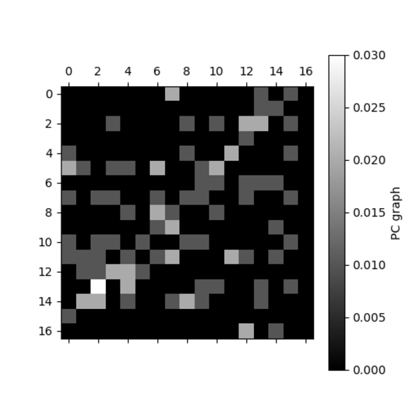
In Gupta et al. [16] a chaos game is used to represent a time series as a PC plot and compare similarities and dissimilarities in different time frame such as the global pandemic of COVID-19. More precisely, the author consider the set X=[0,1]2X=[0,1]^{2} as the base space and the four linear contractions

{τA​(x,y)=(0.5​x,0.5​y)τB​(x,y)=(0.5​x+0.5,0.5​y)τC​(x,y)=(0.5​x,0.5​y+0.5)τD​(x,y)=(0.5​x+0.5,0.5​y+0.5)\left\{\begin{array}[]{l}\tau_{A}(x,y)=(0.5x,0.5y)\\ \tau_{B}(x,y)=(0.5x+0.5,0.5y)\\ \tau_{C}(x,y)=(0.5x,0.5y+0.5)\\ \tau_{D}(x,y)=(0.5x+0.5,0.5y+0.5)\end{array}\right. (10)

so (X,τθ)θ∈Θ,Θ={A,B,C,D}(X,\tau_{\theta})_{\theta\in\Theta},\Theta=\{A,B,C,D\}, is a classic contractive system whose attractor is XX itself. Consider the identification:
A – if the market falls more than 0.01% of the previous value,
B – if the market falls less than 0.01% of the previous value,
C – if the market gains less than 0.01% of the previous value and
D – if the market gains more than 0.01% of the previous value,
in this way the time series of length NN associated to a certain economic indicator is translated in to a genetic sequence

γ=(D​A​C​C​A​D​C​D​A​C​D​C​…​A​A​C​C​B​A​D​D)∈ΘN.\gamma=(DACCADCDACDC...AACCBADD)\in\Theta^{N}.

Fixed an arbitrary initial point Z0=(x0,y0)=(0.5,0.5)Z_{0}=(x_{0},y_{0})=(0.5,0.5) the chaos game consists in iterating (x0,y0)(x_{0},y_{0}) by each map Z1=(x1,y1)=τD(x0,y0),Z2=(x2,y2)=τA(x1,y1),Z3=(x3,y3)=τC(x2,y2),….Z_{1}=(x_{1},y_{1})=\tau_{D}(x_{0},y_{0}),Z_{2}=(x_{2},y_{2})=\tau_{A}(x_{1},y_{1}),Z_{3}=(x_{3},y_{3})=\tau_{C}(x_{2},y_{2}),.... according to γ\gamma. Considering M≥2M\geq 2 and the diadic partition of XX given by

⋃γ′∈ΘMτγM′(⋯(τγ1′(X))),\bigcup_{\gamma^{\prime}\in\Theta^{M}}\tau_{\gamma^{\prime}_{M}}(\cdots(\tau_{\gamma^{\prime}_{1}}(X))),

the PC plot WW is a grey scale picture where the color of the each individual part Λ=τγM′(⋯(τγ1′(X)))\Lambda=\tau_{\gamma^{\prime}_{M}}(\cdots(\tau_{\gamma^{\prime}_{1}}(X))) is the frequency of visits of the chaos game orbit {Zj,j≥0}\{Z_{j},j\geq 0\} to Λ\Lambda that is,

W(Λ)=1N♯{j=0,…,N−1|Zj∈Λ}∼μ(Λ).W(\Lambda)=\frac{1}{N}\,\sharp\{j=0,...,N-1\,|\,Z_{j}\in\Lambda\}\sim\mu(\Lambda).

Obviously, νN=∑ΛW⁡(Λ)​δ(xΛ,yΛ)\nu_{N}=\sum_{\Lambda}W(\Lambda)\delta_{(x_{\Lambda},\,y_{\Lambda})}, where (xΛ,yΛ)∈Λ(x_{\Lambda},\,y_{\Lambda})\in\Lambda is arbitrary, is a discrete probability and, if μ⁡(∂(Λ))=0\mu(\partial(\Lambda))=0 then by the EET ([13], Corollary 2), when N→∞N\to\infty, νN\nu_{N} converge in distribution to the invariant measure μ\mu for the IFS with probabilities (X,τθ,pθ)θ∈Θ(X,\tau_{\theta},p_{\theta})_{\theta\in\Theta}, where pA,pB,pC,pDp_{A},p_{B},p_{C},p_{D} are the relative frequency of each symbol A,B,C,DA,B,C,D in γ\gamma, respectively.
For instance, if N=100N=100 and if a certain time series produces the genetic sequence

γ=(A,A,D,D,A,…,A,D,B,C,C,B,A,D)∈{A,B,C,D}100,\gamma=(A,A,D,D,A,...,A,D,B,C,C,B,A,D)\in\{A,B,C,D\}^{100},

we obtain the frequencies [pA,pB,pC,pC]=[0.39, 0.17, 0.15, 0.29][p_{A},p_{B},p_{C},p_{C}]=[0.39,\,0.17,\,0.15,\,0.29], and considering M=4M=4 we obtain the following PC plot

Refer to caption
Figure 1: PC plot where each square represents one element Λ\Lambda of the diadic partition and grey scale value 0≤1N♯{j=0,…,N−1|Zj∈Λ}≤10\leq\frac{1}{N}\,\sharp\{j=0,...,N-1\,|\,Z_{j}\in\Lambda\}\leq 1.

which is an approximation for the invariant measure μ\mu of the associated IFS with probabilities [0.39, 0.17, 0.15, 0.29][0.39,\,0.17,\,0.15,\,0.29].

In order to generalize this idea we need to consider an infinite compact continuous range of values of the economic indicator, such as Θ=[0%,100%]\Theta=[0\%,100\%], instead of taking only four values Θ={A,B,C,D}\Theta=\{A,B,C,D\}. Also, it is not reasonable to suppose that the probability of a change of θ%\theta\% in the indicator is independent of the current state of the indicator: the distribution of the occurrence of θ∈[0%,100%]\theta\in[0\%,100\%], given the current state Z∈XZ\in X must be a measure of probability qZ​(⋅)q_{Z}(\cdot) over [0%,100%][0\%,100\%]. Therefore, we believe the theory developed in the previous sections should be used when making this generalization.

Aknowledgement: We would like to thanks Prof. Leandro Cioletti whose contribution on the related preprint [8] was fundamental to establish the tools and ideas that we now generalize in our work.

References

  • [1] D. Aguiar, L. Cioletti, and R. Ruviaro. A variational principle for the specific entropy for symbolic systems with uncountable alphabets. Mathematische Nachrichten, 291(17-18):2506–2515, 2018.
  • [2] Luigi Ambrosio, Nicola Gigli, and Giuseppe Savaré. Gradient flows in metric spaces and in the space of probability measures. Springer Science & Business Media, Basel, 2008.
  • [3] Michael F. Barnsley and Stephen Demko. Iterated function systems and the global construction of fractals. Proceedings of the Royal Society of London. A. Mathematical and Physical Sciences, 399(1817):243–275, 1985.
  • [4] Michael F. Barnsley, Stephen G. Demko, John H. Elton, and Jeffrey S. Geronimo. Invariant measures for markov processes arising from iterated function systems with place-dependent probabilities. In Annales de l’IHP Probabilités et statistiques, volume 24, pages 367–394, 1988.
  • [5] Vasile Berinde and Madalina Pacurar. The role of the Pompeiu-Hausdorff metric in fixed point theory. Creative Mathematics and Informatics, 22(2):143–150, 2013.
  • [6] D. Charalambos and Border Aliprantis. Infinite Dimensional Analysis: A Hitchhiker’s Guide. Springer-Verlag Berlin and Heidelberg GmbH & Company KG, 3 edition, 2006.
  • [7] Ion Chiţescu, Loredana Ioana, and Radu Miculescu. Type A sets and the attractors of infinite iterated function systems. Results Math., 66(3-4):511–524, 2014.
  • [8] Leandro Cioletti and Elismar R. Oliveira. Thermodynamic formalism for iterated function systems with weights, Preprint, arXiv:1707.01892, 2017.
  • [9] Leandro Cioletti and Elismar R. Oliveira. Applications of variable discounting dynamic programming to iterated function systems and related problems. Nonlinearity, 32(3):853, 2019.
  • [10] Claude Dellacherie and Paul-André Meyer. em Probabilities and potential, Vol. 29 of North-Holland mathematics studies, 1978.
  • [11] J. L. Doob, Asymptotic properties of Markoff transition prababilities Trans. Amer. Math. Soc. 63 (1948), 393–421.
  • [12] Dan Dumitru. Attractors of infinite iterated function systems containing contraction type functions. An. Ştiinţ. Univ. Al. I. Cuza Iaşi, Mat. NS, 59:281–298, 2013.
  • [13] John H. Elton. An ergodic theorem for iterated maps. Ergodic Theory and Dynamical Systems, 7(4):481–488, 1987.
  • [14] Ai Hua Fan and Ka-Sing Lau. Iterated function system and ruelle operator. Journal of mathematical analysis and applications, 231(2):319–344, 1999.
  • [15] Henning Fernau. Infinite iterated function systems. Math. Nachr., 170:79–91, 1994.
  • [16] Aman Gupta, Cyril Shaju, Pratibha & Kamal. A study of the international stock market behavior during COVID-19 pandemic using a driven iterated function system. Computational economics, pages 1–12, 2021.
  • [17] Gertruda Gwóźdź-Lukawska and Jacek Jachymski. The Hutchinson-Barnsley theory for infinite iterated function systems. Bulletin of the Australian Mathematical Society, 72(3):441–454, 2005.
  • [18] Pawel Hanus, R. Mauldin, and Mariusz Urbański. Thermodynamic formalism and multifractal analysis of conformal infinite iterated function systems. Acta Mathematica Hungarica, 96(1-2):27–98, 2002.
  • [19] Martial R. Hille. Remarks on limit sets of infinite iterated function systems. Monatsh. Math., 168(2):215–237, 2012.
  • [20] John E. Hutchinson. Fractals and self similarity. Indiana University Mathematics Journal, 30(5):713–747, 1981.
  • [21] Antti Käenmäki. On natural invariant measures on generalised iterated function systems. Ann. Acad. Sci. Fenn. Math, 29(2):419–458, 2004.
  • [22] Andrzej Lasota, Józef Myjak and Tomasz Szarek. Markov operators with a unique invariant measure. Journal of mathematical analysis and applications, 276(1), 343–356, 2002.
  • [23] Artur O. Lopes, Jairo K. Mengue, Joana Mohr, and Rafael R. Souza. Entropy and variational principle for one-dimensional lattice systems with a general a priori probability: positive and zero temperature. Ergodic Theory and Dynamical Systems, 35(6):1925–1961, 2015.
  • [24] Artur O. Lopes and Elismar R. Oliveira. Entropy and variational principles for holonomic probabilities of IFS. Discrete & Continuous Dynamical Systems, 23(3):937–955, 2009.
  • [25] Richard Daniel Mauldin and Mariusz Urbański. Parabolic iterated function systems. Ergodic Theory and Dynamical Systems, 20(5):1423–1447, 2000.
  • [26] Richard Daniel Mauldin and Mariusz Urbański. Dimensions and measures in infinite iterated function systems. Proc. London Math. Soc. (3), 73(1):105–154, 1996.
  • [27] Alexandru Mihail and Radu Miculescu. The shift space for an infinite iterated function system. Math. Rep. (Bucur.), 11(61)(1):21–32, 2009.
  • [28] Manuel Morán. Hausdorff measure of infinitely generated self-similar sets. Monatsh. Math., 122(4):387–399, 1996.
  • [29] David Ruelle. A variational formulation of equilibrium statistical mechanics and the Gibbs phase rule. Communications in Mathematical Physics, 5(5):324–329, 1967.
  • [30] David Ruelle. Statistical mechanics of a one-dimensional lattice gas. Communications in Mathematical Physics, 9(4):267–278, 1968.
  • [31] Károly Simon, Boris Solomyak, and Mariusz Urbański. Invariant measures for parabolic ifs with overlaps and random continued fractions. Transactions of the American Mathematical Society, 353(12):5145–5164, 2001.
  • [32] Örjan Stenflo. Uniqueness of invariant measures for place-dependent random iterations of functions. In Fractals in Multimedia, pages 13–32. Springer, 2002.
  • [33] Peter Walters. Ruelle’s operator theorem and g-measures. Transactions of the American Mathematical Society, 214:375–387, 1975.