Black hole encircled by a thin disk: fully relativistic solutionDedicated to our teacher, colleague and friend, Professor Oldřich Semerák, on the occasion of his 60th orbit around the Sun. Oldřich’s well-known lectures – famous not only among us (former) students of ‘math-phys’ in Prague – were the first impulse that led us to devote our studies to general relativity.Wolfram Mathematica 13

Black holes are once again in the spotlight of astrophysical interest thanks to the unprecedented improvement of imaging techniques in the last couple of years. The key aspect in imaging a black hole shadow is the presence of accreting matter. Having nonvanishing angular momentum, such matter usually forms an accretion disk inspiraling into the black hole. The usual simplification of this model is neglecting the disk self-gravitation because the real accretion disks are supposed to be much lighter than the central black hole. However, in many situations, this is not necessarily true, and many disk properties such as stability and positions of significant orbits are sensible to the gravitational field. Thus, we should include also the disk’s own gravity in our considerations.

Nevertheless, the complexity of Einstein’s equations makes the treatment in the most general case almost impossible using just analytical methods. We have to simplify the problem at some point. A great source of difficulties is the presence of overall net rotation and the resulting dragging effects. But if the rotation can be neglected or if it is compensated by e.g. two equal counter-orbiting streams, the situation is much simpler. Namely, any static and axially symmetric vacuum spacetime (or any non-empty spacetime where the condition $T^{\rho}_{\rho}+T^{z}_{z}=0$ for the stress-energy tensor holds) can always be described by a Weyl-type metric

where $t,\rho,\phi,z$ are Weyl coordinates and functions $\nu,\lambda$ depend solely on $\rho,z$. Outside sources, the function $\nu$ satisfies 3 dimensional Laplace equation (therefore $\nu$ is the counterpart of Newtonian gravitational potential), and for $\lambda$ we have

Just like in electrostatics and Newtonian gravity, in order to find the external gravitational field in GR, we have to solve the Laplace (or Poisson) equation. But that is only the (Newtonian) part of the whole story. The field is not fully determined only by the potential – there is also the second metric function $\lambda$ which influences the geometry in the meridional $(\rho,z)$ plane. This feature can significantly deviate from the Newtonian picture. Moreover, while the linearity of the Laplace equation means a considerate simplification in obtaining the field generated by more than one individual source (the potentials simply add up), the non-linear nature of Einstein’s equations exhibits itself in the second metric function $\lambda$.

The first static superposition of a black hole and a thin disk (inverted solution of Morgan & Morgan 1969) was considered by Lemos & Letelier 1993 and further studied in e.g. Semerák 2003. Later, Semerák 2004 found a potential of a disk with a general power-law density profile in terms of infinite series and studied its properties when superposed with a black hole. In a recent revision of this topic in Kotlařík et al. 2022, we provided this result in closed-form. All these disks are thin, infinite, and have an inner rim, where higher derivatives of curvature are singular. Also, only the Newtonian part (i.e. gravitational potential) of the superposition is given analytically; the second metric function $\lambda$, if needed, has to be solved numerically using (2). Here, we provide exact full relativistic solutions describing superposition of a black hole with a disk which extends from the horizon to infinity. The fields are everywhere regular, and both metric functions of the superposition are obtained in closed-forms. It may seem inappropriate to consider disks which reach down to the horizon, since the stationary horizons cannot host any matter, and since quasi-stationary accretion disks are assumed to end somewhere about the innermost stable circular orbit. However, (i) our disk densities drop to zero towards the black hole, so there is really no matter at the very horizon, and (ii) the accretion disks around astrophysical black holes indeed continue towards the horizon (at least partially), though their matter is infalling there rather than orbiting in a quasi-circular regime. (Below the last stable orbit, the disk should not be interpreted in terms of stationary circular motion.) Hence, it is in fact more realistic to model the gravitational field of an accreting black hole employing a disk that does have a certain modest density going down to the horizon.

Before we proceed further, let us also mention other exact static black-hole–disk superposition, where both non-trivial metric functions have been obtained. González et al. 2009 found a family of infinite disks with an inner edge suitable for the superposition with a black hole. However, Gleiser 2012 showed that the disks have problematic physical interpretation. More realistic result was obtained by Vieira 2020 using ‘displace, cut and reflect’ method applied to solutions of $N$ black holes (singular rods in Weyl coordinates) arranged in a linear chain on the symmetry axis.

The paper is organized as follows. First, in the Section II, we review a family of thin infinite (in extent) – but of finite mass – disks due to Kuzmin 1956 and Toomre 1963, which were later studied in the context of GR by Bičák et al. 1993. Then, by inversion (Kelvin transformation) of the potential with respect to some Weyl radius, we find the potential describing, again, thin infinite disks of finite mass, but in this case, their surface densities are zero at $\rho=0$. The same potential has been found before, as a special case, by Vogt & Letelier 2009 via superposition within the Kuzmin-Toomre family. Here, we contribute to this result with the second metric function $\lambda$ and thus obtain full relativistic solutions describing inverted Kuzmin-Toomre disks. Moreover, in Section III, we also provide exact solutions of $\lambda$ to all ‘single rings’ found in Vogt & Letelier 2009 – disks similar to the inverted Kuzmin-Toomre ones, but their surface density falls faster. All these disks are suitable for the superposition with a central black hole, thanks to their ‘annular’ character. This is done in Sec. IV where, again, both metric functions of the black-hole–disk superposition are derived. In the subsequent Sections V and VI we study some properties of the resulting gravitational field, namely the disk’s influence on the black-hole horizon, radial profiles of densities, pressures and circular speeds in the equatorial plane. Finally, in Section VII we make several concluding remarks.

The $n$-order Kuzmin-Toomre disk, $n\geq 0$, is described by the potential (Kuzmin 1956; Toomre 1963; Evans & de Zeeuw 1992; Bičák et al. 1993)

where we have denoted

$\mathcal{M}$ stands for the total mass of the disk, and $P_{k}$ are Legendre polynomials. The corresponding Newtonian density¹¹ 1 $\nu$ is the solution of $\Delta\nu(\rho,z)=4\pi w(\rho)\delta(z)$, where $\Delta$ is standard Laplace operator in cylindrical coordinates, $\delta$ is delta distribution. reads

Such a potential can be constructed by considering some mass distribution along the negative half of the axis $z<0$, then cutting the solution along the equatorial plane $z=0$ and reflecting its upper part $z>0$ to the negative part $z<0$ of the axis – the so-called ‘displace, cut and reflect’ method (Kuzmin 1956; Vieira 2020). The resulting field is then symmetric with respect to the equatorial plane $z=0$ and given by

For Kuzmin-Toomre solution, the weight function $W$ is a distribution given by some combination of the derivatives of delta distribution (Bičák et al. 1993). Note that in paper Bičák et al. 1993, the weight function given in (2.23) does not in fact correspond to the Kuzmin-Toomre disks, but rather to the solution obtained by inversion with respect to $\rho=b$, only with different normalization – see the explicit treatment below.

Inverted Kuzmin-Toomre disks are obtained by performing an inversion with respect to²² 2 Performing the inversion around an arbitrary radius $a$ leads to the same density profile just with different Weyl distance $b\longrightarrow a^{2}/b$. $b$ (Kelvin transformation), i.e. the coordinate transformation

and the respective potential and density transformation

The inversion of (3), after a suitable rearrangement of the sum, is again separable in $r_{b}$ and $\cos\theta_{b}$ and can be easily derived from (3) by (i) replacing $b\rightarrow-b$, (ii) multiplying each term by the hypergeometric function $\operatorname{{\vphantom{\mathnormal{F}}}{}_{2}\kern-0.5pt\mathnormal{F}_{1}}(1+k,k-n;k-2n;2)$, (iii) fixing the normalization, so the total mass of the disk is still $\mathcal{M}$. The inverted potential reads³³ 3 Note that $$\frac{(2n-k)!}{2^{n-k}(n-k)!}\operatorname{{\vphantom{\mathnormal{F}}}{}_{2}\kern-0.5pt\mathnormal{F}_{1}}(1+k,k-n;k-2n;2)=\sum_{j=k}^{n}\binom{j}{k}\frac{(2n-j)!}{2^{n-j}(n-j)!}\;.$$

and the corresponding Newtonian density profile

Similarly as the original Kuzmin-Toomre disks (3), the $n$th-order potential follows also from the recurrence relation

The shape of the disk potential along the equatorial plane and along the axis is illustrated in Fig. 2. The Newtonian surface densities are depicted in Fig. 1.

The second metric function $\lambda_{n}$ can be also obtained following the same steps as Bičák et al. 1993. They consist in rewriting the derivatives in Eq. (2) in terms of $(r_{b},\theta_{b})$ and integrating from $r_{b}$ to the infinity requiring $\lambda\rightarrow 0$ when $r_{b}\rightarrow\infty$. Then

where

Vogt & Letelier 2009 obtained a broader family of disks by a superposition within the original Kuzmin-Toomre disks. They took

where $W^{(m,n)}$ is a normalization factor dependent only on $m,n$. Resulting disks are again of infinite extent with the surface density

which behaves as $\mathcal{O}(\rho^{-2m-3})$ at infinity, thus the total mass of each disk is again finite. We fix $W^{(m,n)}$, so the total mass of the disk is still $\mathcal{M}$, more precisely

For $m=0$, we get the inverted Kuzmin-Toomre disks, which we diskussed in the previous section. disks of higher $m$ can be obtained using a recurrence relation

After substitution of the Kuzmin-Toomre potential into (16) the double sum can be rearranged and performed over the $k$ index. It leads to

where we have already substituted $W^{(m,n)}$ from (18) and

where $\operatorname{{\vphantom{\mathnormal{F}}}{}_{3}\kern-0.5pt\mathnormal{F}_{2}}$ is the generalized hypergeometric function.

The second metric function $\lambda$ is again of the same structure (12) as the original or inverted Kuzmin-Toomre disks, but now

while the polynomials $\mathcal{P}_{k,l}$ are the same as in (12). A shorter expression can be found by the off-diagonal re-summation

where $P_{u}\equiv P_{u}(|\cos\theta_{b}|)$ are the Legendre polynomials and we set $\mathcal{Q}_{u}^{(m,n)}=0$ for $u>m+n$. For the inverted Kuzmin-Toomre disks (i.e. $m=0$) the coefficients are reduced $\mathcal{Q}_{u}^{(0,n)}=\frac{(-1)^{u}}{(2n+1)!!}\frac{(2n-u)!}{2^{n-u}(n-u)!}\operatorname{{\vphantom{\mathnormal{F}}}{}_{2}\kern-0.5pt\mathnormal{F}_{1}}(1+u,u-n;u-2n;2)$.

Newtonian density profiles of several Vogt-Letelier disks are plotted in Fig. 3 and the behavior of disks’ potentials in the equatorial plane and on the axis is illustrated in Fig. 4.

All Vogt-Letelier disks have a clear ‘annular’ character – their densities are exactly zero in the centre $(\rho=0,z=0)$. Hence, it is physically reasonable to make a static superposition of such a disk with a black hole. In Weyl coordinates, the Schwarzschild black hole of the mass $M$ is a singular rod placed on the axis $(\rho=0,|z|\leq M)$ producing gravitational field described by

where $d_{1,2}\equiv\sqrt{\rho^{2}+(|z|\mp M)^{2}}$. Then, the disk starts at the black-hole horizon, but the density drops to zero sufficiently quickly there. Due to the linearity of Laplace equation, the superposition of gravitational potentials is a simple sum of the individual sources, i.e. $\nu=\nu_{\text{Schw}}+\nu_{\text{disk}}$. The non-linearity of the Einstein equations manifests itself in the second metric function $\lambda$ which does not superpose that simply. In fact, for two individual sources, a black hole and a disk, we can write $\lambda=\lambda_{\text{Schw}}+\lambda_{\text{disk}}+\lambda_{\text{int}}$, where $\lambda_{\text{Schw}}$ and $\lambda_{\text{disk}}$ are contributions from the black hole and the disk alone (thus satisfying (2) with just $\nu_{\text{Schw}}$ and $\nu_{\text{disk}}$ respectively) and $\lambda_{\text{int}}$ is an ‘interaction’ term for which

Notice that these conditions are already linear in $\nu_{\text{disk}}$, i.e. if the potential of the disk is a sum of two components then also $\lambda$ must add in the same way. Hence, $\lambda_{\text{int}}$ satisfies the same recurrence relations (11) for the inverted Kuzmin-Toomre disks and (19) for Vogt-Letelier disks of higher $m$, namely

Superposition with a black hole is best represented in Schwarzschild coordinates⁴⁴ 4 Note that Schwarzschild coordinates $(r,\theta)$ are different from those coordinates with subscript $b$ used in disks’ potentials. $(r,\theta)$ introduced by

In these coordinates the black-hole horizon is rendered really spherical (at $r=2M$), the Schwarszchild contribution becomes

and the metric of the superposition reads

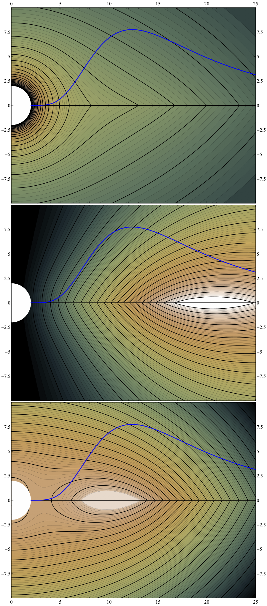
where $\lambda_{\text{ext}}\equiv\lambda-\lambda_{\text{Schw}}=\lambda_{\text{disk}}+\lambda_{\text{int}}$. The resulting field is illustrated in Fig. 6 on several contour plots. In Fig. 5, we show radial plots of $\lambda_{\text{ext}}$ in the equatorial plane.

Even though the horizon of the black hole always lies at the Schwarzschild radius $r=2M$ and remains ‘spherical’ in the Schwarszchild coordinates, its intrinsic geometry changes due to the presence of the surrounding matter distribution. At any given (coordinate) time, the horizon is a 2D-surface $(t=\text{konst},r=2M)$ with an induced metric

where $\nu^{\text{H}}_{\text{disk}}$ is the limit of the disk potential at the horizon ($r\rightarrow 2M$), and where we have already used solution $\lambda^{\text{H}}(\theta)=2\nu^{\text{H}}(\theta)-2\nu^{\text{H}}(\theta=0)$ valid on the horizon (for any static or even stationary axially symmetric spacetime). For isometric embedding to Euclidean 3-space, we use the method by Smarr 1973. It consists in rewriting the 2-metric in terms of the coordinate $\mu=\cos\theta$, i.e.

where

Then, the isometric embedding of the horizon 2-surface in three-dimensional Euclidean space $(x,y,z)$ is given by

See Fig. 7 for the numerical results. Another useful quantity for any 2D surface is its Gauss curvature $\mathcal{K}\equiv\frac{{}^{(2)}R}{2}$, where ${}^{(2)}R$ is the corresponding 2D scalar curvature. For the metric (32), we have

The Gauss curvature is plotted against $\mathcal{M}$ and $b$ in Fig. 8. When the Gauss curvature turns negative, the horizon is not globally embeddable into Euclidean 3-space. Both, the embedding and the Gauss curvature, shows flattened horizon in the direction of the disk.

Two rather simple physical interpretations of any static thin disks are (i) a single component ideal fluid with a certain surface density $\sigma$ and an azimuthal pressure $P$, or (ii) two identical counter-orbiting dust streams with proper surface densities $\sigma_{+}=\sigma_{-}\equiv\frac{\sigma}{2}$ following circular geodesics. Both characteristics follow from the diskontinuities of normal derivatives of the field over the equatorial plane

where $w(\rho)$ is the Newtonian density (10), or (17). The second interpretation is possible only when $\sigma,P\geq 0$.

We have found full metric describing static and axially symmetric superposition of a black hole and a thin disk. The disks we considered have finite mass, have no radial pressure and extend from the black-hole horizon to infinity. They also have no edges, so the field is regular everywhere outside the horizon, yet the disks surface densities fall off sufficiently quickly at both extremes $\rho=0$ and $\rho\rightarrow\infty$. In particular, we have used disks resulting from the inversion (Kelvin transformation) of Kuzmin-Toomre solutions, as well as ‘simple’ disks due to Vogt & Letelier 2009 (of which the inverted Kuzmin-Toomre disks are a distinct subclass). Both metric functions are given analytically and in closed-forms. The gravitational field is illustrated in plots of the metric functions and profiles of densities, azimuthal pressures and circular velocities. The black-hole horizon was found distorted due to the presence of the disk (flattened in the direction of the disk) which is in agreement with many previous results, e.g. Semerák 2004; Semerák 2003; Semerák et al. 2001, or, in the stationary case, Kotlařík et al. 2018.

References

- Bičák et al. (1993) Bičák, J., Lynden-Bell, D., & Pichon, C. 1993, MNRAS, 265, 126, doi: 10.1093/mnras/265.1.126
- Evans & de Zeeuw (1992) Evans, N. W., & de Zeeuw, P. T. 1992, MNRAS, 257, 152, doi: 10.1093/mnras/257.1.152
- Gleiser (2012) Gleiser, R. J. 2012, Phys. Rev. D, 85, 028501, doi: 10.1103/PhysRevD.85.028501
- González et al. (2009) González, G. A., Gutiérrez-Piñeres, A. C., & Viña-Cervantes, V. M. 2009, Phys. Rev. D, 79, 124048, doi: 10.1103/PhysRevD.79.124048
- Kotlařík et al. (2022) Kotlařík, P., Kofroň, D., & Semerák, O. 2022, ApJ, 931, 161, doi: 10.3847/1538-4357/ac6027
- Kotlařík et al. (2018) Kotlařík, P., Semerák, O., & Čížek, P. 2018, Phys. Rev. D, 97, doi: 10.1103/PhysRevD.97.084006
- Kuzmin (1956) Kuzmin, G. G. 1956, Astr. Zh., 33, 27
- Lemos & Letelier (1993) Lemos, J. P. S., & Letelier, P. S. 1993, CQGra, 10, L75, doi: 10.1088/0264-9381/10/6/003
- Morgan & Morgan (1969) Morgan, T., & Morgan, L. 1969, Phys. Rev., 183, 1097, doi: 10.1103/PhysRev.183.1097
- Semerák (2003) Semerák, O. 2003, CQGra, 20, 1613, doi: 10.1088/0264-9381/20/9/302
- Semerák (2004) Semerák, O. 2004, CQGra, 21, 2203, doi: 10.1088/0264-9381/21/8/019
- Semerák et al. (2001) Semerák, O., Zellerin, T., & Žáček, M. 2001, MNRAS, 322, 207, doi: 10.1046/j.1365-8711.2001.03814.x
- Smarr (1973) Smarr, L. 1973, Phys. Rev. D, 7, 289, doi: 10.1103/PhysRevD.7.289
- Toomre (1963) Toomre, A. 1963, ApJ, 138, 385, doi: 10.1086/147653
- Vieira (2020) Vieira, R. S. 2020, CQGra, 37, doi: 10.1088/1361-6382/aba99b
- Vogt & Letelier (2009) Vogt, D., & Letelier, P. S. 2009, MNRAS, 396, 1487, doi: 10.1111/j.1365-2966.2009.14803.x