Nonlinear Set Membership Filter with State Estimation Constraints via Consensus-ADMM^footnoteinfo

The basic idea of the SMF is to obtain a feasible solution set containing the true state according to the dynamic system, measurements, bounded noises, and other information about the state [11, 13]. Specifically, suppose the initial state $x_{0}$ belongs to a given set ${\mathcal{Y}}_{0}$. The objective of the SMF is to determine a minimum volume state bounding set ${\mathcal{Y}}_{k+1}$ based on ${\mathcal{Y}}_{k}$, the dynamic system, measurements, bounded noises, and other information at time step $k+1$.

The SMF is subdivided into the prediction and the measurement update step. In the prediction step at time $k+1$, a predicted state bounding set ${\mathcal{Y}}_{k+1|k}$ is determined as the minimum volume set according to the state bounding set ${\mathcal{Y}}_{k}$, the state transform equation, the process noise information, and other information. In the measurement update step at time $k+1$, a state bounding set ${\mathcal{Y}}_{k+1}$ is determined as the minimum volume set according to the predicted state bounding set ${\mathcal{Y}}_{k+1|k}$, the measurement equation, the measurements, the measurement noise information, and other information.

In general, two basic set representations are used in the SMF: polytopes of various types (e.g., general polytopes [30], boxes [31], zonotopes [32], parallelotopes [33], and rectangular polytopes [34]) and ellipsoid [35]. Polytopes can give arbitrarily close approximations to any convex set, but the number of vertices can grow prohibitively large [30]. The complexity of the ellipsoidal representation is quadratic in the dimension of the set since its size, shape, and location can be determined uniquely by its center and shape matrix. In addition, it is possible to single out a set approximating ellipsoid that is optimal to some given criterion or a combination of them [35]. Therefore, we focus on the ellipsoid approach in this paper, and some preliminaries of the ellipsoid are provided as follows.

Definition 1. A set ${\mathcal{E}}\subset\mathbb{R}^{n}$ satisfying the following form is called an ellipsoid:

where $e\in\mathbb{R}^{n}$ and $E\succ 0$ are the center and the shape matrix of $\mathcal{E}$, respectively.

The “size” of an ellipsoid ${\mathcal{E}}(e,E)$ can be expressed as a function $J(E)$ of the shape matrix $E$ [13]. In this paper, we choose the most common ways to measure the “size” of an ellipsoid, which are the trace function ($J(E)=tr(E)$, which corresponds to the sum of squares of semiaxes lengths of $\mathcal{E}(e,E)$) and logdet function ($J(E)=\log\det(E)$, which corresponds to the volume of $\mathcal{E}(e,E)$), respectively [17]. The problem of finding the smallest ellipsoidal outer approximation of a bounded set $\mathcal{X}\subset\mathbb{R}^{n}$ on the trace or logdet criterion can be described as:

Definition 2. The Minkowski sum of two ellipsoids ${\mathcal{E}}_{1}$ and ${\mathcal{E}}_{2}$ is defined as:

Definition 3. The intersection of two ellipsoids ${\mathcal{E}}_{1}$ and ${\mathcal{E}}_{2}$ is defined as:

Next, we briefly introduce the consensus-ADMM method used in this paper [36, 37]. Consider the problem:

where $x\in\mathbb{R}^{n}$, the objective function is the sum of the objective terms $\Pi_{i}(x):\mathbb{R}^{n}\to\mathbb{R}\cup\{+\infty\},~i=1,...,\omega$. Problem (1) can be reformulated as a consensus form by introducing $\omega$ auxiliary variables $z_{i}\in\mathbb{R}^{n},~i=1,...,\omega$:

then the consensus-ADMM iterates at iteration $t$ for this problem are:

where $\rho>0$ is the penalty parameter, $\lambda_{i}$ is the Lagrange multiplier, and $x^{t}$ and $\lambda_{i}^{t}$ are the updates obtained in the $t$-th iteration and $z_{i}^{t+1}$, $x^{t+1}$, and $\lambda_{i}^{t+1}$ are the updates obtained in the $t+1$-th iteration, respectively. In the consensus-ADMM iterates, $z_{i}$, $x$, and $\lambda_{i}$ are updated in an alternating fashion, and the $z_{i}$-minimization step is independently for each $i$. More details on the consensus-ADMM method can be seen in [36]. The consensus-ADMM algorithm is a very intuitive algorithm with several advantages [36, 37]. First, the update of the variables $z_{i}$ can be implemented in parallel since they are independent of each other. Next, each update can be efficient for the high-dimensional but sparse datasets by splitting the cost functions. Moreover, the consensus-ADMM method converges if the problem is convex.

Consider the nonlinear dynamic system:

where $k$ denotes the time step, $x_{k}\in\mathbb{R}^{n}$ is the system state, $y_{k}\in\mathbb{R}^{m}$ is the measurement, $f_{k}(x_{k})$ and $h_{k}(x_{k})$ are nonlinear uniformly continuous and differentiable process function and measurement function of $x_{k}$, respectively. The process noise $w_{k}\in\mathbb{R}^{n}$ and the measurement noise $v_{k}\in\mathbb{R}^{m}$ are assumed to be restricted in given ellipsoidal sets $W_{k}={\mathcal{E}}(0,Q_{k})$ and $V_{k}={\mathcal{E}}(0,R_{k})$, respectively. In many practical scenarios, the state estimation $\hat{x}_{k}$ is expected to be localized in specific subspace [24]. In particular, we consider the following equality state estimation constraint:

where $g_{k}(\hat{x}_{k})$ is a continuously differentiable function.

Suppose the initial state $x_{0}$ belongs to ${\mathcal{E}}_{0}(\hat{x}_{0},P_{0})$. The objective of this paper is to design a SMF that determines a minimum volume state bounding ellipsoid ${\mathcal{E}}_{k+1}(\hat{x}_{k+1},P_{k+1})$ based on ${\mathcal{E}}_{k}(\hat{x}_{k},P_{k})$, the dynamic system, measurements, bounded noises, and constraint at time step $k+1$.

In this subsection, we consider the prediction step of the proposed nonlinear SMF. Let ${\mathcal{E}}_{k}(\hat{x}_{k},P_{k})$ and ${\mathcal{E}}_{k+1|k}(\hat{x}_{k+1|k},P_{k+1|k})$ denote the state bounding ellipsoid of $x_{k}$ and the predicted ellipsoid of $x_{k+1}$, respectively. According to the uniform continuity of $f_{k}$, we have that ${\mathcal{F}}_{k}=\{f_{k}(x_{k}):x_{k}\in{\mathcal{E}}_{k}\}$ is a bounded compact set. Therefore, a minimum volume ellipsoid ${\mathcal{E}}_{f_{k}}(\hat{x}_{f_{k}},P_{f_{k}})$ containing ${\mathcal{F}}_{k}$ can be obtained by solving:

From (2), we have $x_{k+1}\in{\mathcal{E}}_{f_{k}}\oplus W_{k}$. Thus, the predicted state bounding ellipsoid at time $k+1$ can be obtained by solving:

Remark 1. Theorem 4.2 in [17] and (6) show that the shape matrix of ${\mathcal{E}}_{k+1|k}$ has the following form:

where $\tau_{k}>0$. The selection of $\tau_{k}$ determines the property of ${\mathcal{E}}_{k+1|k}$, and the problem (6) can be reformulated as $min_{\tau_{k}>0}J(P_{k+1|k}(\tau_{k}))$. Especially, if $J(P_{k+1|k})=tr(P_{k+1|k})$, then the optimal solution to this optimization problem is $\tau_{k}=\sqrt{\frac{tr(P_{f_{k}})}{tr(Q_{k})}}$.

The following lemma shows the condition under which the state prediction satisfies the estimation constraint.

Lemma 1. The state prediction $\hat{x}_{k+1|k}$ satisfies the constraint (4) if and only if $\hat{x}_{f_{k}}$ satisfies (4).

Proof: See Appendix A. $\square$

Based on the optimization problem (5) and Lemma 1, in order to make the predicted state located in the constraint subspace, the problem of determining the predicted state bounding ellipsoid has been transformed into:

The optimization problem (8) is a SIP problem that includes two variables and infinite inequality constraints, and it is not jointly convex in the two variables. Therefore, the problem (8) is difficult to solve, and we provide a consensus-ADMM-based method to handle it in Section 4.

Subsequently, we consider the measurement update step of the proposed filter. Based on the predicted ellipsoid and the measurement at time $k+1$, we seek the minimum volume state bounding ellipsoid ${\mathcal{E}}_{k+1}(\hat{x}_{k+1},P_{k+1})$ with the center $\hat{x}_{k+1}$ satisfying the estimation constraint (4).

For the convenience of the analysis, we assume that there exists a continuous inverse function $h_{k+1}^{-1}$ for the nonlinear function $h_{k+1}$. Thus, the measurement function is reformulated as:

Remark 2. Equation (9) uses the information about the inverse function of the measurement function to estimate the state instead of linearizing the nonlinear system, thus leading to more accurate state estimates [16]. In general, the assumption that there exists a continuous inverse function for $h_{k+1}$ can be very restrictive. Here, it can be satisfied in some practical applications [16]. For example, the nonlinear measurement functions in two or three dimensional radar systems [38], which are the foundation for the measurement systems of many sensors [39]. In addition, this assumption can be relaxed in some special and important fields [16]. For example, the simultaneous localization and mapping (SLAM) problem in mobile robot localization [40].

Since the measurement noise $v_{k+1}\in V_{k+1}$ and the function $h_{k+1}^{-1}$ is continuous, the set ${\mathcal{S}}_{k+1}=\{h_{k+1}^{-1}(y_{k+1}-v_{k+1}):v_{k+1}\in{V}_{k+1}\}$ on the right-hand side of (9) is a compact set. Thus, an ellipsoid ${\mathcal{E}}_{h_{k+1}}(\hat{x}_{h_{k+1}},P_{h_{k+1}})$ containing $G_{m,n}x_{k+1}$ can be obtained by solving:

which is also a SIP problem and can be seen as a simplified form of (8).

The update step is to find a state bounding ellipsoid ${\mathcal{E}}_{k+1}$ such that ${\mathcal{E}}_{h_{k+1}}\cap{\mathcal{E}}_{k+1|k}\subseteq{\mathcal{E}}_{k+1}$, where ${\mathcal{E}}_{h_{k+1}}$ is the measurement ellipsoid and ${\mathcal{E}}_{k+1|k}$ is the predicted ellipsoid. By denoting ${\mathcal{D}}_{k+1}=\{x:x\in{\mathcal{E}}_{h_{k+1}}\cap{\mathcal{E}}_{k+1|k}\}$, ${\mathcal{E}}_{k+1}$ can be derived by solving:

So far, the nonlinear set membership state estimation problem with estimation constraints has been transformed to solve the SIP problems (8), (10), and (11). Notably, the nonlinear functions in the dynamic system do not need to be linearized. In summary, the proposed nonlinear SMF with state estimation constraints is given in Algorithm 1.

Remark 3. The proposed method in Algorithm 1 is subdivided into two phases: 1) A prediction step determined by the state equation (2), process noise, and constraint (4). 2) A measurement update step determined by the measurement equation (3), measurements, measurement noise, and constraint (4). Authors in [41] studied the pure state prediction problem (without measurement information). By using the constraint information in the prediction step, the prediction steps can be concatenated if some measurements are missing [11]. Thus, the proposed method can also be used for the state prediction problem by solving the problem (8) to obtain the predicted ellipsoid. When the predicted ellipsoid is not required in practice, we can determine the predicted ellipsoid by solving the problem (5). In Section 5, we compare the performance of Algorithm 1 between the prediction step with and without using the constraint information.

In this subsection, we focus on the update of $P$ and $z_{i}$. Note that the objective function and constraints of the problem (17) are convex in $P^{-1}$ and $z_{i}$, respectively. Nevertheless, (17) is not convex in $P^{-1}$ and $z_{i}$ jointly because of the cross terms in the constraints. Thus, to simplify the iterations of $P$ and $z_{i}$, the block coordinate descent technique can be used [53]. Specifically, the first block of the ADMM iterates can take the following form:

Note that both optimization problems (22) and (23) are convex and the update of each variable $z_{i}$ are parallelizable. The following theorem gives a first-order optimal condition of (22).

Theorem 2. The optimal solution of (22) is

where $\mu^{*}=(\mu_{1}^{*},\mu_{2}^{*},...,\mu_{s}^{*})$ is the optimal solution of the dual problem:

Proof: See Appendix C. $\square$

Remark 5. A projection-free first-order method for solving the problem (25) is the Frank-Wolfe (FW) algorithm [54], which iterates mainly by maximizing the linear Taylor approximation around the current solution $\mu$ on the unit simplex. Let $\varXi(\mu)=\log\det(\sum_{i\in I}\mu_{i}(r_{i}-z_{i})(r_{i}-z_{i})^{T})$, the details of the FW algorithm are shown in Algorithm 2. The global convergence analysis of the FW method has been given in the literature, e.g., [54, 55, 56], and the literature shows that the number of iterations to obtain an $\epsilon$-approximately optimal solution is at most $O(1/\epsilon)$. Therefore, the maximum number of iterations $K$ can be determined according to the given accuracy $\epsilon$.

Next, we consider the update of $z_{i}$. The optimization problem (23) is a quadratic constraint quadratic programming (QCQP-1) problem, and its solution satisfies the following theorem.

Theorem 3. $z_{i}^{*}$ is the optimal solution of optimization problem (23) if and only if:

where $\eta_{i}^{*}=max\{0,\phi_{i}^{*}\}$, $\phi_{i}^{*}$ is the largest solution of $g(\phi_{i})=1$, and $g(\phi_{i})$ is defined as:

Proof: See Appendix D. $\square$

Remark 6. The iteration of $z_{i}$ requires solving an equation $g(\phi_{i})=1$. According to the proof of Theorem 3, $g(\phi_{i})$ is a monotonically decreasing function which can be efficiently solved by many methods, e.g., the bisection method and Newton’s method [57].

Now we consider the update of $\hat{x}$. For the optimization problem (10), the updated $\hat{x}$ can be obtained by solving:

where the optimal solution is $\hat{x}^{*}=\frac{1}{s}\sum_{i\in I}(z_{i}-\frac{1}{\rho}\lambda_{i})$.

For the optimization problems (8) and (11), the updated $\hat{x}$ can be obtained by solving:

The necessary optimality conditions of (28) is [57]:

where $u$ is the Lagrange multiplier vector. The nonlinear equations (29) are called the Lagrangian system and can be solved by first-order and second-order methods, such as Lagrangian and Newton’s methods [53]. Different algorithms to slove the problem (28) can be selected according to the different form of the constraint function. Specifically, if $g$ is a linear function, then (28) is a quadratic programming (QP) problem, and we have the following theorem.

Theorem 4. For a linear estimation constraint $g(\hat{x})=C\hat{x}-c$, the update of $\hat{x}^{*}$ can be computed analytically and is given by:

where $d=\frac{1}{s}\sum_{i\in I}(z_{i}-\frac{1}{\rho}\lambda_{i})$ and $U=I-C^{\dagger}C$ is an orthogonal projection matrix in $\mathcal{N}(C)$.

Proof: See Appendix E. $\square$

To sum up, the detailed consensus-ADMM algorithm for solving the problem (12) is given in Algorithm 3.

Remark 7. When the equality constraints cannot hold exactly due to uncertainties, the perturbed equality constraints can be regarded as inequality constraints. By replacing the equality constraint in the SIP problem with the inequality constraint and solving an inequality constrained problem when updating $\hat{x}$, the proposed method can be extended to the inequality constraint case. For example, if the inequality constraint function is linear, then the proposed SMF algorithm needs to solve the linear inequality constrained SIP problems. Moreover, the problem of updating $\hat{x}$ in the consensus-ADMM iterates is a QP problem and can be solved by Theorem 4.

In the following example, we focus on the measurement ellipsoids obtained by Algorithm 3 using different numbers of the samples.

Example 1. Let $h(\hat{v})=[\sqrt{\hat{v}_{1}^{2}+\hat{v}_{2}^{2}},\arctan({\hat{v}_{2}}/{\hat{v}_{1}})]^{T}$ for $\hat{v}=[\hat{v}_{1},\hat{v}_{2}]^{T}$. Consider the problem (12) with $g(\hat{x})=[1,-1]\hat{x}$ and ${\mathcal{T}}=\{r=h^{-1}(v_{0}-v),v\in{\mathcal{E}}{(0,\hat{R})},v_{0}=h([100,100]^{T})\}$, where $\hat{R}=diag(20^{2},0.1^{2})$. By generating $s$ random vectors from the ellipsoid ${\mathcal{E}{(0,\hat{R})}}$, problem (12) is expressed as:

where $r_{i}\in{\mathcal{T}}$, $I=\{1,2,...,s\}$, and $\hat{x}=[\hat{x}_{1},\hat{x}_{2}]^{T}$.

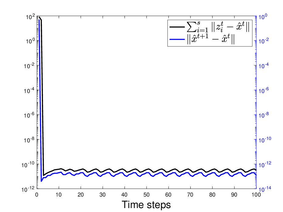
Fig. 1 (left) plots the $\log\det(P)$ and the center of the bounding ellipsoid of set ${\mathcal{T}}$ obtained by solving problem (31) via Algorithm 3 for the different number of samples $s$. A total of 50 Monte Carlo runs are simulated. It shows that the logdet and the center can quickly converge to a stable value as the number of samples $s$ increases. Therefore, Algorithm 3 can get stable estimation ellipsoids with a small number of samples. Furthermore, $\sum^{s}_{i=1}\|z_{i}^{t}-\hat{x}^{t}\|$ and $\|\hat{x}^{t+1}-\hat{x}^{t}\|$ versus the number of iterations $t$ for one random problem instance with $s=100$ are plotted in Fig. 1 (right). It shows that the differences between $z_{i}^{t}$ and $\hat{x}^{t}$, $\hat{x}^{t}$ and $\hat{x}^{t+1}$ rapidly decrease as the number of the algorithm iterations increases, i.e., (20)-(21) are satisfied indeed. In addition, the partial stopping criterion (the successive difference of $\hat{x}$ is smaller than a given tolerance) is also satisfied as the number of the iterations increases.

Consider the optimization problem (13) with a linear constraint ($g$ is a linear function), which can be rewritten by Schur complement [57]:

where $g(\hat{x})=C\hat{x}-c$. The solution of the linear estimation constraint is $\hat{x}=C^{\dagger}c+U\gamma$, where $U=I-C^{\dagger}C$ is an orthogonal projection matrix in $\mathcal{N}(C)$ and $\gamma\in\mathbb{R}^{n}$ is arbitrary. Then the problem (32) can be rewritten as an SDP problem by defining $H=P^{-1}$ and $\delta=P^{-1}U\gamma$:

In the problem (33), the dimension of decision variables is $M=\frac{n(n+1)}{2}+n$ and the dimension of the constraint matrix is $N=s(n+1)$. By using a primal-dual interior-point method to solve (33), the worst-case estimate requires $O(M^{2.75}s^{1.5})$ arithmetic operations to solve the problem with a given accuracy [58, 59]. Nevertheless, the consensus-ADMM method requires $O(n^{3}+sn^{2})$ arithmetic operations to solve the problem (13) with a linear constraint. Specific solution steps and corresponding computational complexity are as follows:

• •

  Update of $P$: Algorithm 2 is used to obtain the updated $\mu^{*}$. Each iteration of Algorithm 2 requires $O(n^{2}+(n+1)s)$ arithmetic operations, and calculating $P^{*}$ by equation (24) requires $O(sn^{2})$ arithmetic operations.

• •

  Update of $z_{i}$: The arithmetic operations is $O(n)$ for each $i$ at each iteration by caching the eigen-decomposition of $P$ and using Newton’s method to solve the equation $g(\phi_{i})=1$ [37]. The eigen-decomposition of $P$ requires $O(n^{3})$ arithmetic operations.

• •

  Update of $\hat{x}$: Calculating $\hat{x}^{*}$ by equation (30) requires $O(n^{3})$ arithmetic operations.

Therefore, consensus-ADMM method requires $O(n^{3}+sn^{2})$ arithmetic operations to solve the problem (13) with a linear constraint, which is much lower than $O(M^{2.75}s^{1.5})$ arithmetic operations of the SDP method.

For the problem (13) with a quadratic constraint, by similar analysis and using the Newton’s method to calculate the updated $\hat{x}^{*}$, the consensus-ADMM method also requires $O(n^{3}+sn^{2})$ arithmetic operations to solve it. For the problem (13) with a general form constraint, the consensus-ADMM method requires $O(n^{3}+sn^{2})$ arithmetic operations together with the computation of the constraint function and its gradient to solve it since the computational complexity of updating $\hat{x}$ depends on the specific form of the constraint function, and it costs computation of the constraint function and its gradient together with $O(n^{3})$ arithmetic operations to obtain an updated $\hat{x}^{*}$ via a basic implementation of Newton’s method at each iteration [53]. Nevertheless, the SDP method is not suitable for solving the problem (13) with the nonlinear constraint.

In the following example, we compare the computing time for solving problem (32) by using SDPT3 [60] and the consensus-ADMM algorithm, respectively.

Example 2. Suppose there are $s$ samples $r_{i}\in\mathbb{R}^{\hat{n}}$ that are generated by a random generate ellipsoid $\mathcal{E}(0,\hat{P})$. $C=[\hat{C},-1,0,...,0]\in\mathbb{R}^{1\times\hat{n}}$, $c=0$, and $\hat{C}$ is generated by the standard uniform distribution. The computing time of different methods for solving problem (32) is given in Table 1. SDP indicates that the SDP problem (33) is solved by SDPT3, C(S)-ADMM indicates sequential computation at the update of $z_{i}$ when solving the problem (32) with the consensus-ADMM algorithm, and C(P)-ADMM indicates parallel computation at the update of $z_{i}$ when solving the problem (32) with the consensus-ADMM algorithm. The results show that the consensus-ADMM algorithm takes less computing time than the SDP method. It is consistent with their computational complexity as $O(n^{3}+sn^{2})$ and $O((\frac{n(n+1)}{2}+n)^{2.75}s^{1.5})$, respectively. In this example, the computation times of the consensus-ADMM algorithms are on the order of 0.1$\sim$1 sec. The alternative approach to further reduce the computation time of the proposed consensus-ADMM algorithm is using the hardware acceleration methods or selecting specific subproblem solvers according to the structure of the optimization problems.

In this example, we consider the problem of tracking a target in two dimensions, and the dynamic system is given by:

where $x_{k}:=(s^{x}_{k},s^{y}_{k},\sigma^{x}_{k},\sigma^{y}_{k})$ and $T=1$ is the sampling time. The noises are assumed to be restricted in $w_{k}\in{\mathcal{E}}(0,Q_{k})$ and $v_{k}\in{\mathcal{E}}(0,R_{k})$, respectively, where $Q_{k}=10I_{4\times 4}$ and $R_{k}=diag(20^{2},0.1^{2})$. The estimation constraint on the above system is $C\hat{x}_{k}=c$, where $C=\begin{bmatrix}2&-1&0&0\\ 0&0&2&-1\end{bmatrix}$ and $c=[0,0]^{T}$.

References

- [1] Sajad Saeedi, Michael Trentini, Mae Seto, and Howard Li. Multiple-robot simultaneous localization and mapping: A review. Journal of Field Robotics, 33(1):3–46, 2016.
- [2] Jian Lan and X. Rong Li. Multiple conversions of measurements for nonlinear estimation. IEEE Transactions on Signal Processing, 65(18):4956–4970, 2017.
- [3] Sandy Mahfouz, Farah Mourad-Chehade, Paul Honeine, Joumana Farah, and Hichem Snoussi. Target tracking using machine learning and Kalman filter in wireless sensor networks. IEEE Sensors Journal, 14(10):3715–3725, 2014.
- [4] Dan Simon and Donald L Simon. Kalman filtering with inequality constraints for turbofan engine health estimation. IEE Proceedings-Control Theory and Applications, 153(3):371–378, 2006.
- [5] Ali T Alouani and William D Blair. Use of a kinematic constraint in tracking constant speed, maneuvering targets. IEEE Transactions on Automatic Control, 38(7):1107–1111, 1993.
- [6] Rudolph Emil Kalman. A new approach to linear filtering and prediction problems. Journal of Basic Engineering, 82(1):35–45, 1960.
- [7] Zhe Chen. Bayesian filtering: From Kalman filters to particle filters, and beyond. Statistics, 182(1):1–69, 2003.
- [8] Dan Simon. Kalman filtering with state constraints: A survey of linear and nonlinear algorithms. IET Control Theory & Applications, 4(8):1303–1318, 2010.
- [9] Branko Ristic, Sanjeev Arulampalam, and Neil Gordon. Beyond the Kalman filter: Particle filters for tracking applications. Artech house, 2003.
- [10] Yunmin Zhu. Multisensor decision and estimation fusion. Kluwer Academic Publishers, 2003.
- [11] Boris T Polyak, Sergey A Nazin, CéCile Durieu, and Eric Walter. Ellipsoidal parameter or state estimation under model uncertainty. Automatica, 40(7):1171–1179, 2004.
- [12] Fred Schweppe. Recursive state estimation: Unknown but bounded errors and system inputs. IEEE Transactions on Automatic Control, 13(1):22–28, 1968.
- [13] Laurent El Ghaoui and Giuseppe Calafiore. Robust filtering for discrete-time systems with bounded noise and parametric uncertainty. IEEE Transactions on Automatic Control, 46(7):1084–1089, 2001.
- [14] Xiaojing Shen, Yunmin Zhu, Enbin Song, and Yingting Luo. Minimizing Euclidian state estimation error for linear uncertain dynamic systems based on multisensor and multi-algorithm fusion. IEEE Transactions on Information Theory, 57(10):7131–7146, 2011.
- [15] Zhiguo Wang, Xiaojing Shen, and Yunmin Zhu. Ellipsoidal fusion estimation for multisensor dynamic systems with bounded noises. IEEE Transactions on Automatic Control, 64(11):4725–4732, Nov 2019.
- [16] Zhiguo Wang, Xiaojing Shen, Haiqi Liu, Fanqin Meng, and Yunmin Zhu. Dual set membership filter with minimizing nonlinear transformation of ellipsoid. IEEE Transactions on Automatic Control, 67(5):2405–2418, 2022.
- [17] Cécile Durieu, E Walter, and Boris Polyak. Multi-input multi-output ellipsoidal state bounding. Journal of optimization theory and applications, 111(2):273–303, 2001.
- [18] Yuan Wang, Jian Huang, Dongrui Wu, Zhi-Hong Guan, and Yan-Wu Wang. Set-membership filtering with incomplete observations. Information Sciences, 517:37–51, 2020.
- [19] Bo Chen and Guoqiang Hu. Nonlinear state estimation under bounded noises. Automatica, 98:159–168, 2018.
- [20] Brenner S Rego, Joseph K Scott, Davide M Raimondo, and Guilherme V Raffo. Set-valued state estimation of nonlinear discrete-time systems with nonlinear invariants based on constrained zonotopes. Automatica, 129:109638, 2021.
- [21] Eelco Scholte and Mark E Campbell. A nonlinear set-membership filter for on-line applications. International Journal of Robust and Nonlinear Control: IFAC-Affiliated Journal, 13(15):1337–1358, 2003.
- [22] Giuseppe Calafiore. Reliable localization using set-valued nonlinear filters. IEEE Transactions on systems, man, and cybernetics-part A: systems and humans, 35(2):189–197, 2005.
- [23] Shangkun Xiong, Fangjiong Chen, and Gang Wei. Blind multiuser detection based on linear constrained MMSE. In 2003 IEEE International Conference on Acoustics, Speech, and Signal Processing, 2003. Proceedings.(ICASSP’03)., volume 4, pages IV–445. IEEE, 2003.
- [24] Jie Zhou and Yunmin Zhu. The linear minimum mean-square error estimation with constraints and its applications. In 2006 International Conference on Computational Intelligence and Security, volume 2, pages 1801–1804. IEEE, 2006.
- [25] Zhansheng Duan and X Rong Li. Modeling of target motion constrained on straight line. IEEE Transactions on Aerospace and Electronic Systems, 52(2):548–562, 2016.
- [26] Thia Kirubarajan, Yaakov Bar-Shalom, Krishna R Pattipati, and Ivan Kadar. Ground target tracking with variable structure IMM estimator. IEEE Transactions on Aerospace and Electronic Systems, 36(1):26–46, 2000.
- [27] Fuwen Yang and Yongmin Li. Set-membership filtering for discrete-time systems with nonlinear equality constraints. IEEE Transactions on Automatic Control, 54(10):2480–2486, 2009.
- [28] Fuwen Yang and Yongmin Li. Set-membership filtering with state constraints. IEEE Transactions on Aerospace and Electronic Systems, 45(4):1619–1629, 2009.
- [29] Xiaowei Li, Xuedong Yuan, Fanqin Meng, Yiwei Liao, Haiqi Liuc, Xuqi Zhang, and Xiaojing Shen. Set-membership filtering for nonlinear dynamic systems with quadratic inequality constraints. IEEE Access, 8:13375–13386, 2020.
- [30] David Avis, David Bremner, and Raimund Seidel. How good are convex hull algorithms? Computational Geometry, 7(5-6):265–301, 1997.
- [31] Xiang Li, Wenhai Wang, Lijun Wu, Shuo Chen, Xiaolin Hu, Jun Li, Jinhui Tang, and Jian Yang. Generalized focal loss: Learning qualified and distributed bounding boxes for dense object detection. Advances in Neural Information Processing Systems, 33:21002–21012, 2020.
- [32] Antoine Girard. Reachability of uncertain linear systems using zonotopes. In International Workshop on Hybrid Systems: Computation and Control, pages 291–305. Springer, 2005.
- [33] EK Kostousova. Control synthesis via parallelotopes: optimzation and parallel compuations. Optimization methods and software, 14(4):267–310, 2001.
- [34] Olaf Stursberg and Bruce H Krogh. Efficient representation and computation of reachable sets for hybrid systems. In International Workshop on Hybrid Systems: Computation and Control, pages 482–497. Springer, 2003.
- [35] Alex A Kurzhanskiy and Pravin Varaiya. Ellipsoidal techniques for reachability analysis of discrete-time linear systems. IEEE Transactions on Automatic Control, 52(1):26–38, 2007.
- [36] Stephen Boyd, Neal Parikh, and Eric Chu. Distributed optimization and statistical learning via the alternating direction method of multipliers. Now Publishers Inc, 2011.
- [37] Kejun Huang and Nicholas D Sidiropoulos. Consensus-ADMM for general quadratically constrained quadratic programming. IEEE Transactions on Signal Processing, 64(20):5297–5310, 2016.
- [38] Wenqiang Pu, Ya-Feng Liu, Junkun Yan, Hongwei Liu, and Zhi-Quan Luo. Optimal estimation of sensor biases for asynchronous multi-sensor data fusion. Mathematical Programming, 170(1):357–386, 2018.
- [39] Simon J Julier and Jeffrey K Uhlmann. Unscented filtering and nonlinear estimation. Proceedings of the IEEE, 92(3):401–422, 2004.
- [40] Sebastian Thrun. Probabilistic robotics. Communications of the ACM, 45(3):52–57, 2002.
- [41] Laurent El Ghaoui and Giuseppe Calafiore. Worst-case simulation of uncertain systems. In Robustness in identification and control, pages 134–146. Springer, 1999.
- [42] Aharon Ben-Tal and Arkadi Nemirovski. On tractable approximations of uncertain linear matrix inequalities affected by interval uncertainty. SIAM Journal on Optimization, 12(3):811–833, 2002.
- [43] Sissi Xiaoxiao Wu, Man-Chung Yue, Anthony Man-Cho So, and Wing-Kin Ma. SDR approximation bounds for the robust multicast beamforming problem with interference temperature constraints. In 2017 IEEE International Conference on Acoustics, Speech and Signal Processing (ICASSP), pages 4054–4058. IEEE, 2017.
- [44] Rainer Hettich. An implementation of a discretization method for semi-infinite programming. Mathematical Programming, 34(3):354–361, 1986.
- [45] Rembert Reemtsen and Jan-J Rückmann. Semi-infinite programming, volume 25. Springer Science & Business Media, 1998.
- [46] Elijah Polak and Limin He. Rate-preserving discretization strategies for semi-infinite programming and optimal control. SIAM journal on control and optimization, 30(3):548–572, 1992.
- [47] Marco López and Georg Still. Semi-infinite programming. European journal of operational research, 180(2):491–518, 2007.
- [48] Ya-Feng Liu, Mingyi Hong, and Enbin Song. Sample approximation-based deflation approaches for chance SINR-constrained joint power and admission control. IEEE Transactions on Wireless Communications, 15(7):4535–4547, 2016.
- [49] Giuseppe Calafiore and Marco C Campi. Uncertain convex programs: randomized solutions and confidence levels. Mathematical Programming, 102(1):25–46, 2005.
- [50] Nima Rabiei and Elias G Saleeby. On intersection volumes of confidence hyper-ellipsoids and two geometric Monte Carlo methods. Monte Carlo Methods and Applications, 27(2):153–167, 2021.
- [51] Jonathan Eckstein and Dimitri P Bertsekas. On the Douglas—Rachford splitting method and the proximal point algorithm for maximal monotone operators. Mathematical Programming, 55(1):293–318, 1992.
- [52] Yangyang Xu, Wotao Yin, Zaiwen Wen, and Yin Zhang. An alternating direction algorithm for matrix completion with nonnegative factors. Frontiers of Mathematics in China, 7(2):365–384, 2012.
- [53] Dimitri P Bertsekas. Nonlinear programming. Journal of the Operational Research Society, 48(3):334–334, 1997.
- [54] Michael J Todd. Minimum-volume ellipsoids: Theory and algorithms. SIAM, 2016.
- [55] S Damla Ahipasaoglu, Peng Sun, and Michael J Todd. Linear convergence of a modified Frank–Wolfe algorithm for computing minimum-volume enclosing ellipsoids. Optimisation Methods and Software, 23(1):5–19, 2008.
- [56] S Damla Ahipaşaoğlu and Michael J Todd. A modified Frank–Wolfe algorithm for computing minimum-area enclosing ellipsoidal cylinders: Theory and algorithms. Computational Geometry, 46(5):494–519, 2013.
- [57] Stephen Boyd, Stephen P Boyd, and Lieven Vandenberghe. Convex optimization. Cambridge university press, 2004.
- [58] Lieven Vandenberghe and Stephen Boyd. Semidefinite programming. SIAM review, 38(1):49–95, 1996.
- [59] Stephen Boyd, Laurent El Ghaoui, Eric Feron, and Venkataramanan Balakrishnan. Linear matrix inequalities in system and control theory, volume 15. SIAM, 1994.
- [60] Michael Grant and Stephen Boyd. CVX: Matlab software for disciplined convex programming, version 2.1, March 2014.
Appendix A The proof of Lemma 1
Appendix B The proof of Theorem 1
Proof: Define , then (13) can be rewritten as: