UCI-TR-2022-24 DESY-22-171 A minimal modular invariant neutrino model

The origin of hierarchical fermion masses and flavor mixing parameters is a long-standing puzzle of particle physics, and flavor symmetry has been extensively studied as a guiding principle to understand the flavor puzzle, see Refs. [1, 2, 3, 4] for review on this topic. The modular invariance as flavor symmetry was recently proposed to provide a promising framework to address the flavor structure of SM. The Yukawa couplings are constrained to be modular forms of level $N$ which are holomorphic functions of the complex modulus $\tau$, and the flavor symmetry could be uniquely broken down by the vacuum expectation value of $\tau$. The modular flavor symmetry allows to construct predictive flavor models characterized by a small number of Lagrangian parameters, and it is remarkable that all higher-dimensional operators in the superpotential are unambiguously determined in the limit of unbroken supersymmetry (SUSY).

The model construction is based the inhomogeneous finite modular groups $\Gamma_{N}\equiv\bar{\Gamma}/\bar{\Gamma}(N)$ [5] or homogeneous finite modular groups $\Gamma^{\prime}_{N}\equiv\Gamma/\Gamma(N)$ [6]. For finite modular groups of small order, many lepton and quark mass models have been constructed and discussed, for example $\Gamma_{2}\cong S_{3}$ [7, 8], $\Gamma_{3}\cong A_{4}$ [5, 9, 7, 10, 11, 8, 12, 13, 14, 15, 16, 17, 18, 19, 20, 21, 22, 23, 24, 25, 26, 27], $\Gamma_{4}\cong S_{4}$ [28, 29, 30, 31, 32, 33, 34, 16, 35, 36], $\Gamma_{5}\cong A_{5}$ [37, 38, 33], $\Gamma_{7}\cong\mathrm{PSL}(2,\mathbb{Z}_{7})$ [39], $\Gamma^{\prime}_{3}\cong T^{\prime}$ [6, 40, 41], $\Gamma^{\prime}_{4}\cong S^{\prime}_{4}$ [42, 43], $\Gamma^{\prime}_{5}\cong A^{\prime}_{5}$ [44, 45, 46] and $\Gamma^{\prime}_{6}\cong S_{3}\times T^{\prime}$ [47]. In the modular invariant models, the Yukawa couplings are integer weight modular forms of the principal congruence subgroup $\Gamma(N)$. Recently, $\Gamma_{N}$ and $\Gamma^{\prime}_{N}$ has been extended to the most general finite modular groups [48], where the modular forms of $N$ are generalized to be the vector valued modular forms of $\mathrm{SL}(2,\mathbb{Z})$. Moreover, the rational weight modular form in modular flavor symmetry and the metaplectic finite modular groups $\widetilde{\Gamma}_{N}\equiv\widetilde{\Gamma}/\widetilde{\Gamma}(N)$ are discussed in Refs. [49, 45]. It is known that there are only three independent fixed points $\tau=i$, $e^{2\pi i/3}$, $i\infty$ in the fundamental domain of the modular group [16]. It has been recognized that the mass hierarchies of the charged leptons can arise from the deviation of the complex modulus from these fixed points [50, 51, 52, 53]. In the top-down approach such as string theory, generally multiple moduli are involved. In view of this, the $\mathrm{SL}(2,\mathbb{Z})$ modular symmetry with single complex modulus has been extended to the $\mathrm{Sp}(2g,\mathbb{Z})$ symplectic modular symmetry and even other modular symmetries in higher dimensional moduli space [54], where the classical modular forms are replaced by more general automorphic forms. The symplectic modular symmetry would be reduced to the product of several $\mathrm{SL}(2,\mathbb{Z})$ with certain mirror symmetry [30, 32] when the moduli space is factorized into several independent tori. The predictive power of modular symmetry can be further improved by including the generalized CP symmetry. It is found that the generalized CP symmetry can be consistently combined with symplectic modular symmetries for both single modulus with $g=1$ [55, 56, 57] and multiple moduli with $g\geq 2$ [58]. The generalized CP symmetry can enforce the coupling constants to be real in certain representation basis, so that the vacuum expectation value (VEV) of $\tau$ is the unique source of flavor symmetry breaking and CP violation. The modular symmetry also can be embed into $\mathrm{SU}(5)$ and $\mathrm{SO}(10)$ Grand Unified Theories [59, 60, 61, 62, 63, 64, 65, 66, 67]. Furthermore, the modular symmetry can naturally appears in top-down constructions [56, 68, 69, 70, 71, 72, 73, 74, 75, 76]. However, it is found that the modular symmetry is usually accompanied by traditional flavor symmetry, this scheme is named as eclectic flavor group [77, 78, 79, 80, 81]. Some models based on eclectic flavor symmetry have been proposed [25, 82].

The modular flavor symmetry is attractive because the modular invariant mass models usually contain only a few free input parameters, so they have a certain predictive power. Therefore, it is of great significance to find a realistic model with the least free parameters in this framework. As far as we know, the modular invariant models in the literature require at least 7 parameters to explain 12 observables in the lepton sector alone [55, 43, 22, 36], and at least 9 parameters to explain 10 observables in the quark sector alone [43, 22, 36]. In this paper, after searching a large number of possible models, we succeeded in finding a modular invariant lepton model with the fewest parameters so far, which contains only 6 real free parameters but successfully matches the current experimental data. We carefully analyze the best-fit values of this model and perform an exhaustive scan of the parameter space, we find interesting features of the neutrino mixing angles and CP violation phases predicted by this model. On the other hand, the modular invariant supersymmetry theory constrains not only the flavor structures of quarks and leptons, but also the flavor structures of their superpartners, which leads to specific patterns in soft SUSY breaking terms [61, 83]. These terms will cause lepton flavor violation at low energy. Therefore, we also study the soft SUSY breaking terms in our minimal lepton model and their flavor phenomenological implications such as the branching ratio of rare decay $\mu\to e\gamma$.

This paper is organized as follows. In section 2, the modular symmetry and the soft SUSY breaking terms in modular invariant supergravity are reviewed. In section 3, we present the minimal lepton model which is based on finite modular group $S^{\prime}_{4}$, and also analyze the predictions of this model numerically. In section 4, we show the soft breaking terms in our minimal model, and calculate the branch ratio of lepton flavor violation process $\mu\rightarrow e\gamma$. The finite modular groups $\Gamma^{\prime}_{4}\cong S^{\prime}_{4}$ and its Clebsch-Gordan coefficients are given in Appendix A. In Appendix B, we give the explicit expressions of the relevant modular forms.

We restrict ourselves to the framework of modular invariant supergravity with single modulus [84, 5], and consider the moduli-mediated SUSY breaking [85, 86, 87, 88]. The modular symmetry are characterized by the modular group $\Gamma\equiv\mathrm{SL}(2,\mathbb{Z})$ which consists of matrices with integer entries:

$$\mathrm{SL}(2,\mathbb{Z})=\left\{\begin{pmatrix}a&~b\\ c&~d\end{pmatrix}\Big|~ad-bc=1\,,\quad a,b,c,d\in\mathbb{Z}\,\right\}\,.$$

(1)

It can be generated by two generators $S$ and $T$

$$S=\begin{pmatrix}0&~1\\ -1&~0\end{pmatrix}\,,\qquad T=\begin{pmatrix}1&~1\\ 0&~1\end{pmatrix}\,.$$

(2)

They obey the following relations

$$S^{4}=(ST)^{3}=1\,,\quad S^{2}T=TS^{2}\,.$$

(3)

Note that $S^{2}=-\mathbb{1}_{2}$, where $\mathbb{1}_{2}$ denotes the two-dimensional identity matrix. The modular group $\Gamma$ acts on the complex upper half-plane $\mathcal{H}=\{\tau\in\mathbb{C}~|~\text{Im}\tau>0\}$ by linear fractional transformation

$$\gamma\tau\equiv\frac{a\tau+b}{c\tau+d}\,,\qquad\gamma=\begin{pmatrix}a&b\\ c&d\end{pmatrix}\in\Gamma\,.$$

(4)

It is easy to find that $\gamma$ and $-\gamma$ give the same action on $\tau$ and thus the faithful action of the linear fractional transformation is given by the projective special linear group $\mathrm{PSL}(2,\mathbb{Z})$ which is the quotient group $\mathrm{PSL}(2,\mathbb{Z})\cong\mathrm{SL}(2,\mathbb{Z})/\{\pm\mathbb{1}_{2}\}$.

The action of modular group on the matter fields $\Phi_{i}$ is assumed as follows

$$\Phi_{i}\stackrel{{\scriptstyle\gamma}}{{\longrightarrow}}(c\tau+d)^{-k_{i}}\rho(\gamma)\Phi_{i}\,,$$

(5)

where $-k_{i}$ is called the modular weight of matter field $\Phi_{i}$, and $\rho(\gamma)$ is the unitary irreducible representation of $\mathrm{SL}(2,\mathbb{Z})$ with finite image [48]. In general, the representation can be taken for cases where its kernels are principal congruence subgroups $\Gamma(N)$, and the $\rho(\gamma)$ is often referred to as the representation of finite modular groups $\Gamma^{\prime}_{N}\equiv\Gamma/\Gamma(N)$.

The full $\mathcal{N}=1$ supergravity Lagrangian is specified in terms of two functions: the gauge kinetic function $f_{a}$ and the real gauge-invariant Kähler function $\mathcal{G}(\tau,\Phi_{i};\bar{\tau},\bar{\Phi}_{i})$ ¹¹ 1 We use the standard supergravity mass units, namely the reduced Planck mass $M_{p}\equiv M_{Planck}/\sqrt{8\pi}=1$.. $f_{a}$ determines the kinetic terms for the fields in the vector multiplets and in particular the gauge coupling constant, $\text{Re}f_{a}=1/g^{2}_{a}$, where the subscript $a$ is associated with the different gauge groups of the theory. The Kähler function is the combination [85, 88]:

$$\mathcal{G}(\tau,\Phi_{i};\bar{\tau},\bar{\Phi}_{i})=\mathcal{K}(\tau,\Phi_{i};\bar{\tau},\bar{\Phi}_{i})+\log\mathcal{W}(\tau,\Phi_{i})+\log\mathcal{\overline{W}}(\bar{\tau},\bar{\Phi}_{i})\,,$$

(6)

where the Kähler potential and superpotential have the form

	$\displaystyle\mathcal{K}$	$\displaystyle=\mathcal{K}_{\tau}+\mathcal{K}_{matter}+\dots\,,$		(7)
	$\displaystyle\mathcal{W}$	$\displaystyle=Y_{ijk}(\tau)\Phi^{i}\Phi^{j}\Phi^{k}+\mu_{ij}(\tau)\Phi^{i}\Phi^{j}+\dots\,.$		(8)

In particular, we take the minimal form of Kähler potential [5]

$$\mathcal{K}_{\tau}=-\log(-i(\tau-\bar{\tau}))\,,\quad\mathcal{K}_{matter}=\tilde{\mathcal{K}}_{i\bar{i}}|\Phi^{i}|^{2}=(-i(\tau-\bar{\tau}))^{-k_{i}}|\Phi^{i}|^{2}\,,$$

(9)

where $\tilde{\mathcal{K}}_{i\bar{i}}$ is the Kähler metric. As you can see, the transformation of the Kähler potential induced by the modular transformation of fields is exactly a Kähler transformation:

$$\mathcal{K}\stackrel{{\scriptstyle\gamma}}{{\longrightarrow}}\mathcal{K}+\log(c\tau+d)+\log(c\bar{\tau}+d)\,.$$

(10)

Hence, the modular invariance of Kähler function $\mathcal{G}$ requires that the superpotential must be transformed complementally:

$$\mathcal{W}\stackrel{{\scriptstyle\gamma}}{{\longrightarrow}}(c\tau+d)^{-1}\mathcal{W}\,.$$

(11)

In other words, the superpotential behaves like a chiral superfield with modular weight $-1$. Modular invariance requires that the Yukawa couplings $Y_{ijk}(\tau)$ in Eq. (8) should be modular forms of weight $k_{Y}$, specifically,

$$Y_{ijk}(\tau)\stackrel{{\scriptstyle\gamma}}{{\longrightarrow}}Y_{ijk}(\gamma\tau)=(c\tau+d)^{k_{Y}}\rho(\gamma)_{(ijk)(lmn)}Y_{lmn}(\tau)$$

(12)

with $k_{Y}=k_{i}+k_{j}+k_{k}-1$ and product $\rho\times\rho_{i}\times\rho_{j}\times\rho_{k}$ contains an invariant singlet.

The scalar component of modulus in the hidden sector, $\tau$, may obtain large VEV that induce SUSY breaking via non-vanishing VEV of its auxiliary field $F^{\tau}$. The gravition becomes massive and its mass is given by [85, 88]

$$m_{3/2}=e^{\mathcal{G}/2}M_{p}\,.$$

(13)

On the other hand, after taking the so-called flat limit where $M_{p}\to\infty$ but $m_{3/2}$ is kept fixed, all that is left in the observable sector is a effective global SUSY Lagrangian plus a set of soft SUSY-breaking terms. The effective superpotential is given by  [85, 88]

$$\mathcal{W}^{(eff)}(\Phi_{i})=\hat{Y}_{ijk}(\tau)\hat{\Phi}^{i}\hat{\Phi}^{j}\hat{\Phi}^{k}+\hat{\mu}_{ij}(\tau)\hat{\Phi}^{i}\hat{\Phi}^{j}$$

(14)

in the canonically normalized basis, with normalized Yukawa couplings and normalized masses

$$\hat{Y}_{ijk}=Y_{ijk}e^{\mathcal{K}_{\tau}/2}\left(\tilde{\mathcal{K}}_{i\bar{i}}\tilde{\mathcal{K}}_{j\bar{j}}\tilde{\mathcal{K}}_{k\bar{k}}\right)^{-1/2}\,,\quad\hat{\mu}_{ij}=\mu_{ij}e^{\mathcal{K}_{\tau}/2}\left(\tilde{\mathcal{K}}_{i\bar{i}}\tilde{\mathcal{K}}_{j\bar{j}}\right)^{-1/2}\,.$$

(15)

The effective soft SUSY-breaking Lagrangian in the canonically normalized basis is given by [85, 88]

$$\mathcal{L}_{soft}=\frac{1}{2}\left(M_{a}\hat{\lambda}^{a}\hat{\lambda}^{a}+\mathrm{h.c.}\right)-\tilde{m}^{2}_{i}\bar{\hat{\Phi}}^{i}\hat{\Phi}^{i}-\left(A_{ijk}\hat{Y}_{ijk}\hat{\Phi}^{i}\hat{\Phi}^{j}\hat{\Phi}^{k}+B\hat{\mu}\hat{H}_{u}\hat{H}_{d}+\mathrm{h.c.}\right)$$

(16)

with

	$\displaystyle\tilde{m}_{i}^{2}$	$\displaystyle=m_{3/2}^{2}-|F^{\tau}|^{2}\partial_{\bar{\tau}}\partial_{\tau}\log\tilde{\mathcal{K}}_{i\bar{i}}\,,$		(17)
	$\displaystyle M_{a}$	$\displaystyle=\frac{1}{2}\left(\mathrm{Re}f_{a}\right)^{-1}F^{\tau}\partial_{\tau}f_{a}\,,$
	$\displaystyle A_{ijk}$	$\displaystyle=F^{\tau}\left[\partial_{\tau}\mathcal{K}_{\tau}+\partial_{\tau}\log Y_{ijk}-\partial_{\tau}\log\left(\tilde{\mathcal{K}}_{i\bar{i}}\tilde{\mathcal{K}}_{j\bar{j}}\tilde{\mathcal{K}}_{k\bar{k}}\right)\right]\,,$
	$\displaystyle B$	$\displaystyle=F^{\tau}\left[\partial_{\tau}\mathcal{K}_{\tau}+\partial_{\tau}\log\mu-\partial_{\tau}\log\left(\tilde{\mathcal{K}}_{H_{u}}\tilde{\mathcal{K}}_{H_{d}}\right)\right]-m_{3/2}\,,$

where $\tilde{\mathcal{K}}_{H_{u,d}}=(-i(\tau-\bar{\tau}))^{-k_{H_{u,d}}}$, $\hat{\Phi}^{i}$ and $\hat{\lambda}^{a}$ are the scalar and gaugino canonically normalized fields respectively

$$\hat{\Phi}^{i}=\tilde{\mathcal{K}}_{i\bar{i}}^{1/2}\Phi^{i}\,,\quad\hat{\lambda}^{a}=(\mathrm{Re}f_{a})^{1/2}\lambda^{a}\,.$$

(18)

In this section, we shall present a model for neutrino masses and mixing based on the $S^{\prime}_{4}$ modular symmetry, and it depends on only six real parameters including the modulus $\tau$. It is the phenomenologically viable lepton mass model with the smallest number of free parameters as far as we know. The generalized CP (gCP) symmetry has been included in this model in order to increase the predictive power. It is known the complex modulus $\tau$ transforms as $\tau\rightarrow-\tau^{*}$ under the action of gCP. In the symmetric basis where both modular generator $S$ and $T$ are represented by symmetric and unitary matrices, gCP reduces to canonical CP transformation [55, 58]. As a consequence, the gCP symmetry would constrain all couplings constants to be real in the representation basis with real Clebsch-Gordan coefficients. As shown in the Appendix A, we indeed works in symmetric basis of $S^{\prime}_{4}$ and the all the Clebsch-Gordan coefficients are real.

In this model, the neutrino masses are described by type-I seesaw mechanism. We introduce three right-handed neutrinos $N^{c}=(N^{c}_{1},N^{c}_{2},N^{c}_{3})^{T}$ and assume that they transform according to the triplet $\mathbf{3}$ of $S^{\prime}_{4}$. In charged lepton sector, the first two generations of the right-handed charged leptons $E^{c}_{D}=(E^{c}_{1},E^{c}_{2})^{T}$ are assigned to the doublet representation $\mathbf{\hat{2}}$, and the third generation of the right-handed charged leptons $E^{c}_{3}$ is assigned to be $S^{\prime}_{4}$ singlet. The left-handed charged lepton $L=(L_{1},L_{2},L_{3})^{T}$ transforms as a triplet $\mathbf{3}$. The representation and weight assignments of the fields are summarized as follows:

		$\displaystyle\rho_{E^{c}}=\mathbf{\hat{2}}\oplus\mathbf{\hat{1}^{\prime}},~\quad\rho_{L}=\mathbf{3},\quad~\rho_{N^{c}}=\mathbf{3},~\quad\rho_{H_{u}}=\rho_{H_{d}}=\mathbf{1}\,,$
		$\displaystyle k_{E_{1,2,3}^{c}}=11/2,11/2,11/2\,,~\quad k_{N^{c}}=3/2,~\quad k_{L}=-3/2\,,~\quad k_{H_{u}}=k_{H_{d}}=0\,.$		(19)

The superpotential of the lepton sector includes:

	$\displaystyle\mathcal{W}_{e}$	$\displaystyle=\alpha\left(E_{D}^{c}LY^{(3)}_{\mathbf{\hat{3}^{\prime}}}\right)_{\mathbf{1}}H_{d}+\beta\left(E_{D}^{c}LY^{(3)}_{\mathbf{\hat{3}}}\right)_{\mathbf{1}}H_{d}+\gamma\left(E_{3}^{c}LY^{(3)}_{\mathbf{\hat{3}}}\right)_{\mathbf{1}}H_{d}\,,$
	$\displaystyle\mathcal{W}_{\nu}$	$\displaystyle=g_{1}\left(N^{c}L\right)_{\mathbf{1}}H_{u}+\Lambda\left((N^{c}N^{c})_{\mathbf{2},s}Y^{(2)}_{\mathbf{2}}\right)_{\mathbf{1}}\,.$		(20)

Then, the charged lepton and neutrino mass matrices can be read off by using the Clebsch-Gordon coefficients of $S^{\prime}_{4}$ shown in Appendix A:

		$\displaystyle M_{e}=\begin{pmatrix}2\alpha Y^{(3)}_{\mathbf{\hat{3}^{\prime}},1}~&~-\alpha Y^{(3)}_{\mathbf{\hat{3}^{\prime}},3}+\sqrt{3}\beta Y^{(3)}_{\mathbf{\hat{3}},2}~&~-\alpha Y^{(3)}_{\mathbf{\hat{3}^{\prime}},2}+\sqrt{3}\beta Y^{(3)}_{\mathbf{\hat{3}},3}\\ -2\beta Y^{(3)}_{\mathbf{\hat{3}},1}~&~\sqrt{3}\alpha Y^{(3)}_{\mathbf{\hat{3}^{\prime}},2}+\beta Y^{(3)}_{\mathbf{\hat{3}},3}~&~\sqrt{3}\alpha Y^{(3)}_{\mathbf{\hat{3}^{\prime}},3}+\beta Y^{(3)}_{\mathbf{\hat{3}},2}\\ \gamma Y^{(3)}_{\mathbf{\hat{3}},1}~&~\gamma Y^{(3)}_{\mathbf{\hat{3}},3}~&~\gamma Y^{(3)}_{\mathbf{\hat{3}},2}\end{pmatrix}v_{d}\,,$
		$\displaystyle M_{D}=g\begin{pmatrix}1&0&0\\ 0&0&1\\ 0&1&0\end{pmatrix}v_{u}\,,\quad M_{N}=\Lambda\begin{pmatrix}2Y^{(2)}_{\mathbf{2},1}&0&0\\ 0&\sqrt{3}Y^{(2)}_{\mathbf{2},2}&-Y^{(2)}_{\mathbf{2},1}\\ 0&-Y^{(2)}_{\mathbf{2},1}&\sqrt{3}Y^{(2)}_{\mathbf{2},2}\end{pmatrix}\,.$		(21)

The light neutrino mass matrix $M_{\nu}$ is given by the seesaw formula

$$M_{\nu}=-M_{D}^{T}M_{N}^{-1}M_{D}=\frac{g^{2}v_{u}^{2}}{\Lambda}\begin{pmatrix}-\frac{1}{2Y^{(2)}_{\mathbf{2},1}}~&~0~&~0\\ 0~&~\frac{\sqrt{3}\;Y^{(2)}_{\mathbf{2},2}}{Y^{(2)2}_{\mathbf{2},1}-3Y^{(2)2}_{\mathbf{2},2}}~&~\frac{Y^{(2)}_{\mathbf{2},1}}{Y^{(2)2}_{\mathbf{2},1}-3Y^{(2)2}_{\mathbf{2},2}}\\ 0~&~\frac{Y^{(2)}_{\mathbf{2},1}}{Y^{(2)2}_{\mathbf{2},1}-3Y^{(2)2}_{\mathbf{2},2}}~&~\frac{\sqrt{3}\;Y^{(2)}_{\mathbf{2},2}}{Y^{(2)2}_{\mathbf{2},1}-3Y^{(2)2}_{\mathbf{2},2}}\end{pmatrix}\,.$$

(22)

It is remarkable that the light neutrino mass matrix $M_{\nu}$ is a block diagonal matrix, and consequently we can easily read off the light neutrino masses as follows:

$$m_{1}=\frac{1}{|2Y^{(2)}_{\mathbf{2},1}|}\frac{g^{2}v_{u}^{2}}{\Lambda}\,,\quad m_{2}=\frac{1}{|Y^{(2)}_{\mathbf{2},1}-\sqrt{3}Y^{(2)}_{\mathbf{2},2}|}\frac{g^{2}v_{u}^{2}}{\Lambda}\,,\quad m_{3}=\frac{1}{|Y^{(2)}_{\mathbf{2},1}+\sqrt{3}Y^{(2)}_{\mathbf{2},2}|}\frac{g^{2}v_{u}^{2}}{\Lambda}\,.$$

(23)

In the modular invariant models, the determinant of the lepton mass matrices are some one-dimensional vector-valued modular forms of $\mathrm{SL}(2,\mathbb{Z})$ [48]. In this minimal model, we have

$\displaystyle\det[M_{e}(\tau)]=-96\sqrt{6}v_{d}^{3}\gamma(\beta^{2}-3\alpha^{2})\eta^{18}(\tau)\,,$

(24)

where $\eta(\tau)=e^{\pi i\tau/12}\prod_{n=1}^{\infty}(1-e^{2\pi in\tau})$ is the well-known Dedekind eta function. We see that the small electron mass can be naturally reproduced for $\beta\approx\pm\sqrt{3}\alpha$.

As explained in the beginning of this section, the gCP symmetry constrains all couplings to be real in our working basis. Thus, all lepton flavor observable only depend on four coupling constants $\alpha$, $\beta$, $\gamma$, $g^{2}/\Lambda$ plus the complex modulus $\langle\tau\rangle$ in our model. A notable feature of this model is that the light neutrino mass matrix as well as the neutrino mass ratios are completely determined by the modulus $\tau$ up to the overall scale $g^{2}v^{2}_{u}/\Lambda$. After numerical fitting, we find the experimental data can be accommodated only if the neutrino masses are normal ordering, and the best-fit values of the input parameters that agree well with the experimental data are given by [89]:

$$\begin{gathered}\langle\tau\rangle=-0.193773+1.08321i\,,\quad\beta/\alpha=1.73048\,,\quad\gamma/\alpha=0.27031\,,\\ \alpha v_{d}=244.621~\text{MeV}\,,\quad g^{2}v^{2}_{u}/\Lambda=29.0744~\text{meV}\,,\end{gathered}$$

(25)

where $\alpha v_{d}$ and $g^{2}v^{2}_{u}/\Lambda$ are fixed by the measured values of the electron mass and the solar mass squared splitting $\Delta m^{2}_{21}$ respectively [89]. It is worth noting that all dimensionless input parameters happen to be $\mathcal{O}(1)$, and $\beta/\alpha$ is close to $\sqrt{3}$. Notice that the electron mass is exactly vanishing when $\beta/\alpha=\sqrt{3}$, see Eq. (24). At the above best fit point, the charged lepton mass ratios, the lepton mixing angles, CP violating phases and the neutrino masses are determined to be:

$$\begin{gathered}\sin^{2}\theta_{12}=0.328920\,,\quad\sin^{2}\theta_{13}=0.0218499\,,\quad\sin^{2}\theta_{23}=0.506956\,,\quad\delta_{CP}=1.34256\pi\,,\\ \alpha_{21}=1.32868\pi\,,~~\alpha_{31}=0.544383\pi\,,~~m_{e}/m_{\mu}=0.00472633,~~m_{\mu}/m_{\tau}=0.0587566\,,\\ m_{1}=14.4007~\text{meV}\,,\quad m_{2}=16.7803~\text{meV}\,,\quad m_{3}=51.7755~\text{meV}\,,\\ m_{\beta}=16.8907~\text{meV}\,,\quad m_{\beta\beta}=9.25333~\text{meV}\,,\end{gathered}$$

(26)

where $m_{\beta}$ is the effective neutrino masses probed by direct kinematic search in tritium beta decay and $m_{\beta\beta}$ is the effective mass in neutrinoless double beta decay. We see that the neutrino mass sum is predicted to be $m_{1}+m_{2}+m_{3}=82.9565$ meV which is compatible with the upper limit of Planck $\sum_{i}m_{i}<120$ meV [91]. We would like to emphasize that inverted neutrino mass ordering is disfavored in our model. The predicted neutrino mixing angles and CP violation phase $\delta_{CP}$ are within the $3\sigma$ intervals of the latest global fit NuFIT v5.1 without SK atmospheric data [89], the charged lepton mass ratios are compatible with their renormalization group (RG) running values at the GUT scale $2\times 10^{16}$ GeV, where $M_{\text{SUSY}}=1~\mathrm{TeV}\,,\tan\beta=5$ is taken as a benchmark [90].

From Eq. (23), we see that the light neutrino masses only depends on the VEV of the modulus $\tau$ and the overall mass scale $g^{2}v^{2}_{u}/\Lambda$. Hence we can use the measure value of the ratio $\Delta m^{2}_{21}/\Delta m^{2}_{31}$ to constrain the range of $\langle\tau\rangle$, where $\Delta m^{2}_{21}\equiv m^{2}_{2}-m^{2}_{1}$ and $\Delta m^{2}_{31}\equiv m^{2}_{3}-m^{2}_{1}$ are the solar and atmospheric neutrino mass squared differences respectively. The corresponding result is shown in the blue region of figure 1. Furthermore, we use the precisely measured values of the reactor angle $\theta_{13}$ and the charged lepton mass ratios $m_{e}/m_{\mu}$, $m_{\mu}/m_{\tau}$ to limit the phenomenologically allowed region of $\langle\tau\rangle$, and the both parameters $\beta/\alpha$ and $\gamma/\alpha$ are allowed to freely vary. The corresponding the result is displayed by the orange area in figure 1. Therefore the modulus should lie in two small regions around $-0.19+1.08i$ and $0.19+1.08i$ in order to accommodate the current data. Moreover, we also have comprehensively explored the parameter space of this minimal model. Requiring the three charged lepton masses $m_{e,\mu,\tau}$, the three lepton mixing angles $\theta_{12}$, $\theta_{13}$, $\theta_{23}$ and the neutrino squared mass splittings $\Delta m^{2}_{21}$ and $\Delta m^{2}_{31}$ to lie in the experimentally allowed $3\sigma$ regions [89], we get the correlations between the free parameters and observable quantities, which are shown in figure 2. If $\langle\tau\rangle$ is changed to $-\langle\tau\rangle^{*}$ and the values of coupling constants are kept intact, the sign of the CP violation phases $\delta_{CP}$, $\alpha_{21}$, $\alpha_{31}$ would be reversed while predictions for lepton masses and mixng angles remain the same. As a consequence, we only plot the region of $\text{Re}\langle\tau\rangle<0$ for simplicity. It can be seen that the overlapping region in figure 1 almost coincides with the $\langle\tau\rangle$ region shown in figure 2. It is remarkable that the phenomenologically viable parameter space is actually very small.

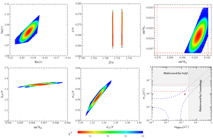
In particular, we notice that the neutrino mixing angle $\sin^{2}\theta_{23}$ is limited in the range of $0.504$ and $0.510$ which is in the second octant, the Dirac CP violation phase $\delta_{CP}$ lie in a very small interval $[1.316\pi,1.364\pi]$. These predictions for $\theta_{23}$ and $\delta_{CP}$ could be tested in forthcoming long baseline neutrino experiments DUNE [93] and T2HK [94]. In addition, the neutrino mixing angles $\sin^{2}\theta_{12}$ and $\sin^{2}\theta_{13}$ also show a certain correlation, this feature is expected to be tested at JUNO [95] which can measure the solar angle $\theta_{12}$ with sub-percent precision. Moreover, the Majorana CP violation phases are also found to lie in quite narrow regions $\alpha_{21}\in[1.309\pi,1.352\pi]$ and $\alpha_{31}\in[0.510\pi,0.576\pi]$. Consequently we have definite prediction for the effective Majorana mass $m_{\beta\beta}$ in the interval $[8.543~\text{meV},10.010~\text{meV}]$ which is within the reach of future ton-scale neutrinoless double beta decay experiments.

The SUSY flavor phenomena of lepton flavor violations (LFV) for lepton sector have been discussed in the traditional flavor symmetry models [96, 97, 98] and modular flavor models [83, 99]. In this section we will discuss the SUSY flavor phenomena in our minimal modular lepton model.

From the general results of the Kähler potential Eq. (9) and the soft terms Eq. (17), we can obtain the expressions of the soft mass and $A$-term coefficient as follow ²² 2 Interestingly, the soft mass $\tilde{m}_{i}^{2}$ is modular invariant because gravitino mass $m_{3/2}$ is modular invariant and $F^{\tau}$ has modular weight $-2$. The $A$-term $h_{ijk}\equiv Y_{ijk}A_{ijk}$ transform in the same way as $Y_{ijk}$ and they are the non-holomorphic modular forms of weight $k_{Y}$ [100].:

	$\displaystyle\tilde{m}_{i}^{2}$	$\displaystyle=m^{2}_{3/2}-k_{i}\frac{|F^{\tau}|^{2}}{\left(2\mathrm{Im}\tau\right)^{2}}\,,$		(27)
	$\displaystyle A_{ijk}$	$\displaystyle=i(k_{i}+k_{j}+k_{k}-1)\frac{F^{\tau}}{2\mathrm{Im}\tau}-\frac{F^{\tau}}{Y_{ijk}}\frac{dY_{ijk}}{d\tau}\,.$		(28)

In order to estimate the magnitude of the flavor changing neutral current (FCNC). We take the so-called mass insertion (MI) approximation, and move to the super-CKM (SCKM) basis, i.e., the basis where through a rotation of the whole superfield (fermion + sfermion), we obtain diagonal Yukawa couplings for the corresponding fermion fields. The mass insertion parameters $\left(\delta^{\ell}_{LL}\right)_{ij},\left(\delta^{\ell}_{LR}\right)_{ij},\left(\delta^{\ell}_{RL}\right)_{ij}$ and $\left(\delta^{\ell}_{RR}\right)_{ij}$ are defined by

$$\begin{pmatrix}\tilde{m}_{eL}^{2}&\tilde{m}_{eLR}^{2}\\ \tilde{m}_{eRL}^{2}&\tilde{m}_{eRR}^{2}\end{pmatrix}=m_{\tilde{\ell}}^{2}\begin{pmatrix}\delta^{\ell}_{LL}&\delta^{\ell}_{LR}\\ \delta^{\ell}_{RL}&\delta^{\ell}_{RR}\end{pmatrix}+\text{diag}\left(m_{\tilde{\ell}}^{2}\right)\,,$$

(29)

where $m_{\tilde{\ell}}$ refers to the average slepton mass, and

		$\displaystyle\tilde{m}_{eL}^{2}=\text{diag}\left(m^{2}_{3/2}+\frac{3}{2}\frac{|F^{\tau}|^{2}}{\left(2\mathrm{Im}\tau\right)^{2}},m^{2}_{3/2}+\frac{3}{2}\frac{|F^{\tau}|^{2}}{\left(2\mathrm{Im}\tau\right)^{2}},m^{2}_{3/2}+\frac{3}{2}\frac{|F^{\tau}|^{2}}{\left(2\mathrm{Im}\tau\right)^{2}}\right)\,,$
		$\displaystyle\tilde{m}_{eR}^{2}=\text{diag}\left(m^{2}_{3/2}-\frac{11}{2}\frac{|F^{\tau}|^{2}}{\left(2\mathrm{Im}\tau\right)^{2}},m^{2}_{3/2}-\frac{11}{2}\frac{|F^{\tau}|^{2}}{\left(2\mathrm{Im}\tau\right)^{2}},m^{2}_{3/2}-\frac{11}{2}\frac{|F^{\tau}|^{2}}{\left(2\mathrm{Im}\tau\right)^{2}}\right)\,,$
		$\displaystyle\tilde{m}_{eRL}^{2}=v_{d}A_{ijk}Y_{ijk}=-F^{\tau}\left(\frac{d}{d\tau}-i\frac{3}{2\mathrm{Im}\tau}\right)M_{e}\,,$
		$\displaystyle\tilde{m}_{eLR}^{2}=\tilde{m}_{eRL}^{2\,\dagger}\,.$		(30)

As we can see, the soft mass $\tilde{m}_{i}$ is flavor blind due to the common weights for three generations, therefore, only the $A$-term contributes to the LFV.

Note that our model are defined at high energy scales $Q_{0}$ (for example, GUT scale), so in order to analyze the phenomenology of these quantities at low energy scale $Q$ (for example 1 TeV), we need to consider the effects of their RG running. We take $\tan\beta=5$, then the largest contributions to the elements of the $A$-term arise from those of gauge couplings, we can estimate the running effects by [101, 102]

$$A_{ijk}(Q)\simeq e^{-\frac{1}{16\pi^{2}}\int_{Q_{0}}^{Q}dt(\frac{9}{5}g_{1}^{2}+3g_{2}^{2})}A_{ijk}(Q_{0})\approx 1.4A_{ijk}(Q_{0})\,,$$

(31)

where $g_{1,2}$ are the $\mathrm{SU}(2)_{L}\times\mathrm{U}(1)_{Y}$ gauge couplings and $t=\log Q/Q_{0}$, we take $Q_{0}=10^{16}\,\mathrm{TeV},Q=1\,\mathrm{TeV}$. We denote the common scale of soft mass for all scalar particles by $m_{0}$, and the common scale of gauginos masses by $M_{1/2}$, these two parameters are not fixed by modular flavor symmetry. At $Q_{0}$, we take the bino mass $M_{1}$ and wino mass $M_{2}$ as

$$M_{1}(Q_{0})=M_{2}(Q_{0})=M_{1/2}\,.$$

(32)

The RG effects lead to the following gauginos masses at low energy scale $Q$  [101, 102]:

$$M_{1}(Q)\simeq\frac{\alpha_{1}(Q)}{\alpha_{1}(Q_{0})}M_{1}(Q_{0})\,,\quad M_{2}(Q)\simeq\frac{\alpha_{2}(Q)}{\alpha_{2}(Q_{0})}M_{1}(Q_{0})\,,$$

(33)

where $\alpha_{i}=g_{i}^{2}/4\pi$ and $\alpha_{1}(Q_{0})=\alpha_{2}(Q_{0})\simeq 1/25$ at GUT scale $Q_{0}=10^{16}\,\mathrm{GeV}$. At low energy scale $Q=1\,\mathrm{TeV}$ we have

$$M_{1}=0.49M_{1/2}\,,\quad M_{2}=0.86M_{1/2}\,.$$

(34)

The amplitude of rare decay $\ell_{i}\rightarrow\ell_{j}\gamma$ has the form [103, 104, 105, 106, 107, 108, 109]

$$T=m_{\ell_{i}}\epsilon^{\lambda}\bar{u}_{j}(p-q)\left[iq^{\nu}\sigma_{\lambda\nu}\left(A_{L}P_{L}+A_{R}P_{R}\right)\right]u_{i}(p)\,,$$

(35)

where $p$ and $q$ are momenta of the leptons $\ell_{i}$ and photon respectively, $P_{R,L}=\frac{1}{2}(1\pm\gamma_{5})$ and $A_{L,R}$ are the two possible amplitudes entering the process. The lepton mass factor $m_{\ell_{i}}$ is associated to the chirality flip present in this transition. The branching ratio of $\ell_{i}\rightarrow\ell_{j}\gamma$ can be written as

$$\frac{\mathrm{BR}\left(\ell_{i}\rightarrow\ell_{j}\gamma\right)}{\mathrm{BR}\left(\ell_{i}\rightarrow\ell_{j}\nu_{i}\overline{\nu_{j}}\right)}=\frac{48\pi^{3}\alpha_{e}}{G_{F}^{2}}\left(\left|A_{L}^{ij}\right|^{2}+\left|A_{R}^{ij}\right|^{2}\right)\,,$$

(36)

where $\alpha_{e}$ is the elecromagnetic fine-structure constant and $G_{F}$ is the Fermi coupling constant. In the mass insertion approximation, the amplitudes read as [110, 111]

	$\displaystyle A_{L}^{ij}=$	$\displaystyle\frac{\alpha_{2}}{4\pi}\frac{\left(\delta^{\ell}_{LL}\right)_{ij}}{m_{\tilde{\ell}}^{2}}\left[f_{1n}\left(a_{2}\right)+f_{1c}\left(a_{2}\right)+\frac{\mu M_{2}\tan\beta}{\left(M_{2}^{2}-\mu^{2}\right)}\left(f_{2n}\left(a_{2},b\right)+f_{2c}\left(a_{2},b\right)\right)\right.$		(37)
		$\displaystyle\left.+\tan^{2}\theta_{W}\left(f_{1n}\left(a_{1}\right)+\mu M_{1}\tan\beta\left(\frac{f_{3n}\left(a_{1}\right)}{m_{\tilde{\ell}}^{2}}+\frac{f_{2n}\left(a_{1},b\right)}{\left(\mu^{2}-M_{1}^{2}\right)}\right)\right)\right]$
		$\displaystyle+\frac{\alpha_{1}}{4\pi}\frac{\left(\delta^{\ell}_{RL}\right)_{ij}}{m_{\tilde{\ell}}^{2}}\left(\frac{M_{1}}{m_{\ell_{i}}}\right)2f_{2n}\left(a_{1}\right),$
	$\displaystyle A_{R}^{ij}=$	$\displaystyle\frac{\alpha_{1}}{4\pi}\left\{\frac{\left(\delta^{\ell}_{RR}\right)_{ij}}{m_{\tilde{\ell}}^{2}}\left[4f_{1n}\left(a_{1}\right)+\mu M_{1}\tan\beta\left(\frac{f_{3n}\left(a_{1}\right)}{m_{\tilde{\ell}}^{2}}-\frac{2f_{2n}\left(a_{1},b\right)}{\left(\mu^{2}-M_{1}^{2}\right)}\right)\right]\right.$
		$\displaystyle\left.+\frac{\left(\delta^{\ell}_{LR}\right)_{ij}}{m_{\tilde{\ell}}^{2}}\left(\frac{M_{1}}{m_{\ell_{i}}}\right)2f_{2n}\left(a_{1}\right)\right\},$

where $\theta_{W}$ is the weak mixing angle and $m_{\ell_{i}}$ is the charged lepton mass, $a_{1,2}=M^{2}_{1,2}/m_{\tilde{\ell}}^{2}$, $b=\mu^{2}/m_{\tilde{\ell}}^{2}$ and $f_{i(c,n)}(x,y)=f_{i(c,n)}(x)-f_{i(c,n)}(y)$. The parameter $\mu$ is given through the requirement of the correct electrweak symmetry breaking, at low energy scale we have [112, 96],

$$|\mu|^{2}\simeq m_{0}^{2}\frac{1+0.5\tan^{2}\beta}{\tan^{2}\beta-1}+M^{2}_{1/2}\frac{0.5+3.5\tan^{2}\beta}{\tan^{2}\beta-1}-\frac{1}{2}m_{Z}^{2}\,.$$

(38)

The loop functions $f_{i}$ are given as [110, 111]

		$\displaystyle f_{1n}(x)=\left(-17x^{3}+9x^{2}+9x-1+6x^{2}(x+3)\ln x\right)/\left(24(1-x)^{5}\right)\,,$		(39)
		$\displaystyle f_{2n}(x)=\left(-5x^{2}+4x+1+2x(x+2)\ln x\right)/\left(4(1-x)^{4}\right)\,,$
		$\displaystyle f_{3n}(x)=\left(1+9x-9x^{2}-x^{3}+6x(x+1)\ln x\right)\textit{}/\left(3(1-x)^{5}\right)\,,$
		$\displaystyle f_{1c}(x)=\left(-x^{3}-9x^{2}+9x+1+6x(x+1)\ln x\right)/\left(6(1-x)^{5}\right)\,,$
		$\displaystyle f_{2c}(x)=\left(-x^{2}-4x+5+2(2x+1)\ln x\right)/\left(2(1-x)^{4}\right)\,.$

As we mentioned above, $\delta^{\ell}_{LL}$ and $\delta^{\ell}_{RR}$ still have no off-diagonal terms in the SCKM basis, so the contribution to $\mu\to e\gamma$ branching ratio come only from the terms of $\delta^{\ell}_{LR}$ and $\delta^{\ell}_{RL}$ in Eq. (37). In numerical calculations of the $\mu\to e\gamma$ branching ratio, the input parameters contain $m_{3/2},m_{0},F^{\tau},M_{1/2}$, while the flavor parameters in the slepton mass matrices have been fixed to the best-fit values, i.e. Eq. (4), and $\tan\beta=5$. We expect that the SUSY breaking parameter $F^{\tau}$ to be the same order as $m_{0}$ and $m_{3/2}$, and in order to prevent the tachyonic slepton, we take $F^{\tau}=m_{0}/4\approx m_{3/2}/4$. After fixing the value of $M_{1/2}$, the $\mu\to e\gamma$ ratio only depends on the slepton mass scale $m_{0}$, we plot $\mathrm{BR}(\mu\to e\gamma)$ versus $m_{0}$ in figure 3 for $M_{1/2}=5,10,15~\mathrm{TeV}$.

References

- [1] F. Feruglio and A. Romanino, “Lepton flavor symmetries,” Rev. Mod. Phys. 93 no. 1, (2021) 015007, arXiv:1912.06028 [hep-ph].
- [2] S. F. King, “Unified Models of Neutrinos, Flavour and CP Violation,” Prog. Part. Nucl. Phys. 94 (2017) 217–256, arXiv:1701.04413 [hep-ph].
- [3] Z.-z. Xing, “Flavor structures of charged fermions and massive neutrinos,” Phys. Rept. 854 (2020) 1–147, arXiv:1909.09610 [hep-ph].
- [4] Y. Almumin, M.-C. Chen, M. Cheng, V. Knapp-Perez, Y. Li, A. Mondol, S. Ramos-Sanchez, M. Ratz, and S. Shukla, “Neutrino Flavor Model Building and the Origins of Flavor and Violation: A Snowmass White Paper,” in 2022 Snowmass Summer Study. 4, 2022. arXiv:2204.08668 [hep-ph].
- [5] F. Feruglio, “Are neutrino masses modular forms?,” in From My Vast Repertoire …: Guido Altarelli’s Legacy, A. Levy, S. Forte, and G. Ridolfi, eds., pp. 227–266. 2019. arXiv:1706.08749 [hep-ph].
- [6] X.-G. Liu and G.-J. Ding, “Neutrino Masses and Mixing from Double Covering of Finite Modular Groups,” JHEP 08 (2019) 134, arXiv:1907.01488 [hep-ph].
- [7] T. Kobayashi, K. Tanaka, and T. H. Tatsuishi, “Neutrino mixing from finite modular groups,” Phys. Rev. D 98 no. 1, (2018) 016004, arXiv:1803.10391 [hep-ph].
- [8] T. Kobayashi, Y. Shimizu, K. Takagi, M. Tanimoto, T. H. Tatsuishi, and H. Uchida, “Finite modular subgroups for fermion mass matrices and baryon/lepton number violation,” Phys. Lett. B 794 (2019) 114–121, arXiv:1812.11072 [hep-ph].
- [9] J. C. Criado and F. Feruglio, “Modular Invariance Faces Precision Neutrino Data,” SciPost Phys. 5 no. 5, (2018) 042, arXiv:1807.01125 [hep-ph].
- [10] T. Kobayashi, N. Omoto, Y. Shimizu, K. Takagi, M. Tanimoto, and T. H. Tatsuishi, “Modular A4 invariance and neutrino mixing,” JHEP 11 (2018) 196, arXiv:1808.03012 [hep-ph].
- [11] H. Okada and M. Tanimoto, “CP violation of quarks in modular invariance,” Phys. Lett. B 791 (2019) 54–61, arXiv:1812.09677 [hep-ph].
- [12] H. Okada and M. Tanimoto, “Towards unification of quark and lepton flavors in modular invariance,” Eur. Phys. J. C 81 no. 1, (2021) 52, arXiv:1905.13421 [hep-ph].
- [13] G.-J. Ding, S. F. King, and X.-G. Liu, “Modular A4 symmetry models of neutrinos and charged leptons,” JHEP 09 (2019) 074, arXiv:1907.11714 [hep-ph].
- [14] T. Kobayashi, Y. Shimizu, K. Takagi, M. Tanimoto, and T. H. Tatsuishi, “ lepton flavor model and modulus stabilization from modular symmetry,” Phys. Rev. D 100 no. 11, (2019) 115045, arXiv:1909.05139 [hep-ph]. [Erratum: Phys.Rev.D 101, 039904 (2020)].
- [15] T. Asaka, Y. Heo, T. H. Tatsuishi, and T. Yoshida, “Modular invariance and leptogenesis,” JHEP 01 (2020) 144, arXiv:1909.06520 [hep-ph].
- [16] G.-J. Ding, S. F. King, X.-G. Liu, and J.-N. Lu, “Modular S4 and A4 symmetries and their fixed points: new predictive examples of lepton mixing,” JHEP 12 (2019) 030, arXiv:1910.03460 [hep-ph].
- [17] D. Zhang, “A modular symmetry realization of two-zero textures of the Majorana neutrino mass matrix,” Nucl. Phys. B 952 (2020) 114935, arXiv:1910.07869 [hep-ph].
- [18] S. J. D. King and S. F. King, “Fermion mass hierarchies from modular symmetry,” JHEP 09 (2020) 043, arXiv:2002.00969 [hep-ph].
- [19] G.-J. Ding and F. Feruglio, “Testing Moduli and Flavon Dynamics with Neutrino Oscillations,” JHEP 06 (2020) 134, arXiv:2003.13448 [hep-ph].
- [20] T. Asaka, Y. Heo, and T. Yoshida, “Lepton flavor model with modular symmetry in large volume limit,” Phys. Lett. B 811 (2020) 135956, arXiv:2009.12120 [hep-ph].
- [21] H. Okada and M. Tanimoto, “Spontaneous CP violation by modulus in model of lepton flavors,” JHEP 03 (2021) 010, arXiv:2012.01688 [hep-ph].
- [22] C.-Y. Yao, J.-N. Lu, and G.-J. Ding, “Modular Invariant Models for Quarks and Leptons with Generalized CP Symmetry,” JHEP 05 (2021) 102, arXiv:2012.13390 [hep-ph].
- [23] H. Okada, Y. Shimizu, M. Tanimoto, and T. Yoshida, “Modulus linking leptonic CP violation to baryon asymmetry in A4 modular invariant flavor model,” JHEP 07 (2021) 184, arXiv:2105.14292 [hep-ph].
- [24] T. Nomura, H. Okada, and Y. Orikasa, “Quark and lepton flavor model with leptoquarks in a modular symmetry,” Eur. Phys. J. C 81 no. 10, (2021) 947, arXiv:2106.12375 [hep-ph].
- [25] M.-C. Chen, V. Knapp-Perez, M. Ramos-Hamud, S. Ramos-Sanchez, M. Ratz, and S. Shukla, “Quasi–eclectic modular flavor symmetries,” Phys. Lett. B 824 (2022) 136843, arXiv:2108.02240 [hep-ph].
- [26] T. Nomura, H. Okada, and Y. Shoji, “ models with modular symmetry,” arXiv:2206.04466 [hep-ph].
- [27] Y. Gunji, K. Ishiwata, and T. Yoshida, “Subcritical regime of hybrid inflation with modular symmetry,” arXiv:2208.10086 [hep-ph].
- [28] J. T. Penedo and S. T. Petcov, “Lepton Masses and Mixing from Modular Symmetry,” Nucl. Phys. B 939 (2019) 292–307, arXiv:1806.11040 [hep-ph].
- [29] P. P. Novichkov, J. T. Penedo, S. T. Petcov, and A. V. Titov, “Modular S4 models of lepton masses and mixing,” JHEP 04 (2019) 005, arXiv:1811.04933 [hep-ph].
- [30] I. de Medeiros Varzielas, S. F. King, and Y.-L. Zhou, “Multiple modular symmetries as the origin of flavor,” Phys. Rev. D 101 no. 5, (2020) 055033, arXiv:1906.02208 [hep-ph].
- [31] T. Kobayashi, Y. Shimizu, K. Takagi, M. Tanimoto, and T. H. Tatsuishi, “New lepton flavor model from modular symmetry,” JHEP 02 (2020) 097, arXiv:1907.09141 [hep-ph].
- [32] S. F. King and Y.-L. Zhou, “Trimaximal TM1 mixing with two modular groups,” Phys. Rev. D 101 no. 1, (2020) 015001, arXiv:1908.02770 [hep-ph].
- [33] J. C. Criado, F. Feruglio, and S. J. D. King, “Modular Invariant Models of Lepton Masses at Levels 4 and 5,” JHEP 02 (2020) 001, arXiv:1908.11867 [hep-ph].
- [34] X. Wang and S. Zhou, “The minimal seesaw model with a modular S4 symmetry,” JHEP 05 (2020) 017, arXiv:1910.09473 [hep-ph].
- [35] X. Wang, “Dirac neutrino mass models with a modular symmetry,” Nucl. Phys. B 962 (2021) 115247, arXiv:2007.05913 [hep-ph].
- [36] B.-Y. Qu, X.-G. Liu, P.-T. Chen, and G.-J. Ding, “Flavor mixing and CP violation from the interplay of an S4 modular group and a generalized CP symmetry,” Phys. Rev. D 104 no. 7, (2021) 076001, arXiv:2106.11659 [hep-ph].
- [37] P. P. Novichkov, J. T. Penedo, S. T. Petcov, and A. V. Titov, “Modular A5 symmetry for flavour model building,” JHEP 04 (2019) 174, arXiv:1812.02158 [hep-ph].
- [38] G.-J. Ding, S. F. King, and X.-G. Liu, “Neutrino mass and mixing with modular symmetry,” Phys. Rev. D 100 no. 11, (2019) 115005, arXiv:1903.12588 [hep-ph].
- [39] G.-J. Ding, S. F. King, C.-C. Li, and Y.-L. Zhou, “Modular Invariant Models of Leptons at Level 7,” JHEP 08 (2020) 164, arXiv:2004.12662 [hep-ph].
- [40] J.-N. Lu, X.-G. Liu, and G.-J. Ding, “Modular symmetry origin of texture zeros and quark lepton unification,” Phys. Rev. D 101 no. 11, (2020) 115020, arXiv:1912.07573 [hep-ph].
- [41] H. Okada and Y. Orikasa, “Lepton mass matrix from double covering of modular flavor symmetry,” arXiv:2206.12629 [hep-ph].
- [42] P. P. Novichkov, J. T. Penedo, and S. T. Petcov, “Double cover of modular for flavour model building,” Nucl. Phys. B 963 (2021) 115301, arXiv:2006.03058 [hep-ph].
- [43] X.-G. Liu, C.-Y. Yao, and G.-J. Ding, “Modular invariant quark and lepton models in double covering of modular group,” Phys. Rev. D 103 no. 5, (2021) 056013, arXiv:2006.10722 [hep-ph].
- [44] X. Wang, B. Yu, and S. Zhou, “Double covering of the modular group and lepton flavor mixing in the minimal seesaw model,” Phys. Rev. D 103 no. 7, (2021) 076005, arXiv:2010.10159 [hep-ph].
- [45] C.-Y. Yao, X.-G. Liu, and G.-J. Ding, “Fermion masses and mixing from the double cover and metaplectic cover of the modular group,” Phys. Rev. D 103 no. 9, (2021) 095013, arXiv:2011.03501 [hep-ph].
- [46] M. K. Behera and R. Mohanta, “Inverse seesaw in modular symmetry,” J. Phys. G 49 no. 4, (2022) 045001, arXiv:2108.01059 [hep-ph].
- [47] C.-C. Li, X.-G. Liu, and G.-J. Ding, “Modular symmetry at level 6 and a new route towards finite modular groups,” JHEP 10 (2021) 238, arXiv:2108.02181 [hep-ph].
- [48] X.-G. Liu and G.-J. Ding, “Modular flavor symmetry and vector-valued modular forms,” JHEP 03 (2022) 123, arXiv:2112.14761 [hep-ph].
- [49] X.-G. Liu, C.-Y. Yao, B.-Y. Qu, and G.-J. Ding, “Half-integral weight modular forms and application to neutrino mass models,” Phys. Rev. D 102 no. 11, (2020) 115035, arXiv:2007.13706 [hep-ph].
- [50] H. Okada and M. Tanimoto, “Modular invariant flavor model of and hierarchical structures at nearby fixed points,” Phys. Rev. D 103 no. 1, (2021) 015005, arXiv:2009.14242 [hep-ph].
- [51] F. Feruglio, V. Gherardi, A. Romanino, and A. Titov, “Modular invariant dynamics and fermion mass hierarchies around ,” JHEP 05 (2021) 242, arXiv:2101.08718 [hep-ph].
- [52] P. P. Novichkov, J. T. Penedo, and S. T. Petcov, “Fermion mass hierarchies, large lepton mixing and residual modular symmetries,” JHEP 04 (2021) 206, arXiv:2102.07488 [hep-ph].
- [53] F. Feruglio, “The irresistible call of ,” arXiv:2211.00659 [hep-ph].
- [54] G.-J. Ding, F. Feruglio, and X.-G. Liu, “Automorphic Forms and Fermion Masses,” JHEP 01 (2021) 037, arXiv:2010.07952 [hep-th].
- [55] P. P. Novichkov, J. T. Penedo, S. T. Petcov, and A. V. Titov, “Generalised CP Symmetry in Modular-Invariant Models of Flavour,” JHEP 07 (2019) 165, arXiv:1905.11970 [hep-ph].
- [56] A. Baur, H. P. Nilles, A. Trautner, and P. K. S. Vaudrevange, “Unification of Flavor, CP, and Modular Symmetries,” Phys. Lett. B 795 (2019) 7–14, arXiv:1901.03251 [hep-th].
- [57] A. Baur, H. P. Nilles, A. Trautner, and P. K. S. Vaudrevange, “A String Theory of Flavor and ,” Nucl. Phys. B 947 (2019) 114737, arXiv:1908.00805 [hep-th].
- [58] G.-J. Ding, F. Feruglio, and X.-G. Liu, “CP symmetry and symplectic modular invariance,” SciPost Phys. 10 no. 6, (2021) 133, arXiv:2102.06716 [hep-ph].
- [59] F. J. de Anda, S. F. King, and E. Perdomo, “ grand unified theory with modular symmetry,” Phys. Rev. D 101 no. 1, (2020) 015028, arXiv:1812.05620 [hep-ph].
- [60] T. Kobayashi, Y. Shimizu, K. Takagi, M. Tanimoto, and T. H. Tatsuishi, “Modular -invariant flavor model in SU(5) grand unified theory,” PTEP 2020 no. 5, (2020) 053B05, arXiv:1906.10341 [hep-ph].
- [61] X. Du and F. Wang, “SUSY breaking constraints on modular flavor invariant SU(5) GUT model,” JHEP 02 (2021) 221, arXiv:2012.01397 [hep-ph].
- [62] Y. Zhao and H.-H. Zhang, “Adjoint SU(5) GUT model with modular symmetry,” JHEP 03 (2021) 002, arXiv:2101.02266 [hep-ph].
- [63] P. Chen, G.-J. Ding, and S. F. King, “SU(5) GUTs with A4 modular symmetry,” JHEP 04 (2021) 239, arXiv:2101.12724 [hep-ph].
- [64] G.-J. Ding, S. F. King, and C.-Y. Yao, “Modular GUT,” Phys. Rev. D 104 no. 5, (2021) 055034, arXiv:2103.16311 [hep-ph].
- [65] G.-J. Ding, S. F. King, and J.-N. Lu, “SO(10) models with A4 modular symmetry,” JHEP 11 (2021) 007, arXiv:2108.09655 [hep-ph].
- [66] G. Charalampous, S. F. King, G. K. Leontaris, and Y.-L. Zhou, “Flipped SU(5) with modular A4 symmetry,” Phys. Rev. D 104 no. 11, (2021) 115015, arXiv:2109.11379 [hep-ph].
- [67] G.-J. Ding, S. F. King, J.-N. Lu, and B.-Y. Qu, “Leptogenesis in SO(10) models with A4 modular symmetry,” JHEP 10 (2022) 071, arXiv:2206.14675 [hep-ph].
- [68] T. Kobayashi and H. Otsuka, “Classification of discrete modular symmetries in Type IIB flux vacua,” Phys. Rev. D 101 no. 10, (2020) 106017, arXiv:2001.07972 [hep-th].
- [69] H. Ohki, S. Uemura, and R. Watanabe, “Modular flavor symmetry on a magnetized torus,” Phys. Rev. D 102 no. 8, (2020) 085008, arXiv:2003.04174 [hep-th].
- [70] S. Kikuchi, T. Kobayashi, S. Takada, T. H. Tatsuishi, and H. Uchida, “Revisiting modular symmetry in magnetized torus and orbifold compactifications,” Phys. Rev. D 102 no. 10, (2020) 105010, arXiv:2005.12642 [hep-th].
- [71] S. Kikuchi, T. Kobayashi, H. Otsuka, S. Takada, and H. Uchida, “Modular symmetry by orbifolding magnetized : realization of double cover of ,” JHEP 11 (2020) 101, arXiv:2007.06188 [hep-th].
- [72] K. Ishiguro, T. Kobayashi, and H. Otsuka, “Landscape of Modular Symmetric Flavor Models,” JHEP 03 (2021) 161, arXiv:2011.09154 [hep-ph].
- [73] H. P. Nilles, S. Ramos-Sanchez, A. Trautner, and P. K. S. Vaudrevange, “Orbifolds from Sp(4,Z) and their modular symmetries,” Nucl. Phys. B 971 (2021) 115534, arXiv:2105.08078 [hep-th].
- [74] Y. Almumin, M.-C. Chen, V. Knapp-Pérez, S. Ramos-Sánchez, M. Ratz, and S. Shukla, “Metaplectic Flavor Symmetries from Magnetized Tori,” JHEP 05 (2021) 078, arXiv:2102.11286 [hep-th].
- [75] S. Kikuchi, T. Kobayashi, Y. Ogawa, and H. Uchida, “Yukawa textures in modular symmetric vacuum of magnetized orbifold models,” PTEP 2022 no. 3, (2022) 033B10, arXiv:2112.01680 [hep-ph].
- [76] A. Baur, H. P. Nilles, S. Ramos-Sanchez, A. Trautner, and P. K. S. Vaudrevange, “Top-down anatomy of flavor symmetry breakdown,” Phys. Rev. D 105 no. 5, (2022) 055018, arXiv:2112.06940 [hep-th].
- [77] H. P. Nilles, S. Ramos-Sánchez, and P. K. Vaudrevange, “Eclectic Flavor Groups,” JHEP 02 (2020) 045, arXiv:2001.01736 [hep-ph].
- [78] H. P. Nilles, S. Ramos-Sanchez, and P. K. S. Vaudrevange, “Lessons from eclectic flavor symmetries,” Nucl. Phys. B 957 (2020) 115098, arXiv:2004.05200 [hep-ph].
- [79] A. Baur, M. Kade, H. P. Nilles, S. Ramos-Sanchez, and P. K. S. Vaudrevange, “The eclectic flavor symmetry of the orbifold,” JHEP 02 (2021) 018, arXiv:2008.07534 [hep-th].
- [80] H. P. Nilles, S. Ramos–Sánchez, and P. K. S. Vaudrevange, “Eclectic flavor scheme from ten-dimensional string theory – I. Basic results,” Phys. Lett. B 808 (2020) 135615, arXiv:2006.03059 [hep-th].
- [81] H. P. Nilles, S. Ramos–Sánchez, and P. K. S. Vaudrevange, “Eclectic flavor scheme from ten-dimensional string theory - II detailed technical analysis,” Nucl. Phys. B 966 (2021) 115367, arXiv:2010.13798 [hep-th].
- [82] A. Baur, H. P. Nilles, S. Ramos-Sanchez, A. Trautner, and P. K. S. Vaudrevange, “The first string-derived eclectic flavor model with realistic phenomenology,” JHEP 09 (2022) 224, arXiv:2207.10677 [hep-ph].
- [83] T. Kobayashi, T. Shimomura, and M. Tanimoto, “Soft supersymmetry breaking terms and lepton flavor violations in modular flavor models,” Phys. Lett. B 819 (2021) 136452, arXiv:2102.10425 [hep-ph].
- [84] S. Ferrara, D. Lust, A. D. Shapere, and S. Theisen, “Modular Invariance in Supersymmetric Field Theories,” Phys. Lett. B 225 (1989) 363.
- [85] V. S. Kaplunovsky and J. Louis, “Model independent analysis of soft terms in effective supergravity and in string theory,” Phys. Lett. B 306 (1993) 269–275, arXiv:hep-th/9303040.
- [86] A. Brignole, L. E. Ibanez, and C. Munoz, “Towards a theory of soft terms for the supersymmetric Standard Model,” Nucl. Phys. B 422 (1994) 125–171, arXiv:hep-ph/9308271. [Erratum: Nucl.Phys.B 436, 747–748 (1995)].
- [87] T. Kobayashi, D. Suematsu, K. Yamada, and Y. Yamagishi, “Nonuniversal soft scalar masses in superstring theories,” Phys. Lett. B 348 (1995) 402–410, arXiv:hep-ph/9408322.
- [88] A. Brignole, L. E. Ibanez, and C. Munoz, “Soft supersymmetry breaking terms from supergravity and superstring models,” Adv. Ser. Direct. High Energy Phys. 21 (2010) 244–268.
- [89] I. Esteban, M. C. Gonzalez-Garcia, M. Maltoni, T. Schwetz, and A. Zhou, “The fate of hints: updated global analysis of three-flavor neutrino oscillations,” JHEP 09 (2020) 178, arXiv:2007.14792 [hep-ph].
- [90] S. Antusch and V. Maurer, “Running quark and lepton parameters at various scales,” JHEP 11 (2013) 115, arXiv:1306.6879 [hep-ph].
- [91] Planck Collaboration, N. Aghanim et al., “Planck 2018 results. VI. Cosmological parameters,” Astron. Astrophys. 641 (2020) A6, arXiv:1807.06209 [astro-ph.CO]. [Erratum: Astron.Astrophys. 652, C4 (2021)].
- [92] KamLAND-Zen Collaboration, S. Abe et al., “First Search for the Majorana Nature of Neutrinos in the Inverted Mass Ordering Region with KamLAND-Zen,” arXiv:2203.02139 [hep-ex].
- [93] DUNE Collaboration, R. Acciarri et al., “Long-Baseline Neutrino Facility (LBNF) and Deep Underground Neutrino Experiment (DUNE): Conceptual Design Report, Volume 2: The Physics Program for DUNE at LBNF,” arXiv:1512.06148 [physics.ins-det].
- [94] Hyper-Kamiokande Proto- Collaboration, K. Abe et al., “Physics potential of a long-baseline neutrino oscillation experiment using a J-PARC neutrino beam and Hyper-Kamiokande,” PTEP 2015 (2015) 053C02, arXiv:1502.05199 [hep-ex].
- [95] JUNO Collaboration, Z. Djurcic et al., “JUNO Conceptual Design Report,” arXiv:1508.07166 [physics.ins-det].
- [96] F. Feruglio, C. Hagedorn, Y. Lin, and L. Merlo, “Lepton Flavour Violation in a Supersymmetric Model with A(4) Flavour Symmetry,” Nucl. Phys. B 832 (2010) 251–288, arXiv:0911.3874 [hep-ph].
- [97] H. Ishimori and M. Tanimoto, “Slepton Mass Matrices, mu - e gamma Decay and EDM in SUSY S4 Flavor Model,” Prog. Theor. Phys. 125 (2011) 653–675, arXiv:1012.2232 [hep-ph].
- [98] M. Dimou, S. F. King, and C. Luhn, “Phenomenological implications of an SU(5)×S4×U(1) SUSY GUT of flavor,” Phys. Rev. D 93 no. 7, (2016) 075026, arXiv:1512.09063 [hep-ph].
- [99] M. Tanimoto and K. Yamamoto, “Electron EDM arising from modulus in the supersymmetric modular invariant flavor models,” JHEP 10 (2021) 183, arXiv:2106.10919 [hep-ph].
- [100] S. Kikuchi, T. Kobayashi, K. Nasu, H. Otsuka, S. Takada, and H. Uchida, “Modular symmetry of soft supersymmetry breaking terms,” arXiv:2203.14667 [hep-ph].
- [101] S. P. Martin and M. T. Vaughn, “Two loop renormalization group equations for soft supersymmetry breaking couplings,” Phys. Rev. D 50 (1994) 2282, arXiv:hep-ph/9311340. [Erratum: Phys.Rev.D 78, 039903 (2008)].
- [102] S. P. Martin, “A Supersymmetry primer,” Adv. Ser. Direct. High Energy Phys. 18 (1998) 1–98, arXiv:hep-ph/9709356.
- [103] F. Borzumati and A. Masiero, “Large Muon and electron Number Violations in Supergravity Theories,” Phys. Rev. Lett. 57 (1986) 961.
- [104] F. Gabbiani, E. Gabrielli, A. Masiero, and L. Silvestrini, “A Complete analysis of FCNC and CP constraints in general SUSY extensions of the standard model,” Nucl. Phys. B 477 (1996) 321–352, arXiv:hep-ph/9604387.
- [105] J. Hisano, T. Moroi, K. Tobe, M. Yamaguchi, and T. Yanagida, “Lepton flavor violation in the supersymmetric standard model with seesaw induced neutrino masses,” Phys. Lett. B 357 (1995) 579–587, arXiv:hep-ph/9501407.
- [106] J. Hisano, T. Moroi, K. Tobe, and M. Yamaguchi, “Lepton flavor violation via right-handed neutrino Yukawa couplings in supersymmetric standard model,” Phys. Rev. D 53 (1996) 2442–2459, arXiv:hep-ph/9510309.
- [107] J. Hisano, M. Nagai, and P. Paradisi, “Electric dipole moments from flavor-changing supersymmetric soft terms,” Phys. Rev. D 78 (2008) 075019, arXiv:0712.1285 [hep-ph].
- [108] J. Hisano, M. Nagai, P. Paradisi, and Y. Shimizu, “Waiting for mu — e gamma from the MEG experiment,” JHEP 12 (2009) 030, arXiv:0904.2080 [hep-ph].
- [109] W. Altmannshofer, A. J. Buras, S. Gori, P. Paradisi, and D. M. Straub, “Anatomy and Phenomenology of FCNC and CPV Effects in SUSY Theories,” Nucl. Phys. B 830 (2010) 17–94, arXiv:0909.1333 [hep-ph].
- [110] P. Paradisi, “Constraints on SUSY lepton flavor violation by rare processes,” JHEP 10 (2005) 006, arXiv:hep-ph/0505046.
- [111] M. Ciuchini, A. Masiero, P. Paradisi, L. Silvestrini, S. K. Vempati, and O. Vives, “Soft SUSY breaking grand unification: Leptons versus quarks on the flavor playground,” Nucl. Phys. B 783 (2007) 112–142, arXiv:hep-ph/0702144.
- [112] I. Masina and C. A. Savoy, “Sleptonarium: Constraints on the CP and flavor pattern of scalar lepton masses,” Nucl. Phys. B 661 (2003) 365–393, arXiv:hep-ph/0211283.
- [113] MEG Collaboration, A. M. Baldini et al., “Search for the lepton flavour violating decay with the full dataset of the MEG experiment,” Eur. Phys. J. C 76 no. 8, (2016) 434, arXiv:1605.05081 [hep-ex].
- [114] MEG II Collaboration, A. M. Baldini et al., “The design of the MEG II experiment,” Eur. Phys. J. C 78 no. 5, (2018) 380, arXiv:1801.04688 [physics.ins-det].
- [115] Particle Data Group Collaboration, P. A. Zyla et al., “Review of Particle Physics,” PTEP 2020 no. 8, (2020) 083C01.
- [116] The GAP Group, GAP – Groups, Algorithms, and Programming, Version 4.10.2, 2020. {https://www.gap-system.org}.