Role of parasitic interactions and microwave crosstalk in dispersive control
of two superconducting artificial atoms

In general the frequency of the resonator $\omega_{\mathrm{r}}$ is far from resonance with the atoms $\omega_{n}$, situation in which the dispersive control of superconducting qubits takes place. Whenever the detuning $|\omega_{\mathrm{r}}-\omega_{n}|$ is much bigger than the atom-resonator coupling strength $|g_{k}|$, the dynamics of the system is well dictated by an effective Hamiltonian approach. For simplicity, at this moment, the two-level approximation is done in the atoms by replacing the bosonic operators $\hat{a}_{k}$ by the fermionic ones $\hat{\sigma}_{k}^{-}$. Nonetheless, by doing that before the effective Hamiltonian analysis can lead to incorrect predictions of the real evolution for more than one atom in the system Hu et al. 2022. In this regard, we will follow a different methodology to get the Hamiltonian that describes the effective control for the atoms, as well as tunable atom-atom interaction, beyond the two-level approximation. To this end, given only the Hamiltonian without drive $\hat{H}_{\mathcal{D}}^{\mathrm{ndr}}=\hat{H}_{0}+\hat{H}_{\mathrm{cpg}}$, we can “remove” the coupling of the atoms with the resonator by applying the transformation $\hat{R}=\exp\!\penalty\ [\hat{S}(\eta)]$, with

where $\eta_{k}$’s need to be chosen in order to eliminate the atom-resonator interactions in second order of the Baker-Campbell-Hausdorff expansion

By doing this, it is possible to show that the free parameters $\eta_{k}$ need to be (see Appendix C for further details)

where $\Delta_{n}=\omega_{\mathrm{r}}-\omega_{n}$ is the $n$-th atom-resonator detuning. It is worth mentioning here that our choice of $\eta_{k}$ recovers its usual form Blais et al. 2007; Bravyi et al. 2011; Yan et al. 2018; Li et al. 2020; Feng and Wang 2020 in limit where the parasitic coupling is completely negligible ($g=0$). Through this simple transformation, the effects of the frequency shift in the resonator (due to the atoms), in the atoms as well (due to the resonator), and the effective atom-atom interaction is observed. In fact, the effective Hamiltonian $\hat{H}_{\mathrm{eff}}=\hat{R}\hat{H}_{\mathcal{D}}^{\mathrm{ndr}}\hat{R}^{\dagger}$, yields

with the shifted frequencies written as $\tilde{\omega}_{\mathrm{r}}=\omega_{\mathrm{r}}-g_{1}\eta_{1}-g_{2}\eta_{2}$ and $\tilde{\omega}_{n}=\omega_{n}+g_{n}\eta_{n}$, and the effective atom-atom interaction strength mediated by the resonator

We are omitting an additional term $\hat{H}_{\mathrm{eff},\alpha}$ related to the effective contribution of the anharmonic part of the atoms (see Appendix D for further information). In fact such a term needs to be taken into account in general, but in some particular cases it can be neglected. More precisely, in the regime of low excitation in the resonator and when one of the atoms is not doubly excited, the probability of such a term affecting the dynamics is negligible. Consequently, violation of these approximations leads to an effective impact of the $\hat{H}_{\mathrm{eff},\alpha}$ in the system evolution. Its main contribution is associated with a coherent population leakage from the atoms to the resonator, and vice versa, which undermines the fidelity of quantum gates for superconducting qutrits and qudits, for example.

Now we discuss how the precise control of a single atom is affected by microwave crosstalk and/or residual two-atoms interactions, and this task can be worse when one uses a single resonator to control more than one atom. When no parasitic interaction affect the system ($g=0$) the local control of the atoms can be efficiently done by driving the system at the idling point, that is, a regime of frequencies in which the effective atom-atom interaction is precisely zero. From Eq. (13), one can see that such a point is achieved for $\Delta_{1}=-\Delta_{2}$, only valid in absence of parasitic interactions. In this context the idling point requests the atom 1 to be quite far from resonance to the atom 2, once the large detuning hypothesis $|\Delta_{k}|\gg|g_{k}|$ needs to be satisfied in the dispersive control. For some quantum operations it is mandatory (or at least desired) to quickly bring the atoms into resonance each other to implement entangling gates avoiding frequency crossing with the resonator, then it is convenient to find a regime in which $\Delta_{1}\neq-\Delta_{2}$. To this end, we use values of frequencies to satisfy $\Delta_{1}\Delta_{2}\gg g_{1}g_{2}(\Delta_{1}+\Delta_{2})$, where a small (residual) effective interaction $g_{\mathrm{res}}=-g_{1}g_{2}(\Delta_{1}+\Delta_{2})/2\Delta_{1}\Delta_{2}$ will affect the system (even in the free-parasitic interaction case, $g=0$). There is experimental support to assume that for fast gate implementations this interaction is totally negligible Majer et al. 2007. But, for degenerated atoms ($\omega_{1}=\omega_{2}$), residual coupling is always relevant whenever the time required to execute a given computation ($\Delta t_{\mathrm{c}}$) is of order of $\Delta t_{\mathrm{leak}}=\pi/2|g_{\mathrm{res}}|$, with $\Delta t_{\mathrm{leak}}$ the time interval for atom-atom population leakage.

It is intuitive to guess that population leakage becomes faster for the case of parasitic interaction, since it is an additional coupling. However, as shown in Fig. 2a for a particular choice of the frequencies for atoms and resonator, we see a different behavior of the system with the population transfer getting slower for $g\neq 0$ than the case with $g=0$. Also, it is seen in Fig. 2b that the population leakage can be attenuated by putting the atoms slightly far from resonance, where we assume the same strength of the parasitic coupling as in Fig. 2a. By encoding the detuning $\omega_{2}-\omega_{1}=\kappa|g|$, we start the evolution with an excitation in the atom $1$ and evaluate the minimum population of this atom $P_{1}^{\mathrm{min}}$ achieved in the time interval $t\in[0,10\times(\pi/2|g_{\mathrm{eff}}|)]$ for different values of $\kappa$. The maximum population in atom 2 ($P_{2}^{\mathrm{max}}$) and in the resonator ($P_{\mathrm{res}}^{\mathrm{max}}$) for the same interval help us to conclude that we have a coherent population transfer to the atom $2$, with no escape to the resonator. More precisely, it is possible to realize that $|\omega_{2}-\omega_{1}|\sim 10|g_{\mathrm{leak}}|$ is enough to get high fidelity for excitation trapping in the atom 1.

Furthermore, the Eq. (13) suggests an alternative to the composition of frequencies for atoms and resonator, in which a protocol robust to population leakage is achievable far from the condition $\Delta_{1}=-\Delta_{2}$, valid in cases where parasitic effects are not negligible. In fact, even for resonant atoms we can avoid the effect seen in Fig. 2b if the resonator frequency is suitably chosen to be ($\omega_{1}=\omega_{2}=\omega$)

Under this choice, one observes that the parasitic and residual interaction do not provide any contribution to the system dynamics. To check the approximation under which we found such an equation, in Fig. 2c we present the Chevron pattern of an excitation initially stored in atom 1. The graph exhibits the time evolution of the population (horizontal axis) as function of the resonator frequency (vertical axis). We highlight the value of the resonator frequency $\omega_{\mathrm{r}}$ able to make Rabi oscillations “frozen”, found through Eq. (14). This value of frequency $\omega_{\mathrm{r}}$ will be relevant to single qubit gate implementations.

One defines the selectivity as a measurement of individual controllability, that is, it quantifies how well we can control one of the atoms, by pumping a transmission line, without affecting the other one. In general it is expected that the selectivity depends on the gate to be implemented, so here we will focus on the perfect control $X$ Pauli gates ($\pi$ pulse). In this case, only the population of the qubit 1 (addressed qubit) starts from zero to one while the population of the atom 2 (spectator atom) should remain zero all the time. Mathematically we can measure this selectivity from the equation

with $P_{\mathrm{add}}^{\mathrm{max}}$ and $P_{\mathrm{spe}}^{\mathrm{max}}$ denoting the maximal population induced by the drive in the addressed and spectator atoms, respectively. This quantity ranges from $-1$ to $1$, which corresponds to the inversely selective ($P_{\mathrm{add}}^{\mathrm{max}}=0$ and $P_{\mathrm{spe}}^{\mathrm{max}}=1$) to the completely selective regime ($P_{\mathrm{add}}^{\mathrm{max}}=1$ and $P_{\mathrm{spe}}^{\mathrm{max}}=0$). We also highlight the case $\mathcal{S}=0$, which corresponds to the scenario of equal controllability of the qubits. It means that, at this point, we can simultaneously execute (identical) operations on the atoms. The Fig. 3a reports the selectivity $\mathcal{S}$ for the qubit $1$ as addressed qubit for three different cases as function of the qubits detuning. The first two cases take into account the effect of parasitic interactions in the system (solid red curve and dashed green line, respectively). As expected, in all situations we see low selectivity at (or close to) resonance between the atoms, but it becomes even worse when parasitic interactions are present in the system. Also we exploit the counter-intuitive benefit of having parasitic interaction in the system, by showing the behavior of the selectivity evolving the system at the idling point (dot-dashed blue line). When the qubits are tuned at resonance, the idling point shows that the selectivity is close to zero, which means the simultaneous control of both atoms would be possible. To demonstrate such a property, we implement the sequence of pulse and frequencies as sketched in Fig. 3b, as detailed below.

A single driving field is applied to the two-qubit system through the resonator, with drive strength $\varepsilon_{\mathrm{d},k}(t)=\varepsilon_{0}$ (consequently $\Omega_{k}=\Omega$) and phase $\phi_{k}=0$. The simultaneous coherent control of the qubits is properly investigated by preparing the qubit $1$ in state $\ket{1}$, through a $\pi$-pulse, while the qubit 2 starts in the ground state. To this end, the qubits and resonator are far from resonance, and the drive is assumed to be at resonance with the qubit 1 ($\omega_{\mathrm{d}}=\tilde{\omega}_{1}$). During the step of state preparation the excited state population in the qubit 1 evolves as $P_{\mathrm{exc}}^{(1)}(t)=\sin^{2}(\Omega t)$, while the qubit 2 remains in its ground state, as provided by the analytical solution of the Eq. (17). Here we approximate the solution to the case with effective interaction $g_{\mathrm{eff}}=0$, since such an interaction is much smaller than the Rabi frequency $|\Omega|$. After that, to highlight the idling point performance (already shown in Fig. 2c), we align the qubits frequencies, $\omega_{1}=\omega_{2}$, and set the resonator at the idle frequency. During this “waiting” step, where the pumping is turned off $(\Omega\propto\varepsilon_{0}=0)$, we verify that no population transfer is done, which we expect whenever the perfect suppression of effective interaction in the system is used, including parasitic ones. In the last step of this theoretical simulation we apply a driving field to induce identical Rabi oscillations in both qubits, since the qubits are in resonance each other. For this step the instantaneous population in the excited state for the qubits 1 and 2 are given, respectively, by $P_{\mathrm{exc}}^{(1)}(t)=\cos^{4}(\Omega t)$ and $P_{\mathrm{exc}}^{(2)}(t)=\sin^{4}(\Omega t)$ (due to their initial states). In Fig. 3c we present the analytical predictions for the populations and the exact numerical simulation from the Hamiltonian in Eq. (1). The agreement between analytical results, which presumes the perfect absence of effective interaction, and the numerical simulation (using QuTiP Johansson et al. 2012; Johansson et al. 2013) illustrates the pertinence of the effective description of the system introduced in this work.

It is worth now to mention the experimental implementation, by Majer et al Majer et al. 2007, that supports our theoretical discussion. Using a system of two coupled qubits via a cavity bus, in such a work the authors showed the absence of beating in the dynamics for population of the qubits, indicating that the coupling does not affect the system. To this end, the configuration of frequencies $\Delta_{1}\Delta_{2}\gg g_{1}g_{2}(\Delta_{1}+\Delta_{2})$ is used and the atom-atom detuning is $|\omega_{1}-\omega_{2}|\approx 88$ MHz. From our analytical results for the effective dynamics, we use the same parameters as considered in such a experimental work to estimate that a difference $|\omega_{1}-\omega_{2}|\geq 80$ MHz would be enough to have a similar result. This discussion becomes relevant here because we can use these values to theoretically evaluate the existence of parasitic interactions in such a system. In fact, from the behavior of the quantity $|\omega_{1}-\omega_{2}|$ as function of the coupling $g$ shown in Fig. 3c, one realizes that the selectivity reported in Ref. Majer et al. 2007 should be affected in case of a parasitic coupling strength $g/2\pi>1$ MHz.

Two qubit gates in superconducting qubits are implemented using the Hamiltonian as given in Eq. (15), as due to the hoping term we can control the excitation flux between the qubits. In the particular system considered here we assume the analytical evolution operator (propagator) for the Hamiltonian in Eq. (15) given by

where $\hat{H}_{\mathrm{int}}=\hbar g_{\mathrm{eff}}\left(\hat{\sigma}_{1}^{+}\hat{\sigma}_{2}^{-}+\hat{\sigma}_{1}^{-}\hat{\sigma}_{2}^{+}\right)$ is the swapping term of the dynamics and $\hat{H}_{\mathrm{pha}}=\hbar\left(\tilde{\omega}_{1}\hat{\sigma}_{1}^{+}\hat{\sigma}_{1}^{-}+\tilde{\omega}_{2}\hat{\sigma}_{2}^{+}\hat{\sigma}_{2}^{-}\right)$ is responsible for generating quantum phases in the system, but it can be suitably corrected by local phase gates applied to the output state. It is possible to show that if we let the system evolves for an interval of time $\tau_{\mathrm{SWAP}}=t=\pi/2g_{\mathrm{eff}}$, one gets

which corresponds to the Hermitian conjugate of the $i$SWAP gate. Therefore, we can write (up to a global phase)

where $S_{n}(\varphi_{k})$ are local phase shift gates for each atom, with $\varphi_{k}=\pi\tilde{\omega}_{k}/g_{\mathrm{eff}}$, such that we need to implement these local known corrections to the output state. For this operation, the gate time is inversely proportional to the effective interaction strength $g_{\mathrm{eff}}$, which means that such a gate can be positively affected by parasitic interactions in the system. To show this result, we assume the identical coupling strength and atoms at resonance each other to make sure that the hopping term will drive the system through the desired dynamics (up to local error corrections, as already shown). We also take parameters experimentally feasible, with couplings $g_{k}/2\pi=80$ MHz and frequencies $\omega_{k}/2\pi=6.617$ MHz. To take advantage of the parasitic coupling we need a negative detuning $\Delta_{k}<0$, such that parasitic interaction $g$ positively contributes to speed up the dynamics, therefore we choose the resonator frequency $\omega_{\mathrm{r}}/2\pi=5.19$ GHz. We highlight that such a values of frequency were used in Ref. Majer et al. 2007. By using these values we compute the ideal propagator from Eq. (20), and numerically solve the propagator equation for the Hamiltonian (1) (with no pumping) for the cases where the parasitic coupling strength is $g=0$ and $g=g_{k}/20$ (weak parasitic interaction). For each dynamics we also implement the corresponding local phase shift corrections, and the final result obtained through the quantum tomography of the process matrix $\chi$ Nielsen and Chuang 2011 is shown in Fig. 4. In the simulation we pick the process matrix $\chi$ evaluated at $\tau_{\mathrm{SWAP}}$, as analytically predicted by Eq. (20). To obtain the simulated matrix $\chi$ we first find the propagator $\hat{U}_{\mathrm{tot}}(t)$ for the Hamiltonian in Eq. (1), then we project $\hat{U}_{\mathrm{tot}}(t)$ in the two-qubit Hilbert subspace, such that $\chi$ is extracted using the standard matrix tomography Nielsen and Chuang 2011. The result is shown in Fig. 4a for the ideal $i$SWAP^†, Figs. 4b and 4c for the simulation with $g=0$ and $g\neq 0$, respectively. For the parameters considered in the simulation, the process matrix shown in Fig. 4b is obtained by setting the total evolution time as $\Delta t_{g=0}=55.74$ ns, while the case in Fig. 4c demands an amount of time $\Delta t_{g\neq 0}=29.51$ ns.

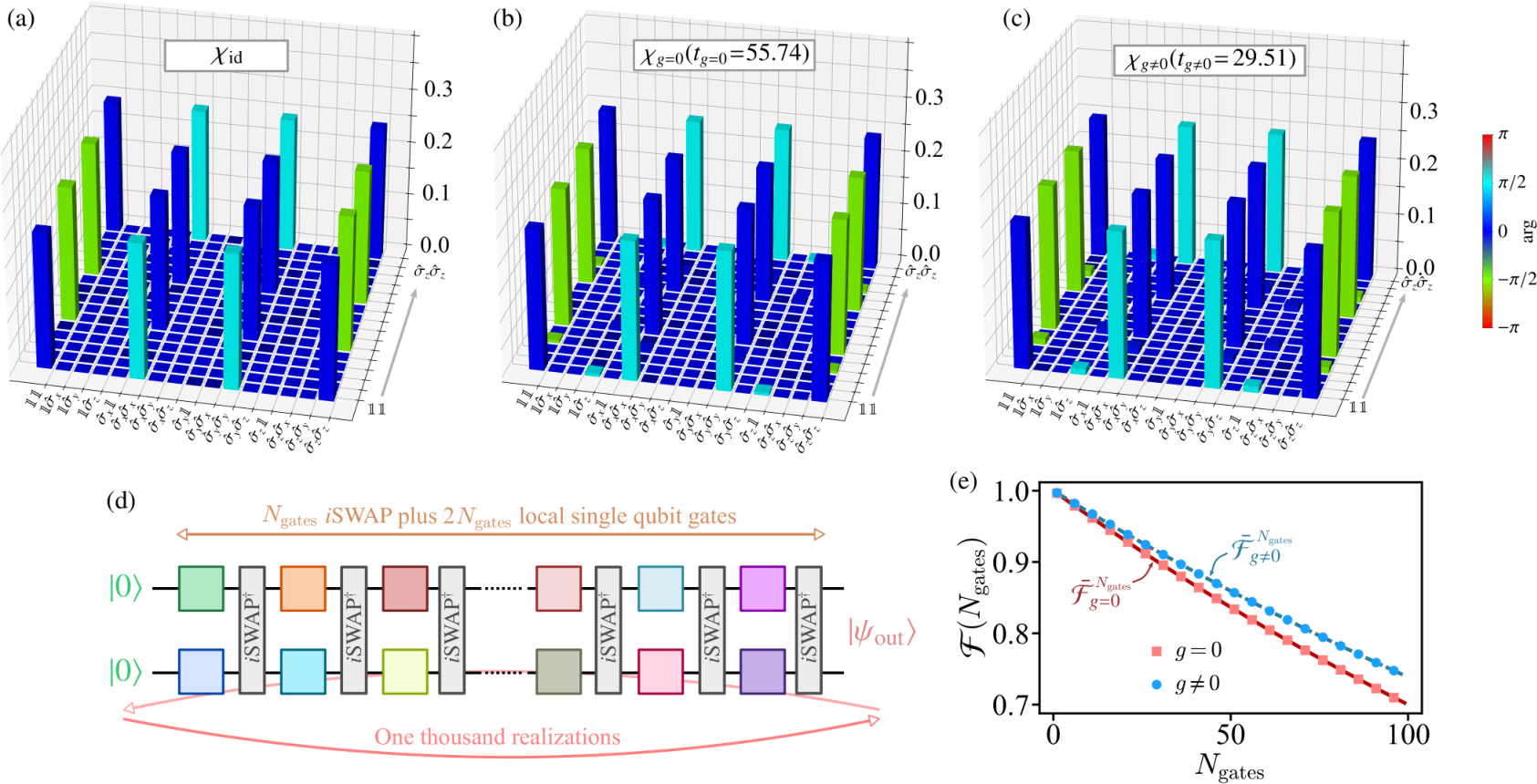
The average fidelity of each dynamics ($g=0$ and $g\neq 0$) with respect to the ideal one is addressed through the randomized benchmarking, as sketched in Fig. 4d. It is desired here to measure the average fidelity $i$SWAP gate, so the circuit is comprised for $N_{\mathrm{gates}}$ $i$SWAP gates interspersed with local single qubit gates. The random property of the circuit is encoded in the generic local qubit gates written as $G_{\mathrm{local}}=G_{1}(\theta_{1},\phi_{1},\lambda_{1})\otimes G_{2}(\theta_{2},\phi_{2},\lambda_{2})$ with

acting on the $k$-th qubit, and the triplet $\theta_{k}$, $\phi_{k}$ and $\lambda_{k}$ is randomly chosen in the interval $[0,2\pi]$, $[0,\pi]$ and $[0,\pi]$, respectively, for each step of the circuit in Fig. 4d.

By measuring fidelity of a single realization from the Bures metric for pure states Nielsen and Chuang 2011, $\mathcal{F}_{g=0}(\psi,\psi^{\prime})=|\bra*{\psi}\ket*{\psi^{\prime}}|^{2}$, we then average the circuit over one thousand of realizations. We define the fidelities $\mathcal{F}_{g=0}=\mathcal{F}(\psi_{\mathrm{ideal}},\psi_{g=0})$ and $\mathcal{F}_{g\neq 0}=\mathcal{F}(\psi_{\mathrm{ideal}},\psi_{g\neq 0})$ for each dynamics, in which $\ket{\psi_{\mathrm{ideal}}}$ is the ideal expected computation outcome and $\ket*{\psi_{g = 0}}$ ($\ket*{\psi_{g \neq 0}}$) is the simulation output with no parasitic interaction $g=0$ (with parasitic interaction $g\neq 0$). Fig. 4e shows the result for a circuit with up to $100$ $i$SWAP gates (plus $100$ pairs of local qubit gates $G_{\mathrm{local}}$). Therefore, by fitting the set of data to determine the average success fidelity $\bar{\mathcal{F}}$ of a $i$SWAP gate after $N_{\mathrm{gates}}$ of the circuit, in Fig. 4d, according to the fit $\mathcal{F}(N_{\mathrm{gates}})=\bar{\mathcal{F}}^{N_{\mathrm{gates}}}$, one gets the respective fidelities $\bar{\mathcal{F}}_{g=0}=99.64(4)$ and $\bar{\mathcal{F}}_{g\neq 0}=99.69(7)$. These values are achieved after many realizations, which means that for a single realization such values will be different. However, the main result after this analysis is that the effects parasitic interaction in such a system can be efficiently suppressed if we know its strength.

References

- Song et al. (2017) C. Song, et al., “10-Qubit Entanglement and Parallel Logic Operations with a Superconducting Circuit”, Phys. Rev. Lett. 119, 180511 (2017).
- Gong et al. (2019) M. Gong, et al., “Genuine 12-Qubit Entanglement on a Superconducting Quantum Processor”, Phys. Rev. Lett. 122, 110501 (2019).
- Arute et al. (2019) F. Arute, et al., “Quantum supremacy using a programmable superconducting processor”, Nature 574, 505 (2019).
- Wu et al. (2021) Y. Wu, et al., “Strong Quantum Computational Advantage Using a Superconducting Quantum Processor”, Phys. Rev. Lett. 127, 180501 (2021).
- Gong et al. (2021) M. Gong, et al., “Experimental characterization of the quantum many-body localization transition”, Phys. Rev. Research 3, 033043 (2021).
- Wendin (2017) G. Wendin, “Quantum information processing with superconducting circuits: a review”, Reports on Progress in Physics 80, 106001 (2017).
- Siddiqi (2021) I. Siddiqi, “Engineering high-coherence superconducting qubits”, Nature Reviews Materials 6, 875 (2021).
- Burnett et al. (2019) J. J. Burnett, et al., “Decoherence benchmarking of superconducting qubits”, npj Quantum Information 5, 1 (2019).
- Zhao et al. (2022a) P. Zhao, et al., “Quantum Crosstalk Analysis for Simultaneous Gate Operations on Superconducting Qubits”, PRX Quantum 3, 020301 (2022a).
- Willsch et al. (2017) D. Willsch, et al., “Gate-error analysis in simulations of quantum computers with transmon qubits”, Phys. Rev. A 96, 062302 (2017).
- Krinner et al. (2020) S. Krinner, et al., “Benchmarking Coherent Errors in Controlled-Phase Gates due to Spectator Qubits”, Phys. Rev. Applied 14, 024042 (2020).
- Han et al. (2020) X. Y. Han, et al., “Error analysis in suppression of unwanted qubit interactions for a parametric gate in a tunable superconducting circuit”, Phys. Rev. A 102, 022619 (2020).
- Dai et al. (2022) X. Dai, et al., “Optimizing for periodicity: a model-independent approach to flux crosstalk calibration for superconducting circuits”, arXiv e-prints , arXiv:2211.01497 (2022), arXiv:2211.01497 [quant-ph] .
- Córcoles et al. (2015) A. D. Córcoles, et al., “Demonstration of a quantum error detection code using a square lattice of four superconducting qubits”, Nature communications 6, 1 (2015).
- Tripathi et al. (2022) V. Tripathi, et al., “Suppression of Crosstalk in Superconducting Qubits Using Dynamical Decoupling”, Phys. Rev. Applied 18, 024068 (2022).
- Chen et al. (2021) Z. Chen, et al., “Exponential suppression of bit or phase errors with cyclic error correction”, Nature 595, 383 (2021).
- Zhao et al. (2022b) Y. Zhao, et al., “Realization of an Error-Correcting Surface Code with Superconducting Qubits”, Phys. Rev. Lett. 129, 030501 (2022b).
- Mates et al. (2019) J. Mates, et al., “Crosstalk in microwave SQUID multiplexers”, Applied Physics Letters 115, 202601 (2019).
- Mundada et al. (2019) P. Mundada, G. Zhang, T. Hazard, and A. Houck, “Suppression of Qubit Crosstalk in a Tunable Coupling Superconducting Circuit”, Phys. Rev. Applied 12, 054023 (2019).
- Dai et al. (2021) X. Dai, et al., “Calibration of Flux Crosstalk in Large-Scale Flux-Tunable Superconducting Quantum Circuits”, PRX Quantum 2, 040313 (2021).
- Ni et al. (2022) Z. Ni, et al., “Scalable Method for Eliminating Residual Interaction between Superconducting Qubits”, Phys. Rev. Lett. 129, 040502 (2022).
- Cai et al. (2021a) T.-Q. Cai, et al., “Impact of Spectators on a Two-Qubit Gate in a Tunable Coupling Superconducting Circuit”, Phys. Rev. Lett. 127, 060505 (2021a).
- Nuerbolati et al. (2022) W. Nuerbolati, et al., “Canceling microwave crosstalk with fixed-frequency qubits”, Applied Physics Letters 120, 174001 (2022).
- Sheldon et al. (2016) S. Sheldon, E. Magesan, J. M. Chow, and J. M. Gambetta, “Procedure for systematically tuning up cross-talk in the cross-resonance gate”, Phys. Rev. A 93, 060302 (2016).
- Blais et al. (2004) A. Blais, et al., “Cavity quantum electrodynamics for superconducting electrical circuits: An architecture for quantum computation”, Phys. Rev. A 69, 062320 (2004).
- Blais et al. (2007) A. Blais, et al., “Quantum-information processing with circuit quantum electrodynamics”, Phys. Rev. A 75, 032329 (2007).
- Wallraff et al. (2004) A. Wallraff, et al., “Strong coupling of a single photon to a superconducting qubit using circuit quantum electrodynamics”, Nature 431, 162 (2004).
- Majer et al. (2007) J. Majer, et al., “Coupling superconducting qubits via a cavity bus”, Nature 449, 443 (2007).
- Chow et al. (2011) J. M. Chow, et al., “Simple All-Microwave Entangling Gate for Fixed-Frequency Superconducting Qubits”, Phys. Rev. Lett. 107, 080502 (2011).
- DiCarlo et al. (2009) L. DiCarlo, et al., “Demonstration of two-qubit algorithms with a superconducting quantum processor”, Nature 460, 240 (2009).
- Johnson et al. (2010) B. Johnson, et al., “Quantum non-demolition detection of single microwave photons in a circuit”, Nature Physics 6, 663 (2010).
- Leek et al. (2010) P. J. Leek, et al., “Cavity Quantum Electrodynamics with Separate Photon Storage and Qubit Readout Modes”, Phys. Rev. Lett. 104, 100504 (2010).
- McKay et al. (2019) D. C. McKay, et al., “Three-Qubit Randomized Benchmarking”, Phys. Rev. Lett. 122, 200502 (2019).
- Cai et al. (2021b) T.-Q. Cai, et al., “All-microwave nonadiabatic multiqubit geometric phase gate for superconducting qubits”, Phys. Rev. Research 3, 043071 (2021b).
- Fink et al. (2009) J. M. Fink, et al., “Dressed Collective Qubit States and the Tavis-Cummings Model in Circuit QED”, Phys. Rev. Lett. 103, 083601 (2009).
- Wang et al. (2020) Z. Wang, et al., “Controllable Switching between Superradiant and Subradiant States in a 10-qubit Superconducting Circuit”, Phys. Rev. Lett. 124, 013601 (2020).
- Blais et al. (2021) A. Blais, A. L. Grimsmo, S. M. Girvin, and A. Wallraff, “Circuit quantum electrodynamics”, Rev. Mod. Phys. 93, 025005 (2021).
- Berke et al. (2022) C. Berke, et al., “Transmon platform for quantum computing challenged by chaotic fluctuations”, Nature communications 13, 1 (2022).
- Xu et al. (2020) Y. Xu, et al., “High-Fidelity, High-Scalability Two-Qubit Gate Scheme for Superconducting Qubits”, Phys. Rev. Lett. 125, 240503 (2020).
- Chu et al. (2022) J. Chu, et al., “Scalable algorithm simplification using quantum AND logic”, Nature Physics (2022), 10.1038/s41567-022-01813-7.
- Luo et al. (2022) K. Luo, et al., “Experimental Realization of Two Qutrits Gate with Tunable Coupling in Superconducting Circuits”, arXiv e-prints , arXiv:2206.11199 (2022), arXiv:2206.11199 [quant-ph] .
- Hu et al. (2022) C.-K. Hu, et al., “Conditional coherent control with superconducting artificial atoms”, arXiv e-prints , arXiv:2203.09791 (2022), arXiv:2203.09791 [quant-ph] .
- Mitchell et al. (2021) B. K. Mitchell, et al., “Hardware-Efficient Microwave-Activated Tunable Coupling between Superconducting Qubits”, Phys. Rev. Lett. 127, 200502 (2021).
- Klink (1997) W. Klink, “Quantum Mechanics in Nonintertial Reference Frames”, Annals of Physics 260, 27 (1997).
- Serov (2017) V. Serov, “The Riemann–Lebesgue Lemma”, in Fourier Series, Fourier Transform and Their Applications to Mathematical Physics (Springer International Publishing, Cham, 2017) pp. 33–35.
- Bravyi et al. (2011) S. Bravyi, D. P. DiVincenzo, and D. Loss, “Schrieffer–Wolff transformation for quantum many-body systems”, Annals of Physics 326, 2793 (2011).
- Yan et al. (2018) F. Yan, et al., “Tunable Coupling Scheme for Implementing High-Fidelity Two-Qubit Gates”, Phys. Rev. Applied 10, 054062 (2018).
- Li et al. (2020) X. Li, et al., “Tunable Coupler for Realizing a Controlled-Phase Gate with Dynamically Decoupled Regime in a Superconducting Circuit”, Phys. Rev. Applied 14, 024070 (2020).
- Feng and Wang (2020) W. Feng and D.-w. Wang, “Quantum Fredkin gate based on synthetic three-body interactions in superconducting circuits”, Phys. Rev. A 101, 062312 (2020).
- Johansson et al. (2012) J. Johansson, P. Nation, and F. Nori, “QuTiP: An open-source Python framework for the dynamics of open quantum systems”, Computer Physics Communications 183, 1760 (2012).
- Johansson et al. (2013) J. Johansson, P. Nation, and F. Nori, “QuTiP 2: A Python framework for the dynamics of open quantum systems”, Computer Physics Communications 184, 1234 (2013).
- Nielsen and Chuang (2011) M. A. Nielsen and I. L. Chuang, Quantum Computation and Quantum Information: 10th Anniversary Edition, 10th ed. (Cambridge University Press, New York, NY, USA, 2011).
- Yurtalan et al. (2020) M. A. Yurtalan, et al., “Implementation of a Walsh-Hadamard Gate in a Superconducting Qutrit”, Phys. Rev. Lett. 125, 180504 (2020).
- Kononenko et al. (2021) M. Kononenko, et al., “Characterization of control in a superconducting qutrit using randomized benchmarking”, Phys. Rev. Research 3, L042007 (2021).
- Goss et al. (2022) N. Goss, et al., “High-Fidelity Qutrit Entangling Gates for Superconducting Circuits”, Nature Communications 13, 1 (2022).
- Xue et al. (2017) Z.-Y. Xue, et al., “Nonadiabatic Holonomic Quantum Computation with Dressed-State Qubits”, Phys. Rev. Applied 7, 054022 (2017).
- Li et al. (2021) S. Li, et al., “Superrobust Geometric Control of a Superconducting Circuit”, Phys. Rev. Applied 16, 064003 (2021).
- Ma et al. (2022) Z. Ma, et al., “Experimental Implementation of Noncyclic and Nonadiabatic Geometric Quantum Gates in a Superconducting Circuit”, arXiv e-prints , arXiv:2210.03326 (2022), arXiv:2210.03326 [quant-ph] .
- Hu et al. (2022) C.-K. Hu, et al., “Optimal charging of a superconducting quantum battery”, Quantum Science and Technology 7, 045018 (2022).