跳到论文正文
W Papers独立论文阅读器 arXiv:2211.04171 论文正文 计算阅读时间 · 0%
引用这篇论文根据当前论文元数据生成,正式投稿前建议核对。


License: arXiv.org perpetual non-exclusive license
arXiv:2211.04171v3 [math.OC] 02 Jan 2023

The Hypervolume Indicator Hessian Matrix: Analytical Expression, Computational Time Complexity, and Sparsity

André H. Deutz Affiliation: Leiden Institute of Advanced Computer Science Affiliation: Leiden University Affiliation: 2333CA Leiden Affiliation: The Netherlands    Michael T.M. Emmerich Affiliation: Leiden Institute of Advanced Computer Science Affiliation: Leiden University Affiliation: 2333CA Leiden Affiliation: The Netherlands    Hao Wang Affiliation: Leiden Institute of Advanced Computer Science Affiliation: and applied Quantum algorithms (aQa) Affiliation: Leiden University Affiliation: 2333CA Leiden Affiliation: The Netherlands
Abstract

The problem of approximating the Pareto front of a multiobjective optimization problem can be reformulated as the problem of finding a set that maximizes the hypervolume indicator. This paper establishes the analytical expression of the Hessian matrix of the mapping from a (fixed size) collection of nn points in the dd-dimensional decision space (or mm dimensional objective space) to the scalar hypervolume indicator value. To define the Hessian matrix, the input set is vectorized, and the matrix is derived by analytical differentiation of the mapping from a vectorized set to the hypervolume indicator. The Hessian matrix plays a crucial role in second-order methods, such as the Newton-Raphson optimization method, and it can be used for the verification of local optimal sets. So far, the full analytical expression was only established and analyzed for the relatively simple bi-objective case. This paper will derive the full expression for arbitrary dimensions (m≥2m\geq 2 objective functions). For the practically important three-dimensional case, we also provide an asymptotically efficient algorithm with time complexity in O⁡(n​log⁡n)O(n\log n) for the exact computation of the Hessian Matrix’ non-zero entries. We establish a sharp bound of 12​m−612m-6 for the number of non-zero entries. Also, for the general mm-dimensional case, a compact recursive analytical expression is established, and its algorithmic implementation is discussed. Also, for the general case, some sparsity results can be established; these results are implied by the recursive expression. To validate and illustrate the analytically derived algorithms and results, we provide a few numerical examples using Python and Mathematica implementations. Open-source implementations of the algorithms and testing data are made available as a supplement to this paper.

1 Introduction

Symbol Domain or Signature Description
mm ℕ\mathbb{N} number of objective functions
dd ℕ\mathbb{N} number of decision variables
nn ℕ\mathbb{N} number of points in the approximation set
𝐟=(f1,…,fm)\mathbf{f}=(f_{1},\dots,f_{m}) ℝd→ℝm\mathbb{R}^{d}\rightarrow\mathbb{R}^{m} vector-valued objective function
𝐗=(𝐱(1)⊤,…,𝐱(n)⊤)⊤\mathbf{X}=({\mathbf{x}^{(1)}}^{\top},\ldots,{\mathbf{x}^{(n)}}^{\top})^{\top} ℝn​d\mathbb{R}^{nd} concatenation of nn points in the decision space
𝐘=(𝐲(1)⊤,…,𝐲(n)⊤)⊤\mathbf{Y}=({\mathbf{y}^{(1)}}^{\top},\ldots,{\mathbf{y}^{(n)}}^{\top})^{\top} ℝn​m\mathbb{R}^{nm} concatenation of nn points in the objective space
λm\lambda_{m} ℬ⁡(ℝn)→ℝ≥0\mathcal{B}(\mathbb{R}^{n})\rightarrow\mathbb{R}_{\geq 0} mm-dimensional Lebesgue measure
HV\operatorname{HV} ℬ⁡(ℝn)→ℝ≥0\mathcal{B}(\mathbb{R}^{n})\rightarrow\mathbb{R}_{\geq 0} HVI for subsets of the objective space
ℋ\mathcal{H} ℝn​m→ℝ≥0\mathbb{R}^{nm}\rightarrow\mathbb{R}_{\geq 0} HVI supported on the product of nn objective spaces
ℋ𝐅\mathcal{H}_{\mathbf{F}} ℝn​d→ℝ≥0\mathbb{R}^{nd}\rightarrow\mathbb{R}_{\geq 0} HVI supported on the product of nn decision spaces
Table 1: Basic notation used throughout the paper. HVI stands for “Hypervolume Indicator”. ℬ⁡(ℝn)\mathcal{B}(\mathbb{R}^{n}) denotes the Borel sets on ℝn\mathbb{R}^{n}.

In this paper, we delve into continuous mm-dimensional multi-objective optimization problems (MOPs), where multiple objective functions, e.g., 𝐟=(f1,…,fm):𝒳⊆ℝd→ℝm\mathbf{f}=(f_{1},\ldots,f_{m}):\mathcal{X}\subseteq\mathbb{R}^{d}\rightarrow\mathbb{R}^{m} are subject to minimization. Also, we assume 𝐟\mathbf{f} is at least twice continuously differentiable. When solving such problems, it is a common strategy to approximate the Pareto front for mm-objective functions mapping from a continuous decision space ℝd\mathbb{R}^{d} to the ℝ\mathbb{R} (or as a vector-valued function from ℝd\mathbb{R}^{d} to ℝm\mathbb{R}^{m}. MOPs can be accomplished by means of a finite set of points that distributes across the at most m−1m-1-dimensional manifold of the Pareto front. The hypervolume indicator of a set of points is the mm dimensional Lebesgue measure of the space that is jointly dominated by a set of objective function vectors in ℝm\mathbb{R}^{m} and bound from above by a reference point 𝐫∈ℝm\mathbf{r}\in\mathbb{R}^{m}. More precisely, for minimization problems, the hypervolume indicator (HV) [ZT98, ZTL+03] is defined as the Lebesgue measure of the compact set dominated by a Pareto approximation set Y⊂ℝmY\subset\mathbb{R}^{m} and cut from above by a reference point 𝐫\mathbf{r}:

HV⁡(Y;𝐫)=λm​({𝐩:∃𝐲∈Y⁡(𝐲≺𝐩∧𝐩≺𝐫)}),\operatorname{HV}(Y;\mathbf{r})=\lambda_{m}\left(\left\{\mathbf{p}\colon\exists\mathbf{y}\in Y(\mathbf{y}\prec\mathbf{p}\wedge\mathbf{p}\prec\mathbf{r})\right\}\right),

where λm\lambda_{m} denotes the Lebesgue measure on measurable space (ℝm,B⁡(ℝm))(\mathbb{R}^{m},B(\mathbb{R}^{m})) with B⁡(ℝm)B(\mathbb{R}^{m}) being the Borel sets of ℝm\mathbb{R}^{m}. We will omit the reference point for simplicity henceforth. HV is Pareto compliant, i.e., for all Y≺Y′Y\prec Y^{\prime}, HV⁡(Y)>HV⁡(Y′)\operatorname{HV}(Y)>\operatorname{HV}(Y^{\prime}), and is extensively used to assess the quality of approximation sets to the Pareto front, e.g., in SMS-EMOA [BNE07] and multiobjective Bayesian optimization [EYD+16]. Being a set function, it is cumbersome to define the derivative of HV11 1 The derivative of a set function is not defined for an arbitrary family of sets. For some special cases, it can be defined directly, e.g., on Jordan-measurable sets [DD02].. Therefore, we follow the generic set-based approach for MOPs [ED12], which considers a finite set of objective points (of size nn) as a single point in ℝn​m\mathbb{R}^{nm}, obtained via the following concatenation map (and its inverse):

concat\displaystyle\operatorname{concat} :(ℝm)n→ℝn​m,Y↦(y1(1),…,ym(1),…,y1(n),…,ym(n))⊤,\displaystyle\colon(\mathbb{R}^{m})^{n}\rightarrow\mathbb{R}^{nm},\quad Y\mapsto\left(y_{1}^{(1)},\ldots,y_{m}^{(1)},\ldots,y_{1}^{(n)},\ldots,y_{m}^{(n)}\right)^{\top},
concat−1\displaystyle\operatorname{concat}^{-1} :ℝn​m→(ℝm)n,𝐘↦{(Y1,…,Ym)⊤,(Ym+1,…,Y2​m)⊤,…,(Y(n−1)​m+1,…,Yn​m)⊤}.\displaystyle\colon\mathbb{R}^{nm}\rightarrow(\mathbb{R}^{m})^{n},\quad\mathbf{Y}\mapsto\left\{(Y_{1},\ldots,Y_{m})^{\top},(Y_{m+1},\ldots,Y_{2m})^{\top},\ldots,(Y_{(n-1)m+1},\ldots,Y_{nm})^{\top}\right\}.

The concatenation map gives rise to a hypervolume function that takes vectors in ℝn​m\mathbb{R}^{nm} as input:

ℋ:ℝn​m→ℝ≥0,𝐘↦[HV∘concat−1]​(𝐘),\mathcal{H}\colon\mathbb{R}^{nm}\rightarrow\mathbb{R}_{\geq 0},\quad\mathbf{Y}\mapsto\left[\operatorname{HV}\circ\operatorname{concat}^{-1}\right](\mathbf{Y}), (1)

Similarly, we also consider a finite set of decision points (of size nn) as a single point in ℝn​d\mathbb{R}^{nd}, i.e., 𝐗=[𝐱(1)⊤,𝐱(2)⊤,…,𝐱(n)⊤]⊤∈ℝn​d\mathbf{X}=[{\mathbf{x}^{(1)}}^{\top},{\mathbf{x}^{(2)}}^{\top},\ldots,{\mathbf{x}^{(n)}}^{\top}]^{\top}\in\mathbb{R}^{nd}. In this sense, the objective function 𝐟\mathbf{f} is also extended to:

𝐅:𝒳n→ℝn​m,𝐗↦[𝐟⁡(X1,…,Xd),𝐟⁡(Xd+1,…,X2​d),…,𝐟⁡(X(n−1)​d+1,…,Xn​d)]⊤.\mathbf{F}\colon\mathcal{X}^{n}\rightarrow\mathbb{R}^{nm},\mathbf{X}\mapsto[\mathbf{f}(X_{1},\ldots,X_{d}),\mathbf{f}(X_{d+1},\ldots,X_{2d}),\ldots,\mathbf{f}(X_{(n-1)d+1},\ldots,X_{nd})]^{\top}.

Given 𝐅\mathbf{F}, we have the relation 𝐘=𝐅⁡(𝐗)\mathbf{Y}=\mathbf{F}(\mathbf{X}). Now, we can express hypervolume indicator as a function supported on ℝn​d\mathbb{R}^{nd}:

ℋ𝐅:ℝn​d→ℝ≥0,𝐗↦[HV∘concat−1∘𝐅]​(𝐗).\mathcal{H}_{\mathbf{F}}\colon\mathbb{R}^{nd}\rightarrow\mathbb{R}_{\geq 0},\quad\mathbf{X}\mapsto\left[\operatorname{HV}\circ\operatorname{concat}^{-1}\circ\mathbf{F}\right](\mathbf{X}). (2)

Notably, assuming 𝐟\mathbf{f} is twice differentiable, the above hypervolume functions ℋ\mathcal{H} and ℋ𝐅\mathcal{H}_{\mathbf{F}} are twice differentiable almost everywhere in their domains, respectively.

It is straightforward to express the gradient of ℋ𝐅\mathcal{H}_{\mathbf{F}} w.r.t. 𝐗\mathbf{X} using the chain rule as reported in our previous works [ED12, WDBE17]: ∇ℋ𝐅​(𝐗)=(∂ℋ/∂𝐘)​(∂𝐅⁡(𝐗)/∂𝐗)\nabla\mathcal{H}_{\mathbf{F}}(\mathbf{X})=(\partial\mathcal{H}/\partial\mathbf{Y})(\partial\mathbf{F}(\mathbf{X})/\partial\mathbf{X}), in which we also discussed the time complexity of computing the hypervolume gradient.

In this work, we investigate the Hypervolume Indicator Hessian Matrix for more than two objectives and propose an algorithm to compute it efficiently. The work is structured as follows: In Section 2, we briefly review the general construction of the Hypervolume Gradient and Hypervolume Hessian ℋ𝐅\mathcal{H}_{\mathbf{F}} via the chain-rule as it has been outlined previously in [ED12] and, respectively, in [SSW+20]. Section 3 provides a discussion of the 3-D Hypervolume indicator Hessian matrix HV\operatorname{HV}, including a O⁡(n​log⁡n)O(n\log n) dimension sweep algorithm for its asymptotically optimal computation and an analysis of its sparsity, i.e., the number of its non-zero components. Furthermore, it is argued that in the 3-D case, the Hypervolume Hessian Matrix is sparse and has at most O⁡(n)O(n) non-zero components. In Section 4, we discuss the analytical formulations of the hypervolume Hessian for the general case of m>1m>1 objective functions. The result reduces the computation of the Hessian of mm objective functions to the repeated computation of the hypervolume indicator gradient for collections of vectors in ℝm−1\mathbb{R}^{m-1}. A Python implementation is provided for the general cases. In Section 5, we provide numerical examples. In Section 6, we finish the paper with a discussion of some basic properties of the hypervolume Hessian matrix, such as its continuity, one-sidedness, and rank, and point out interesting open questions for its further analysis.

2 General Construction of Hypervolume Hessian and Gradient via the Chain Rule

Taking the ℝn​d\mathbb{R}^{nd}-vector 𝐗\mathbf{X} and ℝn​m\mathbb{R}^{nm}-vector 𝐘=𝐅⁡(𝐗)\mathbf{Y}=\mathbf{F}(\mathbf{X}), we express the Hessian matrix of the hypervolume indicator as follows:

∇2ℋ𝐅\displaystyle\nabla^{2}\mathcal{H}_{\mathbf{F}} =∂∂𝐗​(∂ℋ∂𝐘​∂𝐘∂𝐗)=[∂∂𝐗​(∂ℋ∂𝐘)]⊤​∂𝐅⁡(𝐗)∂𝐗+∂ℋ∂𝐘​∂2𝐅⁡(𝐗)∂𝐗​∂𝐗⊤\displaystyle=\frac{\partial}{\partial\mathbf{X}}\left(\frac{\partial\mathcal{H}}{\partial\mathbf{Y}}\frac{\partial\mathbf{Y}}{\partial\mathbf{X}}\right)=\left[\frac{\partial}{\partial\mathbf{X}}\left(\frac{\partial\mathcal{H}}{\partial\mathbf{Y}}\right)\right]^{\top}\frac{\partial\mathbf{F}(\mathbf{X})}{\partial\mathbf{X}}+\frac{\partial\mathcal{H}}{\partial\mathbf{Y}}\frac{\partial^{2}\mathbf{F}(\mathbf{X})}{\partial\mathbf{X}\partial\mathbf{X}^{\top}}
=∇𝐅(𝐗)⊤∂2ℋ∂𝐘​∂𝐘⊤∇𝐅(𝐗)+∂ℋ∂𝐘∂2𝐅⁡(𝐗)∂𝐗​∂𝐗⊤.\displaystyle=\nabla{\mathbf{F}(\mathbf{X})}^{\top}\frac{\partial^{2}\mathcal{H}}{\partial\mathbf{Y}\partial\mathbf{Y}^{\top}}\nabla{\mathbf{F}(\mathbf{X})}+\frac{\partial\mathcal{H}}{\partial\mathbf{Y}}\frac{\partial^{2}\mathbf{F}(\mathbf{X})}{\partial\mathbf{X}\partial\mathbf{X}^{\top}}. (3)

The Hessian of vector-valued objective function 𝐅\mathbf{F}, i.e., ∂2𝐅/∂𝐗​∂𝐗⊤:ℝn​d→Hom⁡(ℝn​d,Hom⁡(ℝn​d,ℝn​m))\partial^{2}\mathbf{F}/\partial\mathbf{X}\partial\mathbf{X}^{\top}\colon\mathbb{R}^{nd}\rightarrow\Hom(\mathbb{R}^{nd},\Hom(\mathbb{R}^{nd},\mathbb{R}^{nm})), is a tensor of (1,2)(1,2) type. Let Ti,jk=∂2Fk/∂Xi∂Xj,i,j∈[1..nd],k∈[1..nm]T^{k}_{i,j}=\partial^{2}F_{k}/\partial\mathrm{X}_{i}\partial\mathrm{X}_{j},i,j\in[1..nd],k\in[1..nm], we specify the entries of TT as follows:

Ti,jk={∂2fβ​(𝐱(α))/∂xi′(α)​∂xj′(α),if (α−1)d+1≤i,j≤αd,0,otherwise.\displaystyle T^{k}_{i,j}=\begin{cases}\partial^{2}f_{\beta}(\mathbf{x}^{(\alpha)})/\partial x^{(\alpha)}_{i^{\prime}}\partial x^{(\alpha)}_{j^{\prime}},&\text{if }(\alpha-1)d+1\leq i,j\leq\alpha d,\\ 0,&\text{otherwise.}\end{cases}
α=⌈k/m⌉,β=k−(α−1)​m,i′=i−(α−1)​d,j′=j−(α−1)​d.\displaystyle\alpha=\lceil k/m\rceil,\beta=k-(\alpha-1)m,i^{\prime}=i-(\alpha-1)d,j^{\prime}=j-(\alpha-1)d.

Since the above map from kk to (α,β)(\alpha,\beta) is bijective (its inverse is k=α​βk=\alpha\beta), we will equivalently use α​β\alpha\beta for the contravariant index kk. It is obvious that tensor TT is sparse, where for each kk, only d2d^{2} entries are nonzero, giving up to n​m​d2nmd^{2} nonzero entries in total. Using the Einstein summation convention, we can expand the second term in Eq. (3) as:

(∂ℋ∂𝐘​∂2𝐅⁡(𝐗)∂𝐗​∂𝐗⊤)i,j=(∂ℋ∂𝐘)k​Ti,jk=∂ℋ∂fβ​(𝐱(α))​Ti,jα​β,\left(\frac{\partial\mathcal{H}}{\partial\mathbf{Y}}\frac{\partial^{2}\mathbf{F}(\mathbf{X})}{\partial\mathbf{X}\partial\mathbf{X}^{\top}}\right)_{i,j}=\left(\frac{\partial\mathcal{H}}{\partial\mathbf{Y}}\right)_{k}T^{k}_{i,j}=\frac{\partial\mathcal{H}}{\partial f_{\beta}(\mathbf{x}^{(\alpha)})}T^{\alpha\beta}_{i,j}, (4)

where (⋅)i,j(\cdot)_{i,j} denotes the (i,j)(i,j)-entry of a tensor. We have discussed the analytical expression of the term ∂ℋ/∂𝐘\partial\mathcal{H}/\partial\mathbf{Y} in our previous works [ED12, WDBE17]. Notably, the above expression leads to a block-diagonal matrix containing nn matrices of shape d×dd\times d on its diagonal. Therefore, we observe a high sparsity of the second term in Eq. (3). As for the first term, ∂2ℋ/∂𝐘​∂𝐘⊤\partial^{2}\mathcal{H}/\partial\mathbf{Y}\partial\mathbf{Y}^{\top} denotes the Hessian of the hypervolume indicator w.r.t. objective vectors, whose computation and sparsity will be discussed in the following sections.
In our previous work [SSW+20], we have derived the analytical expression of ∇2ℋ𝐅\nabla^{2}\mathcal{H}_{\mathbf{F}} for bi-objective cases and analyzed the structure and properties of the hypervolume Hessian matrix. Also, we implemented a standalone Hypervolume Newton (HVN) algorithm for unconstrained MOPs. Moreover, we have shown that the Hessian ∇2ℋ𝐅\nabla^{2}\mathcal{H}_{\mathbf{F}} is a tri-diagonal block matrix in bi-objective cases and provided the non-singularity condition thereof, which states the Hessian is only singular on a null subset of ℝn​d\mathbb{R}^{nd} [SSW+20], thereby ascertaining the safety of utilizing hypervolume Hessian matrix, e.g., in the hypervolume Newton method [WED+22] for equality constraints.

3 Hypervolume Indicator Hessian Matrix in 3-D

As with many problems related to Pareto dominance, the 2-D and 3-D cases have a special structure that can be exploited for formulating asymptotically efficient dimension sweep algorithms [KLP75, PSSL22]. Next, the dimension sweep technique will be applied to yield an asymptotically efficient algorithm for the problem of computing the Hessian Matrix of the 3-D Hypervolume Indicator HV\operatorname{HV}. The basic idea is sketched in Fig. 3 and consists of computing first the facets of the polyhedron that is measured by the hypervolume indicator by lowering a sweeping plane along each one of the axes. The gradient components are given by the areas of the facets (e.g., the yellow shaded area in Fig. 3, and the length of the line segments of the ortho-convex polygon that surrounds this facet determines the components of the Hessian matrix of HV\operatorname{HV}. This can be easily verified by studying geometrically the effect of small perturbations of the coordinates of points in 𝐘\mathbf{Y} along the coordinate axis on the value of the hypervolume indicator (gradient components) HV\operatorname{HV}.

[Uncaptioned image]\captionof

figureVisualization of some first and second-order derivatives of a 3-D Hypervolume approximation set (𝐲(1),𝐲(2),𝐲(3))(\mathbf{y}^{(1)},\mathbf{y}^{(2)},\mathbf{y}^{(3)}) with i​1i1, i​2i2, i​3i3 chosen such that y3(i​1)y^{(i1)}_{3} >> y3(i​2)y^{(i2)}_{3} >> y3(i​3)y^{(i3)}_{3}.

012345678012345678𝐲(0)\mathbf{y}^{(0)}𝐲(i​5)=𝐝t(0)\mathbf{y}^{(i5)}=\mathbf{d}_{t}^{(0)}𝐲(i​7)\mathbf{y}^{(i7)}𝐲(i​4)=𝐝t(Nt+1)\mathbf{y}^{(i4)}=\mathbf{d}_{t}^{(N_{t}+1)}𝐲(i​3)=𝐝t(1)\mathbf{y}^{(i3)}=\mathbf{d}_{t}^{(1)}𝐲(i​2)=𝐝t(2)\mathbf{y}^{(i2)}=\mathbf{d}_{t}^{(2)}𝐲(i​1)\mathbf{y}^{(i1)}𝐭(2)\mathbf{t}^{(2)}𝐭(1)\mathbf{t}^{(1)}𝐫\mathbf{r}𝐲(n+1)\mathbf{y}^{(n+1)}\captionof

figureSnapshot of the components of the polygon (yellow shaded), in which the length of each edge constitutes the non-zero components of the Hessian matrix of HV\operatorname{HV} in a single iteration (lowering of sweeping plane) tt of Alg. 1.

Without loss of generality, we first compute the derivatives with respect to y3y_{3}. By permuting the roles of y1y_{1}, y2y_{2}, and y3y_{3}, we can get all derivatives. In the context of the dimension sweep algorithm, we assume that points in Fig. 3 are sorted by the 3rd coordinate y3y_{3}, that is, YY is represented in such a way that y3(i​3)<y3(i​2)<y3(i​1)y^{(i3)}_{3}<y^{(i2)}_{3}<y^{(i1)}_{3}. We assume that the points in 𝐘\mathbf{Y} are in general position (otherwise, one-sided derivatives can occur, which will be discussed later).

Alg. 1 computes all positive entries of the Hessian matrix of HV\operatorname{HV} at a point Y\mathrm{Y}. The algorithm proceeds in three sweeps. The sweep coordinate has index hh (like height), and the other two coordinates are termed ll and ww (like length and width). The first sweep sets h=3h=3, the second sweep h=2h=2, and the third sweep h=1h=1. The values of ll and ww are set to the remaining two coordinates. The roles of ll and ww are interchangeable, but here we set them to l=1l=1, w=2w=2 in the first sweep, to l=1,w=3l=1,w=3 in the second sweep, and to l=3,w=2l=3,w=2 in the third sweep. Next, we describe a single sweep in detail. Without loss of generality, let us choose the sweep along the 3-rd coordinate, e.g., l=1,w=2,h=3l=1,w=2,h=3: First, we introduce sentinels 𝐲(0)\mathbf{y}^{(0)} and 𝐲(n+1)\mathbf{y}^{(n+1)} that make sure that every point always has a left and a lower neighbor. We use a balanced binary search tree T\mathrm{T} to efficiently maintain a list of all non-dominated points in the l​wlw-plane among the points that have been visited in a single sweep so far. The sorted list represented by tree T\mathrm{T} is initialized by the sentinels; note that the sentinels cannot become dominated in the l​wlw-plane because one of their coordinates is −∞-\infty. The other coordinates are from the reference point. Next, start the loop that starts from the highest yhy_{h} coordinate and lowers the sweeping plane to the next highest yhy_{h} coordinate in each iteration tt. The value of tt is thus the index of the point that is currently processed, and points are sorted in the hh-direction using the index transformation a⁡[t],t=1,…,na[t],t=1,\ldots,n. In each iteration, we determine from the sorted list the sublist starting from 𝐲d​[t]​[0]\mathbf{y}^{d[t][0]} and terminating with 𝐲d​[t]​[Nt]\mathbf{y}^{d[t][N_{t}]}. We assume the list is sorted ascendingly in the ll-coordinate. The point is T\mathrm{T}with the highest yly_{l} coordinate that does not exceed yla⁡[t]y^{a[t]}_{l} is chosen as 𝐭𝐝​[𝐭]​[𝟎]\bf{t}^{d[t][0]} and the point with the highest ywy_{w} coordinate that does not yet exceed yw(a⁡[t])y^{(a[t])}_{w} is chosen as 𝐭(𝐝​[𝐭]​[𝐍𝐭+𝟏])\bf{t}^{(d[t][N_{t}+1])}. These two points always exist because of the sentinels we set initially. The points between these points in the list, given there exist such points, are referred to by 𝐲(d​[t]​[1])\mathbf{y}^{(d[t][1])}, …\dots, 𝐲(d​[t]​[Nt])\mathbf{y}^{(d[t][N_{t}])}. If no such points exist, then NtN_{t} is set to 00. Note, that the points 𝐲(d​[t]​[1]),…,𝐲(d​[t]​[Nt])\mathbf{y}^{(d[t][1])},\dots,\mathbf{y}^{(d[t][N_{t}])} are points that become dominated by 𝐲(a⁡[t])\mathbf{y}^{(a[t])} in the l​wlw-projection. They will be discarded from T\mathrm{T} at the end of the iteration, and 𝐲(a⁡[t])\mathbf{y}^{(a[t])} will be inserted to T\mathrm{T} thereafter so that the list represented by T\mathrm{T} remains a list of mutually non-dominated points in the l​wlw-projection. Before discarding the points from T\mathrm{T}, the new positive components of the Hypervolume Hessian are computed. This is done by computing the line segments of the polygonal area that is marked by the points 𝐲(a⁡[t])\mathbf{y}^{(a[t])} and 𝐲(d​[t]​[0])\mathbf{y}^{(d[t][0])}, …\dots, 𝐲(d​[t]​[Nt+1])\mathbf{y}^{(d[t][N_{t}+1])} as it is indicated graphically in Fig. 3 for a single iteration of the algorithm. This is the polygonal region that marks the area of the hypervolume gradient ∂ℋ/y(a[t)]h\partial\mathcal{H}/y^{(a[t)]}_{h}. Changing the coordinates of the corners of this polygon infinitesimally adds a differential change to the area, which is the aforementioned hypervolume indicator gradient component. The details of the assignment to the Hypervolume Hessian can be determined by computing the side-lengths of the edges of the polygon and carefully tracing which coordinates of points in 𝐘\mathbf{Y} determine the coordinates of the region the area of which determines the gradient component (the yellow area in Fig. 3 and in Fig. 3).

Theorem 1.

Computation of Hessian Matrix components by HV3D-TriSweep algorithm Assume that nn mutually non-dominated points in ℝ3\mathbb{R}^{3} are given by a collection 𝐘\mathbf{Y}, and assume they are in general position (no duplicate coordinates). Furthermore, assume that all points in 𝐘\mathbf{Y} dominate the reference point 𝐫\mathbf{r}. Then algorithm 1 that we will term HV3D-TriSweep computes all non-zero components of the Hessian matrix HV\operatorname{HV}.

Proof.

The idea of the Alg. 1 is that it computes the polygons that mark the region, the area of which is the hypervolume derivative. It uses the same dimension sweep approach then detailed in [ED12] to compute these polygons, one polygon at each lowering of the sweep-plane. Now, it can be easily derived by geometrical considerations on the changes in the coordinates of corner points differentially change the area of the polygon. The corner points of the polygon are coordinates of points in 𝐘\mathbf{Y}, and thus the second partial derivatives will be related to these coordinates. Due to the axis aligned, orthogonal geometry of the polygon, these second derivatives are easy to establish as the length of the edges of the polygon. ∎

Next, we analyze the time complexity of Alg. 1 and study the number of non-zero components it computes, which corresponds exactly to the non-zero components of the Hessian matrix of HV\operatorname{HV}. To do so, let us first proof a lemma:

Procedure: HVH3D-TriSweep(YY); 1
Input: a collection of vectors Y={𝐲(1),…,𝐲(n)}⊂ℝmY=\{\mathbf{y}^{(1)},\dots,\mathbf{y}^{(n)}\}\subset\mathbb{R}^{m}, reference point 𝐫∈ℝm\mathbf{r}\in\mathbb{R}^{m}; 2
3
Output: Non-zero components of the Hessian matrix of HV\operatorname{HV}: ∂2ℋ/∂ym(i)​∂yk(j)\partial^{2}\mathcal{H}/\partial y^{(i)}_{m}\partial y^{(j)}_{k}; 4
5
// Three sweeps along the different coordinate axis.
6
for (l,w,h)∈((1,2,3),(1,3,2),(3,2,1))(l,w,h)\in((1,2,3),(1,3,2),(3,2,1)) do 7
yl(0)=−∞,yw(0)=rw,yh(0)=rhy^{(0)}_{l}=-\infty,y^{(0)}_{w}=r_{w},y^{(0)}_{h}=r_{h} ;
    ⊳\triangleright Define the sentinels
    8
   yl(n+1)=rl,yl(n+1)=−∞,yl(n+1)=rhy^{(n+1)}_{l}=r_{l},y^{(n+1)}_{l}=-\infty,y^{(n+1)}_{l}=r_{h}; 9
    10
   (𝐲(a⁡[1]),…,𝐲(a⁡[n]))←(\mathbf{y}^{(a[1])},\dots,\mathbf{y}^{(a[n])})\leftarrow Sort (𝐲(1),…,𝐲(n))(\mathbf{y}^{(1)},\dots,\mathbf{y}^{(n)}) descendingly by yhy_{h} coordinate; 11
    12
   T=BSTree⁡((𝐲(0),𝐲(n+1)))\mathrm{T}=\mathrm{BSTree}((\mathbf{y}^{(0)},\mathbf{y}^{(n+1)})) ;
    ⊳\triangleright Initialize balanced search tree
    for t∈(1,…,n)t\in(1,\dots,n) do 13
    ⊳\triangleright tt is the position of the sweeping plane along yhy_{h} axis
       14
      Determine N⁡[t]N[t] and (𝐲(d​[t]​[0]),…,𝐲(d​[t]​[N​[t]+1]))(\mathbf{y}^{(d[t][0])},\dots,\mathbf{y}^{(d[t][N[t]+1])}) based on 𝐲(a⁡[t])\mathbf{y}^{(a[t])} as sublist of T\mathrm{T} starting from nearest lower neighbor to 𝐲(a⁡[t])\mathbf{y}^{(a[t])} in ll direction and terminating at nearest lower neighbor of 𝐲(a⁡[t])\mathbf{y}^{(a[t])} in ww-direction; 15
       16
      ∂2ℋ/∂yh(a⁡[t])​∂yl(a⁡[t])=−(yw(d​[t]​[0])−yw(a⁡[t]))\partial^{2}\mathcal{H}/\partial y^{(a[t])}_{h}\partial y^{(a[t])}_{l}=-(y^{(d[t][0])}_{w}-y^{(a[t])}_{w}); 17
       18
      ∂2ℋ/∂yh(a⁡[t])​∂yw(a⁡[t])=−(yl(d​[t]​[Nt])−yl(a⁡[t]))\partial^{2}\mathcal{H}/\partial y^{(a[t])}_{h}\partial y^{(a[t])}_{w}=-(y^{(d[t][N_{t}])}_{l}-y^{(a[t])}_{l}); 19
       20
      if N⁡[t]>0N[t]>0 then 21
       ∂2ℋ/∂yh(a⁡[t])​∂yw(d​[t]​[0])=yl(d​[t]​[1])−yl(a⁡[t])\partial^{2}\mathcal{H}/\partial y^{(a[t])}_{h}\partial y^{(d[t][0])}_{w}=y^{(d[t][1])}_{l}-y^{(a[t])}_{l}; 22
          23
         ∂2ℋ/∂yh(a⁡[t])​∂yl(d​[t]​[Nt])=yw(d​[t]​[Nt−1])−yw(a⁡[t])\partial^{2}\mathcal{H}/\partial y^{(a[t])}_{h}\partial y^{(d[t][N_{t}])}_{l}=y^{(d[t][N_{t}-1])}_{w}-y^{(a[t])}_{w}; 24
          25
         for j=1,…,Ntj=1,\ldots,N_{t} do 26
          ∂2ℋ/∂yh(a⁡[t])​∂yl(d​[t]​[Nt])=yw(d​[t]​[j−1])−yw(d​[t]​[j])\partial^{2}\mathcal{H}/\partial y^{(a[t])}_{h}\partial y^{(d[t][N_{t}])}_{l}=y^{(d[t][j-1])}_{w}-y^{(d[t][j])}_{w}; 27
             28
            ∂2ℋ/∂yh(a⁡[t])​∂yw(d​[t]​[Nt])=yl(d​[t]​[j+1])−yl(d​[t]​[j])\partial^{2}\mathcal{H}/\partial y^{(a[t])}_{h}\partial y^{(d[t][N_{t}])}_{w}=y^{(d[t][j+1])}_{l}-y^{(d[t][j])}_{l}; 29
             Discard (𝐲(d​[t]​[1]),…,𝐲(d​[t]​[N​[t]]))(\mathbf{y}^{(d[t][1])},\dots,\mathbf{y}^{(d[t][N[t]])}) from T\mathrm{T}; 30
          31
         Add 𝐲a⁡[t]\mathbf{y}^{a[t]} to tree T\mathrm{T}; 32
          return ∂2ℋ/∂ym(i)​∂yk(j)\partial^{2}\mathcal{H}/\partial y^{(i)}_{m}\partial y^{(j)}_{k} ;
⊳\triangleright return only the O⁡(n)O(n) computed elements and their indices
Algorithm 1 HVH3D Triple Dimension Sweep algorithm to Compute all non-zero components of ∂2ℋ/∂𝐘​∂𝐘⊤\partial^{2}\mathcal{H}/\partial{\mathbf{Y}}\partial{\mathbf{Y}^{\top}}
Lemma 1.

In algorithm 1 it holds that ∑tnNt=n−1\sum_{t}^{n}N_{t}=n-1.

Proof.

NtN_{t} is the number of dominated points in the 2-D plane spanned by the yly_{l} and ywy_{w} coordinate in one iteration of the algorithm marked by iteration index tt. Each point in 𝐘\mathbf{Y} gets dominated in the 2-D projection at most once, and in this case, it contributes to NtN_{t} and is removed from the tree, with the exception of the last point. ∎

Theorem 2.

Time Complexity of 3-D Hessian Matrix of HV\operatorname{HV} The computation of all non-zero components of the Hessian matrix of the mapping from a set 𝐘∈ℝ3\mathbf{Y}\in\mathbb{R}^{3} in the objective space to the hypervolume indicator takes computational time Θ⁡(n​log⁡n)\Theta(n\log n).

Theorem 3.

Sparsity and Space of 3-D Hessian Matrix of HV\operatorname{HV} The number of all non-zero components of the Hessian matrix of the mapping from a set 𝐘∈ℝ3\mathbf{Y}\in\mathbb{R}^{3} in the objective space to the hypervolume indicator does never exceed 12​n−612n-6.

Proof.

The algorithm produces in each step tt exactly 2​Nt+42N_{t}+4 entries of the Hypervolume Hessian Matrix. Per dominated point, there are 22 non-zero components computed. There are exactly 44 additional non-zero entries computed in each iteration tt. Therefore the total computation time amounts to 2​Nt2N_{t} steps to process the newly dominated points in the 2-D projection, plus the 44 additional components of the polytope boundary in each iteration. By amortization described in Lemma 1 of NtN_{t}, we obtain 2​(n−1)+4​n2(n-1)+4n components per sweep, and we carry out 33 sweeps, resulting in at most 12​n−612n-6 non-zero components. ∎

4 General Expression of the N-Dimensional Hypervolume Hessian Matrix

For the general cases (m>3m>3), it suffices to compute the term ∂2ℋ/∂𝐘​∂𝐘⊤\partial^{2}\mathcal{H}/\partial\mathbf{Y}\partial\mathbf{Y}^{\top} and utilize Eq. (3) for computing the hypervolume Hessian. We summarize the computation in Alg. 2 and explain the details as follows. Let 𝐀=∂2ℋ/∂𝐘​∂𝐘⊤∈ℝn​m×n​m\mathbf{A}=\partial^{2}\mathcal{H}/\partial\mathbf{Y}\partial\mathbf{Y}^{\top}\in\mathbb{R}^{nm\times nm}. Without loss of generality, we calculate the entries of 𝐀\mathbf{A} in a column-wise manner - given indices i∈[1..n]i\in[1..n] and k∈[1..m]k\in[1..m], column i​kik of 𝐀\mathbf{A} takes the following form:

(∂∂𝐲(1)​(∂ℋ∂yk(i))⊤,…,∂∂𝐲(i)​(∂ℋ∂yk(i))⊤,…,∂∂𝐲(n)​(∂ℋ∂yk(i))⊤)⊤,\left(\frac{\partial}{\partial\mathbf{y}^{(1)}}\left(\frac{\partial\mathcal{H}}{\partial y_{k}^{(i)}}\right)^{\top},\ldots,\frac{\partial}{\partial\mathbf{y}^{(i)}}\left(\frac{\partial\mathcal{H}}{\partial y_{k}^{(i)}}\right)^{\top},\ldots,\frac{\partial}{\partial\mathbf{y}^{(n)}}\left(\frac{\partial\mathcal{H}}{\partial y_{k}^{(i)}}\right)^{\top}\right)^{\top},

which will be discussed in two scenarios: (1) ∂(∂ℋ/∂yk(i))/∂𝐲(i)\partial(\partial\mathcal{H}/\partial y_{k}^{(i)})/\partial\mathbf{y}^{(i)} and (2) ∂(∂ℋ/∂yk(i))/∂𝐲(j),i≠j\partial(\partial\mathcal{H}/\partial y_{k}^{(i)})/\partial\mathbf{y}^{(j)},i\neq j. The dominated space of S⊆ℝmS\subseteq\mathbb{R}^{m}, that is the subset of ℝm\mathbb{R}^{m} dominated by the points in SS, is denoted by Domm⁡(S)={𝐩∈ℝm:∃𝐲∈S⁡(𝐲≺𝐩)∧𝐩≺𝐫}\operatorname{Dom}_{m}(S)=\{\mathbf{p}\in\mathbb{R}^{m}\colon\exists\mathbf{y}\in S(\mathbf{y}\prec\mathbf{p})\wedge\mathbf{p}\prec\mathbf{r}\}. Also, we take the canonical basis {𝐞i}i\{\mathbf{e}_{i}\}_{i} of Euclidean spaces in our elaboration.

Input: X={𝐱(1),…,𝐱(n)}X=\{\mathbf{x}^{(1)},\ldots,\mathbf{x}^{(n)}\}: decision points, Y={𝐲(1),…,𝐲(n)}Y=\{\mathbf{y}^{(1)},\ldots,\mathbf{y}^{(n)}\}: objective points, ∇𝐅,∇2𝐅\nabla\mathbf{F},\nabla^{2}\mathbf{F}: Jacobian and Hessian of the objective function; 1
Output: 𝐇\mathbf{H}: hypervolume Hessian matrix; 2
𝐗←concat⁡(X)\mathbf{X}\leftarrow\operatorname{concat}(X); 3
𝐀←𝟎n​m×n​m\mathbf{A}\leftarrow\mathbf{0}_{nm\times nm};
⊳\triangleright 𝐀≔∂2ℋ/∂𝐘​∂𝐘⊤\mathbf{A}\coloneqq\partial^{2}\mathcal{H}/\partial\mathbf{Y}\partial\mathbf{Y}^{\top}
for i=1,…,ni=1,\ldots,n do 4
if 𝐱(i)\mathbf{x}^{(i)} is dominated then continue; 5
    for k=1,…,mk=1,\ldots,m do 6
    𝐲9k(i)←projk⁡(𝐲(i))\mathbf{y}_{\shortminus k}^{(i)}\leftarrow\operatorname{proj}_{k}(\mathbf{y}^{(i)}); 7
      Y′←{projk⁡(𝐲):𝐲∈Y∧yk<yk(i)}Y^{\prime}\leftarrow\{\operatorname{proj}_{k}(\mathbf{y})\colon\mathbf{y}\in Y\wedge y_{k}<y^{(i)}_{k}\}; 8
       I(Y,i,k)←{α∈[1..n]:yk(α)<yk(i)}I(Y,i,k)\leftarrow\{\alpha\in[1..n]\colon y^{(\alpha)}_{k}<y^{(i)}_{k}\}; 9
       10
      // compute ∂(∂ℋ/∂yk(i))/∂𝐲(i)\partial(\partial\mathcal{H}/\partial y_{k}^{(i)})/\partial\mathbf{y}^{(i)}
       for l=1,…,ml=1,\ldots,m do 11
       if l=kl=k then vl←0v_{l}\leftarrow 0; continue; 12
          p←l​ if ​l<k;otherwise ​p←l−1p\leftarrow l\text{ if }l<k;\text{otherwise }p\leftarrow l-1; 13
          vl←HVC⁡(projp⁡(𝐲9k(i)),{projp⁡(𝐲9k(α)):α∈I⁡(Y′,i,l)})v_{l}\leftarrow\operatorname{HVC}\left(\operatorname{proj}_{p}(\mathbf{y}^{(i)}_{\shortminus k}),\left\{\operatorname{proj}_{p}(\mathbf{y}^{(\alpha)}_{\shortminus k})\colon\alpha\in I(Y^{\prime},i,l)\right\}\right);
          ⊳\triangleright vl≔∂2ℋ/∂yl(i)​∂yk(i)v_{l}\coloneqq\partial^{2}\mathcal{H}/\partial y^{(i)}_{l}\partial y_{k}^{(i)}; Eq. (7)
          14
      for s=i​m+1,…,(i+1)​ms=im+1,\ldots,(i+1)m do 15
       l←s−i​ml\leftarrow s-im; 16
          𝐀s,i​m+k←vl\mathbf{A}_{s,im+k}\leftarrow v_{l}; 17
          18
      // compute ∂(∂ℋ/∂yk(i))/∂𝐲(j)\partial(\partial\mathcal{H}/\partial y_{k}^{(i)})/\partial\mathbf{y}^{(j)}
       Y^←{clip​(𝐲,𝐲9k(i)):𝐲∈Y′}\widehat{Y}\leftarrow\left\{\textsc{clip}(\mathbf{y};\mathbf{y}_{\shortminus k}^{(i)})\colon\mathbf{y}\in Y^{\prime}\right\};
       ⊳\triangleright clipping operation; Eq. (9)
       19
      for j∈I⁡(Y,i,k)j\in I(Y,i,k) do 20
       𝐲^9k(j)←Y^​[j]\widehat{\mathbf{y}}_{\shortminus k}^{(j)}\leftarrow\widehat{Y}[j];
          ⊳\triangleright take element jj from set 𝐘′\mathbf{Y}^{\prime}
          21
         for l=1,…,ml=1,\ldots,m do 22
          if l=kl=k then wl←0w_{l}\leftarrow 0; continue; 23
             p←l​ if ​l<k;otherwise ​p←l−1p\leftarrow l\text{ if }l<k;\text{otherwise }p\leftarrow l-1; 24
             wl←−HVC⁡(projp⁡(𝐲^9k(j)),{projp⁡(𝐲^9k(α)):α∈I⁡(Y^,j,p)})w_{l}\leftarrow-\operatorname{HVC}\left(\operatorname{proj}_{p}(\widehat{\mathbf{y}}^{(j)}_{\shortminus k}),\left\{\operatorname{proj}_{p}(\widehat{\mathbf{y}}^{(\alpha)}_{\shortminus k})\colon\alpha\in I(\widehat{Y},j,p)\right\}\right);
             ⊳\triangleright wl≔∂2ℋ/∂yl(j)​∂yk(i)w_{l}\coloneqq\partial^{2}\mathcal{H}/\partial y^{(j)}_{l}\partial y_{k}^{(i)}
             25
         for s=j​m+1,…,(j+1)​ms=jm+1,\ldots,(j+1)m do 26
          l←s−j​ml\leftarrow s-jm; 27
             𝐀s,i​m+k←wl\mathbf{A}_{s,im+k}\leftarrow w_{l}; 28
             T←∇2𝐅​(𝐗)T\leftarrow\nabla^{2}\mathbf{F}(\mathbf{X}); 29
𝐇←∇𝐅(𝐗)⊤𝐀∇𝐅(𝐗)+∑α=1n∑β=1m(∂ℋ/∂fβ(𝐱(α)))Tα​β\mathbf{H}\leftarrow\nabla{\mathbf{F}}(\mathbf{X})^{\top}\mathbf{A}\nabla{\mathbf{F}}(\mathbf{X})+\sum_{\alpha=1}^{n}\sum_{\beta=1}^{m}\left(\partial\mathcal{H}/\partial f_{\beta}(\mathbf{x}^{(\alpha)})\right)T^{\alpha\beta};
⊳\triangleright Eq. (3)
Algorithm 2 General algorithm for the hypervolume Hessian matrix

4.1 Partial derivative ∂(∂ℋ/∂yk(i))/∂𝐲(i)\partial(\partial\mathcal{H}/\partial y_{k}^{(i)})/\partial\mathbf{y}^{(i)}

Intuitively, from Fig. 3, we observe that ∂2ℋ/∂yk(i)​∂yk(i)\partial^{2}\mathcal{H}/\partial y_{k}^{(i)}\partial y_{k}^{(i)} is always zero for the 3D case since ∂ℋ/∂yk(i)\partial\mathcal{H}/\partial y_{k}^{(i)} is essentially the hypervolume improvement of the projection of 𝐲(i)\mathbf{y}^{(i)} along axis 𝐞k\mathbf{e}_{k} (bright yellow area in Fig. 3), ignoring the points that dominates 𝐲(i)\mathbf{y}^{(i)} after the projection. In addition, ∂2ℋ/∂yk(i)​∂yα(i),α≠i\partial^{2}\mathcal{H}/\partial y_{k}^{(i)}\partial y_{\alpha}^{(i)},\alpha\neq i equals the negation of partial derivative of the hypervolume indicator w.r.t. yα(i)y_{\alpha}^{(i)} in the m−1m-1-dimensional space, resulted from the projection. The computation of this quantity has been investigated in great detail previously [ED12]. We prove this argument for m>3m>3 as follows. First, we define the orthogonal projection operator onto 𝐞k⟂\mathbf{e}_{k}^{\perp}:

projk:𝐲↦(…,yk−1,yk+1,…)⊤,\operatorname{proj}_{k}\colon\mathbf{y}\mapsto(\ldots,y_{k-1},y_{k+1},\ldots)^{\top},

which drops the kk-th components of the input point 𝐲\mathbf{y}. Here, we do not specify the dimensionality of 𝐲\mathbf{y} on purpose, since later in the discussion, projk\operatorname{proj}_{k} will be applied to points in ℝm\mathbb{R}^{m} or ℝm−1\mathbb{R}^{m-1}.

Theorem 4 (Partial derivative of ℋ\mathcal{H}).

Assume a finite approximation set Y={𝐲(1),…​𝐲(n)}∈(ℝm)nY=\{\mathbf{y}^{(1)},\ldots\mathbf{y}^{(n)}\}\in(\mathbb{R}^{m})^{n}. We define 𝐲9k(α)=projk(𝐲(α)),α∈[1..n]\mathbf{y}^{(\alpha)}_{\shortminus k}=\operatorname{proj}_{k}(\mathbf{y}^{(\alpha)}),\alpha\in[1..n] and the index set I(Y,i,k)={α∈[1..n]:yk(α)<yk(i)}I(Y,i,k)=\{\alpha\in[1..n]\colon y^{(\alpha)}_{k}<y^{(i)}_{k}\} that selects the points in YY whose kk-th component is strictly better/smaller than yk(i)y^{(i)}_{k}. The partial derivative of ℋ\mathcal{H} w.r.t. yk(i)y_{k}^{(i)} for all i∈[1..n]i\in[1..n] and k∈[1..m]k\in[1..m] admits the following expression:

∂ℋ⁡(𝐘)∂yk(i)=−HVC⁡(𝐲9k(i),{𝐲9k(α):α∈I⁡(Y,i,k)}),\frac{\partial\mathcal{H}(\mathbf{Y})}{\partial y_{k}^{(i)}}=-\operatorname{HVC}\left(\mathbf{y}^{(i)}_{\shortminus k},\left\{\mathbf{y}^{(\alpha)}_{\shortminus k}\colon\alpha\in I(Y,i,k)\right\}\right),

where 𝐘=concat⁡(Y)\mathbf{Y}=\operatorname{concat}(Y) and HVC⁡(𝐲,P)\operatorname{HVC}(\mathbf{y},P) is the hypervolume contribution of point 𝐲\mathbf{y} to a finite point set PP, i.e.,

HVC(𝐲,P)=HV(P∪{𝐲})−HV(P)=λm−1(Domm−1(𝐲)∖∪𝐩∈PDomm−1(𝐩)).\operatorname{HVC}(\mathbf{y},P)=\operatorname{HV}(P\cup\{\mathbf{y}\})-\operatorname{HV}(P)=\lambda_{m-1}\left(\operatorname{Dom}_{m-1}(\mathbf{y})\setminus\cup_{\mathbf{p}\in P}\operatorname{Dom}_{m-1}(\mathbf{p})\right).
Proof.

Without loss of generality, we can assume the points in YY are indexed in the ascending order w.r.t. the kk-component, i.e., yk(1)<⋯yk(i−1)<yk(i)<yk(i+1)⋯<yk(n)y_{k}^{(1)}<\cdots y_{k}^{(i-1)}<y_{k}^{(i)}<y_{k}^{(i+1)}\cdots<y_{k}^{(n)}. Then, we have I(Y,i,k)=[1..i−1]I(Y,i,k)=[1..i-1]. Assume a small perturbation δ\delta that satisfies 0<|δ|<min⁡{yk(i)−yk(i−1),yk(i+1)−yk(i)}0<|\delta|<\min\{y_{k}^{(i)}-y_{k}^{(i-1)},y_{k}^{(i+1)}-y_{k}^{(i)}\}. After adding δ\delta to yk(i)y_{k}^{(i)}, we shall denote the resulting range of yk(i)y_{k}^{(i)} by R⁡(δ)=[yk(i),yk(i)+δ]R(\delta)=[y_{k}^{(i)},y_{k}^{(i)}+\delta] if δ>0\delta>0, or R⁡(δ)=[yk(i)−δ,yk(i)]R(\delta)=[y_{k}^{(i)}-\delta,y_{k}^{(i)}] if δ<0\delta<0. Then, the dominated space of 𝐲(i)\mathbf{y}^{(i)} will expand (δ<0\delta<0) or shrink (δ>0\delta>0) by the follow set:

S⁡(δ)=R⁡(δ)×Domm−1⁡(𝐲9k(i)),S(\delta)=R(\delta)\times\operatorname{Dom}_{m-1}(\mathbf{y}^{(i)}_{\shortminus k}),

where ×\times denotes the Cartesian product. Due to the assumption on δ\delta, we observe that (1) S⁡(δ)S(\delta) is disjoint from Domm⁡(𝐲(α))\operatorname{Dom}_{m}(\mathbf{y}^{(\alpha)}) for α∈[i+1​…​n]\alpha\in[i+1...n] and (2) for α∈[1​…​i−1]\alpha\in[1...i-1], S⁡(δ)∩Domm⁡(𝐲(α))≠∅S(\delta)\cap\operatorname{Dom}_{m}(\mathbf{y}^{(\alpha)})\neq\emptyset; However, Domm⁡(𝐲(α))\operatorname{Dom}_{m}(\mathbf{y}^{(\alpha)}) will not be affected by this small perturbation on yk(i)y_{k}^{(i)}. Hence, the change of HV\operatorname{HV} can only be attributed to S⁡(δ)S(\delta), which is:

Δ​HV⁡(δ)\displaystyle\Delta\operatorname{HV}(\delta) =−sgn(δ)λm(S(δ)∖(S(δ)∩(∪α=1nDomm(𝐲(α)))))\displaystyle=-\sign(\delta)\lambda_{m}\left(S(\delta)\setminus\left(S(\delta)\cap\left(\cup_{\alpha=1}^{n}\operatorname{Dom}_{m}(\mathbf{y}^{(\alpha)})\right)\right)\right)
=−sgn(δ)λm(S(δ)∖(∪α=1nDomm(𝐲(α))))\displaystyle=-\sign(\delta)\lambda_{m}\left(S(\delta)\setminus\left(\cup_{\alpha=1}^{n}\operatorname{Dom}_{m}(\mathbf{y}^{(\alpha)})\right)\right)
=−sgn(δ)λm(S(δ)∖(∪α∈IDomm(𝐲(α)))),\displaystyle=-\sign(\delta)\lambda_{m}\left(S(\delta)\setminus\left(\cup_{\alpha\in I}\operatorname{Dom}_{m}(\mathbf{y}^{(\alpha)})\right)\right), (5)

where sgn\sign is the sign function. Noticing that ∀𝐩∈∪α∈IDomm(𝐲(α))(pk∉R(δ)⟺𝐩∉S(δ))\forall\mathbf{p}\in\cup_{\alpha\in I}\operatorname{Dom}_{m}(\mathbf{y}^{(\alpha)})(p_{k}\notin R(\delta)\;\Longleftrightarrow\;\mathbf{p}\notin S(\delta)), meaning the only subset of ℝm\mathbb{R}^{m} that intersects S⁡(δ)S(\delta) is U={𝐩∈∪α∈IDomm(𝐲(α)):pk∈R(δ)}U=\{\mathbf{p}\in\cup_{\alpha\in I}\operatorname{Dom}_{m}(\mathbf{y}^{(\alpha)})\colon p_{k}\in R(\delta)\}. Due to the construction of UU, it admits the following expression:

U=R⁡(δ)×⋃α∈IDomm−1⁡(projk⁡(𝐲(α))).U=R(\delta)\times\bigcup_{\alpha\in I}\operatorname{Dom}_{m-1}(\operatorname{proj}_{k}(\mathbf{y}^{(\alpha)})).

Thereby, we can continue simplifying Eq. (5) using UU:

Δ​HV⁡(δ)\displaystyle\Delta\operatorname{HV}(\delta) =−sgn⁡(δ)​λm​(S⁡(δ)∖U)\displaystyle=-\sign(\delta)\lambda_{m}\left(S(\delta)\setminus U\right)
=−sgn(δ)λm(R(δ)×[Domm(𝐲9k(i))∖(∪α∈IDomm(𝐲9k(α)))])\displaystyle=-\sign(\delta)\lambda_{m}\left(R(\delta)\times\left[\operatorname{Dom}_{m}(\mathbf{y}^{(i)}_{\shortminus k})\setminus\left(\cup_{\alpha\in I}\operatorname{Dom}_{m}(\mathbf{y}^{(\alpha)}_{\shortminus k})\right)\right]\right)
=−sgn(δ)λ1(R(δ))λm−1([Domm(𝐲9k(i))∖(∪α∈IDomm(𝐲9k(α)))])\displaystyle=-\sign(\delta)\lambda_{1}\left(R(\delta)\right)\lambda_{m-1}\left(\left[\operatorname{Dom}_{m}(\mathbf{y}^{(i)}_{\shortminus k})\setminus\left(\cup_{\alpha\in I}\operatorname{Dom}_{m}(\mathbf{y}^{(\alpha)}_{\shortminus k})\right)\right]\right)
=−δλm−1(Domm−1(𝐲9k(i))∖(∪α∈[1..i−1]Domm−1(𝐲9k(α))))\displaystyle=-\delta\lambda_{m-1}\left(\operatorname{Dom}_{m-1}(\mathbf{y}^{(i)}_{\shortminus k})\setminus\left(\cup_{\alpha\in[1..i-1]}\operatorname{Dom}_{m-1}(\mathbf{y}^{(\alpha)}_{\shortminus k})\right)\right)
=−δHVC(𝐲9k(i),{𝐲9k(α):α∈[1..i−1]}).\displaystyle=-\delta\operatorname{HVC}\left(\mathbf{y}^{(i)}_{\shortminus k},\{\mathbf{y}^{(\alpha)}_{\shortminus k}\colon\alpha\in[1..i-1]\}\right).

Finally, we have:

∂ℋ∂yk(i)=limδ→0Δ​HV⁡(δ)δ=−HVC(𝐲9k(i),{𝐲9k(α):α∈[1..i−1]})=−HVC(𝐲9k(i),{𝐲9k(α):α∈I(Y,i,k)}).\frac{\partial\mathcal{H}}{\partial y_{k}^{(i)}}=\lim_{\delta\to 0}\frac{\Delta\operatorname{HV}(\delta)}{\delta}=-\operatorname{HVC}\left(\mathbf{y}^{(i)}_{\shortminus k},\left\{\mathbf{y}^{(\alpha)}_{\shortminus k}\colon\alpha\in[1..i-1]\right\}\right)=-\operatorname{HVC}\left(\mathbf{y}^{(i)}_{\shortminus k},\left\{\mathbf{y}^{(\alpha)}_{\shortminus k}\colon\alpha\in I(Y,i,k)\right\}\right).

∎

Corollary 4.1.

It follows immediately from Thm. 4 that

∂2ℋ∂yk(i)​∂yk(i)=0,i∈[1..n],k∈[1..m],m∈ℕ>0.\frac{\partial^{2}\mathcal{H}}{\partial y_{k}^{(i)}\partial y_{k}^{(i)}}=0,\quad i\in[1..n],k\in[1..m],m\in\mathbb{N}_{>0}. (6)

For computing ∂2ℋ/∂yl(i)​∂yk(i)\partial^{2}\mathcal{H}/\partial y_{l}^{(i)}\partial y_{k}^{(i)} (l≠kl\neq k), we recursively apply Thm. 4 to the point set

Y′≔{𝐲9k(i)}∪{𝐲9k(α):α∈I⁡(Y,i,k)}.Y^{\prime}\coloneqq\{\mathbf{y}^{(i)}_{\shortminus k}\}\cup\{\mathbf{y}^{(\alpha)}_{\shortminus k}\colon\alpha\in I(Y,i,k)\}.

Also, noticing that yl(i)y_{l}^{(i)} is the ll-th component of 𝐲9k(i)\mathbf{y}^{(i)}_{\shortminus k} if l<kl<k, and is the l−1l-1-th component otherwise, we define p=l​ if ​l<k;otherwise ​p=l−1p=l\text{ if }l<k;\text{otherwise }p=l-1. Taking the index set I(Y′,i,l)={α∈[1..|Y′|]:yl(α)<yl(i)}I(Y^{\prime},i,l)=\{\alpha\in[1..|Y^{\prime}|]\colon y^{(\alpha)}_{l}<y^{(i)}_{l}\}, we have:

∂2ℋ∂yl(i)​∂yk(i)=HVC⁡(projp⁡(𝐲9k(i)),{projp⁡(𝐲9k(α)):α∈I⁡(Y′,i,l)}),\frac{\partial^{2}\mathcal{H}}{\partial y_{l}^{(i)}\partial y_{k}^{(i)}}=\operatorname{HVC}\left(\operatorname{proj}_{p}(\mathbf{y}^{(i)}_{\shortminus k}),\left\{\operatorname{proj}_{p}(\mathbf{y}^{(\alpha)}_{\shortminus k})\colon\alpha\in I(Y^{\prime},i,l)\right\}\right), (7)

which is m−2m-2-dimensional Lebesgue measure. This recursive computation is employed by line 14 of Alg. 2.

Proof.

Eq. (6) is obvious since ∂ℋ/∂yk(i)\partial\mathcal{H}/\partial y_{k}^{(i)} is not a function of yk(i)y_{k}^{(i)} (due to the projk\operatorname{proj}_{k} operation in Thm. 4). For Eq. (7), we start from the result of Thm. 4, which is ∂ℋ/∂yk(i)=−HVC⁡(𝐲9k(i),{𝐲9k(α):α∈I⁡(Y,i,k)})\partial\mathcal{H}/\partial y_{k}^{(i)}=-\operatorname{HVC}(\mathbf{y}^{(i)}_{\shortminus k},\{\mathbf{y}^{(\alpha)}_{\shortminus k}\colon\alpha\in I(Y,i,k)\}). Note that when the perturbation of yl(i)y_{l}^{(i)} (l≠kl\neq k) is sufficiently small, the resulting change of the hypervolume contribution of 𝐲9k(i)\mathbf{y}^{(i)}_{\shortminus k} to {𝐲9k(α):α∈I⁡(Y,i,k)}\{\mathbf{y}^{(\alpha)}_{\shortminus k}\colon\alpha\in I(Y,i,k)\} is exactly the same as the change of HV\operatorname{HV} of the set Y′≔{𝐲9k(i)}∪{𝐲9k(α):α∈I⁡(Y,i,k)}Y^{\prime}\coloneqq\{\mathbf{y}^{(i)}_{\shortminus k}\}\cup\{\mathbf{y}^{(\alpha)}_{\shortminus k}\colon\alpha\in I(Y,i,k)\}. Noticing that yl(i)y_{l}^{(i)} is the ll-th component of the projected point 𝐲9k(i)\mathbf{y}^{(i)}_{\shortminus k} if l<kl<k and is the l−1l-1-th component otherwise, we define p=l​ if ​l<k;otherwise ​p=l−1p=l\text{ if }l<k;\text{otherwise }p=l-1. Hence, when applying Thm. 4 again on Y′Y^{\prime}, we have to project all points in Y′Y^{\prime} onto 𝐞p⟂\mathbf{e}_{p}^{\perp}. Now, we can simplify ∂(∂ℋ/∂yk(i))/∂yl(i),l≠i\partial(\partial\mathcal{H}/\partial y_{k}^{(i)})/\partial y_{l}^{(i)},l\neq i as follows:

∂2ℋ∂yl(i)​∂yk(i)\displaystyle\frac{\partial^{2}\mathcal{H}}{\partial y_{l}^{(i)}\partial y_{k}^{(i)}} =−∂∂yp(i)​(HVC⁡(𝐲9k(i),{𝐲9k(α):α∈I⁡(Y,i,k)}))\displaystyle=-\frac{\partial}{\partial y_{p}^{(i)}}\left(\operatorname{HVC}\left(\mathbf{y}^{(i)}_{\shortminus k},\{\mathbf{y}^{(\alpha)}_{\shortminus k}\colon\alpha\in I(Y,i,k)\}\right)\right)
=−∂∂yp(i)​ℋ​(concat⁡(Y′))\displaystyle=-\frac{\partial}{\partial y_{p}^{(i)}}\mathcal{H}\left(\operatorname{concat}\left(Y^{\prime}\right)\right)
=HVC⁡(projp⁡(𝐲9k(i)),{projp⁡(𝐲9k(α)):α∈I⁡(Y′,i,l)}).\displaystyle=\operatorname{HVC}\left(\operatorname{proj}_{p}(\mathbf{y}^{(i)}_{\shortminus k}),\left\{\operatorname{proj}_{p}(\mathbf{y}^{(\alpha)}_{\shortminus k})\colon\alpha\in I(Y^{\prime},i,l)\right\}\right).

The last step above is obtained by applying Thm. 4 again on the point set Y′Y^{\prime}, which involves projecting the objective points in ℝm−1\mathbb{R}^{m-1} onto 𝐞p⟂\mathbf{e}_{p}^{\perp}. ∎

In all, we have elaborated the method to compute ∂(∂ℋ/∂yk(i))/∂𝐲(i)\partial(\partial\mathcal{H}/\partial y_{k}^{(i)})/\partial\mathbf{y}^{(i)}, which constitutes dd entries of column i​kik in matrix 𝐀\mathbf{A}. We proceed to the computation of the remaining entries in the next sub-section.

4.2 Partial derivative ∂(∂ℋ/∂yk(i))/∂𝐲(j),i≠j\partial\left(\partial\mathcal{H}/\partial y_{k}^{(i)}\right)/\partial\mathbf{y}^{(j)},i\neq j

Based on Thm. 4, we conclude that ∂(∂ℋ/∂yk(i))/∂𝐲(j)=0⟺j∉I⁡(Y,i,k),\partial(\partial\mathcal{H}/\partial y_{k}^{(i)})/\partial\mathbf{y}^{(j)}=0\;\Longleftrightarrow\;j\notin I(Y,i,k), since ∂ℋ/∂yk(i)\partial\mathcal{H}/\partial y_{k}^{(i)} only depends on 𝐲9k(i)\mathbf{y}^{(i)}_{\shortminus k} and {𝐲9k(α):α∈I⁡(Y,i,k)}\{\mathbf{y}^{(\alpha)}_{\shortminus k}\colon\alpha\in I(Y,i,k)\}. Also, for all j∈I⁡(Y,i,k)j\in I(Y,i,k), we have

∂2ℋ/∂yk(j)​∂yk(i)=0,\partial^{2}\mathcal{H}/\partial y_{k}^{(j)}\partial y_{k}^{(i)}=0, (8)

due to the projection operation. Note that, ∂(∂ℋ/∂yk(i))/∂𝐲(j)\partial(\partial\mathcal{H}/\partial y_{k}^{(i)})/\partial\mathbf{y}^{(j)} constitutes the remaining (n−1)(n-1) entries of column i​kik of matrix 𝐀\mathbf{A}, containing at most (i−1)​(d−1)(i-1)(d-1) nonzero values, where ii depends on the number of points which have a smaller kkth-component than that of 𝐲(i)\mathbf{y}^{(i)}. Hence, we can bound the nonzero elements in 𝐀\mathbf{A} by O⁡(n⁡(n−1)/2​(d−1))O(n(n-1)/2(d-1)) =O⁡(n2​d)=O(n^{2}d). Note that possible a sharper bound can be formulated by considering the technique used to prove Thm. 3 in more than three dimensions.

The remaining partial derivatives can be computed by first clipping points in {𝐲9k(α):α∈I⁡(Y,i,k)}\{\mathbf{y}^{(\alpha)}_{\shortminus k}\colon\alpha\in I(Y,i,k)\} by 𝐲9k(i)\mathbf{y}^{(i)}_{\shortminus k} from below (line 13 in Alg. 2; sub-procedure clip): 𝐲^9k(α)=clip​(𝐲9k(α),𝐲9k(i))\widehat{\mathbf{y}}^{(\alpha)}_{\shortminus k}=\textsc{clip}(\mathbf{y}^{(\alpha)}_{\shortminus k};\mathbf{y}^{(i)}_{\shortminus k}), where for 𝐚,𝐛∈ℝm−1\mathbf{a},\mathbf{b}\in\mathbb{R}^{m-1},

CLIP(𝐚;𝐛)=(a1+min{0,a1−b1},…,am−1+min{0,am−1−bm−1}})⊤.\operatorname{CLIP}(\mathbf{a};\mathbf{b})=(a_{1}+\min\{0,a_{1}-b_{1}\},\ldots,a_{m-1}+\min\{0,a_{m-1}-b_{m-1}\}\})^{\top}. (9)

Note that, (1) the clipping operation restricts points 𝐲9k(α),α∈I⁡(Y,i,k)\mathbf{y}^{(\alpha)}_{\shortminus k},\alpha\in I(Y,i,k) in Domm−1⁡(𝐲9k(i))\operatorname{Dom}_{m-1}(\mathbf{y}^{(i)}_{\shortminus k}), which is crucial to the following steps since otherwise, the infinitesimal perturbation of 𝐲9k(α)\mathbf{y}^{(\alpha)}_{\shortminus k} will not change the hypervolume contribution of 𝐲9k(α)\mathbf{y}^{(\alpha)}_{\shortminus k}; (2) this clipping operation does not change the Lebesgue measure of Domm−1(𝐲9k(i))∖(∪α∈IDomm−1(𝐲9k(α)))\operatorname{Dom}_{m-1}(\mathbf{y}^{(i)}_{\shortminus k})\setminus\left(\cup_{\alpha\in I}\operatorname{Dom}_{m-1}(\mathbf{y}^{(\alpha)}_{\shortminus k})\right). After taking the clipping operation, we have the following result:

HVC⁡(𝐲9k(i),{𝐲9k(α):α∈I⁡(Y,i,k)})\displaystyle\operatorname{HVC}\left(\mathbf{y}^{(i)}_{\shortminus k},\{\mathbf{y}^{(\alpha)}_{\shortminus k}\colon\alpha\in I(Y,i,k)\}\right)
=λm−1(Domm−1(𝐲9k(i))∖(∪α∈IDomm−1(𝐲^9k(α))))\displaystyle=\lambda_{m-1}\left(\operatorname{Dom}_{m-1}(\mathbf{y}^{(i)}_{\shortminus k})\setminus\left(\cup_{\alpha\in I}\operatorname{Dom}_{m-1}(\widehat{\mathbf{y}}^{(\alpha)}_{\shortminus k})\right)\right)
=λm−1​(Domm−1⁡(𝐲9k(i))∖Domm−1⁡({𝐲^9k(α):α∈I⁡(Y,i,k)}))\displaystyle=\lambda_{m-1}\left(\operatorname{Dom}_{m-1}(\mathbf{y}^{(i)}_{\shortminus k})\setminus\operatorname{Dom}_{m-1}(\{\widehat{\mathbf{y}}^{(\alpha)}_{\shortminus k}\colon\alpha\in I(Y,i,k)\})\right)
=λm−1​(Domm−1⁡(𝐲9k(i)))−λm−1​(Domm−1⁡({𝐲^9k(α):α∈I⁡(Y,i,k)})).\displaystyle=\lambda_{m-1}\left(\operatorname{Dom}_{m-1}(\mathbf{y}^{(i)}_{\shortminus k})\right)-\lambda_{m-1}\left(\operatorname{Dom}_{m-1}(\{\widehat{\mathbf{y}}^{(\alpha)}_{\shortminus k}\colon\alpha\in I(Y,i,k)\})\right). (10)

The last step in the above equation is due to the fact that after clipping, Domm−1⁡({𝐲^9k(α):α∈I⁡(Y,i,k)})⊂Domm−1⁡(𝐲9k(i))\operatorname{Dom}_{m-1}(\{\widehat{\mathbf{y}}^{(\alpha)}_{\shortminus k}\colon\alpha\in I(Y,i,k)\})\subset\operatorname{Dom}_{m-1}(\mathbf{y}^{(i)}_{\shortminus k}). As with corollary 4.1, we define p=l, if ​l<k;p=l−1, if ​l>kp=l,\text{ if }l<k;p=l-1,\text{ if }l>k. For j≠ij\neq i, l≠kl\neq k, we have:

∂2ℋ∂yl(j)​∂yk(i)\displaystyle\frac{\partial^{2}\mathcal{H}}{\partial y_{l}^{(j)}\partial y_{k}^{(i)}}
=−∂∂yp(j)​(HVC⁡(𝐲9k(i),{𝐲9k(α):α∈I⁡(Y,i,k)}))\displaystyle=-\frac{\partial}{\partial y_{p}^{(j)}}\left(\operatorname{HVC}\left(\mathbf{y}^{(i)}_{\shortminus k},\{\mathbf{y}^{(\alpha)}_{\shortminus k}\colon\alpha\in I(Y,i,k)\}\right)\right)
=−∂∂yp(j)​[λm−1​(Domm−1⁡(𝐲9k(i)))−λm−1​(Domm−1⁡({𝐲^9k(α):α∈I⁡(Y,i,k)}))]\displaystyle=-\frac{\partial}{\partial y_{p}^{(j)}}\left[\lambda_{m-1}\left(\operatorname{Dom}_{m-1}(\mathbf{y}^{(i)}_{\shortminus k})\right)-\lambda_{m-1}\left(\operatorname{Dom}_{m-1}(\{\widehat{\mathbf{y}}^{(\alpha)}_{\shortminus k}\colon\alpha\in I(Y,i,k)\})\right)\right] apply Eq. (10)
=∂∂yp(j)​λm−1​(Domm−1⁡({𝐲^9k(α):α∈I⁡(Y,i,k)}))\displaystyle=\frac{\partial}{\partial y_{p}^{(j)}}\lambda_{m-1}\left(\operatorname{Dom}_{m-1}(\{\widehat{\mathbf{y}}^{(\alpha)}_{\shortminus k}\colon\alpha\in I(Y,i,k)\})\right)
=∂∂yp(j)​ℋ​(concat⁡({𝐲^9k(α):α∈I⁡(Y,i,k)})).\displaystyle=\frac{\partial}{\partial y_{p}^{(j)}}\mathcal{H}\left(\operatorname{concat}\left(\left\{\widehat{\mathbf{y}}^{(\alpha)}_{\shortminus k}\colon\alpha\in I(Y,i,k)\right\}\right)\right). (11)

Based on the above result, we can apply Thm. 4 on the set {𝐲^9k(α):α∈I⁡(Y,i,k)}⊂ℝm−1\{\widehat{\mathbf{y}}^{(\alpha)}_{\shortminus k}\colon\alpha\in I(Y,i,k)\}\subset\mathbb{R}^{m-1} for computing the second-order derivatives, leading to the following corollary.

Corollary 4.2.

Let p=l, if ​l<k;p=l−1, if ​l>kp=l,\text{ if }l<k;p=l-1,\text{ if }l>k and Y^={𝐲^9k(α):α∈I⁡(Y,i,k)}\widehat{Y}=\{\widehat{\mathbf{y}}^{(\alpha)}_{\shortminus k}\colon\alpha\in I(Y,i,k)\}, where 𝐲^9k(α)=clip​(𝐲9k(α),𝐲9k(i))\widehat{\mathbf{y}}^{(\alpha)}_{\shortminus k}=\textsc{clip}(\mathbf{y}^{(\alpha)}_{\shortminus k};\mathbf{y}^{(i)}_{\shortminus k}) and 𝐲9k(α)=projk⁡(𝐲α)\mathbf{y}^{(\alpha)}_{\shortminus k}=\operatorname{proj}_{k}(\mathbf{y}^{\alpha}). Also, we define the index set I(Y^,j,p)={α∈[1..|Y^|]:y^p(α)<y^p(j)}I(\widehat{Y},j,p)=\{\alpha\in[1..|\widehat{Y}|]\colon\widehat{y}^{(\alpha)}_{p}<\widehat{y}^{(j)}_{p}\} (y^p(j)\widehat{y}^{(j)}_{p} is the pp-th component of 𝐲^9k(j)\widehat{\mathbf{y}}^{(j)}_{\shortminus k}). For j≠i,l≠kj\neq i,l\neq k, the partial derivative ∂(∂ℋ/∂yk(i))/∂yl(j)\partial(\partial\mathcal{H}/\partial y_{k}^{(i)})/\partial y_{l}^{(j)} admits the following expression:

∂2ℋ∂yl(j)​∂yk(i)=−HVC⁡(projp⁡(𝐲^9k(j)),{projp⁡(𝐲^9k(α)):α∈I⁡(Y^,j,p)}),\frac{\partial^{2}\mathcal{H}}{\partial y_{l}^{(j)}\partial y_{k}^{(i)}}=-\operatorname{HVC}\left(\operatorname{proj}_{p}(\widehat{\mathbf{y}}^{(j)}_{\shortminus k}),\{\operatorname{proj}_{p}(\widehat{\mathbf{y}}^{(\alpha)}_{\shortminus k})\colon\alpha\in I(\widehat{Y},j,p)\}\right), (12)

which is m−2m-2-dimensional Lebesgue measure. This recursive computation is employed by line 24 of Alg. 2.

Proof.

Considering Eq. (11), the second-order derivatives of interest can be obtained by apply Thm. 4 on the set Y^={𝐲^9k(α):α∈I⁡(Y,i,k)}⊂ℝm−1\widehat{Y}=\{\widehat{\mathbf{y}}^{(\alpha)}_{\shortminus k}\colon\alpha\in I(Y,i,k)\}\subset\mathbb{R}^{m-1}. ∎

In summary, with Eqs. (6) (7) (8) (12), we have specified the computation of all entries of column i​kik of matrix 𝐀\mathbf{A}. Iterating over all the columns will compute the full matrix for our needs. To calculate the hypervolume Hessian matrix, it suffices to substitute term ∂2ℋ/∂𝐘​∂𝐘⊤\partial^{2}\mathcal{H}/\partial\mathbf{Y}\partial\mathbf{Y}^{\top} in Eq. (3) with 𝐀\mathbf{A} and evaluate the equation (lines 20 - 23 in Alg. 2).

5 Numerical Examples

In this section, we showcase some numerical examples of the computation of the hypervolume Hessian matrix. For the sake of comprehensibility, we only compute the Hessian w.r.t. the objective points since the Hessian matrix w.r.t. the decision points can be easily obtained using the former (see Eq. (3)). We specify the objective points for the numerical problem below.

  • •

    Example 1: m=3m=3, n=2n=2, 𝐘=[(5,3,7)⊤,(2,1,10)⊤]⊤\mathbf{Y}=[(5,3,7)^{\top},(2,1,10)^{\top}]^{\top}, and 𝐫=(9,10,12)⊤\mathbf{r}=(9,10,12)^{\top}.

  • •

    Example 2: m=3m=3, n=3n=3, 𝐘=[(8,7,10)⊤,(4,11,17)⊤,(2,9,21)⊤]⊤\mathbf{Y}=[(8,7,10)^{\top},(4,11,17)^{\top},(2,9,21)^{\top}]^{\top}, and 𝐫=(10,13,23)⊤\mathbf{r}=(10,13,23)^{\top}.

  • •

    Example 3: m=3m=3, n=6n=6, 𝐘=[(16,23,1)⊤,(14,32,2)⊤,(12,27,3)⊤,(10,21,4)⊤,(8,33,5)⊤,(6.5,31,6)⊤]⊤\mathbf{Y}=[(16,23,1)^{\top},(14,32,2)^{\top},(12,27,3)^{\top},(10,21,4)^{\top},(8,33,5)^{\top},(6.5,31,6)^{\top}]^{\top}, and 𝐫=(17,35,7)⊤\mathbf{r}=(17,35,7)^{\top}.

  • •

    Example 4: m=4m=4, n=5n=5, 𝐘=[(16,23,1,8)⊤,(14,32,2,5)⊤,(12,27,3,1)⊤,(10,21,4,9)⊤,(8,33,5,3)⊤]⊤\mathbf{Y}=[(16,23,1,8)^{\top},(14,32,2,5)^{\top},(12,27,3,1)^{\top},(10,21,4,9)^{\top},(8,33,5,3)^{\top}]^{\top}, and 𝐫=(17,35,7,10)⊤\mathbf{r}=(17,35,7,10)^{\top}.

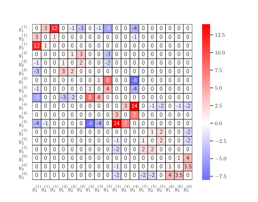
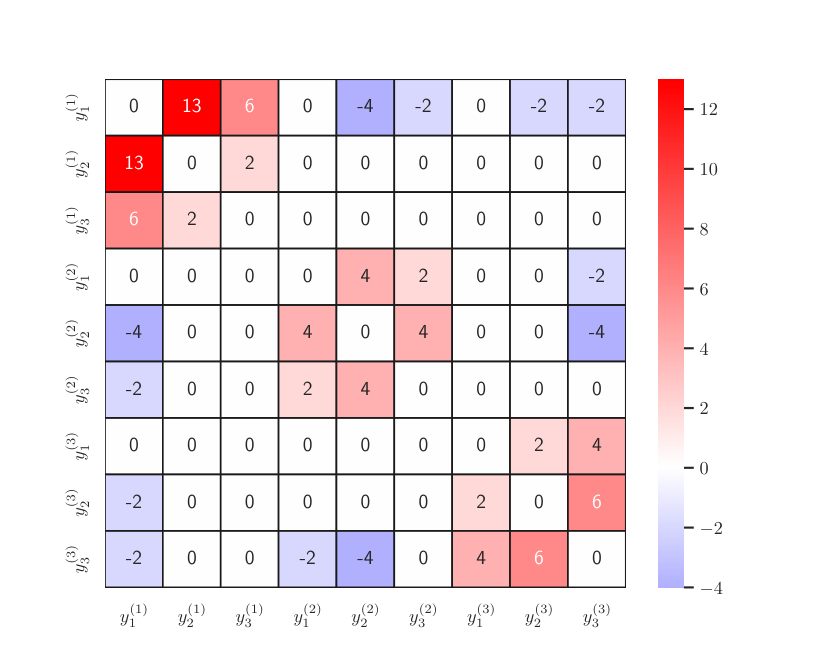
We illustrate the corresponding Hessian matrices as heatmaps in Fig. 1, from which we see clearly a high sparsity in all cases. Moreover, for the second example with n=3n=3 points in 3-D objective space, as predicted by Theorem 3, we obtain exactly 12​n−612n-6 (=30)(=30) positive components. Also, we have verified the above computation by comparing the results obtained from Python, Mathematica, and automatic differentiation performed in our previous work [WED+22].

Refer to caption
(a) Example 1
Refer to caption
(b) Example 2
Refer to caption
(c) Example 3
Refer to caption
(d) Example 4
Figure 1: The hypervolume Hessian matrix ∂2ℋ/∂𝐘​∂𝐘⊤\partial^{2}\mathcal{H}/\partial\mathbf{Y}\partial\mathbf{Y}^{\top} w.r.t. objective vectors rendered as heatmaps for three examples given in Sec. 5.

6 Discussion and Outlook

This paper highlights two approaches for computing the components of the Hessian matrix of the hypervolume indicator HV\operatorname{HV} of a multi-set of points in objective space and of a multi-set of points in the decision space ℋ𝐅\mathcal{H}_{\mathbf{F}}. The approach of set-scalarization, as originated in [EDB07, ED12] for the gradient of the hypervolume indicator. The main results of the paper are as follows:

  1. 1.

    the hypervolume indicator of ℋ𝐅\mathcal{H}_{\mathbf{F}} can now be computed analytically not only for the bi-objective case as in [SSW+20], but also for more than two objective functions (Theorem 1).

  2. 2.

    the time complexity of computing all non-zero components of the 3-D hypervolume indicator HV\operatorname{HV} for vectorized sets 𝐘\mathbf{Y} with nn points in general position is in Θ⁡(n​log⁡n)\Theta(n\log n). (Theorem 2)

  3. 3.

    The number of non-zero components of the Hessian matrix is at most 12​n−612n-6. The space complexity of the Hessian matrix computation and the space required to store all components is in O⁡(n)O(n). (Theorem 3).

  4. 4.

    it holds that ∂ℋ/∂yk\partial\mathcal{H}/\partial y_{k} is always the hypervolume contribution of the projection of yky_{k} along axis kk. (Theorem 4).

  5. 5.

    the analytical computation of the higher derivatives of the mm-dimensional hypervolume indicator HV\operatorname{HV} for m>1m>1can be formulated by computing the gradient of the gradient, which can be essentially achieved by the recursive application of Theorem (Theorem 4) (computing the m−2m-2-dimensional projection’s contributions along the yky_{k} axis, of the m−1m-1 dimensional projections’ hypervolume contributions along the yky_{k}); and taking special care of the role of the reference points and signs of non-zero components as detailed in Alg. 2.

Some interesting next steps would be to

  1. 1.

    investigate the rank of the Hypervolume Hessian matrix and its numerical stability of second-order methods that use the Hessian matrix of ℋ𝐅\mathcal{H}_{\mathbf{F}} (or its inverse) in their iteration, such as the Hypervolume Newton Method [SHSE14, SSW+20].

  2. 2.

    find (asymptotically) efficient algorithms for the computation of the higher-order derivative tensors and for more than three-dimensional cases. The latter might, however, find the asymptotical time complexity of the N-D Hessian matrix computation might turn out to be a difficult endeavor, as it is not even known what the asymptotical time complexity of HV\operatorname{HV} is. What is more promising is to bound the number of the non-zero components in the Hessian matrix, which is related to the number of n−2n-2 dimensional facets in the ortho-convex polyhedron that marks the measured region of HV\operatorname{HV}. It is conjectured that in the mm-dimensional case, it also grows linearly in nn (the number of points in the approximation set) but exponentially in mm (the number of objectives). However, dimension sweep algorithms also yield high efficiency in the 4-D case and can probably be easily adapted [GFE+12].

More generally, it is remarked that besides the hypervolume indicator also, other measures have been proposed for the quality of Pareto front approximations, such as the inverted generational distance [IMN15] or the averaged Hausdorff distance [SDMCC+16, UBV+20], with sometimes advantageous properties regarding the uniformity the point distributions in their maximum. Also, for those, the approach of vectorization of the input set is promising, and the analytical computation and subsequent analysis of the Hessian matrix can be an interesting approach. The code for computing analytically the Hessian matrix of HV\operatorname{HV} has been validated on example data and made available in a GitHub repository.22 2 https://github.com/wangronin/HypervolumeDerivatives The repository includes an implementation based on Alg. 2 in Python and in Mathematica, as well as the data of the examples.

Remark: The authors have been listed alphabetically in this paper, and all authors have contributed to the completion of the manuscript.
Author contributions: HW + ME + AD: Concept and formulation of the general analytical expression for the matrix, ME: 3-D Dimension sweep algorithm and 3-D Complexity Analysis; AD+HW: Improved mathematical notation and numerical validation experiments; HW: theoretical analysis of the general N-dimensional Hessian matrix; All authors: General set-vectorization concepts, motivation, revision/editing of formulation of the paper.

References

  • [BNE07] Nicola Beume, Boris Naujoks, and Michael T. M. Emmerich. SMS-EMOA: multiobjective selection based on dominated hypervolume. Eur. J. Oper. Res., 181(3):1653–1669, 2007.
  • [DD02] Emmanuele DiBenedetto and Emmanuele Debenedetto. Real analysis. Springer, 2002.
  • [ED12] Michael Emmerich and André H. Deutz. Time Complexity and Zeros of the Hypervolume Indicator Gradient Field. In Oliver Schuetze, Carlos A. Coello Coello, Alexandru-Adrian Tantar, Emilia Tantar, Pascal Bouvry, Pierre Del Moral, and Pierrick Legrand, editors, EVOLVE - A Bridge between Probability, Set Oriented Numerics, and Evolutionary Computation III [EVOLVE 2012, Mexico City, Mexico, August 7-9, 2012, selection of extended papers], volume 500 of Studies in Computational Intelligence, pages 169–193. Springer, 2012.
  • [EDB07] Michael Emmerich, André Deutz, and Nicola Beume. Gradient-based/evolutionary relay hybrid for computing pareto front approximations maximizing the s-metric. In Thomas Bartz-Beielstein, María José Blesa Aguilera, Christian Blum, Boris Naujoks, Andrea Roli, Günter Rudolph, and Michael Sampels, editors, Hybrid Metaheuristics, pages 140–156, Berlin, Heidelberg, 2007. Springer Berlin Heidelberg.
  • [EYD+16] Michael Emmerich, Kaifeng Yang, André H. Deutz, Hao Wang, and Carlos M. Fonseca. A Multicriteria Generalization of Bayesian Global Optimization. In Panos M. Pardalos, Anatoly Zhigljavsky, and Julius Zilinskas, editors, Advances in Stochastic and Deterministic Global Optimization, volume 107 of Springer Optimization and Its Applications, pages 229–242. Springer, 2016.
  • [GFE+12] Andreia P Guerreiro, Carlos M Fonseca, Michael TM Emmerich, et al. A fast dimension-sweep algorithm for the hypervolume indicator in four dimensions. In CCCG, pages 77–82, 2012.
  • [IMN15] Hisao Ishibuchi, Hiroyuki Masuda, and Yusuke Nojima. A study on performance evaluation ability of a modified inverted generational distance indicator. New York, NY, USA, 2015. Association for Computing Machinery.
  • [KLP75] H. T. Kung, Fabrizio Luccio, and Franco P. Preparata. On Finding the Maxima of a Set of Vectors. J. ACM, 22(4):469–476, 1975.
  • [PSSL22] Luís Paquete, Britta Schulze, Michael Stiglmayr, and Ana C Lourenço. Computing representations using hypervolume scalarizations. Computers & Operations Research, 137:105349, 2022.
  • [SDMCC+16] Oliver Schütze, Christian Domínguez-Medina, Nareli Cruz-Cortés, Luis Gerardo de la Fraga, Jian-Qiao Sun, Gregorio Toscano, and Ricardo Landa. A scalar optimization approach for averaged Hausdorff approximations of the Pareto front. Engineering Optimization, 48(9):1593–1617, 2016.
  • [SHSE14] Victor Adrián Sosa Hernández, Oliver Schütze, and Michael Emmerich. Hypervolume maximization via set based newton’s method. In EVOLVE-a bridge between probability, set oriented numerics, and evolutionary computation V, pages 15–28. Springer, 2014.
  • [SSW+20] Víctor Adrián Sosa-Hernández, Oliver Schütze, Hao Wang, André H. Deutz, and Michael Emmerich. The Set-Based Hypervolume Newton Method for Bi-Objective Optimization. IEEE Trans. Cybern., 50(5):2186–2196, 2020.
  • [UBV+20] Lourdes Uribe, Johan M Bogoya, Andrés Vargas, Adriana Lara, Günter Rudolph, and Oliver Schütze. A set based newton method for the averaged hausdorff distance for multi-objective reference set problems. Mathematics, 8(10):1822, 2020.
  • [WDBE17] Hao Wang, André H. Deutz, Thomas Bäck, and Michael Emmerich. Hypervolume Indicator Gradient Ascent Multi-objective Optimization. In Heike Trautmann, Günter Rudolph, Kathrin Klamroth, Oliver Schütze, Margaret M. Wiecek, Yaochu Jin, and Christian Grimme, editors, Evolutionary Multi-Criterion Optimization - 9th International Conference, EMO 2017, Münster, Germany, March 19-22, 2017, Proceedings, volume 10173 of Lecture Notes in Computer Science, pages 654–669. Springer, 2017.
  • [WED+22] Hao Wang, Michael Emmerich, André Deutz, Víctor A.S. Hernández, and Oliver Schütze. The Hypervolume Newton Method for Constrained Multi-objective Optimization Problems. Preprints, 2022.
  • [ZT98] Eckart Zitzler and Lothar Thiele. Multiobjective Optimization Using Evolutionary Algorithms - A Comparative Case Study. In A. E. Eiben, Thomas Bäck, Marc Schoenauer, and Hans-Paul Schwefel, editors, Parallel Problem Solving from Nature - PPSN V, 5th International Conference, Amsterdam, The Netherlands, September 27-30, 1998, Proceedings, volume 1498 of Lecture Notes in Computer Science, pages 292–304. Springer, 1998.
  • [ZTL+03] Eckart Zitzler, Lothar Thiele, Marco Laumanns, Carlos M. Fonseca, and Viviane Grunert da Fonseca. Performance assessment of multiobjective optimizers: an analysis and review. IEEE Trans. Evol. Comput., 7(2):117–132, 2003.