跳到论文正文
W Papers独立论文阅读器 arXiv:2211.04158 论文正文 计算阅读时间 · 0%
引用这篇论文根据当前论文元数据生成,正式投稿前建议核对。


License: CC BY 4.0
arXiv:2211.04158v2 [math.PR] 27 May 2025

Many-Server Queueing Systems with Heterogeneous Strategic Servers in Heavy Traffic

Burak Büke    Gonçalo dos Reis    Vadim Platonov
a School of Mathematics, University of Edinburgh, The King’s Buildings, Edinburgh, UK
b Centro de Matemática e Aplicaço~\tilde{\text{o}}es (CMA), FCT, UNL, Portugal
\longdateAugust 11, 2026 (\currenttime)
Abstract

In most service systems, the servers are humans who desire to experience a certain level of idleness. In call centers, this manifests itself as the call avoidance behavior, where servers strategically adjust their service rate to strike a balance between the idleness they receive and effort to work harder. Moreover, being humans, each server values this trade-off differently and has different capabilities. Drawing ideas from mean-field game theory, we develop a novel framework, relying on measure-valued processes, to simultaneously address strategic server behavior and inherent server heterogeneity in service systems. This framework enables us to extend the literature on strategic servers in four new directions by: (i) incorporating individual choices of servers, (ii) incorporating individual abilities of servers, (iii) modeling the discomfort experienced by servers due to low levels of idleness, and (iv) considering more general routing policies. Using our framework, we are able to asymptotically characterize asymmetric Nash equilibria for many-server systems with strategic servers.

In simpler cases, it has been shown that the purely quality-driven regime is asymptotically optimal when the servers are strategic. However, we show that if the discomfort increases fast enough as the idleness approaches zero, the quality-and-efficiency-driven regime and other quality driven regimes can be optimal. This is the first time this conclusion appears in the literature.

Keywords: Many-server queues, strategic servers, measure-valued processes, mean field games

2010 AMS subject classifications:
Primary: 90B22, 60F17, 91A15 Secondary: 60K25

1 Introduction

The design and optimization of many-server service systems has been the subject of vigorous research in the last two decades due to the economic importance of these systems and the challenging problems underpinning them. With a worldwide market size of $339.4 billion in 2020 and an expected market size of $500 billion by 2027, call centers constitute a perfect example of these systems [35]. Around 76% of these call centers serve institutions that generate revenues above $250 million/year and more than 13% serve institutions with an annual revenue of $25 billion [17]. Hence, it is no surprise that a small improvement in the service time can lead to millions of dollars in savings [19].

Despite the rapid technological developments, 82% of the US and 74% of the non-US customers want more human interaction [33] and the vast majority of the interactions in call centers are carried out by human agents (servers). The presence of this human factor poses interesting modeling challenges. One such challenge involves ensuring that agents experience adequate idle time between calls to prevent burnout and maintain high motivation levels. Failure to provide these idle times yields in servers strategically slowing down their service in order to create additional idle time – this is generally referred as call avoidance behavior [22]. For example, servers might choose to delay pressing the terminate call button when a call ends or is transferred, and in systems where the call is routed to the server that has been available for longest, servers can become unavailable for a short period of time to put themselves at the end of the list see e.g. [14]. As a more extreme example of this behavior, [18] observe that a significant number of calls last nearly zero seconds, which indicates that some servers are strategically hanging up on the customers to create extra idle time.

Starting with [23], there has been an increasing research interest in modeling many-server systems with strategic servers to determine incentives for servers to work faster. The main stream of work concentrates on the analysis of Markovian queues and aims to analyze equilibria using the stationary probabilities. Hence, the characterization of the stationary probabilities constitutes a key step in this analysis. To the best of our knowledge, the only existing result in this direction is in [25], where the stationary probabilities for systems with heterogeneous servers is provided under a random routing policy where the customers are routed to an idle server chosen uniformly at random. Unfortunately, even for this special case, the equations for the stationary probabilities are extremely involved, rendering an exact analysis of the general case intractable. As a result, the recent work on strategic servers mainly concentrates on identifying symmetric equilibria by setting all service rates equal except for the rate of a tagged server.

Furthermore, beyond strategic behavior, another consequence of servers being humans is the presence of inherent individual differences and preferences among servers. Each server possesses unique capabilities in serving customers, values idle time differently and, at equilibria, one expects each server to serve with a different rate if such equilibrium exists. It is then crucial for the next generation of models to capture these behaviors and analyze the so-called asymmetric equilibria in which servers serve with heterogeneous rates.

The key step in the analysis of asymmetric equilibria is identifying how idleness is distributed among servers featuring heterogeneous service rates, which heavily depends on the routing policy used by the call center. In a recent paper, [11] propose the use of a measure-valued process, referred to as the fairness process, to capture the individual differences in service rates as a means to obtain access to the distribution of server idleness under a given routing policy. [11] prove that in a modified version of Halfin-Whitt scaling [27], the sequence of fairness processes is tight and converges in probability to a constant deterministic process for some common routing policies. Then, they use the fairness process to prove diffusion limits for many-server systems with heterogeneous servers. In this work, we use the fairness process as our main technical tool to analyze many-server systems with strategic heterogeneous servers.

The literature from human resource management indicates that the perception of fairness has a significant effect on employee performance [16, 15]. The distribution of idleness among servers is generally perceived as a measure of fairness. An interesting question regarding the distribution of idleness is whether one can design routing policies in order to distribute the idleness among servers according to servers’ service rates in a pre-specified manner. For example, it is well-known that if the fastest-server-first policy is employed, i.e., the customers are routed to the idle server with the highest service rate, only the slowest servers experience idleness [3, 6, 11]. As another example, [11] show that if customers are routed using a class of policies called totally blind policies, where the server to which a customer is routed is asymptotically independent of the service rate of that server, then the cumulative idleness servers receive is proportional to their service rate. Totally blind policies include longest-idle-server-first, where customers are routed to the server that has been available the longest, and random routing as studied in [25]. Several routing policies have been designed in the literature for service systems with pools of servers to ensure that each pool asymptotically receives a certain proportion of idleness [3, 5, 2, 26, 34, 36]. However, to the best of our knowledge, the question of how to design policies to distribute idleness on an individual server level remains an open problem.

1.1 Our Contributions

Our aim is to push the frontier for the analysis of service systems with strategic servers. Our contributions can be described under two major headings.

Technical Contributions

  1. 1.

    A General Framework to Study Heterogeneous Strategic Servers. In this paper, we introduce a novel framework to study systems with strategic servers and extend the results in four major directions. First, we suggest a utility function to model the individual preferences of servers regarding the trade-off between utility of idleness and cost of working faster. Second, we address the inherent differences between the abilities of servers using random individual maximum and minimum attainable service rates. Third, we model the contribution of percentage of idleness as a concave increasing function of idleness, which we refer as the utility of idleness function to better reflect the marginal benefit of idleness and allows us to model the discomfort experienced by the servers. Finally, we characterize the Nash equilibria for service rate distribution under a more general class of routing policies.

  2. 2.

    Service Systems with Heterogeneity in Quality-Driven Regimes. In Section 4, we provide fluid limits for many-server queues with heterogeneous service rates in quality-driven regimes. A key question regarding fluid and diffusion approximations is whether these approximations can be used to study the stationary behavior of the systems, which require an interchange of limits argument. We prove that this is indeed the case for both quality- and quality-and-efficiency driven regimes.

  3. 3.

    Analysis of Generalized Random Routing Policies. The random routing policy, where an incoming job is assigned to one of the idle servers uniformly at random, is well-understood. However, to the best of our knowledge, there are no results in the literature where incoming customers are randomly assigned to servers with probabilities that depend on the service rates. In Section 5, we present a detailed asymptotical analysis of generalized random routing policies where the routing probabilities can be a function of the service rate and characterize the distribution of idleness among servers with heterogeneous rates under these policies in a quality-driven system. Moreover, using another interchange of limits argument, we also show that this result can also be used to characterize the long run percentage a server with a given service rate is idle.

Practical Contributions and Managerial Insights

  1. 1.

    Fair Distribution of Idleness Among Individual Servers in a Quality-Driven Regime. In the quality-and-efficiency-driven regime, it is possible to design routing policies to attain any pre-specified distribution of idleness among server pools [5, 2, 34, 36]. We show that in the quality-driven regime, where the safety staffing scales linearly with the offered load, this result no longer holds and it may not be possible to design routing policies to attain certain idleness distributions. We characterize necessary conditions for an idleness distribution to be attainable and also prove that the ‘strict inequality’ versions of these conditions are also sufficient by designing general random routing policies to attain the desired distribution of idleness. Moreover, we show that one can use these policies to distribute idleness at an individual server level.

  2. 2.

    The Relationship Between the Optimal Staffing Regime and Servers’ Sensitivity to Idleness. When the servers are homogeneous and idleness contributes to the utility as itself, i.e., the utility of the idleness function is identity, [23] prove that it is optimal to scale the safety staffing linearly with the offered load. In Theorem 6.2, we prove that the main factor in establishing this result is the sensitivity of servers to low levels of idleness, which can be expressed in terms of the derivative of the utility of idleness function near zero and extend the optimality result to a more general class of functions. Moreover, we show that if the servers are sufficiently sensitive to low levels of idleness, then it is asymptotically optimal to adopt a quality-and-efficiency-driven regime.

  3. 3.

    Characterization of the Equilibrium Service Rate Distribution. When servers are heterogeneous and strategic, a central practical question concerns how the equilibrium service rate distribution is influenced by primitive model assumptions. In Section 6.2, we use our framework to derive an equation that characterizes the equilibrium service rate distribution under any generalized random routing policy. Through numerical experiments, we demonstrate that our general framework is very effective in estimating the equilibrium service rate for large many-server systems. Moreover, we present an extensive numerical study to understand how various model parameters affect the shape and scale of the equilibrium service rate distribution.

1.2 Notation

In this work, we assume that all the stochastic processes and the random variables lie in the probability space (Ω,ℱ,ℙ)(\Omega,\mathcal{F},\mathbb{P}). We use the shorthand notation ‘w.p. 1’ instead of ‘with probability 1’ with respect to ℙ\mathbb{P}. We denote the set of real numbers, set of positive real numbers and the positive integers as ℝ,ℝ+\mathbb{R},\mathbb{R}_{+} and ℕ\mathbb{N}, respectively and use ℬ⁡(ℝ+)\mathcal{B}(\mathbb{R}_{+}) to denote the Borel σ\sigma-algebra on ℝ+\mathbb{R}_{+}. We use →\to, →p\stackrel{{\scriptstyle p}}{{\rightarrow}} and ⇒\Rightarrow to denote convergence in ℝ\mathbb{R}, convergence in probability and convergence in measure, respectively. To emphasize that a certain system parameter xx is random, we use the ’∼\sim’ notation as x~\tilde{x}. Also, we define (x)+:=max⁡{x,0}(x)^{+}:=\max\{x,0\} and (x)−:=max⁡{0,−x}(x)^{-}:=\max\{0,-x\}. We define ℂ[α,β]b[0,∞)\mathbb{C}_{[\alpha,\beta]}^{b}[0,\infty) to be the set of continuous bounded functions defined on the interval [α,β][\alpha,\beta], ι⁡(⋅)\iota(\cdot) to be the identity function and 𝕀\mathbb{I} to be the indicator function where 𝕀⁡(A)\mathbb{I}(A) is 1 if AA holds and 00 otherwise. The spaces of right-continuous functions and left-continuous functions are endowed with the Skorokhod-J1J_{1} topology. For any measure η\eta, ⟨f,η⟩:=∫f⁡(x)​𝑑η​(x)\langle f,\eta\rangle:=\int f(x)d\eta(x), and hence, if η\eta is a probability measure ⟨ι,η⟩\langle\iota,\eta\rangle denotes the first moment of η\eta. With a slight abuse of notation, we use FF to denote both the law and the cumulative distribution of random variable, i.e., F⁡(A)F(A) denotes the probability of set AA and F(a)=F((−∞,a])F(a)=F((-\infty,a]) for any real argument aa. We also denote the Dirac measure which assigns a unit measure to point xx as δx​(⋅)\delta_{x}(\cdot). Finally, for any stochastic process X⁡(t)X(t), we use X⁡(∞)X(\infty) to denote a random variable distributed with its stationary distribution. For measure-valued processes, we find that it is more appropriate to use ηt\eta_{t} and η∞\eta_{\infty} notation instead of η⁡(t)\eta(t) and η⁡(∞)\eta(\infty).

2 Literature on Strategic Behavior in Queues

The vast majority of the literature on queues with strategic players concentrates on the strategic behavior of customers while joining a queue. We refer the reader to the excellent monographs [28] and [29] for an extensive review of the literature on strategic customers. Motivated by the competition between two firms, two-server queues with strategic servers has also received attention in the literature see, e.g. [31, 21, 12, 13]. More recently, [1] extend this line of research to cover multiple firms each of which are operating as M/M/NM/M/N queues.

The study of servers who are behaving strategically within the same organization is relatively recent and to the best of our knowledge started with the seminal work of [23]. They assume that the servers (agents) are identically sensitive to the idleness they receive and there is a non-cooperative game between servers to set their service rates in order to maximize their utility which is defined as a combination of the server’s idle time and effort to speed up the service. The system operator routes the customers to the servers with the aim of incentivizing servers using the idleness experienced – they refer to this as incentive-aware routing. In an M/M/NM/M/N queue setting, they show the existence of symmetric equilibrium under policies which route customers to servers according to their idle time. To solve the problem, [23] explicitly assume that the servers need to choose service rates in a way that ensures system stability. [4] show that this assumption is not necessary using Tarski’s intersection theorem. [24] studies the above results comparing queueing systems with pooled and dedicated queues under r-routing policies, a class of randomized policies which routes the customers to servers randomly with probabilities proportional to the rrth power of the service rate. He provides analytical results for systems with dedicated queues, but due to their complexity he only studies the pooled queues numerically. One of the major contributions of our work is to provide analytical tools for the asymptotic study of pooled queues. In addition to incentive-aware routing, one can also provide monetary incentives based on the service speed. [37] characterize a joint routing and payment policy to optimize performance under the assumption that there is a trade-off between service speed and service quality. [38] analyze equilibrium in loss systems with finite buffer capacity when both incentive-aware routing and payment incentives are used. An interesting recent work by [7] uses mean-field games ideas to study strategic servers with dedicated queues and designs a dynamic arrival rate control policy. To the best of our knowledge, the approach we offer is novel, in particular, for the application of mean-field games to queueing systems.

3 A Many-Server Queueing Model with Strategic and Heterogeneous Servers

We consider a sequence of queueing systems where arrivals at the nnth system follow a Poisson process with rate λn\lambda^{n}. We have the following standard assumption on arrival rates.

Assumption 3.1.

There exists a 0<λ¯<∞0<\bar{\lambda}<\infty such that n−1/2(λn−nλ¯)→0n^{-1/2}(\lambda^{n}-n\bar{\lambda})\to 0 as n→∞n\to\infty.

If there are idle servers upon the arrival of a customer, the customer is routed to one of these servers according to a prespecified routing policy π\pi. All servers in the system have the skills to serve any arriving customer, albeit with different rates. If all servers are busy, the customer waits in a queue. Customers are impatient with exponential(γ\gamma) patience times, independent of other customers. If the patience time of a customer expires before the service commences, the customer abandons the system. Once the service commences, the customer only departs when the service finishes. We assume that customers are served on a first-come-first-served basis.

For the system outlined above, the system operator decides on the routing policy π\pi and the staffing level. The routing policy determines how idleness is distributed among servers with different rates. At this point, we only assume that the routing policy is non-idling, i.e., there can only be customers in the queue if all the servers in the system are busy.

Due to the non-cooperative game between servers, there is a circular relationship between staffing level and individual service rates. The staffing level is determined by the expected service rate, and the distribution of service rates is determined by the idleness experienced by each server with different rate, the latter being directly influenced by the staffing level and the routing policy. Our main goal in this work is to identify whether equilibria exist and characterize any equilibrium given the system operator’s staffing and routing policies. As the servers differ individually in terms of their capabilities and preferences, the resulting equilibria will be asymmetric, in general.

The system operator aims to set the staffing level to be the offered load (the minimum number of staff required to stabilize the system if there were no abandonments), and a safety staffing proportional to a power α\alpha of the offered load, where 1/2≤α≤11/2\leq\alpha\leq 1, to achieve a certain quality of service. Suppose that the server kk in the nnth system serves with rate μ~kn\tilde{\mu}_{k}^{n}. If the system operator knows the distribution of these service rates to be FF with an expected value μ¯F\bar{\mu}_{F}, she sets the staffing level for the nnth system to be

Nαn=λnμ¯F+β​(λnμ¯F)α,N_{\alpha}^{n}=\frac{\lambda^{n}}{\bar{\mu}_{F}}+\beta\left(\frac{\lambda^{n}}{\bar{\mu}_{F}}\right)^{\alpha}, (3.1)

where β>0\beta>0 see, e.g., [18]. Following the classification in [20], we say that the system operates in a quality-driven (QD) regime when 1/2<α≤11/2<\alpha\leq 1 and in a quality-and-efficiency-driven (QED) regime when α=1/2\alpha=1/2. In the literature, it is quite common to restrict the quality-driven regime to the case with α=1\alpha=1 and this case also plays a major role in our study. Hence, to differentiate, we say that the system operates in a purely quality-driven regime if α=1\alpha=1. The system operator sets the staffing parameters, α,β\alpha,\beta, and the routing policy π\pi in order to minimize an operating cost, CO​(α,β,π)C_{O}(\alpha,\beta,\pi), which can be expressed as

COn​(α,β,π)=cS​Nαn+cW​λn​𝔼​[Wn​(∞)]+cA​𝔼​[R¯n​(∞)]C_{O}^{n}(\alpha,\beta,\pi)=c_{S}N_{\alpha}^{n}+c_{W}\lambda^{n}\mathbb{E}[W^{n}(\infty)]+c_{A}\mathbb{E}[\bar{R}^{n}(\infty)] (3.2)

where cS,cWc_{S},c_{W} and cAc_{A} are the unit staffing cost, unit queueing time cost per customer and unit abandonment cost, respectively, 𝔼​[Wn​(∞)]\mathbb{E}[W^{n}(\infty)] is the long run average queueing time per customer and 𝔼​[R¯n​(∞)]\mathbb{E}[\bar{R}^{n}(\infty)] is the long run abandonment rate from the system.

On the other hand, each server in the system aims to set her service rate to maximize her own utility, where utility is defined as a trade-off between the expected long run proportion of idleness she experiences and an effort cost she incurs for working faster. This setting is similar to [23] with two fundamental differences. First, we model the contribution of idleness to the utility as a concave increasing function of the long run percentage idleness experienced rather than the long run percentage idleness itself. In addition to modeling the decreasing marginal return of idleness, this approach also helps us model the situations where working without any breaks is unacceptable to the servers. Second, we model the trade-off between ‘benefits of idleness’ and ‘effort cost’ to be server specific by introducing a multiplicative random coefficient to the effort cost function. The idleness each server experiences depends ultimately on the service rates of all servers in the system. Letting Ikn​(t)I_{k}^{n}(t) to be the idleness process of server kk, where Ikn​(t)I_{k}^{n}(t) takes the value 11 if the server kk in system nn is idle at time tt and is 00 otherwise, we define the utility function of server kk in the nnth system, serving with rate μ\mu, to be

Ukn​(μ,F)=uI​(𝔼⁡[Ikn​(∞)|μ~kn=μ])−a~kn​c​(μ),U_{k}^{n}(\mu,F)=u_{I}\big(\mathbb{E}[I_{k}^{n}(\infty)|\tilde{\mu}_{k}^{n}=\mu]\big)-\tilde{a}_{k}^{n}c(\mu), (3.3)

where FF is the distribution of individual service rates and determines the expected stationary idleness of the given server. We refer to uI​(⋅)u_{I}(\cdot) as the utility of idleness function and assume it to be concave and increasing. The effort cost function, c⁡(⋅)c(\cdot), is assumed to be convex and increasing. We also assume that both uI​(⋅)u_{I}(\cdot) and c⁡(⋅)c(\cdot) are twice continuously differentiable. The coefficient a~kn\tilde{a}_{k}^{n} is a positive random variable with distribution Fa​(⋅)F_{a}(\cdot) and determines the personal preference of server kk in regards to the trade-off between utility of idleness and the effort cost and use fa​(⋅)f_{a}(\cdot) to denote the density function of a~kn\tilde{a}_{k}^{n} when it is a continuous random variable. We assume that each server kk deterministically knows her trade-off parameter a~kn\tilde{a}_{k}^{n}.

Each server kk in the nnth system has an inherent minimum service rate, μ~min,kn\tilde{\mu}_{{\min},k}^{n}, which the server can achieve with minimal effort and an inherent maximum achievable service rate, μ~max,kn\tilde{\mu}_{{\max},k}^{n}, which the server cannot improve upon by working faster regardless of how much effort she puts into her work. The system operator does not have prior information about these individual minimum and maximum rates and hence, they are modeled as random variables following a common joint distribution Fmin,maxF_{\min,\max} with marginals FminF_{\min} and FmaxF_{\max}. We assume that these individual minimum and maximum service rates are uniformly bounded, i.e., there exists μmin\mu_{\min} and μmax\mu_{\max} such that

0<μmin≤μ~min,kn≤μ~kn≤μ~max,kn≤μmax<∞, for all ​k,n∈ℕ w.p. ​1.0<\mu_{\min}\leq\tilde{\mu}_{\min,k}^{n}\leq\tilde{\mu}_{k}^{n}\leq\tilde{\mu}_{\max,k}^{n}\leq\mu_{\max}<\infty,\quad\mbox{ for all }k,n\in\mathbb{N}\quad\mbox{ w.p. }1. (3.4)

We also assume independence among vectors (a~kn,μ~min,kn,μ~max,kn)(\tilde{a}_{k}^{n},\tilde{\mu}_{\min,k}^{n},\tilde{\mu}_{\max,k}^{n}) for each kk.

Given a distribution F(0)F^{(0)} for the service rates and the system operator’s decisions on α,β\alpha,\beta and π\pi, each server kk in the nnth system serves with the service rate μ~kn\tilde{\mu}_{k}^{n} that maximizes her utility, i.e.,

μ~kn∈arg​maxμ∈[μ~min,kn,μ~max,kn]⁡Ukn​(μ,F(0)).\tilde{\mu}_{k}^{n}\in\argmax_{\mu\in[\tilde{\mu}_{{\min},k}^{n},\tilde{\mu}_{{\max},k}^{n}]}U_{k}^{n}(\mu,F^{(0)}). (3.5)

As a~kn,μ~min,kn\tilde{a}_{k}^{n},\tilde{\mu}_{{\min},k}^{n} and μ~max,kn\tilde{\mu}_{{\max},k}^{n} are random and only known by server kk, the resulting service rate is random and the distributions of these parameters determine the distribution F(1)F^{(1)} of the optimal service rates. Our goal in this work is to study the equilibrium service rate distribution FF by characterizing the fixed point where F(0)=F(1)=FF^{(0)}=F^{(1)}=F, based on the given values of α,β\alpha,\beta and π\pi. Our analysis also provides important insights on the optimal regime parameter α\alpha for the system operator.

3.1 Dynamics of the System Processes

In this section, we define the stochastic processes in our model. We denote the number of customers in the nnth system at time tt as Xn​(t)X^{n}(t). For the nnth system, the arrival process is a Poisson process with rate λn\lambda^{n} and An​(t)A^{n}(t) denotes the number of arrivals by time tt. The service time of a customer depends on the server and takes an exponential time with rate μ~kn\tilde{\mu}_{k}^{n} if the customer is served by server kk. In this section, we assume that the service rates μ~kn,1≤k≤Nαn\tilde{\mu}_{k}^{n},1\leq k\leq N_{\alpha}^{n}, are i.i.d. random variables with a common known distribution FF having mean μ¯F\bar{\mu}_{F} and variance σF2\sigma_{F}^{2}. In Section 6, we analyze in detail how this distribution is determined as a result of the strategic decisions of the servers. The departure process for server kk and the number of abandonments by time tt is denoted Dkn​(t)D_{k}^{n}(t) and R0n​(t)R_{0}^{n}(t), respectively. We have the following balance equation for the system length process Xn​(t)X^{n}(t),

Xn​(t)=Xn​(0)+An​(t)−∑k=1NαnDkn​(t)−R0n​(t), for all ​t≥0,n∈ℕ.X^{n}(t)=X^{n}(0)+A^{n}(t)-\sum_{k=1}^{N_{\alpha}^{n}}D_{k}^{n}(t)-R_{0}^{n}(t),\quad\mbox{ for all }t\geq 0,\ n\in\mathbb{N}. (3.6)

Taking Skn​(t)S_{k}^{n}(t) and Rn​(t)R^{n}(t) as independent unit rate Poisson processes for all kk and nn, we can equivalently define the departure and the abandonment processes as

Dkn​(t):=Skn​(μ~kn​∫0t(1−Ikn​(s))​𝑑s)andR0n​(t):=Rn​(γ​∫0t(Xn​(s)−Nαn)+​𝑑s),D_{k}^{n}(t):=S_{k}^{n}\left(\tilde{\mu}_{k}^{n}\int_{0}^{t}\big(1-I_{k}^{n}(s)\big)ds\right)\quad\mbox{and}\quad R_{0}^{n}(t):=R^{n}\left(\gamma\int_{0}^{t}\big(X^{n}(s)-N^{n}_{\alpha}\big)^{+}ds\right),

and can write (3.6) as

Xn​(t)=Xn​(0)+An​(t)−∑k=1NαnSkn​(μ~kn​∫0t(1−Ikn​(s))​𝑑s)−Rn​(γ​∫0t(Xn​(s)−Nαn)+​𝑑s),X^{n}(t)=X^{n}(0)+A^{n}(t)-\sum_{k=1}^{N_{\alpha}^{n}}S_{k}^{n}\left(\tilde{\mu}_{k}^{n}\int_{0}^{t}\big(1-I_{k}^{n}(s)\big)ds\right)-R^{n}\left(\gamma\int_{0}^{t}\big(X^{n}(s)-N^{n}_{\alpha}\big)^{+}ds\right), (3.7)

for all t≥0,n∈ℕt\geq 0,n\in\mathbb{N}. The non-idling property of the routing policy implies

(Xn​(t)−Nαn)−=∑k=1NαnIkn​(t), for all ​t≥0,n∈ℕ.\left(X^{n}(t)-N^{n}_{\alpha}\right)^{-}=\sum_{k=1}^{N_{\alpha}^{n}}I^{n}_{k}(t),\mbox{ for all }t\geq 0,\ n\in\mathbb{N}.

For all 1/2≤α≤11/2\leq\alpha\leq 1, we define the scaled processes X^αn​(t):=n−α​(Xn​(t)−Nαn)\hat{X}_{\alpha}^{n}(t):=n^{-\alpha}(X^{n}(t)-N_{\alpha}^{n}) and I^k,αn​(t):=n−α​Ikn​(t)\hat{I}_{k,\alpha}^{n}(t):=n^{-\alpha}I_{k}^{n}(t). We also use the shorthand notation I^αn​(t):=∑k=1NαnI^k,αn​(t)\hat{I}_{\alpha}^{n}(t):=\sum_{k=1}^{N_{\alpha}^{n}}\hat{I}_{k,\alpha}^{n}(t) for the total scaled idleness in the system. Regarding the initial system length, we make the following assumption.

Assumption 3.2.

The initial system lengths X^αn​(0)\hat{X}_{\alpha}^{n}(0) are uniformly integrable and X^αn​(0)⇒ξ0\hat{X}_{\alpha}^{n}(0)\Rightarrow\xi_{0} as n→∞n\to\infty, where ξ0\xi_{0} is an integrable random variable.

We also have the following assumption on the routing policy.

Assumption 3.3.

Under the routing policy π\pi, for any 0≤k,j≤Nαn0\leq k,j\leq N_{\alpha}^{n} and μ∈[μmin,μmax]\mu\in[\mu_{\min},\mu_{\max}],

𝔼⁡[Ikn​(∞)|μ~kn=μ]=𝔼⁡[Ijn​(∞)|μ~jn=μ].\mathbb{E}[I_{k}^{n}(\infty)|\tilde{\mu}_{k}^{n}=\mu]=\mathbb{E}[I_{j}^{n}(\infty)|\tilde{\mu}_{j}^{n}=\mu].

Assumption 3.3 ensures that the routing policy does not discriminate against any server and all servers working with the same rate are expected to receive the same proportional idleness in the long run. Using symmetry arguments, it can be easily seen that any routing policy which does not explicitly use the server index kk satisfies this assumption.

3.2 The Fairness Process

The utility of a server is defined based on the long run proportion of time the server stays idle. This quantity is difficult to calculate and manipulate, especially when servers are heterogeneous. To be able to analyze this quantity in the heterogeneous setting, we use the fairness process introduced by [11]. In this section, we provide the definition of the fairness process and how it can be used to analyze strategic server behavior.

Defining the empirical distribution of service rates for the nnth system as Fn[μ,μ+Δ):=(Nαn)−1∑j=1Nαnδμjn[μ,μ+Δ) for all μ∈[μmin,μmax] and Δ>0,F^{n}[\mu,\mu+\Delta):=(N_{\alpha}^{n})^{-1}\sum_{j=1}^{N_{\alpha}^{n}}\delta_{\mu_{j}^{n}}[\mu,\mu+\Delta)\mbox{ for all }\mu\in[\mu_{\min},\mu_{\max}]\mbox{ and }\Delta>0, we can write

𝔼⁡[Ikn​(∞)|μ~kn=μ]\displaystyle\mathbb{E}[I_{k}^{n}(\infty)|\tilde{\mu}_{k}^{n}=\mu]
=limt→∞1t​𝔼​[∫0tIkn​(s)​𝑑s|μ~kn=μ]\displaystyle\quad=\lim_{t\to\infty}\frac{1}{t}\mathbb{E}\left[\int_{0}^{t}I_{k}^{n}(s)ds|\tilde{\mu}_{k}^{n}=\mu\right]
=limΔ→0limt→∞1t​𝔼​[∑j=1Nαnδμ~jn[μ,μ+Δ)∫0tIjn(s)dsNαnFn[μ,μ+Δ)|μ~kn=μ]\displaystyle\quad=\lim_{\Delta\to 0}\lim_{t\to\infty}\frac{1}{t}\mathbb{E}\left[\frac{\sum_{j=1}^{N_{\alpha}^{n}}\delta_{\tilde{\mu}_{j}^{n}}[\mu,\mu+\Delta)\int_{0}^{t}I_{j}^{n}(s)ds}{N_{\alpha}^{n}F^{n}[\mu,\mu+\Delta)}\Big|\tilde{\mu}_{k}^{n}=\mu\right]
=limΔ→0limt→∞1t​𝔼​[nαNαnFn[μ,μ+Δ)×∑j=1Nαnδμ~jn[μ,μ+Δ)∫0tI^j,αn(s)ds∫0tI^αn​(s)​𝑑s×∫0tI^αn​(s)​𝑑s|μ~kn=μ].\displaystyle\quad=\lim_{\Delta\to 0}\lim_{t\to\infty}\frac{1}{t}\mathbb{E}\left[\frac{n^{\alpha}}{N_{\alpha}^{n}F^{n}[\mu,\mu+\Delta)}\times\frac{\sum_{j=1}^{N_{\alpha}^{n}}\delta_{\tilde{\mu}_{j}^{n}}[\mu,\mu+\Delta)\int_{0}^{t}\hat{I}_{j,\alpha}^{n}(s)ds}{\int_{0}^{t}\hat{I}_{\alpha}^{n}(s)ds}\times\int_{0}^{t}\hat{I}_{\alpha}^{n}(s)ds\Big|\tilde{\mu}_{k}^{n}=\mu\right]. (3.8)

The second term inside the expectation represents the proportion of total cumulative idleness experienced by servers whose service rates lie between μ\mu and μ+Δ\mu+\Delta. [11] represent the distribution of cumulative idleness among servers with different service rates using a measure-valued process and they coin this process as the fairness process. The name is motivated by the idea that the distribution of idleness is generally viewed as a measure of fairness towards servers see, e.g., [2, 36]. By selecting a specific routing policy, the system operator determines the fairness process, i.e., how idleness is distributed among servers as a function of service effort. For example, a routing policy might aim to distribute idleness equally, reflecting an egalitarian notion of fairness, or reward faster servers with more idleness, representing a performance-based perspective on fairness. In response, servers decide their service rates to maximize their utility as defined in (3.3). Thus, the fairness process corresponding to a routing policy plays a key role in our analysis by shaping the structure of the utility function.

Setting τ0n:=inf{t>0:∫0tI^αn​(s)​𝑑s>0}\tau_{0}^{n}:=\inf\{t>0:\int_{0}^{t}\hat{I}_{\alpha}^{n}(s)ds>0\} as the first time idleness is experienced by the system, the fairness process for the nnth system is defined as

ηα,tπ,n​(𝔸):={∑k=1Nαnδμkn​(𝔸)​∫0tI^k,αn​(s)​𝑑s∫0tI^αn​(s)​𝑑s,if t>τ0n,δ0​(𝔸),if t≤τ0n,\eta_{\alpha,t}^{\pi,n}(\mathbb{A}):=\left\{\begin{array}[]{ll}\displaystyle\frac{\sum_{k=1}^{N_{\alpha}^{n}}\delta_{\mu_{k}^{n}}(\mathbb{A})\int_{0}^{t}\hat{I}_{k,\alpha}^{n}(s)ds}{\int_{0}^{t}\hat{I}_{\alpha}^{n}(s)ds}&,\mbox{if }t>\tau_{0}^{n},\\ \delta_{0}(\mathbb{A})&,\mbox{if }t\leq\tau_{0}^{n},\end{array}\right. (3.9)

for all 𝔸∈ℬ⁡(ℝ+)\mathbb{A}\in\mathcal{B}(\mathbb{R}_{+}), i.e., ηα,tπ,n​(𝔸)\eta_{\alpha,t}^{\pi,n}(\mathbb{A}) represents the proportion of total cumulative idleness received up to time tt by the servers whose service rates lie in set 𝔸\mathbb{A}. To make this quantity well-defined and avoid division by 0, it is set to δ0​(𝔸)\delta_{0}(\mathbb{A}) as a placeholder until the total cumulative idleness in the system is positive. Hence, (3.8) can be written more compactly using the fairness process as

𝔼⁡[Ikn​(∞)|μ~kn=μ]\displaystyle\mathbb{E}[I_{k}^{n}(\infty)|\tilde{\mu}_{k}^{n}=\mu] =limΔ→0limt→∞1t​𝔼​[nαNαn×ηα,tπ,n[μ,μ+Δ)Fn[μ,μ+Δ)×∫0tI^αn​(s)​𝑑s|μ~kn=μ].\displaystyle=\lim_{\Delta\to 0}\lim_{t\to\infty}\frac{1}{t}\mathbb{E}\left[\frac{n^{\alpha}}{N_{\alpha}^{n}}\times\frac{\eta_{\alpha,t}^{\pi,n}[\mu,\mu+\Delta)}{F^{n}[\mu,\mu+\Delta)}\times\int_{0}^{t}\hat{I}_{\alpha}^{n}(s)ds|\tilde{\mu}_{k}^{n}=\mu\right]. (3.10)

Hence, the long run proportion of time a server is idle is determined by the total idleness the system experiences and how this idleness is distributed among servers as a consequence of the routing policy. In the QED regime (α=1/2\alpha=1/2), [11] show that if the limiting fairness process can be characterized for a routing policy, then the limiting behavior of the total cumulative idleness can also be determined, which we extend to QD regimes (1/2<α<11/2<\alpha<1) in Theorem 4.1. Unfortunately, the fairness processes do not converge in measure in any of the four Skorokhod topologies as n→∞n\to\infty and the limiting process should be defined based on shifted versions of the fairness processes. The formal definition of this limit is presented in the Appendix A.2.

[11] observe that under most stationary policies the fairness processes converge on a faster scale than the scaled system length processes. Hence the limiting fairness process does not depend on tt after τ0:=limn→∞τ0n\tau_{0}:=\lim_{n\to\infty}\tau_{0}^{n} and is deterministic, i.e., ηt,απ=ηαπ\eta_{t,\alpha}^{\pi}=\eta_{\alpha}^{\pi} for all t>τ0t>\tau_{0}. For these cases, we refer to ηαπ\eta_{\alpha}^{\pi} as the limiting fairness measure, slightly abusing the terminology. Proposition 3.4 summarizes several findings of [11], extending from α=1/2\alpha=1/2 to 1/2≤α<11/2\leq\alpha<1.

Proposition 3.4.

Suppose 1/2≤α<11/2\leq\alpha<1 and let ηαS​S​F,ηαF​S​F,ηαL​I​S​F\eta_{\alpha}^{SSF},\eta_{\alpha}^{FSF},\eta_{\alpha}^{LISF} and ηαR​R\eta_{\alpha}^{RR} be the limiting fairness processes corresponding to slowest-server-first, fastest-server-first, longest-idle-server-first and uniformly random routing, respectively. Then, for all t>τ0t>\tau_{0} and 𝔸∈ℬ⁡(ℝ+)\mathbb{A}\in\mathcal{B}(\mathbb{R}_{+})

ηα,tS​S​F=δμmax​(𝔸),ηα,tF​S​F=δμmin​(𝔸)​ and ​ηα,tL​I​S​F​(𝔸)=ηα,tR​R​(𝔸)=∫𝔸μ​F​(𝑑μ)∫ℝ+μ​F​(𝑑μ).\displaystyle\eta_{\alpha,t}^{SSF}=\delta_{\mu_{\max}}(\mathbb{A}),\;\eta_{\alpha,t}^{FSF}=\delta_{\mu_{\min}}(\mathbb{A})\;\textrm{ and }\eta_{\alpha,t}^{LISF}(\mathbb{A})=\eta_{\alpha,t}^{RR}(\mathbb{A})=\frac{\int_{\mathbb{A}}\mu F(d\mu)}{\int_{\mathbb{R}_{+}}\mu F(d\mu)}.

Theorem 1 indicates that under the slowest-server-first and fastest-server-first policies, only the fastest and slowest servers, respectively, experience non-negligible idleness and in general cannot be considered fair. However, under both the longest-idle-server-first and uniformly random routing policies, the idleness a server experiences is proportional to her service rate and can be considered fair for some definitions of fairness. Unfortunately, the case with α=1\alpha=1 is far more involved and similar results do not hold as we show in Section 5.

4 Convergence of the Scaled System Length Processes

In this section, we derive fluid and diffusion approximations as the weak limit of the scaled system length processes {X^αn}n∈ℕ\{\hat{X}_{\alpha}^{n}\}_{n\in\mathbb{N}} when 1/2≤α≤11/2\leq\alpha\leq 1 using the fairness process defined in Section 3.2. Recall that X^αn​(0)⇒ξ0\hat{X}_{\alpha}^{n}(0)\Rightarrow\xi_{0} and ⟨ι,ηα,tπ⟩\langle\iota,\eta_{\alpha,t}^{\pi}\rangle corresponds to the first moment of the measure ηα,tπ\eta_{\alpha,t}^{\pi}.

Theorem 4.1.

Suppose that the limiting fairness process under the adopted routing policy π\pi is ηα,tπ\eta_{\alpha,t}^{\pi}. Then, X^αn⇒ξα\hat{X}_{\alpha}^{n}\Rightarrow\xi_{\alpha} as n→∞n\to\infty, where

  1. 1.

    if α=1/2\alpha=1/2, ξ1/2\xi_{1/2} is the strong solution to the stochastic differential equation

    ξ1/2​(t)=ξ0+(2​λ¯)1/2​W​(t)−(βF​(λ¯​μ¯F)1/2+ζ)​t+⟨ι,η1/2,tπ⟩​∫0t(ξ1/2​(s))−​𝑑s−γ​∫0t(ξ1/2​(s))+​𝑑s,\xi_{1/2}(t)=\xi_{0}+(2\bar{\lambda})^{1/2}W(t)-\left(\beta_{F}(\bar{\lambda}\bar{\mu}_{F})^{1/2}+\zeta\right)t+\langle\iota,\eta_{1/2,t}^{\pi}\rangle\int_{0}^{t}(\xi_{1/2}(s))^{-}ds-\gamma\int_{0}^{t}(\xi_{1/2}(s))^{+}ds, (4.1)

    for all t≥0t\geq 0 where ζ∼\zeta\sim Normal​(0,σF2​λ¯α​μ¯F−α)\textrm{Normal}(0,\sigma_{F}^{2}\bar{\lambda}^{\alpha}\bar{\mu}_{F}^{-\alpha}) and WW is a standard Brownian motion.

  2. 2.

    if 1/2<α≤11/2<\alpha\leq 1, the process ξα\xi_{\alpha} is the solution to the ordinary differential equation

    ξα​(t)=ξ0−β​λ¯α​μ¯F1−α​t+⟨ι,ηα,tπ⟩​∫0t(ξα​(s))−​𝑑s−γ​∫0t(ξα​(s))+​𝑑s, for all ​t≥0.\xi_{\alpha}(t)=\xi_{0}-\beta\bar{\lambda}^{\alpha}\bar{\mu}_{F}^{1-\alpha}t+\langle\iota,\eta_{\alpha,t}^{\pi}\rangle\int_{0}^{t}(\xi_{\alpha}(s))^{-}ds-\gamma\int_{0}^{t}(\xi_{\alpha}(s))^{+}ds,\text{ for all }t\geq 0. (4.2)

A key question regarding the stochastic process limits above is whether it is possible to approximate the stationary behavior of the many-server queues using the diffusion and fluid limits given above, i.e., whether the many-server limit and the limit as t→∞t\to\infty is interchangeable. As the next step, we prove the interchangeability of limits in Theorem 4.2.

Theorem 4.2.

For many-server systems with random and heterogeneous service rates, for any 1/2≤α≤11/2\leq\alpha\leq 1 the following convergence results hold as n→∞n\to\infty, (i) X^αn​(∞)⇒ξα​(∞)\hat{X}_{\alpha}^{n}(\infty)\Rightarrow\xi_{\alpha}(\infty), (ii) 𝔼⁡[X^αn​(∞)]→𝔼⁡[ξα​(∞)]\mathbb{E}[\hat{X}_{\alpha}^{n}(\infty)]\to\mathbb{E}[\xi_{\alpha}(\infty)], and (iii) ηα,∞π,n⇒ηα,∞π\eta_{\alpha,\infty}^{\pi,n}\Rightarrow\eta_{\alpha,\infty}^{\pi} where ξα​(t)⇒ξα​(∞)\xi_{\alpha}(t)\Rightarrow\xi_{\alpha}(\infty) and ηα,tπ⇒ηα,∞π\eta_{\alpha,t}^{\pi}\Rightarrow\eta_{\alpha,\infty}^{\pi} as t→∞t\to\infty.

A simple fixed point analysis using part (iii) of Theorem 4.2 implies that for any 1/2<α≤11/2<\alpha\leq 1, we have

ξα​(t)→ξα​(∞):=−β​λ¯α​μ¯F1−α​⟨ι,ηα,∞π⟩−1, as t→∞.\xi_{\alpha}(t)\to\xi_{\alpha}(\infty):=-\beta\bar{\lambda}^{\alpha}\bar{\mu}_{F}^{1-\alpha}\langle\iota,\eta_{\alpha,\infty}^{\pi}\rangle^{-1},\qquad\textrm{ as $t\to\infty$.}

Part (ii) of Theorem 4.1 implies 𝔼⁡[X^αn​(∞)]≈ξα​(∞)\mathbb{E}[\hat{X}_{\alpha}^{n}(\infty)]\approx\xi_{\alpha}(\infty) and 𝔼⁡[(X^αn​(∞))+]≈0\mathbb{E}[(\hat{X}_{\alpha}^{n}(\infty))^{+}]\approx 0 for sufficiently large nn. Finally, using the relation that I^αn​(∞)=(X^αn​(∞))−\hat{I}^{n}_{\alpha}(\infty)=(\hat{X}_{\alpha}^{n}(\infty))^{-}, we can approximate the expected long run number of idle servers as

𝔼⁡[I^αn​(∞)]≈β​λ¯α​μ¯F1−α​⟨ι,ηα,∞π⟩−1.\mathbb{E}[\hat{I}_{\alpha}^{n}(\infty)]\approx\beta\bar{\lambda}^{\alpha}\bar{\mu}_{F}^{1-\alpha}\langle\iota,\eta_{\alpha,\infty}^{\pi}\rangle^{-1}. (4.3)

This argument underpins much of the success mean-field games theory has collected in recent years, see e.g. [7] and references therein.

Remark 4.3.

Equations (4.1) and (4.2) imply that ℙ⁡(τ0<∞)=1\mathbb{P}(\tau_{0}<\infty)=1 for all 1/2≤α<11/2\leq\alpha<1. Proposition 3.4 and Theorem 4.2 imply ⟨ι,ηα,∞S​S​F⟩=μmax\langle\iota,\eta_{\alpha,\infty}^{SSF}\rangle=\mu_{\max}, ⟨ι,ηα,∞S​F​S​F⟩=μmin\langle\iota,\eta_{\alpha,\infty}^{SFSF}\rangle=\mu_{\min} and ⟨ι,ηα,∞L​I​S​F⟩=⟨ι,ηα,∞R​R⟩=𝔼⁡[(μ~kn)2]/𝔼⁡[μ~kn]\langle\iota,\eta_{\alpha,\infty}^{LISF}\rangle=\langle\iota,\eta_{\alpha,\infty}^{RR}\rangle=\mathbb{E}[(\tilde{\mu}_{k}^{n})^{2}]/\mathbb{E}[\tilde{\mu}_{k}^{n}]. These generalize the transient convergence results in [6] and [11].

Theorems 4.1 and 4.2 demonstrate the importance of characterizing the limiting fairness process under a suggested routing policy. In Proposition 3.4, we presented some results in this direction when 1/2≤α<11/2\leq\alpha<1. In the next section, we concentrate on the purely quality-driven regime (α=1\alpha=1) and characterize the limiting fairness processes for a general class of randomized policies.

5 A Generalized Random Routing Policy in the Purely Quality-Driven Regime

In this section, we address the following two questions: (i) Given a service rate distribution FF, which limiting fairness processes are attainable in a purely quality-driven regime? (ii) How should one design a routing policy to attain a specified fairness process? In Proposition 3.4, we have seen that for 1/2≤α<11/2\leq\alpha<1, the limiting fairness process can be quite general and even measures with a mass concentrating at a certain service rate are attainable. However, when α=1\alpha=1, the dynamics differ substantially. To understand this difference, consider any 𝔸∈ℬ⁡(ℝ+)\mathbb{A}\in\mathcal{B}(\mathbb{R}_{+}) with F⁡(𝔸)>0F(\mathbb{A})>0. The number of agents with service rates in set 𝔸\mathbb{A} scales with nn and Theorem 4.1 implies that the total idleness observed in the system scales with nαn^{\alpha}. Hence, when α<1\alpha<1, it is possible for all the idleness to concentrate on the agents of set 𝔸\mathbb{A} for nn large enough and have point masses in the limiting fairness measures as seen in Proposition 3.4. On the other hand, when α=1\alpha=1, both the total idleness and the number of agents in 𝔸\mathbb{A} scale with nn, and the number of agents in 𝔸\mathbb{A} can potentially be less than the total idleness experienced in the system for any nn. As we always need to have the total proportional idleness experienced by the agents in set 𝔸\mathbb{A} less than the number of agents in that set, for any n∈ℕn\in\mathbb{N} and T>0T>0,

∑k=1Nαnδμ~kn​(𝔸)​∫0TIkn​(t)​𝑑tT\displaystyle\frac{\sum_{k=1}^{N_{\alpha}^{n}}\delta_{\tilde{\mu}_{k}^{n}}(\mathbb{A})\int_{0}^{T}I_{k}^{n}(t)dt}{T} ≤∑k=1Nαnδμ~kn​(𝔸), which implies ​ηα,∞π,n​(𝔸)Fn​(𝔸)≤Nαn​T∑k=1Nαn∫0TIkn​(t)​𝑑t.\displaystyle\leq\sum_{k=1}^{N_{\alpha}^{n}}\delta_{\tilde{\mu}_{k}^{n}}(\mathbb{A}),\mbox{ which implies }\frac{\eta_{\alpha,\infty}^{\pi,n}(\mathbb{A})}{F^{n}(\mathbb{A})}\leq\frac{N_{\alpha}^{n}T}{\sum_{k=1}^{N_{\alpha}^{n}}\int_{0}^{T}I_{k}^{n}(t)dt}. (5.1)

When 1/2≤α<11/2\leq\alpha<1, Theorem 4.1 implies that the right-hand side diverges to infinity as n→∞n\to\infty, and hence, (5.1) does not pose any restrictions on the limiting fairness measure. However, when α=1\alpha=1, taking the limit and replacing from (4.3), we get the following necessary condition for any probability measure to be the stationary limiting fairness measure under a routing policy.

Proposition 5.1.

In the purely quality-driven regime, a necessary condition for a probability measure η1,∞π\eta_{1,\infty}^{\pi} to be the stationary limiting fairness measure under a routing policy π\pi is

0≤η1,∞π​(𝔸)F⁡(𝔸)≤(1+β)​⟨ι,η1,∞π⟩β​μ¯F​ for all ​𝔸∈ℬ⁡(ℝ+).0\leq\frac{\eta_{1,\infty}^{\pi}(\mathbb{A})}{F(\mathbb{A})}\leq\frac{(1+\beta)\langle\iota,\eta_{1,\infty}^{\pi}\rangle}{\beta\bar{\mu}_{F}}\mbox{ for all }\mathbb{A}\in\mathcal{B}(\mathbb{R}_{+}). (5.2)

Equation (5.2) implies that, in the purely quality-driven regime, the stationary limiting fairness measure is absolutely continuous, and hence, has a density g⁡(μ)g(\mu) with respect to FF. Considering sets [μ,μ+Δ)[\mu,\mu+\Delta) and taking the limit as Δ→0\Delta\to 0, (5.2) then takes the form

0≤g⁡(μ)≤(1+β)​⟨ι,η1,∞π⟩β​μ¯F.0\leq g(\mu)\leq\frac{(1+\beta)\langle\iota,\eta_{1,\infty}^{\pi}\rangle}{\beta\bar{\mu}_{F}}. (5.3)

We naturally ask the reverse implication, concretely, is the necessary condition provided in Proposition 5.1 also sufficient for the existence of a routing policy that attains the provided stationary limiting fairness measure. In this section, we provide a class of generalized random routing policies that can attain any stationary limiting fairness measure with a density that satisfies (5.3) strictly in the purely quality-driven regime. We first formally define our routing policy.

Definition 5.2.

Given a real-valued function h⁡(μ)h(\mu) such that h⁡(μ)>0h(\mu)>0 for all μmin≤μ≤μmax\mu_{\min}\leq\mu\leq\mu_{\max}, a routing policy is called hh-random if the probability of an incoming job arriving at tt to be routed upon arrival to the idle server kk having service rate μ~kn\tilde{\mu}_{k}^{n} is proportional to h⁡(μ~kn)h(\tilde{\mu}_{k}^{n}) and is given by

h⁡(μ~kn)​Ikn​(t−)∑l=1N1nh⁡(μ~ln)​Iln​(t−),\frac{h(\tilde{\mu}_{k}^{n})I_{k}^{n}(t-)}{\sum_{l=1}^{N_{1}^{n}}h(\tilde{\mu}_{l}^{n})I_{l}^{n}(t-)},

where 0/0 is interpreted as 0.

To be able to analyze hh-random policies, we define the finite measure-valued instantaneous allocation of idleness processes as ψtn​(𝔸):=∑k=1N1nδμ~kn​(𝔸)​Ikn​(t)\psi_{t}^{n}(\mathbb{A}):=\sum_{k=1}^{N_{1}^{n}}\delta_{\tilde{\mu}_{k}^{n}}(\mathbb{A})I_{k}^{n}(t), and this process denotes the number of servers with service rate in set 𝔸\mathbb{A} who are idle at time tt at the nnth system. We also define the scaled instantaneous allocation as ψ¯tn​(𝔸):=n−1​ψtn​(𝔸)\bar{\psi}_{t}^{n}(\mathbb{A}):=n^{-1}\psi_{t}^{n}(\mathbb{A}).

Lemma 5.3.

The set of scaled instantaneous allocations, {ψ¯tn}n∈ℕ\{\bar{\psi}_{t}^{n}\}_{n\in\mathbb{N}}, is tight. Moreover, if the subsequence ψ¯tnk⇒ψ¯t\bar{\psi}_{t}^{n_{k}}\Rightarrow\bar{\psi}_{t} as nk→∞n_{k}\to\infty, then, ψ¯t\bar{\psi}_{t} satisfies

⟨f,ψ¯t⟩\displaystyle\langle f,\bar{\psi}_{t}\rangle =⟨f,ψ¯0⟩+λ¯μ¯​(1+β)​⟨f×ι,F⟩​∫0t𝕀⁡(ξα​(s)≤0)​𝑑s−∫0t⟨f×ι,ψ¯s−⟩​𝕀​(ξα​(s)≤0)​𝑑s\displaystyle=\langle f,\bar{\psi}_{0}\rangle+\frac{\bar{\lambda}}{\bar{\mu}}(1+\beta)\langle f\times\iota,F\rangle\int_{0}^{t}\mathbb{I}(\xi_{\alpha}(s)\leq 0)ds-\int_{0}^{t}\langle f\times\iota,\bar{\psi}_{s-}\rangle\mathbb{I}(\xi_{\alpha}(s)\leq 0)ds
−λ¯∫0t⟨f×h,ψ¯s−⟩⟨h,ψ¯s−⟩𝕀(ξα(s)≤0)ds for all t≥0.\displaystyle\quad-\bar{\lambda}\int_{0}^{t}\frac{\langle f\times h,\bar{\psi}_{s-}\rangle}{\langle h,\bar{\psi}_{s-}\rangle}\mathbb{I}(\xi_{\alpha}(s)\leq 0)ds\mbox{ for all }t\geq 0. (5.4)

Equation (5.4) enables us to study the transient behavior of scaled instantaneous allocation processes. Theorem 5.6 shows how (5.4) can be used to obtain the stationary limiting fairness process.

Theorem 5.4.

When α=1\alpha=1, the stationary limiting fairness measure η1,∞π\eta_{1,\infty}^{\pi} under an hh-random policy is absolutely continuous w.r.t. the service rate distribution FF with density

g⁡(μ)=(1+LF​h~​(μ))−1​(∫μminμmax(1+LF​h~​(μ))−1​𝑑F​(μ))−1, for all ​μ∈[μmin,μmax],g(\mu)=\big(1+L_{F}\tilde{h}(\mu)\big)^{-1}\left(\int_{\mu_{\min}}^{\mu_{\max}}(1+L_{F}\tilde{h}(\mu))^{-1}dF(\mu)\right)^{-1},\quad\mbox{ for all }\mu\in[\mu_{\min},\mu_{\max}], (5.5)

where h~​(μ)=h​(μ)/μ\tilde{h}(\mu)=h(\mu)/\mu and LFL_{F} is the unique solution of

∫μminμmaxμ​1+βμ¯F​(1+LF​h~​(μ))​𝑑F​(μ)=β.\int_{\mu_{\min}}^{\mu_{\max}}\mu\frac{1+\beta}{\bar{\mu}_{F}(1+L_{F}\tilde{h}(\mu))}dF(\mu)=\beta. (5.6)

The following lemma provides bounds on LFL_{F}, the solution of (5.6).

Lemma 5.5.

Define hmin=minμmin≤μ≤μmax⁡h~​(μ)h_{\min}=\min_{\mu_{\min}\leq\mu\leq\mu_{\max}}\tilde{h}(\mu) and hmax=maxμmin≤μ≤μmax⁡h~​(μ)h_{\max}=\max_{\mu_{\min}\leq\mu\leq\mu_{\max}}\tilde{h}(\mu) and let LFL_{F} be the solution of (5.6) for some service rate distribution FF. Then, (β​hmax)−1≤LF≤(β​hmin)−1(\beta h_{\max})^{-1}\leq L_{F}\leq(\beta h_{\min})^{-1}.

At the beginning of this section, we provide the necessary condition (5.3) stating that for a function g⁡(μ)g(\mu) should satisfy to be the density function of η1,∞π\eta_{1,\infty}^{\pi} with respect to FF. Our next result shows that it is possible to find a suitable hh-random policy to attain any density which satisfies the inequalities in (5.3) strictly.

Corollary 5.6.

Suppose that g⁡(μ)g(\mu) satisfies (5.3) strictly. Then, g⁡(μ)g(\mu) is the density function of η1,∞π\eta_{1,\infty}^{\pi} with respect to FF under the hh-random policy where

h⁡(μ)=((1+β)​(μ¯F)−1−β​⟨ι,η1,∞π⟩−1​g​(μ))​μβ​λ¯​⟨ι,η1,∞π⟩−1​g​(μ).h(\mu)=\frac{\left((1+\beta)(\bar{\mu}_{F})^{-1}-\beta\langle\iota,\eta_{1,\infty}^{\pi}\rangle^{-1}g(\mu)\right)\mu}{\beta\bar{\lambda}\langle\iota,\eta_{1,\infty}^{\pi}\rangle^{-1}g(\mu)}.

6 Strategic Servers with Individual Preferences

In this section, we deploy the results of the previous sections to analyze the strategic behavior of servers in a many-server setting when each server has individual preferences as described in Section 3. As the first step, we show how the stationary limiting fairness process can be used to characterize the idleness experienced by individual servers. This again requires an interchange of limits argument which we show to be valid for hh-random policies in the purely quality-driven regime (α=1\alpha=1) and for any idle-time order based policy when 1/2≤α≤11/2\leq\alpha\leq 1. Then, we study the best response of server kk with characteristics determined by μ~min,kn,μ~max,kn\tilde{\mu}_{\min,k}^{n},\tilde{\mu}_{\max,k}^{n} and a~kn\tilde{a}_{k}^{n}, and use our analysis to derive a fixed point equation that characterizes the Nash equilibria of the strategic servers game. We have the following assumptions on server characteristics.

Assumption 6.1.
  1. 1.

    The trade-off coefficient a~kn\tilde{a}_{k}^{n} is bounded away from zero and bounded from above, i.e., there exist amin>0a_{\min}>0 and amax<∞a_{\max}<\infty such that ℙ⁡(amin≤a~kn≤amax)=1\mathbb{P}(a_{\min}\leq\tilde{a}_{k}^{n}\leq a_{\max})=1

  2. 2.

    The derivative of the cost of effort function is bounded away from zero and bounded from above over the support of the service rate, i.e., there exist cmin>0c_{\min}>0 and cmax<∞c_{\max}<\infty such that cmin≤c′​(μ)≤cmax, for all ​μmin≤μ≤μmax.c_{\min}\leq c^{\prime}(\mu)\leq c_{\max},\mbox{ for all }\mu_{\min}\leq\mu\leq\mu_{\max}.

  3. 3.

    The limiting stationary fairness measure is deterministic and absolutely continuous with respect to FF with a continuously differentiable density function g⁡(μ)g(\mu) on the closed interval [μmin,μmax][\mu_{\min},\mu_{\max}]. Both g⁡(μ)g(\mu) and its derivative g′​(μ)g^{\prime}(\mu) are bounded from above, i.e., g⁡(μ)≤gmaxg(\mu)\leq g_{\max} and g′​(μ)≤gmax′g^{\prime}(\mu)\leq g_{\max}^{\prime}, and g′​(μ)g^{\prime}(\mu) is bounded away from 0, i.e., 0<gmin′≤g′​(μ)0<g_{\min}^{\prime}\leq g^{\prime}(\mu) for all μmin≤μ≤μmax\mu_{\min}\leq\mu\leq\mu_{\max}.

The last assumption on the limiting stationary fairness measure being deterministic might seem restrictive. However, as seen in Proposition 3.4 and Theorem 5.6, this property holds for random routing and LISF policies as well as the generalized random routing policies studied in Section 5 when α=1\alpha=1 (see also Propositions 6.4 and 6.5). On the other hand, the limiting fairness measures for SSF and FSF policies are not absolutely continuous with respect to FF and do not possess a density in general thus making the analysis of equilibria for these policies considerably more involved. This is an open problem.

6.1 The Expected Long Run Proportion of Idleness Experienced by Individual Servers

Equation (3.10) describes the relationship between the idleness received by a server serving with rate μ\mu and the fairness process. Multiplying both sides by n1−αn^{1-\alpha} and taking the limit as n→∞n\to\infty yields

limn→∞𝔼⁡[n1−α​Ikn​(∞)|μkn=μ]=limn→∞limΔ→0𝔼⁡[ηα,∞n[μ,μ+Δ)Fn[μ,μ+Δ)​I^αn​(∞)​nNαn|μkn=μ].\lim_{n\to\infty}\mathbb{E}[n^{1-\alpha}I_{k}^{n}(\infty)|\mu_{k}^{n}=\mu]=\lim_{n\to\infty}\lim_{\Delta\to 0}\mathbb{E}\left[\frac{\eta_{\alpha,\infty}^{n}[\mu,\mu+\Delta)}{F^{n}[\mu,\mu+\Delta)}\hat{I}_{\alpha}^{n}(\infty)\frac{n}{N_{\alpha}^{n}}|\mu_{k}^{n}=\mu\right]. (6.1)

Clearly, the stationary limiting fairness measure, ηα,∞n\eta_{\alpha,\infty}^{n}, for the nnth system is absolutely continuous with respect to FnF^{n} and the inner limit (in Δ\Delta) converges to the density function. If the stationary limiting fairness measure is also absolutely continuous w.r.t. the service rate distribution FF with a deterministic density g⁡(μ)g(\mu) and if the limits on the right-hand side of (6.1) can be interchanged, i.e.,

limn→∞limΔ→0𝔼⁡[ηα,∞n[μ,μ+Δ)Fn[μ,μ+Δ)​I^αn​(∞)​nNαn|μkn=μ]=limΔ→0limn→∞𝔼⁡[ηα,∞n[μ,μ+Δ)Fn[μ,μ+Δ)​I^αn​(∞)​nNαn|μkn=μ],\lim_{n\to\infty}\lim_{\Delta\to 0}\mathbb{E}\left[\frac{\eta_{\alpha,\infty}^{n}[\mu,\mu+\Delta)}{F^{n}[\mu,\mu+\Delta)}\hat{I}_{\alpha}^{n}(\infty)\frac{n}{N_{\alpha}^{n}}|\mu_{k}^{n}=\mu\right]=\lim_{\Delta\to 0}\lim_{n\to\infty}\mathbb{E}\left[\frac{\eta_{\alpha,\infty}^{n}[\mu,\mu+\Delta)}{F^{n}[\mu,\mu+\Delta)}\hat{I}_{\alpha}^{n}(\infty)\frac{n}{N_{\alpha}^{n}}|\mu_{k}^{n}=\mu\right], (6.2)

we can then conclude that

limn→∞n1−α​𝔼​[Ikn​(∞)|μ~kn=μ]=β​g​(μ)​μ¯Fλ¯​𝔼​[ξα−​(∞)].\lim_{n\to\infty}n^{1-\alpha}\mathbb{E}[I_{k}^{n}(\infty)|\tilde{\mu}_{k}^{n}=\mu]=\beta g(\mu)\frac{\bar{\mu}_{F}}{\bar{\lambda}}\mathbb{E}[\xi_{\alpha}^{-}(\infty)]. (6.3)

Equation (6.3) implies that the idleness received by a server is in the order of nα−1n^{\alpha-1} and approaches 0 if α<1\alpha<1. When the utility of idleness function is identity, i.e., uI​(I)=Iu_{I}(I)=I e.g., as in [23, 24, 4], setting α<1\alpha<1 does not provide enough incentive for the servers to work harder to increase their service rate and results in all servers working with their minimal service rate μ~min,kn\tilde{\mu}_{\min,k}^{n} for large nn. Hence, as [23] prove for identical servers, purely quality-driven regime is asymptotically optimal in this case.

Even though choosing utility of idleness function as identity function is good for modeling the benefits of idleness, it fails to appropriately model the discomfort due to the server not experiencing enough idleness. To model the situations where servers are sensitive to experiencing a low level of idleness and experiencing no idleness is unacceptable by the servers, one needs to have uI​(I)→−∞u_{I}(I)\to-\infty as I→0I\to 0. In this case, the servers might be inclined to work faster, even though the proportion of idleness experienced by the server is very close to zero, to reduce the discomfort. This suggests that if the servers are sufficiently sensitive to experiencing low levels of idleness, purely quality-driven regime can be suboptimal. Assuming the convergence in (6.3) is uniform, Theorem 6.2 shows how the safety staffing level and the behavior of uI​(⋅)u_{I}(\cdot) near zero determine the best response rate of a server.

Theorem 6.2.

Suppose that for any service rate distribution FF, the convergence in (6.3) is uniform in μmin≤μ≤μmax\mu_{\min}\leq\mu\leq\mu_{\max}, i.e.,

supμmin≤μ≤μmax|n1−α​𝔼​[Ikn​(∞)|μ~kn=μ]−β​gF​(μ)​μ¯Fλ¯​𝔼​[ξα−​(∞)]|→0, as ​n→∞.\sup_{\mu_{\min}\leq\mu\leq\mu_{\max}}\left|n^{1-\alpha}\mathbb{E}[I_{k}^{n}(\infty)|\tilde{\mu}_{k}^{n}=\mu]-\beta g_{F}(\mu)\frac{\bar{\mu}_{F}}{\bar{\lambda}}\mathbb{E}[\xi_{\alpha}^{-}(\infty)]\right|\to 0,\mbox{ as }n\to\infty. (6.4)
  1. 1.

    If under the chosen policy, the limiting stationary fairness measure is deterministic with a non-increasing density gF​(μ)g_{F}(\mu) for any service rate distribution FF, then the optimal service rate for each server uniformly converges to the server’s minimum attainable service rate as the system size increases, i.e., for any ϵ>0\epsilon>0 there exists an NϵN_{\epsilon} such that n>Nϵn>N_{\epsilon} implies that the optimal strategy for any server kk in the nnth system is μ~kn,∗∈[μ~min,kn,μ~min,kn+ϵ)\tilde{\mu}_{k}^{n,*}\in[\tilde{\mu}_{\min,k}^{n},\tilde{\mu}_{\min,k}^{n}+\epsilon) w.p. 1.

  2. 2.

    If nα−1​uI′​(nα−1​I)→0n^{\alpha-1}u_{I}^{\prime}(n^{\alpha-1}I)\to 0 for all I>0I>0 as n→∞n\to\infty, then, as in Part 1 above, the optimal service rate for each server uniformly converges to the server’s minimum attainable service rate as the system size increases.

  3. 3.

    If nα−1​uI′​(nα−1​I)→∞n^{\alpha-1}u_{I}^{\prime}(n^{\alpha-1}I)\to\infty for all I>0I>0 as n→∞n\to\infty and gF​(μ)g_{F}(\mu) is strictly increasing and concave for any service rate distribution FF, then the optimal service rate of each server uniformly converges to server’s maximum attainable service rate as the system size increases, i.e., for any ϵ>0\epsilon>0 there exists an NϵN_{\epsilon} such that n>Nϵn>N_{\epsilon} implies that the optimal strategy for any server kk in the nnth system is μ~kn,∗∈(μ~max,kn−ϵ,μ~max,kn]\tilde{\mu}_{k}^{n,*}\in(\tilde{\mu}_{\max,k}^{n}-\epsilon,\tilde{\mu}_{\max,k}^{n}] w.p. 1.

Theorem 6.2 has clear implications regarding the optimal scaling for the safety staffing. We first note that, Theorems 4.1 and 4.2 imply that 𝔼⁡[(X^αn​(∞))+]→0\mathbb{E}[(\hat{X}_{\alpha}^{n}(\infty))^{+}]\to 0 for any 1/2<α≤11/2<\alpha\leq 1 and is finite when α=1/2\alpha=1/2. Hence, using the big-O/little-o notation, we can write the operator cost in (3.2) as

COn​(α,β,π)=cS​λ¯μ¯∗​n+cS​β​λ¯μ¯∗​nα+𝕀⁡(α=1/2)​O​(n1/2)+𝕀⁡(α>1/2)​o​(nα),C_{O}^{n}(\alpha,\beta,\pi)=c_{S}\frac{\bar{\lambda}}{\bar{\mu}^{*}}n+c_{S}\beta\frac{\bar{\lambda}}{\bar{\mu}^{*}}n^{\alpha}+\mathbb{I}(\alpha=1/2)O(n^{1/2})+\mathbb{I}(\alpha>1/2)o(n^{\alpha}), (6.5)

where μ¯∗\bar{\mu}^{*} is the expected equilibrium service rate for the given staffing and routing policy. We next define the concept of asymptotical optimality as follows:

Definition 6.3.

Let (α∗,n,β∗,n,π∗,n)(\alpha^{*,n},\beta^{*,n},\pi^{*,n}) minimize COn​(α,β,π)C_{O}^{n}(\alpha,\beta,\pi) for the nnth system. A policy (α¯,β¯,π¯)(\bar{\alpha},\bar{\beta},\bar{\pi}) is said to be asymptotically optimal if

limn→∞COn​(α¯,β¯,π¯)COn​(α∗,n,β∗,n,π∗,n)=1.\lim_{n\to\infty}\frac{C_{O}^{n}(\bar{\alpha},\bar{\beta},\bar{\pi})}{C_{O}^{n}(\alpha^{*,n},\beta^{*,n},\pi^{*,n})}=1.

Part 1 of Theorem 6.2 implies that if the system operator does not incentivize working faster by providing more idleness to faster servers, i.e., if g⁡(μ)g(\mu) is non-increasing, then in a large system, all servers will choose to work at their minimum attainable service rate and μ¯∗≈𝔼⁡[μ~min,k]\bar{\mu}^{*}\approx\mathbb{E}[\tilde{\mu}_{\min,k}]. For any fixed α\alpha and β\beta, this maximizes the dominating cost term in (6.5) and implies that adopting a policy that yields a non-increasing gg when the servers are strategic is (asymptotically) sub-optimal.

Parts 2 and 3 of Theorem 6.2 relates the sensitivity of servers to low levels of idleness to the regime coefficient α\alpha by quantifying this sensitivity via the derivative of the utility of idleness function uI​(⋅)u_{I}(\cdot). To understand the implications on staffing, consider the case where uI​(I)=κ​Ipu_{I}(I)=\kappa I^{p}, for some κ>0\kappa>0 and 0<p≤10<p\leq 1 as an example. For any α<1\alpha<1, nα−1​u′​(nα−1​I)=κ​p​n(α−1)​(1−p)​I→0n^{\alpha-1}u^{\prime}(n^{\alpha-1}I)=\kappa pn^{(\alpha-1)(1-p)}I\to 0 for any I>0I>0 as n→∞n\to\infty and part 2 of the theorem implies that μ¯∗≈𝔼⁡[μ~min,k]\bar{\mu}^{*}\approx\mathbb{E}[\tilde{\mu}_{\min,k}] for large enough system, again maximizing the dominating term in (6.5). However, when α=1\alpha=1, the term nα−1​u′​(nα−1​I)n^{\alpha-1}u^{\prime}(n^{\alpha-1}I) simplifies to κ​p​I\kappa pI. If there exists a β\beta such that the equilibrium mean service rate μ¯∗\bar{\mu}^{*} satisfies μ¯∗/(1+β)>𝔼⁡[μ~min,k]\bar{\mu}^{*}/(1+\beta)>\mathbb{E}[\tilde{\mu}_{\min,k}], then choosing α=1\alpha=1 is asymptotically optimal. This result aligns with the asymptotic optimality of the purely quality-driven regime established in [23]. On the other hand, if no such β\beta exists, there is no advantage in incentivizing agents to work faster by providing additional idle time. A complete analysis of the equilibrium for this case is provided in Section 6.2

Now, as an example, suppose that the utility of idleness function can be decomposed as uI​(I)=uI,b​(I)+uI,d​(I)u_{I}(I)=u_{I,b}(I)+u_{I,d}(I), where uI,b​(I)u_{I,b}(I) is a concave nondecreasing function that describes the benefit of idleness and uI,d​(I)=−κ​I−pu_{I,d}(I)=-\kappa I^{-p} for some κ>0\kappa>0 and p>0p>0 which specifically models the discomfort associated with low levels of idleness. For any 1/2≤α<11/2\leq\alpha<1, n1−α​uI,d​(n1−α​I)=κ​p​np⁡(1−α)​I→∞n^{1-\alpha}u_{I,d}(n^{1-\alpha}I)=\kappa pn^{p(1-\alpha)}I\to\infty for any I>0I>0 as n→∞n\to\infty. Hence, part 3 of Theorem 6.2 implies that setting α<1\alpha<1 results in μ¯∗≈𝔼⁡[μ~max,k]\bar{\mu}^{*}\approx\mathbb{E}[\tilde{\mu}_{\max,k}] for sufficiently large systems and is asymptotically optimal, as COn​(α,β,π)≥λn/𝔼⁡[μ~max,k]C_{O}^{n}(\alpha,\beta,\pi)\geq\lambda^{n}/\mathbb{E}[\tilde{\mu}_{\max,k}] for all α\alpha, β\beta, and π\pi. In this case, it is preferable to choose α=1/2\alpha=1/2 as it minimizes the order of the next-leading term.

Under the uniform convergence assumption (6.4), the conclusions of Theorem 6.2 only rely on the structure of the utility of idleness function near zero and the routing policy through the density function g⁡(μ)g(\mu), and do not depend on any other primitive model assumptions such as the distributions of random parameters, safety staffing coefficient β\beta and the limiting arrival rate λ¯\bar{\lambda}. As demonstrated in the above examples, parts 2 and 3 of the theorem covers a wide range of utility idleness functions. However, it is possible to find utility of idleness functions, such as uI​(I)=log⁡(I)u_{I}(I)=\log(I), that do not satisfy either of the assumptions.

The interchange of limits in (6.2) has implications leading to Theorem 6.2. We first note that, by Assumption 6.1, the stationary fairness measure ηα,∞n\eta_{\alpha,\infty}^{n} is absolutely continuous, and hence, has a density gn​(⋅)g^{n}(\cdot) with respect to FnF^{n} for all n∈ℕn\in\mathbb{N} and (6.2) is equivalent to gn​(μ)→g​(μ)g^{n}(\mu)\to g(\mu) as n→∞n\to\infty. In general, weak convergence of measures does not necessarily imply the convergence of densities. However, we believe that (6.2) holds for most of the reasonable routing policies. Proposition 6.4 shows that the limits can be interchanged for any hh-random policy under a purely quality driven regime.

Proposition 6.4.

For α=1\alpha=1, under an hh-random routing policy, Equation (6.2) holds and the convergence is uniform, i.e.,

supμmin≤μ≤μmax|𝔼⁡[Ikn​(∞)|μ~kn=μ]−(1+LF​h~​(μ))−1|→0.\sup_{\mu_{\min}\leq\mu\leq\mu_{\max}}\left|\mathbb{E}[I_{k}^{n}(\infty)|\tilde{\mu}_{k}^{n}=\mu]-\big(1+L_{F}\tilde{h}(\mu)\big)^{-1}\right|\to 0. (6.6)

[23] introduced the class of idle-time order based policies, namely, the class of policies where the selected server to which an arrival is routed depends only on the order in which the servers last became idle. Some common policies such as longest-idle-server-first and random routing are also in this class (see [23] for a formal definition). Using Theorem 9 in [23], we next show that (6.2) holds for idle-time order based policies under quality-and-efficiency driven regime as well as any quality-driven regime.

Proposition 6.5.

For 1/2≤α≤11/2\leq\alpha\leq 1, under any idle-time order based policy, (6.2) holds and as n→∞n\to\infty,

supμmin≤μ≤μmax|n1/2​𝔼​[Ikn​(∞)|μ~kn=μ]−μ​λ¯−1​𝔼​[𝔼⁡[(ξ1/2​(∞))−|ζ]]|→0, for ​α=1/2,\displaystyle\sup_{\mu_{\min}\leq\mu\leq\mu_{\max}}\left|n^{1/2}\mathbb{E}[I_{k}^{n}(\infty)|\tilde{\mu}_{k}^{n}=\mu]-\mu\bar{\lambda}^{-1}\mathbb{E}\left[\mathbb{E}[(\xi_{1/2}(\infty))^{-}|\zeta]\right]\right|\to 0,\quad\mbox{ for }\alpha=1/2,
supμmin≤μ≤μmax|n1−α𝔼[Ikn(∞)|μ~kn=μ]−μβλ¯α−2μ¯F2−α(σF2+μ¯F2)−1|→0, for all 1/2≤α<1,\displaystyle\sup_{\mu_{\min}\leq\mu\leq\mu_{\max}}\left|n^{1-\alpha}\mathbb{E}[I_{k}^{n}(\infty)|\tilde{\mu}_{k}^{n}=\mu]-\mu\beta\bar{\lambda}^{\alpha-2}\bar{\mu}_{F}^{2-\alpha}(\sigma_{F}^{2}+\bar{\mu}_{F}^{2})^{-1}\right|\to 0,\quad\mbox{ for all }1/2\leq\alpha<1,\mbox{ }
supμmin≤μ≤μmax|𝔼⁡[Ikn​(∞)|μ~kn=μ]−(1+Lf​μ−1)−1|→0, for ​α=1.\displaystyle\sup_{\mu_{\min}\leq\mu\leq\mu_{\max}}\left|\mathbb{E}[I_{k}^{n}(\infty)|\tilde{\mu}_{k}^{n}=\mu]-\left(1+L_{f}\mu^{-1}\right)^{-1}\right|\to 0,\quad\mbox{ for }\alpha=1.

It is possible to derive the expectation 𝔼⁡[(ξ1/2​(∞))−|ζ]\mathbb{E}[(\xi_{1/2}(\infty))^{-}|\zeta] using the techiques in [10] on the piecewise-linear diffusion (4.1). However, the resulting expression is too complex to gain further insights into our system and hence, is omitted.

6.2 Characterization of Nash Equilibria for hh-Random Policies

In this section, our goal is to characterize the Nash equilibria when the servers are strategic with heterogeneous abilities and preferences, under a given hh-random policy in the limiting system. To do so, we start by analyzing the best response strategy of a given server kk with parameters μ~min,k,μ~max,k\tilde{\mu}_{\min,k},\tilde{\mu}_{\max,k} and a~k\tilde{a}_{k} when the distribution of service rate for all other servers is F(0)F^{(0)}, i.e., known. Using Proposition 6.4, the utility maximization for server kk in the nn-limit takes the form

Uk∗:=maxμ~min,k≤μ≤μ~max,k⁡Uk​(μ)=maxμ~min,k≤μ≤μ~max,k⁡uI​((1+LF(0)​h~​(μ))−1)−a~k​c​(μ).U_{k}^{*}:=\max_{\tilde{\mu}_{\min,k}\leq\mu\leq\tilde{\mu}_{\max,k}}U_{k}(\mu)=\max_{\tilde{\mu}_{\min,k}\leq\mu\leq\tilde{\mu}_{\max,k}}u_{I}\left(\big(1+L_{F^{(0)}}\tilde{h}(\mu)\big)^{-1}\right)-\tilde{a}_{k}c(\mu). (6.7)

It is clear that when h~​(μ)\tilde{h}(\mu) is non-decreasing, the idleness observed by server kk is non-increasing and the best response is to set her service rate to μk=μ~min,k\mu_{k}=\tilde{\mu}_{\min,k}. As standard in the literature, we need concavity properties for the utility function. Hence, we have the following assumption:

Assumption 6.6.

The function h~​(μ)\tilde{h}(\mu) is convex strictly decreasing satisfying

2​h~′​(μ)2≤h~​(μ)​h~′′​(μ), for all ​μmin≤μ≤μmax.2\tilde{h}^{\prime}(\mu)^{2}\leq\tilde{h}(\mu)\tilde{h}^{\prime\prime}(\mu),\quad\mbox{ for all }\mu_{\min}\leq\mu\leq\mu_{\max}. (6.8)

If Uk​(μ1)=Uk​(μ2)U_{k}(\mu_{1})=U_{k}(\mu_{2}) with μ1≤μ2\mu_{1}\leq\mu_{2}, the server chooses to serve with μ1\mu_{1}.

Condition (6.8) is needed to ensure concavity of the limiting utility function without making additional structural assumptions on the utility of idleness function uI​(⋅)u_{I}(\cdot). It is satisfied by any h~​(μ)=μ−p\tilde{h}(\mu)=\mu^{-p}, where 0<p≤10<p\leq 1, which have an interesting managerial interpretation. The case p=1p=1 implies h⁡(μ)=1h(\mu)=1 and corresponds to idle-time order based policies. When p<1p<1, h⁡(μ)=μ1−ph(\mu)=\mu^{1-p} and the system operator is more eager to route arrivals to servers with high service rates, but just so that the idleness a server receives is still an increasing function of the service rate. If we have additional information on uI​(⋅)u_{I}(\cdot), it is possible to obtain convexity without needing (6.8), e.g., if uI​(I)=−I−1u_{I}(I)=-I^{-1}, then the utility function is concave for any convex h~​(μ)\tilde{h}(\mu). For these cases, the results below still hold. The next lemma shows that the limiting utility function is concave under Assumption 6.6.

Lemma 6.7.

Under Assumption 6.6, the limiting utility function Uk​(μ)U_{k}(\mu) is concave for any fixed LF(0)L_{F^{(0)}}.

Now, as Lemma 6.7 ensures that the second order optimality conditions are satisfied, we can concentrate on the first order conditions. Taking the derivative of the utility function and after some algebraic manipulations, first order conditions take the form

C⁡(μ,LF(0)):=−LF(0)​uI′​((1+LF(0)​h~​(μ))−1)​h~′​(μ)(1+LF(0)​h~​(μ))2​c′​(μ)=a~k.C(\mu,L_{F^{(0)}}):=-\frac{L_{F^{(0)}}u_{I}^{\prime}\left((1+L_{F^{(0)}}\tilde{h}(\mu))^{-1}\right)\tilde{h}^{\prime}(\mu)}{(1+L_{F^{(0)}}\tilde{h}(\mu))^{2}c^{\prime}(\mu)}=\tilde{a}_{k}. (6.9)

Due to our convexity/concavity assumptions, the left-hand side of (6.9) is non-increasing in μ\mu and its solutions maximize the utility of a server. Based on Assumption 6.6, letting μk∗⁣∗\mu_{k}^{**} be the smallest of these solutions, the best response of server kk, μk∗\mu_{k}^{*}, is given by

μk∗={μ~min,k,if a~k≥C(μ~min,k,LF(0))μk∗⁣∗,if C(μ~max,k,L)≤a~k≤C(μ~min,k,LF(0))μ~max,k,if a~k≤C(μ~max,k,LF(0)).\mu_{k}^{*}=\left\{\begin{array}[]{ll}\tilde{\mu}_{\min,k}&,\mbox{if }\tilde{a}_{k}\geq C(\tilde{\mu}_{\min,k},L_{F^{(0)}})\\ \mu_{k}^{**}&,\mbox{if }C(\tilde{\mu}_{\max,k},L)\leq\tilde{a}_{k}\leq C(\tilde{\mu}_{\min,k},L_{F^{(0)}})\\ \tilde{\mu}_{\max,k}&,\mbox{if }\tilde{a}_{k}\leq C(\tilde{\mu}_{\max,k},L_{F^{(0)}})\end{array}\right.. (6.10)

Considering that the parameters μ~min,k\tilde{\mu}_{\min,k}, μ~max,k\tilde{\mu}_{\max,k} and a~k\tilde{a}_{k} are random with respective distributions described in Section 3.1, the distribution function of the optimal service rate of any server kk is

F(1)​(μ|LF(0)):=ℙ⁡(μk∗≤μ)=\displaystyle F^{(1)}\big(\mu|L_{F^{(0)}}\big):=\mathbb{P}\big(\mu_{k}^{*}\leq\mu\big)= ℙ⁡(μ~max,k≤μ)+ℙ⁡(μ~max,k>μ,μ~min,k<μ,a~kn≥C⁡(μ,LF(0))).\displaystyle\mathbb{P}\big(\tilde{\mu}_{\max,k}\leq\mu\big)+\mathbb{P}\big(\tilde{\mu}_{\max,k}>\mu,\,\tilde{\mu}_{\min,k}<\mu,\,\tilde{a}_{k}^{n}\geq C(\mu,L_{F^{(0)}})\big). (6.11)

We are thus able to characterize the equilibrium service rate distribution as follows.

Definition 6.8.

We call F(0)F^{(0)} an equilibrium service rate distribution if its support is [μmin,μmax][\mu_{\min},\mu_{\max}] and F(0)​(μ)=F(1)​(μ|LF(0))F^{(0)}(\mu)=F^{(1)}(\mu|L_{F^{(0)}}), where F(1)​(μ|LF(0))F^{(1)}(\mu|L_{F^{(0)}}) is as given in (6.11) for all μ∈[μmin,μmax]\mu\in[\mu_{\min},\mu_{\max}].

Note that the best response of server kk depends on F(0)F^{(0)} only through LF(0)L_{F^{(0)}}, and LF(0)L_{F^{(0)}} is uniquely determined by F(0)F^{(0)} through (5.6). This LF(0)L_{F^{(0)}} is then used to build a new distribution F(1)F^{(1)} in the form given in (6.11), and this in turn yields a new LF(1)L_{F^{(1)}}. This process defines an operator ℒ\mathcal{L} which maps LF(0)L_{F^{(0)}} to LF(1)L_{F^{(1)}}, i.e., ℒ⁡(LF(0))=LF(1)\mathcal{L}(L_{F^{(0)}})=L_{F^{(1)}} whose fixed points, i.e., the set {LF:ℒ⁡(LF)=LF}\{L_{F}:\mathcal{L}(L_{F})=L_{F}\}, characterize the Nash equilibria. In other words, the equilibrium service rate distribution should have the form F⁡(μ|LF)F(\mu|L_{F}) where the solution of (5.6) is also LFL_{F}. The next theorem summarizes these arguments.

Theorem 6.9.

If FF is an equilibrium service rate distribution, then the distribution function FF has the form given in (6.11) where LFL_{F} is the solution of

∫μminμmaxμ​1−β​LF​h~​(μ)1+LF​h~​(μ)​𝑑F​(μ|LF)=0.\int_{\mu_{\min}}^{\mu_{\max}}\mu\frac{1-\beta L_{F}\tilde{h}(\mu)}{1+L_{F}\tilde{h}(\mu)}dF(\mu|L_{F})=0. (6.12)

One interesting observation is that the solution LFL_{F} of (6.12) does not depend on the scaled arrival rate λ¯\bar{\lambda} and only depends on the distribution of (a~kn,μ~min,kn,μ~max,kn)(\tilde{a}_{k}^{n},\tilde{\mu}_{\min,k}^{n},\tilde{\mu}_{\max,k}^{n}) through Equation (6.11) by determining the measure defining the integral. On the other hand, the integrand only depends on the staffing coefficient β\beta and the routing function h⁡(⋅)h(\cdot).

To understand how the model assumptions, e.g. the distribution of a~kn\tilde{a}_{k}^{n}, relate to the solution of (6.12) we consider the setting in [23] where the utility of idleness function is the identity function and jobs are routed uniformly at random to the idle servers, i.e., uI​(I)=Iu_{I}(I)=I and h~​(μ)=μ−1\tilde{h}(\mu)=\mu^{-1}. Then, C⁡(μ,LF)C(\mu,L_{F}) defined in (6.9) becomes

C⁡(μ,LF)=LF(μ+LF)2​c′​(μ)=a~kn.C(\mu,L_{F})=\frac{L_{F}}{(\mu+L_{F})^{2}c^{\prime}(\mu)}=\tilde{a}_{k}^{n}.

This implies that any server kk in the nnth system with C⁡(μ~min,kn,LF)≤a~knC(\tilde{\mu}_{\min,k}^{n},L_{F})\leq\tilde{a}_{k}^{n} and C⁡(μ~max,kn,LF)≥a~knC(\tilde{\mu}_{\max,k}^{n},L_{F})\geq\tilde{a}_{k}^{n} will work with μ~kn=μ~min,kn\tilde{\mu}_{k}^{n}=\tilde{\mu}_{\min,k}^{n} and μ~kn=μ~max,kn\tilde{\mu}_{k}^{n}=\tilde{\mu}_{\max,k}^{n}, respectively.

In the Appendix A.5, we offer an example that allows for an explicit expression of (6.12). We take the trade-off parameters, a~kn\tilde{a}_{k}^{n}, to be continuous random variables and all servers share identical bounds (the computations exploit the proof of Theorem 6.9).

Under the additional assumption that FaF_{a} is a continuous distribution, the next result shows that a solution to Equation (6.12) exists and all solutions are in the interval provided in Lemma 5.5.

Proposition 6.10.

Let the distribution of a~kn\tilde{a}_{k}^{n}, FaF_{a}, be continuous. Then, Equation (6.12) has at least a solution in the interval [1/(β​h~​(μmin)),1/(β​h~​(μmax))][1/(\beta\tilde{h}(\mu_{\min})),1/(\beta\tilde{h}(\mu_{\max}))] and has no solution outside of this interval.

Proposition 6.10 does not imply anything about the uniqueness of the solution LFL_{F}. In fact, there might exist multiple equilibria when the servers are strategic as shown in [24] which is a special case of our model. While the detailed analysis of systems where there are multiple equilibria remains an important open problem, Proposition 6.11 provides some sufficient conditions for the uniqueness of the solution to (6.12). The proof of the proposition is provided in the Appendix A.5 along with an example application of the conditions.

Proposition 6.11.

Let the distribution of a~kn\tilde{a}_{k}^{n}, FaF_{a}, be continuous and suppose for any μ∈[μmin,μmax]\mu\in[\mu_{\min},\mu_{\max}] and LF∈[1/(β​h~​(μmin)),1/(β​h~​(μmax))]L_{F}\in[1/(\beta\tilde{h}(\mu_{\min})),1/(\beta\tilde{h}(\mu_{\max}))], the following two conditions hold:

  1. 1.

    The integrand μ​1−β​LF​h~​(μ)1+LF​h~​(μ)\mu\frac{1-\beta L_{F}\tilde{h}(\mu)}{1+L_{F}\tilde{h}(\mu)} is a non-decreasing function of μ\mu.

  2. 2.

    C⁡(μ,LF)C(\mu,L_{F}) is a non-increasing function of LFL_{F}.

Then, the solution of (6.12) is unique.

6.3 Numerical Experiments

In this section, we numerically analyze the equilibria to gain further insight into the problem. In order to gain better insights, we assume that (i) all servers share the same deterministic minimum and maximum achievable service rates, i.e., (μ~min,kn,μ~max,kn)=(μmin,μmax)(\tilde{\mu}_{\min,k}^{n},\tilde{\mu}_{\max,k}^{n})=(\mu_{\min},\mu_{\max}) w.p. 1 for all k,n∈ℕk,n\in\mathbb{N}, (ii) the trade-off parameters, a~kn\tilde{a}_{k}^{n}s, follow a discrete uniform distribution with 1001 scenarios with equally spaced outcomes between lower bound amina_{\min} and amaxa_{\max} (additional results for different a~kn\tilde{a}_{k}^{n} distributions are provided in the Appendix B) and (iii) the utility of idleness, cost of effort and the routing functions are power functions, i.e., uI​(μ)=μr,c⁡(μ)=μqu_{I}(\mu)=\mu^{r},c(\mu)=\mu^{q} and h~​(μ)=μp\tilde{h}(\mu)=\mu^{p}. Table 1 presents the data we use as the base-case of our numerical experiments.

Table 1: The base-case scenario for experiments
λ¯\bar{\lambda} β\beta μmin\mu_{\min} μmax\mu_{\max} γ\gamma amina_{\min} amaxa_{\max} pp qq rr
100 0.4 0.5 1.5 0.1 0.05 0.15 -1 2 0.5

Theorem 6.9 characterizes the mean-field equilibrium for the fluid limit and Propositions 6.10 and 6.11 proves that under mild conditions an equilibrium exists and is unique. We provide further numerical results in this direction in the Appendix B. The question of whether this mean-field equilibrium accurately characterizes the equilibrium for a system with finitely many servers in the pre-limit remains an open problem. For the base-case scenario in Table 1, we design experiments where all the servers initially assume the service rate distribution to be F(0)F^{(0)} and update their optimal service rate iteratively using (3.5), i.e., at iteration ii, servers set their service rates by replacing F(0)F^{(0)} with F(i−1)F^{(i-1)} in (3.5).

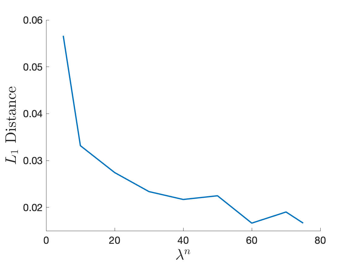
To measure the discrepancy between F(i)F^{(i)} at each iteration and the mean-field equilibrium service rate distribution in Theorem 6.9, we use the L1L_{1}-distance between these two distributions which we calculate as follows. First, we find the equilibrium solution LFL_{F} of (6.12), and calculate the mean-field equilibrium service rate μ∗​(a)\mu^{*}(a) for any trade-off parameter a~kn=a\tilde{a}_{k}^{n}=a by solving (6.9). Then, using an accurate representation for the expected idleness to be experienced as a function of μ\mu, 𝔼⁡[Ikn​(∞)|μ~kn=μ]\mathbb{E}[I_{k}^{n}(\infty)|\tilde{\mu}_{k}^{n}=\mu] given the service rate distribution F(i)F^{(i)}, we find the maximizer μi∗,n​(a)\mu_{i}^{*,n}(a) of the utility function Ukn​(μ,F(i))U_{k}^{n}(\mu,F^{(i)}) in (3.3) when a~kn=a\tilde{a}_{k}^{n}=a at iteration ii. We then calculate the desired L1L_{1}-distance as

∫aminamax|μi∗,n​(a)−μ∗​(a)|​d​Fa​(a).\int_{a_{\min}}^{a_{\max}}|\mu_{i}^{*,n}(a)-\mu^{*}(a)|dF_{a}(a).

To accurately calculate 𝔼⁡[Ikn​(∞)|μ~kn=μ]\mathbb{E}[I_{k}^{n}(\infty)|\tilde{\mu}_{k}^{n}=\mu] for any μ∈[μmin,μmax]\mu\in[\mu_{\min},\mu_{\max}] at iteration ii, we propose two approaches. The first approach uses the fluid approximation in Proposition 6.4 to approximate the expected idleness for a given service rate μ\mu replacing FF to be F(i)F^{(i)}, while the second approach estimates this quantity through extensive simulations.

Using three initial distributions, F(0)=δμmaxF^{(0)}=\delta_{\mu_{\max}}, F(0)=δμminF^{(0)}=\delta_{\mu_{\min}}, and F(0)=Uniform​(μmin,μmax)F^{(0)}=\text{Uniform}(\mu_{\min},\mu_{\max}), Figures 6.1a and 6.1b illustrate the discrepancy between the best response rates at each iteration and the mean-field equilibrium for the base-case scenario, based on the fluid and simulation approximations described above, respectively. We see that the service rate distribution converges to the equilibrium in very few iterations for all three initial distributions in both sets of experiments. In Figure 6.1c, we compare the equilibrium service rate distributions for finite-server systems, derived from the simulation approximation, with the mean-field equilibrium distribution. The figure demonstrates that the equilibrium service rate distributions converge as λn→∞\lambda^{n}\to\infty.

Figure 6.1: The convergence of best response rates to the equilibrium
Refer to caption
(a) Fluid Approximation
Refer to caption
(b) Simulation Approximation
Refer to caption
(c) Convergence as λn\lambda^{n} increases

We now examine how various functional assumptions, namely, the routing policy, cost of effort function, and utility of idleness function, affect the equilibrium mean service rate, μ¯∗\bar{\mu}^{*}, as shown in Figure 6.2c. When the random routing parameter pp approaches 0, the idleness distribution becomes more egalitarian, reducing the incentive for servers to work faster. Consequently, the equilibrium mean service rate μ¯∗\bar{\mu}^{*} decreases. Similarly, as qq increases, the marginal cost of increasing the service rate rises, leading to another decrease in μ¯∗\bar{\mu}^{*}.

In contrast, Figure 6.2c shows that the relationship between μ¯∗\bar{\mu}^{*}, NN, and rr is non-monotonic: μ¯∗\bar{\mu}^{*} initially increases with rr up to a certain point before declining. This behavior can be understood by analyzing the derivative of the utility of idleness function, uI′​(I)=r​Ir−1u_{I}^{\prime}(I)=rI^{r-1}, which first increases and then decreases as rr changes. To balance this dynamic and ensure that the marginal benefit of idleness matches the marginal cost of working harder, servers initially aim to experience more idleness as rr increases, but beyond a certain threshold, they begin to reduce the idleness they seek.

Figure 6.3b illustrates how μ¯∗\bar{\mu}^{*} and NN vary with the safety staffing level, β\beta. We observe that the equilibrium service rate μ¯∗\bar{\mu}^{*} initially increases with β\beta before decreasing. As a result, the optimal staffing level first decreases and then increases, indicating the existence of a non-trivial optimal staffing level, β\beta, that minimizes the staffing cost.

Figure 6.2: The sensitivity of the equilibrium mean service rate and the number of servers to various parameters
Refer to caption
(a) pp vs μ¯∗\bar{\mu}^{*}
Refer to caption
(b) qq vs μ¯∗\bar{\mu}^{*}
Refer to caption
(c) rr vs μ¯∗\bar{\mu}^{*}
Figure 6.3: The sensitivity of the equilibrium mean service rate and the number of servers to staffing level β\beta
Refer to caption
(a) β\beta vs μ¯∗\bar{\mu}^{*}
Refer to caption
(b) β\beta vs NN

As our final experiment, we analyze how the equilibrium distribution is affected by system parameters. Figure 6.4l illustrates the equilibrium distributions for various values of parameters as histograms. For all our distributions, we observe a sudden spike around the μ\mu with C⁡(μ,LF)=amaxC(\mu,L_{F})=a_{\max} and a decreasing density afterwards. This is a consequence of C⁡(μ,LF)C(\mu,L_{F}) having a decreasing derivative with respect to μ\mu and the distribution of a~kn\tilde{a}_{k}^{n} being uniform. To see this consider μ1<μ2\mu_{1}<\mu_{2} in the support of the service rate and take Δ>0\Delta>0. Then, we can find a1,a2,Δ1a_{1},a_{2},\Delta_{1} and Δ2\Delta_{2} such that

C(μ1,LF)=a1,C(μ1+Δ)=a1−Δ1,C(μ2)=a2 and C(μ2+Δ)=a2−Δ2.\displaystyle C(\mu_{1},L_{F})=a_{1},\qquad C(\mu_{1}+\Delta)=a_{1}-\Delta_{1},C(\mu_{2})=a_{2}\quad\mbox{ and }\quad C(\mu_{2}+\Delta)=a_{2}-\Delta_{2}.

Equation (6.9) implies ℙ⁡(μ~kn∈[μi,μi+Δ])=ℙ⁡(a~kn∈[ai−Δi],ai)\mathbb{P}(\tilde{\mu}_{k}^{n}\in[\mu_{i},\mu_{i}+\Delta])=\mathbb{P}(\tilde{a}_{k}^{n}\in[a_{i}-\Delta_{i}],a_{i}) for i=1,2i=1,2. Hence, the derivative of C⁡(μ,LF)C(\mu,L_{F}) being decreasing implies that Δ1>Δ2\Delta_{1}>\Delta_{2} and using the uniformity of a~kn\tilde{a}_{k}^{n}, we can conclude that the density of μ~kn\tilde{\mu}_{k}^{n} should be decreasing. Note that the uniformity assumption plays a key role in this conclusion and we present examples where this monotonicity property does not hold when a~kn\tilde{a}_{k}^{n} follows certain triangular distributions.

As noted above, the routing policy becomes more egalitarian as pp approaches 0, reducing the incentive for servers to work faster. Consequently, in Figure 6.4l, we observe not only a leftward shift in the distribution but also a reduction in its range indicating that the distribution spreads out more for smaller values of pp. When the cost of effort parameter qq increases, the rate of change in the cost of effort rises significantly for faster service rates compared to slower ones. This results in a leftward shift of the distribution and a less spread out distribution. For the utility of idleness parameter rr, an increase raises the value of idleness, prompting all servers to work faster and causing the distribution to shift left. Additionally, the distribution becomes more spread out, reflecting a greater impact of rr on faster servers.

Finally, the staffing parameter β\beta does not explicitly appear in (6.9), influencing the equilibrium distribution indirectly through changes in the equilibrium LFL_{F} that solves (6.12). Hence, the effect of β\beta on the distribution’s shape is relatively minor compared to other parameters. Nevertheless, as shown in Figure 6.3a, the distribution initially shifts right with increasing β\beta, indicating that when overall idleness in the system is low due to high safety staffing, servers are motivated to work faster to achieve reasonable levels of idleness. However, as β\beta becomes sufficiently large, the idleness provided by high safety staffing becomes adequate, reducing the incentive for servers to work faster.

Figure 6.4: The equilibrium distributions for different parametric setups
Refer to caption
(a) p=−1,q=2,r=0.5,β=0.4p=-1,q=2,r=0.5,\beta=0.4
Refer to caption
(b) p=−0.6,q=2,r=0.5,β=0.4p=-0.6,q=2,r=0.5,\beta=0.4
Refer to caption
(c) p=−0.2,q=2,r=0.5,β=0.4p=-0.2,q=2,r=0.5,\beta=0.4
Refer to caption
(d) p=−1,q=3,r=0.5,β=0.4p=-1,q=3,r=0.5,\beta=0.4
Refer to caption
(e) p=−1,q=4,r=0.5,β=0.4p=-1,q=4,r=0.5,\beta=0.4
Refer to caption
(f) p=−1,q=5,r=0.5,β=0.4p=-1,q=5,r=0.5,\beta=0.4
Refer to caption
(g) p=−1,q=2,r=0.25,β=0.4p=-1,q=2,r=0.25,\beta=0.4
Refer to caption
(h) p=−1,q=2,r=0.75,β=0.4p=-1,q=2,r=0.75,\beta=0.4
Refer to caption
(i) p=−1,q=2,r=1,β=0.4p=-1,q=2,r=1,\beta=0.4
Refer to caption
(j) p=−1,q=2,r=0.5,β=0.2p=-1,q=2,r=0.5,\beta=0.2
Refer to caption
(k) p=−1,q=2,r=0.5,β=0.6p=-1,q=2,r=0.5,\beta=0.6
Refer to caption
(l) p=−1,q=2,r=0.5,β=0.8p=-1,q=2,r=0.5,\beta=0.8

7 Concluding Remarks

Servers in most service systems are humans and have inherently diverse preferences and capabilities. This work introduces a framework to analyze strategic server behavior in systems with heterogeneous abilities and preferences. Specifically, it allows concave utility functions of idleness, explicitly modeling extreme discomfort from insufficient idleness, and incorporates individual preferences in balancing the utility of idleness with the cost of working faster.

Unlike prior work, where the utility of idleness is modeled linearly and a purely quality-driven regime is proven to be asymptotically optimal, we demonstrate that when discomfort grows rapidly as idleness approaches zero, the quality-and-efficiency-driven regime becomes optimal. This is the first time this conclusion appears in the literature and indicates that square-root staffing performs well even when servers act strategically.

We also provide the first detailed analysis of generalized random routing policies in a purely quality-driven regime, examining asymmetric equilibria in this context. Our results include broadly applicable sufficient conditions for the existence and uniqueness of equilibrium service rate distributions, supplemented by extensive numerical analysis of these equilibria.

This work focuses on characterizing asymptotically optimal staffing policies. Identifying optimal routing policies to improve system performance with heterogeneous strategic servers remains an open challenge. Furthermore, our analysis assumes routing policies with fairness processes that possess a density, excluding popular policies such as fastest-server-first and slowest-server-first, which require additional study. To date, research on queues with strategic servers, including this work, has largely addressed systems with a single queue and server pool. However, real-world service systems often involve multiple queues and pools, where customers and servers are categorized by needs and abilities. Investigating strategic server behavior under skill-based routing presents a particularly compelling and challenging direction for future research.

Appendices

Appendix A Proofs for Theorems

In this appendix, we present the proofs of the technical results presented in our manuscript “Many-Server Queueing Systems with Heterogeneous Strategic Servers in Heavy Traffic” and additional numerical results to justify our conclusions. The proofs are organized following the sections in the main document.

A.1 Additional Notation

In addition to the notation described in Section 1.2, we define the short-hand notation x∧y:=min⁡{x,y}x\wedge y:=\min\{x,y\}. To have a compact notation, we denote μ→:=(μ~1n,…,μ~Nαnn)\vec{\mu}:=(\tilde{\mu}_{1}^{n},\ldots,\tilde{\mu}_{N_{\alpha}^{n}}^{n}). We define dSd_{S} to be the metric for Skorokhod-J1J_{1} topology, and for any function x⁡(⋅)x(\cdot) we define |x⁡(t)|T∗:=sup0≤t≤T|x⁡(t)||x(t)|_{T}^{*}:=\sup_{0\leq t\leq T}|x(t)|. Lastly, we denote the optional quadratic variation of a stochastic process Y⁡(t)Y(t) as [Y]t[Y]_{t}.

A.2 Formal Definition of the Limiting Fairness Process

To be able to address strategic servers with heterogeneous service rates, the tool we use is the fairness process introduced by [11] and discussed in Section 3.2. The fairness process is a probability measure-valued process showing how the idleness is distributed among servers with different service rates. The name is motivated by the fact that the distribution of idleness is generally viewed as a measure of fairness towards servers see, e.g., [2, 36].

Unfortunately, it can be shown that the processes ηαπ,n\eta_{\alpha}^{\pi,n} do not converge weakly as n→∞n\to\infty in any of the four Skorokhod topologies due to the singularity around t=τ0t=\tau_{0}. Hence, to properly define the limiting fairness process, [11] suggest using shifted versions of the fairness process. For any ϵ>0\epsilon>0, the ϵ\epsilon-shifted fairness process, 𝒮ϵ​ηα,tπ,n\mathcal{S}_{\epsilon}\eta_{\alpha,t}^{\pi,n}, is defined as

𝒮ϵ​ηα,tπ,n​(𝔸):={ηα,tπ,n​(𝔸),if t>τϵn,δ0​(𝔸),if t≤τϵn,\mathcal{S}_{\epsilon}\eta_{\alpha,t}^{\pi,n}(\mathbb{A}):=\left\{\begin{array}[]{ll}\eta_{\alpha,t}^{\pi,n}(\mathbb{A})&,\mbox{if }t>\tau_{\epsilon}^{n},\\ \delta_{0}(\mathbb{A})&,\mbox{if }t\leq\tau_{\epsilon}^{n},\end{array}\right. (A.1)

for all 𝔸∈ℬ⁡(ℝ+)\mathbb{A}\in\mathcal{B}(\mathbb{R}_{+}) and ϵ>0\epsilon>0, where τϵn:=inf{t>0:∫0tI^αn​(s)​𝑑s>ϵ}\tau_{\epsilon}^{n}:=\inf\{t>0:\int_{0}^{t}\hat{I}_{\alpha}^{n}(s)ds>\epsilon\}.

The following lemma shows that the scaled idleness processes are stochastically bounded. This result is key in enabling us to study the convergence of fairness measures as well as derive fluid and diffusion limits in Section 4.

Lemma A.1.

For 1/2≤α≤11/2\leq\alpha\leq 1, the sequence of processes {(X^αn​(t))+}n∈ℕ\{(\hat{X}_{\alpha}^{n}(t))^{+}\}_{n\in\mathbb{N}}, {I^αn​(t)}n∈ℕ\{\hat{I}_{\alpha}^{n}(t)\}_{n\in\mathbb{N}} are stochastically bounded.

Proof.

Lemma 1 in [11] provides the proof for α=1/2\alpha=1/2, and hence, we concentrate on the cases where 1/2<α≤11/2<\alpha\leq 1. Let T>0T>0, n∈ℕn\in\mathbb{N}, and set θn,0:=inf{t≥0:(X^αn​(t))+=0}\theta^{n,0}:=\inf\{t\geq 0:(\hat{X}_{\alpha}^{n}(t))^{+}=0\}. Then, we have

ℙ⁡(|(X^αn​(t))+|T∗>M)\displaystyle\mathbb{P}\left(\left|(\hat{X}_{\alpha}^{n}(t))^{+}\right|_{T}^{*}>M\right) ≤ℙ(|(X^αn(t))+|T∧θn,0∗>M)+ℙ(supθn,0≤t≤T|(X^αn(t))+|>M,θn,0<T).\displaystyle\leq\mathbb{P}\left(\left|(\hat{X}_{\alpha}^{n}(t))^{+}\right|_{T\wedge\theta^{n,0}}^{*}>M\right)+\mathbb{P}\left(\sup_{\theta^{n,0}\leq t\leq T}\left|(\hat{X}_{\alpha}^{n}(t))^{+}\right|>M,\theta^{n,0}<T\right).

For all 0≤t≤T∧θn,00\leq t\leq T\wedge\theta^{n,0},

(X^αn​(t))+\displaystyle(\hat{X}_{\alpha}^{n}(t))^{+} ≤(X^αn​(0))++n−α​An​(t)−n−α​∑k=1NαnSk​(μ~kn​t),\displaystyle\leq(\hat{X}_{\alpha}^{n}(0))^{+}+n^{-\alpha}A^{n}(t)-n^{-\alpha}\sum_{k=1}^{N_{\alpha}^{n}}S_{k}(\tilde{\mu}_{k}^{n}t),
≤(X^αn​(0))++n−α​(An​(t)−λn​t)−n−α​∑k=1Nαn(Sk​(μ~kn​t)−μ~kn​t)\displaystyle\leq(\hat{X}_{\alpha}^{n}(0))^{+}+n^{-\alpha}\left(A^{n}(t)-\lambda^{n}t\right)-n^{-\alpha}\sum_{k=1}^{N_{\alpha}^{n}}\left(S_{k}(\tilde{\mu}_{k}^{n}t)-\tilde{\mu}_{k}^{n}t\right)
+n−α​(λn−Nαn​μ¯F)​t−n−α​∑k=1Nαn(μ~kn−μ¯F)​t\displaystyle\quad+n^{-\alpha}\left(\lambda^{n}-N_{\alpha}^{n}\bar{\mu}_{F}\right)t-n^{-\alpha}\sum_{k=1}^{N_{\alpha}^{n}}\left(\tilde{\mu}_{k}^{n}-\bar{\mu}_{F}\right)t
→pξ0−β​λ¯α​μ¯F1−α​t,\displaystyle\stackrel{{\scriptstyle p}}{{\rightarrow}}\xi_{0}-\beta\bar{\lambda}^{\alpha}\bar{\mu}_{F}^{1-\alpha}t, (A.2)

where we use the martingale central limit theorem c.f. [32] to prove convergence of the centered Poisson processes along with Assumption 3.2, the definition of NαnN_{\alpha}^{n} in (3.1) and the central limit theorem. Defining θϵn,1:=inf{s>θn,0:(X^αn​(s))+>ϵ}\theta_{\epsilon}^{n,1}:=\inf\big\{s>\theta^{n,0}:\big(\hat{X}_{\alpha}^{n}(s)\big)^{+}>\epsilon\big\} and θ~ϵn,1:=sup{θn,0≤s<θϵn,1:(X^αn​(s))+<ϵ/2}\tilde{\theta}_{\epsilon}^{n,1}:=\sup\big\{\theta^{n,0}\leq s<\theta_{\epsilon}^{n,1}:\big(\hat{X}_{\alpha}^{n}(s)\big)^{+}<\epsilon/2\big\},

ℙ⁡(supθn,0≤s≤T(X^αn​(s))+>ϵ)\displaystyle\mathbb{P}\left(\sup_{\theta^{n,0}\leq s\leq T}\big(\hat{X}_{\alpha}^{n}(s)\big)^{+}>\epsilon\right) ≤ℙ⁡(θn,0<θ~ϵn,1≤θϵn,1≤T)\displaystyle\leq\mathbb{P}\left(\theta^{n,0}<\tilde{\theta}_{\epsilon}^{n,1}\leq\theta_{\epsilon}^{n,1}\leq T\right)
≤ℙ(supθn,0≤s1<s2≤T{|An​(s2)−An​(s1)−λn​(s2−s1)nα|\displaystyle\leq\mathbb{P}\left(\sup_{\theta^{n,0}\leq s_{1}<s_{2}\leq T}\left\{\left|\frac{A^{n}(s_{2})-A^{n}(s_{1})-\lambda^{n}(s_{2}-s_{1})}{n^{\alpha}}\right|\right.\right.
+|∑k=1Nαn(Sk​(μ~k​s2)−Sk​(μ~k​s1)−μ~k​(s2−s1))nα|\displaystyle\qquad\qquad\qquad+\left.\left|\frac{\sum_{k=1}^{N^{n}_{\alpha}}\big(S_{k}(\tilde{\mu}_{k}s_{2})-S_{k}(\tilde{\mu}_{k}s_{1})-\tilde{\mu}_{k}(s_{2}-s_{1})\big)}{n^{\alpha}}\right|\right.
+|(λn−∑k=1Nαnμ~k)​(s2−s1)nα|}>ϵ/2)\displaystyle\qquad\qquad\qquad\qquad\qquad\qquad\quad\left.\left.+\left|\frac{(\lambda^{n}-\sum_{k=1}^{N_{\alpha}^{n}}\tilde{\mu}_{k})(s_{2}-s_{1})}{n^{\alpha}}\right|\right\}>\epsilon/2\right)
≤2​ℙ​(n−α​|An​(s)−λn​s|T∗>ϵ/16)\displaystyle\leq 2\mathbb{P}\left(n^{-\alpha}|A^{n}(s)-\lambda^{n}s|_{T}^{*}>\epsilon/16\right)
+2​ℙ​(n−α​|∑k=1NαnSkn​(s)−μ~kn​s|T∗>ϵ/16)\displaystyle\qquad+2\mathbb{P}\left(n^{-\alpha}\left|\sum_{k=1}^{N_{\alpha}^{n}}S_{k}^{n}(s)-\tilde{\mu}_{k}^{n}s\right|_{T}^{*}>\epsilon/16\right)
+ℙ⁡(n−α​(λn−∑k=1Nαnμ~k)>0).\displaystyle\qquad+\mathbb{P}\left(n^{-\alpha}\left(\lambda^{n}-\sum_{k=1}^{N_{\alpha}^{n}}\tilde{\mu}_{k}\right)>0\right). (A.3)

Again, using the martingale central limit theorem and the central limit theorem, the right-hand side of (A.3) converges to 00, and combining (A.2) and (A.3) we obtain the stochastic boundedness of {(X^αn​(t))+}n∈ℕ\{(\hat{X}_{\alpha}^{n}(t))^{+}\}_{n\in\mathbb{N}}.

We now prove the stochastic boundedness of {I^αn​(t)}n∈ℕ\{\hat{I}_{\alpha}^{n}(t)\}_{n\in\mathbb{N}}. We have

|I^αn​(t)|T∗\displaystyle\left|\hat{I}_{\alpha}^{n}(t)\right|_{T}^{*} ≤|X^αn​(0)|+|An​(t)−λn​tnα|T∗+|∑k=1NαnSkn​(t)−μkn​tnα|T∗+|∑k=1Nαnμkn​t−λn​tnα|T∗\displaystyle\leq\left|\hat{X}_{\alpha}^{n}(0)\right|+\left|\frac{A^{n}(t)-\lambda^{n}t}{n^{\alpha}}\right|_{T}^{*}+\left|\frac{\sum_{k=1}^{N_{\alpha}^{n}}S_{k}^{n}(t)-\mu_{k}^{n}t}{n^{\alpha}}\right|_{T}^{*}+\left|\frac{\sum_{k=1}^{N_{\alpha}^{n}}\mu_{k}^{n}t-\lambda^{n}t}{n^{\alpha}}\right|_{T}^{*}
+|Rn​(γ​∫0t(Xn​(s)−Nαn)+​𝑑s)−γ​∫0t(Xn​(s)−Nαn)+​𝑑snα|T∗+|γ​∫0t(X^αn​(s))+​𝑑s|T∗.\displaystyle\quad+\left|\frac{R^{n}\left(\gamma\int_{0}^{t}(X^{n}(s)-N_{\alpha}^{n})^{+}ds\right)-\gamma\int_{0}^{t}(X^{n}(s)-N_{\alpha}^{n})^{+}ds}{n^{\alpha}}\right|_{T}^{*}+\left|\gamma\int_{0}^{t}(\hat{X}_{\alpha}^{n}(s))^{+}ds\right|_{T}^{*}.

The stochastic boundedness of {(X^αn​(t))+}n∈ℕ\{(\hat{X}_{\alpha}^{n}(t))^{+}\}_{n\in\mathbb{N}} and the martingale central limit theorem implies the stochastic boundedness of the last two terms. The second and third terms are stochastically bounded again due to the martingale central limit theorem. Finally, the first and the fourth terms are stochastically bounded due to Assumption 3.2 and the central limit theorem. This proves the lemma. ∎

Using Lemma A.1, it is straightforward to prove the tightness of the continuous processes {∫0tI^αn​(s)​𝑑s}n∈ℕ\left\{\int_{0}^{t}\hat{I}_{\alpha}^{n}(s)ds\right\}_{n\in\mathbb{N}} and that {τϵn∧T}n∈ℕ\{\tau_{\epsilon}^{n}\wedge T\}_{n\in\mathbb{N}} are continuous functionals of these processes.

Definition A.2.

Suppose τϵn∧T⇒τϵ∧T\tau_{\epsilon}^{n}\wedge T\Rightarrow\tau_{\epsilon}\wedge T for all ϵ,T>0\epsilon,T>0 as n→∞n\to\infty. A process {ηα,tπ}t≥0\{\eta_{\alpha,t}^{\pi}\}_{t\geq 0} is called the limiting fairness process if for all ϵ>0\epsilon>0, it holds that 𝒮ϵ​ηαπ,n⇒𝒮ϵ​ηαπ\mathcal{S}_{\epsilon}\eta_{\alpha}^{\pi,n}\Rightarrow\mathcal{S}_{\epsilon}\eta_{\alpha}^{\pi} as n→∞n\to\infty in the Skorokhod-J1J_{1} topology modified for left-continuous functions, and where 𝒮ϵ​ηαπ\mathcal{S}_{\epsilon}\eta_{\alpha}^{\pi} is defined by replacing ηα,tπ,n\eta_{\alpha,t}^{\pi,n} and τϵn\tau_{\epsilon}^{n} in (A.1) by ηα,tπ\eta_{\alpha,t}^{\pi} and τϵ\tau_{\epsilon}.

The following result generalizes Theorem 2 in [11] from α=1/2\alpha=1/2 to 1/2≤α≤11/2\leq\alpha\leq 1, and is a step towards establishing the existence of a limiting fairness process. The proof is a direct adaptation of that in [11] and is omitted here.

Proposition A.3.

For ϵ>0\epsilon>0 and 1/2≤α≤11/2\leq\alpha\leq 1, the shifted fairness processes {𝒮ϵ​ηαπ,n}n∈ℤ+\{\mathcal{S}_{\epsilon}\eta_{\alpha}^{\pi,n}\}_{n\in\mathbb{Z}_{+}} are tight under any non-idling policy.

A.3 Proofs for Results Presented in Section 4

Proof of Theorem 4.1.

Our proof follows the same steps as Theorem 5 in [11] with the additional modification on the number of servers. To simplify the notation, we suppress the π\pi superscript of the fairness process. Adding and subtracting appropriate terms to (3.7) and normalizing with nαn^{\alpha}, we get

X^αn​(t)\displaystyle\hat{X}_{\alpha}^{n}(t) =X^αn​(0)+M^α,1n​(t)−M^α,2n​(t)−M^α,3n​(t)+n−α​(λn−Nαn​μ¯F)​t−n−α​(∑k=1Nαnμ~kn−Nαn​μ¯F)​t\displaystyle=\hat{X}_{\alpha}^{n}(0)+\hat{M}_{\alpha,1}^{n}(t)-\hat{M}_{\alpha,2}^{n}(t)-\hat{M}_{\alpha,3}^{n}(t)+n^{-\alpha}(\lambda^{n}-N_{\alpha}^{n}\bar{\mu}_{F})t-n^{-\alpha}\left(\sum_{k=1}^{N_{\alpha}^{n}}\tilde{\mu}_{k}^{n}-N_{\alpha}^{n}\bar{\mu}_{F}\right)t
−∑k=1Nαnμ~kn∫0tI^k,αn(s)ds−γ∫0t(X^αn(s))+ds,\displaystyle\quad-\sum_{k=1}^{N_{\alpha}^{n}}\tilde{\mu}_{k}^{n}\int_{0}^{t}\hat{I}_{k,\alpha}^{n}(s)ds-\gamma\int_{0}^{t}(\hat{X}_{\alpha}^{n}(s))^{+}ds, (A.4)

where

M^α,1n​(t)\displaystyle\displaystyle\hat{M}_{\alpha,1}^{n}(t) :=An​(t)−λn​tnα,\displaystyle:=\frac{A^{n}(t)-\lambda^{n}t}{n^{\alpha}},
M^α,2n​(t)\displaystyle\hat{M}_{\alpha,2}^{n}(t) :=Sn​(∑k=1Nαnμ~kn​(t−∫0tIkn​(s)​𝑑s))−∑k=1Nαnμ~kn​(t−∫0tIkn​(s)​𝑑s)nα,\displaystyle:=\frac{S^{n}\left(\sum_{k=1}^{N_{\alpha}^{n}}\tilde{\mu}_{k}^{n}\left(t-\int_{0}^{t}I_{k}^{n}(s)ds\right)\right)-\sum_{k=1}^{N_{\alpha}^{n}}\tilde{\mu}_{k}^{n}\left(t-\int_{0}^{t}I_{k}^{n}(s)ds\right)}{n^{\alpha}},
M^α,3n​(t)\displaystyle\displaystyle\hat{M}_{\alpha,3}^{n}(t) :=Rn​(γ​∫0t(Xn​(s)−Nαn)+​𝑑s)−γ​∫0t(Xn​(s)−Nαn)+​𝑑snα.\displaystyle:=\frac{R^{n}\left(\gamma\int_{0}^{t}(X^{n}(s)-N_{\alpha}^{n})^{+}ds\right)-\gamma\int_{0}^{t}(X^{n}(s)-N_{\alpha}^{n})^{+}ds}{n^{\alpha}}.

Using the martingale central limit theorem, both M^α,1n​(t)\hat{M}_{\alpha,1}^{n}(t) and M^α,2n​(t)\hat{M}_{\alpha,2}^{n}(t) converge weakly to 00 when α>1/2\alpha>1/2 and to λ¯​W​(t)\sqrt{\bar{\lambda}}W(t), where W⁡(t)W(t) is a standard Brownian motion when α=1/2\alpha=1/2. To see this, we focus on M^α,2n\hat{M}_{\alpha,2}^{n}. The process Mα,2n​(t)M_{\alpha,2}^{n}(t) is a compensated Poisson process and is a martingale with predictable quadratic variation

∑k=1Nαnμ~kn​(t−∫0tIkn​(s)​𝑑s)n2​α=Nαnn2​α​∑k=1Nαnμ~kn​tNαn−∑k=1Nαnμ~kn​∫0tIkn​(s)​𝑑sn2​α.\frac{\sum_{k=1}^{N_{\alpha}^{n}}\tilde{\mu}_{k}^{n}\left(t-\int_{0}^{t}I_{k}^{n}(s)ds\right)}{n^{2\alpha}}=\frac{N_{\alpha}^{n}}{n^{2\alpha}}\frac{\sum_{k=1}^{N_{\alpha}^{n}}\tilde{\mu}_{k}^{n}t}{N_{\alpha}^{n}}-\frac{\sum_{k=1}^{N_{\alpha}^{n}}\tilde{\mu}_{k}^{n}\int_{0}^{t}I_{k}^{n}(s)ds}{n^{2\alpha}}.

The stochastic boundedness of {I^αn}n∈ℕ\{\hat{I}_{\alpha}^{n}\}_{n\in\mathbb{N}} (Lemma A.1) and the boundedness of μ~kn\tilde{\mu}_{k}^{n} imply that the second term on the right-hand side converges to 00 for all 1/2≤α≤11/2\leq\alpha\leq 1. Using the law of large numbers, the first term converges to 00 if α>1/2\alpha>1/2 and to λ¯\bar{\lambda} if α=1/2\alpha=1/2. The jumps of Mα,2n​(t)M_{\alpha,2}^{n}(t) are bounded by 1/nα1/n^{\alpha}, hence the martingale central limit theorem implies that M^1/2,2n​(t)⇒λ¯​W​(t)\hat{M}_{1/2,2}^{n}(t)\Rightarrow\sqrt{\bar{\lambda}}W(t) and M^α,2n​(t)→p0\hat{M}_{\alpha,2}^{n}(t)\stackrel{{\scriptstyle p}}{{\rightarrow}}0 when α>1/2\alpha>1/2. The proof for M^α,1n​(t)\hat{M}_{\alpha,1}^{n}(t) follows the same steps. Similarly, M^α,3n​(t)⇒0\hat{M}_{\alpha,3}^{n}(t)\Rightarrow 0 for all α≥1/2\alpha\geq 1/2 as a result of the stochastic boundedness of {(X^αn)+}n∈ℕ\{(\hat{X}_{\alpha}^{n})^{+}\}_{n\in\mathbb{N}} in Lemma A.1. Plugging in (3.1), we get n−α​(λn−Nαn​μ¯F)​t→−β​λ¯α​μ¯F1−α​tn^{-\alpha}(\lambda^{n}-N_{\alpha}^{n}\bar{\mu}_{F})t\to-\beta\bar{\lambda}^{\alpha}\bar{\mu}_{F}^{1-\alpha}t. Finally, using the central limit theorem, we have n−α​(∑k=1Nαnμ~kn−Nαn​μ¯F)​t→p0n^{-\alpha}\left(\sum_{k=1}^{N_{\alpha}^{n}}\tilde{\mu}_{k}^{n}-N_{\alpha}^{n}\bar{\mu}_{F}\right)t\stackrel{{\scriptstyle p}}{{\rightarrow}}0 for α>1/2\alpha>1/2 and n−α​(∑k=1Nαnμ~kn−Nαn​μ¯F)​t⇒ζ​λ¯α​μ¯F−α​tn^{-\alpha}\left(\sum_{k=1}^{N_{\alpha}^{n}}\tilde{\mu}_{k}^{n}-N_{\alpha}^{n}\bar{\mu}_{F}\right)t\Rightarrow\zeta\bar{\lambda}^{\alpha}\bar{\mu}_{F}^{-\alpha}t for α=1/2\alpha=1/2, where ζ\zeta is a normal random variable with mean 0 and variance σF2\sigma_{F}^{2}. As 𝒮ϵ​ηα,tn⇒𝒮ϵ​ηα,t\mathcal{S}_{\epsilon}\eta_{\alpha,t}^{n}\Rightarrow\mathcal{S}_{\epsilon}\eta_{\alpha,t} for any ϵ>0\epsilon>0, using Lemma 2 in [11], a modification of the Skorokhod representation theorem, we can assume that all the above processes converge w.p. 1 and to prove the theorem, we need only to prove that for any ρ>0\rho>0, ℙ⁡(dS​(X^αn,ξα)>ρ)→0\mathbb{P}(d_{S}(\hat{X}_{\alpha}^{n},\xi_{\alpha})>\rho)\to 0 as n→∞n\to\infty.

For any ϖ>0\varpi>0, we can find a sequence of homeomorphisms Λn​(t):[0,T]→[0,T]\Lambda^{n}(t):[0,T]\to[0,T] with derivative Λ˙n​(t)\dot{\Lambda}^{n}(t) and NϖN_{\varpi} such that for any n>Nϖn>N_{\varpi},

|M^α,1n​(t)+M^α,2n​(t)+M^α,3n​(t)−2​λ​W​(Λn​(t))|T∗∨|⟨ι,𝒮ϵ​ηα,tn⟩−⟨ι,𝒮ϵ​ηα,Λn​(t)⟩|T∗∨|Λ˙n​(t)−1|T∗<ϖ,\left|\hat{M}_{\alpha,1}^{n}(t)+\hat{M}_{\alpha,2}^{n}(t)+\hat{M}_{\alpha,3}^{n}(t)-\sqrt{2\lambda}W(\Lambda^{n}(t))\right|_{T}^{*}\vee\left|\langle\iota,\mathcal{S}_{\epsilon}\eta_{\alpha,t}^{n}\rangle-\langle\iota,\mathcal{S}_{\epsilon}\eta_{\alpha,\Lambda^{n}(t)}\rangle\right|_{T}^{*}\vee\left|\dot{\Lambda}^{n}(t)-1\right|_{T}^{*}<\varpi,

if α=1/2\alpha=1/2 and

|M^α,1n​(t)+M^α,2n​(t)+M^α,3n​(t)|T∗∨|⟨ι,𝒮ϵ​ηα,tn⟩−⟨ι,𝒮ϵ​ηα,Λn​(t)⟩|T∗∨|Λ˙n​(t)−1|T∗<ϖ,\left|\hat{M}_{\alpha,1}^{n}(t)+\hat{M}_{\alpha,2}^{n}(t)+\hat{M}_{\alpha,3}^{n}(t)\right|_{T}^{*}\vee\left|\langle\iota,\mathcal{S}_{\epsilon}\eta_{\alpha,t}^{n}\rangle-\langle\iota,\mathcal{S}_{\epsilon}\eta_{\alpha,\Lambda^{n}(t)}\rangle\right|_{T}^{*}\vee\left|\dot{\Lambda}^{n}(t)-1\right|_{T}^{*}<\varpi,

if 1/2<α≤11/2<\alpha\leq 1. We will prove our result by showing

sup0≤t≤T|X^αn​(t)−ξα​(Λn​(t))|→0,w.p. ​1.\sup_{0\leq t\leq T}\left|\hat{X}_{\alpha}^{n}(t)-\xi_{\alpha}(\Lambda^{n}(t))\right|\to 0,\mbox{w.p. }1. (A.5)

Using the tightness of the processes, without loss of generality, we can assume that

supn∈ℕ{|⟨ι,ηα,tn⟩|T∗∨|X^αn​(t)|T∗∨|ξα​(t)|T∗}<K.\sup_{n\in\mathbb{N}}\left\{\left|\langle\iota,\eta_{\alpha,t}^{n}\rangle\right|_{T}^{*}\vee\left|\hat{X}_{\alpha}^{n}(t)\right|_{T}^{*}\vee\left|\xi_{\alpha}(t)\right|_{T}^{*}\right\}<K.

Now, taking ξα​(t)\xi_{\alpha}(t) to be the solution of the appropriate equation in the statement of the theorem, plugging in the definition of fairness process for the seventh term on the right-hand side of (A.4), for any ϖ\varpi we have an NϖN_{\varpi} such that n>Nϖn>N_{\varpi} implies

|X^αn​(t)−ξ⁡(Λn​(t))|\displaystyle|\hat{X}_{\alpha}^{n}(t)-\xi(\Lambda^{n}(t))| ≤ϖ+γ​|∫0t(X^αn​(s))+​𝑑s−∫0Λn​(t)(ξ⁡(s))+​𝑑s|\displaystyle\leq\varpi+\gamma\left|\int_{0}^{t}(\hat{X}_{\alpha}^{n}(s))^{+}ds-\int_{0}^{\Lambda^{n}(t)}(\xi(s))^{+}ds\right|
+|⟨ι,ηα,tn⟩​∫0t(X^αn​(s))−​𝑑s−⟨ι,ηα,Λn​(t)⟩​∫0Λn​(t)(ξ⁡(s))−​𝑑s|.\displaystyle\qquad+\left|\langle\iota,\eta_{\alpha,t}^{n}\rangle\int_{0}^{t}(\hat{X}_{\alpha}^{n}(s))^{-}ds-\langle\iota,\eta_{\alpha,\Lambda^{n}(t)}\rangle\int_{0}^{\Lambda^{n}(t)}(\xi(s))^{-}ds\right|. (A.6)

We can bound the second term on the right-hand side of (A.6) as

|∫0t(X^αn​(s))+​𝑑s−∫0Λn​(t)(ξ⁡(s))+​𝑑s|\displaystyle\left|\int_{0}^{t}(\hat{X}_{\alpha}^{n}(s))^{+}ds-\int_{0}^{\Lambda^{n}(t)}(\xi(s))^{+}ds\right| ≤∫0t|X^αn​(s)−ξα​(Λn​(s))​𝑑s|+∫0t|(1−Λ˙n​(t))​ξα​(Λn​(s))|​𝑑s\displaystyle\leq\int_{0}^{t}\left|\hat{X}_{\alpha}^{n}(s)-\xi_{\alpha}(\Lambda^{n}(s))ds\right|+\int_{0}^{t}\left|(1-\dot{\Lambda}^{n}(t))\xi_{\alpha}(\Lambda^{n}(s))\right|ds
≤∫0t|X^αn​(s)−ξα​(Λn​(s))​𝑑s|+ϖ​K​t.\displaystyle\leq\int_{0}^{t}\left|\hat{X}_{\alpha}^{n}(s)-\xi_{\alpha}(\Lambda^{n}(s))ds\right|+\varpi Kt.

To bound the third term on the right-hand side of (A.6),

|⟨ι,ηα,tn⟩​∫0t(X^αn​(s))−​𝑑s−⟨ι,ηα,Λn​(t)⟩​∫0Λ⁡(t)(ξ⁡(s))−​𝑑s|\displaystyle\left|\langle\iota,\eta^{n}_{\alpha,t}\rangle\int_{0}^{t}(\hat{X}_{\alpha}^{n}(s))^{-}ds-\langle\iota,\eta_{\alpha,\Lambda^{n}(t)}\rangle\int_{0}^{\Lambda(t)}(\xi(s))^{-}ds\right|
≤|(⟨ι,ηα,tn⟩−⟨ι,𝒮ϵ​ηα,tn⟩)​∫0t(X^αn​(s))−​𝑑s−(⟨ι,ηα,Λn​(t)⟩−⟨ι,𝒮ϵ​ηα,Λn​(t)⟩)​∫0Λ⁡(t)(ξα​(s))−​𝑑s|\displaystyle\leq\left|\left(\langle\iota,\eta_{\alpha,t}^{n}\rangle-\langle\iota,\mathcal{S}_{\epsilon}\eta_{\alpha,t}^{n}\rangle\right)\int_{0}^{t}(\hat{X}_{\alpha}^{n}(s))^{-}ds-\left(\langle\iota,\eta_{\alpha,\Lambda^{n}(t)}\rangle-\langle\iota,\mathcal{S}_{\epsilon}\eta_{\alpha,\Lambda^{n}(t)}\rangle\right)\int_{0}^{\Lambda(t)}(\xi_{\alpha}(s))^{-}ds\right|
+|(⟨ι,𝒮ϵ​ηα,tn⟩−⟨ι,𝒮ϵ​ηα,Λn​(t)⟩)​∫0t(X^αn​(s))−​𝑑s−⟨ι,𝒮ϵ​ηα,Λn​(t)⟩​∫0t((X^αn​(s))−−(ξα​(Λ⁡(s)))−)​𝑑s|\displaystyle\;+\left|\left(\langle\iota,\mathcal{S}_{\epsilon}\eta_{\alpha,t}^{n}\rangle-\langle\iota,\mathcal{S}_{\epsilon}\eta_{\alpha,\Lambda^{n}(t)}\rangle\right)\int_{0}^{t}(\hat{X}_{\alpha}^{n}(s))^{-}ds-\langle\iota,\mathcal{S}_{\epsilon}\eta_{\alpha,\Lambda^{n}(t)}\rangle\int_{0}^{t}\left(\Big(\hat{X}_{\alpha}^{n}(s)\Big)^{-}-\Big(\xi_{\alpha}(\Lambda(s))\Big)^{-}\right)ds\right|
+|⟨ι,𝒮ϵ​ηα,Λn​(t)⟩​∫0t(1−Λ˙​(s))​(ξα​(Λ⁡(s)))−​𝑑s|\displaystyle\;+\left|\langle\iota,\mathcal{S}_{\epsilon}\eta_{\alpha,\Lambda^{n}(t)}\rangle\int_{0}^{t}(1-\dot{\Lambda}(s))\big(\xi_{\alpha}(\Lambda(s))\big)^{-}ds\right|
≤(2​ϵ+ϖ⁡(1+K))​K​t+K​∫0t|X^n​(s)−ξ^​(Λ⁡(s))|​𝑑s.\displaystyle\leq(2\epsilon+\varpi(1+K))Kt+K\int_{0}^{t}\left|\hat{X}^{n}(s)-\hat{\xi}(\Lambda(s))\right|ds.

Plugging these bounds in (A.6), using Grönwall’s inequality, and choosing ϵ\epsilon and ϖ\varpi appropriately, our result follows. ∎

Now, we prove the interchangeability of many-server limit and limit as t→∞t\to\infty. To do so, we need the following uniform integrability result.

Lemma A.4.

For any 1/2≤α≤11/2\leq\alpha\leq 1, the stationary scaled system lengths {X^n​(∞)}n∈ℕ\{\hat{X}^{n}(\infty)\}_{n\in\mathbb{N}} are uniformly integrable and hence tight.

Proof.

For any n∈ℕn\in\mathbb{N}, we decompose the scaled system length process into its negative and positive parts as

X^αn​(∞)=(X^αn​(∞))+−(X^αn​(∞))−,\hat{X}_{\alpha}^{n}(\infty)=\left(\hat{X}_{\alpha}^{n}(\infty)\right)^{+}-\left(\hat{X}_{\alpha}^{n}(\infty)\right)^{-},

and prove the uniform integrability of each part separately. We consider (X^αn​(t))−\left(\hat{X}_{\alpha}^{n}(t)\right)^{-} and use a coupling argument. Now, suppose we fix n>0n>0 and let θA,in\theta_{A,i}^{n} be the occurrence time of the iith event for Poisson process An​(t)A^{n}(t). Assume that we know (μ~1n,…,μ~Nαnn)(\tilde{\mu}_{1}^{n},\ldots,\tilde{\mu}_{N_{\alpha}^{n}}^{n}) and define S~n​(t)\tilde{S}^{n}(t) to be a Poisson process with rate ∑k=1Nαnμ~kn\sum_{k=1}^{N^{n}_{\alpha}}\tilde{\mu}_{k}^{n} and let θS,in\theta_{S,i}^{n} be the occurrence time for the iith event. We also define a sequence {Uin}i∈ℕ\{U_{i}^{n}\}_{i\in\mathbb{N}} of independent uniform(0,1) random variables. For any given time tt, we know that the system should be serving with a rate equal to the sum of service rates of busy servers, i.e., ∑k=1Nαnμ~kn​(1−Ikn​(t))\sum_{k=1}^{N^{n}_{\alpha}}\tilde{\mu}_{k}^{n}(1-I_{k}^{n}(t)), hence we use the thinning property of Poisson process where event ii of S~n​(t)\tilde{S}^{n}(t) is accepted as an actual departure with probability pin​(θSin−)=∑k=1Nαnμ~kn​(1−Ikn​(θS,in−))∑k=1Nαnμ~knp_{i}^{n}(\theta_{S_{i}}^{n}-)=\frac{\sum_{k=1}^{N^{n}_{\alpha}}\tilde{\mu}_{k}^{n}(1-I_{k}^{n}(\theta_{S,i}^{n}-))}{\sum_{k=1}^{N^{n}_{\alpha}}\tilde{\mu}_{k}^{n}} by checking whether Uin≤pin​(θSin−)U_{i}^{n}\leq p_{i}^{n}(\theta_{S_{i}}^{n}-) or not. The processes Ikn​(t)I_{k}^{n}(t) can be rigorously defined by using UinU_{i}^{n}s and a routing process based on our routing policy. As this does not play a major role in our proof, we refer the reader to [11] for the detailed construction of idleness processes. Now, we can write

(X^αn​(t))−=(X^αn​(0))−\displaystyle\left(\hat{X}_{\alpha}^{n}(t)\right)^{-}=\left(\hat{X}_{\alpha}^{n}(0)\right)^{-} +n−α∑i=1S~n​(t)𝕀((X^αn(θS,in−))+=0)𝕀(Uin≤pin(θSin−))\displaystyle+n^{-\alpha}\sum_{i=1}^{\tilde{S}^{n}(t)}\mathbb{I}\left(\left(\hat{X}_{\alpha}^{n}(\theta_{S,i}^{n}-)\right)^{+}=0\right)\mathbb{I}\Big(U_{i}^{n}\leq p_{i}^{n}\left(\theta_{S_{i}}^{n}-\right)\Big)
−n−α∑i=1An​(t)𝕀((X^αn(θA,in−))−>0).\displaystyle-n^{-\alpha}\sum_{i=1}^{A^{n}(t)}\mathbb{I}\left(\left(\hat{X}_{\alpha}^{n}(\theta_{A,i}^{n}-)\right)^{-}>0\right).

We define a birth-death process {Y1n​(t)}n∈ℕ\{Y_{1}^{n}(t)\}_{n\in\mathbb{N}} with Y1n​(0)=(Xn​(0))−Y_{1}^{n}(0)=\left(X^{n}(0)\right)^{-} w.p.1, whose birth rate at Yn​(t)=iY^{n}(t)=i is ∑k=1μ~kn−μmin​i\sum_{k=1}\tilde{\mu}_{k}^{n}-\mu_{\min}i and death rate is λn\lambda^{n} if Y1n​(t)>0Y_{1}^{n}(t)>0. Then, we can couple the scaled process Y^1n​(t)=n−α​Y1n​(t)\hat{Y}_{1}^{n}(t)=n^{-\alpha}Y_{1}^{n}(t) with the system length process by writing it as

Y^1n​(t)\displaystyle\hat{Y}_{1}^{n}(t) =Y^1n​(0)+n−α​∑i=1S~n​(t)𝕀⁡(Uin≤p~in​(θS,in−))−n−α​∑i=1An​(t)𝕀⁡(Y^1n​(θA,in−)>0),\displaystyle=\hat{Y}_{1}^{n}(0)+n^{-\alpha}\sum_{i=1}^{\tilde{S}^{n}(t)}\mathbb{I}\Big(U_{i}^{n}\leq\tilde{p}_{i}^{n}\left(\theta_{S,i}^{n}-\right)\Big)-n^{-\alpha}\sum_{i=1}^{A^{n}(t)}\mathbb{I}\left(\hat{Y}_{1}^{n}(\theta_{A,i}^{n}-)>0\right),

where p~in​(θSin−):=∑k=1Nαnμ~kn−μmin​Y^1​(θSin−)∑k=1Nnμ~kn\tilde{p}_{i}^{n}\left(\theta_{S_{i}}^{n}-\right):=\frac{\sum_{k=1}^{N^{n}_{\alpha}}\tilde{\mu}_{k}^{n}-\mu_{\min}\hat{Y}_{1}\left(\theta_{S_{i}}^{n}-\right)}{\sum_{k=1}^{N^{n}}\tilde{\mu}_{k}^{n}}. To see that (X^αn​(t))−≤Y^1n​(t)\left(\hat{X}_{\alpha}^{n}(t)\right)^{-}\leq\hat{Y}_{1}^{n}(t) for all t≥0t\geq 0 with probability 1, define ϑn={t:(X^αn​(t))−>Y^1n​(t)}\vartheta^{n}=\left\{t:\left(\hat{X}_{\alpha}^{n}(t)\right)^{-}>\hat{Y}_{1}^{n}(t)\right\}. As at most one event occurs at any given time tt with probability 1, we have (X^αn​(ϑn−))−=Y^1n​(ϑn−)\left(\hat{X}_{\alpha}^{n}(\vartheta^{n}-)\right)^{-}=\hat{Y}_{1}^{n}(\vartheta^{n}-). By definition we have

p~in​(ϑn−)≥pin​(ϑn−).\tilde{p}_{i}^{n}\left(\vartheta^{n}-\right)\geq p_{i}^{n}(\vartheta^{n}-).

Hence, if ϑn\vartheta^{n} is an event epoch for S~n​(t)\tilde{S}^{n}(t), we have (X^αn​(ϑn))−≤Y^1n​(ϑn)\left(\hat{X}_{\alpha}^{n}(\vartheta^{n})\right)^{-}\leq\hat{Y}_{1}^{n}(\vartheta^{n}) and if ϑn\vartheta^{n} is an event epoch for An​(t)A^{n}(t), we have (X^αn​(ϑn))−=Y^1n​(ϑn)\left(\hat{X}_{\alpha}^{n}(\vartheta^{n})\right)^{-}=\hat{Y}_{1}^{n}(\vartheta^{n}), both contradicts with the definition of ϑn\vartheta^{n}. Hence, we conclude that (X^αn​(t))−≤Y^1n​(t)\left(\hat{X}_{\alpha}^{n}(t)\right)^{-}\leq\hat{Y}_{1}^{n}(t) for all t≥0t\geq 0 with probability 1.

Now, define ζn:=n−α​(∑k=1Nαnμ~kn−Nαn​μ¯)\zeta^{n}:=n^{-\alpha}\left(\sum_{k=1}^{N^{n}_{\alpha}}\tilde{\mu}_{k}^{n}-N^{n}_{\alpha}\bar{\mu}\right) and by re-arranging the terms we have

∑k=1Nαnμ~kn=λn+β​(λn)α​μ¯1−α+nα​ζn.\sum_{k=1}^{N^{n}_{\alpha}}\tilde{\mu}_{k}^{n}=\lambda^{n}+\beta\left(\lambda^{n}\right)^{\alpha}\bar{\mu}^{1-\alpha}+n^{\alpha}\zeta^{n}.

Take M1:=(β​(λn)α​μ¯1−α+nα​ζn)++2​nα,M_{1}:=(\beta\left(\lambda^{n}\right)^{\alpha}\bar{\mu}^{1-\alpha}+n^{\alpha}\zeta^{n})^{+}+2n^{\alpha}, and define a new birth-death process Y2n​(t)Y_{2}^{n}(t) with Y2n​(0)=Y1n​(0)Y_{2}^{n}(0)=Y_{1}^{n}(0) with probability 1, whose birth rate at Y2n​(t)=iY_{2}^{n}(t)=i is λn−μmin​min⁡{i,M1}\lambda^{n}-\mu_{\min}\min\{i,M_{1}\} and death rate is λn\lambda^{n} at Y2n​(t)≠0Y_{2}^{n}(t)\neq 0. By definition, Y2​(t)Y_{2}(t) is stochastically greater than Y1n​(t)Y_{1}^{n}(t). Using a similar argument as above, we can couple Y2​(t)Y_{2}(t) with a simple birth death process Y3​(t)Y_{3}(t) where Y3n​(0)=(Y2n​(0)−M1)+Y_{3}^{n}(0)=(Y_{2}^{n}(0)-M_{1})^{+} with birth rate λn−μmin​M1\lambda^{n}-\mu_{\min}M_{1}, death rate λn\lambda^{n} and Y2n​(t)≤M1+Y3n​(t)Y_{2}^{n}(t)\leq M_{1}+Y_{3}^{n}(t) for all t≥0t\geq 0. As birth and death rates are constants, Y3​(t)Y_{3}(t) is equivalent to an M/M/1M/M/1 queue. Hence, we can prove that (X^n​(∞))−\left(\hat{X}^{n}(\infty)\right)^{-} is uniformly integrable by showing that sup𝔼⁡[(n−α​(M1+Y3n​(∞)))2]<∞\sup\mathbb{E}\left[\left(n^{-\alpha}(M_{1}+Y_{3}^{n}(\infty))\right)^{2}\right]<\infty. For n∈ℕn\in\mathbb{N},

𝔼[(n−α(M1+\displaystyle\mathbb{E}\Big[\Big(n^{-\alpha}(M_{1}+ Y3n(∞)))2]\displaystyle Y_{3}^{n}(\infty))\Big)^{2}\Big]
=n−2​α​(𝔼⁡[M12]+2​𝔼​[M1​Y3n​(∞)]+𝔼⁡[(Y3n​(∞))2])\displaystyle=n^{-2\alpha}\left(\mathbb{E}[M_{1}^{2}]+2\mathbb{E}[M_{1}Y_{3}^{n}(\infty)]+\mathbb{E}\left[\left(Y_{3}^{n}(\infty)\right)^{2}\right]\right)
=n−2​α​(𝔼⁡[M12]+2​𝔼​[M1​𝔼​[Y3n​(∞)|μ→]]+𝔼⁡[𝔼⁡[(Y3n​(∞))2|μ→]])\displaystyle=n^{-2\alpha}\left(\mathbb{E}\left[M_{1}^{2}\right]+2\mathbb{E}\left[M_{1}\mathbb{E}[Y_{3}^{n}(\infty)|\vec{\mu}]\right]+\mathbb{E}\left[\mathbb{E}\left[\left(Y_{3}^{n}(\infty)\right)^{2}|\vec{\mu}\right]\right]\right)
=n−2​α​(𝔼⁡[M12]+2​𝔼​[λn−μmin​M1μmin]+𝔼⁡[(λn−μmin​M1)​(2​λn−μmin​M1)μmin2​M12])\displaystyle=n^{-2\alpha}\left(\mathbb{E}\left[M_{1}^{2}\right]+2\mathbb{E}\left[\frac{\lambda^{n}-\mu_{\min}M_{1}}{\mu_{\min}}\right]+\mathbb{E}\left[\frac{(\lambda^{n}-\mu_{\min}M_{1})(2\lambda^{n}-\mu_{\min}M_{1})}{\mu_{\min}^{2}M_{1}^{2}}\right]\right)
=n−2​α​(𝔼⁡[M12]+2​λnμmin−2​𝔼​[M1]+2​𝔼​[(λn)2μmin2​M12]−3​𝔼​[λnμmin​M1]+1)\displaystyle=n^{-2\alpha}\left(\mathbb{E}\left[M_{1}^{2}\right]+\frac{2\lambda^{n}}{\mu_{\min}}-2\mathbb{E}\left[M_{1}\right]+2\mathbb{E}\left[\frac{(\lambda^{n})^{2}}{\mu_{\min}^{2}M_{1}^{2}}\right]-3\mathbb{E}\left[\frac{\lambda^{n}}{\mu_{\min}M_{1}}\right]+1\right)
≤n−2​α​(𝔼⁡[M12]+2​λnμmin+2​𝔼​[M1]+2​(λn)2μmin2​n2​α+3​λnμmin​nα+1).\displaystyle\leq n^{-2\alpha}\left(\mathbb{E}\left[M_{1}^{2}\right]+\frac{2\lambda^{n}}{\mu_{\min}}+2\mathbb{E}\left[M_{1}\right]+\frac{2(\lambda^{n})^{2}}{\mu_{\min}^{2}n^{2\alpha}}+\frac{3\lambda^{n}}{\mu_{\min}n^{\alpha}}+1\right).

Assumption 3.1 implies that the second, fourth and fifth terms converge to a finite number for any α≥1/2\alpha\geq 1/2 and hence can be bounded uniformly for any nn. Also, using the identity (a+b)2≤2​a2+2​b2(a+b)^{2}\leq 2a^{2}+2b^{2}, we have

n−2​α​𝔼​[M12]≤4​n−2​α​β2​(λn)2​α​μ¯2−2​α+4​𝔼​[(ζn)2]+2.n^{-2\alpha}\mathbb{E}\left[M_{1}^{2}\right]\leq 4n^{-2\alpha}\beta^{2}\left(\lambda^{n}\right)^{2\alpha}\bar{\mu}^{2-2\alpha}+4\mathbb{E}[(\zeta^{n})^{2}]+2.

Again we can use Assumption 3.1 to show that the first term converges to a finite number. Using independence we have

𝔼⁡[(ζn)2]=n−2​α​𝔼​[(∑k=1Nαnμ~kn−Nαn​μ¯)2]=n−2​α​𝔼​[∑k=1Nαn(μ~kn−μ¯)2]≤n−2​α​Nαn​(μmax−μmin)2,\mathbb{E}[(\zeta^{n})^{2}]=n^{-2\alpha}\mathbb{E}\left[\left(\sum_{k=1}^{N^{n}_{\alpha}}\tilde{\mu}_{k}^{n}-N^{n}_{\alpha}\bar{\mu}\right)^{2}\right]=n^{-2\alpha}\mathbb{E}\left[\sum_{k=1}^{N^{n}_{\alpha}}\left(\tilde{\mu}_{k}^{n}-\bar{\mu}\right)^{2}\right]\leq n^{-2\alpha}N^{n}_{\alpha}(\mu_{\max}-\mu_{\min})^{2},

which also converges and hence can be uniformly bounded for all nn. Similarly,

n−2​α​𝔼​[M1]≤n−2​α​𝔼​[β​(λn)α​μ¯1−α​|μmax−μmin|+2​n−α]−n−2​α​Nαn,n^{-2\alpha}\mathbb{E}[M_{1}]\leq n^{-2\alpha}\mathbb{E}[\beta\left(\lambda^{n}\right)^{\alpha}\bar{\mu}^{1-\alpha}|\mu_{\max}-\mu_{\min}|+2n^{-\alpha}]-n^{-2\alpha}N^{n}_{\alpha},

which also converges and proves the uniform integrability of {(X^αn​(∞))−}n∈ℕ\left\{\left(\hat{X}_{\alpha}^{n}(\infty)\right)^{-}\right\}_{n\in\mathbb{N}}. The proof of the uniform integrability of {(X^αn​(∞))+}n∈ℕ\left\{\left(\hat{X}_{\alpha}^{n}(\infty)\right)^{+}\right\}_{n\in\mathbb{N}} follows the same lines and hence is omitted. ∎

Proof of Theorem 4.2.

Suppose X^αn​(0)\hat{X}_{\alpha}^{n}(0), (μ~1n,…,μ~Nαnn)(\tilde{\mu}_{1}^{n},\ldots,\tilde{\mu}_{N_{\alpha}^{n}}^{n}) are distributed according to the stationary measure of the nnth system. Lemma A.4 ensures that X^αn​(0)\hat{X}_{\alpha}^{n}(0) satisfies the uniform integrability in Assumption 3.2. Then, X^αn​(t)\hat{X}_{\alpha}^{n}(t), (μ~1n,…,μ~Nαnn)(\tilde{\mu}_{1}^{n},\ldots,\tilde{\mu}_{N_{\alpha}^{n}}^{n}) are also distributed according to Πn\Pi^{n}. As we know that the {Πn}\{\Pi^{n}\} are tight and X^αn​(t)⇒ξα​(t)\hat{X}_{\alpha}^{n}(t)\Rightarrow\xi_{\alpha}(t), the first convergence holds and the second convergence holds as a result of the uniform integrability. To see the third one, we need to see that

limT→∞1T​∑k=1Nαnδμ~kn​(𝔸)​∫0TI^kn​(s)​𝑑s=∑k=1Nαnδμ~kn​(𝔸)​𝔼​[Ikn​(∞)|μ→].\lim_{T\to\infty}\frac{1}{T}\sum_{k=1}^{N^{n}_{\alpha}}\delta_{\tilde{\mu}_{k}^{n}}(\mathbb{A})\int_{0}^{T}\hat{I}_{k}^{n}(s)ds=\sum_{k=1}^{N^{n}_{\alpha}}\delta_{\tilde{\mu}_{k}^{n}}(\mathbb{A})\mathbb{E}[I_{k}^{n}(\infty)|\vec{\mu}].

Again, starting with a stationary system and using the uniform integrability, the result follows. ∎

A.4 Proofs for Results Presented in Section 5

Proof of Lemma 5.3.

We define the discrete-time measure-valued stochastic process

𝒰A,in​(𝔸)=δμ~kn​(𝔸)​𝕀​(Xn​(θA,in−)≤0)\mathcal{U}_{A,i}^{n}(\mathbb{A})=\delta_{\tilde{\mu}_{k}^{n}}(\mathbb{A})\mathbb{I}(X^{n}(\theta_{A,i}^{n}-)\leq 0)

for all 𝔸∈ℬ⁡(ℝ+)\mathbb{A}\in\mathcal{B}(\mathbb{R}_{+}) if the iith incoming arrival in the nnth system is immediately routed to server kk and 00 (thought as a measure) otherwise. Similarly, we define 𝒰S,in​(𝔸)=δμ~kn​(𝔸)​𝕀​(Xn​(θS,in−)≤0)\mathcal{U}_{S,i}^{n}(\mathbb{A})=\delta_{\tilde{\mu}_{k}^{n}}(\mathbb{A})\mathbb{I}(X^{n}(\theta_{S,i}^{n}-)\leq 0) for all 𝔸∈ℬ⁡(ℝ+)\mathbb{A}\in\mathcal{B}(\mathbb{R}_{+}), if the iith potential service completion is from server kk, if it is not an actual service completion 𝒰S,in=0\mathcal{U}_{S,i}^{n}=0. Then, for any f∈C[μmin,μmax]b[0,∞)f\in C_{[\mu_{\min},\mu_{\max}]}^{b}[0,\infty) we have the following balance

⟨f,ψ¯tn⟩=⟨f,ψ¯0n⟩+n−1​∑i=1Sn​(t)⟨f,𝒰S,in⟩−n−1​∑i=1An​(t)⟨f,𝒰A,in⟩.\displaystyle\langle f,\bar{\psi}^{n}_{t}\rangle=\langle f,\bar{\psi}_{0}^{n}\rangle+n^{-1}\sum_{i=1}^{S^{n}(t)}\langle f,\mathcal{U}_{S,i}^{n}\rangle-n^{-1}\sum_{i=1}^{A^{n}(t)}\langle f,\mathcal{U}_{A,i}^{n}\rangle. (A.7)

To prove tightness, we use the conditions introduced by [30] that we recall next.

Theorem A.5 ([30]).

A sequence of stochastic processes {ψ¯tn}n∈ℕ\{\bar{\psi}_{t}^{n}\}_{n\in\mathbb{N}} taking values in 𝔻𝒫​[0,T]\mathbb{D}_{\mathcal{P}}[0,T] is tight if and only if:

J1. (Compact Containment Condition)

For each ρ,T>0\rho,T>0, there exists a compact set 𝒦ρ⊂𝒫\mathcal{K}_{\rho}\subset\mathcal{P} such that

lim infn→∞ℙ⁡(ψ¯tn∈𝒦ρ, for all ​t∈[0,T])>1−ρ.\liminf_{n\to\infty}\mathbb{P}(\bar{\psi}^{n}_{t}\in\mathcal{K}_{\rho},\text{ for all }t\in[0,T])>1-\rho.
J2.

There exists a family of functions 𝔽\mathbb{F} such that

  1. i.

    H∈𝔽:𝒫→ℝH\in\mathbb{F}:\mathcal{P}\to\mathbb{R}, 𝔽\mathbb{F} separates points in 𝒫\mathcal{P} and 𝔽\mathbb{F} is closed under addition.

  2. ii.

    For any fixed H∈𝔽H\in\mathbb{F}, the sequence of functions {hn​(t):=H⁡(ψ¯tn), for all ​t∈ℝ}n∈ℕ\{h^{n}(t):=H(\bar{\psi}^{n}_{t}),\mbox{ for all }t\in\mathbb{R}\}_{n\in\mathbb{N}} is tight in 𝔻ℝ[0,∞)\mathbb{D}_{\mathbb{R}}[0,\infty) endowed with Skorokhod-J1J_{1} topology.

We now return to our proof. Using Lemma A.1, we know that, for all ϵ>0\epsilon>0, there exists a KϵK_{\epsilon} such that ℙ⁡(|I^1n​(t)|T∗>Kϵ)<ϵ\mathbb{P}(|\hat{I}_{1}^{n}(t)|_{T}^{*}>K_{\epsilon})<\epsilon for all n∈ℕn\in\mathbb{N}. Define 𝒦ϵ\mathcal{K}_{\epsilon} as the set of measures bounded by KϵK_{\epsilon} on the support [μmin,μmax][\mu_{\min},\mu_{\max}]. The set 𝒦ϵ\mathcal{K}_{\epsilon} is compact and Lemma A.1 implies J1.

To show that J2 holds, we define

𝔽={H:ℳF[μmin,μmax]→ℝ:∃f∈C[μmin,μmax]b[0,∞) such that H(ψ)=⟨f,ψ⟩ for all ψ∈ℳF},\mathbb{F}=\{H:\mathcal{M}_{F}[\mu_{\min},\mu_{\max}]\to\mathbb{R}:\exists f\in C_{[\mu_{\min},\mu_{\max}]}^{b}[0,\infty)\mbox{ such that }H(\psi)=\langle f,\psi\rangle\mbox{ for all }\psi\in\mathcal{M}_{F}\},

where ℳF​[μmin,μmax]\mathcal{M}_{F}[\mu_{\min},\mu_{\max}] is the set of finite measures on [μmin,μmax][\mu_{\min},\mu_{\max}]. The set 𝔽\mathbb{F} separates the points in ℳF\mathcal{M}_{F} and is closed under addition. Take H⁡(ψ)=⟨f,ψ⟩H(\psi)=\langle f,\psi\rangle that corresponds to f⁡(μ)≤Kff(\mu)\leq K_{f} for all μ∈[μmin,μmax]\mu\in[\mu_{\min},\mu_{\max}]. To show tightness of {⟨f,ψ¯tn⟩}n∈ℕ\{\langle f,\bar{\psi}_{t}^{n}\rangle\}_{n\in\mathbb{N}}, we need to show that for all ϵ,ρ>0\epsilon,\rho>0

  1. 1.

    there exists an Mf,ϵM_{f,\epsilon} such that ℙ⁡(sup0≤t≤T|⟨f,ψ¯tn⟩|>Mf,ϵ)<ϵ\mathbb{P}\left(\sup_{0\leq t\leq T}|\langle f,\bar{\psi}_{t}^{n}\rangle|>M_{f,\epsilon}\right)<\epsilon and

  2. 2.

    there exists a ρ\rho and an NρN_{\rho} such that for all n>Nρn>N_{\rho}, ℙ⁡(w⁡(⟨f,ψ¯tn⟩,ρ)≥ϵ)<ϵ\mathbb{P}\left(w(\langle f,\bar{\psi}_{t}^{n}\rangle,\rho)\geq\epsilon\right)<\epsilon, where

    w⁡(⟨f,ψ¯tn⟩,ρ)=inf{ti}max⁡supti≤t,s≤ti+1i⁡|⟨f,ψ¯tn⟩−⟨f,ψ¯sn⟩|w(\langle f,\bar{\psi}_{t}^{n}\rangle,\rho)=\inf_{\{t_{i}\}}\max_{i}\sup_{t_{i}\leq t,s\leq t_{i+1}}|\langle f,\bar{\psi}_{t}^{n}\rangle-\langle f,\bar{\psi}_{s}^{n}\rangle|

    and {ti}0≤i≤ν\{t_{i}\}_{0\leq i\leq\nu} is any ρ\rho-sparse set, i.e., 0=t0<t1<⋯<tν=T0=t_{0}<t_{1}<\cdots<t_{\nu}=T with mini⁡|ti+1−ti|>ρ\min_{i}|t_{i+1}-t_{i}|>\rho.

Again taking Mf,ρ=Kρ​KfM_{f,\rho}=K_{\rho}K_{f}, we have

ℙ⁡(sup0≤t≤T|⟨f,ψ¯tn⟩|>Mf,ρ)≤ℙ⁡(Kf​sup0≤t≤TI^n​(t)>Mf,ρ)≤ρ,\mathbb{P}\left(\sup_{0\leq t\leq T}|\langle f,\bar{\psi}_{t}^{n}\rangle|>M_{f,\rho}\right)\leq\mathbb{P}\left(K_{f}\sup_{0\leq t\leq T}\hat{I}^{n}(t)>M_{f,\rho}\right)\leq\rho,

which implies the first condition. Now, we prove the second condition. Using (A.7), for any 0≤s<t≤T0\leq s<t\leq T we have

|⟨f,ψ¯tn⟩−⟨f,ψ¯sn⟩|\displaystyle|\langle f,\bar{\psi}^{n}_{t}\rangle-\langle f,\bar{\psi}^{n}_{s}\rangle| =|n−1​∑i=1Sn​(t)⟨f,𝒰S,in⟩−n−1​∑i=1An​(t)⟨f,𝒰A,in⟩−n−1​∑i=1Sn​(s)⟨f,𝒰S,in⟩−n−1​∑i=1An​(s)⟨f,𝒰A,in⟩|\displaystyle=\left|n^{-1}\sum_{i=1}^{S^{n}(t)}\langle f,\mathcal{U}_{S,i}^{n}\rangle-n^{-1}\sum_{i=1}^{A^{n}(t)}\langle f,\mathcal{U}_{A,i}^{n}\rangle-n^{-1}\sum_{i=1}^{S^{n}(s)}\langle f,\mathcal{U}_{S,i}^{n}\rangle-n^{-1}\sum_{i=1}^{A^{n}(s)}\langle f,\mathcal{U}_{A,i}^{n}\rangle\right|
≤n−1​Kf​|Sn​(t)−Sn​(s)−∑k=1Nαnμk​t+∑k=1Nαnμk​s|+n−1​Kf​∑k=1Nαnμk​|t−s|\displaystyle\leq n^{-1}K_{f}\left|S^{n}(t)-S^{n}(s)-\sum_{k=1}^{N^{n}_{\alpha}}\mu_{k}t+\sum_{k=1}^{N^{n}_{\alpha}}\mu_{k}s\right|+n^{-1}K_{f}\sum_{k=1}^{N^{n}_{\alpha}}\mu_{k}\left|t-s\right|
+n−1​Kf​|An​(t)−An​(s)−λn​t+λn​s|+n−1​Kf​λn​|t−s|\displaystyle\quad+n^{-1}K_{f}\left|A^{n}(t)-A^{n}(s)-\lambda^{n}t+\lambda^{n}s\right|+n^{-1}K_{f}\lambda^{n}\left|t-s\right|
≤n−1​Kf​|Sn​(t)−∑k=1Nαnμk​t|+n−1​Kf​|Sn​(s)−∑k=1Nαnμk​s|\displaystyle\leq n^{-1}K_{f}\left|S^{n}(t)-\sum_{k=1}^{N^{n}_{\alpha}}\mu_{k}t\right|+n^{-1}K_{f}\left|S^{n}(s)-\sum_{k=1}^{N^{n}_{\alpha}}\mu_{k}s\right|
+Kf​|n−1​∑k=1Nαnμk−λ¯​(1+β)|​|t−s|+n−1​Kf​|An​(t)−λn​t|+|An​(s)−λn​s|\displaystyle\quad+K_{f}\left|n^{-1}\sum_{k=1}^{N^{n}_{\alpha}}\mu_{k}-\bar{\lambda}(1+\beta)\right|\left|t-s\right|+n^{-1}K_{f}\left|A^{n}(t)-\lambda^{n}t\right|+\left|A^{n}(s)-\lambda^{n}s\right|
+n−1​Kf​λn​|t−s|+λ¯​(1+β)​|t−s|\displaystyle\quad+n^{-1}K_{f}\lambda^{n}\left|t-s\right|+\bar{\lambda}(1+\beta)\left|t-s\right|
≤n−1​2​Kf​|Sn​(t)−∑k=1Nαnμk​t|T∗+n−1​2​Kf​|An​(t)−λn​t|T∗\displaystyle\leq n^{-1}2K_{f}\left|S^{n}(t)-\sum_{k=1}^{N^{n}_{\alpha}}\mu_{k}t\right|_{T}^{*}+n^{-1}2K_{f}\left|A^{n}(t)-\lambda^{n}t\right|_{T}^{*}
+Kf​|n−1​∑k=1Nαnμk−λ¯​(1+β)|​|t−s|+n−1​Kf​λn​|t−s|+λ¯​(1+β)​|t−s|.\displaystyle\quad+K_{f}\left|n^{-1}\sum_{k=1}^{N^{n}_{\alpha}}\mu_{k}-\bar{\lambda}(1+\beta)\right|\left|t-s\right|+n^{-1}K_{f}\lambda^{n}\left|t-s\right|+\bar{\lambda}(1+\beta)\left|t-s\right|. (A.8)

Using the martingale central limit theorem, the first and second terms on the right-hand side converges to 0 in probability. Similarly, using the law of large numbers, we can show that the third term also converges to 0 in probability. Finally, from Assumption 3.1, we know that n−1​λn→λ¯n^{-1}\lambda^{n}\to\bar{\lambda}. Hence, choosing ρ<ϵ/2​(Kf​λ¯​(2+β))\rho<\epsilon/2(K_{f}\bar{\lambda}(2+\beta)) and NN large enough the second condition follows. Moreover, by examining (A.8), one can conclude that any limit is continuous.

Now, we are ready to prove that any convergent subsequence should satisfy the provided integral equations. The martingale central limit theorem (c.f., [32]) implies n−1​|Sn​(t)−∑k=1Nαnμk​t|T∗→p0n^{-1}|S^{n}(t)-\sum_{k=1}^{N^{n}_{\alpha}}\mu_{k}t|_{T}^{*}\stackrel{{\scriptstyle p}}{{\rightarrow}}0 and n−1​|An​(t)−λn​t|T∗→p0n^{-1}|A^{n}(t)-\lambda^{n}t|_{T}^{*}\stackrel{{\scriptstyle p}}{{\rightarrow}}0. Using the Skorokhod representation theorem (see, e.g., Theorem 6.7 in [8]), we can assume that these and the subsequence in the statement of the lemma converge almost surely. Also, as mentioned in the proof of tightness, for any f∈Cℝ+​[0,T]f\in C_{\mathbb{R}_{+}}[0,T], the limit ⟨f,ψ¯t⟩\langle f,\bar{\psi}_{t}\rangle is continuous and hence, the convergence holds in the supremum norm as well as the Skorokhod dSd_{S} metric. We define the processes

M1n​(t)\displaystyle M_{1}^{n}(t) :=∑i=1Sn​(t)⟨f,𝒰S,in⟩−∑i=1Sn​(t)⟨f,∑k=1Nαnμk​(1−Ikn​(θS,in−))​δμk​𝕀​(Xn​(θS,in−)≤0)∑k=1Nαnμk⟩,\displaystyle:=\sum_{i=1}^{S^{n}(t)}\langle f,\mathcal{U}_{S,i}^{n}\rangle-\sum_{i=1}^{S^{n}(t)}\left\langle f,\frac{\sum_{k=1}^{N_{\alpha}^{n}}\mu_{k}(1-I_{k}^{n}(\theta_{S,i}^{n}-))\delta_{\mu_{k}}\mathbb{I}(X^{n}(\theta_{S,i}^{n}-)\leq 0)}{\sum_{k=1}^{N_{\alpha}^{n}}\mu_{k}}\right\rangle,
M2n​(t)\displaystyle M_{2}^{n}(t) :=∑i=1An​(t)⟨f,𝒰A,in⟩−∑i=1An​(t)⟨f,∑k=1Nαnh⁡(μk)​Ikn​(θA,in−)​δμk​𝕀​(Xn​(θA,in−)≤0)∑k=1Nαnh⁡(μk)​Ikn​(θA,in−)⟩,\displaystyle:=\sum_{i=1}^{A^{n}(t)}\langle f,\mathcal{U}_{A,i}^{n}\rangle-\sum_{i=1}^{A^{n}(t)}\left\langle f,\frac{\sum_{k=1}^{N_{\alpha}^{n}}h(\mu_{k})I_{k}^{n}(\theta_{A,i}^{n}-)\delta_{\mu_{k}}\mathbb{I}(X^{n}(\theta_{A,i}^{n}-)\leq 0)}{\sum_{k=1}^{N_{\alpha}^{n}}h(\mu_{k})I_{k}^{n}(\theta_{A,i}^{n}-)}\right\rangle,

where 0/0 is assumed to be 0. It is easy to see that both M1nM_{1}^{n} and M2nM_{2}^{n} are ℱt\mathcal{F}_{t} martingales. After some algebraic manipulations, Equation (A.7) becomes

⟨f,ψ¯tn⟩\displaystyle\langle f,\bar{\psi}^{n}_{t}\rangle =⟨f,ψ¯0n⟩+n−1​M1n​(t)+n−1​∑i=1Sn​(t)⟨f,∑k=1Nαnμk​(1−Ikn​(θS,in−))​δμk​𝕀​(Xn​(θS,in−)≤0)∑k=1Nαnμk⟩\displaystyle=\langle f,\bar{\psi}_{0}^{n}\rangle+n^{-1}M_{1}^{n}(t)+n^{-1}\sum_{i=1}^{S^{n}(t)}\left\langle f,\frac{\sum_{k=1}^{N_{\alpha}^{n}}\mu_{k}(1-I_{k}^{n}(\theta_{S,i}^{n}-))\delta_{\mu_{k}}\mathbb{I}(X^{n}(\theta_{S,i}^{n}-)\leq 0)}{\sum_{k=1}^{N_{\alpha}^{n}}\mu_{k}}\right\rangle
−n−1​M2n​(t)−n−1​∑i=1An​(t)⟨f,∑k=1Nαnh⁡(μk)​Ikn​(θA,in−)​δμk​𝕀​(Xn​(θA,in−)≤0)∑k=1Nαnh⁡(μk)​Ikn​(θS,in−)⟩\displaystyle\quad-n^{-1}M_{2}^{n}(t)-n^{-1}\sum_{i=1}^{A^{n}(t)}\left\langle f,\frac{\sum_{k=1}^{N_{\alpha}^{n}}h(\mu_{k})I_{k}^{n}(\theta_{A,i}^{n}-)\delta_{\mu_{k}}\mathbb{I}(X^{n}(\theta_{A,i}^{n}-)\leq 0)}{\sum_{k=1}^{N_{\alpha}^{n}}h(\mu_{k})I_{k}^{n}(\theta_{S,i}^{n}-)}\right\rangle
=⟨f,ψ¯0n⟩+n−1​M1n​(t)+n−1​⟨f×ι,∑k=1Nαnδμk⟩∑k=1Nαnμk​∫0t𝕀⁡(Xn​(s−)≤0)​d​Sn​(s)\displaystyle=\langle f,\bar{\psi}_{0}^{n}\rangle+n^{-1}M_{1}^{n}(t)+n^{-1}\frac{\langle f\times\iota,\sum_{k=1}^{N^{n}_{\alpha}}\delta_{\mu_{k}}\rangle}{\sum_{k=1}^{N^{n}_{\alpha}}\mu_{k}}\int_{0}^{t}\mathbb{I}(X^{n}(s-)\leq 0)dS^{n}(s)
−n−1∫0t⟨f×ι,ψ¯s−n⟩n−1​∑k=1Nαnμk𝕀(Xn(s−)≤0)dSn(s)−n−1M2n(t)\displaystyle\quad-n^{-1}\int_{0}^{t}\frac{\langle f\times\iota,\bar{\psi}_{s-}^{n}\rangle}{n^{-1}\sum_{k=1}^{N^{n}_{\alpha}}\mu_{k}}\mathbb{I}(X^{n}(s-)\leq 0)dS^{n}(s)-n^{-1}M_{2}^{n}(t)
−n−1∫0t⟨f×h,ψ¯s−n⟩⟨h,ψ¯s−n⟩𝕀(Xn(s−)≤0)dAn(s)\displaystyle\quad-n^{-1}\int_{0}^{t}\frac{\langle f\times h,\bar{\psi}_{s-}^{n}\rangle}{\langle h,\bar{\psi}_{s-}^{n}\rangle}\mathbb{I}(X^{n}(s-)\leq 0)dA^{n}(s)
=⟨f,ψ¯0n⟩+M1n​(t)n+⟨f×ι,n−1​∑k=1Nαnδμk⟩n−1​∑k=1Nαnμk​∫0t𝕀⁡(Xn​(s−)n≤0)​d​(Sn​(s)−∑k=1Nαnμk​sn)\displaystyle=\langle f,\bar{\psi}_{0}^{n}\rangle+\frac{M_{1}^{n}(t)}{n}+\frac{\langle f\times\iota,n^{-1}\sum_{k=1}^{N^{n}_{\alpha}}\delta_{\mu_{k}}\rangle}{n^{-1}\sum_{k=1}^{N^{n}_{\alpha}}\mu_{k}}\int_{0}^{t}\mathbb{I}\left(\frac{X^{n}(s-)}{n}\leq 0\right)d\left(\frac{S^{n}(s)-\sum_{k=1}^{N^{n}_{\alpha}}\mu_{k}s}{n}\right)
+⟨f×ι,n−1∑k=1Nαnδμk⟩∫0t𝕀(Xn​(s−)n≤0)ds\displaystyle\quad+\langle f\times\iota,n^{-1}\sum_{k=1}^{N^{n}_{\alpha}}\delta_{\mu_{k}}\rangle\int_{0}^{t}\mathbb{I}\left(\frac{X^{n}(s-)}{n}\leq 0\right)ds
−∫0t⟨f×ι,ψ¯s−n⟩n−1​∑k=1Nαnμk𝕀(Xn​(s−)n≤0)d(Sn​(s)−∑k=1Nαnμk​sn)\displaystyle\quad-\int_{0}^{t}\frac{\langle f\times\iota,\bar{\psi}_{s-}^{n}\rangle}{n^{-1}\sum_{k=1}^{N^{n}_{\alpha}}\mu_{k}}\mathbb{I}\left(\frac{X^{n}(s-)}{n}\leq 0\right)d\left(\frac{S^{n}(s)-\sum_{k=1}^{N^{n}_{\alpha}}\mu_{k}s}{n}\right)
−∫0t⟨f×ι,ψ¯s−n⟩𝕀(Xn​(s−)n≤0)ds\displaystyle\quad-\int_{0}^{t}\langle f\times\iota,\bar{\psi}_{s-}^{n}\rangle\mathbb{I}\left(\frac{X^{n}(s-)}{n}\leq 0\right)ds
−M2n​(t)n−∫0t⟨f×h,ψ¯s−n⟩⟨h,ψ¯s−n⟩​𝕀​(Xn​(s−)n≤0)​d​(An​(s)−λn​sn)\displaystyle\quad-\frac{M_{2}^{n}(t)}{n}-\int_{0}^{t}\frac{\langle f\times h,\bar{\psi}_{s-}^{n}\rangle}{\langle h,\bar{\psi}_{s-}^{n}\rangle}\mathbb{I}\left(\frac{X^{n}(s-)}{n}\leq 0\right)d\left(\frac{A^{n}(s)-\lambda^{n}s}{n}\right)
−∫0t⟨f×h,ψ¯s−n⟩⟨h,ψ¯s−n⟩λnn𝕀(Xn​(s−)n≤0)ds.\displaystyle\quad-\int_{0}^{t}\frac{\langle f\times h,\bar{\psi}_{s-}^{n}\rangle}{\langle h,\bar{\psi}_{s-}^{n}\rangle}\frac{\lambda^{n}}{n}\mathbb{I}\left(\frac{X^{n}(s-)}{n}\leq 0\right)ds. (A.9)

Since f∈C[μmin,μmax]b[0,∞)f\in C_{[\mu_{\min},\mu_{\max}]}^{b}[0,\infty), we assume that f⁡(μ)≤Kff(\mu)\leq K_{f} for all μ∈[μmin,μmax]\mu\in[\mu_{\min},\mu_{\max}]. By our assumption, we know that sup0≤t≤T|⟨f,ψ¯tnk⟩−⟨f,ψ¯t⟩|→0\sup_{0\leq t\leq T}|\langle f,\bar{\psi}^{n_{k}}_{t}\rangle-\langle f,\bar{\psi}_{t}\rangle|\to 0 almost surely, along the subsequence {ψ¯tnk}k=1∞\{\bar{\psi}_{t}^{n_{k}}\}_{k=1}^{\infty}. The martingales M1n​(t)M_{1}^{n}(t) and M2n​(t)M_{2}^{n}(t) can be written as

n−1​M1n​(t)\displaystyle n^{-1}M_{1}^{n}(t) =n−1​∑i=1Sn​(t)(⟨f,𝒰S,in⟩−𝔼⁡[⟨f,𝒰S,in⟩|ℱθS,in−]),\displaystyle=n^{-1}\sum_{i=1}^{S^{n}(t)}(\langle f,\mathcal{U}_{S,i}^{n}\rangle-\mathbb{E}[\langle f,\mathcal{U}_{S,i}^{n}\rangle|\mathcal{F}_{\theta_{S,i}^{n}-}]),
andn−1​M2n​(t)\displaystyle\textrm{ and}\quad n^{-1}M_{2}^{n}(t) =n−1​∑i=1An​(t)(⟨f,𝒰A,in⟩−𝔼⁡[⟨f,𝒰A,in⟩|ℱθA,in−]).\displaystyle=n^{-1}\sum_{i=1}^{A^{n}(t)}(\langle f,\mathcal{U}_{A,i}^{n}\rangle-\mathbb{E}[\langle f,\mathcal{U}_{A,i}^{n}\rangle|\mathcal{F}_{\theta_{A,i}^{n}-}]).

Since both are pure jump martingales, we can write the optional quadratic variation of these martingales as

[n−1​M1n​(t)]\displaystyle[n^{-1}M_{1}^{n}(t)] =n−2​∑i=1Sn​(t)(⟨f,𝒰S,in⟩−𝔼⁡[⟨f,𝒰S,in⟩|ℱθS,in−])2≤Kf2n2​sup0≤t≤TSn​(t),\displaystyle=n^{-2}\sum_{i=1}^{S^{n}(t)}(\langle f,\mathcal{U}_{S,i}^{n}\rangle-\mathbb{E}[\langle f,\mathcal{U}_{S,i}^{n}\rangle|\mathcal{F}_{\theta_{S,i}^{n}-}])^{2}\leq\frac{K_{f}^{2}}{n^{2}}\sup_{0\leq t\leq T}S^{n}(t),
[n−1​M2n​(t)]\displaystyle[n^{-1}M_{2}^{n}(t)] =n−2​∑i=1An​(t)(⟨f,𝒰A,in⟩−𝔼⁡[⟨f,𝒰A,in⟩|ℱθA,in−])2≤Kf2n2​sup0≤t≤TAn​(t),\displaystyle=n^{-2}\sum_{i=1}^{A^{n}(t)}(\langle f,\mathcal{U}_{A,i}^{n}\rangle-\mathbb{E}[\langle f,\mathcal{U}_{A,i}^{n}\rangle|\mathcal{F}_{\theta_{A,i}^{n}-}])^{2}\leq\frac{K_{f}^{2}}{n^{2}}\sup_{0\leq t\leq T}A^{n}(t),

which converges to 0 almost surely. We know that h⁡(μ)>0h(\mu)>0 and it is continuous on the closed interval [μmin,μmax][\mu_{\min},\mu_{\max}] and hence, there exists ϵh\epsilon_{h} and KhK_{h} such that 0<ϵh≤h⁡(μ)≤Kh0<\epsilon_{h}\leq h(\mu)\leq K_{h} for all μ∈[μmin,μmax]\mu\in[\mu_{\min},\mu_{\max}]. Also, Assumption 3.1 implies the existence of KNK_{N} and knk_{n} such that 0<ϵN≤n−1​Nαn≤KN<∞0<\epsilon_{N}\leq n^{-1}N^{n}_{\alpha}\leq K_{N}<\infty. Hence, we have the following bounds:

⟨f×ι,ψ¯tn⟩\displaystyle\langle f\times\iota,\bar{\psi}_{t}^{n}\rangle ≤⟨f×ι,n−1​∑k=1Nαnδμk⟩≤Kf​KN​μmax,⟨f×h,ψ¯s−n⟩≤⟨f×h,n−1​∑k=1Nαnδμk⟩≤Kf​Kh​KN,\displaystyle\leq\langle f\times\iota,n^{-1}\sum_{k=1}^{N_{\alpha}^{n}}\delta_{\mu_{k}}\rangle\leq K_{f}K_{N}\mu_{\max},\langle f\times h,\bar{\psi}_{s-}^{n}\rangle\leq\langle f\times h,n^{-1}\sum_{k=1}^{N_{\alpha}^{n}}\delta_{\mu_{k}}\rangle\leq K_{f}K_{h}K_{N},
⟨f×ι,ψ¯tn⟩n−1​∑k=1Nαnμk\displaystyle\frac{\langle f\times\iota,\bar{\psi}_{t}^{n}\rangle}{n^{-1}\sum_{k=1}^{N_{\alpha}^{n}}\mu_{k}} ≤⟨f×ι,n−1​∑k=1Nαnδμk⟩n−1​∑k=1Nαnμk≤Kf​KN​μmaxϵN​ and ​⟨f×h,ψ¯s−n⟩⟨h,ψ¯s−n⟩≤Kf​Khϵh.\displaystyle\leq\frac{\langle f\times\iota,n^{-1}\sum_{k=1}^{N_{\alpha}^{n}}\delta_{\mu_{k}}\rangle}{n^{-1}\sum_{k=1}^{N^{n}_{\alpha}}\mu_{k}}\leq\frac{K_{f}K_{N}\mu_{\max}}{\epsilon_{N}}\mbox{ and }\frac{\langle f\times h,\bar{\psi}_{s-}^{n}\rangle}{\langle h,\bar{\psi}_{s-}^{n}\rangle}\leq\frac{K_{f}K_{h}}{\epsilon_{h}}.

These bounds along with sup0≤t≤Tn−1​|Sn​(t)−∑k=1Nαnμk​t|→0\sup_{0\leq t\leq T}n^{-1}|S^{n}(t)-\sum_{k=1}^{N^{n}_{\alpha}}\mu_{k}t|\to 0 and sup0≤t≤Tn−1​|An​(t)−λn​t|→0\sup_{0\leq t\leq T}n^{-1}|A^{n}(t)-\lambda^{n}t|\to 0 almost surely as n→∞n\to\infty, the third, fifth and the eighth terms on the right-hand side of (A.9) converges to 0 almost surely. Using the dominated convergence theorem, we deduce that

∫0t⟨f×ι,ψ¯s−n⟩​𝕀​(Xn​(s−)n≤0)​𝑑s\displaystyle\int_{0}^{t}\langle f\times\iota,\bar{\psi}_{s-}^{n}\rangle\mathbb{I}\left(\frac{X^{n}(s-)}{n}\leq 0\right)ds →∫0t⟨f×ι,ψ¯s−⟩​𝕀​(ξ⁡(s−)≤0)​𝑑s,\displaystyle\to\int_{0}^{t}\langle f\times\iota,\bar{\psi}_{s-}\rangle\mathbb{I}\left(\xi(s-)\leq 0\right)ds,
∫0t⟨f×h,ψ¯s−n⟩⟨h,ψ¯s−n⟩​λnn​𝕀​(Xn​(s−)n≤0)​𝑑s\displaystyle\int_{0}^{t}\frac{\langle f\times h,\bar{\psi}_{s-}^{n}\rangle}{\langle h,\bar{\psi}_{s-}^{n}\rangle}\frac{\lambda^{n}}{n}\mathbb{I}\left(\frac{X^{n}(s-)}{n}\leq 0\right)ds →∫0t⟨f×h,ψ¯s−⟩⟨h,ψ¯s−⟩​λ¯​𝕀​(ξ⁡(s−)≤0)​𝑑s.\displaystyle\to\int_{0}^{t}\frac{\langle f\times h,\bar{\psi}_{s-}\rangle}{\langle h,\bar{\psi}_{s-}\rangle}\bar{\lambda}\mathbb{I}\left(\xi(s-)\leq 0\right)ds.

Hence, our lemma follows. ∎

Proof of Theorem 5.6.

We know that ξ1,∞>0\xi_{1,\infty}>0, and hence any fixed point of (5.4) satisfies

λ¯μ¯​(1+β)​⟨f×ι,F⟩​𝕀​(ξ1​(t)≤0)\displaystyle\frac{\bar{\lambda}}{\bar{\mu}}(1+\beta)\langle f\times\iota,F\rangle\mathbb{I}(\xi_{1}(t)\leq 0) =⟨f×ι,ψ¯1,t⟩​𝕀​(ξ1​(t)≤0)+λ¯​⟨f×h,ψ¯1,t⟩⟨h,ψ¯1,t⟩​𝕀​(ξ1​(t)≤0).\displaystyle=\langle f\times\iota,\bar{\psi}_{1,t}\rangle\mathbb{I}(\xi_{1}(t)\leq 0)+\bar{\lambda}\frac{\langle f\times h,\bar{\psi}_{1,t}\rangle}{\langle h,\bar{\psi}_{1,t}\rangle}\mathbb{I}(\xi_{1}(t)\leq 0). (A.10)

As (5.2) implies that ψ¯1,∞\bar{\psi}_{1,\infty} is absolutely continuous, it possesses a Radon-Nikodym derivative g¯​(μ)\bar{g}(\mu) with respect to FF. Setting f⁡(μ)=1f(\mu)=1 for all μ\mu, we have

∫μminμmaxμ​g¯​(μ)​𝑑F​(μ)=λ¯​β.\int_{\mu_{\min}}^{\mu_{\max}}\mu\bar{g}(\mu)dF(\mu)=\bar{\lambda}\beta. (A.11)

As the equation holds for any f∈ℂ[μmin,μmax]b[0,∞)f\in\mathbb{C}_{[\mu_{\min},\mu_{\max}]}^{b}[0,\infty), defining cg=∫μminμmaxh⁡(μ)​g¯​(μ)​𝑑F​(μ)c_{g}=\int_{\mu_{\min}}^{\mu_{\max}}h(\mu)\bar{g}(\mu)dF(\mu) to simplify the notation, for FF-almost all μ\mu

μ​g¯​(μ)+λ¯​h​(μ)​g¯​(μ)cg=λ¯μ¯F​(1+β)​μ.\mu\bar{g}(\mu)+\frac{\bar{\lambda}h(\mu)\bar{g}(\mu)}{c_{g}}=\frac{\bar{\lambda}}{\bar{\mu}_{F}}(1+\beta)\mu.

Defining LF=λ¯/cgL_{F}=\bar{\lambda}/c_{g} and re-organizing terms, we obtain

g¯​(μ)=λ¯μ¯F​(1+β)​(1+LF​h~​(μ))−1.\bar{g}(\mu)=\frac{\bar{\lambda}}{\bar{\mu}_{F}}(1+\beta)(1+L_{F}\tilde{h}(\mu))^{-1}. (A.12)

Plugging in (A.11) we obtain (5.6), and since the integrand is decreasing in LFL_{F} then the LFL_{F} that satisfies this equation must be unique. This proves that for any limit point ψ¯1,t\bar{\psi}_{1,t}, we have ⟨f,ψ¯1,t⟩→∫μminμmaxf⁡(μ)​g¯​(μ)​𝑑F​(μ)\langle f,\bar{\psi}_{1,t}\rangle\to\int_{\mu_{\min}}^{\mu_{\max}}f(\mu)\bar{g}(\mu)dF(\mu) as t→∞t\to\infty for all f∈ℂ[μmin,μmax]b[0,∞)f\in\mathbb{C}_{[\mu_{\min},\mu_{\max}]}^{b}[0,\infty). Hence, using the fact that the indicator function of any Borel set 𝔸\mathbb{A} can be approximated by functions in ℂ[μmin,μmax]b[0,∞)\mathbb{C}_{[\mu_{\min},\mu_{\max}]}^{b}[0,\infty), we have ψ¯1,t​(𝔸)→∫𝔸g¯​(μ)​𝑑F​(μ)\bar{\psi}_{1,t}(\mathbb{A})\to\int_{\mathbb{A}}\bar{g}(\mu)dF(\mu). Using Theorem 4.2, this implies that ψ¯∞n​(𝔸)⇒∫𝔸g¯​(μ)​𝑑F​(μ)\bar{\psi}_{\infty}^{n}(\mathbb{A})\Rightarrow\int_{\mathbb{A}}\bar{g}(\mu)dF(\mu) as n→∞n\to\infty. Plugging ψ¯1,t\bar{\psi}_{1,t} into the definition of the fairness process, the result follows. ∎

Proof of Lemma 5.5.

Dividing both sides of (A.11) by λ¯​β\bar{\lambda}\beta, this equation defines a probability measure F¯\bar{F} on [μmin,μmax][\mu_{\min},\mu_{\max}] and cgc_{g} in the proof of Theorem 5.6 can be written as cg=λ¯​β​∫μminμmaxh~​(μ)​μ​g¯​(μ)λ¯​β​𝑑F​(μ)c_{g}=\bar{\lambda}\beta\int_{\mu_{\min}}^{\mu_{\max}}\tilde{h}(\mu)\frac{\mu\bar{g}(\mu)}{\bar{\lambda}\beta}dF(\mu). The integral is the expectation of h⁡(μ~)h(\tilde{\mu}) where μ~\tilde{\mu} has distribution F¯\bar{F}, and hence, is bounded from below by hminh_{\min} and from above by hmaxh_{\max}. The result follows as LF=λ¯/cgL_{F}=\bar{\lambda}/c_{g}. ∎

Proof of Corollary 5.6.

Let g¯​(μ)\bar{g}(\mu) be the density function of ψ¯1,∞\bar{\psi}_{1,\infty} with respect to FF. The definition of the limiting fairness measure and (4.3) implies that g¯​(μ)=β​λ¯​⟨ι,η1,∞⟩−1​g​(μ)\bar{g}(\mu)=\beta\bar{\lambda}\langle\iota,\eta_{1,\infty}\rangle^{-1}g(\mu). Plugging into the definition of cgc_{g}, we can see that for the proposed h⁡(μ)h(\mu) we have

cg\displaystyle c_{g} =∫μminμmax(1+βμ¯F−β​⟨ι,η1,∞⟩−1​g​(μ))​μ​𝑑F​(μ)\displaystyle=\int_{\mu_{\min}}^{\mu_{\max}}\left(\frac{1+\beta}{\bar{\mu}_{F}}-\beta\langle\iota,\eta_{1,\infty}\rangle^{-1}g(\mu)\right)\mu dF(\mu)
=1+βμ¯F​∫μminμmaxμ​𝑑F​(μ)−β​⟨ι,η1,∞⟩−1​∫μminμmaxμ​g​(μ)​𝑑F​(μ)\displaystyle=\frac{1+\beta}{\bar{\mu}_{F}}\int_{\mu_{\min}}^{\mu_{\max}}\mu dF(\mu)-\beta\langle\iota,\eta_{1,\infty}\rangle^{-1}\int_{\mu_{\min}}^{\mu_{\max}}\mu g(\mu)dF(\mu)
=1.\displaystyle=1.

Hence, LF=λ¯L_{F}=\bar{\lambda}. Now, plugging this in (A.12), we get the desired result. ∎

A.5 Proofs for Results Presented in Section 6

Proof of Theorem 6.2.

To simplify notation, define C=β​μ¯F​λ¯−1​𝔼​[ξα−​(∞)]C=\beta\bar{\mu}_{F}\bar{\lambda}^{-1}\mathbb{E}[\xi_{\alpha}^{-}(\infty)]. We prove part 2 first, as it is slightly more complicated and part 1 follows similar steps. The uniform convergence assumption implies that for any ρ>0\rho>0, there exists an NρN_{\rho} such that for all μmin≤μ≤μmax\mu_{\min}\leq\mu\leq\mu_{\max}

|𝔼⁡[Ikn​(∞)|μ~kn=μ]−nα−1​C​g​(μ)|≤nα−1​ρ.\left|\mathbb{E}[I_{k}^{n}(\infty)|\tilde{\mu}_{k}^{n}=\mu]-n^{\alpha-1}Cg(\mu)\right|\leq n^{\alpha-1}\rho. (A.13)

First, we analyze the best response for server kk for all large nn for the approximating problem

maxμ~min,kn≤μ≤μ~max,kn⁡uI​(nα−1​C​g​(μ))−akn​c​(μ).\max_{\tilde{\mu}_{\min,k}^{n}\leq\mu\leq\tilde{\mu}_{\max,k}^{n}}u_{I}(n^{\alpha-1}Cg(\mu))-a_{k}^{n}c(\mu). (A.14)

Taking the derivative of the objective, we get

nα−1​g′​(μ)​uI′​(nα−1​C​g​(μ))−a~kn​c′​(μ).\displaystyle n^{\alpha-1}g^{\prime}(\mu)u_{I}^{\prime}(n^{\alpha-1}Cg(\mu))-\tilde{a}_{k}^{n}c^{\prime}(\mu). (A.15)

First, we analyze part 1, i.e., the situation when nα−1​uI′​(nα−1​x)→0n^{\alpha-1}u_{I}^{\prime}(n^{\alpha-1}x)\to 0 for all x>0x>0. We know that uI​(⋅)u_{I}(\cdot) is concave and thus its derivative is decreasing. Since g⁡(μ)g(\mu) is continuous, it attains its minimum at μg∗∈[μmin,μmax]\mu_{g}^{*}\in[\mu_{\min},\mu_{\max}]. Then, we have uI′​(nα−1​C​g​(μg∗))≥uI′​(nα−1​C​g​(μ))u_{I}^{\prime}(n^{\alpha-1}Cg(\mu_{g}^{*}))\geq u_{I}^{\prime}(n^{\alpha-1}Cg(\mu)) for all μmin≤μ≤μmax\mu_{\min}\leq\mu\leq\mu_{\max}. Hence, there exists an N1N_{1} such that nα−1​uI′​(nα−1​C​g​(μg∗))<amin​cmin2​C​gmax′n^{\alpha-1}u_{I}^{\prime}(n^{\alpha-1}Cg(\mu_{g}^{*}))<\frac{a_{\min}c_{\min}}{2Cg_{\max}^{\prime}} for all n>N1n>N_{1} and hence, the minimizer of (A.14) is μkn,∗=μ~min,kn\mu_{k}^{n,*}=\tilde{\mu}_{\min,k}^{n} for all kk and n>N1n>N_{1}. Using the gradient inequality for concave functions on uI​(nα−1​x)u_{I}(n^{\alpha-1}x), we get for any μmin≤μ≤μmax\mu_{\min}\leq\mu\leq\mu_{\max} that

uI​(nα−1​C​g​(μ))−a~kn​c​(μ)\displaystyle u_{I}\big(n^{\alpha-1}Cg(\mu)\big)-\tilde{a}_{k}^{n}c(\mu) ≤uI​(nα−1​C​g​(μmin,kn))+nα−1​C​uI′​(nα−1​C​g​(μg∗))​(g⁡(μ)−g⁡(μmin,k∗))\displaystyle\leq u_{I}\big(n^{\alpha-1}Cg(\mu_{\min,k}^{n})\big)+n^{\alpha-1}Cu_{I}^{\prime}\big(n^{\alpha-1}Cg(\mu_{g}^{*})\big)\big(g(\mu)-g(\mu_{\min,k}^{*})\big)
−a~kn​c​(μmin,kn)−amin​cmin​(μ−μmin,k∗).\displaystyle\qquad-\tilde{a}_{k}^{n}c(\mu_{\min,k}^{n})-a_{\min}c_{\min}(\mu-\mu_{\min,k}^{*}).

Hence, for any n>N1n>N_{1}, we have

uI​(nα−1​C​g​(μ))−a~kn​c​(μ)\displaystyle u_{I}\big(n^{\alpha-1}Cg(\mu)\big)-\tilde{a}_{k}^{n}c(\mu) ≤uI​(nα−1​C​g​(μmin,kn))−a~kn​c​(μmin,kn)−amin​cmin2​(μ−μmin,k∗),\displaystyle\leq u_{I}\big(n^{\alpha-1}Cg(\mu_{\min,k}^{n})\big)-\tilde{a}_{k}^{n}c(\mu_{\min,k}^{n})-\frac{a_{\min}c_{\min}}{2}(\mu-\mu_{\min,k}^{*}),

and for any μ>μmin,kn+6​ϵ​(amin​cmin)−1\mu>\mu_{\min,k}^{n}+6\epsilon(a_{\min}c_{\min})^{-1},

uI​(nα−1​C​g​(μ))−a~kn​c​(μ)≤uI​(nα−1​C​g​(μmin,kn))−a~kn​c​(μmin,kn)−3​ϵ.\displaystyle u_{I}\big(n^{\alpha-1}Cg(\mu)\big)-\tilde{a}_{k}^{n}c(\mu)\leq u_{I}\big(n^{\alpha-1}Cg(\mu_{\min,k}^{n})\big)-\tilde{a}_{k}^{n}c(\mu_{\min,k}^{n})-3\epsilon. (A.16)

Again using (A.13), there exists an N2N_{2} such that n>N2n>N_{2} implies

𝔼⁡[Ikn​(∞)|μ~kn=μ]≥nα−1​C​g​(μg∗)2.\displaystyle\mathbb{E}[I_{k}^{n}(\infty)|\tilde{\mu}_{k}^{n}=\mu]\geq n^{\alpha-1}\frac{Cg(\mu_{g}^{*})}{2}.

Using the mean-value theorem and the concavity of uI​(⋅)u_{I}(\cdot), for any μmin≤μ≤μmax\mu_{\min}\leq\mu\leq\mu_{\max} and n>N2∨Nρn>N_{2}\vee N_{\rho}

|uI​(𝔼⁡[Ikn​(∞)|μ~kn=μ])−uI​(nα−1​C​g​(μ))|≤nα−1​uI′​(nα−1​C​g​(μg∗)2)​ρ.\displaystyle\Big|u_{I}\big(\mathbb{E}[I_{k}^{n}(\infty)|\tilde{\mu}_{k}^{n}=\mu]\big)-u_{I}\big(n^{\alpha-1}Cg(\mu)\big)\Big|\leq n^{\alpha-1}u_{I}^{\prime}\left(\frac{n^{\alpha-1}Cg(\mu_{g}^{*})}{2}\right)\rho.

Now, choosing N3N_{3} such that n>N3n>N_{3} implies

nα−1​uI′​(nα−1​C​g​(μg∗)2)≤ϵρ,n^{\alpha-1}u_{I}^{\prime}\left(\frac{n^{\alpha-1}Cg(\mu_{g}^{*})}{2}\right)\leq\frac{\epsilon}{\rho},

and using (A.16), we have

uI​(𝔼⁡[Ikn​(∞)|μ~kn=μ])−a~kn​c​(μ)≤uI​(𝔼⁡[Ikn​(∞)|μ~kn=μ~min,kn])−a~kn​c​(μ~min,kn)−ϵ,\displaystyle u_{I}\big(\mathbb{E}[I_{k}^{n}(\infty)|\tilde{\mu}_{k}^{n}=\mu]\big)-\tilde{a}_{k}^{n}c(\mu)\leq u_{I}\big(\mathbb{E}[I_{k}^{n}(\infty)|\tilde{\mu}_{k}^{n}=\tilde{\mu}_{\min,k}^{n}]\big)-\tilde{a}_{k}^{n}c(\tilde{\mu}_{\min,k}^{n})-\epsilon,

for all μ>μmin,kn+6​ϵ​(amin​cmin)−1\mu>\mu_{\min,k}^{n}+6\epsilon(a_{\min}c_{\min})^{-1} and n>max⁡{N1,N2,N3,Nρ}n>\max\{N_{1},N_{2},N_{3},N_{\rho}\}.

Now, we consider the second case where g⁡(μ)g(\mu) is decreasing. As (A.15) is negative for all μ\mu, the minimizer of (A.14) is μkn,∗=μ~min,kn\mu_{k}^{n,*}=\tilde{\mu}_{\min,k}^{n} for all nn.

Now, we analyze the part 3. As uI​(⋅)u_{I}(\cdot) is concave, uI′​(nα−1​C​g​(μ))≥uI′​(nα−1​C​g​(μmax))u_{I}^{\prime}(n^{\alpha-1}Cg(\mu))\geq u_{I}^{\prime}(n^{\alpha-1}Cg(\mu_{\max})) for all μmin≤μ≤μmax\mu_{\min}\leq\mu\leq\mu_{\max}. Using this and the convexity of c⁡(μ)c(\mu), there exists an N4N_{4}, such that for n>N4n>N_{4} the derivative in (A.15) is positive for all μmin≤μ≤μmax\mu_{\min}\leq\mu\leq\mu_{\max}, which in turn implies the maximizer of (A.14) is μkn,∗=μ~max,kn\mu_{k}^{n,*}=\tilde{\mu}_{\max,k}^{n}. Now, choosing N1N_{1} such that n>N1n>N_{1} implies nα−1​uI′​(nα−1​C​g​(μmax))>2​amin​cminC​gmin′n^{\alpha-1}u_{I}^{\prime}(n^{\alpha-1}Cg(\mu_{\max}))>\frac{2a_{\min}c_{\min}}{Cg_{\min}^{\prime}} and following the same steps as in part 2, the theorem follows. ∎

To prove Proposition 6.4, we need the following uniform integrability result:

Lemma A.6.

For any α>1/2\alpha>1/2, the collection of random variables {(I^αn​(∞))−1​𝕀​(In​(∞)>0)}n∈ℕ\{(\hat{I}_{\alpha}^{n}(\infty))^{-1}\mathbb{I}(I^{n}(\infty)>0)\}_{n\in\mathbb{N}} is uniformly integrable.

Proof.

We need to prove that for any ρ>0\rho>0, there exists an M>0M>0 such that

supn𝔼⁡[nαIn​(∞)​𝕀​(In​(∞)>0)​𝕀​(nαIn​(∞)>M)]<ρ.\displaystyle\sup_{n}\mathbb{E}\left[\frac{n^{\alpha}}{I^{n}(\infty)}\mathbb{I}(I^{n}(\infty)>0)\mathbb{I}\left(\frac{n^{\alpha}}{I^{n}(\infty)}>M\right)\right]<\rho. (A.17)

For any n∈ℕn\in\mathbb{N}, we have

𝔼⁡[nαIn​(∞)​𝕀​(In​(∞)>0)​𝕀​(nαIn​(∞)>M)]\displaystyle\mathbb{E}\left[\frac{n^{\alpha}}{I^{n}(\infty)}\mathbb{I}(I^{n}(\infty)>0)\mathbb{I}\left(\frac{n^{\alpha}}{I^{n}(\infty)}>M\right)\right]
=𝔼⁡[nαIn​(∞)​𝕀​(In​(∞)>0)​𝕀​(nαIn​(∞)>M)​𝕀​(|∑k=1Nαnμkn−Nαn​μ¯F|≤β2​(λn)α​(μ¯F)1−α)]\displaystyle\qquad\qquad=\mathbb{E}\left[\frac{n^{\alpha}}{I^{n}(\infty)}\mathbb{I}(I^{n}(\infty)>0)\mathbb{I}\left(\frac{n^{\alpha}}{I^{n}(\infty)}>M\right)\mathbb{I}\left(\left|\sum_{k=1}^{N^{n}_{\alpha}}\mu_{k}^{n}-N^{n}_{\alpha}\bar{\mu}_{F}\right|\leq\frac{\beta}{2}(\lambda^{n})^{\alpha}(\bar{\mu}_{F})^{1-\alpha}\right)\right]
+𝔼⁡[nαIn​(∞)​𝕀​(In​(∞)>0)​𝕀​(nαIn​(∞)>M)​𝕀​(|∑k=1Nαnμkn−Nαn​μ¯F|>β2​(λn)α​(μ¯F)1−α)]\displaystyle\qquad\qquad\quad+\mathbb{E}\left[\frac{n^{\alpha}}{I^{n}(\infty)}\mathbb{I}(I^{n}(\infty)>0)\mathbb{I}\left(\frac{n^{\alpha}}{I^{n}(\infty)}>M\right)\mathbb{I}\left(\left|\sum_{k=1}^{N^{n}_{\alpha}}\mu_{k}^{n}-N^{n}_{\alpha}\bar{\mu}_{F}\right|>\frac{\beta}{2}(\lambda^{n})^{\alpha}(\bar{\mu}_{F})^{1-\alpha}\right)\right]
≤𝔼⁡[nαIn​(∞)​𝕀​(In​(∞)>0)​𝕀​(nαIn​(∞)>M)||∑k=1Nαnμkn−Nαn​μ¯F|≤β2​(λn)α​(μ¯F)1−α]\displaystyle\qquad\qquad\leq\mathbb{E}\left[\frac{n^{\alpha}}{I^{n}(\infty)}\mathbb{I}(I^{n}(\infty)>0)\mathbb{I}\left(\frac{n^{\alpha}}{I^{n}(\infty)}>M\right)|\left|\sum_{k=1}^{N^{n}_{\alpha}}\mu_{k}^{n}-N^{n}_{\alpha}\bar{\mu}_{F}\right|\leq\frac{\beta}{2}(\lambda^{n})^{\alpha}(\bar{\mu}_{F})^{1-\alpha}\right]
+nα​ℙ​(|∑k=1Nαnμkn−Nαn​μ¯F|>β2​(λn)α​(μ¯F)1−α).\displaystyle\qquad\qquad\quad+n^{\alpha}\mathbb{P}\left(\left|\sum_{k=1}^{N^{n}_{\alpha}}\mu_{k}^{n}-N^{n}_{\alpha}\bar{\mu}_{F}\right|>\frac{\beta}{2}(\lambda^{n})^{\alpha}(\bar{\mu}_{F})^{1-\alpha}\right). (A.18)

First, we concentrate on the first term of the right-hand side. From Assumption 3.1, for any ϵ1>0\epsilon_{1}>0, there exists an N1N_{1} such that for any n>N1n>N_{1}, n−1​λn≤λ¯+ϵ1n^{-1}\lambda^{n}\leq\bar{\lambda}+\epsilon_{1}. Hence, with n>N1n>N_{1}, we define

Kα=⌈β​(λ¯+ϵ1)α​μ¯F1−α4​μmax⌉.K_{\alpha}=\left\lceil\frac{\beta(\bar{\lambda}+\epsilon_{1})^{\alpha}\bar{\mu}_{F}^{1-\alpha}}{4\mu_{\max}}\right\rceil.

Now, we consider a sequence of birth-death processes {Yn​(t)}n∈ℕ\{Y^{n}(t)\}_{n\in\mathbb{N}}. The birth rate in the nnth system is uniformly equal to λn\lambda^{n} for any state. When the system is at state Yn​(t)=iY^{n}(t)=i, the death rate is given by

νi={i​μminif ​i≤Nαn−nα​Kαλn+β4​(λn)α​μ¯F1−αif ​i>Nαn−nα​Kα.\nu_{i}=\left\{\begin{array}[]{ll}i\mu_{\min}&\mbox{if }i\leq N^{n}_{\alpha}-n^{\alpha}K_{\alpha}\\ \lambda^{n}+\frac{\beta}{4}(\lambda^{n})^{\alpha}\bar{\mu}_{F}^{1-\alpha}&\mbox{if }i>N^{n}_{\alpha}-n^{\alpha}K_{\alpha}\end{array}\right..

Now, we show that the process Nαn−Yn​(t)N^{n}_{\alpha}-Y^{n}(t) is stochastically smaller than I^n​(t)\hat{I}^{n}(t). Remembering that due to non-idling property, we have I^n​(t)=(X^αn​(t))−\hat{I}^{n}(t)=(\hat{X}_{\alpha}^{n}(t))^{-}, we can write

I^αn\displaystyle\hat{I}_{\alpha}^{n} =(X^n​(0))−+n−α​∑i=1Sn​(t)𝕀⁡((X^n​(θS,in−))+=0)​𝕀​(Uin≤pin​(θS,in−))\displaystyle=\left(\hat{X}^{n}(0)\right)^{-}+n^{-\alpha}\sum_{i=1}^{S^{n}(t)}\mathbb{I}\left(\left(\hat{X}^{n}(\theta_{S,i}^{n}-)\right)^{+}=0\right)\mathbb{I}\left(U_{i}^{n}\leq p_{i}^{n}\left(\theta_{S,i}^{n}-\right)\right)
−n−α∑i=1An​(t)𝕀((X^n(θA,in−))−>0).\displaystyle\qquad\qquad\qquad-n^{-\alpha}\sum_{i=1}^{A^{n}(t)}\mathbb{I}\left(\left(\hat{X}^{n}(\theta_{A,i}^{n}-)\right)^{-}>0\right).

Similarly, we can couple the birth-death process with the idleness process as

Yn​(t)\displaystyle Y^{n}(t) =Yn​(0)−n−α​∑i=1Sn​(t)𝕀⁡(Uin≤p~in​(θS,in−))+n−α​∑i=1An​(t)𝕀⁡((Y^1n​(θA,in−))−>0),\displaystyle=Y^{n}(0)-n^{-\alpha}\sum_{i=1}^{S^{n}(t)}\mathbb{I}\left(U_{i}^{n}\leq\tilde{p}_{i}^{n}\left(\theta_{S,i}^{n}-\right)\right)+n^{-\alpha}\sum_{i=1}^{A^{n}(t)}\mathbb{I}\left(\left(\hat{Y}_{1}^{n}(\theta_{A,i}^{n}-)\right)^{-}>0\right),

where p~in​(θS,in−)=νi∑k=1Nαnμ~kn\tilde{p}_{i}^{n}\left(\theta_{S,i}^{n}-\right)=\frac{\nu_{i}}{\sum_{k=1}^{N^{n}_{\alpha}}\tilde{\mu}_{k}^{n}}. Suppose Nαn−Yn​(0)=In​(0)N^{n}_{\alpha}-Y^{n}(0)=I^{n}(0) and define ϑn=inf{t:Nαn−Yn​(t)>In​(t)}\vartheta^{n}=\inf\{t:N^{n}_{\alpha}-Y^{n}(t)>I^{n}(t)\}. Then, with probability 1, Nαn​Yn​(ϑ−)=In​(ϑ−)N^{n}_{\alpha}Y^{n}(\vartheta-)=I^{n}(\vartheta-). As for any state where In​(t)=iI^{n}(t)=i, νi∑k=1Nαnμ~kn≤∑k=1Nαnμk​(1−Ikn​(t))∑k=1Nαnμk\frac{\nu_{i}}{\sum_{k=1}^{N^{n}_{\alpha}}\tilde{\mu}_{k}^{n}}\leq\frac{\sum_{k=1}^{N^{n}_{\alpha}}\mu_{k}(1-I_{k}^{n}(t))}{\sum_{k=1}^{N^{n}_{\alpha}}\mu_{k}}, if ϑ\vartheta is an event epoch for Sn​(t)S^{n}(t), we have Nαn−Yn​(ϑ−)≤Nαn−Yn​(ϑ−)N^{n}_{\alpha}-Y^{n}(\vartheta-)\leq N^{n}_{\alpha}-Y^{n}(\vartheta-). If ϑ\vartheta is an event epoch for AnA^{n}, then Nαn−Yn​(ϑ−)≤Nαn−Yn​(ϑ−)N^{n}_{\alpha}-Y^{n}(\vartheta-)\leq N^{n}_{\alpha}-Y^{n}(\vartheta-). This leads to a contradiction and we conclude that Nαn−Yn​(t)N^{n}_{\alpha}-Y^{n}(t) is stochastically less than In​(t)I^{n}(t). Now,

𝔼⁡[nαIn​(∞)​𝕀​(In​(∞)>0)​𝕀​(nαIn​(∞)>2Kα)]\displaystyle\mathbb{E}\left[\frac{n^{\alpha}}{I^{n}(\infty)}\mathbb{I}(I^{n}(\infty)>0)\mathbb{I}\left(\frac{n^{\alpha}}{I^{n}(\infty)}>\frac{2}{K_{\alpha}}\right)\right] ≤nα​ℙ​(In​(∞)<Kα​nα2)\displaystyle\leq n^{\alpha}\mathbb{P}\left(I^{n}(\infty)<\frac{K_{\alpha}n^{\alpha}}{2}\right)
≤nα​ℙ​(Yn​(∞)≥Nαn−Kα​nα2).\displaystyle\leq n^{\alpha}\mathbb{P}\left(Y^{n}(\infty)\geq N^{n}_{\alpha}-\frac{K_{\alpha}n^{\alpha}}{2}\right).

Now, as νi>λn\nu_{i}>\lambda^{n} for all i≥Nαn−nα​Kαi\geq N^{n}_{\alpha}-n^{\alpha}K_{\alpha}, for each nn, the birth-death process Yn​(t)Y^{n}(t) is positive recurrent and for all i≥Nαn−nα​Kαi\geq N^{n}_{\alpha}-n^{\alpha}K_{\alpha}, we have

ℙ​(Yn​(∞)=i)\displaystyle\mathbb{P}(Y^{n}(\infty)=i) =(λnλn+β4​(λn)α​μ¯F1−α)i−Nαn+nα​Kα×ℙ⁡(Yn​(∞)=Nαn−nα​Kα)\displaystyle=\left(\frac{\lambda^{n}}{\lambda^{n}+\frac{\beta}{4}(\lambda^{n})^{\alpha}\bar{\mu}_{F}^{1-\alpha}}\right)^{i-N^{n}_{\alpha}+n^{\alpha}K_{\alpha}}\times\mathbb{P}(Y^{n}(\infty)=N^{n}_{\alpha}-n^{\alpha}K_{\alpha})
≤(λnλn+β4​(λn)α​μ¯F1−α)i−Nαn+nα​Kα.\displaystyle\leq\left(\frac{\lambda^{n}}{\lambda^{n}+\frac{\beta}{4}(\lambda^{n})^{\alpha}\bar{\mu}_{F}^{1-\alpha}}\right)^{i-N^{n}_{\alpha}+n^{\alpha}K_{\alpha}}.

Hence,

nα​ℙ​(Yn​(∞)≥Nαn−nα​K2)≤(λnλn+β4​(λn)α​μ¯F1−α)nα​Kα/2​(λn+β4​(λn)α​μ¯F1−α)​nαβ4​(λn)α​μ¯F1−α.n^{\alpha}\mathbb{P}\left(Y^{n}(\infty)\geq N^{n}_{\alpha}-\frac{n^{\alpha}K}{2}\right)\leq\left(\frac{\lambda^{n}}{\lambda^{n}+\frac{\beta}{4}(\lambda^{n})^{\alpha}\bar{\mu}_{F}^{1-\alpha}}\right)^{n^{\alpha}K_{\alpha}/2}\frac{(\lambda^{n}+\frac{\beta}{4}(\lambda^{n})^{\alpha}\bar{\mu}_{F}^{1-\alpha})n^{\alpha}}{\frac{\beta}{4}(\lambda^{n})^{\alpha}\bar{\mu}_{F}^{1-\alpha}}.

When α>1/2\alpha>1/2, we see that the first-term on the right-hand side approaches 0 exponentially fast, whereas the second term increases linearly as n→∞n\to\infty. This implies that there exists an N2N_{2} where the first term on the right-hand side of (A.18) is less than ρ/2\rho/2 for n>N2n>N_{2}.

To address the second term on the right-hand side of (A.18), choose pp to be the smallest even number such that p​α>p/2+αp\alpha>p/2+\alpha. Then, using Markov’s inequality

nα​ℙ​(|∑k=1Nαnμkn−Nαn​μ¯F|>β2​(λn)α​(μ¯F)1−α)\displaystyle n^{\alpha}\mathbb{P}\left(\left|\sum_{k=1}^{N^{n}_{\alpha}}\mu_{k}^{n}-N^{n}_{\alpha}\bar{\mu}_{F}\right|>\frac{\beta}{2}(\lambda^{n})^{\alpha}(\bar{\mu}_{F})^{1-\alpha}\right) ≤nα​∑j=1p/2(Nαn2​j)​(μmax−μmin)p(β2​(λn)α​(μ¯F)1−α)p.\displaystyle\leq\frac{n^{\alpha}\sum_{j=1}^{p/2}\left(\begin{array}[]{c}N^{n}_{\alpha}\\ 2j\end{array}\right)(\mu_{\max}-\mu_{\min})^{p}}{\left(\frac{\beta}{2}(\lambda^{n})^{\alpha}(\bar{\mu}_{F})^{1-\alpha}\right)^{p}}.

It is now easy to see that the numerator scales with p/2+αp/2+\alpha where as the denominator scales with p​αp\alpha. Hence, the right-hand side approaches 0 as n→∞n\to\infty and there exists an N3N_{3} such that n>N3n>N_{3} implies

nα​ℙ​(|∑k=1Nαnμkn−Nαn​μ¯F|>β2​(λn)α​(μ¯F)1−α)<ρ/2.n^{\alpha}\mathbb{P}\left(\left|\sum_{k=1}^{N^{n}_{\alpha}}\mu_{k}^{n}-N^{n}_{\alpha}\bar{\mu}_{F}\right|>\frac{\beta}{2}(\lambda^{n})^{\alpha}(\bar{\mu}_{F})^{1-\alpha}\right)<\rho/2.

Choosing M=max⁡{2/Kα,N1,N2,N3}M=\max\{2/K_{\alpha},N_{1},N_{2},N_{3}\}, (A.17) holds and our result follows. ∎

Proof of Proposition 6.4.

We define UA,k,in=1U_{A,k,i}^{n}=1 if the iith event epoch of An​(t)A^{n}(t) corresponds to an arrival directly route to server kk and 0 otherwise. Similarly, we define US,k,in=1U_{S,k,i}^{n}=1 if the event epoch of Sn​(t)S^{n}(t) correpondes to an actual service completion at server kk. Then, we have the following balance equation:

Ikn​(t)\displaystyle I_{k}^{n}(t) =Ikn​(0)+∑i=1Sn​(t)US,k,in−∑i=1An​(t)UA,k,in\displaystyle=I_{k}^{n}(0)+\sum_{i=1}^{S^{n}(t)}U_{S,k,i}^{n}-\sum_{i=1}^{A^{n}(t)}U_{A,k,i}^{n}
=Ikn​(0)+(∑i=1Sn​(t)US,k,in−μk​∫0t(1−Ikn​(s−))​𝑑s)+μk​∫0t(1−Ikn​(s−))​𝑑s\displaystyle=I_{k}^{n}(0)+\left(\sum_{i=1}^{S^{n}(t)}U_{S,k,i}^{n}-\mu_{k}\int_{0}^{t}(1-I_{k}^{n}(s-))ds\right)+\mu_{k}\int_{0}^{t}(1-I_{k}^{n}(s-))ds
−(∑i=1An​(t)UA,k,in−λnn​∫0th⁡(μ~kn)​Ikn​(s−)⟨h,ψ¯1,s−n⟩​𝑑s)−λnn​∫0th⁡(μ~kn)​Ikn​(s−)⟨h,ψ¯1,s−n⟩​𝑑s.\displaystyle\quad-\left(\sum_{i=1}^{A^{n}(t)}U_{A,k,i}^{n}-\frac{\lambda^{n}}{n}\int_{0}^{t}\frac{h(\tilde{\mu}_{k}^{n})I_{k}^{n}(s-)}{\langle h,\bar{\psi}_{1,s-}^{n}\rangle}ds\right)-\frac{\lambda^{n}}{n}\int_{0}^{t}\frac{h(\tilde{\mu}_{k}^{n})I_{k}^{n}(s-)}{\langle h,\bar{\psi}_{1,s-}^{n}\rangle}ds.

The second and fourth terms on the right-hand side are Poisson martingales with initial value 0. Assuming that the system is in stationarity, taking the expectation of both sides and using Fubini’s theorem, we have

OPENλn​h​(μ)n​𝔼​[Ikn​(∞)⟨h,ψ¯1,∞n⟩|μk=μ]+μ​𝔼​[Ikn​(∞)|μk=μ])=μ.\displaystyle\frac{\lambda^{n}h(\mu)}{n}\mathbb{E}\left[\frac{I_{k}^{n}(\infty)}{\langle h,\bar{\psi}_{1,\infty}^{n}\rangle}|\mu_{k}=\mu\right]+\mu\mathbb{E}[I_{k}^{n}(\infty)|\mu_{k}=\mu])=\mu.

Theorem 5.6 implies that ⟨h,ψ¯∞n⟩→p⟨h,ψ¯∞⟩\langle h,\bar{\psi}_{\infty}^{n}\rangle\stackrel{{\scriptstyle p}}{{\rightarrow}}\langle h,\bar{\psi}_{\infty}\rangle where the limit is deterministic. Using Lemma A.6 and the notation LF=λ¯​⟨h,ψ¯∞⟩−1L_{F}=\bar{\lambda}\langle h,\bar{\psi}_{\infty}\rangle^{-1}, we can find an NϵN_{\epsilon} such that n>Nϵn>N_{\epsilon} implies

|LFh(μ)𝔼[Ikn(∞)|μk=μ]+μ𝔼[Ikn(∞)|μk=μ])−μ|=ϵ.\left|L_{F}h(\mu)\mathbb{E}[I_{k}^{n}(\infty)|\mu_{k}=\mu]+\mu\mathbb{E}[I_{k}^{n}(\infty)|\mu_{k}=\mu])-\mu\right|=\epsilon.

Re-arranging the equation, the desired uniform convergence result holds. ∎

Proof of Proposition 6.5.

Theorem 9 in [23] ensures that all the idle-time order based policies have the same stationary distribution. Hence, it is enough to prove the theorem only for one idle-time order based policy for each α\alpha. The case when α=1\alpha=1 follows from our Proposition 6.4 when taking h⁡(μ)=1h(\mu)=1 for all μmin≤μ≤μmax\mu_{\min}\leq\mu\leq\mu_{\max}. To prove the result for 1/2≤α<11/2\leq\alpha<1, we concentrate on the longest-idle-server-first policy and follow a similar approach to the proofs of Lemma 4 and Theorem 6 in [11].

As in the proof of Lemma A.1, we define the iith event epoch of the arrival process An​(t)A^{n}(t) as θA,in\theta_{A,i}^{n} and the inter-arrival time between arrival i−1i-1 and ii as uin=θA,in−θA,i−1nu_{i}^{n}=\theta_{A,i}^{n}-\theta_{A,i-1}^{n}. As the arrival process is a Poisson process, uinu_{i}^{n}s are independent exponential random variables with rate λn\lambda^{n}. Similarly, we define the iith epoch of the potential service completion process, Skn​(t)S_{k}^{n}(t), of server kk as θS,k,in\theta_{S,k,i}^{n} and the inter-event time between (i−1)(i-1)st and iith epoch as vk,in=θS,k,in−θS,k,i−1nv_{k,i}^{n}=\theta_{S,k,i}^{n}-\theta_{S,k,i-1}^{n} for all i∈ℕi\in\mathbb{N}, where vk,inv_{k,i}^{n} are independent exponential random variables with rate μ~kn\tilde{\mu}_{k}^{n}. We also denote the iith epoch of the actual service completion process, Dkn​(t)D_{k}^{n}(t), of server kk as θ¯S,k,in\bar{\theta}_{S,k,i}^{n}. We define ϕ¯k,in\bar{\phi}_{k,i}^{n} the idling time of server kk after the iith server completion as ϕ¯k,in:=inf{t−θ¯S,k,in:Ikn(t)=0,t>θ¯S,k,in}\bar{\phi}_{k,i}^{n}:=\inf\{t-\bar{\theta}_{S,k,i}^{n}:I_{k}^{n}(t)=0,t>\bar{\theta}_{S,k,i}^{n}\}. For longest-idle-server-first, we have

ϕ¯k,in=∑j=2In​(θ¯S,k,in)uA⁡(θ¯S,k,in)+jn+(uA⁡(θ¯S,k,in)+1−θ¯S,k,in).\displaystyle\bar{\phi}_{k,i}^{n}=\sum_{j=2}^{I^{n}(\bar{\theta}_{S,k,i}^{n})}u_{A(\bar{\theta}_{S,k,i}^{n})+j}^{n}+(u_{A(\bar{\theta}_{S,k,i}^{n})+1}-\bar{\theta}_{S,k,i}^{n}).

Using the expression as the start point, for the iith event epoch of the potential service completion process Skn​(t)S_{k}^{n}(t), we associate the potential idling time of server kk, ϕk,in\phi_{k,i}^{n}, defined as

ϕk,in=∑j=2In​(θS,k,in)uA⁡(θS,k,in)+jn+(uA⁡(θS,k,in)+1−θS,k,in).\displaystyle\phi_{k,i}^{n}=\sum_{j=2}^{I^{n}(\theta_{S,k,i}^{n})}u_{A(\theta_{S,k,i}^{n})+j}^{n}+(u_{A(\theta_{S,k,i}^{n})+1}-\theta_{S,k,i}^{n}).

We also define ϕ−kn:=inf{t≥0:Ikn​(t)=0}\phi_{-k}^{n}:=\inf\{t\geq 0:I_{k}^{n}(t)=0\} as the first time server kk is busy and

ϕ−kn≤∑j=1In​(0)ujn.\displaystyle\phi_{-k}^{n}\leq\sum_{j=1}^{I^{n}(0)}u_{j}^{n}.

Similar to equation (14) in [11], we can write

∫0tIkn​(s)​𝑑s\displaystyle\int_{0}^{t}I_{k}^{n}(s)ds =(ϕ−kn∧t)+∑i=1Dkn​(t)(ϕ¯k,in∧(t−θ¯S,k,in))\displaystyle=(\phi_{-k}^{n}\wedge t)+\sum_{i=1}^{D_{k}^{n}(t)}(\bar{\phi}_{k,i}^{n}\wedge(t-\bar{\theta}_{S,k,i}^{n}))
=(ϕ−kn∧t)+∑i=1Dkn​(t)ϕ¯k,in−∑i=1Dkn​(t)(ϕ¯k,in−t+θ¯S,k,in)+.\displaystyle=(\phi_{-k}^{n}\wedge t)+\sum_{i=1}^{D_{k}^{n}(t)}\bar{\phi}_{k,i}^{n}-\sum_{i=1}^{D_{k}^{n}(t)}(\bar{\phi}_{k,i}^{n}-t+\bar{\theta}_{S,k,i}^{n})^{+}. (A.19)

For the proofs in this section, we assume that the system starts in stationarity. Hence, for all t≥0t\geq 0, we have

𝔼⁡[Ikn​(∞)|μ~kn=μ]=𝔼⁡[Ikn​(t)|μ~kn=μ].\mathbb{E}[I_{k}^{n}(\infty)|\tilde{\mu}_{k}^{n}=\mu]=\mathbb{E}[I_{k}^{n}(t)|\tilde{\mu}_{k}^{n}=\mu].

We need the following lemma to prove our theorem.

Lemma A.7.

For any kk, Ikn​(∞)→p0I_{k}^{n}(\infty)\stackrel{{\scriptstyle p}}{{\rightarrow}}0 and 𝔼⁡[Ikn​(∞)|μkn=μ]→0\mathbb{E}[I_{k}^{n}(\infty)|\mu_{k}^{n}=\mu]\to 0 as n→∞n\to\infty.

Proof.

We have

𝔼[∫0t\displaystyle\mathbb{E}\Big[\int_{0}^{t} Ikn(s)ds|μ~kn=μ]=∫0t𝔼[Ikn(s)|μ~kn=μ]ds\displaystyle I_{k}^{n}(s)ds|\tilde{\mu}_{k}^{n}=\mu\Big]=\int_{0}^{t}\mathbb{E}[I_{k}^{n}(s)|\tilde{\mu}_{k}^{n}=\mu]ds
=𝔼⁡[(ϕ−kn∧t)|μ~kn=μ]+𝔼⁡[∑i=1Dkn​(t)ϕ¯k,in∧(t−θ¯S,k,in)|μ~kn=μ]\displaystyle=\mathbb{E}[(\phi_{-k}^{n}\wedge t)|\tilde{\mu}_{k}^{n}=\mu]+\mathbb{E}\left[\sum_{i=1}^{D_{k}^{n}(t)}\bar{\phi}_{k,i}^{n}\wedge(t-\bar{\theta}_{S,k,i}^{n})|\tilde{\mu}_{k}^{n}=\mu\right]
≤𝔼⁡[ϕ−kn|μ~kn=μ]+𝔼⁡[∑i=1Skn​(t)ϕk,in|μ~kn=μ]\displaystyle\leq\mathbb{E}[\phi_{-k}^{n}|\tilde{\mu}_{k}^{n}=\mu]+\mathbb{E}\left[\sum_{i=1}^{S_{k}^{n}(t)}\phi_{k,i}^{n}|\tilde{\mu}_{k}^{n}=\mu\right]
≤𝔼​[In​(∞)]λn\displaystyle\leq\frac{\mathbb{E}[I^{n}(\infty)]}{\lambda^{n}}
+𝔼⁡[∑i=1∞𝕀⁡(θS,k,in≤t)​(∑j=2In​(θS,k,in)uA⁡(θS,k,in)+jn+(uA⁡(θS,k,in)+1−θS,k,in))|μ~kn=μ]\displaystyle\quad+\mathbb{E}\left[\sum_{i=1}^{\infty}\mathbb{I}(\theta_{S,k,i}^{n}\leq t)\left(\sum_{j=2}^{I^{n}(\theta_{S,k,i}^{n})}u_{A(\theta_{S,k,i}^{n})+j}^{n}+(u_{A(\theta_{S,k,i}^{n})+1}-\theta_{S,k,i}^{n})\right)|\tilde{\mu}_{k}^{n}=\mu\right]
≤𝔼​[In​(∞)]λn\displaystyle\leq\frac{\mathbb{E}[I^{n}(\infty)]}{\lambda^{n}}
+∑i=1∞𝔼[𝕀(θS,k,in≤t)𝔼[(∑j=2In​(θS,k,in)uA⁡(θS,k,in)+jn+(uA⁡(θS,k,in)+1−θS,k,in))|ℱθS,k,in−]|μ~kn=μ]\displaystyle\quad+\sum_{i=1}^{\infty}\mathbb{E}\left[\mathbb{I}(\theta_{S,k,i}^{n}\leq t)\mathbb{E}\left[\left(\sum_{j=2}^{I^{n}(\theta_{S,k,i}^{n})}u_{A(\theta_{S,k,i}^{n})+j}^{n}+(u_{A(\theta_{S,k,i}^{n})+1}-\theta_{S,k,i}^{n})\right)|\mathcal{F}_{\theta_{S,k,i}^{n}}-\right]|\tilde{\mu}_{k}^{n}=\mu\right]
≤𝔼​[In​(∞)]λn+𝔼⁡[∑i=1Skn​(t)(In​(θS,k,in−)+1)λn|μ~kn=μ]\displaystyle\leq\frac{\mathbb{E}[I^{n}(\infty)]}{\lambda^{n}}+\mathbb{E}\left[\sum_{i=1}^{S_{k}^{n}(t)}\frac{(I^{n}(\theta_{S,k,i}^{n}-)+1)}{\lambda^{n}}|\tilde{\mu}_{k}^{n}=\mu\right]
≤𝔼​[In​(∞)]λn+μ​t​𝔼​[In​(∞)+1|μ~kn=μ]λn→0.\displaystyle\leq\frac{\mathbb{E}[I^{n}(\infty)]}{\lambda^{n}}+\frac{\mu t\mathbb{E}[I^{n}(\infty)+1|\tilde{\mu}_{k}^{n}=\mu]}{\lambda^{n}}\to 0.

As μ≤μmax\mu\leq\mu_{\max}, the convergence is uniform. The convergence in probability follows using Markov’s inequality, which concludes the proof.∎

Our stationarity assumption combined with (A.19) implies that

n1−α​𝔼​[Ikn​(∞)|μ~kn=μ]\displaystyle n^{1-\alpha}\mathbb{E}[I_{k}^{n}(\infty)|\tilde{\mu}_{k}^{n}=\mu] =n1−αt​∫0t𝔼⁡[Ikn​(s)|μ~kn=μ]​𝑑s\displaystyle=\frac{n^{1-\alpha}}{t}\int_{0}^{t}\mathbb{E}[I_{k}^{n}(s)|\tilde{\mu}_{k}^{n}=\mu]ds
=n1−αt​𝔼​[(ϕ−kn∧t)|μ~kn=μ]+n1−αt​𝔼​[∑i=1Dkn​(t)ϕ¯k,in|μ~kn=μ]\displaystyle=\frac{n^{1-\alpha}}{t}\mathbb{E}[(\phi_{-k}^{n}\wedge t)|\tilde{\mu}_{k}^{n}=\mu]+\frac{n^{1-\alpha}}{t}\mathbb{E}\left[\sum_{i=1}^{D_{k}^{n}(t)}\bar{\phi}_{k,i}^{n}|\tilde{\mu}_{k}^{n}=\mu\right]
−n1−αt​𝔼​[∑i=1Dkn​(t)(ϕ¯k,in−t+θ¯S,k,in)+|μ~kn=μ].\displaystyle\qquad\qquad-\frac{n^{1-\alpha}}{t}\mathbb{E}\left[\sum_{i=1}^{D_{k}^{n}(t)}(\bar{\phi}_{k,i}^{n}-t+\bar{\theta}_{S,k,i}^{n})^{+}|\tilde{\mu}_{k}^{n}=\mu\right].

Hence, for all t≥0t\geq 0, we can bound n1−α​𝔼​[Ikn​(∞)|μ~kn=μ]n^{1-\alpha}\mathbb{E}[I_{k}^{n}(\infty)|\tilde{\mu}_{k}^{n}=\mu] as

n1−α​𝔼​[Ikn​(∞)|μ~kn=μ]\displaystyle n^{1-\alpha}\mathbb{E}[I_{k}^{n}(\infty)|\tilde{\mu}_{k}^{n}=\mu] ≥n1−αt​𝔼​[∑i=1Dkn​(t)ϕin|μ~kn=μ]−n1−αt​𝔼​[∑i=1Dkn​(t)(ϕin−(t−θ¯S,k,in))+|μ~kn=μ],\displaystyle\geq\frac{n^{1-\alpha}}{t}\mathbb{E}\left[\sum_{i=1}^{D_{k}^{n}(t)}\phi_{i}^{n}|\tilde{\mu}_{k}^{n}=\mu\right]-\frac{n^{1-\alpha}}{t}\mathbb{E}\left[\sum_{i=1}^{D_{k}^{n}(t)}(\phi_{i}^{n}-(t-\bar{\theta}_{S,k,i}^{n}))^{+}|\tilde{\mu}_{k}^{n}=\mu\right], (A.20)
n1−α​𝔼​[Ikn​(∞)|μ~kn=μ]\displaystyle n^{1-\alpha}\mathbb{E}[I_{k}^{n}(\infty)|\tilde{\mu}_{k}^{n}=\mu] ≤n1−αt​𝔼​[∑i=1Dkn​(t)ϕin|μ~kn=μ]+n1−αt​𝔼​[ϕ−kn|μ~kn=μ].\displaystyle\leq\frac{n^{1-\alpha}}{t}\mathbb{E}\left[\sum_{i=1}^{D_{k}^{n}(t)}\phi_{i}^{n}|\tilde{\mu}_{k}^{n}=\mu\right]+\frac{n^{1-\alpha}}{t}\mathbb{E}[\phi_{-k}^{n}|\tilde{\mu}_{k}^{n}=\mu]. (A.21)

The first terms on the right-hand sides of (A.20) and (A.21) are the same and we first concentrate on this. We have then

n1−αt​𝔼​[∑i=1Dkn​(t)ϕin|μ~kn=μ]\displaystyle\frac{n^{1-\alpha}}{t}\mathbb{E}\left[\sum_{i=1}^{D_{k}^{n}(t)}\phi_{i}^{n}|\tilde{\mu}_{k}^{n}=\mu\right] =n1−αt​𝔼​[∑i=1Skn​(t)∑j=1In​(θ¯S,k,in)uA⁡(θ¯S,k,in)+jn|μ~kn=μ]\displaystyle=\frac{n^{1-\alpha}}{t}\mathbb{E}\left[\sum_{i=1}^{S_{k}^{n}(t)}\sum_{j=1}^{I^{n}(\bar{\theta}_{S,k,i}^{n})}u_{A(\bar{\theta}_{S,k,i}^{n})+j}^{n}|\tilde{\mu}_{k}^{n}=\mu\right]
=n1−αt​𝔼​[∑i=1Skn​(t)(1−Ikn​(θS,k,in−))​∑j=1In​(θS,k,in)uA⁡(θS,k,in)+jn|μ~kn=μ]\displaystyle=\frac{n^{1-\alpha}}{t}\mathbb{E}\left[\sum_{i=1}^{S_{k}^{n}(t)}(1-I_{k}^{n}(\theta_{S,k,i}^{n}-))\sum_{j=1}^{I^{n}(\theta_{S,k,i}^{n})}u_{A(\theta_{S,k,i}^{n})+j}^{n}|\tilde{\mu}_{k}^{n}=\mu\right]
=n1−αt​𝔼​[∑i=1Skn​(t)∑j=1In​(θS,k,in)uA⁡(θS,k,in)+jn|μ~kn=μ]\displaystyle=\frac{n^{1-\alpha}}{t}\mathbb{E}\left[\sum_{i=1}^{S_{k}^{n}(t)}\sum_{j=1}^{I^{n}(\theta_{S,k,i}^{n})}u_{A(\theta_{S,k,i}^{n})+j}^{n}|\tilde{\mu}_{k}^{n}=\mu\right]
−n1−αt​𝔼​[∑i=1Skn​(t)Ikn​(θS,k,in−)​∑j=1In​(θS,k,in)uA⁡(θS,k,in)+jn|μ~kn=μ]\displaystyle\qquad-\frac{n^{1-\alpha}}{t}\mathbb{E}\left[\sum_{i=1}^{S_{k}^{n}(t)}I_{k}^{n}(\theta_{S,k,i}^{n}-)\sum_{j=1}^{I^{n}(\theta_{S,k,i}^{n})}u_{A(\theta_{S,k,i}^{n})+j}^{n}|\tilde{\mu}_{k}^{n}=\mu\right]
=n1−αt​𝔼​[∫0t∑j=1In​(s−)+1uA⁡(s−)+jn​d​Skn​(s)|μ~kn=μ]\displaystyle=\frac{n^{1-\alpha}}{t}\mathbb{E}\left[\int_{0}^{t}\sum_{j=1}^{I^{n}(s-)+1}u_{A(s-)+j}^{n}dS_{k}^{n}(s)|\tilde{\mu}_{k}^{n}=\mu\right]
−n1−αt​𝔼​[∫0t(Ikn​(s−)​∑j=1In​(s−)uA⁡(s−)+jn)​d​Skn​(s)|μ~kn=μ]\displaystyle\qquad-\frac{n^{1-\alpha}}{t}\mathbb{E}\left[\int_{0}^{t}\left(I_{k}^{n}(s-)\sum_{j=1}^{I^{n}(s-)}u_{A(s-)+j}^{n}\right)dS_{k}^{n}(s)|\tilde{\mu}_{k}^{n}=\mu\right]
=n​μλn​t​𝔼​[∫0t(I^αn​(s−)+n−α)​𝑑s|μ~kn=μ]\displaystyle=\frac{n\mu}{\lambda^{n}t}\mathbb{E}\left[\int_{0}^{t}(\hat{I}_{\alpha}^{n}(s-)+n^{-\alpha})ds|\tilde{\mu}_{k}^{n}=\mu\right]
−n​μλn​t​𝔼​[∫0tIkn​(s−)​(I^αn​(s−)+n−α)​𝑑s|μ~kn=μ].\displaystyle\qquad-\frac{n\mu}{\lambda^{n}t}\mathbb{E}\left[\int_{0}^{t}I_{k}^{n}(s-)(\hat{I}_{\alpha}^{n}(s-)+n^{-\alpha})ds|\tilde{\mu}_{k}^{n}=\mu\right].

Using the stochastic boundedness of I^αn\hat{I}_{\alpha}^{n} and Lemma A.7, the second term converges to 0. Using the stationarity assumption,

supμmin≤μ≤μmax|n​μλn​t​𝔼​[∫0t(I^αn​(s−)+n−α)​𝑑s|μ~kn=μ]−μλ¯​𝔼​[I^αn​(∞)|μ~kn=μ]|→0.\sup_{\mu_{\min}\leq\mu\leq\mu_{\max}}\left|\frac{n\mu}{\lambda^{n}t}\mathbb{E}\left[\int_{0}^{t}(\hat{I}_{\alpha}^{n}(s-)+n^{-\alpha})ds|\tilde{\mu}_{k}^{n}=\mu\right]-\frac{\mu}{\bar{\lambda}}\mathbb{E}[\hat{I}_{\alpha}^{n}(\infty)|\tilde{\mu}_{k}^{n}=\mu]\right|\to 0.

Next, we concentrate on the second term on the right-hand side of (A.20). Each summand corresponds to the remaining idling time from the service completion at θ¯S,k,in\bar{\theta}_{S,k,i}^{n}. This implies only the summand corresponding to the last service completion is positive and

(ϕin−(t−θ¯S,k,in))+≤∑j=1In​(t)uAn​(t)+j.(\phi_{i}^{n}-(t-\bar{\theta}_{S,k,i}^{n}))^{+}\leq\sum_{j=1}^{I^{n}(t)}u_{A^{n}(t)+j}.

Hence,

n1−αt​𝔼​[∑i=1Dkn​(t)(ϕin−(t−θ¯S,k,in))+|μkn=μ]\displaystyle\frac{n^{1-\alpha}}{t}\mathbb{E}\left[\sum_{i=1}^{D_{k}^{n}(t)}(\phi_{i}^{n}-(t-\bar{\theta}_{S,k,i}^{n}))^{+}|\mu_{k}^{n}=\mu\right] ≤n1−αt​𝔼​[∑j=1In​(t)uAn​(t)+j|μkn=μ]\displaystyle\leq\frac{n^{1-\alpha}}{t}\mathbb{E}\left[\sum_{j=1}^{I^{n}(t)}u_{A^{n}(t)+j}|\mu_{k}^{n}=\mu\right]
=n1−αt​𝔼​[𝔼⁡[∑j=1In​(t)uAn​(t)+j|ℱt]|μkn=μ]\displaystyle=\frac{n^{1-\alpha}}{t}\mathbb{E}\left[\mathbb{E}\left[\sum_{j=1}^{I^{n}(t)}u_{A^{n}(t)+j}|\mathcal{F}_{t}\right]|\mu_{k}^{n}=\mu\right]
=nλn​t​𝔼​[I^αn​(t)|μkn=μ]\displaystyle=\frac{n}{\lambda^{n}t}\mathbb{E}\left[\hat{I}_{\alpha}^{n}(t)|\mu_{k}^{n}=\mu\right]
=nλn​t​𝔼​[I^αn​(∞)|μkn=μ].\displaystyle=\frac{n}{\lambda^{n}t}\mathbb{E}\left[\hat{I}_{\alpha}^{n}(\infty)|\mu_{k}^{n}=\mu\right].

Similarly, we can bound the second term on the right-hand side of (A.21) as

n1−αt​𝔼​[ϕ−kn|μ~kn=μ]\displaystyle\frac{n^{1-\alpha}}{t}\mathbb{E}[\phi_{-k}^{n}|\tilde{\mu}_{k}^{n}=\mu] ≤n1−αt​𝔼​[∑j=1In​(∞)ujn|μ~kn=μ]=nλn​t​𝔼​[I^αn​(∞)|μkn=μ].\displaystyle\leq\frac{n^{1-\alpha}}{t}\mathbb{E}\left[\sum_{j=1}^{I^{n}(\infty)}u_{j}^{n}|\tilde{\mu}_{k}^{n}=\mu\right]=\frac{n}{\lambda^{n}t}\mathbb{E}\left[\hat{I}_{\alpha}^{n}(\infty)|\mu_{k}^{n}=\mu\right].

Taking tt large enough, both terms can be made arbitrarily small and hence (A.20) and (A.21) implies

supμmin≤μ≤μmax|n1−α​𝔼​[Ikn​(∞)|μ~kn=μ]−μλ¯​𝔼​[I^α​(∞)|μ~kn=μ]|→0.\sup_{\mu_{\min}\leq\mu\leq\mu_{\max}}\left|n^{1-\alpha}\mathbb{E}[I_{k}^{n}(\infty)|\tilde{\mu}_{k}^{n}=\mu]-\frac{\mu}{\bar{\lambda}}\mathbb{E}[\hat{I}_{\alpha}(\infty)|\tilde{\mu}_{k}^{n}=\mu]\right|\to 0.

A careful investigation of the proof of Theorem 4.1, i.e., repeating the same proof with replacing μ~kn=μ\tilde{\mu}_{k}^{n}=\mu for a specific kk, reveals that 𝔼⁡[I^α​(∞)|μ~kn=μ]=𝔼⁡[I^α​(∞)]\mathbb{E}[\hat{I}_{\alpha}(\infty)|\tilde{\mu}_{k}^{n}=\mu]=\mathbb{E}[\hat{I}_{\alpha}(\infty)], which implies the result for α=1/2\alpha=1/2. Proposition 3.4 implies that ⟨ι,ηL​I​S​F,∞⟩=σF2+μF2μF\langle\iota,\eta_{LISF,\infty}\rangle=\frac{\sigma_{F}^{2}+\mu_{F}^{2}}{\mu_{F}} for α<1\alpha<1. Replacing this to equation (4.3), we get

supμmin≤μ≤μmax|n1−α​𝔼​[Ikn​(∞)|μ~kn=μ]−μ​β​λ¯α−1​(μ¯F−α​σF2+μ¯F2−α)|→0, for all ​1/2<α<1\sup_{\mu_{\min}\leq\mu\leq\mu_{\max}}\left|n^{1-\alpha}\mathbb{E}[I_{k}^{n}(\infty)|\tilde{\mu}_{k}^{n}=\mu]-\mu\beta\bar{\lambda}^{\alpha-1}(\bar{\mu}_{F}^{-\alpha}\sigma_{F}^{2}+\bar{\mu}_{F}^{2-\alpha})\right|\to 0,\quad\mbox{ for all }1/2<\alpha<1

Hence, the result follows. ∎

Proof of Lemma 6.7.

The utility of idleness function uI​(⋅)u_{I}(\cdot) is increasing and concave. Hence, to prove the concavity of the first part, it is enough to prove that the idleness experienced by a server with rate μ\mu, (1+LF(0)​h~​(μ))−1(1+L_{F^{(0)}}\tilde{h}(\mu))^{-1}, is concave see, e.g., page 86 in [9]. Taking the second derivative yields

d2​(1+LF(0)​h~​(μ))−1d​μ2=LF(0)​(LF(0)​(2​h~′​(μ)2−h~​(μ)​h~′′​(μ))−h~′′​(μ))(1+LF(0)​h~​(μ))3.\displaystyle\frac{d^{2}(1+L_{F^{(0)}}\tilde{h}(\mu))^{-1}}{d\mu^{2}}=\frac{L_{F^{(0)}}(L_{F^{(0)}}(2\tilde{h}^{\prime}(\mu)^{2}-\tilde{h}(\mu)\tilde{h}^{\prime\prime}(\mu))-\tilde{h}^{\prime\prime}(\mu))}{(1+L_{F^{(0)}}\tilde{h}(\mu))^{3}}.

Using the convexity of h~​(μ)\tilde{h}(\mu), we can conclude that the second derivative is negative for the idleness experienced by a server with rate μ\mu is concave under (6.8) and hence, the result follows. ∎

Proof of Theorem 6.9.

As LFL_{F} uniquely characterizes the distribution of idleness among servers, our result will follow if the distribution of service rates resulting from LFL_{F} also yields the same LFL_{F} for the hh-random policy under consideration. Plugging in (5.6), this can be written as

∫μminμmaxμ​1+βμ¯F​(1+LF​h~​(μ))​𝑑F​(μ|LF)=β.\int_{\mu_{\min}}^{\mu_{\max}}\mu\frac{1+\beta}{\bar{\mu}_{F}(1+L_{F}\tilde{h}(\mu))}dF(\mu|L_{F})=\beta.

Taking μ¯F\bar{\mu}_{F} to the right-hand side and writing it as an integral, we get

∫μminμmaxμ​1+β1+LF​h~​(μ)​𝑑F​(μ)=β​∫μminμmaxμ​𝑑F​(μ|LF).\int_{\mu_{\min}}^{\mu_{\max}}\mu\frac{1+\beta}{1+L_{F}\tilde{h}(\mu)}dF(\mu)=\beta\int_{\mu_{\min}}^{\mu_{\max}}\mu dF(\mu|L_{F}).

Re-arranging the terms, we get the desired result. ∎

We now provide an explicit expression for (6.12) when the random trade-off parameter a~kn\tilde{a}_{k}^{n} is a continuous random variable with density fa​(⋅)f_{a}(\cdot) and cumulative distribution Fa​(⋅)F_{a}(\cdot) and all servers have identical lower and upper bounds, i.e., μ~min,kn=μmin\tilde{\mu}_{\min,k}^{n}=\mu_{\min} and μ~max,kn=μmax\tilde{\mu}_{\max,k}^{n}=\mu_{\max} w.p. 1 for any k,n∈ℕk,n\in\mathbb{N}. Using (6.11) along with the change of variables formula, the equilibrium equation (6.12) for this special case reduces to

μmin​1−β​LF​h~​(μmin)1+LF​h~​(μmin)​(1−Fa​(LF(μmin+LF)2​c′​(μmin)))\displaystyle\mu_{\min}\frac{1-\beta L_{F}\tilde{h}(\mu_{\min})}{1+L_{F}\tilde{h}(\mu_{\min})}\left(1-F_{a}\left(\frac{L_{F}}{(\mu_{\min}+L_{F})^{2}c^{\prime}(\mu_{\min})}\right)\right)
+∫μminμmaxμ(1−β​LF​h~​(μ))​(c′​(μ)+(μ+LF)​c′′​(μ))(1+LF​h~​(μ))4​(c′​(μ))2fa(LF(μ+LF)2​c′​(μ))dμ\displaystyle\qquad+\int_{\mu_{\min}}^{\mu_{\max}}\mu\frac{(1-\beta L_{F}\tilde{h}(\mu))(c^{\prime}(\mu)+(\mu+L_{F})c^{\prime\prime}(\mu))}{(1+L_{F}\tilde{h}(\mu))^{4}(c^{\prime}(\mu))^{2}}f_{a}\left(\frac{L_{F}}{(\mu+L_{F})^{2}c^{\prime}(\mu)}\right)d\mu
+μmax​1−β​LF​h~​(μmax)1+LF​h~​(μmax)​Fa​(LF(μmax+LF)2​c′​(μmax))=0.\displaystyle\qquad\qquad\qquad\qquad\qquad\qquad\qquad\qquad+\mu_{\max}\frac{1-\beta L_{F}\tilde{h}(\mu_{\max})}{1+L_{F}\tilde{h}(\mu_{\max})}F_{a}\left(\frac{L_{F}}{(\mu_{\max}+L_{F})^{2}c^{\prime}(\mu_{\max})}\right)=0.
Proof of Proposition 6.10.

As akna_{k}^{n} is a continuous random variable, using the continuity of C⁡(μ,LF(0))C(\mu,L_{F^{(0)}}) we can conclude that if Li→LF(0)L_{i}\to L_{F^{(0)}}, we have F⁡(μ|Li)→F⁡(μ|LF(0))F(\mu|L_{i})\to F(\mu|L_{F^{(0)}}) for all μ∈[μmin,μmax]\mu\in[\mu_{\min},\mu_{\max}]. Hence,

|∫μminμmaxμ​1−β​Li​h~​(μ)1+Li​h~​(μ)​𝑑F​(μ|Li)−∫μminμmaxμ​1−β​LF(0)​h~​(μ)1+LF(0)​h~​(μ)​𝑑F​(μ|LF(0))|\displaystyle\left|\int_{\mu_{\min}}^{\mu_{\max}}\mu\frac{1-\beta L_{i}\tilde{h}(\mu)}{1+L_{i}\tilde{h}(\mu)}dF(\mu|L_{i})-\int_{\mu_{\min}}^{\mu_{\max}}\mu\frac{1-\beta L_{F^{(0)}}\tilde{h}(\mu)}{1+L_{F^{(0)}}\tilde{h}(\mu)}dF(\mu|L_{F^{(0)}})\right|
≤|∫μminμmaxμ​1−β​Li​h~​(μ)1+Li​h~​(μ)​𝑑F​(μ|Li)−∫μminμmaxμ​1−β​LF(0)​h~​(μ)1+LF(0)​h~​(μ)​𝑑F​(μ|LFi)|\displaystyle\qquad\qquad\leq\left|\int_{\mu_{\min}}^{\mu_{\max}}\mu\frac{1-\beta L_{i}\tilde{h}(\mu)}{1+L_{i}\tilde{h}(\mu)}dF(\mu|L_{i})-\int_{\mu_{\min}}^{\mu_{\max}}\mu\frac{1-\beta L_{F^{(0)}}\tilde{h}(\mu)}{1+L_{F^{(0)}}\tilde{h}(\mu)}dF(\mu|L_{F_{i}})\right|
+|∫μminμmaxμ​1−β​LF(0)​h~​(μ)1+LF(0)​h~​(μ)​𝑑F​(μ|Li)−∫μminμmaxμ​1−β​LF(0)​h~​(μ)1+LF(0)​h~​(μ)​𝑑F​(μ|LF(0))|.\displaystyle\qquad\qquad\quad+\left|\int_{\mu_{\min}}^{\mu_{\max}}\mu\frac{1-\beta L_{F^{(0)}}\tilde{h}(\mu)}{1+L_{F^{(0)}}\tilde{h}(\mu)}dF(\mu|L_{i})-\int_{\mu_{\min}}^{\mu_{\max}}\mu\frac{1-\beta L_{F^{(0)}}\tilde{h}(\mu)}{1+L_{F^{(0)}}\tilde{h}(\mu)}dF(\mu|L_{F^{(0)}})\right|.

As i→∞i\to\infty, the first term on the right-hand side converges due to continuity of the integrand, and the second term converges using the definition of weak convergence, which implies the left-hand side of (6.12) is continuous with respect to LFL_{F}. Now, if LF=1/(β​h~​(μmin))L_{F}=1/(\beta\tilde{h}(\mu_{\min})), the integrand of (6.12) is non-negative for all μ∈[μmin,μmax]\mu\in[\mu_{\min},\mu_{\max}] and h~​(μ)\tilde{h}(\mu) being strictly decreasing, implies that the integral is positive for all LF≤1/(β​h~​(μmin))L_{F}\leq 1/(\beta\tilde{h}(\mu_{\min})). Similarly, if LF=1/(β​h~​(μmax))L_{F}=1/(\beta\tilde{h}(\mu_{\max})), the integrand is non-positive and the integral is negative. Using the intermediate value theorem, the result follows. ∎

Proof of Proposition 6.11.

The proof of Proposition 6.10 relies on left-hand side of (6.12) being continuous and positive when LF=1/(β​h~​(μmin))L_{F}=1/(\beta\tilde{h}(\mu_{\min})) and negative when LF=1/(β​h~​(μmax))L_{F}=1/(\beta\tilde{h}(\mu_{\max})). The uniqueness follows if we can show that the left-hand side is strictly decreasing with respect to LFL_{F}. We first show that the integrand is strictly decreasing with respect to LFL_{F} for any given μ∈[μmin,μmax]\mu\in[\mu_{\min},\mu_{\max}]. Consider L1L_{1} and L2L_{2} such that 1/(β​h~​(μmin))≤L1<L2≤1/(β​h~​(μmax))1/(\beta\tilde{h}(\mu_{\min}))\leq L_{1}<L_{2}\leq 1/(\beta\tilde{h}(\mu_{\max})).

μ​1−β​L2​h~​(μ)1+L2​h~​(μ)−μ​1−β​L1​h~​(μ)1+L1​h~​(μ)\displaystyle\mu\frac{1-\beta L_{2}\tilde{h}(\mu)}{1+L_{2}\tilde{h}(\mu)}-\mu\frac{1-\beta L_{1}\tilde{h}(\mu)}{1+L_{1}\tilde{h}(\mu)} =μ​h~​(μ)​(L1−L2)​(1+β)(1+L2​h~​(μ))​(1+L1​h~​(μ))\displaystyle=\mu\frac{\tilde{h}(\mu)(L_{1}-L_{2})(1+\beta)}{\big(1+L_{2}\tilde{h}(\mu)\big)\big(1+L_{1}\tilde{h}(\mu)\big)}
≤μmin​h~​(μmax)​(L1−L2)​(1+β)(1+L2​h~​(μmin))​(1+L1​h~​(μmin))<0.\displaystyle\leq\mu_{\min}\frac{\tilde{h}(\mu_{\max})(L_{1}-L_{2})(1+\beta)}{\big(1+L_{2}\tilde{h}(\mu_{\min})\big)\big(1+L_{1}\tilde{h}(\mu_{\min})\big)}<0. (A.22)

Now, consider two random variables μ~1\tilde{\mu}^{1} and μ~2\tilde{\mu}^{2} distributed with F⁡(μ|L1)F(\mu|L_{1}) and F⁡(μ|L2)F(\mu|L_{2}), respectively. The definition of F⁡(μ|L2)F(\mu|L_{2}) in (6.11) and C⁡(μ,LF)C(\mu,L_{F}) being non-increasing with respect to LFL_{F} imply that μ~1≥s​tμ~2\tilde{\mu}^{1}\geq_{st}\tilde{\mu}^{2}. Defining

Y~​(μ,LF)=μ​1−β​LF​h~​(μ)1+LF​h~​(μ),\tilde{Y}(\mu,L_{F})=\mu\frac{1-\beta L_{F}\tilde{h}(\mu)}{1+L_{F}\tilde{h}(\mu)},

the integrand being non-decreasing imply Y(μ~1,LF)≥s​tY(μ~2,LF)Y(\tilde{\mu}^{1},L_{F})\geq_{st}Y(\tilde{\mu}^{2},L_{F}) for any LFL_{F}. Hence,

∫μminμmaxμ​1−β​L1​h~​(μ)1+L1​h~​(μ)​𝑑F​(μ|L1)=𝔼⁡[Y~​(μ~1,L1)]\displaystyle\int_{\mu_{\min}}^{\mu_{\max}}\mu\frac{1-\beta L_{1}\tilde{h}(\mu)}{1+L_{1}\tilde{h}(\mu)}dF(\mu|L_{1})=\mathbb{E}[\tilde{Y}(\tilde{\mu}^{1},L_{1})] >𝔼⁡[Y~​(μ~1,L2)]\displaystyle>\mathbb{E}[\tilde{Y}(\tilde{\mu}^{1},L_{2})]
≥𝔼⁡[Y~​(μ~2,L2)]=∫μminμmaxμ​1−β​L2​h~​(μ)1+L2​h~​(μ)​𝑑F​(μ|L2),\displaystyle\geq\mathbb{E}[\tilde{Y}(\tilde{\mu}^{2},L_{2})]=\int_{\mu_{\min}}^{\mu_{\max}}\mu\frac{1-\beta L_{2}\tilde{h}(\mu)}{1+L_{2}\tilde{h}(\mu)}dF(\mu|L_{2}),

where the strict inequality follows from (A.22) and this proves that there exists a unique solution. ∎

One can easily check the condition in Part 1 of Proposition 6.11 by taking derivative and checking

∂∂μ​μ​1−β​LF​h~​(μ)1+LF​h~​(μ)\displaystyle\frac{\partial}{\partial\mu}\mu\frac{1-\beta L_{F}\tilde{h}(\mu)}{1+L_{F}\tilde{h}(\mu)} =1+(1−β)​LF​h~​(μ)−β​(LF​h~​(μ))2−μ⁡(β+1)​LF​h~′​(μ)(1+LF​h~​(μ))2≥0.\displaystyle=\frac{1+(1-\beta)L_{F}\tilde{h}(\mu)-\beta(L_{F}\tilde{h}(\mu))^{2}-\mu(\beta+1)L_{F}\tilde{h}^{\prime}(\mu)}{(1+L_{F}\tilde{h}(\mu))^{2}}\geq 0. (A.23)

The denominator is always positive and hence, it is enough to ensure that the numerator is non-negative. Now, we check when (A.23) holds when h~​(μ)=μ−p\tilde{h}(\mu)=\mu^{-p} for 0<p≤10<p\leq 1, which satisfies Assumption 6.6. Replacing in (A.23) and multiplying both sides with μ2​p/(LF2)\mu^{2p}/(L_{F}^{2}), we get

μ2​pLF2+((1−β)+(β+1)​p)​μpLF−β≥0.\frac{\mu^{2p}}{L_{F}^{2}}+\Big((1-\beta)+(\beta+1)p\Big)\frac{\mu^{p}}{L_{F}}-\beta\geq 0.

For any fixed LFL_{F}, the left-hand side is a quadratic function of μp/LF\mu^{p}/L_{F} increasing to ∞\infty as μ→∞\mu\to\infty with two real roots. Hence, if both roots of this quadratic function is less than the lowest possible value of μp/LF\mu^{p}/L_{F} which is β​(μmin/μmax)p\beta(\mu_{\min}/\mu_{\max})^{p}, i.e.,

β​(μminμmax)p≥−((1−β)+(β+1)​p)+((1−β)+(β+1)​p)2+4​β2.\beta\left(\frac{\mu_{\min}}{\mu_{\max}}\right)^{p}\geq\frac{-\Big((1-\beta)+(\beta+1)p\Big)+\sqrt{\Big((1-\beta)+(\beta+1)p\Big)^{2}+4\beta}}{2}.

For example, for p=1p=1, which corresponds to the uniformly random routing, the condition reduces to

μminμmax≥−1+1+ββ.\frac{\mu_{\min}}{\mu_{\max}}\geq\frac{-1+\sqrt{1+\beta}}{\beta}.

The term C⁡(μ,LF)C(\mu,L_{F}) involves the utility of idleness function uI​(I)u_{I}(I) and, we now demonstrate how Part 2 of Proposition 6.11 can be verified for uI​(I)=Iu_{I}(I)=I, which is the case in [23]. Replacing these in C⁡(μ,LF)C(\mu,L_{F}) and noting that h~​(μ)\tilde{h}(\mu) and c⁡(μ)c(\mu) are strictly decreasing and increasing functions with respect to μ\mu, respectively, we need to show that

∂∂LF​LF(1+LF​h~​(μ))2=1−LF​h~​(μ)(1+LF​h~​(μ))3≤0,\frac{\partial}{\partial L_{F}}\frac{L_{F}}{(1+L_{F}\tilde{h}(\mu))^{2}}=\frac{1-L_{F}\tilde{h}(\mu)}{(1+L_{F}\tilde{h}(\mu))^{3}}\leq 0,

for all μ∈[μmin,μmax]\mu\in[\mu_{\min},\mu_{\max}] and LF∈[1/β​h~​(μmin),1/β​h~​(μmax)]L_{F}\in[1/\beta\tilde{h}(\mu_{\min}),1/\beta\tilde{h}(\mu_{\max})], which is satisfied if

h⁡(μmax)h⁡(μmin)≥β.\frac{h(\mu_{\max})}{h(\mu_{\min})}\geq\beta.

Appendix B Additional Numerical Results

In this section, we provide further numerical results to demonstrate robustness of the results presented in Section 6.3. We again use the base-case scenario presented therein and state the changing parameter.

As our first experiment, we study the existence of uniqueness of a solution for (6.12). Proposition 6.10 shows that Equation (6.12) has a solution, possibly non-unique, in the interval suggested by Lemma 5.5. Figure B.1d illustrates the value of the integral in (6.12) as a function of LFL_{F}, and shows all these functions to be equal to 00 for a unique value of LFL_{F} for various values of p,q,rp,q,r and β\beta.

Figure B.1: Integral on the left-hand side of (6.12) as function of LFL_{F} for various values of rr and β\beta.
Refer to caption
(a) Integral vs. LFL_{F} varying β\beta
Refer to caption
(b) Integral vs. LFL_{F} varying pp
Refer to caption
(c) Integral vs. LFL_{F} varying qq
Refer to caption
(d) Integral vs. LFL_{F} varying rr

We now show that the results presented in Figure B.1d is robust for other distributions of the trade-off parameter a~kn\tilde{a}_{k}^{n}. We consider three triangular distributions: (a) a symmetric triangular distribution (b) a triangular distribution with increasing density and (c) a triangular distribution with a decreasing density as presented in Figure B.2c. Figures B.3d-B.11b are very similar in nature to Figure B.1d-6.3b and shows that uniform distribution assumption is not restrictive. On the other hand, the distributions illustrated in Figures B.12l-B.14l differ in shape compared to Figure 6.4l. However, the effect of parameters on the scale and location of the equilibrium distributions do not exhibit sensitivity to the underlying distribution.

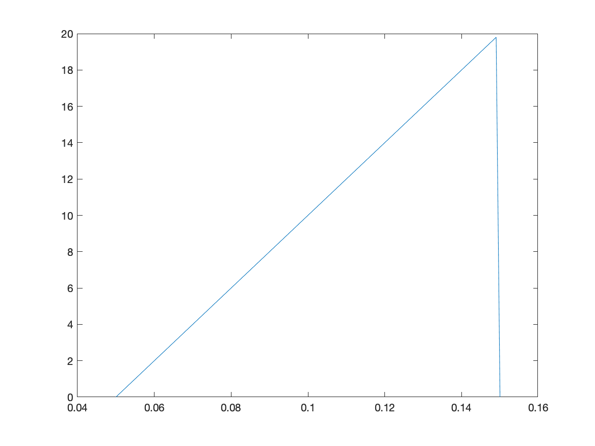
Figure B.2: A symmetric triangular distribution.
Refer to caption
(a) A symmetric triangular distribution
Refer to caption
(b) An increasing triangular distribution
Refer to caption
(c) A decreasing triangular distribution
Figure B.3: Integral on the left-hand side of (6.12) as function of LFL_{F} for various values of rr and β\beta for the symmetric triangular distribution in Figure B.2a
Refer to caption
(a) Integral vs. LFL_{F} varying β\beta in the base-case
Refer to caption
(b) Integral vs. LFL_{F} varying pp in the base-case
Refer to caption
(c) Integral vs. LFL_{F} varying qq in the base-case
Refer to caption
(d) Integral vs. LFL_{F} varying rr in the base-case
Figure B.4: Integral on the left-hand side of (6.12) as function of LFL_{F} for various values of rr and β\beta for the triangular distribution with increasing density in Figure B.2b
Refer to caption
(a) Integral vs. LFL_{F} varying β\beta in the base-case
Refer to caption
(b) Integral vs. LFL_{F} varying pp in the base-case
Refer to caption
(c) Integral vs. LFL_{F} varying qq in the base-case
Refer to caption
(d) Integral vs. LFL_{F} varying rr in the base-case
Figure B.5: Integral on the left-hand side of (6.12) as function of LFL_{F} for various values of rr and β\beta for the triangular distribution with decreasing density in Figure B.2c
Refer to caption
(a) Integral vs. LFL_{F} varying β\beta in the base-case
Refer to caption
(b) Integral vs. LFL_{F} varying pp in the base-case
Refer to caption
(c) Integral vs. LFL_{F} varying qq in the base-case
Refer to caption
(d) Integral vs. LFL_{F} varying rr in the base-case
Figure B.6: The sensitivity of the equilibrium mean service rate and the number of servers to various parameters for a symmetric triangular distribution
Refer to caption
(a) pp vs μ¯\bar{\mu}
Refer to caption
(b) qq vs μ¯\bar{\mu}
Refer to caption
(c) rr vs μ¯\bar{\mu}
Refer to caption
(d) pp vs NN
Refer to caption
(e) qq vs NN
Refer to caption
(f) rr vs NN
Figure B.7: The sensitivity of the equilibrium mean service rate and the number of servers to various parameters for a triangular distribution with increasing density
Refer to caption
(a) pp vs μ¯\bar{\mu}
Refer to caption
(b) qq vs μ¯\bar{\mu}
Refer to caption
(c) rr vs μ¯\bar{\mu}
Refer to caption
(d) pp vs NN
Refer to caption
(e) qq vs NN
Refer to caption
(f) rr vs NN
Figure B.8: The sensitivity of the equilibrium mean service rate and the number of servers to various parameters for a triangular distribution with decreasing density
Refer to caption
(a) pp vs μ¯\bar{\mu}
Refer to caption
(b) qq vs μ¯\bar{\mu}
Refer to caption
(c) rr vs μ¯\bar{\mu}
Refer to caption
(d) pp vs NN
Refer to caption
(e) qq vs NN
Refer to caption
(f) rr vs NN
Figure B.9: The sensitivity of the equilibrium mean service rate and the number of servers to staffing level β\beta for a symmetric triangular distribution
Refer to caption
(a) β\beta vs μ¯\bar{\mu}
Refer to caption
(b) β\beta vs NN
Figure B.10: The sensitivity of the equilibrium mean service rate and the number of servers to staffing level β\beta for a triangular distribution with increasing density
Refer to caption
(a) β\beta vs μ¯\bar{\mu}
Refer to caption
(b) β\beta vs NN
Figure B.11: The sensitivity of the equilibrium mean service rate and the number of servers to staffing level β\beta for a triangular distribution with decreasing density
Refer to caption
(a) β\beta vs μ¯\bar{\mu}
Refer to caption
(b) β\beta vs NN
Figure B.12: The equilibrium distributions for different parametric setups with a symmetric triangular distribution
Refer to caption
(a) p=−1,q=2,r=0.5,β=0.4p=-1,q=2,r=0.5,\beta=0.4
Refer to caption
(b) p=−0.6,q=2,r=0.5,β=0.4p=-0.6,q=2,r=0.5,\beta=0.4
Refer to caption
(c) p=−0.2,q=2,r=0.5,β=0.4p=-0.2,q=2,r=0.5,\beta=0.4
Refer to caption
(d) p=−1,q=3,r=0.5,β=0.4p=-1,q=3,r=0.5,\beta=0.4
Refer to caption
(e) p=−1,q=4,r=0.5,β=0.4p=-1,q=4,r=0.5,\beta=0.4
Refer to caption
(f) p=−1,q=5,r=0.5,β=0.4p=-1,q=5,r=0.5,\beta=0.4
Refer to caption
(g) p=−1,q=2,r=0.25,β=0.4p=-1,q=2,r=0.25,\beta=0.4
Refer to caption
(h) p=−1,q=2,r=0.75,β=0.4p=-1,q=2,r=0.75,\beta=0.4
Refer to caption
(i) p=−1,q=2,r=1,β=0.4p=-1,q=2,r=1,\beta=0.4
Refer to caption
(j) p=−1,q=2,r=0.5,β=0.2p=-1,q=2,r=0.5,\beta=0.2
Refer to caption
(k) p=−1,q=2,r=0.5,β=0.6p=-1,q=2,r=0.5,\beta=0.6
Refer to caption
(l) p=−1,q=2,r=0.5,β=0.8p=-1,q=2,r=0.5,\beta=0.8
Figure B.13: The equilibrium distributions for different parametric setups with a triangular distribution with an increasing density
Refer to caption
(a) p=−1,q=2,r=0.5,β=0.4p=-1,q=2,r=0.5,\beta=0.4
Refer to caption
(b) p=−0.6,q=2,r=0.5,β=0.4p=-0.6,q=2,r=0.5,\beta=0.4
Refer to caption
(c) p=−0.2,q=2,r=0.5,β=0.4p=-0.2,q=2,r=0.5,\beta=0.4
Refer to caption
(d) p=−1,q=3,r=0.5,β=0.4p=-1,q=3,r=0.5,\beta=0.4
Refer to caption
(e) p=−1,q=4,r=0.5,β=0.4p=-1,q=4,r=0.5,\beta=0.4
Refer to caption
(f) p=−1,q=5,r=0.5,β=0.4p=-1,q=5,r=0.5,\beta=0.4
Refer to caption
(g) p=−1,q=2,r=0.25,β=0.4p=-1,q=2,r=0.25,\beta=0.4
Refer to caption
(h) p=−1,q=2,r=0.75,β=0.4p=-1,q=2,r=0.75,\beta=0.4
Refer to caption
(i) p=−1,q=2,r=1,β=0.4p=-1,q=2,r=1,\beta=0.4
Refer to caption
(j) p=−1,q=2,r=0.5,β=0.2p=-1,q=2,r=0.5,\beta=0.2
Refer to caption
(k) p=−1,q=2,r=0.5,β=0.6p=-1,q=2,r=0.5,\beta=0.6
Refer to caption
(l) p=−1,q=2,r=0.5,β=0.8p=-1,q=2,r=0.5,\beta=0.8
Figure B.14: The equilibrium distributions for different parametric setups with a triangular distribution with an increasing density
Refer to caption
(a) p=−1,q=2,r=0.5,β=0.4p=-1,q=2,r=0.5,\beta=0.4
Refer to caption
(b) p=−0.6,q=2,r=0.5,β=0.4p=-0.6,q=2,r=0.5,\beta=0.4
Refer to caption
(c) p=−0.2,q=2,r=0.5,β=0.4p=-0.2,q=2,r=0.5,\beta=0.4
Refer to caption
(d) p=−1,q=3,r=0.5,β=0.4p=-1,q=3,r=0.5,\beta=0.4
Refer to caption
(e) p=−1,q=4,r=0.5,β=0.4p=-1,q=4,r=0.5,\beta=0.4
Refer to caption
(f) p=−1,q=5,r=0.5,β=0.4p=-1,q=5,r=0.5,\beta=0.4
Refer to caption
(g) p=−1,q=2,r=0.25,β=0.4p=-1,q=2,r=0.25,\beta=0.4
Refer to caption
(h) p=−1,q=2,r=0.75,β=0.4p=-1,q=2,r=0.75,\beta=0.4
Refer to caption
(i) p=−1,q=2,r=1,β=0.4p=-1,q=2,r=1,\beta=0.4
Refer to caption
(j) p=−1,q=2,r=0.5,β=0.2p=-1,q=2,r=0.5,\beta=0.2
Refer to caption
(k) p=−1,q=2,r=0.5,β=0.6p=-1,q=2,r=0.5,\beta=0.6
Refer to caption
(l) p=−1,q=2,r=0.5,β=0.8p=-1,q=2,r=0.5,\beta=0.8

References

  • [1] G. Allon and I. Gurvich (2010) Pricing and dimensioning competing large-scale service providers. Manufacturing and Service Operations Management 12 (3), pp. 449–469. Cited by: §2.
  • [2] M. Armony and A.R. Ward (2010) Fair dynamic routing in large-scale heterogeneous-service systems. Operations Research 3 (58), pp. 624–637. Cited by: §A.2, item 1, §1, §3.2.
  • [3] M. Armony (2005) Dynamic routing in large-scale service systems with heterogeneous servers. Queueing Systems 51 (3-4), pp. 287–329. Cited by: §1.
  • [4] M. Armony, G. Roels, and H. Song (2021) Capacity choice game in a multi-server queue: existence of a nash equilibrium. Naval Research Logistics 68 (5), pp. 663–678. Cited by: §2, §6.1.
  • [5] R. Atar, Y.Y. Shaki, and A. Shwartz (2011) A blind policy for equalizing cumulative idleness. Queueing Systems 67, pp. 275–293. Cited by: item 1, §1.
  • [6] R. Atar (2008) Central Limit Theorem for a Many-Server Queue with Random Service Rates. The Annals of Applied Probability 18 (4), pp. 1548–1568. Cited by: §1, Remark 4.3.
  • [7] E. Bayraktar, A. Budhiraja, and A. Cohen (2019) Rate Control Under Heavy Traffic with Strategic Servers. The Annals of Applied Probability 29 (1), pp. 1–35. Cited by: §2, §4.
  • [8] P. Billingsley (1999) Convergence of probability measures. Second edition, Wiley Series in Probability and Statistics: Probability and Statistics, John Wiley & Sons Inc., New York. Cited by: §A.4.
  • [9] S. Boyd and L. Vandenberghe (2004) Convex optimization. Cambridge University Press. Cited by: §A.5.
  • [10] S. Browne and W. Whitt (1995) Piecewise-linear diffusion processes. In Advances in queueing, Probab. Stochastics Ser., pp. 463–480. External Links: Review MathReviews Cited by: §6.1.
  • [11] B. Büke and W. Qin (2023) Many-server queues with random service rates in the Halfin-Whitt regime: a measure-valued process approach. Mathematics of Operations Research 48 (2), pp. 748–783. Cited by: §A.2, §A.2, §A.2, §A.2, §A.3, §A.3, §A.3, §A.5, §A.5, §1, §1, §3.2, §3.2, §3.2, §3.2, Remark 4.3.
  • [12] G. Cachon and P. Harker (2002) Competition and outsourcing with scale economies. Management Science 48 (10), pp. 1314–1333. Cited by: §2.
  • [13] G. Cachon and F. Zhang (2007) Obtaining fast service in a queueing system via performance-based allocation of demand. Management Science 53 (3), pp. 408–420. Cited by: §2.
  • [14] CallCentreHelper.com (2017) 7 Tricks That Call Centre Employees Play. Note: [Accessed 17-December-2024] External Links: Link Cited by: §1.
  • [15] Y. Cohen-Charash and P.E. Spector (2001) The role of justice in organizations: a meta-analysis. Organizational Behavior and Human Decision Processes 86 (2), pp. 278–321. Cited by: §1.
  • [16] J.A. Colquitt, D.E. Colon, M.J. Wesson, C.O.L.H. Porter, and K. Y. Ng (2001) Justice at the millenium: a meta-analytic review of 25 years of organizational justice research. Journal of Applied Psychology 86 (3), pp. 425–445. Cited by: §1.
  • [17] Deloitte (2017) Global Contact Center Survey. Technical report Deloitte. Cited by: §1.
  • [18] N. Gans, G. Koole, and A. Mandelbaum (2003) Telephone call centers: tutorial, review, and research prospects. Manufacturing and Service Operations Management 5 (2), pp. 79–141. Cited by: §1, §3.
  • [19] N. Gans, N. Liu, A. Mandelbaum, H. Shen, and H. Ye (2010) Service times in call centers: Agent heterogeneity and learning with some operational consequences. In Borrowing strength: Theory powering applications, Vol. 6, pp. 99–123. Cited by: §1.
  • [20] O. Garnett, A. Mandelbaum, and M. Reiman (2002) Designing a Call Center with Impatient Customers. Manufacturing & Service Operations Management 4 (3), pp. 208–227. Cited by: §3.
  • [21] S. Gilbert and Z. Weng (1998) Incentive Effects Favor Nonconsolidating Queues in a Service System : The Principal-Agent Perspective. Management Science 44 (12), pp. 1662–1669. Cited by: §2.
  • [22] Go4Customer (2021) What is Call Avoidance?. Note: [Accessed 17-December-2024] External Links: Link Cited by: §1.
  • [23] R. Gopalakrishnan, S. Doroudi, A. R. Ward, and A. Wierman (2016) Routing and staffing when servers are strategic. Operations Research 64 (4), pp. 1033–1050. Cited by: §A.5, §A.5, item 2, §1, §2, §3, §6.1, §6.1, §6.1, §6.2.
  • [24] R. Gopalakrishnan (2021) On the architecture of service systems when servers are strategic. Note: working paper, Smith School of Business, Queen’s University Cited by: §2, §6.1, §6.2.
  • [25] H. Gumbel (1960) Waiting lines with heterogeneous servers. Operations Research 8 (4), pp. 504–511. Cited by: §1, §1.
  • [26] I. Gurvich and W. Whitt (2009) Queue-and-idleness-ratio controls in many-server service systems. Mathematics of Operations Research 34, pp. 363–396. Cited by: §1.
  • [27] S. Halfin and H. Whitt (1981) Heavy-Traffic Limits for Queues with Many Exponential Serverss. Operations Research 29 (3), pp. 567–588. Cited by: §1.
  • [28] R. Hassin and M. Haviv (2003) To queue or not to queue: equilibrium behavior in queueing systems. Kluwer. Cited by: §2.
  • [29] R. Hassin (2020) Rational queueing. CRC Press. Cited by: §2.
  • [30] A. Jakubowski (1986) On the Skorokhod topology. Annales de l’institut Henri Poincare (B) Probability and Statistics 22 (3), pp. 263–285. Cited by: §A.4, Theorem A.5.
  • [31] E. Kalai, M. Kamien, and M. Rubinovitch (1992) Optimal Service Speeds in a Competitive Environment. Management Science 38 (8), pp. 1154–1163. Cited by: §2.
  • [32] G. Pang, R. Talreja, and W. Whitt (2007) Martingale proofs of many-server heavy-traffic limits for Markovian queues. Probability Surveys 4, pp. 193–267. Cited by: §A.2, §A.4.
  • [33] PWC (2018) Experience is everything: Here’s how to get it right. Technical report PWC. Note: Available at pwc.com/future-of-cx Cited by: §1.
  • [34] J. Reed and Y. Shaki (2015) A fair policy for the G/G​I/NG/GI/N Queue with Multiple Pools. Mathematics of Operations Research 40 (3), pp. 558–595. Cited by: item 1, §1.
  • [35] Statista Research Department (2020) Global call center market size 2020-2027. Technical report Statista. Cited by: §1.
  • [36] A.R. Ward and M. Armony (2013) Blind fair routing in large-scale service systems with heterogeneous customers and servers. Operations Research 1 (61), pp. 228–243. Cited by: §A.2, item 1, §1, §3.2.
  • [37] D. Zhan and A. R. Ward (2019) Staffing, routing, and payment to trade off speed and quality in large service systems. Operations Research. Cited by: §2.
  • [38] Y. Zhong, R. Gopalakrishnan, and A. Ward (2021) Behavior-aware queueing : the finite-buffer setting with many strategic servers. Note: submitted to Operations Research Cited by: §2.