跳到论文正文
W Papers独立论文阅读器 arXiv:2211.04093 论文正文 计算阅读时间 · 0%
引用这篇论文根据当前论文元数据生成,正式投稿前建议核对。


License: arXiv.org perpetual non-exclusive license
arXiv:2211.04093v3 [math.DG] 07 Jan 2026

Geometric rigidity of quasi-isometries in horospherical products

Tom Ferragut
August 11, 2026
Abstract

We prove that quasi-isometries of horospherical products of hyperbolic spaces are geometrically rigid in the sense that they are uniformly close to product maps, this is a generalization of the result obtained by Eskin, Fisher and Whyte in [EFW12]. Our work covers the case of solvable Lie groups of the form ℝ⋉(N1×N2)\mathbb{R}\ltimes(N_{1}\times N_{2}), where N1N_{1} and N2N_{2} are nilpotent Lie groups, and where the action on ℝ\mathbb{R} contracts the metric on N1N_{1} while extending it on N2N_{2}. We obtain new quasi-isometric invariants and classifications for these spaces.

Introduction

Let (X,dX)(X,d_{X}) and (Y,dY)(Y,d_{Y}) be two Gromov hyperbolic spaces. Their horospherical product, denoted by X⋈YX\bowtie Y is constructed by combining XX and YY, and lies in the direct product X×YX\times Y. It has no longer negative curvature, however its geometry is still very rigid (see Section 1.2 for the definition). This way of combining two hyperbolic spaces appeared to unify the construction of metric spaces such as Diestel-Leader graphs, treebolic spaces and Sol geometries, which are the horospherical products constructed out of a regular infinite tree or the hyperbolic plane ℍ2\mathbb{H}_{2}.

Quasi-isometric classification and existing rigidity results

In [Gro93], a mainstay of geometric group theory, Gromov points out the importance of quasi-isometric invariants in groups. The quasi-isometric classification of groups, or metric spaces, has since been a wide and prolific research domain (see [Kap14] for a nice survey on this topic). For the family of solvable groups, there are still a lot of open cases.

The first result was obtained in [FM98] where Farb and Mosher provided a quasi-isometric classification of solvable Baumslag-Solitar groups BS⁡(1,n)\mathrm{BS}(1,n). Then Eskin, Fisher and Whyte obtained the quasi-isometric classification of lamplighter groups and Sol geometries in [EFW12] and [EFW13]. In both the works [FM98] and [EFW12], the horospherical product construction of their respective groups is crucial in their proofs.

The paper [EFW12] also permitted to answer a question asked by Woess in [SW90] about the existence of vertex-transitive graphs not quasi-isometric to any Cayley graph. Eskin, Fisher and Whyte showed that when mm and nn are coprime integers, the Diestel-Leader graphs Tm⋈TnT_{m}\bowtie T_{n} are such graphs.

Throughout [Pen11I], [Pen11II] and [Dym09], using similar methods as in [EFW12] and [EFW13], Peng and Dymarz generalized the description of the quasi-isometries for Lie groups of the form ℝ⋉ℝp\mathbb{R}\ltimes\mathbb{R}^{p}. In [Pen11I] and [Pen11II], Peng proved that a subgroup of finite index of the quasi-isometry group of Lie groups of the form ℝm⋉ℝn\mathbb{R}^{m}\ltimes\mathbb{R}^{n} is a product of groups of bilipschitz maps.

Statement of results

The main goal of our work is to generalize the methods and techniques developed by Eskin, Fisher and Whyte to a wider set of horospherical products X⋈YX\bowtie Y. In order to do that, the spaces XX and YY are endowed with appropriate measures (see Definition 3.1). Once endowed with suitable measures, XX and YY are called horopointed admissible spaces.

To be more precise let XX (respectively X′X^{\prime}, YY, Y′Y^{\prime}) be a horopointed admissible space with exponential growth parameter mm (respectively m′m^{\prime}, nn, n′n^{\prime}). When XX is a regular tree, the parameter mm is related to the degree of XX. When XX is a negatively curved Lie group ℝ⋉AN\mathbb{R}\ltimes_{A}N, the parameter mm is tr⁡(A)\mathrm{tr}(A), the trace of AA.

Let Φ:X⋈Y→X′⋈Y′\Phi:X\bowtie Y\to X^{\prime}\bowtie Y^{\prime} be a quasi-isometry. The map Φ\Phi is called a product map if and only if there exist two maps ΦX:X→X\Phi^{X}:X\to X (or ΦX:X→Y\Phi^{X}:X\to Y) and ΦY:Y→Y\Phi^{Y}:Y\to Y (or ΦY:Y→X\Phi^{Y}:Y\to X) such that for all (x,y)∈X⋈Y(x,y)\in X\bowtie Y we have either:

Φ⁡(x,y)=(ΦX​(x),ΦY​(y))orΦ⁡(x,y)=(ΦY​(y),ΦX​(x)).\displaystyle\Phi(x,y)=\left(\Phi^{X}(x),\Phi^{Y}(y)\right)\quad\text{or}\quad\Phi(x,y)=\left(\Phi^{Y}(y),\Phi^{X}(x)\right).

Our main theorem states that, when m>nm>n and m′>n′m^{\prime}>n^{\prime}, any quasi-isometry Φ:X⋈Y→X′⋈Y′\Phi:X\bowtie Y\to X^{\prime}\bowtie Y^{\prime} is close to a product map.

Theorem A (Geometric rigidity).


Let XX, X′X^{\prime}, YY and Y′Y^{\prime} be horo-pointed admissible measured metric spaces with m>nm>n and m′>n′m^{\prime}>n^{\prime} and let Φ:X⋈Y→X′⋈Y′\Phi:X\bowtie Y\to X^{\prime}\bowtie Y^{\prime} be a quasi-isometry. Then there exist two quasi-isometries ΦX:X→X′\Phi^{X}:X\to X^{\prime} and ΦY:Y→Y′\Phi^{Y}:Y\to Y^{\prime} such that:

d⋈​(Φ,(ΦX,ΦY))<+∞.\displaystyle d_{\bowtie}\left(\Phi,\left(\Phi^{X},\Phi^{Y}\right)\right)<+\infty.

This is a generalization of Theorems 2.12.1 and 2.32.3 of [EFW12]. While completing the proof of this result, we obtained a first quasi-isometry invariant in horospherical products.

Theorem B.

When m>nm>n, the parameter mn\frac{m}{n} is a quasi-isometry invariant.

Let ℝ⋉A1N1\mathbb{R}\ltimes_{A_{1}}N_{1} and ℝ⋉A2N2\mathbb{R}\ltimes_{A_{2}}N_{2} be two simply connected, negatively curved, solvable Lie groups (also called Heintze groups). In Chapter 5 we show that this couple of Heintze groups is admissible, and that the condition m>nm>n is equivalent to t​r​(A1)>t​r​(A2)tr(A_{1})>tr(A_{2}). We obtain a necessary condition for the existence of a quasi-isometry on solvable Lie groups. The horospherical product of these two Heintze groups is isomorphic to

G:=ℝ⋉Diag⁡(A1,−A2)(N1×N2),\displaystyle G:=\mathbb{R}\ltimes_{\mathrm{Diag}(A_{1},-A_{2})}(N_{1}\times N_{2}),

defined by the diagonal action of ℝ\mathbb{R}, t↦(exp⁡(t​A1),exp⁡(−t​A2))t\mapsto(\exp(tA_{1}),\exp(-tA_{2})) on N1×N2N_{1}\times N_{2}.

We say that GG is Carnot-Sol type if N1N_{1} and N2N_{2} are Carnot groups and if A1A_{1} and A2A_{2} are multiples of Carnot derivations of N1N_{1} and N2N_{2} respectively. In the literature (see [Pan89] for example), Carnot type stands for Lie groups with N2={1}N_{2}=\{1\}. Here we extend the denominations to non-hyperbolic Lie groups.

Using the previous quasi-isometry invariants we obtain the following quasi-isometry classification.

Theorem C.

Let G=ℝ⋉Diag⁡(A1,−A2)(N1×N2)G=\mathbb{R}\ltimes_{\mathrm{Diag}(A_{1},-A_{2})}(N_{1}\times N_{2}) and G′=ℝ⋉Diag⁡(A1′,−A2′)(N1′×N2′)G^{\prime}=\mathbb{R}\ltimes_{\mathrm{Diag}(A_{1}^{\prime},-A_{2}^{\prime})}(N_{1}^{\prime}\times N_{2}^{\prime}) be Carnot-Sol type, non-unimodular Lie groups, then

G and G′ are quasi-isometric⇔G and G′ are isomorphic.G\text{ and }G^{\prime}\text{ are quasi-isometric}\quad\Leftrightarrow\quad G\text{ and }G^{\prime}\text{ are isomorphic}. (1)

The case where N2={1}N_{2}=\{1\} is treated in Corollary 12.4 of [Pan89].

Recall that a group GG is called metabelian if [G,G][G,G] is abelian (when both N1N_{1} and N2N_{2} are euclidean spaces). In this case, a similar quasi-isometry classification is deduced from the work of Peng [Pen11I] and [Pen11II]. Both the quasi-isometry classification for the metabelian groups and for Carnot-Sol type groups are special cases of the conjecture 19.11319.113 of [Cor18] that we recall.

Conjecture 0.1.

Let SS and S′S^{\prime} be completely solvable Lie groups. Then SS and S′S^{\prime} are quasi-isometric if and only if they are isomorphic.

Classifying completely solvable Lie groups up to quasi-isometry would yield the quasi-isometry classification of all connected Lie groups, see [Cor12].

For i∈{1,2}i\in\{1,2\}, let NiN_{i} and Ni′N_{i}^{\prime} be two simply connected, nilpotent groups and let Ai∈Lie⁡(Ni)A_{i}\in\mathrm{Lie}(N_{i}) and Ai′∈Lie⁡(Ni′)A_{i}^{\prime}\in\mathrm{Lie}(N_{i}^{\prime}) be derivations. Let G:=ℝ⋉Diag⁡(A1,−A2)(N1×N2)G:=\mathbb{R}\ltimes_{\mathrm{Diag}(A_{1},-A_{2})}(N_{1}\times N_{2}) and G′:=ℝ⋉Diag⁡(A1′,−A2′)(N1′×N2′)G^{\prime}:=\mathbb{R}\ltimes_{\mathrm{Diag}(A_{1}^{\prime},-A_{2}^{\prime})}(N_{1}^{\prime}\times N_{2}^{\prime}). In this general setting of horospherical products of Heintze groups we have the following necessary conditions for being quasi-isometric.

Proposition D.

Let us assume that tr⁡(A1)>tr⁡(A2)\mathrm{tr}(A_{1})>\mathrm{tr}(A_{2}) and tr⁡(A1′)>tr⁡(A2′)\mathrm{tr}(A_{1}^{\prime})>\mathrm{tr}(A_{2}^{\prime}). If GG and G′G^{\prime} are quasi-isometric, then we have that for i∈{1,2}i\in\{1,2\}

  1. 1.

    NiN_{i} and Ni′N_{i}^{\prime} are bilipschitz;

  2. 2.

    AiA_{i} and tr⁡(A1)tr⁡(A1′)​Ai′\frac{\mathrm{tr}(A_{1})}{\mathrm{tr}(A_{1}^{\prime})}A_{i}^{\prime} share the same characteristic polynomial.

With the same setting, using the geometric rigidity on self quasi-isometries of this family of solvable Lie groups, we provide a characterisation of their quasi-isometry group.

Recall that for FF a metric space, QI⁡(F)/∼\mathrm{QI}(F)\big/\mathord{\sim} is the group of self quasi-isometries of FF, up to finite distance. (This equivalence relation is required since a quasi-isometry only has a coarse inverse.) Recall also that Bilip⁡(F)\mathrm{Bilip}(F) stands for the group of self bi-Lipschitz maps of FF. Then we have:

Theorem E.

If t​r​(A1)≠t​r​(A2)\penalty\ tr(A_{1})\neq tr(A_{2}):

QI⁡(ℝ⋉Diag⁡(A1,−A2)(N1×N2))/∼=Bilip⁡(N1)×Bilip.(N2)\displaystyle\mathrm{QI}\left(\mathbb{R}\ltimes_{\mathrm{Diag}(A_{1},-A_{2})}(N_{1}\times N_{2})\right)\big/\mathord{\sim}=\mathrm{Bilip}\left(N_{1}\right)\times\mathrm{Bilip}.\left(N_{2}\right) (2)

Here we choose the horospherical product metric on ℝ⋉Diag⁡(A1,−A2)(N1×N2)\mathbb{R}\ltimes_{\mathrm{Diag}(A_{1},-A_{2})}(N_{1}\times N_{2}).

In the course of this proof we also obtain that any self quasi-isometry of ℝ⋉Diag⁡(A1,−A2)(N1×N2)\mathbb{R}\ltimes_{\mathrm{Diag}(A_{1},-A_{2})}(N_{1}\times N_{2}) is a rough isometry. Le Donne, Pallier and Xie proved in [DPX22] that when you change the left-invariant Riemannian metric of one of these solvable Lie groups, the identity map is a rough similarity. Hence self quasi-isometries are rough isometries with respect to any left-invariant distances.

Outline of the proof

Let XX and YY be two Gromov hyperbolic spaces, and let βX:X→ℝ\beta_{X}:X\to\mathbb{R} and βY:Y→ℝ\beta_{Y}:Y\to\mathbb{R} be two Busemann functions. We call height functions hXh_{X} and hYh_{Y} the opposite of the Busemann functions. The horospherical product of XX and YY, denoted by X⋈YX\bowtie Y, is defined as the set of points in X×YX\times Y such that the two Busemann functions (or the height functions) add up to zero.

X⋈Y:={(x,y)∈X×Y∣βX​(x)+βY​(y)=0}.X\bowtie Y:=\{(x,y)\in X\times Y\mid\beta_{X}(x)+\beta_{Y}(y)=0\}.

A Busemann function is associated with a unique point on the boundary. We call any geodesic ray in the equivalence class of this point a vertical geodesic ray.

In order to generalize the proof of Eskin, Fisher and Whyte developed in [EFW12] and [EFW13], the horospherical products have to be equipped with appropriate measures presented in Definition 3.1.

Briefly speaking, for the measured space (X,μX)(X,\mu^{X}), the measure μX\mu^{X} must verify three assumptions. Assumption (E​1)(E1) allows us to disintegrate μX\mu^{X} on its horospheres, assumption (E​2)(E2) provides us with a bounded geometry on horospheres and (E​3)(E3) ensures an exponential contraction (of exponent mm) of the horospheres’ measures in the upward vertical direction.

Let XX (respectively X′X^{\prime}, YY, Y′Y^{\prime}) be a horopointed admissible space with exponential growth parameter mm (respectively m′m^{\prime}, nn, n′n^{\prime}).

Most of this paper focuses on proving Theorem A. To do so we will use three major tools:

  1. ∙\bullet

    The coarse vertical quadrilaterals, which are realised by four points (the vertices) whose neighbourhoods are linked by vertical geodesics (the edges). In Lemma 2.11, we show that coarse vertical quadrilaterals are rigid: two of the four points almost share the same XX-coordinate and the two other almost share the same YY-coordinate.

  2. ∙\bullet

    Box Tilings of different scales for X⋈YX\bowtie Y, suitable for the vertical flow. The boxes correspond to euclidean rectangular cuboid in the Sol geometry.

  3. ∙\bullet

    The coarse differentiation: given a quasi-isometry Φ:X⋈Y→X′⋈Y′\Phi:X\bowtie Y\to X^{\prime}\bowtie Y^{\prime}, there exists a suitable scale RR for the box tilling of X⋈YX\bowtie Y. Suitable here means that the image by Φ\Phi of most vertical geodesic segments of length RR are close to a vertical geodesic segment.

With these tools, the proof can be summarized as follows. Let Φ:X⋈Y→X′⋈Y′\Phi:X\bowtie Y\to X^{\prime}\bowtie Y^{\prime} be a quasi-isometry.

Step 1

By the coarse differentiation, there exists a scale RR such that in the box tilling at scale RR of X⋈YX\bowtie Y, the quasi-isometry Φ\Phi mostly preserve the vertical direction on most of the boxes at scale RR. It means that on most of the boxes, most vertical geodesic segments are sent close to a vertical geodesic segment by Φ\Phi.

Step 2

Then in most of the boxes at scale RR, most of the vertical quadrilateral are sent close to vertical quadrilateral by Φ\Phi. Therefore, by the rigidity property of these configurations, on most of the boxes ℬ\mathcal{B} the quasi-isometry Φ\Phi is close to a product map Φ^|ℬ=(Φ^X,Φ^Y)\hat{\Phi}_{|\mathcal{B}}=\left(\hat{\Phi}^{X},\hat{\Phi}^{Y}\right) or (Φ^Y,Φ^X)\left(\hat{\Phi}^{Y},\hat{\Phi}^{X}\right).

Step 3

If m>nm>n and m′>n′m^{\prime}>n^{\prime} then all product maps have the form Φ^ℬ=(ΦX,ΦY)\hat{\Phi}_{\mathcal{B}}=\left(\Phi^{X},\Phi^{Y}\right). Therefore by gluing them together, we show that there exists L>>RL>>R such that on all boxes at scale LL, Φ\Phi is close to a product map Φ^=(ΦX,ΦY)\hat{\Phi}=\left(\Phi^{X},\Phi^{Y}\right).

Step 4

We show that Φ\Phi quasi-respect the height, then we use this last result on Φ−1\Phi^{-1} to show that Φ\Phi send all vertical geodesics close to vertical geodesics. Therefore all vertical quadrilateral configurations are preserved by Φ\Phi, hence Φ\Phi itself is close to a product map on all X⋈YX\bowtie Y.

A major technical issue in this proof is to manage the notion of "almost all" vertical geodesic segments having a certain property. The disintegrable measure μ\mu of assumption (E​1)(E1) is not suited for this role since it concentrates the measure of a box on its bottom part. Therefore we introduce another disintegrable measure λ\lambda, constructed from μ\mu, which (almost) equally weights the level-sets of the height function hh in boxes.

Such a measure λX\lambda^{X} on XX, together with a similar measure λY\lambda^{Y} on YY, allows us to define a suitable measure (later denoted by η\eta) on the family of vertical geodesics contained in a box ℬ⊂X⋈Y\mathcal{B}\subset X\bowtie Y.

The geometric rigidity has useful consequences when we understand the boundaries of XX and YY. In this case, Theorem A leads to a description of the quasi-isometry-group of X⋈YX\bowtie Y. In the last section of this paper, we detail such a description for the horospherical product of two Heintze groups.

Organization of the paper

This work, about the geometric rigidity of quasi-isometries between two horospherical products, is organized as followed.

  1. ∙\bullet

    In Section 2 we display the coarse differentiation in our context, and we discuss particular quadrilateral configurations of X⋈YX\bowtie Y.

  2. ∙\bullet

    Section 3 focuses on developing all the measure theoretical tools required to achieve the rigidity results.

  3. ∙\bullet

    Then, in Section 4, we follow the structure of the proof proposed by Eskin, Fisher and Whyte in [EFW12], invoking technical tools of previous chapters when required.

  4. ∙\bullet

    In the last section we present an application of our theorem by providing new quasi-isometric classifications for some families of solvable Lie groups. We also provide a description of the quasi-isometry group of a wider family of solvable Lie groups.

Acknowledgement

This work was supported by the University of Montpellier, as well as by the Japan Society for the Promotion of Science (JSPS) and the ERC of Enrico Le Donne.

I am deeply grateful to my advisors, Jeremie Brieussel and Constantin Vernicos, for their guidance, for their many reviews and comments. I also wish to thank Xiangdong Xie for the early and stimulating discussions regarding the paper of Eskin, Fisher and Whyte. My thanks extend to Ryokichi Tanaka and Gabriel Pallier for their detailed explanations of the implications of geometric rigidity in the context of Lie groups. Lastly, I am particularly grateful to the reviewer for their meticulous reading, detailed feedback, and thoughtful suggestions, which greatly improved the quality of this paper.

1 Context

1.1 Gromov hyperbolic, Busemann spaces

Let δ>0\delta>0, and let (X,dX)(X,d_{X}) and (Y,dY)(Y,d_{Y}) be two δ\delta-hyperbolic spaces (See [GH90] or chap.III H. p.399 of [BH99] for more details on Gromov hyperbolic spaces). We present here the context in which we will construct our horospherical product. We require that XX and YY are both proper, geodesically complete, Busemann spaces.

  • •

    A metric space is called proper if all closed metric balls are compact.

  • •

    A geodesic line, respectively ray, segment, of XX is the isometric image of a Euclidean line, respectively half Euclidean line, interval, in XX. We denote by [x1,x2][x_{1},x_{2}] a geodesic segment linking x1∈Xx_{1}\in X to x2∈Xx_{2}\in X.

  • •

    A metric space XX is called geodesically complete if all geodesics are infinitely extendable.

  • •

    A metric space is called Busemann if the distance between any couple of geodesics parametrized by arclength is a convex function. (See Chap.8 and Chap.12 of [Pap04] for more details on Busemann spaces.)

An important property of Gromov hyperbolic spaces is that they admit a nice compactification thanks to their Gromov boundary. We call two geodesic rays of XX equivalent if their images are at finite Hausdorff distance. Let w∈Xw\in X be a base point. We define ∂wX\partial_{w}X, the Gromov boundary of XX, as the set of equivalence classes of geodesic rays starting from ww. While ∂wX\partial_{w}X as a set depends on the choice of the base point ww, it is topologically independent of ww under the cone topology. We denote the Gromov boundary simply by ∂X\partial X when the choice of ww does not matter topologically. The cone topology on X∪∂XX\cup\partial X restricts to the natural topology on XX, and with this topology, X∪∂XX\cup\partial X is compact (see [BH99] for further details on the cone topology). In this context, the Gromov boundary coincides with the visual boundary.

Let us fix a point a∈∂Xa\in\partial X on the boundary. We call vertical geodesic ray, respectively vertical geodesic line, any geodesic ray in the equivalence class aa, respectively any geodesic line with one of its half-lines in aa. The study of these specific geodesic rays is central in this work.
The Busemann assumption removes some technical difficulties in a significant number of proofs in this work. If XX is a Busemann space in addition to being Gromov hyperbolic, for all x∈Xx\in X there exists a unique vertical geodesic ray, denoted by VxV_{x}, starting at xx. In fact the distance between two vertical geodesics starting at xx is a convex and bounded function, hence decreasing and therefore constant equal to 00.
The construction of the horospherical product of two Gromov hyperbolic space XX and YY requires the so called Busemann functions. Their definition is simplified by the Busemann assumption. Let us consider ∂X\partial X, the Gromov boundary of XX (which, in this setting, is the same as the visual boundary). Both the boundary ∂X\partial X and X∪∂XX\cup\partial X, endowed with the natural Hausdorff topology, are compact. Then, given a∈∂Xa\in\partial X a point on the boundary, and w∈Xw\in X a base point, we define a Busemann function β(a,w)\beta_{(a,w)} with respect to aa and ww. Let VwV_{w} be the unique vertical geodesic ray starting from ww.

∀x∈X,β(a,w)​(x):=lim supt→+∞(d⁡(x,Vw​(t))−t).\forall\ x\in X,\ \beta_{(a,w)}(x):=\limsup\limits_{t\rightarrow+\infty}(d(x,V_{w}(t))-t).

In all our results, XX and YY will be proper, geodesically complete, Gromov hyperbolic, Busemann spaces, with some additional assumption from time to time.

1.2 Horospherical products

Let aX∈∂X,aY∈∂Ya^{X}\in\partial X,a^{Y}\in\partial Y be points on the boundaries and let wX∈X,wY∈Yw^{X}\in X,w^{Y}\in Y be base points. Let us denote by hX:=−β(aX,wX)h^{X}:=-\beta_{\left(a^{X},w^{X}\right)} and hY:=−β(aY,wY)h^{Y}:=-\beta_{\left(a^{Y},w^{Y}\right)} the two corresponding height functions. The horospherical product of XX and YY, relatively to (aX,wX)\left(a^{X},w^{X}\right) and (aY,wY)\left(a^{Y},w^{Y}\right) , denoted by X⋈YX\bowtie Y is defined by:

X⋈Y:={(x,y)∈X×Y∣hX​(x)+hY​(y)=0}.\displaystyle X\bowtie Y:=\left\{(x,y)\in X\times Y\mid h^{X}(x)+h^{Y}(y)=0\right\}.

The set X⋈YX\bowtie Y, can be seen as a diagonal in X×YX\times Y. It is constructed by gluing XX with an upside down copy of YY along their respective horospheres. This construction, illustrated in Figure 1, can also be seen as the union of the direct products between opposite horospheres in XX and YY

X⋈Y=⨆z∈ℝXz×Y−z.\displaystyle X\bowtie Y=\bigsqcup\limits_{z\in\mathbb{R}}X_{z}\times Y_{-z}.
Refer to caption
Figure 1: Horospherical product X⋈YX\bowtie Y.

From now on, with a slight abuse, we omit the reference to the base points and points on the boundaries in the construction of the horospherical product.

To study the geometry of a horospherical product X⋈YX\bowtie Y, we make additional assumptions on XX and YY. We require them to be Gromov hyperbolic, Busemann, geodesically complete and proper metric spaces.

  1. 1.

    XX is geodesically complete if and only if all geodesic segments of XX can be extended into a geodesic bi-infinite line.

  2. 2.

    XX is proper if and only if all closed metric balls of XX are compact.

If XX and YY satisfy these two additional conditions, the horospherical product X⋈YX\bowtie Y is connected (see Property 3.11 of [Fer20]).

Example 1.1.

Let XX be a Gromov hyperbolic, Busemann, geodesically complete and proper metric space. Then X⋈ℝX\bowtie\mathbb{R} is isometric to XX. In particular, if VY\penalty\ V^{Y} is a vertical geodesic line of Y\penalty\ Y, X⋈VYX\bowtie V^{Y} is an isometric embedding of XX in X⋈YX\bowtie Y.

The three (non-trivial) first examples of horospherical products appeared independently in the literature. They correspond to the case where XX and YY are either a regular infinite tree TmT_{m} of degree mm or the hyperbolic plane ℍ2\mathbb{H}^{2}.

  1. 1.

    Tm⋈TnT_{m}\bowtie T_{n} is the Diestel-Leader graph DL⁡(m,n)\mathrm{DL}(m,n). When m=nm=n, this horospherical product is a Cayley graph of the lamplighter group ℤ≀ℤm\mathbb{Z}\wr\mathbb{Z}_{m}. See Figure 2 for a subset of T3⋈T3T_{3}\bowtie T_{3}.

  2. 2.

    ℍ2,m⋈ℍ2,n\mathbb{H}^{2,m}\bowtie\mathbb{H}^{2,n} is the Lie group ℝ⋉(m,n)ℝ2=Sol⁡(m,n)\mathbb{R}\ltimes_{(m,n)}\mathbb{R}^{2}=\mathrm{Sol}(m,n), one of the eight Thurston geometries when m=nm=n. By ℍ2,m\mathbb{H}^{2,m} we mean the manifold ℝ2\mathbb{R}^{2} endowed with the infinitesimal Riemannian metric d​s2=e−2​m​z​d​x2+d​z2\mathrm{d}s^{2}=e^{-2mz}\mathrm{d}x^{2}+\mathrm{d}z^{2}. The action associated to the aforementioned semi-direct product is described by (z,(x,y))↦(em​z​x,e−n​z​y)(z,(x,y))\mapsto\left(e^{mz}x,e^{-nz}y\right).

  3. 3.

    Tm⋈ℍ2T_{m}\bowtie\mathbb{H}_{2} is a Cayley 22-complex of the Baumslag-Solitar group BS⁡(1,m)\mathrm{BS}(1,m).

Refer to caption
Figure 2: Small neighbourhood in T3⋈T3T_{3}\bowtie T_{3}.

The awareness of them being identically constructed from Gromov hyperbolic spaces came later, and a survey on these three examples is provided by Wolfgang Woess in [Woe13].

An other approach, is to consider the hyperbolic plane ℍ2,m\mathbb{H}^{2,m} as the affine Lie group ℝ⋉mℝ\mathbb{R}\ltimes_{m}\mathbb{R} with action by multiplication (z,x)↦em​z​x(z,x)\mapsto e^{mz}x, and the Sol geometry Sol(m,n)(m,n) as the Lie group ℝ⋉(m,n)ℝ2\mathbb{R}\ltimes_{(m,n)}\mathbb{R}^{2}. In this context we have that (ℝ⋉mℝ)⋈(ℝ⋉nℝ)=ℝ⋉(m,n)ℝ2(\mathbb{R}\ltimes_{m}\mathbb{R})\bowtie(\mathbb{R}\ltimes_{n}\mathbb{R})=\mathbb{R}\ltimes_{(m,n)}\mathbb{R}^{2}. The natural next step, is to consider which Lie group can be taken as a component in a horospherical product.

A Heintze group is a Lie group of the form ℝ⋉AN\mathbb{R}\ltimes_{A}N with NN a nilpotent Lie group, with AA the derivation of the Lie algebra and where all eigenvalues of AA have positive real part. Heintze proved in [Hei74] that any simply connected, negatively curved solvable Lie group is isomorphic to a Heintze group.

Moreover, a Busemann metric space is simply connected, hence any Gromov hyperbolic, Busemann Lie group is isomorphic to a Heintze group. Consequently, Heintze groups are natural candidates for the two components from which a horospherical product is constructed. Let ℝ⋉A1N1\mathbb{R}\ltimes_{A_{1}}N_{1} and ℝ⋉A2N2\mathbb{R}\ltimes_{A_{2}}N_{2} be two Heintze groups, we have

(ℝ⋉A1N1)⋈(ℝ⋉A1N1)=ℝ⋉Diag⁡(A1,−A2)(N1×N2),\displaystyle\left(\mathbb{R}\ltimes_{A_{1}}N_{1}\right)\bowtie\left(\mathbb{R}\ltimes_{A_{1}}N_{1}\right)=\mathbb{R}\ltimes_{\mathrm{Diag}(A_{1},-A_{2})}(N_{1}\times N_{2}),

where Diag⁡(A1,−A2)\mathrm{Diag}(A_{1},-A_{2}) is the block diagonal matrix containing A1A_{1} and −A2-A_{2} on its diagonal.

In his paper [Xie14], Xie classifies the subfamily of all negatively curved Lie groups ℝ⋉ℝn\mathbb{R}\ltimes\mathbb{R}^{n} up to quasi-isometry. In Chapter 5, we provide a description of the quasi-isometry group of the horospherical product of two Heintze groups, namely the solvable Lie groups ℝ⋉Diag⁡(A1,−A2)(N1×N2)\mathbb{R}\ltimes_{\mathrm{Diag}(A_{1},-A_{2})}(N_{1}\times N_{2}).

1.3 Settings

In this chapter we recall some material about horospherical products.

In order to lighten the notations, we will not fully describe the multiplicative and additive constants involved in inequalities. We will use the following notations instead.

Notation 1.2.

Let A,B∈ℝA,B\in\mathbb{R} and ee a parameter (set, real numbers, …). Let us denote:

  1. 1.

    A⪯eBA\preceq_{e}B if and only if there exists a constant M⁡(e)M(e) depending only on ee such that A≤M⁡(e)​BA\leq M(e)B.

  2. 2.

    A≍eBA\asymp_{e}B if and only if B⪯eA⪯eBB\preceq_{e}A\preceq_{e}B.

If the constant MM is a specific integer such as 22, we will simply denote A⪯BA\preceq B, and similarly A⪰BA\succeq B, A≍BA\asymp B. The notation ⪯e\preceq_{e} might also appear for parameters in several results of this paper. In this context it means that there exists a constant depending only on ee such that the implied result holds.

A metric space is called geodesically complete if all its geodesic segments can be extended into geodesic lines, therefore when the space is also Gromov hyperbolic and Busemann space, with respect to a∈∂Xa\in\partial X, any point is included in a vertical geodesic line (not necessarily unique).

We define the relative distance between two points x1x_{1} and x2x_{2} of XX as:

dr​(x1,x2)=d⁡(x1,x2)−Δ​h​(x1,x2).d_{r}\left(x_{1},x_{2}\right)=d\left(x_{1},x_{2}\right)-\Delta h\left(x_{1},x_{2}\right).

It can be understood as the distance along a level-set of the Busemann function. Let us recall Lemma 4.7 of [Fer20].

Lemma 1.3.


Let XX be a proper, δ\delta-hyperbolic, Busemann space. Let V1V_{1} and V2V_{2} be two vertical geodesics of HH. Let t1,t2∈ℝt_{1},t_{2}\in\mathbb{R} and let us denote D:=12​dr​(V1​(t1),V2​(t2))D:=\frac{1}{2}d_{r}\big(V_{1}(t_{1}),V_{2}(t_{2})\big). Then for all t∈[0,D]t\in\left[0,D\right]

|dr​(V1​(t1+D−t),V2​(t1+D−t))−2​t|≤288​δ.\left|d_{r}\big(V_{1}(t_{1}+D-t),V_{2}(t_{1}+D-t)\big)-2t\right|\leq 288\delta. (3)
Corollary 1.4.

Let V1V_{1}, V2V_{2} be two vertical geodesics of XX. Then there exists a height hdiv​(V1,V2)∈ℝh_{\mathrm{div}}(V_{1},V_{2})\in\mathbb{R} from which V1V_{1} and V2V_{2} diverge from each other:

  1. 1.

    ∀t≥hdiv​(V1,V2)\forall t\geq h_{\mathrm{div}}(V_{1},V_{2}), d(V1(t),V2(t))⪯δ1d\big(V_{1}(t),V_{2}(t)\big)\preceq_{\delta}1;

  2. 2.

    ∀t≤hdiv​(V1,V2)\forall t\leq h_{\mathrm{div}}(V_{1},V_{2}), |d(V1(t),V2(t))−2(hdiv(V1,V2)−t)|⪯δ1\left|d\big(V_{1}(t),V_{2}(t)\big)-2\left(h_{\mathrm{div}}(V_{1},V_{2})-t\right)\right|\preceq_{\delta}1.

This corollary is illustrated in Figure 3. We also have a more quantitative version.

Refer to caption
Figure 3: Figure of Lemma 1.4.
Lemma 1.5 (Lemma 4.3 of [Fer20]).

Let HH be a δ\delta-hyperbolic and Busemann metric space, let xx and yy be two elements of HH such that h⁡(x)≤h⁡(y)h(x)\leq h(y), and let α\alpha be a geodesic linking xx to yy. Let us denote z=α⁡(Δ​h​(x,y)+12​dr​(x,y))z=\alpha\left(\Delta h(x,y)+\frac{1}{2}d_{r}(x,y)\right), x1:=Vx​(h⁡(y)+12​dr​(x,y))x_{1}:=V_{x}\left(h(y)+\frac{1}{2}d_{r}(x,y)\right) the point of VxV_{x} at height h⁡(y)+12​dr​(x,y)h(y)+\frac{1}{2}d_{r}(x,y) and y1:=Vy​(h⁡(y)+12​dr​(x,y))y_{1}:=V_{y}\left(h(y)+\frac{1}{2}d_{r}(x,y)\right) the point of VyV_{y} at the same height h⁡(y)+12​dr​(x,y)h(y)+\frac{1}{2}d_{r}(x,y). Then we have:

  1. 1.

    supp∈α(h⁡(p))≥h⁡(y)+12​dr​(x,y)−96​δ\sup\limits_{p\in\alpha}\big(h(p)\big)\geq h(y)+\frac{1}{2}d_{r}(x,y)-96\delta;

  2. 2.

    d⁡(z,x1)≤144​δd\left(z,x_{1}\right)\leq 144\delta;

  3. 3.

    d⁡(z,y1)≤144​δd\left(z,y_{1}\right)\leq 144\delta;

  4. 4.

    d⁡(x1,y1)≤288​δd\left(x_{1},y_{1}\right)\leq 288\delta.

We list here some notations we will use in later sections.

Notation 1.6.

Let XX be a proper, geodesically complete, δ\delta-hyperbolic, Busemann space.

  1. 1.

    Let us denote the rr-neighbourhood of UU for all U⊂XU\subset X and for all r≥0r\geq 0 by

    𝒩r​(U):={x∈X∣d⁡(x,U)≤r}.\mathcal{N}_{r}(U):=\{x\in X\mid d(x,U)\leq r\}. (4)
  2. 2.

    For all x∈Xx\in X let us denote by VxV_{x} the unique vertical geodesic ray such that Vx​(0)=xV_{x}(0)=x.

  3. 3.

    For a subset A⊂XA\subset X, let us denote

    h−​(A):=infx∈A(h⁡(x));h+​(A):=supx∈A(h⁡(x)).\displaystyle h^{-}(A):=\inf\limits_{x\in A}\big(h(x)\big)\quad;\quad h^{+}(A):=\sup\limits_{x\in A}\big(h(x)\big). (5)
  4. 4.

    For a subset A⊂XA\subset X and a height z∈ℝz\in\mathbb{R}, we denote the slice of AA at the height zz by Az:=A∩h−1​(z)A_{z}:=A\cap h^{-1}(z). Therefore the horospheres of XX are denoted by XzX_{z} for z∈ℝz\in\mathbb{R}.

  5. 5.

    Given a point p∈Xp\in X and a radius r∈ℝ+r\in\mathbb{R}^{+}, let us denote the ball of radius rr included in the horosphere Xh⁡(p)X_{h(p)} by Dr​(p):={x∈X∣h⁡(x)=h⁡(p)​ and ​d​(x,p)≤r}=B⁡(p,r)∩Xh⁡(p)D_{r}(p):=\left\{x\in X\mid h(x)=h(p)\text{ and }d(x,p)\leq r\right\}=B(p,r)\cap X_{h(p)}.

  6. 6.

    ∀z∈ℝ\forall z\in\mathbb{R}, ∀U⊂Xz\forall U\subset X_{z}, ∀r>0\forall r>0, the rr-interior of U in XzX_{z} is defined by

    Intr(U):={p∈U∣d(p,q)≥r,∀q∈Xz∖U}.\displaystyle\mathrm{Int}_{r}(U):=\{p\in U\mid d(p,q)\geq r,\ \forall q\in X_{z}\setminus U\}.

Vertical geodesics of XX can be understood as being normal to horospheres of XX.

Definition 1.7 (Projection on horospheres).


Let XX be a Gromov hyperbolic, Busemann, proper, geodesically complete metric space. Then for all A⊂XA\subset X and all z≤h−​(A)z\leq h^{-}(A)

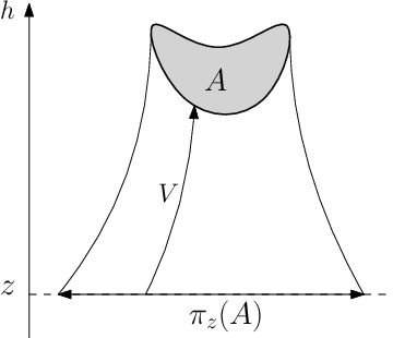
πz​(A):={x∈Xz|Vx∩A≠∅}.\pi_{z}(A):=\left\{x\in X_{z}|V_{x}\cap A\neq\emptyset\right\}. (6)
Refer to caption
Figure 4: Projection of AA on XzX_{z}.

The definition of this projection along the vertical flow is illustrated in Figure 4. The following Lemma shows that the projection of a disk on a horosphere is almost a disk, It will be used in further subsequent sections.

Lemma 1.8.

Let XX be a Gromov hyperbolic, Busemann, proper, geodesically complete metric space. Let z0∈ℝz_{0}\in\mathbb{R} and p∈Xz0p\in X_{z_{0}}. Then for M≥288​δM\geq 288\delta we have that for all z≤z0z\leq z_{0} and for all pz∈πz​({p})p_{z}\in\pi_{z}(\{p\})

D2​(z0−z)−M​(pz)⊂πz​(DM​(p))⊂D2​(z0−z)+M​(pz).\displaystyle D_{2(z_{0}-z)-M}\big(p_{z}\big)\subset\pi_{z}\big(D_{M}(p)\big)\subset D_{2(z_{0}-z)+M}\big(p_{z}\big).
Refer to caption
Figure 5: Proof of Lemma 1.8
Proof.

This Lemma is a corollary of Lemma 1.3 and is illustrated in Figure 5. Let M=288​δM=288\delta be the constant involved in Lemma 1.3.
Let us prove the first inclusion. Let x∈D2​(z0−z)−M​(pz)x\in D_{2(z_{0}-z)-M}\big(p_{z}\big), then d⁡(x,pz)≤2​(z0−z)−Md(x,p_{z})\leq 2(z_{0}-z)-M. Let us denote VxV_{x} a vertical geodesic containing xx and VpV_{p} a vertical geodesic containing pp and pzp_{z}. We apply Lemma 1.3 with t1=t2=zt_{1}=t_{2}=z, V1=VxV_{1}=V_{x} and V2=VpV_{2}=V_{p}, then D=d⁡(x,pz)2D=\frac{d(x,p_{z})}{2}. Moreover

z+D=z+d⁡(x,pz)2≤z+(z0−z)−M2≤z0.\displaystyle z+D=z+\frac{d(x,p_{z})}{2}\leq z+(z_{0}-z)-\frac{M}{2}\leq z_{0}.

Therefore, by the Busemann convexity of XX, the distance between vertical geodesic ray is convex and bounded, hence decreasing. Therefore

d⁡(Vx​(z0),p)\displaystyle d(V_{x}(z_{0}),p) =d⁡(Vx​(z0),Vp​(z0))≤d⁡(Vx​(z+D),Vp​(z+D)),\displaystyle=d(V_{x}(z_{0}),V_{p}(z_{0}))\leq d\big(V_{x}(z+D),V_{p}(z+D)\big),
≤M, by Lemma 1.3 used with ​t=0,\displaystyle\leq M\quad,\text{ by Lemma \ref{LemmaBackward} used with }t=0,

which means that x∈πz​(DM​(p))x\in\pi_{z}\big(D_{M}(p)\big).
Let us now prove the second inclusion, which is

πz​(DM​(p))⊂D2​(z0−z)+M​(pz).\pi_{z}\big(D_{M}(p)\big)\subset D_{2(z_{0}-z)+M}\big(p_{z}\big). (7)

Let x∈πz​(DM​(p))x\in\pi_{z}\big(D_{M}(p)\big), then d⁡(Vx​(z0),Vp​(z0))≤Md(V_{x}(z_{0}),V_{p}(z_{0}))\leq M. Therefore by the triangle inequality

d⁡(x,pz)\displaystyle d(x,p_{z}) =d⁡(Vx​(z),Vp​(z))≤d⁡(Vx​(z),Vx​(z0))+d⁡(Vx​(z0),Vp​(z0))+d⁡(Vp​(z0),Vp​(z)),\displaystyle=d\big(V_{x}(z),V_{p}(z)\big)\leq d\big(V_{x}(z),V_{x}(z_{0})\big)+d\big(V_{x}(z_{0}),V_{p}(z_{0})\big)+d\big(V_{p}(z_{0}),V_{p}(z)\big),
≤(z0−z)+M+(z0−z)=2​(z0−z)+M.\displaystyle\leq(z_{0}-z)+M+(z_{0}-z)=2(z_{0}-z)+M.

Hence x∈D2​(z0−z)+M​(pz)x\in D_{2(z_{0}-z)+M}(p_{z}). ∎

Notations 1.6 can be extended to horospherical products.

Notation 1.9.

Let XX and YY be two proper, hyperbolic, geodesically complete, Busemann spaces. Then:

  1. 1.

    We denote the rr-neighbourhood of UU, for all U⊂X⋈YU\subset X\bowtie Y and for all r≥0r\geq 0, by

    𝒩r​(U):={p∈X⋈Y∣d⋈​(p,U)≤r}.\mathcal{N}_{r}(U):=\{p\in X\bowtie Y\mid d_{\bowtie}(p,U)\leq r\}. (8)
  2. 2.

    The difference of height between two points a,b∈X⋈Ya,b\in X\bowtie Y is still denoted by Δ​h​(a,b):=|h⁡(a)−h⁡(b)|\Delta h\big(a,b\big):=\big|h(a)-h(b)\big|.

  3. 3.

    We still denote, for all z∈ℝz\in\mathbb{R} and A⊂X⋈YA\subset X\bowtie Y, by Az:=A∩h−1​(z)A_{z}:=A\cap h^{-1}(z) the "slice" of AA at the height zz.

  4. 4.

    We still denote, for all r≥0r\geq 0 and p∈X⋈Yp\in X\bowtie Y, by

    Dr​(p):={x∈X∣h⁡(p)=h⁡(x)​ and ​d⋈​(p,x)≤r}=B⁡(p,r)∩(X⋈Y)h⁡(p),\displaystyle D_{r}(p):=\{x\in X\mid h(p)=h(x)\text{ and }d_{\bowtie}(p,x)\leq r\}=B(p,r)\cap(X\bowtie Y)_{h(p)},

    the ball of radius rr in the height level set containing pp.

We recall other useful results of [Fer20] that we will use later. First the fact that the height function is Lipschitz.

Lemma 1.10 (Lemma 3.6 of [Fer20]).

Let NN be an admissible norm, and let d⋈d_{\bowtie} the distance on X⋈YX\bowtie Y induced by NN. Then the height function is 11-Lipschitz with respect to the distance d⋈d_{\bowtie}, i.e.,

∀p,q∈X⋈Y,d⋈​(p,q)≥Δ​h​(p,q).\forall p,q\in X\bowtie Y,\quad d_{\bowtie}(p,q)\geq\Delta h(p,q). (9)

Here is a description of the distance in Horospherical products.

Theorem 1.11 (Corollary 4.13 of [Fer20]).

For all p,q∈X⋈Yp,q\in X\bowtie Y

|d⋈(p,q)−(dY(pY,qY)+dX(pX,qX)−Δh(p,q))|⪯⋈1.\displaystyle\left|d_{\bowtie}(p,q)-\left(d_{Y}\left(p^{Y},q^{Y}\right)+d_{X}\left(p^{X},q^{X}\right)-\Delta h(p,q)\right)\right|\preceq_{\bowtie}1.

Here is one central result of [BH99], let us denote by l⁡(c)l(c) the length of a path cc.

Proposition 1.12 (Proposition 1.61.6, p400 of [BH99]).

Let XX be a δ\delta-hyperbolic geodesic space. Let cc be a continuous path in X. If [p,q][p,q] is a geodesic segment connecting the endpoints of cc, then for every x∈[p,q]x\in[p,q]:

d⁡(x,im⁡(c))≤δ|log2⁡l⁡(c)|+1.d(x,\mathrm{im}(c))\leq\delta|\log_{2}l(c)|+1.

We also provide two more definitions that will be used in future sections. First a projection on level-sets of the height function.

Definition 1.13.

Let z0,z∈ℝz_{0},z\in\mathbb{R} and let U⊂(X⋈Y)z0U\subset(X\bowtie Y)_{z_{0}}. Then we define the projection of U on (X⋈Y)z(X\bowtie Y)_{z} by

πz⋈​(U):={p∈(X⋈Y)z∣∃V​ a vertical geodesic such that ​p∈V​ and ​V∩U≠∅}.\displaystyle\pi_{z}^{\bowtie}(U):=\Big\{p\in(X\bowtie Y)_{z}\mid\exists V\text{ a vertical geodesic such that }p\in V\text{ and }V\cap U\neq\emptyset\Big\}.

Then we define XX-horospheres and YY-horospheres as horospheres of hyperbolic spaces embedded in X⋈YX\bowtie Y, illustrated in Figure 6.

Refer to caption
Figure 6: XX-Horosphere in X⋈YX\bowtie Y.
Definition 1.14.

The set H⊂X⋈YH\subset X\bowtie Y is called

  1. 1.

    an XX-horosphere if there exists y∈Yy\in Y such that H=X⋈{y}=X−h⁡(y)×{y}H=X\bowtie\{y\}=X_{-h(y)}\times\{y\},

  2. 2.

    a YY-horosphere if there exists x∈Xx\in X such that H={x}⋈Y={x}×Y−h⁡(x)H=\{x\}\bowtie Y=\{x\}\times Y_{-h(x)}.

From now on, we will work in a horospherical product X⋈YX\bowtie Y of two proper, geodesically complete, δ\delta-hyperbolic and Busemann spaces.

2 Metric aspects and metric tools in horospherical products

Throughout this section we fix two constants k≥1k\geq 1 and c≥0c\geq 0. We recall the notions of quasi-isometry and quasi-geodesic.

Definition 2.1.

((k,c)(k,c)-quasi-isometry)
Let (E,dE)(E,d_{E}) and (F,dF)(F,d_{F}) be two metric spaces. A map Φ:E→F\Phi:E\to F is called a (k,c)(k,c)-quasi-isometry if and only if:

  1. 1.

    For all x,x′∈Ex,x^{\prime}\in E, k−1​dE​(x,x′)−c≤dF​(Φ⁡(x),Φ⁡(x′))≤k​dE​(x,x′)+ck^{-1}d_{E}(x,x^{\prime})-c\leq d_{F}\left(\Phi(x),\Phi(x^{\prime})\right)\leq kd_{E}(x,x^{\prime})+c.

  2. 2.

    For all y∈Fy\in F, there exists x∈Ex\in E such that d⁡(Φ⁡(x),y)≤cd(\Phi(x),y)\leq c.

A map satisfying Condition 11 is called a quasi-isometric embedding of EE.

Definition 2.2.

((k,c)(k,c)-quasigeodesic)
Let EE be a metric space. A (k,c)(k,c)-quasigeodesic segment, respectively ray, line, of EE is a (k,c)(k,c)-quasi-isometric embedding of a segment, respectively [0;+∞)[0;+\infty), ℝ\mathbb{R}, into EE.

In Lemma 2.12.1 of [GS19], Gouëzel and Shchur prove that any (k,c)(k,c)-quasigeodesic segment is included in the 2​c2c-neighbourhood of a continuous (k,4​c)(k,4c)-quasigeodesic segment sharing the same endpoints. Therefore, without loss of generality, we may consider that all quasi-geodesic segments are continuous.

This section gathers several geometric results on horospherical products, including the generalisation in our context of Lemmas 4.6, 3.1 and the coarse differentiation previously obtained by Eskin, Fisher and Whyte in [EFW12]. Proposition 2.6, Corollary 2.7 and Proposition 2.11 of this section will be especially useful in the following proofs.

At first, a reader who is more interested in the rigidity result on horospherical product can take these propositions for granted and jump to the next sections.

When A≍eBA\asymp_{e}B, and e=(X⋈Y,d)e=(X\bowtie Y,d) is a horospherical product, we shall write A≍⋈BA\asymp_{\bowtie}B as a short-cut, and similarly ⪯⋈\preceq_{\bowtie}, ⪰⋈\succeq_{\bowtie} and M⁡(⋈)M(\bowtie) for a constant depending only on the metric horospherical product (X⋈Y,d⋈)(X\bowtie Y,d_{\bowtie}).

2.1 ε\varepsilon-monotonicity

We introduce ε\varepsilon-monotone quasigeodesics, which happen to remain close to vertical geodesics. This fact plays a key role in our argument and will be proved later.

Definition 2.3.

(ε\varepsilon-monotone quasigeodesic)
Let ε≥0\varepsilon\geq 0 and let α:[0,R]→X⋈Y\alpha:[0,R]\to X\bowtie Y be a quasigeodesic segment. Then α\alpha is called ε\varepsilon-monotone if and only if

∀t1,t2∈[0,R],(h⁡(α⁡(t1))=h⁡(α⁡(t2)))⇒(|t1−t2|≤ε​R).\forall t_{1},t_{2}\in[0,R],\ \ \Big(h\big(\alpha(t_{1})\big)=h\big(\alpha(t_{2})\big)\Big)\Rightarrow\Big(\big|t_{1}-t_{2}\big|\leq\varepsilon R\Big). (10)

Since α\alpha is assumed to be continuous, a 00-monotone quasigeodesic has monotone height, h∘αh\circ\alpha is either decreasing or increasing. We first show that in X⋈YX\bowtie Y, the projections on XX and YY of an ε\varepsilon-monotone quasigeodesic are also quasigeodesics.

Theorem 2.4.

Let ε>0\varepsilon>0, R>1εR>\frac{1}{\varepsilon}, and α=(αX,αY):[0,R]→X⋈Y\alpha=\left(\alpha^{X},\alpha^{Y}\right):[0,R]\to X\bowtie Y be an ε\varepsilon-monotone (k,c)(k,c)-quasigeodesic segment. Then there exists a constant M⁡(⋈,k,c)M(\bowtie,k,c) (depending only on ⋈\bowtie, kk and cc) such that αX\alpha^{X} and αY\alpha^{Y} are (4​k,M​ε​R)(4k,M\varepsilon R)-quasigeodesics.

A portion of the proof of Theorem 2.4 is illustrated in figure 7.

Refer to caption
Figure 7: Proof of Theorem 2.4.
Proof.

We know that ∀p1=(p1X,p1Y)\forall p_{1}=\left(p_{1}^{X},p_{1}^{Y}\right), p2=(p2X,p2Y)∈X⋈Yp_{2}=\left(p_{2}^{X},p_{2}^{Y}\right)\in X\bowtie Y we have (this is the admissible assumption we made on the norm underneath the distance d⋈d_{\bowtie})

d⋈​(p1,p2)≥dX​(p1X,p2X)+dY​(p1Y,p2Y)2.d_{\bowtie}(p_{1},p_{2})\geq\frac{d_{X}\left(p_{1}^{X},p_{2}^{X}\right)+d_{Y}\left(p_{1}^{Y},p_{2}^{Y}\right)}{2}. (11)

Therefore we have that αX\alpha^{X} satisfies the upper-bound assumption of quasigeodesics

∀s1,s2∈[0,R],dX​(αX​(s1),αX​(s2))≤2​d⋈​(α⁡(s1),α⁡(s2))≤2​k​|s1−s2|+2​c.\displaystyle\forall s_{1},s_{2}\in[0,R],\ d_{X}\left(\alpha^{X}(s_{1}),\alpha^{X}(s_{2})\right)\leq 2d_{\bowtie}\big(\alpha(s_{1}),\alpha(s_{2})\big)\leq 2k|s_{1}-s_{2}|+2c.

We want to find an appropriate c′≥cc^{\prime}\geq c such that αX\alpha^{X} satisfies the lower-bound condition of a (4​k,c′)(4k,c^{\prime})-quasigeodesic. Let c′≥cc^{\prime}\geq c and let us assume that αX\alpha^{X} does not satisfy the lower-bound condition of a (4​k,c′)(4k,c^{\prime})-quasigeodesic, we will show that this provides us with an upper-bound on c′c^{\prime}. Indeed, consider s1,s2∈[0,R]s_{1},s_{2}\in[0,R] such that

0≤dX​(αX​(s1),αX​(s2))\displaystyle 0\leq d_{X}\left(\alpha^{X}(s_{1}),\alpha^{X}(s_{2})\right) ≤14​k​|s1−s2|−c′.\displaystyle\leq\frac{1}{4k}|s_{1}-s_{2}|-c^{\prime}. (12)

Therefore by the Lipschitz property of hh

Δ​h​(αX​(s1),αX​(s2))\displaystyle\Delta h\left(\alpha^{X}(s_{1}),\alpha^{X}(s_{2})\right) ≤dX​(αX​(s1),αX​(s2))≤14​k​|s1−s2|−c′,\displaystyle\leq d_{X}\left(\alpha^{X}(s_{1}),\alpha^{X}(s_{2})\right)\leq\frac{1}{4k}|s_{1}-s_{2}|-c^{\prime},
≤14​d⋈​(α⁡(s1),α⁡(s2))+c4−c′, since ​α​ is a ​(k,c)​- quasigeodesic.\displaystyle\leq\frac{1}{4}d_{\bowtie}(\alpha(s_{1}),\alpha(s_{2})\big)+\frac{c}{4}-c^{\prime},\quad\text{ since }\alpha\text{ is a }(k,c)\text{- quasigeodesic}. (13)

Theorem 1.11 gives us the existence of a constant M⁡(⋈)M(\bowtie) depending only on XX, YY and the underlying norm of d⋈d_{\bowtie} such that

dY​(αY​(s1),αY​(s2))\displaystyle d_{Y}\left(\alpha^{Y}(s_{1}),\alpha^{Y}(s_{2})\right) (14)
≥\displaystyle\geq d⋈​(α⁡(s1),α⁡(s2))−dX​(αX​(s1),αX​(s2))+Δ​h​(α⁡(s1),α⁡(s2))−M,\displaystyle d_{\bowtie}\big(\alpha(s_{1}),\alpha(s_{2})\big)-d_{X}\left(\alpha^{X}(s_{1}),\alpha^{X}(s_{2})\right)+\Delta h\big(\alpha(s_{1}),\alpha(s_{2})\big)-M,
≥\displaystyle\geq d⋈​(α⁡(s1),α⁡(s2))−dX​(αX​(s1),αX​(s2))−M,\displaystyle d_{\bowtie}\big(\alpha(s_{1}),\alpha(s_{2})\big)-d_{X}\left(\alpha^{X}(s_{1}),\alpha^{X}(s_{2})\right)-M,
≥\displaystyle\geq d⋈​(α⁡(s1),α⁡(s2))−14​k​|s1−s2|+c′−M,by assumption (12),\displaystyle d_{\bowtie}\big(\alpha(s_{1}),\alpha(s_{2})\big)-\frac{1}{4k}|s_{1}-s_{2}|+c^{\prime}-M,\quad\text{by assumption (\ref{InesAssumptionOns1s23}),}
≥\displaystyle\geq d⋈​(α⁡(s1),α⁡(s2))−14​d⋈​(α⁡(s1),α⁡(s2))−c4​k+c′−M,since ​α​ is a ​(k,c)​-quasigeodesic,\displaystyle d_{\bowtie}\big(\alpha(s_{1}),\alpha(s_{2})\big)-\frac{1}{4}d_{\bowtie}\big(\alpha(s_{1}),\alpha(s_{2})\big)-\frac{c}{4k}+c^{\prime}-M,\quad\text{since }\alpha\text{ is a }(k,c)\text{-quasigeodesic,}
≥\displaystyle\geq 12​d⋈​(α⁡(s1),α⁡(s2))−c4+c′−M,since ​k≥1.\displaystyle\frac{1}{2}d_{\bowtie}\big(\alpha(s_{1}),\alpha(s_{2})\big)-\frac{c}{4}+c^{\prime}-M,\quad\text{since }k\geq 1. (15)

Without loss of generality, we may assume that max⁡(h⁡(αY​(s1)),h⁡(αY​(s2)))=h⁡(αY​(s2))\max\Big(h\left(\alpha^{Y}(s_{1})\right),h\left(\alpha^{Y}(s_{2})\right)\Big)=h\left(\alpha^{Y}(s_{2})\right). Applying Lemma 1.5 on the geodesic [αY​(s1),αY​(s2)]\left[\alpha^{Y}(s_{1}),\alpha^{Y}(s_{2})\right] of YY gives us

h+​([αY​(s1),αY​(s2)])≥h⁡(αY​(s2))+12​(dY​(αY​(s1),αY​(s2))−Δ​h​(αY​(s1),αY​(s2)))−M⁡(⋈).\displaystyle h^{+}\left(\left[\alpha^{Y}(s_{1}),\alpha^{Y}(s_{2})\right]\right)\geq h\left(\alpha^{Y}(s_{2})\right)+\frac{1}{2}\Big(d_{Y}\left(\alpha^{Y}(s_{1}),\alpha^{Y}(s_{2})\right)-\Delta h\left(\alpha^{Y}(s_{1}),\alpha^{Y}(s_{2})\right)\Big)-M(\bowtie).

However αY\alpha^{Y} is a continuous path between αY​(s1)\alpha^{Y}(s_{1}) and αY​(s2)\alpha^{Y}(s_{2}), then by Proposition 1.12, there exists s0∈[s1,s2]s_{0}\in[s_{1},s_{2}] such that

h⁡(αY​(s0))≥\displaystyle h\left(\alpha^{Y}(s_{0})\right)\geq h⁡(αY​(s2))+12​(dY​(αY​(s1),αY​(s2))−Δ​h​(αY​(s1),αY​(s2)))\displaystyle h\left(\alpha^{Y}(s_{2})\right)+\frac{1}{2}\Big(d_{Y}\left(\alpha^{Y}(s_{1}),\alpha^{Y}(s_{2})\right)-\Delta h\left(\alpha^{Y}(s_{1}),\alpha^{Y}(s_{2})\right)\Big)
−δ​log2⁡(dY​(αY​(s1),αY​(s2)))−M⁡(⋈).\displaystyle-\delta\log_{2}\big(d_{Y}\left(\alpha^{Y}(s_{1}),\alpha^{Y}(s_{2})\right)\big)-M(\bowtie).

Therefore by inequalities (13) and (15)

h⁡(αY​(s0))≥\displaystyle h\left(\alpha^{Y}(s_{0})\right)\geq h⁡(αY​(s2))+14​d⋈​(α⁡(s1),α⁡(s2))−18​d⋈​(α⁡(s1),α⁡(s2))−c4+c′−c8+12​c′\displaystyle h\left(\alpha^{Y}(s_{2})\right)+\frac{1}{4}d_{\bowtie}\left(\alpha(s_{1}),\alpha(s_{2})\right)-\frac{1}{8}d_{\bowtie}\left(\alpha(s_{1}),\alpha(s_{2})\right)-\frac{c}{4}+c^{\prime}-\frac{c}{8}+\frac{1}{2}c^{\prime}
−δ​log2⁡(dY​(αY​(s1),αY​(s2)))−M⁡(⋈)2,\displaystyle-\delta\log_{2}\big(d_{Y}\left(\alpha^{Y}(s_{1}),\alpha^{Y}(s_{2})\right)\big)-\frac{M(\bowtie)}{2},
≥\displaystyle\geq h⁡(αY​(s2))+18​d⋈​(α⁡(s1),α⁡(s2))−δ​log2⁡(dY​(αY​(s1),αY​(s2)))+32​c′−M⁡(⋈,c).\displaystyle h\left(\alpha^{Y}(s_{2})\right)+\frac{1}{8}d_{\bowtie}\left(\alpha(s_{1}),\alpha(s_{2})\right)-\delta\log_{2}\big(d_{Y}\left(\alpha^{Y}(s_{1}),\alpha^{Y}(s_{2})\right)\big)+\frac{3}{2}c^{\prime}-M(\bowtie,c).

However 2​d⋈≥dX+dY≥dY2d_{\bowtie}\geq d_{X}+d_{Y}\geq d_{Y}, hence

h⁡(αY​(s0))≥h⁡(αY​(s2))+18​d⋈​(α⁡(s1),α⁡(s2))−δ​log2⁡(d⋈​(α⁡(s1),α⁡(s2)))+32​c′−M⁡(⋈,c).\displaystyle h\left(\alpha^{Y}(s_{0})\right)\geq h\left(\alpha^{Y}(s_{2})\right)+\frac{1}{8}d_{\bowtie}\left(\alpha(s_{1}),\alpha(s_{2})\right)-\delta\log_{2}\big(d_{\bowtie}\left(\alpha(s_{1}),\alpha(s_{2})\right)\big)+\frac{3}{2}c^{\prime}-M(\bowtie,c). (16)

Furthermore, there exists r0∈ℝr_{0}\in\mathbb{R} depending only on δ\delta such that ∀r≥r0\forall r\geq r_{0}, 18​r−δ​log2⁡(r)>110​r\frac{1}{8}r-\delta\log_{2}(r)>\frac{1}{10}r holds. Therefore, one of the two following statements holds:

  1. (a)

    d⋈​(α⁡(s1),α⁡(s2))<r0d_{\bowtie}\left(\alpha(s_{1}),\alpha(s_{2})\right)<r_{0}.

  2. (b)

    18​d⋈​(α⁡(s1),α⁡(s2))−δ​log2⁡(d⋈​(α⁡(s1),α⁡(s2)))≥110​d⋈​(α⁡(s1),α⁡(s2))\frac{1}{8}d_{\bowtie}\left(\alpha(s_{1}),\alpha(s_{2})\right)-\delta\log_{2}\left(d_{\bowtie}\left(\alpha(s_{1}),\alpha(s_{2})\right)\right)\geq\frac{1}{10}d_{\bowtie}\left(\alpha(s_{1}),\alpha(s_{2})\right).

We will deal with the first case (a)(a) at the end of the proof. Let us assume that d⋈​(α⁡(s1),α⁡(s2))≥r0d_{\bowtie}\left(\alpha(s_{1}),\alpha(s_{2})\right)\geq r_{0} hence (b)(b), then by inequality (16)

h⁡(αY​(s0))≥h⁡(αY​(s2))+110​d⋈​(α⁡(s1),α⁡(s2))+32​c′−M⁡(⋈,c).\displaystyle h\left(\alpha^{Y}(s_{0})\right)\geq h\left(\alpha^{Y}(s_{2})\right)+\frac{1}{10}d_{\bowtie}\left(\alpha(s_{1}),\alpha(s_{2})\right)+\frac{3}{2}c^{\prime}-M(\bowtie,c). (17)

Then either d⋈​(α⁡(s1),α⁡(s2))≤M⁡(⋈,c)d_{\bowtie}\big(\alpha(s_{1}),\alpha(s_{2})\big)\leq M(\bowtie,c) (up to multiplying by 1010 the constant MM), or h⁡(αY​(s0))≥h⁡(αY​(s2))h(\alpha^{Y}(s_{0}))\geq h(\alpha^{Y}(s_{2})). In the case d⋈​(α⁡(s1),α⁡(s2))≤M⁡(⋈,c)d_{\bowtie}\big(\alpha(s_{1}),\alpha(s_{2})\big)\leq M(\bowtie,c), then |s1−s2|⪯k,c,⋈1|s_{1}-s_{2}|\preceq_{k,c,\bowtie}1 since α\alpha is a quasigeodesic, and therefore c′⪯k,c,⋈1c^{\prime}\preceq_{k,c,\bowtie}1 following assumption (12). In the other case we have h⁡(αY​(s0))≥h⁡(αY​(s2))h(\alpha^{Y}(s_{0}))\geq h(\alpha^{Y}(s_{2})), therefore there exists s1′∈[s1,s0]s_{1}^{\prime}\in[s_{1},s_{0}] such that h⁡(αY​(s1′))=h⁡(αY​(s2))h\left(\alpha^{Y}(s_{1}^{\prime})\right)=h\left(\alpha^{Y}(s_{2})\right), since α\alpha is continuous. Hence

d⋈​(α⁡(s1′),α⁡(s2))≥\displaystyle d_{\bowtie}\big(\alpha(s_{1}^{\prime}),\alpha(s_{2})\big)\geq 1k​|s1′−s2|−c≥1k​(|s1′−s0|+|s0−s2|)−M⁡(c),since ​α​ is a quasigeodesic,\displaystyle\frac{1}{k}|s_{1}^{\prime}-s_{2}|-c\geq\frac{1}{k}\big(|s_{1}^{\prime}-s_{0}|+|s_{0}-s_{2}|\big)-M(c),\quad\text{since }\alpha\text{ is a quasigeodesic},
≥\displaystyle\geq 1k2​(d⋈​(α⁡(s1′),α⁡(s0))+d⋈​(α⁡(s0),α⁡(s2)))−M⁡(k,c),since ​α​ is a quasigeodesic,\displaystyle\frac{1}{k^{2}}\Big(d_{\bowtie}\big(\alpha(s_{1}^{\prime}),\alpha(s_{0})\big)+d_{\bowtie}\big(\alpha(s_{0}),\alpha(s_{2})\big)\Big)-M(k,c),\quad\text{since }\alpha\text{ is a quasigeodesic},
≥\displaystyle\geq 1k2​(Δ​h​(α⁡(s1′),α⁡(s0))+Δ​h​(α⁡(s0),α⁡(s2)))−M⁡(k,c),by Lemma 1.10,\displaystyle\frac{1}{k^{2}}\Big(\Delta h\big(\alpha(s_{1}^{\prime}),\alpha(s_{0})\big)+\Delta h\big(\alpha(s_{0}),\alpha(s_{2})\big)\Big)-M(k,c),\quad\text{by Lemma \ref{LemDistBigHaut}},
≥\displaystyle\geq 2k2​Δ​h​(α⁡(s0),α⁡(s2))−M⁡(k,c),since ​h​(α⁡(s1′))=h⁡(α⁡(s2)),\displaystyle\frac{2}{k^{2}}\Delta h\big(\alpha(s_{0}),\alpha(s_{2})\big)-M(k,c),\quad\text{since }h\big(\alpha(s_{1}^{\prime})\big)=h\big(\alpha(s_{2})\big),
≥\displaystyle\geq 15​k2d⋈(α(s1),α(s2))+3k2c′−M(k,c,⋈),by (17).\displaystyle\frac{1}{5k^{2}}d_{\bowtie}\left(\alpha(s_{1}),\alpha(s_{2})\right)+\frac{3}{k^{2}}c^{\prime}-M(k,c,\bowtie),\quad\text{by (\ref{Ineq3LemmeMonotVertCloseGeod})}. (18)

Moreover assumption (12) implies |s1−s2|≥4​k​c′|s_{1}-s_{2}|\geq 4kc^{\prime}. Then

d⋈​(α⁡(s1),α⁡(s2))\displaystyle d_{\bowtie}\big(\alpha(s_{1}),\alpha(s_{2})\big) ≥1k​|s1−s2|−c≥4​c′−c.\displaystyle\geq\frac{1}{k}|s_{1}-s_{2}|-c\geq 4c^{\prime}-c.

Combined with inequality (18) it gives us

d⋈(α(s1′),α(s2))≥195​k2c′−M(k,c,⋈).\displaystyle d_{\bowtie}\big(\alpha(s_{1}^{\prime}),\alpha(s_{2})\big)\geq\frac{19}{5k^{2}}c^{\prime}-M(k,c,\bowtie).

Since α\alpha is ε\varepsilon-monotone and because h⁡(αY​(s1′))=h⁡(αY​(s2))h\left(\alpha^{Y}(s_{1}^{\prime})\right)=h\left(\alpha^{Y}(s_{2})\right), we have

ε​R≥\displaystyle\varepsilon R\geq |s1′−s2|≥d⋈(α(s1′),α(s2))≥195​k2c′−M(k,c,⋈).\displaystyle|s_{1}^{\prime}-s_{2}|\geq d_{\bowtie}\big(\alpha(s_{1}^{\prime}),\alpha(s_{2})\big)\geq\frac{19}{5k^{2}}c^{\prime}-M(k,c,\bowtie).

Hence

c′≤M(k)εR+M(k,c,⋈).\displaystyle c^{\prime}\leq M(k)\varepsilon R+M(k,c,\bowtie).

We proved that if αX\alpha^{X} does not satisfy the lower bound inequality for being a (4​k,c′)(4k,c^{\prime})-quasigeodesic, then c′≤M(k)εR+M(k,c,⋈)c^{\prime}\leq M(k)\varepsilon R+M(k,c,\bowtie). Thus, when ε​R≥1\varepsilon R\geq 1, there exists a constant M(k,c,⋈)M(k,c,\bowtie) such that αX\alpha^{X} is a (4​k,M​ε​R)(4k,M\varepsilon R)-quasigeodesic in both subcases of case (b)(b) under consideration. Similarly we show that αY\alpha^{Y} is a (4​k,M​ε​R)(4k,M\varepsilon R)-quasigeodesic segment of YY.

For case (a)(a), let us assume that each couple of times (s1,s2)∈[0,R]2(s_{1},s_{2})\in[0,R]^{2} that contradicts the lower-bound hypothesis of a (4​k,M​ε​R)(4k,M\varepsilon R)-quasigeodesic verifies that d⋈​(α⁡(s1),α⁡(s2))<r0d_{\bowtie}(\alpha(s_{1}),\alpha(s_{2}))<r_{0}. Then α\alpha is a (4​k,r0)(4k,r_{0})-quasigeodesic, with r0r_{0} depending only on δ\delta. Therefore α\alpha is in both cases a (4​k,M​ε​R)(4k,M\varepsilon R)-quasigeodesic, with MM depending only on k,ck,c and X⋈YX\bowtie Y. ∎

In the sequel we denote by dHffd_{\mathrm{Hff}} the Hausdorff distance induced by d⋈d_{\bowtie}. In the the proof of Lemma 2.6 we use a quantitative version of the quasigeodesic rigidity in a Gromov hyperbolic space, provided by the main theorem of [GS19].

Theorem 2.5.

([GS19])
Consider a (k,C)(k,C)-quasigeodesic segment α\alpha in a δ\delta-hyperbolic space XX, and γ\gamma a geodesic segment between its endpoints. Then the Hausdorff distance dHff​(α,γ)d_{\mathrm{Hff}}(\alpha,\gamma) between α\alpha and γ\gamma satisfies

dHff​(α,γ)≤92​k2​(C+δ).\displaystyle d_{\mathrm{Hff}}(\alpha,\gamma)\leq 92k^{2}(C+\delta).

This quantitative version allows us to have a linear control with respect to CC on the Hausdorff distance, which is mandatory in our cases since C≍ε​RC\asymp\varepsilon R. Combining this rigidity with the fact that projections αX\alpha^{X} and αY\alpha^{Y} are also ε\varepsilon-monotone provides us with the existence of vertical geodesic segments close to α\alpha.

Proposition 2.6.

Let ε>0\varepsilon>0, R>1εR>\frac{1}{\varepsilon}, and α:[0,R]→X⋈Y\alpha:[0,R]\to X\bowtie Y be an ε\varepsilon-monotone (k,c)(k,c)-quasigeodesic segment. Then there exists a vertical geodesic segment V:[0,R]→X⋈YV:[0,R]\to X\bowtie Y such that

dHff(im(α),im(V))⪯k,c,δεR.d_{\mathrm{Hff}}\big(\mathrm{im}(\alpha),\mathrm{im}(V)\big)\preceq_{k,c,\delta}\varepsilon R. (19)

This proposition corresponds to Lemma 4.6 in [EFW12].

Figure 8 is an illustration of the proof.

Refer to caption
Figure 8: Proof of Proposition 2.6
Proof.

By Theorem 2.4, αX\alpha^{X} is a (4​k,M​ε​R)(4k,M\varepsilon R)-quasi-geodesic in XX which is δ\delta-hyperbolic, hence by Theorem 2.5 there exists a geodesic γX\gamma^{X} with the same endpoints as αX\alpha^{X} such that

dHff(im(αX),im(γX))⪯k,c,δεR.\displaystyle d_{\mathrm{Hff}}\Big(\mathrm{im}\left(\alpha^{X}\right),\mathrm{im}\left(\gamma^{X}\right)\Big)\preceq_{k,c,\delta}\varepsilon R.

Let us denote x1:=αX​(0)x_{1}:=\alpha^{X}(0) and x2:=αX​(R)x_{2}:=\alpha^{X}(R). The quasigeodesic αX\alpha^{X} is also ε\varepsilon-monotone. Furthermore Proposition 2.22.2 page 19 of [CDP90] gives us that γX\gamma^{X}, which links x1x_{1} to x2x_{2}, is included in the 24​δ24\delta-neighbourhood of two vertical geodesic rays V1V_{1} and V2V_{2} such that V1​(0)=x1V_{1}(0)=x_{1} and V2​(0)=x2V_{2}(0)=x_{2}. Let us denote τ:=h+​(γX)\tau:=h^{+}\left(\gamma^{X}\right), and let us recall that ∀t1,t2∈ℝ+\forall t_{1},t_{2}\in\mathbb{R}^{+} and for i∈{1,2}i\in\{1,2\} we have Δ​h​(Vi​(t1),Vi​(t2))=|t1−t2|\Delta h\left(V_{i}(t_{1}),V_{i}(t_{2})\right)=|t_{1}-t_{2}|. Let us also denote by slight abuse γX:=im⁡(γX)\gamma^{X}:=\mathrm{im}\left(\gamma^{X}\right), αX:=im⁡(αX)\alpha^{X}:=\mathrm{im}\left(\alpha^{X}\right), V1:=im⁡(V1|[0,τ−h⁡(x1)])V_{1}:=\mathrm{im}\left(V_{1|[0,\tau-h(x_{1})]}\right) and V2:=im⁡(V2|[0,τ−h⁡(x2)])V_{2}:=\mathrm{im}\left(V_{2|[0,\tau-h(x_{2})]}\right). Since τ=h+​(γX)=h+​(V1)=h+​(V2)\tau=h^{+}\left(\gamma^{X}\right)=h^{+}\left(V_{1}\right)=h^{+}\left(V_{2}\right) we have

dHff(γX,V1∪V2)⪯δ1.\displaystyle d_{\mathrm{Hff}}\Big(\gamma^{X},V_{1}\cup V_{2}\Big)\preceq_{\delta}1.

Hence by the triangle inequality

dHff(αX,V1∪V2)⪯k,c,δεR.\displaystyle d_{\mathrm{Hff}}\Big(\alpha^{X},V_{1}\cup V_{2}\Big)\preceq_{k,c,\delta}\varepsilon R. (20)

Without loss of generality we can assume that h⁡(x1)≤h⁡(x2)h(x_{1})\leq h(x_{2}). Furthermore γX\gamma^{X} is continuous, therefore there exists a point of γX\gamma^{X} close to both vertical geodesics (less than 24​δ24\delta apart). Furthermore XX is Busemann convex, hence the distance between the two vertical geodesics is decreasing. Therefore dX(V1(τ−h(x1)),V2(τ−h(x2)))⪯δ1d_{X}\Big(V_{1}\big(\tau-h(x_{1})\big),V_{2}\big(\tau-h(x_{2})\big)\Big)\preceq_{\delta}1. We will use the ε\varepsilon-monotonicity of αX\alpha^{X} to prove that τ≈h⁡(x2)\tau\approx h(x_{2}). Let us denote by x1′x_{1}^{\prime} a point of αX\alpha^{X} such that h⁡(x1′)=h⁡(x2)h(x_{1}^{\prime})=h(x_{2}) and such that dX(x1′,V1)⪯k,c,δεRd_{X}(x_{1}^{\prime},\mathrm{V_{1}})\preceq_{k,c,\delta}\varepsilon R. Since αX\alpha^{X} is ε\varepsilon-monotone and a (4​k,M​ε​R)(4k,M\varepsilon R)-quasigeodesic we have that dX(x1′,x2)⪯k,cεRd_{X}(x_{1}^{\prime},x_{2})\preceq_{k,c}\varepsilon R, hence using the triangle inequality we have

dX​(V1​(h⁡(x2)−h⁡(x1)),x2)\displaystyle d_{X}\Big(V_{1}\big(h(x_{2})-h(x_{1})\big),x_{2}\Big) ≤dX​(V1​(h⁡(x2)−h⁡(x1)),x1′)+dX​(x1′,x2),\displaystyle\leq d_{X}\Big(V_{1}\big(h(x_{2})-h(x_{1})\big),x_{1}^{\prime}\Big)+d_{X}\big(x_{1}^{\prime},x_{2}\big),
⪯k,c,δεR.\displaystyle\preceq_{k,c,\delta}\varepsilon R. (21)

Let g1∈im⁡(γX)g_{1}\in\mathrm{im}\left(\gamma^{X}\right) be the closest point to x1x_{1} at height h⁡(x2)h(x_{2}). Then we have:

  1. 1.

    dX(g1,V1(h(x2)−h(x1)))⪯δ1d_{X}\Big(g_{1},V_{1}\big(h(x_{2})-h(x_{1})\big)\Big)\preceq_{\delta}1;

  2. 2.

    dX​(g1,x2)≥2​(h+​(γX)−h⁡(x2))d_{X}(g_{1},x_{2})\geq 2\left(h^{+}\left(\gamma^{X}\right)-h(x_{2})\right).

We recall that τ=h+​(γX)\tau=h^{+}\left(\gamma^{X}\right), then dX​(g1,x2)≥2​τ−2​h​(x2)≥0d_{X}(g_{1},x_{2})\geq 2\tau-2h(x_{2})\geq 0, hence

|τ−h⁡(x2)|\displaystyle|\tau-h(x_{2})| ≤12​dX​(g1,x2)≤12​dX​(g1,V1​(h⁡(x2)−h⁡(x1)))+12​dX​(V1​(h⁡(x2)−h⁡(x1)),x2),\displaystyle\leq\frac{1}{2}d_{X}(g_{1},x_{2})\leq\frac{1}{2}d_{X}\Big(g_{1},V_{1}\big(h(x_{2})-h(x_{1})\big)\Big)+\frac{1}{2}d_{X}\Big(V_{1}\big(h(x_{2})-h(x_{1})\big),x_{2}\Big),
⪯k,c,δεR,by definition of g1 and inequality (21).\displaystyle\preceq_{k,c,\delta}\varepsilon R,\quad\text{by definition of }g_{1}\text{ and inequality }(\ref{IneqMonotHoroCloseVertHoro}).

Hence V2|[0,τ−h⁡(x2)]V_{2|[0,\tau-h(x_{2})]} is a vertical geodesic segment of length ⪯k,c,δεR\preceq_{k,c,\delta}\varepsilon R. Furthermore, dX(V1(τ−h(x1)),V2(τ−h(x2)))≤δd_{X}(V_{1}(\tau-h(x_{1})),V_{2}(\tau-h(x_{2})))\leq_{\delta}. Therefore by the triangle inequality, any point of V2|[0,τ−h⁡(x2)]V_{2|[0,\tau-h(x_{2})]} is (up to a multiplicative constant) ε​R\varepsilon R-close to V1​(τ−h⁡(x1))V_{1}(\tau-h(x_{1})). Therefore dHff(V1∪V2,V1)⪯k,c,δεRd_{\mathrm{Hff}}(V_{1}\cup V_{2},V_{1})\preceq_{k,c,\delta}\varepsilon R. Therefore, by the triangle inequality we can improve inequality (20) as follows

dHff​(αX,V1)\displaystyle d_{\mathrm{Hff}}\Big(\alpha^{X},V_{1}\Big) ≤dHff​(αX,V1∪V2)+dHff​(V1∪V2,V1),\displaystyle\leq d_{\mathrm{Hff}}\Big(\alpha^{X},V_{1}\cup V_{2}\Big)+d_{\mathrm{Hff}}\Big(V_{1}\cup V_{2},V_{1}\Big),
⪯k,c,δεR, by inequality (20).\displaystyle\preceq_{k,c,\delta}\varepsilon R,\quad\text{ by inequality (\ref{IneqtwoGeodVertIntoOne})}.

We deduce similarly that αY\alpha^{Y} is included in the M​ε​RM\varepsilon R-neighbourhood of a vertical geodesic segment V2′V_{2}^{\prime}. Therefore, α\alpha is included in the M​ε​RM\varepsilon R-neighbourhood of the vertical geodesic segment (V1,V2′)(V_{1},V_{2}^{\prime}). ∎

As a corollary, we show that the height function along an ε\varepsilon-monotone quasigeodesic is a quasi-isometry embedding of a segment into ℝ\mathbb{R}.

Corollary 2.7.

Let α:[0,R]↦X⋈Y\alpha:[0,R]\mapsto X\bowtie Y be an ε\varepsilon-monotone (k,c)(k,c)-quasigeodesic segment. Then there exists a constant M⁡(k,c,δ)M(k,c,\delta) such that the height function verifies ∀t1,t2∈[0,R]\forall t_{1},t_{2}\in[0,R]

1k​|t1−t2|−M​ε​R≤Δ​h​(α⁡(t1),α⁡(t2))≤k|t1−t2|+M​ε​R.\displaystyle\frac{1}{k}|t_{1}-t_{2}|-M\varepsilon R\leq\Delta h\big(\alpha(t_{1}),\alpha(t_{2})\big)\leq k|t_{1}-t_{2}|+M\varepsilon R. (22)
Proof.

Let t1,t2∈[0,R]t_{1},t_{2}\in[0,R]. The quasigeodesic upper-bound inequality is straightforward since hh is 11-Lipschitz and α\alpha is a (k,c)(k,c)-quasigeodesic.

Δ​h​(α⁡(t1),α⁡(t2))≤d⋈​(α⁡(t1),α⁡(t2))≤k|t1−t2|+c.\displaystyle\Delta h(\alpha(t_{1}),\alpha(t_{2}))\leq d_{\bowtie}(\alpha(t_{1}),\alpha(t_{2}))\leq k|t_{1}-t_{2}|+c.

To achieve the lower-bound inequality we use Proposition 2.6, hence there exists a vertical geodesic segment V:[0,R]→X⋈YV:[0,R]\to X\bowtie Y and a constant M⁡(k,c,δ)M(k,c,\delta) such that

dHff​(im⁡(α),im⁡(V))≤M​ε​R.d_{\mathrm{Hff}}\big(\mathrm{im}(\alpha),\mathrm{im}(V)\big)\leq M\varepsilon R. (23)

For i∈{1,2}i\in\{1,2\}, let si∈[0,R]s_{i}\in[0,R] be such that d⋈​(α⁡(ti),V⁡(si))≤M​ε​Rd_{\bowtie}(\alpha(t_{i}),V(s_{i}))\leq M\varepsilon R. Then by the triangle inequality

Δ​h​(α⁡(t1),α⁡(t2))\displaystyle\Delta h(\alpha(t_{1}),\alpha(t_{2})) ≥Δ​h​(V⁡(s1),V⁡(s2))−2​M​ε​R,\displaystyle\geq\Delta h(V(s_{1}),V(s_{2}))-2M\varepsilon R,
=|s1−s2|−2​M​ε​R,since V is vertical.\displaystyle=|s_{1}-s_{2}|-2M\varepsilon R,\quad\text{since V is vertical}.

However we can achieve the lower-bound inequality on |s1−s2||s_{1}-s_{2}|

|s1−s2|=d⋈​((V⁡(s1),V⁡(s2))CLOSE\displaystyle|s_{1}-s_{2}|=d_{\bowtie}((V(s_{1}),V(s_{2})) ≥d⋈​(α⁡(t1),α⁡(t2))−2​M​ε​R,by the triangle inequality,\displaystyle\geq d_{\bowtie}(\alpha(t_{1}),\alpha(t_{2}))-2M\varepsilon R,\quad\text{by the triangle inequality,}
≥1k​|t1−t2|−c−2​M​ε​R,since ​α​ is a quasigeodesic.\displaystyle\geq\frac{1}{k}|t_{1}-t_{2}|-c-2M\varepsilon R,\quad\text{since }\alpha\text{ is a quasigeodesic}.

Which provides us with

Δ​h​(α⁡(t1),α⁡(t2))\displaystyle\Delta h(\alpha(t_{1}),\alpha(t_{2})) ≥|s1−s2|−2​M​ε​R≥1k​|t1−t2|−5​M​ε​R.\displaystyle\geq|s_{1}-s_{2}|-2M\varepsilon R\geq\frac{1}{k}|t_{1}-t_{2}|-5M\varepsilon R.

∎

2.2 Coarse differentiation of a quasigeodesic segment

The coarse differentiation of a quasigeodesic α\alpha consists in finding a scale r>0r>0 such that a subdivision by pieces of length rr of α\alpha contains almost only ε\varepsilon-monotone components (which are therefore close to vertical geodesic segments).

Proposition 2.9 provides us with the existence of such an appropriate scale .

Lemma 2.8.

Let k≥1k\geq 1, c≥0c\geq 0 and ε>0\varepsilon>0. There exists M(k,c,⋈,ε)M(k,c,\bowtie,\varepsilon) such that for all r≥Mr\geq M, N≥MN\geq M and for all non ε\varepsilon-monotone, (k,c)(k,c)-quasigeodesic segment α:[0,r]→X⋈Y\alpha:[0,r]\to X\bowtie Y we have

∑j=0N−1Δh(α(j​rN),α((j+1)​rN))−Δh(α(0),α(r))⪰k,c⋈εr.\sum\limits_{j=0}^{N-1}\Delta h\left(\alpha\left(\dfrac{jr}{N}\right),\alpha\left(\dfrac{(j+1)r}{N}\right)\right)-\Delta h\big(\alpha(0),\alpha(r)\big)\succeq_{k,c\bowtie}\varepsilon r. (24)

This proposition corresponds to Lemma 4.7 in [EFW12].

Refer to caption
Figure 9: Subdivision of a quasi-geodesic.
Proof.

Since α\alpha is non ε\varepsilon-monotone, there exist t1,t3∈[0,r]t_{1},t_{3}\in[0,r] such that

h⁡(α⁡(t1))=h⁡(α⁡(t3))and|t1−t3|>ε​r.h(\alpha(t_{1}))=h(\alpha(t_{3}))\quad\text{and}\quad|t_{1}-t_{3}|>\varepsilon r. (25)

We can assume without loss of generality that h⁡(α⁡(0))≤h⁡(α⁡(t1))≤h⁡(α⁡(r))h(\alpha(0))\leq h(\alpha(t_{1}))\leq h(\alpha(r)) with t1<t3t_{1}<t_{3}. Since α\alpha is a (k,c)(k,c)-quasigeodesic we have d⋈​(α⁡(t1),α⁡(t3))≥ε​rk−cd_{\bowtie}\big(\alpha(t_{1}),\alpha(t_{3})\big)\geq\dfrac{\varepsilon r}{k}-c. By Corollary 1.11 of the first part of this manuscript, there exists M⁡(⋈)M(\bowtie) such that d⋈≤dX+dY+Md_{\bowtie}\leq d_{X}+d_{Y}+M. Then at least one of the two following inequalities holds:

  1. 1.

    dX(αX(t1),αX(t3))⪰⋈ε2​kr−M(⋈,c)d_{X}\left(\alpha^{X}(t_{1}),\alpha^{X}(t_{3})\right)\succeq_{\bowtie}\frac{\varepsilon}{2k}r-M(\bowtie,c);

  2. 2.

    dY(αY(t1),αY(t3))⪰⋈ε2​kr−M(⋈,c)d_{Y}\left(\alpha^{Y}(t_{1}),\alpha^{Y}(t_{3})\right)\succeq_{\bowtie}\frac{\varepsilon}{2k}r-M(\bowtie,c).

Let us assume that the first inequality is true. By Lemma 1.5 applied to the geodesic segment [αX​(t1),αX​(t3)]\left[\alpha^{X}(t_{1}),\alpha^{X}(t_{3})\right] we have

h+​([αX​(t1),αX​(t3)])≥\displaystyle h^{+}\left(\left[\alpha^{X}(t_{1}),\alpha^{X}(t_{3})\right]\right)\geq max⁡(h⁡(αX​(t1)),h⁡(αX​(t3)))\displaystyle\max\left(h\left(\alpha^{X}(t_{1})\right),h\left(\alpha^{X}(t_{3})\right)\right)
+12​(dX​(αX​(t1),αX​(t3))−Δ​h​(αX​(t1),αX​(t3)))−96​δ,\displaystyle+\frac{1}{2}\Big(d_{X}\left(\alpha^{X}(t_{1}),\alpha^{X}(t_{3})\right)-\Delta h\left(\alpha^{X}(t_{1}),\alpha^{X}(t_{3})\right)\Big)-96\delta,
=\displaystyle= h⁡(αX​(t1))+12​dX​(αX​(t1),αX​(t3))−96​δ.\displaystyle h\left(\alpha^{X}(t_{1})\right)+\frac{1}{2}d_{X}\left(\alpha^{X}(t_{1}),\alpha^{X}(t_{3})\right)-96\delta.

Hence, there exists t2∈[t1,t3]t_{2}\in[t_{1},t_{3}] such that the assumed inequality provides us with

Δ​h​(α⁡(t1),α⁡(t2))\displaystyle\Delta h\big(\alpha(t_{1}),\alpha(t_{2})) ⪰⋈dX(αX(t2),[αX(t1),αX(t3)])+ε​rk−M(⋈,c),\displaystyle\succeq_{\bowtie}d_{X}\left(\alpha^{X}(t_{2}),\left[\alpha^{X}(t_{1}),\alpha^{X}(t_{3})\right]\right)+\frac{\varepsilon r}{k}-M(\bowtie,c),
⪰⋈ε​rk−δlog2(d⋈(αX(t1),αX(t3)))−M(⋈,c),by Proposition 1.12,\displaystyle\succeq_{\bowtie}\frac{\varepsilon r}{k}-\delta\log_{2}\big(d_{\bowtie}(\alpha^{X}(t_{1}),\alpha^{X}(t_{3}))\big)-M(\bowtie,c),\quad\text{by Proposition }\ref{LemmeBrid},
⪰⋈ε​rk−δlog2(r)−M(⋈,c).\displaystyle\succeq_{\bowtie}\frac{\varepsilon r}{k}-\delta\log_{2}(r)-M(\bowtie,c).

Similarly, assuming the second inequality provides us with the same lower-bound on Δ​h​(α⁡(t1),α⁡(t2))\Delta h\big(\alpha(t_{1}),\alpha(t_{2})). Furthermore there exists M⁡(ε,⋈,c)M(\varepsilon,\bowtie,c) such that for r≥Mr\geq M we have 12​ε​r≥δ​log2⁡(r)+M⁡(ε,⋈,c)\frac{1}{2}\varepsilon r\geq\delta\log_{2}(r)+M(\varepsilon,\bowtie,c), hence

Δh(α(t1),α(t2))⪰⋈ε​r2​k.\displaystyle\Delta h\big(\alpha(t_{1}),\alpha(t_{2}))\succeq_{\bowtie}\frac{\varepsilon r}{2k}. (26)

Furthermore ∀i∈{1,2,3}\forall i\in\{1,2,3\} there exists ni∈{0,…,N−1}n_{i}\in\{0,...,N-1\} such that

ni​rN≤ti≤(ni+1)​rN.\dfrac{n_{i}r}{N}\leq t_{i}\leq\dfrac{(n_{i}+1)r}{N}.

Computing the sum of the successive differences of heights provides us with

∑j=0N−1Δ​h​(α⁡(j​rN),α⁡((j+1)​rN))\displaystyle\sum\limits_{j=0}^{N-1}\Delta h\left(\alpha\left(\dfrac{jr}{N}\right),\alpha\left(\dfrac{(j+1)r}{N}\right)\right)
≥Δ​h​(α⁡(0),α⁡(n1​rN))+Δ​h​(α⁡(n1​rN),α⁡(n2​rN))+Δ​h​(α⁡(n2​rN),α⁡(n3​rN))\displaystyle\geq\Delta h\left(\alpha\left(0\right),\alpha\left(\dfrac{n_{1}r}{N}\right)\right)+\Delta h\left(\alpha\left(\dfrac{n_{1}r}{N}\right),\alpha\left(\dfrac{n_{2}r}{N}\right)\right)+\Delta h\left(\alpha\left(\dfrac{n_{2}r}{N}\right),\alpha\left(\dfrac{n_{3}r}{N}\right)\right)
+Δ​h​(α⁡(n3​rN),α⁡(r)),\displaystyle\quad+\Delta h\left(\alpha\left(\dfrac{n_{3}r}{N}\right),\alpha\left(r\right)\right),
≥Δ​h​(α⁡(0),α⁡(t1))+Δ​h​(α⁡(t1),α⁡(t2))+Δ​h​(α⁡(t2),α⁡(t3))+Δ​h​(α⁡(t3),α⁡(r))\displaystyle\geq\Delta h\left(\alpha\left(0\right),\alpha\left(t_{1}\right)\right)+\Delta h\left(\alpha\left(t_{1}\right),\alpha\left(t_{2}\right)\right)+\Delta h\left(\alpha\left(t_{2}\right),\alpha\left(t_{3}\right)\right)+\Delta h\left(\alpha\left(t_{3}\right),\alpha\left(r\right)\right)
−6​(k​rN+c),because h is Lipschitz, ​α​ is a quasigeodesic and by the triangle inequality,\displaystyle\quad-6\left(\dfrac{kr}{N}+c\right),\quad\text{because h is Lipschitz, }\alpha\text{ is a quasigeodesic and by the triangle inequality},
≥Δ​h​(α⁡(0),α⁡(r))+2​Δ​h​(α⁡(t1),α⁡(t2))−6​(k​rN+c),since ​h​(α⁡(t1))=h⁡(α⁡(t3)).\displaystyle\geq\Delta h\big(\alpha(0),\alpha(r)\big)+2\Delta h\big(\alpha(t_{1}),\alpha(t_{2})\big)-6\left(\dfrac{kr}{N}+c\right),\quad\text{since }h(\alpha(t_{1}))=h(\alpha(t_{3})).

Using inequality (26) we have

∑j=0N−1Δ​h​(α⁡(j​rN),α⁡((j+1)​rN))−Δ​h​(α⁡(0),α⁡(r))\displaystyle\sum\limits_{j=0}^{N-1}\Delta h\left(\alpha\left(\dfrac{jr}{N}\right),\alpha\left(\dfrac{(j+1)r}{N}\right)\right)-\Delta h\big(\alpha(0),\alpha(r)\big) ⪰⋈ε​r2​k−6​k​rN−6c,\displaystyle\succeq_{\bowtie}\frac{\varepsilon r}{2k}-\frac{6kr}{N}-6c,
⪰k,c,⋈εr,since we assumed N≥M(k,c,⋈,ε).\displaystyle\succeq_{k,c,\bowtie}\varepsilon r,\quad\text{since we assumed }N\geq M(k,c,\bowtie,\varepsilon).

∎

The next lemma asserts that, at some scale, most segments of a quasigeodesic are ε\varepsilon-monotone.

Proposition 2.9.

Let k≥1k\geq 1, c≥0c\geq 0, ε>0\varepsilon>0 and let SS be an integer. There exists M(k,c,⋈,ε)M(k,c,\bowtie,\varepsilon) such that for r0≥Mr_{0}\geq M and N≥MN\geq M the following occurs. Let us denote by L=NS​r0L=N^{S}r_{0}. Let α:[0,L]→X⋈Y\alpha:[0,L]\to X\bowtie Y be a (k,c)(k,c)-quasigeodesic segment. For all s∈{0,…,S}s\in\{0,...,S\} we cut [0,L][0,L] into segments of length Ns​r0N^{s}r_{0}, and we denote by AsA_{s} the set of these segment, that is

As:={α⁡([k​Ns​r0,(k+1)​Ns​r0])|k∈{0,…,NS−s−1}},A_{s}:=\left\{\alpha\left(\left[kN^{s}r_{0},(k+1)N^{s}r_{0}\right]\right)|k\in\{0,...,N^{S-s}-1\}\right\},

and let δs​(α)\delta_{s}(\alpha) be the proportion of segments in AsA_{s} which are not ε\varepsilon-monotone

δs​(α):=#⁡{β∈As|β​ is not ​ε​-monotone}#​As.\delta_{s}(\alpha):=\dfrac{\#\left\{\beta\in A_{s}|\beta\text{ is not }\varepsilon\text{-monotone}\right\}}{\#A_{s}}. (27)

Then

∑s=1Sδs(α)⪯k,c,⋈1ε.\sum\limits_{s=1}^{S}\delta_{s}(\alpha)\preceq_{k,c,\bowtie}\dfrac{1}{\varepsilon}. (28)
Proof.

The idea is to cut [0,L][0,L] into NN segments of equal length, then to apply Lemma 2.8 to the elements of this decomposition which are not ε\varepsilon-monotone. Afterwards we decompose every piece of this decomposition into NN segments of equal length to which we apply Lemma 2.8 if they are not ε\varepsilon-monotone. The result follows by doing this sub-decomposition SS times in a row. To begin with, we need to deal with α\alpha being ε\varepsilon-monotone or not. Hence δS​(α)=0\delta_{S}(\alpha)=0 or 11 and in either case thanks to Lemma 2.8 we have

∑j=0N−1Δh(α(jNS−1r0),α((j+1)NS−1r0))⪰k,c,⋈Δh(α(0),α(L))+δS(α)εL.\sum\limits_{j=0}^{N-1}\Delta h\big(\alpha\left(jN^{S-1}r_{0}\right),\alpha\left((j+1)N^{S-1}r_{0}\right)\big)\succeq_{k,c,\bowtie}\Delta h\big(\alpha(0),\alpha(L)\big)+\delta_{S}(\alpha)\varepsilon L. (29)

Then for all j∈{0,…,N−1}j\in\{0,...,N-1\} such that α⁡([j​NS−1​r0,(j+1)​NS−1​r0])\alpha\big([jN^{S-1}r_{0},(j+1)N^{S-1}r_{0}]\big) is not ε\varepsilon-monotone

∑k=0N−1Δ​h​(α⁡(k​NS−2​r0+j​NS−1​r0),α⁡((k+1)​NS−2​r0+j​NS−1​r0))\displaystyle\sum\limits_{k=0}^{N-1}\Delta h\big(\alpha\left(kN^{S-2}r_{0}+jN^{S-1}r_{0}\right),\alpha\left((k+1)N^{S-2}r_{0}+jN^{S-1}r_{0}\right)\big)
⪰k,c,⋈\displaystyle\succeq_{k,c,\bowtie} Δ​h​(α⁡(j​NS−1​r0),α⁡((j+1)​NS−1​r0))+ε​LN,\displaystyle\Delta h\big(\alpha(jN^{S-1}r_{0}),\alpha((j+1)N^{S-1}r_{0})\big)+\dfrac{\varepsilon L}{N},

which happens N​δS−1​(α)N\delta_{S-1}(\alpha) times. Therefore we have that

∑i=0N2−1Δh(α(iNS−2r0),α((i+1)NS−2r0))⪰k,c,⋈\displaystyle\sum\limits_{i=0}^{N^{2}-1}\Delta h\big(\alpha\left(iN^{S-2}r_{0}\right),\alpha\left((i+1)N^{S-2}r_{0}\right)\big)\succeq_{k,c,\bowtie} Δ​h​(α⁡(0),α⁡(r))+δS​(α)​ε​L+N​δS−1​(α)​ε​LN,\displaystyle\Delta h\big(\alpha(0),\alpha(r)\big)+\delta_{S}(\alpha)\varepsilon L+N\delta_{S-1}(\alpha)\dfrac{\varepsilon L}{N},
⪰k,c,⋈\displaystyle\succeq_{k,c,\bowtie} Δ​h​(α⁡(0),α⁡(r))+(δS​(α)+δS−1​(α))​ε​L.\displaystyle\Delta h\big(\alpha(0),\alpha(r)\big)+\big(\delta_{S}(\alpha)+\delta_{S-1}(\alpha)\big)\varepsilon L.

By doing this another S−2S-2 times we obtain

∑i=0NS−1Δh(α(ir0),α((i+1)r0))⪰k,c,⋈\displaystyle\sum\limits_{i=0}^{N^{S}-1}\Delta h\big(\alpha\left(ir_{0}\right),\alpha\left((i+1)r_{0}\right)\big)\succeq_{k,c,\bowtie} Δ​h​(α⁡(0),α⁡(r))+ε​L​∑s=1Sδs​(α).\displaystyle\Delta h\big(\alpha(0),\alpha(r)\big)+\varepsilon L\sum\limits_{s=1}^{S}\delta_{s}(\alpha).

Furthermore we have the following estimate using the Lipschitz property of hh

∑i=0NS−1Δ​h​(α⁡(i​r0),α⁡((i+1)​r0))\displaystyle\sum\limits_{i=0}^{N^{S}-1}\Delta h\big(\alpha\left(ir_{0}\right),\alpha\left((i+1)r_{0}\right)\big) ≤∑i=0NS−1d⋈​(α⁡(i​r0),α⁡((i+1)​r0)),\displaystyle\leq\sum\limits_{i=0}^{N^{S}-1}d_{\bowtie}\big(\alpha\left(ir_{0}\right),\alpha\left((i+1)r_{0}\right)\big),
≤NS​(k​r0+c)≤2​k​L,with ​r0≥ck.\displaystyle\leq N^{S}(kr_{0}+c)\leq 2kL,\quad\text{with }r_{0}\geq\frac{c}{k}.

Hence

∑s=1Sδs(α)⪯k,c,⋈1ε​L2kL⪯k,c,⋈1ε.\sum\limits_{s=1}^{S}\delta_{s}(\alpha)\preceq_{k,c,\bowtie}\dfrac{1}{\varepsilon L}2kL\preceq_{k,c,\bowtie}\dfrac{1}{\varepsilon}. (30)

∎

2.3 Height respecting tetrahedric quadrilaterals

In this subsection we show that a coarse tetrahedric quadrilateral whose sides are vertical geodesics, has two vertices on the same XX-horosphere, and the other two on the same YY-horosphere (see 1.14 for the definition of such horospheres). We call such a configuration a vertical quadrilateral.

Definition 2.10.

(Orientation) We define the orientation function on the paths of X⋈YX\bowtie Y as follows. For all T>0T>0 and γ:[0,T]→X⋈Y\gamma:[0,T]\to X\bowtie Y we have

orientation⁡(γ)={↑ if ​h​(γ⁡(0))<h⁡(γ⁡(T)),upward,↓ if ​h​(γ⁡(0))>h⁡(γ⁡(T)),downward.\mathrm{orientation}(\gamma)=\left\{\begin{array}[]{ll}\uparrow&\text{ if }h\big(\gamma(0)\big)<h\big(\gamma(T)\big),\quad\text{upward},\\ \downarrow&\text{ if }h\big(\gamma(0)\big)>h\big(\gamma(T)\big),\quad\text{downward}.\end{array}\right. (31)

This lemma is strongly inspired by Lemma 3.1 of [EFW12], which establishes a similar result in the context of Diestel-Leader graphs and Sol geometries.

Proposition 2.11.

(Vertical quadrilateral lemma)
Let a1a_{1}, a2a_{2}, b1b_{1}, b2∈X⋈Yb_{2}\in X\bowtie Y. Let D>1D>1 and for i,j∈{1,2}i,j\in\{1,2\}, let Vi​j:[0,li​j]→X⋈YV_{ij}:[0,l_{ij}]\rightarrow X\bowtie Y be vertical geodesic segments linking the DD-neighbourhood of aia_{i} to the DD-neighbourhood of bjb_{j}, and diverging quickly from each other. More specifically, we assume for all i,j∈{1,2}i,j\in\{1,2\}:

  1. (a)

    d⁡(Vi​j​(0),ai)≤Dd(V_{ij}(0),a_{i})\leq D;

  2. (b)

    d⁡(Vi​j​(li​j),bj)≤Dd(V_{ij}(l_{ij}),b_{j})\leq D;

  3. (c)

    d⁡(Vi​1​(t),im⁡(Vi​2))≥t10−D,∀t∈[0,li​1]d(V_{i1}(t),\mathrm{im}(V_{i2}))\geq\dfrac{t}{10}-D,\ \forall t\in[0,l_{i1}];

  4. (d)

    d⁡(V1​j​(l1​j−t),im⁡(V2​j))≥t10−D,∀t∈[0,l1​j]d(V_{1j}(l_{1j}-t),\mathrm{im}(V_{2j}))\geq\dfrac{t}{10}-D,\ \forall t\in[0,l_{1j}].

If for all i,j∈{1,2}i,j\in\{1,2\}, li​j>2​Dl_{ij}>2D and the vertical geodesic segments Vi​jV_{ij} share the same orientation, then there exists a constant M⁡(⋈)M(\bowtie) such that one of the two following statements holds:

  1. 1.

    The four vertical geodesics Vi​jV_{ij} are upward oriented and a2a_{2} is in the (M​D)(MD)-neighbourhood of the XX-horosphere containing a1a_{1}, and b2b_{2} is in the (M​D)(MD)-neighbourhood of the YY-horosphere containing b1b_{1}. Otherwise stated, we have dY​(a1Y,a2Y)≤M​Dd_{Y}\left(a_{1}^{Y},a_{2}^{Y}\right)\leq MD and dX​(b1X,b2X)≤M​Dd_{X}\left(b_{1}^{X},b_{2}^{X}\right)\leq MD.

  2. 2.

    The four vertical geodesics Vi​jV_{ij} are downward oriented and a2a_{2} is in the (M​D)(MD)-neighbourhood of the YY-horosphere containing a1a_{1}, and b2b_{2} is in the (M​D)(MD)-neighbourhood of the XX-horosphere containing b1b_{1}. Otherwise stated, we have dX​(a1X,a2X)≤M​Dd_{X}\left(a_{1}^{X},a_{2}^{X}\right)\leq MD and dY​(b1Y,b2Y)≤M​Dd_{Y}\left(b_{1}^{Y},b_{2}^{Y}\right)\leq MD.

Proposition 2.11 is illustrated in Figure 10.

Refer to caption
Figure 10: A coarse vertical quadrilateral of Proposition 2.11.
Proof.


For all i,j∈{1,2}i,j\in\{1,2\} let us denote by

ai=(aiX,aiY);bj=(bjX,bjY);Vi​j=(Vi​jX,Vi​jY).a_{i}=\left(a_{i}^{X},a_{i}^{Y}\right);\ b_{j}=\left(b_{j}^{X},b_{j}^{Y}\right);\ V_{ij}=\left(V_{ij}^{X},V_{ij}^{Y}\right). (32)

The hypothesis (a)(a) gives us

d⁡(Vi​1​(0),Vi​2​(0))\displaystyle d(V_{i1}(0),V_{i2}(0)) ≤d⁡(Vi​1​(0),ai)+d⁡(ai,Vi​2​(0))≤2​D.\displaystyle\leq d(V_{i1}(0),a_{i})+d(a_{i},V_{i2}(0))\leq 2D. (33)

By hypothesis (b)(b)

d⁡(V1​j​(l1​j),V2​j​(l2​j))≤2​D.\\ d(V_{1j}(l_{1j}),V_{2j}(l_{2j}))\leq 2D.

Without loss of generality we can assume that for all i,j∈{1,2}i,j\in\{1,2\} orientation⁡(Vi​j)=↑\mathrm{orientation}(V_{ij})=\uparrow, which means that h⁡(ai)≤h⁡(bj)h(a_{i})\leq h(b_{j}). Then ∀i,j∈{1,2}\forall i,j\in\{1,2\} and t∈[0,li​j]t\in[0,l_{ij}] we have h⁡(Vi​j​(t))=t+h⁡(Vi​j​(0))h(V_{ij}(t))=t+h(V_{ij}(0)), hence

h⁡(Vi​jX​(t))\displaystyle h(V_{ij}^{X}(t)) =t+h​(Vi​j​(0));\displaystyle=t+h(V_{ij}(0));
h⁡(Vi​jY​(t))\displaystyle h(V_{ij}^{Y}(t)) =−t−h⁡(Vi​j​(0)).\displaystyle=-t-h(V_{ij}(0)).

Since XX and YY are Busemann convex spaces, ∀i,j∈{1,2}\forall i,j\in\{1,2\}

t↦dY​(Vi​1Y​(t),Vi​2Y​(t))​ is convex on ​[0,min⁡(li​1,li​2)];\displaystyle t\mapsto d_{Y}\left(V_{i1}^{Y}(t),V_{i2}^{Y}(t)\right)\text{ is convex on }[0,\min(l_{i1},l_{i2})];
t↦dX​(V1​jX​(l1​j−t),V2​jX​(l2​j−t))​ is convex on ​[0,min⁡(l1​j,l2​j)].\displaystyle t\mapsto d_{X}\left(V_{1j}^{X}(l_{1j}-t),V_{2j}^{X}(l_{2j}-t)\right)\text{ is convex on }[0,\min(l_{1j},l_{2j})].

Moreover, by the Busemann assumption, these maps remain convex up to a linear reparametrization. The chosen pair of vertical geodesics, whether in XX or YY, have endpoints separated by at most 2​D2D. Consequently, these vertical geodesics remain at a distance of at most 2​D2D throughout the entire interval. Therefore

∀t∈[0,min⁡(li​1,li​2)],dY​(Vi​1Y​(t),Vi​2Y​(t))≤2​D;\displaystyle\ \forall t\in[0,\min(l_{i1},l_{i2})],\ d_{Y}\left(V_{i1}^{Y}(t),V_{i2}^{Y}(t)\right)\leq 2D; (34)
∀t∈[0,min⁡(l1​j,l2​j)],dX​(V1​jX​(l1​j−t),V2​jX​(l2​j−t))≤2​D.\displaystyle\ \forall t\in[0,\min(l_{1j},l_{2j})],\ d_{X}\left(V_{1j}^{X}(l_{1j}-t),V_{2j}^{X}(l_{2j}-t)\right)\leq 2D.

We can assume without loss of generality that l11≤l21l_{11}\leq l_{21} and that l12≤l22l_{12}\leq l_{22}. Then

dX​(V11X​(0),V21X​(l21−l11))≤2​D;\displaystyle d_{X}\left(V_{11}^{X}(0),V_{21}^{X}(l_{21}-l_{11})\right)\leq 2D; (35)
dX​(V12X​(0),V22X​(l22−l12))≤2​D.\displaystyle d_{X}\left(V_{12}^{X}(0),V_{22}^{X}(l_{22}-l_{12})\right)\leq 2D. (36)

Let us denote Δ​l1=l21−l11\Delta l_{1}=l_{21}-l_{11} and Δ​l2=l22−l12\Delta l_{2}=l_{22}-l_{12}, our goal is to show that these two real numbers are sufficiently close. We have ∀i,j∈{1,2}\forall i,j\in\{1,2\}

Δ​h​(ai,bj)−2​D\displaystyle\Delta h(a_{i},b_{j})-2D ≤li​j≤Δ​h​(ai,bj)+2​D.\displaystyle\leq l_{ij}\leq\Delta h(a_{i},b_{j})+2D.

By subtracting these inequalities we get

−h⁡(a2)+h⁡(a1)−4​D\displaystyle-h(a_{2})+h(a_{1})-4D ≤l21−l11≤−h⁡(a2)+h⁡(a1)+4​D;\displaystyle\leq l_{21}-l_{11}\leq-h(a_{2})+h(a_{1})+4D;
−h⁡(a2)+h⁡(a1)−4​D\displaystyle-h(a_{2})+h(a_{1})-4D ≤l22−l12≤−h⁡(a2)+h⁡(a1)+4​D.\displaystyle\leq l_{22}-l_{12}\leq-h(a_{2})+h(a_{1})+4D.

Then |Δ​l1−Δ​l2|≤8​D|\Delta l_{1}-\Delta l_{2}|\leq 8D. However

dX​(V21X​(Δ​l1),V22X​(Δ​l1))≤\displaystyle d_{X}\left(V_{21}^{X}(\Delta l_{1}),V_{22}^{X}(\Delta l_{1})\right)\leq dX​(V21X​(Δ​l1),V11X​(0))+dX​(V11X​(0),V12X​(0))\displaystyle d_{X}\left(V_{21}^{X}(\Delta l_{1}),V_{11}^{X}(0)\right)+d_{X}\left(V_{11}^{X}(0),V_{12}^{X}(0)\right)
+dX​(V12X​(0),V22X​(Δ​l2))+dX​(V22X​(Δ​l2),V22X​(Δ​l1)).\displaystyle+d_{X}\left(V_{12}^{X}(0),V_{22}^{X}(\Delta l_{2})\right)+d_{X}\left(V_{22}^{X}(\Delta l_{2}),V_{22}^{X}(\Delta l_{1})\right).

By the inequalities (35) and (36) we obtain

dX​(V21X​(Δ​l1),V22X​(Δ​l1))≤\displaystyle d_{X}\left(V_{21}^{X}(\Delta l_{1}),V_{22}^{X}(\Delta l_{1})\right)\leq 2​D+dX​(V11X​(0),V12X​(0))+2​D+|Δ​l1−Δ​l2|;\displaystyle 2D+d_{X}\left(V_{11}^{X}(0),V_{12}^{X}(0)\right)+2D+|\Delta l_{1}-\Delta l_{2}|;
≤\displaystyle\leq 4​D+2​D+8​D≤14​D.\displaystyle 4D+2D+8D\leq 14D. (37)

By using assumption (c)(c) and the characterisation of the distance on horospherical products we have

−D+Δ​l110≤\displaystyle-D+\dfrac{\Delta l_{1}}{10}\leq d⋈​(V21​(Δ​l1),V22​(Δ​l1)),\displaystyle d_{\bowtie}\left(V_{21}(\Delta l_{1}),V_{22}(\Delta l_{1})\right),
≤\displaystyle\leq dX​(V21X​(Δ​l1),V22X​(Δ​l1))+dY​(V21Y​(Δ​l1),V22Y​(Δ​l1))\displaystyle d_{X}\left(V_{21}^{X}(\Delta l_{1}),V_{22}^{X}(\Delta l_{1})\right)+d_{Y}\left(V_{21}^{Y}(\Delta l_{1}),V_{22}^{Y}(\Delta l_{1})\right)
−Δ​h​(V21​(Δ​l1),V22​(Δ​l1))+M⁡(⋈), by Corollary 1.11,\displaystyle-\Delta h\left(V_{21}(\Delta l_{1}),V_{22}(\Delta l_{1})\right)+M(\bowtie),\quad\text{ by Corollary \ref{lengthGeod},}
≤\displaystyle\leq dX​(V21X​(Δ​l1),V22X​(Δ​l1))+2​D+M,by inequality (34)\displaystyle d_{X}\left(V_{21}^{X}(\Delta l_{1}),V_{22}^{X}(\Delta l_{1})\right)+2D+M,\quad\text{by inequality (\ref{IneqMiddle0Close})}
≤\displaystyle\leq 16​D+M,by inequality (37),\displaystyle 16D+M,\quad\text{by inequality (\ref{IneqMiddle3Close})},

which provides us with Δ​l1≤10​(16​D+M+D)=170​D+10​M\Delta l_{1}\leq 10(16D+M+D)=170D+10M. We have

dX​(a1X,a2X)\displaystyle d_{X}\left(a_{1}^{X},a_{2}^{X}\right) ≤dX​(a1X,V11X​(0))+dX​(V11X​(0),V21X​(0))+dX​(V21X​(0),a2X),\displaystyle\leq d_{X}\left(a_{1}^{X},V_{11}^{X}(0)\right)+d_{X}\left(V_{11}^{X}(0),V_{21}^{X}(0)\right)+d_{X}\left(V_{21}^{X}(0),a_{2}^{X}\right),
≤dX​(V11X​(0),V21X​(Δ​l1))+dX​(V21X​(Δ​l1),V21X​(0))+2​D,\displaystyle\leq d_{X}\left(V_{11}^{X}(0),V_{21}^{X}(\Delta l_{1})\right)+d_{X}\left(V_{21}^{X}(\Delta l_{1}),V_{21}^{X}(0)\right)+2D,
≤2​D+170​D+10​M+2​D≤174​D+10​M, by inequality (35).\displaystyle\leq 2D+170D+10M+2D\leq 174D+10M\quad,\text{ by inequality (\ref{IneqMiddle1Close})}.

From this inequality we deduce that |h(a1)−h(a2)|≤174D+10M⪯⋈D|h(a_{1})-h(a_{2})|\leq 174D+10M\preceq_{\bowtie}D. Similarly we deduce the following inequalities.

dY(b1Y,b2Y)⪯⋈D;\displaystyle d_{Y}(b_{1}^{Y},b_{2}^{Y})\preceq_{\bowtie}D;
|h(b1)−h(b2)|⪯⋈D.\displaystyle|h(b_{1})-h(b_{2})|\preceq_{\bowtie}D.

∎

Four points which satisfies the assumption of Proposition 2.11 are called a coarse vertical quadrilateral with nodes of scale DD.

2.4 Orientation and tetrahedric quadrilaterals

From now on we fix a (k,c)(k,c)-quasi-isometry Φ:X⋈Y→X⋈Y\Phi:X\bowtie Y\to X\bowtie Y. Let us consider a tetrahedric configuration consisting of two points on an XX-horosphere, each connected by vertical geodesic segments to two points on a YY-horosphere, forming a total of four points and segments.

The following proposition 2.13 states that if two points on an XX-horosphere are sufficiently far from each other, if two points on an YY-horosphere are sufficiently far from each other and if the vertical geodesic segments have ε\varepsilon-monotone images under a (k,c)(k,c)-quasi-isometry Φ\Phi, then all the images of the vertical geodesic segments by Φ\Phi share the same orientation.
We first show that their exists a constant M(k,c,⋈)M(k,c,\bowtie) such that the concatenation of two consecutive ε\varepsilon-monotone quasigeodesic segments sharing the same orientation is an M​εM\varepsilon-monotone quasigeodesic segment. This result will only be used in the proof of Proposition 2.13.

Lemma 2.12.

Let k≥1k\geq 1, c≥0c\geq 0, D>0D>0, ε>0\varepsilon>0, T≥D+2​c3​εT\geq\frac{D+2c}{3\varepsilon} and let γ:[0,T]↦X⋈Y\gamma:[0,T]\mapsto X\bowtie Y and γ′:[0,T]↦X⋈Y\gamma^{\prime}:[0,T]\mapsto X\bowtie Y be two ε\varepsilon-monotone, (k,c)(k,c)-quasigeodesic segments such that:

  1. 1.

    orientation⁡(γ)=orientation⁡(γ′)\mathrm{orientation}(\gamma)=\mathrm{orientation}(\gamma^{\prime});

  2. 2.

    d⋈​(γ⁡(T),γ′​(0))≤Dd_{\bowtie}(\gamma(T),\gamma^{\prime}(0))\leq D.

Let γ~:[0,2​T]→X⋈Y\tilde{\gamma}:[0,2T]\to X\bowtie Y be the concatenation of γ\gamma and γ′\gamma^{\prime}

γ~​(t)={γ⁡(t) if ​t∈[0,T],γ′​(t−T) if t∈]T,2T].\tilde{\gamma}(t)=\left\{\begin{array}[]{ll}\gamma(t)&\text{ if }t\in[0,T],\\ \gamma^{\prime}(t-T)&\text{ if }t\in]T,2T].\end{array}\right. (38)

Then there exists M(k,c,D,⋈)M(k,c,D,\bowtie) such that γ~\tilde{\gamma} is an M​εM\varepsilon-monotone, (k,M​ε​T)(k,M\varepsilon T)-quasigeodesic segment.

Proof.

We can assume without loss of generality that γ\gamma and γ′\gamma^{\prime} are upward oriented, we first show that there exists M(k,c,⋈)M(k,c,\bowtie) such that γ~\tilde{\gamma} is M​εM\varepsilon-monotone. Let t1t_{1}, t2∈[0,2​T]t_{2}\in[0,2T] such that h⁡(γ~​(t1))=h⁡(γ~​(t2))h(\tilde{\gamma}(t_{1}))=h(\tilde{\gamma}(t_{2})). If both t1t_{1} and t2t_{2} are in [0,T][0,T] or both are in ]T,2T]]T,2T], there is nothing to do since γ\gamma and γ′\gamma^{\prime} are ε\varepsilon-monotone. Then we can assume without loss of generality that t1∈[0,T]t_{1}\in[0,T] and t2∈]T,2T]t_{2}\in]T,2T]. Since γ\gamma is upward oriented we have h⁡(γ⁡(0))<h⁡(γ⁡(T))h(\gamma(0))<h(\gamma(T)), therefore, because γ\gamma is ε\varepsilon-monotone and continuous, we have

h⁡(γ⁡(t1))≤h⁡(γ⁡(T))+k​ε​T+c≤h⁡(γ⁡(T))+2​k​ε​T,h(\gamma(t_{1}))\leq h(\gamma(T))+k\varepsilon T+c\leq h(\gamma(T))+2k\varepsilon T, (39)

otherwise, by continuity there exists t1′t_{1}^{\prime} in [0,t1][0,t_{1}] such that h⁡(γ⁡(t1′))=h⁡(γ⁡(T))h(\gamma(t_{1}^{\prime}))=h(\gamma(T)) contradicting the ε\varepsilon-monotonicity. Two cases arise:

  1. (a)

    Δ​h​(γ′​(t2−T),γ′​(0))≤2​k​ε​T\Delta h\big(\gamma^{\prime}(t_{2}-T),\gamma^{\prime}(0)\big)\leq 2k\varepsilon T;

  2. (b)

    Δ​h​(γ′​(t2−T),γ′​(0))>2​k​ε​T\Delta h\big(\gamma^{\prime}(t_{2}-T),\gamma^{\prime}(0)\big)>2k\varepsilon T.

Let us consider the first case (a)(a). We know that h⁡(γ⁡(t1))=h⁡(γ~​(t1))=h⁡(γ~​(t2))=h⁡(γ′​(t2−T))h(\gamma(t_{1}))=h(\tilde{\gamma}(t_{1}))=h(\tilde{\gamma}(t_{2}))=h(\gamma^{\prime}(t_{2}-T)) and that Δ​h​(γ⁡(T),γ′​(0))≤D\Delta h(\gamma(T),\gamma^{\prime}(0))\leq D, then by the triangle inequality we have

Δ​h​(γ⁡(t1),γ⁡(T))=Δ​h​(γ′​(t2−T),γ⁡(T))≤Δ​h​(γ′​(t2−T),γ′​(0))+Δ​h​(γ′​(0),γ⁡(T))≤2​k​ε​T+D.\displaystyle\Delta h\big(\gamma(t_{1}),\gamma(T)\big)=\Delta h\big(\gamma^{\prime}(t_{2}-T),\gamma(T)\big)\leq\Delta h\big(\gamma^{\prime}(t_{2}-T),\gamma^{\prime}(0)\big)+\Delta h\big(\gamma^{\prime}(0),\gamma(T)\big)\leq 2k\varepsilon T+D.

According to Corollary 2.7, hh is a (k,M​ε​T)(k,M\varepsilon T)-quasi-isometry along ε\varepsilon-monotone quasigeodesics. Hence

|t1−T|\displaystyle|t_{1}-T| ≤k​Δ​h​(γ⁡(t1),γ⁡(T))+M​ε​T≤(2​k2+M)​ε​T+k​D≤(4​k2+M)​ε​T,by assumption on ​T;\displaystyle\leq k\Delta h\big(\gamma(t_{1}),\gamma(T)\big)+M\varepsilon T\leq(2k^{2}+M)\varepsilon T+kD\leq(4k^{2}+M)\varepsilon T,\quad\text{by assumption on }T;
|t2−T|\displaystyle|t_{2}-T| ≤k​Δ​h​(γ′​(t2−T),γ′​(0))+M​ε​T≤(2​k2+M)​ε​T.\displaystyle\leq k\Delta h\big(\gamma^{\prime}(t_{2}-T),\gamma^{\prime}(0)\big)+M\varepsilon T\leq(2k^{2}+M)\varepsilon T.

Therefore by the triangle inequality we obtain |t1−t2|≤(3​k2+M)​ε​(2​T)|t_{1}-t_{2}|\leq(3k^{2}+M)\varepsilon(2T).
We consider now the second case (b)(b). By Corollary 2.7, hh is a (k,M​ε​T)(k,M\varepsilon T)-quasi-isometry, therefore

Δ​h​(γ′​(t2−T),γ′​(0))≥1k​|t2−T|−M​ε​T.\displaystyle\Delta h\big(\gamma^{\prime}(t_{2}-T),\gamma^{\prime}(0)\big)\geq\frac{1}{k}|t_{2}-T|-M\varepsilon T.

Furthermore, γ′\gamma^{\prime} is upward oriented, hence we have that h⁡(γ′​(0))<h⁡(γ′​(t2−T))h(\gamma^{\prime}(0))<h(\gamma^{\prime}(t_{2}-T)), otherwise, as for γ\gamma, by continuity one can construct t2′∈[t2,T+T′]t_{2}^{\prime}\in[t_{2},T+T^{\prime}] contradicting the ε\varepsilon-monotonicity of γ′\gamma^{\prime}. Hence we have

h⁡(γ′​(t2−T))≥h⁡(γ′​(0))+1k​|t2−T|−M​ε​T.\displaystyle h\big(\gamma^{\prime}(t_{2}-T)\big)\geq h\big(\gamma^{\prime}(0)\big)+\frac{1}{k}|t_{2}-T|-M\varepsilon T.

In combination with inequality (39) it provides us with

h⁡(γ⁡(t1))\displaystyle h(\gamma(t_{1})) ≤h⁡(γ⁡(T))+ε​T≤h⁡(γ′​(0))+D+ε​T,\displaystyle\leq h(\gamma(T))+\varepsilon T\leq h(\gamma^{\prime}(0))+D+\varepsilon T,
≤h⁡(γ′​(t2−T))−1k​|t2−T|+D+(1+M)​ε​T.\displaystyle\leq h(\gamma^{\prime}(t_{2}-T))-\frac{1}{k}|t_{2}-T|+D+(1+M)\varepsilon T.

However h⁡(γ⁡(t1))=h⁡(γ′​(t2−T))h(\gamma(t_{1}))=h(\gamma^{\prime}(t_{2}-T)) by definition of t1t_{1} and t2t_{2}, therefore 0≤−1k​|t2−T|+D+(1+M)​ε​T0\leq-\frac{1}{k}|t_{2}-T|+D+(1+M)\varepsilon T, which gives

|t2−T|≤(1+M)​k​ε​T+k​D≤3​M​k​ε​T.\displaystyle|t_{2}-T|\leq(1+M)k\varepsilon T+kD\leq 3Mk\varepsilon T. (40)

Hence

Δ​h​(γ′​(t2−T),γ′​(0))≤d⋈​(γ′​(t2−T),γ′​(0))≤k​|t2−T|+c≤(3​M​k2+1)​ε​T.\displaystyle\Delta h(\gamma^{\prime}(t_{2}-T),\gamma^{\prime}(0))\leq d_{\bowtie}(\gamma^{\prime}(t_{2}-T),\gamma^{\prime}(0))\leq k|t_{2}-T|+c\leq(3Mk^{2}+1)\varepsilon T.

Since h⁡(γ′​(t2−T))=h⁡(γ⁡(t1))h(\gamma^{\prime}(t_{2}-T))=h(\gamma(t_{1})), thanks to the triangle inequality we obtain

Δ​h​(γ⁡(t1),γ⁡(T))\displaystyle\Delta h(\gamma(t_{1}),\gamma(T)) ≤Δ​h​(γ⁡(t1),γ′​(0))+Δ​h​(γ′​(0),γ⁡(T)),\displaystyle\leq\Delta h(\gamma(t_{1}),\gamma^{\prime}(0))+\Delta h(\gamma^{\prime}(0),\gamma(T)),
≤(3​M​k2+1)​ε​T+D≤(3​M​k2+2)​ε​T.\displaystyle\leq(3Mk^{2}+1)\varepsilon T+D\leq(3Mk^{2}+2)\varepsilon T. (41)

Both inequalities (40) and (41) in combination with the fact that hh is a (k,M​ε​T)(k,M\varepsilon T)-quasigeodesic segment provide us with

|t1−t2|\displaystyle|t_{1}-t_{2}| =|t1−T|+|T−t2|≤k⁡(3​M​k2+2)​ε​T+M​ε​T+3​M​k​ε​T,\displaystyle=|t_{1}-T|+|T-t_{2}|\leq k(3Mk^{2}+2)\varepsilon T+M\varepsilon T+3Mk\varepsilon T,
≤9​k3​M​ε​T≤9​k3​M2​ε​(2​T), since ​k≥1,M≥1.\displaystyle\leq 9k^{3}M\varepsilon T\leq\frac{9k^{3}M}{2}\varepsilon(2T)\quad,\text{ since }k\geq 1,\ M\geq 1.

In the view of cases (a)(a) and (b)(b) we conclude that γ~\tilde{\gamma} is 9​k3​M2​ε\frac{9k^{3}M}{2}\varepsilon-monotone.
To prove that γ~\tilde{\gamma} is a (k,3​M​ε​T)(k,3M\varepsilon T)-quasigeodesic segment, we must check the upper-bound and lower bound required. Let t1,t2∈[0,2​T]t_{1},t_{2}\in[0,2T], as for the ε\varepsilon-monotonicity property, since γ\gamma and γ′\gamma^{\prime} are (k,c)(k,c)-quasigeodesics, we can assume that t1∈[0,T]t_{1}\in[0,T] and t2∈]T,2T]t_{2}\in]T,2T]. By the triangle inequality, the upper-bound is straightforward.

d⋈​(γ~​(t1),γ~​(t2))\displaystyle d_{\bowtie}(\tilde{\gamma}(t_{1}),\tilde{\gamma}(t_{2})) =d⋈​(γ⁡(t1),γ′​(t2−T)),\displaystyle=d_{\bowtie}(\gamma(t_{1}),\gamma^{\prime}(t_{2}-T)),
≤d⋈​(γ⁡(t1),γ⁡(T))+d⋈​(γ⁡(T),γ′​(0))+d⋈​(γ′​(0),γ′​(t2−T)),\displaystyle\leq d_{\bowtie}(\gamma(t_{1}),\gamma(T))+d_{\bowtie}(\gamma(T),\gamma^{\prime}(0))+d_{\bowtie}(\gamma^{\prime}(0),\gamma^{\prime}(t_{2}-T)),
≤k⁡(T−t1)+c+D+k⁡(t2−T)+c=k​|t2−t1|+2​c+D,\displaystyle\leq k(T-t_{1})+c+D+k(t_{2}-T)+c=k|t_{2}-t_{1}|+2c+D,
≤k​|t2−t1|+3​ε​T, by the assumed lower bound on ​T.\displaystyle\leq k|t_{2}-t_{1}|+3\varepsilon T\quad,\text{ by the assumed lower bound on }T.

Last inequality holds because γ\gamma and γ′\gamma^{\prime} are (k,c)(k,c)-quasigeodesics. To prove the lower-bound we will proceed similarly as for the ε\varepsilon-monotonicity. We have

d⋈​(γ~​(t1),γ~​(t2))\displaystyle d_{\bowtie}(\tilde{\gamma}(t_{1}),\tilde{\gamma}(t_{2})) =d⋈​(γ⁡(t1),γ′​(t2−T)),\displaystyle=d_{\bowtie}(\gamma(t_{1}),\gamma^{\prime}(t_{2}-T)),
≥Δ​h​(γ⁡(t1),γ′​(t2−T)),since ​h​ is Lipschitz.\displaystyle\geq\Delta h\big(\gamma(t_{1}),\gamma^{\prime}(t_{2}-T)\big),\quad\text{since }h\text{ is Lipschitz}.

Similarly to inequality (39) we have

h⁡(γ′​(t2−T))≥h⁡(γ′​(0))−2​k​ε​T.\displaystyle h(\gamma^{\prime}(t_{2}-T))\geq h(\gamma^{\prime}(0))-2k\varepsilon T. (42)

Therefore

Δ​h​(γ⁡(t1),γ′​(t2−T))≥h⁡(γ′​(t2−T))−h⁡(γ⁡(t1))\displaystyle\Delta h\big(\gamma(t_{1}),\gamma^{\prime}(t_{2}-T)\big)\geq h(\gamma^{\prime}(t_{2}-T))-h(\gamma(t_{1}))
=\displaystyle= (h⁡(γ′​(t2−T))+ε​T)−h⁡(γ′​(0))+h⁡(γ′​(0))−h⁡(γ⁡(T))+h⁡(γ⁡(T))−(h⁡(γ⁡(t1))−ε​T)−4​k​ε​T,\displaystyle\big(h(\gamma^{\prime}(t_{2}-T))+\varepsilon T\big)-h(\gamma^{\prime}(0))+h(\gamma^{\prime}(0))-h(\gamma(T))+h(\gamma(T))-\big(h(\gamma(t_{1}))-\varepsilon T\big)-4k\varepsilon T,
=\displaystyle= |(h⁡(γ′​(t2−T))+ε​T)−h⁡(γ′​(0))|+|h⁡(γ⁡(T))−(h⁡(γ⁡(t1))−ε​T)|\displaystyle\left|\big(h(\gamma^{\prime}(t_{2}-T))+\varepsilon T\big)-h(\gamma^{\prime}(0))\right|+\left|h(\gamma(T))-\big(h(\gamma(t_{1}))-\varepsilon T\big)\right|
+h⁡(γ′​(0))−h⁡(γ⁡(T))−4​k​ε​T, by inequalities (39) and (42),\displaystyle+h(\gamma^{\prime}(0))-h(\gamma(T))-4k\varepsilon T\quad,\text{ by inequalities (\ref{UseIneqDeCont}) and (\ref{UseIneqDeCont2})},
≥\displaystyle\geq |h⁡(γ′​(t2−T))−h⁡(γ′​(0))|+|h⁡(γ⁡(T))−h⁡(γ⁡(t1))|−D−8​k​ε​T, by the triangle inequality,\displaystyle\left|h(\gamma^{\prime}(t_{2}-T))-h(\gamma^{\prime}(0))\right|+\left|h(\gamma(T))-h(\gamma(t_{1}))\right|-D-8k\varepsilon T\quad,\text{ by the triangle inequality,}
≥\displaystyle\geq 1k​|t2−T|−M​ε​T+1k​|T−t1|−M​ε​T−D−8​k​ε​T,because ​h​ is a ​(k,M​ε​T)​-quasigeodesic.\displaystyle\frac{1}{k}|t_{2}-T|-M\varepsilon T+\frac{1}{k}|T-t_{1}|-M\varepsilon T-D-8k\varepsilon T,\quad\text{because }h\text{ is a }(k,M\varepsilon T)\text{-quasigeodesic}.

Hence

d⋈​(γ~​(t1),γ~​(t2))\displaystyle d_{\bowtie}(\tilde{\gamma}(t_{1}),\tilde{\gamma}(t_{2})) ≥Δ​h​(γ⁡(t1),γ′​(t2−T)),\displaystyle\geq\Delta h\big(\gamma(t_{1}),\gamma^{\prime}(t_{2}-T)\big),
≥1k​(t2−t1)−D−(2​M+8​k)​ε​T≥1k​(t2−t1)−M′​ε​T,\displaystyle\geq\frac{1}{k}(t_{2}-t_{1})-D-(2M+8k)\varepsilon T\geq\frac{1}{k}(t_{2}-t_{1})-M^{\prime}\varepsilon T,

for M′M^{\prime} a constant depending on kk, cc, DD and ⋈\bowtie. This is the lower-bound we expected and proves that γ~\tilde{\gamma} is a (k,M′​ε​T)(k,M^{\prime}\varepsilon T)-quasigeodesic. ∎

Proposition 2.13.

Let h∈ℝh\in\mathbb{R} and let k≥1k\geq 1, c≥0c\geq 0 and ε>0\varepsilon>0. Let Φ:X⋈Y→X′⋈Y′\Phi:X\bowtie Y\to X^{\prime}\bowtie Y^{\prime} be a (k,c)(k,c)-quasi-isometry. Let D>1D>1 and R>k​2​D+cεR>\frac{k2D+c}{\varepsilon}. For i,j∈{1,2}i,j\in\{1,2\} let aia_{i}, bjb_{j} be four points of X⋈YX\bowtie Y verifying d⁡(a1,a2)>10​k​M​ε​R+2​k​cd(a_{1},a_{2})>10kM\varepsilon R+2kc and d⁡(b1,b2)≥10​k​M​ε​R+2​k​cd(b_{1},b_{2})\geq 10kM\varepsilon R+2kc, where MM is the constant involved in Lemma 2.12, and let Vi,j:[0,R]→X⋈YV_{i,j}:[0,R]\to X\bowtie Y be four vertical geodesic segments linking the DD-neighbourhood of aja_{j} to the DD-neighbourhood of bib_{i}, such that:

  1. ∙\bullet

    h⁡(V11​(0))=h⁡(V22​(0))=h⁡(a1)=h⁡(a2)=hh\big(V_{11}(0)\big)=h\big(V_{22}(0)\big)=h(a_{1})=h(a_{2})=h;

  2. ∙\bullet

    h⁡(V11​(R))=h⁡(V22​(R))=h⁡(b1)=h⁡(b2)=h+Rh\big(V_{11}(R)\big)=h\big(V_{22}(R)\big)=h(b_{1})=h(b_{2})=h+R;

  3. ∙\bullet

    h⁡(V12​(0))=h⁡(V21​(0))=hh\big(V_{12}(0)\big)=h\big(V_{21}(0)\big)=h;

  4. ∙\bullet

    h⁡(V12​(R))=h⁡(V21​(R))=h+Rh\big(V_{12}(R)\big)=h\big(V_{21}(R)\big)=h+R;

  5. ∙\bullet

    Φ∘Vi,j\Phi\circ V_{i,j} is ε\varepsilon-monotone.

Then the following statement holds:

orientation⁡(Φ∘V11)=orientation⁡(Φ∘V22).\displaystyle\mathrm{orientation}\big(\Phi\circ V_{11}\big)=\mathrm{orientation}\big(\Phi\circ V_{22}\big).
Refer to caption
Figure 11: Case (a)(a) in proof of Proposition 2.13.
Proof.

Up to the additive constant DD, one can consider V1,1∪V2,1∪V2,2∪V1,2V_{1,1}\cup V_{2,1}\cup V_{2,2}\cup V_{1,2} as a coarse quadrilateral composed with aia_{i} and bjb_{j} as its vertices, and with Vi,jV_{i,j} as its edges. To make the proof easier to follow, we shall use a vector of arrows to describe the orientations of the edges of the quadrilateral in play as follows:

orientation(V1,1,V2,1,V2,2,V1,2)=(↑,↓,↑,↓).\displaystyle\mathrm{orientation}\big(V_{1,1},V_{2,1},V_{2,2},V_{1,2}\big)=(\uparrow,\downarrow,\uparrow,\downarrow).

Similarly, we consider orientations of the image of V1,1∪V2,1∪V2,2∪V1,2V_{1,1}\cup V_{2,1}\cup V_{2,2}\cup V_{1,2} by Φ\Phi as the successive orientations of the paths Φ∘Vi,j\Phi\circ V_{i,j}. We will proceed by contradiction to prove the lemma. Let us assume that orientation⁡(Φ∘V1,1)≠orientation⁡(Φ∘V2,2)\mathrm{orientation}\big(\Phi\circ V_{1,1}\big)\neq\mathrm{orientation}\big(\Phi\circ V_{2,2}\big). We can assume without loss of generality that orientation⁡(Φ⁡(V1,1))=↑\mathrm{orientation}\big(\Phi(V_{1,1})\big)=\uparrow, therefore orientation⁡(Φ⁡(V2,2))=↓\mathrm{orientation}\big(\Phi(V_{2,2})\big)=\downarrow. Hence there are four possible orientations for Φ⁡(V1,1∪V2,1∪V2,2∪V1,2)\Phi\big(V_{1,1}\cup V_{2,1}\cup V_{2,2}\cup V_{1,2}\big):

(a)(↑,↑,↓,↑)\quad(\uparrow,\uparrow,\downarrow,\uparrow)\quad (b)(↑,↑,↓,↓)\quad(\uparrow,\uparrow,\downarrow,\downarrow)\quad (c)(↑,↓,↓,↑)\quad(\uparrow,\downarrow,\downarrow,\uparrow)\quad (d)(↑,↓,↓,↓)\quad(\uparrow,\downarrow,\downarrow,\downarrow)\quad

Let us consider the case (a)(a) (illustrated in Figure 11), we have orientation⁡(Φ⁡(V2,1))=↑\mathrm{orientation}\big(\Phi(V_{2,1})\big)=\uparrow and
orientation⁡(Φ⁡(V1,2))=↑\mathrm{orientation}\big(\Phi(V_{1,2})\big)=\uparrow. Hence we have

orientation⁡(Φ⁡(V1,2))=orientation⁡(Φ⁡(V1,1))=orientation⁡(Φ⁡(V2,1)).\displaystyle\mathrm{orientation}\big(\Phi(V_{1,2})\big)=\mathrm{orientation}\big(\Phi(V_{1,1})\big)=\mathrm{orientation}\big(\Phi(V_{2,1})\big).

Furthermore Φ\Phi is a (k,c)(k,c)-quasi-isometry and both V1,2​(R)V_{1,2}(R) and V1,1​(0)V_{1,1}(0) are close to a1a_{1}, hence

d⋈′(Φ(V1,2(R)),Φ(V1,1(0)))≤k2D+c.\displaystyle d_{\bowtie^{\prime}}\Big(\Phi(V_{1,2}(R)),\Phi(V_{1,1}(0))\Big)\leq k2D+c.

Similarly we have

d⋈′(Φ(V1,1(R)),Φ(V2,1(0)))≤k2D+c.\displaystyle d_{\bowtie^{\prime}}\Big(\Phi(V_{1,1}(R)),\Phi(V_{2,1}(0))\Big)\leq k2D+c.

Then by Lemma 2.12, there exists M(k,c,⋈)M(k,c,\bowtie) such that the concatenation of Φ⁡(V1,2)\Phi(V_{1,2}), Φ⁡(V1,1)\Phi(V_{1,1}) and Φ⁡(V2,1)\Phi(V_{2,1}) is an M​εM\varepsilon-monotone (k,M​ε​T)(k,M\varepsilon T)-quasigeodesic. Therefore by Proposition 2.6, there exists a constant M(k,c,⋈)M(k,c,\bowtie) and a vertical geodesic segment V~\tilde{V} such that

dHff​(V~,Φ⁡(V1,2)∪Φ⁡(V1,1)∪Φ⁡(V2,1))≤M​ε​R.\displaystyle d_{\mathrm{Hff}}\big(\tilde{V},\Phi(V_{1,2})\cup\Phi(V_{1,1})\cup\Phi(V_{2,1})\big)\leq M\varepsilon R. (43)

Furthermore, applying Proposition 2.6 on Φ⁡(V2,2)\Phi(V_{2,2}) provides us with the existence of a vertical geodesic segment V~′\tilde{V}^{\prime} such that

dHff​(V~′,Φ⁡(V2,2))≤M​ε​R.\displaystyle d_{\mathrm{Hff}}\big(\tilde{V}^{\prime},\Phi(V_{2,2})\big)\leq M\varepsilon R. (44)

Moreover d⋈​(V2,2​(0),V2,1​(R))≤2​Dd_{\bowtie}\big(V_{2,2}(0),V_{2,1}(R)\big)\leq 2D (the two points are close to a2a_{2}) and d⋈​(V2,2​(R),V1,2​(0))≤2​Dd_{\bowtie}\big(V_{2,2}(R),V_{1,2}(0)\big)\leq 2D (the two points are close to b2b_{2}), therefore V~\tilde{V} and V~′\tilde{V}^{\prime} are two vertical geodesics with endpoints (k​2​D+c)+2​M​ε​R(k2D+c)+2M\varepsilon R close to Φ⁡(a2)\Phi(a_{2}) and Φ⁡(b2)\Phi(b_{2}). Thereby, these two vertical geodesic segments stay close to each other, we have

dHff​(V~,V~′)≤(k​2​D+c)+2​M​ε​R≤3​M​ε,by assumption on ​R.\displaystyle d_{\mathrm{Hff}}(\tilde{V},\tilde{V}^{\prime})\leq(k2D+c)+2M\varepsilon R\leq 3M\varepsilon,\quad\text{by assumption on }R.

Then, we show by the triangle inequality that Φ⁡(a1)\Phi(a_{1}) is close to Φ⁡(V2,2)\Phi(V_{2,2}).

d⋈′(Φ(a1),Φ(V2,2))≤d⋈′(Φ(a1),V~)+dHff(V~,V~′)+dHff(V~′,Φ(V2,2))≤5MεR.\displaystyle d_{\bowtie^{\prime}}\big(\Phi(a_{1}),\Phi(V_{2,2})\big)\leq d_{\bowtie^{\prime}}\big(\Phi(a_{1}),\tilde{V}\big)+d_{\mathrm{Hff}}\big(\tilde{V},\tilde{V}^{\prime}\big)+d_{\mathrm{Hff}}\big(\tilde{V}^{\prime},\Phi(V_{2,2})\big)\leq 5M\varepsilon R. (45)

However, the assumption d⁡(a1,a2)>10​k​M​ε​R+2​k​cd(a_{1},a_{2})>10kM\varepsilon R+2kc gives us that a1a_{1} is sufficiently far from V2,2V_{2,2}

∀t∈[0,R],\displaystyle\forall t\in[0,R],\ d⋈​(a1,V2,2​(t))≥Δ​h​(a1,V2,2​(t))=t,\displaystyle d_{\bowtie}\big(a_{1},V_{2,2}(t)\big)\geq\Delta h\big(a_{1},V_{2,2}(t)\big)=t,
and,\displaystyle\text{and},\ d⋈​(a1,V2,2​(t))≥d⋈​(a1,a2)−d⋈​(a2,V2,2​(t))>10​k​M​ε​R+2​k​c−t.\displaystyle d_{\bowtie}\big(a_{1},V_{2,2}(t)\big)\geq d_{\bowtie}\big(a_{1},a_{2}\big)-d_{\bowtie}\big(a_{2},V_{2,2}(t)\big)>10kM\varepsilon R+2kc-t.

Therefore

∀t∈[0,R],d⋈′(Φ(a1),Φ(V2,2(t)))\displaystyle\forall t\in[0,R],\ d_{\bowtie^{\prime}}\big(\Phi(a_{1}),\Phi(V_{2,2}(t))\big) ≥k−1​d⋈​(a1,V2,2​(t))−c,\displaystyle\geq k^{-1}d_{\bowtie}\big(a_{1},V_{2,2}(t)\big)-c,
>t+10​k​M​ε​R+2​k​c−t2​k−c=5​M​ε​R,\displaystyle>\frac{t+10kM\varepsilon R+2kc-t}{2k}-c=5M\varepsilon R,

which contradicts inequality (45). Thereby, in case (a)(a), Φ∘V1,1\Phi\circ V_{1,1} and Φ∘V2,2\Phi\circ V_{2,2} share the same orientation.
The other three cases (b)(b), (c)(c) and (d)(d) are treated similarly. We first show that Φ⁡(V1,1∪V2,1∪V2,2∪V1,2)\Phi\big(V_{1,1}\cup V_{2,1}\cup V_{2,2}\cup V_{1,2}\big) is in the M​ε​RM\varepsilon R-neighbourhood of two vertical geodesic segments which, depending on the case, have endpoints

  1. (b)

    close to Φ⁡(a1)\Phi(a_{1}) and Φ⁡(a2)\Phi(a_{2});

  2. (c)

    close to Φ⁡(b1)\Phi(b_{1}) and Φ⁡(b2)\Phi(b_{2});

  3. (d)

    close to Φ⁡(a1)\Phi(a_{1}) and Φ⁡(b1)\Phi(b_{1}).

Which, depending on the case, contradicts the fact that:

  1. (b)

    d⋈​(b1,V2,2​(t))>5​M​ε​Rd_{\bowtie}\big(b_{1},V_{2,2}(t)\big)>5M\varepsilon R;

  2. (c)

    d⋈​(a1,V2,2​(t))>5​M​ε​Rd_{\bowtie}\big(a_{1},V_{2,2}(t)\big)>5M\varepsilon R;

  3. (d)

    d⋈​(b2,V1,1​(t))>5​M​ε​Rd_{\bowtie}\big(b_{2},V_{1,1}(t)\big)>5M\varepsilon R.

∎

3 Measure and Box-tiling

3.1 Appropriate measure and horopointed admissible space

In the setting of horospherical product, an important characteristics is that they are union of products of horospheres.

As such, if one wants to endow them with a measure, it makes sense that the measure should disintegrate along these horospherical product, and should be related somehow to the measures and the geometries of the initial spaces and its horospheres.

The properties we present are satisfied when our initial space are Riemannian manifolds for instance, or graphs of bounded geometry. We will also see in Section 5 that Heintze group are another set of spaces which satisfies them, making our requirements sound.

Definition 3.1.

(Admissible horopointed measured metric spaces.)
Let (X,d)(X,d) be a δ\delta-hyperbolic, Busemann, proper, geodesically complete, metric space, and let a∈∂Xa\in\partial X be a point on the Gromov boundary of XX. A Borel measure μX\mu^{X} on XX will be said (X,a)(X,a) horo-admissible if and only if (E​1)(E1), (E​2)(E2) and (E​3)(E3) are satisfied.

  1. (E1)

    (There exists a direction a∈∂Xa\in\partial X such that) μX\mu^{X} is disintegrable along the height function hah_{a}, that is

    For all ​z∈ℝ, there exists a Borel measure ​μzX​ on ​Xz=h−1​(z)​ such that for any measurable set ​A⊂X\displaystyle\text{For all }z\in\mathbb{R},\text{ there exists a Borel measure }\mu^{X}_{z}\text{ on }X_{z}=h^{-1}(z)\text{ such that for any measurable set }A\subset X
    μX​(A)=∫z∈ℝμzX​(Az)​𝑑z.\displaystyle\mu^{X}(A)=\int\limits_{z\in\mathbb{R}}\mu^{X}_{z}\left(A_{z}\right)\mathrm{d}z.
  2. (E2)

    Controllable geometry for the measures μzX\mu^{X}_{z} on horospheres, there exists M0≥288​δM_{0}\geq 288\delta such that

    ∀x1,x2∈X, we have μh⁡(x1)X(DM0(x1))≍Xμh⁡(x2)X(DM0(x2)).\displaystyle\forall x_{1},x_{2}\in X,\text{ we have }\mu^{X}_{h(x_{1})}\left(D_{M_{0}}(x_{1})\right)\asymp_{X}\mu^{X}_{h(x_{2})}\left(D_{M_{0}}(x_{2})\right).
  3. (E3)

    There exists m>0m>0 such that for all z0∈ℝz_{0}\in\mathbb{R}, and for all measurable set U⊂Xz0U\subset X_{z_{0}}

    ∀z≤z0,em⁡(z0−z)μz0X(U)≍XμzX(πz(U)).\displaystyle\forall z\leq z_{0},\ e^{m(z_{0}-z)}\mu^{X}_{z_{0}}(U)\asymp_{X}\mu^{X}_{z}(\pi_{z}(U)).

The space (X,a,d,μX)(X,a,d,\mu^{X}) will be called a horo-pointed admissible metric measured space, or just admissible.

The assumption (E​2)(E2), in combination with Lemma 1.8, provides us with a uniform control on the measure of disks of any radius.

Lemma 3.2.

Let r≥M0r\geq M_{0}. Then for all x∈Xx\in X we have

μh⁡(x)(Dr(x))≍Xem​r2.\displaystyle\mu_{h(x)}\left(D_{r}(x)\right)\asymp_{X}e^{m\frac{r}{2}}.
Refer to caption
Figure 12: Proof of Lemma 3.2.
Proof.

The proof is illustrated in Figure 12. Let VxV_{x} be a vertical geodesic line containing xx and let M0≥288​δM_{0}\geq 288\delta be the constant involved in assumption (E​2)(E2). Let us denote x1x_{1} the point of VxV_{x} at the height h⁡(x)+r+M02h(x)+\frac{r+M_{0}}{2} and let x2x_{2} be the point of VxV_{x} at the height h⁡(x)+r−M02h(x)+\frac{r-M_{0}}{2}. Applying Lemma 1.8 with p=x1p=x_{1}, z0=h⁡(x)+r+M02z_{0}=h(x)+\frac{r+M_{0}}{2} and z=h⁡(x)z=h(x) provides us with

Dr​(x)=D2​(z0−z)−M0​(x)⊂πh⁡(x)​(DM0​(x1)).\displaystyle D_{r}(x)=D_{2(z_{0}-z)-M_{0}}(x)\subset\pi_{h(x)}\left(D_{M_{0}}(x_{1})\right).

Similarly, applying Lemma 1.8 with p=x2p=x_{2}, z0=h⁡(x)+r−M02z_{0}=h(x)+\frac{r-M_{0}}{2} and z=h⁡(x)z=h(x) provides us with πh⁡(x)​(DM0​(x2))⊂Dr​(x)\pi_{h(x)}\left(D_{M_{0}}(x_{2})\right)\subset D_{r}(x). Furthermore by assumption (E​3)(E3) then assumption (E​2)(E2) we have

μh⁡(x)X(πh⁡(x)(DM0(x1)))≍Xem⁡(r+M02)μh⁡(x1)X(DM0(x1))≍Xem​r2,\displaystyle\mu^{X}_{h(x)}\left(\pi_{h(x)}\left(D_{M_{0}}(x_{1})\right)\right)\asymp_{X}e^{m(\frac{r+M_{0}}{2})}\mu^{X}_{h(x_{1})}(D_{M_{0}}(x_{1}))\asymp_{X}e^{m\frac{r}{2}},

since M0M_{0} depends only on XX. Similarly we have μh⁡(x)X(πh⁡(x)(DM0(x2)))≍Xem​r2\mu^{X}_{h(x)}\left(\pi_{h(x)}\left(D_{M_{0}}(x_{2})\right)\right)\asymp_{X}e^{m\frac{r}{2}}, therefore by the two previously obtained inclusions we have μh⁡(x)(Dr(x))≍Xem​r2\mu_{h(x)}\left(D_{r}(x)\right)\asymp_{X}e^{m\frac{r}{2}}. ∎

Heuristically, the next lemma asserts that the measure of the boundary of a disk is small in comparison to the measure of the disk.

Lemma 3.3.

Let M0M_{0} be the constant involved in assumption (E2)(E_{2}) and let MM be the constant involved in Corollary 1.4. Let z0∈ℝz_{0}\in\mathbb{R}, x0∈Xz0x_{0}\in X_{z_{0}} and 𝒞⊂Xz0\mathcal{C}\subset X_{z_{0}} be a set containing DM0​(x0)D_{M_{0}}(x_{0}) and contained in D2​M0​(x0)D_{2M_{0}}(x_{0}). Then for all z1≤z0z_{1}\leq z_{0}, and for all r≤2​|z1−z0|−2​M0−Mr\leq 2|z_{1}-z_{0}|-2M_{0}-M we have

μz1X(Intr(πz1X(𝒞)))≍⋈μz1X(πz1X(𝒞)).\displaystyle\mu^{X}_{z_{1}}\left(\mathrm{Int}_{r}\left(\pi^{X}_{z_{1}}(\mathcal{C})\right)\right)\asymp_{\bowtie}\mu^{X}_{z_{1}}\left(\pi^{X}_{z_{1}}(\mathcal{C})\right).

This Lemma might seem to contradict Lemma 3.2, however the rr-interior of a disk of radius RR is very different from a disk of radius R−rR-r on horospheres, for RR sufficiently greater than rr.

Proof.

Let us denote J:=Intr​(πz1X​(𝒞))J:=\mathrm{Int}_{r}\left(\pi^{X}_{z_{1}}(\mathcal{C})\right). By definition we have

πz1X​(𝒞)∖J:={x∈πz1X​(𝒞)|dX​(x,πz1X​(𝒞)c)<r}.\displaystyle\pi^{X}_{z_{1}}(\mathcal{C})\setminus J:=\left\{x\in\pi^{X}_{z_{1}}(\mathcal{C})|d_{X}\left(x,\pi^{X}_{z_{1}}(\mathcal{C})^{c}\right)<r\right\}. (46)

At the height z1+r2z_{1}+\frac{r}{2}, let x1∈πz1+r2X​(𝒞)∖πz1+r2X​(J)x_{1}\in\pi^{X}_{z_{1}+\frac{r}{2}}(\mathcal{C})\setminus\pi^{X}_{z_{1}+\frac{r}{2}}(J), then, at the height z1z_{1}, there exists x1′∈πz1X​(𝒞)∖Jx_{1}^{\prime}\in\pi^{X}_{z_{1}}(\mathcal{C})\setminus J such that x1∈Vx1′x_{1}\in V_{x_{1}^{\prime}}. Furthermore by the characterisation (46), there exists x2′∈πz1X​(𝒞)cx_{2}^{\prime}\in\pi^{X}_{z_{1}}(\mathcal{C})^{c} such that d⁡(x1′,x2′)≤rd(x_{1}^{\prime},x_{2}^{\prime})\leq r. Then by Lemma 1.4, there exists M⁡(δ)M(\delta) such that

dX​(Vx2′​(z1+r2),Vx1′​(z1+r2))=dX​(Vx2′​(z1+r2),x1)≤M,\displaystyle d_{X}\left(V_{x_{2}^{\prime}}\left(z_{1}+\frac{r}{2}\right),V_{x_{1}^{\prime}}\left(z_{1}+\frac{r}{2}\right)\right)=d_{X}\left(V_{x_{2}^{\prime}}\left(z_{1}+\frac{r}{2}\right),x_{1}\right)\leq M, (47)

with Vx2′​(z1+r2)∈πz1+r2X​(𝒞)cV_{x_{2}^{\prime}}\left(z_{1}+\frac{r}{2}\right)\in\pi^{X}_{z_{1}+\frac{r}{2}}(\mathcal{C})^{c}. Therefore by the triangle inequality and Lemma 1.8

d⁡(x1,πz1+r2X​(x0))\displaystyle d\left(x_{1},\pi^{X}_{z_{1}+\frac{r}{2}}(x_{0})\right) ≥−d⁡(x1,Vx2′​(z1+r2))+d⁡(Vx2′​(z1+r2),πz1+r2X​(x0)),\displaystyle\geq-d\left(x_{1},V_{x_{2}^{\prime}}\left(z_{1}+\frac{r}{2}\right)\right)+d\left(V_{x_{2}^{\prime}}\left(z_{1}+\frac{r}{2}\right),\pi^{X}_{z_{1}+\frac{r}{2}}(x_{0})\right),
≥2​|z0−z1|−r−M0−M.\displaystyle\geq 2|z_{0}-z_{1}|-r-M_{0}-M.

Since last inequality holds for all x1∈πz1+r2X​(𝒞)∖πz1+r2X​(J)x_{1}\in\pi^{X}_{z_{1}+\frac{r}{2}}(\mathcal{C})\setminus\pi^{X}_{z_{1}+\frac{r}{2}}(J), we have

D2​|z0−z1|−r−M0−M​(πz1+r2X​(x0))⊂πz1+r2X​(J).\displaystyle D_{2|z_{0}-z_{1}|-r-M_{0}-M}(\pi^{X}_{z_{1}+\frac{r}{2}}(x_{0}))\subset\pi^{X}_{z_{1}+\frac{r}{2}}(J).

Therefore by Lemma 1.8

D2​|z0−z1|−M0−M​(πz1X​(x0))⊂J.\displaystyle D_{2|z_{0}-z_{1}|-M_{0}-M}(\pi^{X}_{z_{1}}(x_{0}))\subset J.

Moreover, J⊂πz1X​(𝒞)⊂D2​|z0−z1|+M0​(πz1X​(x0))J\subset\pi^{X}_{z_{1}}(\mathcal{C})\subset D_{2|z_{0}-z_{1}|+M_{0}}(\pi^{X}_{z_{1}}(x_{0})), hence by Lemma 3.2

μz1X(J)≍Xe|z0−z1|​m≍Xμz1X(πz1X(𝒞)).\displaystyle\mu^{X}_{z_{1}}(J)\asymp_{X}e^{|z_{0}-z_{1}|m}\asymp_{X}\mu^{X}_{z_{1}}\left(\pi^{X}_{z_{1}}(\mathcal{C})\right).

∎

In order to achieve a rigidity result on horospherical products, we will need another measure λX\lambda^{X} in the same measure class as μX\mu^{X}.

Definition 3.4.

(measure λX\lambda^{X} of XX)
Let XX be an admissible horopointed space. The measure λX\lambda^{X} on XX is defined from a set of weighted measure λzX\lambda_{z}^{X} on the level set XzX_{z}:

  1. 1.

    ∀z∈ℝ\forall z\in\mathbb{R}, λzX:=em​z​μzX\lambda^{X}_{z}:=e^{mz}\mu^{X}_{z};

  2. 2.

    For all measurable set A⊂XA\subset X, λX​(A):=∫z∈ℝλzX​(Az)​𝑑z\lambda^{X}(A):=\int\limits_{z\in\mathbb{R}}\lambda^{X}_{z}\left(A_{z}\right)\mathrm{d}z,

where mm is the constant involved in (E​3)(E3).

For the Log model of the hyperbolic plane, this measure λX\lambda^{X} turns out to be the Lebesgue measure on ℝ2\mathbb{R}^{2}, and the measure μX\mu^{X} is the Riemannian area. Up to a multiplicative constant, the measure λX\lambda^{X} is constant along the projections. By assumption (E​3)(E3), the following property is immediate:

Property 3.5.

For all measurable set U⊂XU\subset X we have

∀z1,z2≤h−(U),λz1X(πz1(U))≍Xλz2X(πz2(U)).\forall z_{1},z_{2}\leq h^{-}(U),\ \lambda^{X}_{z_{1}}(\pi_{z_{1}}(U))\asymp_{X}\lambda^{X}_{z_{2}}(\pi_{z_{2}}(U)). (48)

Otherwise stated we have the following relation between two push-forwards of the measure (πz2)∗λz2X≍X(πz1)∗λz1X\left(\pi_{z_{2}}\right)_{\ast}\lambda^{X}_{z_{2}}\asymp_{X}\left(\pi_{z_{1}}\right)_{\ast}\lambda^{X}_{z_{1}}. They are push-forwards from a subset UU of XX to horospheres below UU.

Following the fact that height level sets of X⋈YX\bowtie Y are direct products of horospheres, we define disintegrable measures on the horospherical products from the disintegrable measures on XX and YY. We recall that ∀z∈ℝ\forall z\in\mathbb{R}

(X⋈Y)z=Xz×Y−z\displaystyle(X\bowtie Y)_{z}=X_{z}\times Y_{-z}
Definition 3.6.

(Measure μ\mu on X⋈YX\bowtie Y)
Let (X,μX)(X,\mu^{X}) and (Y,μY)(Y,\mu^{Y}) be two admissible spaces. Then for all measurable set U⊂X⋈YU\subset X\bowtie Y, we define the measure μ\mu on X⋈YX\bowtie Y by

μX⋈Y​(U):=∫ℝμzX⊗μ−zY​(Uz)​𝑑z.\displaystyle\mu_{X\bowtie Y}(U):=\int\limits_{\mathbb{R}}\mu^{X}_{z}\otimes\mu^{Y}_{-z}\big(U_{z}\big)\mathrm{d}z.

For all measurable set U⊂X⋈YU\subset X\bowtie Y we have

μX⋈Y​(U)=∫ℝ(∫y∈Y−zμzX​(Uzy)​d​μ−zY​(y))​𝑑z,\displaystyle\mu_{X\bowtie Y}(U)=\int\limits_{\mathbb{R}}\left(\penalty\ \int\limits_{y\in Y_{-z}}\mu^{X}_{z}\big(U_{z}^{y}\big)d\mu^{Y}_{-z}(y)\right)\mathrm{d}z,

where Uzy:={x∈X∣(x,y)∈Uz}U_{z}^{y}:=\{x\in X\mid(x,y)\in U_{z}\}. (This measure might be not well defined).

Remark 3.7.

A couple (X,Y)(X,Y) of horo-pointed admissible spaces is called admissible if the measure μX⋈Y\mu_{X\bowtie Y} of Definition 3.6 is well defined.

From now on we fix four horo-pointed metric spaces XX, X′X^{\prime}, YY and Y′Y^{\prime}, with m>0m>0 (respectively m′m^{\prime}, nn, n′n^{\prime}) the constant of assumption (E​3)(E3) for XX (respectively X′X^{\prime}, YY, Y′Y^{\prime}). We will assume in Section 4.3 and afterwards that (X,Y)(X,Y) and (X′,Y′)(X^{\prime},Y^{\prime}) are two admissible couples with m>nm>n and m′>n′m^{\prime}>n^{\prime}.

We define similarly a measure λX⋈Y\lambda_{X\bowtie Y} on X⋈YX\bowtie Y.

Definition 3.8.

(Measure λ\lambda on X⋈YX\bowtie Y)
Let (X,μX)(X,\mu^{X}) and (Y,μY)(Y,\mu^{Y}) be two admissible spaces. Then for all measurable subset U⊂X⋈YU\subset X\bowtie Y

λX⋈Y​(U):=∫ℝλzX⊗λ−zY​(Uz)​𝑑z=∫ℝe(m−n)​z​μzX⊗μ−zY​(Uz)​𝑑z.\displaystyle\lambda_{X\bowtie Y}(U):=\int\limits_{\mathbb{R}}\lambda^{X}_{z}\otimes\lambda^{Y}_{-z}\big(U_{z}\big)\mathrm{d}z=\int\limits_{\mathbb{R}}e^{(m-n)z}\mu^{X}_{z}\otimes\mu^{Y}_{-z}\big(U_{z}\big)\mathrm{d}z.

For all measurable subset U⊂X⋈YU\subset X\bowtie Y we have

λX⋈Y​(U)=∫ℝ(∫y∈Y−zλzX​(Uzy)​d​λ−zY)​𝑑z.\displaystyle\lambda_{X\bowtie Y}(U)=\int\limits_{\mathbb{R}}\left(\int\limits_{y\in Y_{-z}}\lambda^{X}_{z}\big(U_{z}^{y}\big)d\lambda^{Y}_{-z}\right)\mathrm{d}z.

From now on, we will simply denote by μ\mu the measure μX⋈Y\mu_{X\bowtie Y} and by λ\lambda the measure λX⋈Y\lambda_{X\bowtie Y}.

3.2 Box-tiling of X

In this subsection we tile a proper, geodesically complete, Gromov hyperbolic and Busemann space XX with pieces called boxes. This is inspired from Lemma 3.4 of [EFW12], which constructs these tilings for trees and the hyperbolic space.

Definition 3.9.

(Box at scale RR)
Let XX be admissible horo-pointed space. Let M0M_{0} be the constant of (E​2)(E2), let R>0R>0, let xx be a point of XX and let 𝒞⁡(x)\mathcal{C}(x) be a subset of Xh⁡(x)X_{h(x)} containing DM0​(x)D_{M_{0}}(x) and contained in D2​M0​(x)D_{2M_{0}}(x). Then, the box ℬ⁡(x,𝒞⁡(x),R)\mathcal{B}(x,\mathcal{C}(x),R) is defined by

ℬ(x,𝒞(x),R):=⋃z∈[h(x)−R,h(x)[πz(𝒞(x)).\displaystyle\mathcal{B}(x,\mathcal{C}(x),R):=\bigcup\limits_{z\in[h(x)-R,h(x)[}\pi_{z}\left(\mathcal{C}(x)\right).

We will often omit the parameter 𝒞⁡(x)\mathcal{C}(x) in the notation of a box. Later we depict an appropriate choice for these spaces 𝒞⁡(x)\mathcal{C}(x). The idea of the tiling is first to distinguish layers of thickness RR, then to decompose each of these layers into disjoint boxes using a tiling of disjoint cells 𝒞⁡(x)\mathcal{C}(x) as the top of these boxes. In the Log model of the hyperbolic plane, when the cell 𝒞⁡(x)\mathcal{C}(x) is a segment of an horosphere, the associated box is a rectangle of ℝ2\mathbb{R}^{2}. In [EFW12], Eskin, Fisher and Whyte tile the hyperbolic plane with translates of such a rectangle. However the space we consider might not be homogeneous, therefore we will tile Gromov hyperbolic spaces with boxes which are generically not the translate of one another. We recall that 𝒩r\mathcal{N}_{r} refers to the rr-neighbourhood of a subspace.

A subset of a metric space X is kk-separated if and only if any two of its elements are at least at distance kk. A maximal such set for the inclusion is called maximal separating set. We shall denote by 𝒟⁡(X)\mathcal{D}(X) such a set. The dependence of 𝒟⁡(X)\mathcal{D}(X) on kk should be indicated; however, for simplicity and by slight abuse of notation, we will omit this dependence.

One easily sees that a maximal separated set is then a kk-covering. That is the union of the metric ball of radius k centred at the points of 𝒟⁡(X)\mathcal{D}(X) cover the whole space.

To construct a box tiling of XX we first fix a scale R>0R>0. Let M0M_{0} be the constant involved in assumption (E​2)(E2), then we chose a 2​M02M_{0}-maximal separating set 𝒟⁡(Xn​R)\mathcal{D}\left(X_{nR}\right) of the horospheres Xn​RX_{nR}, with n∈ℤn\in\mathbb{Z}. Such maximal separating sets exist since XX is proper and so are Xn​RX_{nR}. Let us call nuclei the points in these maximal separating sets. For every nucleus x∈𝒟⁡(Xn​R)x\in\mathcal{D}(X_{nR}), we fix a cell 𝒞⁡(x)\mathcal{C}(x) such that DM0​(x)⊂𝒞⁡(x)⊂D2​M0​(x)D_{M_{0}}(x)\subset\mathcal{C}(x)\subset D_{2M_{0}}(x). Therefore, given two different nuclei x,x′∈𝒟⁡(Xn​R)x,x^{\prime}\in\mathcal{D}\left(X_{nR}\right), we have DM0​(x)∩DM0​(x′)=∅D_{M_{0}}(x)\cap D_{M_{0}}(x^{\prime})=\emptyset. We choose these cells such that they are μn​R\mu_{nR} measurable and such that they tile their respective horospheres:

∀n∈ℤ,⨆x∈𝒟⁡(Xn​R)𝒞⁡(x)=Xn​R.\forall n\in\mathbb{Z},\ \bigsqcup\limits_{x\in\mathcal{D}(X_{nR})}\mathcal{C}(x)=X_{nR}.

As an example, one can take Voronoi cells:

𝒱𝒞(x):={p∈Xn​R|d(p,x)≤d(p,x′), for all x′∈𝒟(Xn​R)}.\displaystyle\mathcal{VC}(x):=\left\{p\in X_{nR}|d(p,x)\leq d(p,x^{\prime}),\text{ for all }x^{\prime}\in\mathcal{D}\left(X_{nR}\right)\right\}.

These cells might not be disjoint, but a point p∈Xn​Rp\in X_{nR} is contained in a finite number of Voronoi cells since XX is proper. Therefore, by choosing (for example thanks to an arbitrary order on 𝒟⁡(Xn​R)\mathcal{D}\left(X_{nR}\right)) a unique cell containing pp, and removing pp from the others, there exists a tiling of Xn​RX_{nR} by cells 𝒞⁡(x)\mathcal{C}(x).
Now, for all n∈ℤn\in\mathbb{Z} and for all x∈𝒟⁡(Xn​R)x\in\mathcal{D}\left(X_{nR}\right) we define the box ℬ⁡(x,R)\mathcal{B}(x,R) at scale RR of nucleus xx by

ℬ(x,R):=⋃z∈[(n−1)R;nR[πz(𝒞(x)).\mathcal{B}(x,R):=\bigcup\limits_{z\in[(n-1)R;nR[}\pi_{z}\big(\mathcal{C}(x)\big).
Refer to caption
Figure 13: Box-tiling

In this definition, we chose [(n−1)R;nR[[(n-1)R;nR[ for the boxes’ heights. It is an arbitrary choice, one could prefer to use ](n−1)R;nR]](n-1)R;nR] as these heights intervals. Moreover, to construct the horospherical product of XX and YY, we will use intervals of the form […;…[[\ldots;\ldots[ for XX and ]…;…]]\ldots;\ldots] for YY.
We recall that the cells 𝒞⁡(x)\mathcal{C}(x) tile the horospheres Xn​RX_{nR}. Furthermore there exists a unique vertical geodesic ray leaving each point of XX. Consequently we have a box tiling of XX at scale RR:

X=⨆n∈ℤ⨆x∈𝒟⁡(Xn​R)ℬ⁡(x,R).X=\bigsqcup\limits_{n\in\mathbb{Z}}\bigsqcup\limits_{x\in\mathcal{D}\left(X_{nR}\right)}\mathcal{B}(x,R). (49)

The next lemma explains that any box contains and is contained in metric balls of similar scales.

Lemma 3.10.

There exists a constant M⁡(X)M(X) such that, for all x∈Xx\in X and r>Mr>M there exist two boxes ℬ⁡(r2)\mathcal{B}\left(\frac{r}{2}\right) and ℬ⁡(3​r)\mathcal{B}(3r) verifying

ℬ⁡(r2)⊂B⁡(x,r)⊂ℬ⁡(3​r).\displaystyle\mathcal{B}\left(\frac{r}{2}\right)\subset B(x,r)\subset\mathcal{B}(3r).

Proof is illustrated in Figure 14.

Refer to caption
Figure 14: Proof of Lemma 3.10
Proof.

Let 𝒞⁡(x)\mathcal{C}(x) be a subset of Xh⁡(x)X_{h(x)} containing D⁡(x,M0)D(x,M_{0}) and contained in D⁡(x,2​M0)D(x,2M_{0}). Let us denote by ℬ⁡(r2)\mathcal{B}\left(\frac{r}{2}\right) the box at scale r2\frac{r}{2} constructed from the cell 𝒞⁡(x)\mathcal{C}(x). For all x′∈ℬ⁡(r2)x^{\prime}\in\mathcal{B}\left(\frac{r}{2}\right) let us denote by x′′:=Vx′​(h⁡(x))x^{\prime\prime}:=V_{x^{\prime}}(h(x)) the point of Vx′V_{x^{\prime}} at the height h⁡(x)h(x), we have

dX​(x′,x)≤dX​(x′,x′′)+dX​(x′′,x)≤r2+2​M0≤r,for ​r≥4​M0,\displaystyle d_{X}(x^{\prime},x)\leq d_{X}\left(x^{\prime},x^{\prime\prime}\right)+d_{\mathrm{X}}\left(x^{\prime\prime},x\right)\leq\dfrac{r}{2}+2M_{0}\leq r,\quad\text{for }r\geq 4M_{0},

which gives us that x′∈B⁡(x,r)x^{\prime}\in B(x,r). To prove the second inclusion, let us denote by VxV_{x} the unique (since XX is Busemann convex) vertical geodesic ray leaving xx. Let x0∈im⁡(Vx)x_{0}\in\mathrm{im}(V_{x}) such that h⁡(x0)=h⁡(x)+2​rh(x_{0})=h(x)+2r and 𝒞⁡(x0)\mathcal{C}(x_{0}) be a subset of Xh⁡(x0)X_{h(x_{0})} containing D⁡(x0,M)D(x_{0},M) and contained in D⁡(x0,2​M)D(x_{0},2M). Then we claim that B⁡(x,r)B(x,r) is included in the box at scale 3​r3r constructed from the cell 𝒞⁡(x0)\mathcal{C}(x_{0}). Let x′∈B⁡(x,r)x^{\prime}\in B(x,r), we recall that dr​(x′,x):=dX​(x′,x)−Δ​h​(x′,x)d_{r}(x^{\prime},x):=d_{X}(x^{\prime},x)-\Delta h(x^{\prime},x). By Lemma 1.5 we have that d⁡(Vx​(h⁡(x)+2​r),Vx′​(h⁡(x)+2​r))≤96​δ=Md(V_{x}(h(x)+2r),V_{x^{\prime}}(h(x)+2r))\leq 96\delta=M since r≥dX​(x′,x)≥12​dr​(x′,x)r\geq d_{X}(x^{\prime},x)\geq\frac{1}{2}d_{r}(x^{\prime},x) and since the distance between two vertical geodesics is decreasing in the upward direction. Therefore Vx′​(h⁡(x)+2​r)∈𝒞⁡(x0)V_{x^{\prime}}(h(x)+2r)\in\mathcal{C}(x_{0}). Furthermore Δ​h​(x0,x′)≤Δ​h​(x0,x)+Δ​h​(x,x′)≤3​r\Delta h(x_{0},x^{\prime})\leq\Delta h(x_{0},x)+\Delta h(x,x^{\prime})\leq 3r, hence x′∈ℬ⁡(3​r)x^{\prime}\in\mathcal{B}(3r). ∎

3.3 Tiling a big box by small boxes

Let R>0R>0 and N∈ℕN\in\mathbb{N}, next result shows that a box at scale N​RNR can be tiled with boxes at scale RR.

Proposition 3.11.

Let M0M_{0} be the constant of assumption (E​2)(E2). Let R>0R>0 and N∈ℕN\in\mathbb{N}. Let ℬX\mathcal{B}^{X} be a box at scale N​RNR, and let us denote by h−:=h−​(ℬX)h^{-}:=h^{-}\left(\mathcal{B}^{X}\right) the lowest height of ℬX\mathcal{B}^{X}. Then there exists a box tiling at scale RR of ℬX\mathcal{B}^{X}. Otherwise stated for all k∈{1,…,N}k\in\{1,\ldots,N\} there exists 𝒟k​(ℬX)⊂ℬh−+k​RX\mathcal{D}_{k}\left(\mathcal{B}^{X}\right)\subset\mathcal{B}^{X}_{h^{-}+kR} such that:

  1. 1.

    For all x∈𝒟k​(ℬX)x\in\mathcal{D}_{k}\left(\mathcal{B}^{X}\right), there exists a cell 𝒞⁡(x)\mathcal{C}(x) such that DM0​(x)⊂𝒞⁡(x)⊂D3​M0​(x)D_{M_{0}}(x)\subset\mathcal{C}(x)\subset D_{3M_{0}}(x).

  2. 2.

    We have ⨆k=1N⨆x∈𝒟k​(ℬX)ℬX​(x,𝒞⁡(x),R)=ℬX\bigsqcup\limits_{k=1}^{N}\bigsqcup\limits_{x\in\mathcal{D}_{k}\left(\mathcal{B}^{X}\right)}\mathcal{B}^{X}(x,\mathcal{C}(x),R)=\mathcal{B}^{X}.

Proof.

To tile the box ℬX\mathcal{B}^{X} we first tile by cells all of its level sets at height h−+k​Rh^{-}+kR. Let k∈{1,…,N}k\in\{1,\ldots,N\}, and let 𝒟k​(ℬX)\mathcal{D}_{k}\left(\mathcal{B}^{X}\right) be an 2​M02M_{0}-maximal separating set of IntM0​(ℬh−+k​RX)\mathrm{Int}_{M_{0}}\left(\mathcal{B}^{X}_{h^{-}+kR}\right). Then:

  1. 1.

    For all x,x′∈𝒟k​(ℬX)x,x^{\prime}\in\mathcal{D}_{k}\left(\mathcal{B}^{X}\right) with x≠x′x\neq x^{\prime} we have DM0​(x)∩DM0​(x′)=∅D_{M_{0}}(x)\cap D_{M_{0}}(x^{\prime})=\emptyset.

  2. 2.

    IntM0​(ℬh−+k​RX)⊂⋃x∈𝒟k​(ℬX)D2​M0​(x)\mathrm{Int}_{M_{0}}\left(\mathcal{B}^{X}_{h^{-}+kR}\right)\subset\bigcup\limits_{x\in\mathcal{D}_{k}\left(\mathcal{B}^{X}\right)}D_{2M_{0}}(x).

Furthermore 𝒩M0​(IntM0​(ℬh−+k​RX))⊂ℬh−+k​RX\mathcal{N}_{M_{0}}\left(\mathrm{Int}_{M_{0}}\left(\mathcal{B}^{X}_{h^{-}+kR}\right)\right)\subset\mathcal{B}^{X}_{h^{-}+kR}, and for all x∈IntM0​(ℬh−+k​RX)x\in\mathrm{Int}_{M_{0}}\left(\mathcal{B}^{X}_{h^{-}+kR}\right) we have DM0​(x)⊂ℬh−+k​RXD_{M_{0}}(x)\subset\mathcal{B}^{X}_{h^{-}+kR}. Therefore

⨆x∈𝒟k​(ℬX)DM0​(x)⊂ℬh−+k​RX⊂⋃x∈𝒟k​(ℬX)D3​M0​(x).\displaystyle\bigsqcup\limits_{x\in\mathcal{D}_{k}\left(\mathcal{B}^{X}\right)}D_{M_{0}}(x)\subset\mathcal{B}^{X}_{h^{-}+kR}\subset\bigcup\limits_{x\in\mathcal{D}_{k}\left(\mathcal{B}^{X}\right)}D_{3M_{0}}(x). (50)

For all x∈𝒟k​(ℬX)x\in\mathcal{D}_{k}\left(\mathcal{B}^{X}\right), we define

𝒞⁡(x):={p∈ℬh−+k​RX∣d⁡(p,x)≤d⁡(p,x′)​ for all ​x′∈𝒟k​(ℬX)}.\displaystyle\mathcal{C}(x):=\left\{p\in\mathcal{B}^{X}_{h^{-}+kR}\mid d(p,x)\leq d(p,x^{\prime})\text{ for all }x^{\prime}\in\mathcal{D}_{k}\left(\mathcal{B}^{X}\right)\right\}.

As discussed at the beginning of Section 3.2, these cells might intersect each other on their boundaries. However, a point contained in different cells can be removed in all of them except one, making them disjoint. The choice of cells on which we remove boundary points can be made thanks to an arbitrary order on the finite set 𝒟k​(ℬX)\mathcal{D}_{k}\left(\mathcal{B}^{X}\right).
By the inclusions (50), for all x∈𝒟k​(ℬX)x\in\mathcal{D}_{k}\left(\mathcal{B}^{X}\right) we have DM0​(x)⊂𝒞⁡(x)⊂D3​M0​(x)D_{M_{0}}(x)\subset\mathcal{C}(x)\subset D_{3M_{0}}(x) and

⨆x∈𝒟k​(ℬX)𝒞⁡(x)=ℬh−+k​RX.\displaystyle\bigsqcup\limits_{x\in\mathcal{D}_{k}\left(\mathcal{B}^{X}\right)}\mathcal{C}(x)=\mathcal{B}^{X}_{h^{-}+kR}.

Furthermore, since vertical geodesic rays are uniquely determined by their starting point (because XX is Busemann), a tiling with cells provides us with a box tiling:

⨆x∈𝒟k​(ℬX)ℬX(x,𝒞(x),R)=⋃z∈[h−+(k−1)R;h−+kR[ℬzX.\displaystyle\bigsqcup\limits_{x\in\mathcal{D}_{k}\left(\mathcal{B}^{X}\right)}\mathcal{B}^{X}(x,\mathcal{C}(x),R)=\bigcup\limits_{z\in[h^{-}+(k-1)R;h^{-}+kR[}\mathcal{B}^{X}_{z}.

Taking the union on k∈{1,…,N}k\in\{1,\ldots,N\} provides us with the conclusion. ∎

3.4 Box-tiling of X⋈YX\bowtie Y

The boxes ℬ\mathcal{B} of a horospherical product X⋈YX\bowtie Y are constructed as the horospherical products of boxes ℬX⋈ℬY\mathcal{B}^{X}\bowtie\mathcal{B}^{Y}. Therefore they induce a tiling of X⋈YX\bowtie Y. Such boxes are illustrated by Figure 15.

Definition 3.12.

(Box of X⋈YX\bowtie Y at scale RR)
Let XX and YY be two admissible spaces. A set ℬ⊂X⋈Y\mathcal{B}\subset X\bowtie Y is called box at scale RR of X⋈YX\bowtie Y if there exists ℬX\mathcal{B}^{X} a box at scale RR of XX and ℬY\mathcal{B}^{Y} a box at scale RR of YY such that:

  1. 1.

    h−​(ℬX)=−h+​(ℬY)h^{-}\left(\mathcal{B}^{X}\right)=-h^{+}\left(\mathcal{B}^{Y}\right);

  2. 2.

    ℬ:=ℬX⋈ℬY={(x,y)∈ℬX×ℬY|hX​(x)=−hY​(y)}\mathcal{B}:=\mathcal{B}^{X}\bowtie\mathcal{B}^{Y}=\left\{(x,y)\in\mathcal{B}^{X}\times\mathcal{B}^{Y}|h_{X}(x)=-h_{Y}(y)\right\}.

Let us point out that in the last definition, the box of YY is in fact defined by

ℬY(y,R):=⋃z∈]−nR;(1−n)R]πz(𝒞(y)).\mathcal{B}^{Y}(y,R):=\bigcup\limits_{z\in]-nR;(1-n)R]}\pi_{z}\big(\mathcal{C}(y)\big). (51)

This choice on the boundaries of the height intervals allows a precise match for the height inside the two boxes. Furthermore, one can see that given a box-tiling of XX and a box-tiling of YY, the natural subsequent tiling on X×YX\times Y provides the box tiling of X⋈YX\bowtie Y by restriction.

Proposition 3.13.

(Box-tiling of X⋈YX\bowtie Y at scale RR)
Let XX and YY be two admissible spaces. Let RR be a positive number and let us consider the two following box tilings of XX and YY:

X\displaystyle X =⨆n∈ℤ⨆x∈𝒟⁡(Xn​R)ℬX​(x,R);\displaystyle=\bigsqcup\limits_{n\in\mathbb{Z}}\bigsqcup\limits_{x\in\mathcal{D}\left(X_{nR}\right)}\mathcal{B}^{X}(x,R);
Y\displaystyle Y =⨆n∈ℤ⨆y∈𝒟⁡(Yn​R)ℬY​(y,R).\displaystyle=\bigsqcup\limits_{n\in\mathbb{Z}}\bigsqcup\limits_{y\in\mathcal{D}\left(Y_{nR}\right)}\mathcal{B}^{Y}(y,R).

Then the boxes of X⋈YX\bowtie Y constructed from boxes at opposite height in XX and YY are a box tiling of X⋈YX\bowtie Y. We have

X⋈Y=⨆n∈ℤ⨆(x,y)∈𝒟⁡(Xn​R)×𝒟⁡(Y(1−n)​R)ℬX​(x,R)⋈ℬY​(y,R).\displaystyle X\bowtie Y=\bigsqcup\limits_{n\in\mathbb{Z}}\bigsqcup\limits_{(x,y)\in\mathcal{D}\left(X_{nR}\right)\times\mathcal{D}\left(Y_{(1-n)R}\right)}\mathcal{B}^{X}(x,R)\bowtie\mathcal{B}^{Y}(y,R).
Refer to caption
Figure 15: Box in X⋈YX\bowtie Y
Proof.

Let us consider the box tilings of XX and YY:

X\displaystyle X =⨆n∈ℤ⨆x∈𝒟⁡(Xn​R)ℬX​(x,R);\displaystyle=\bigsqcup\limits_{n\in\mathbb{Z}}\bigsqcup\limits_{x\in\mathcal{D}\left(X_{nR}\right)}\mathcal{B}^{X}(x,R);
Y\displaystyle Y =⨆n∈ℤ⨆y∈𝒟⁡(Yn​R)ℬY​(y,R).\displaystyle=\bigsqcup\limits_{n\in\mathbb{Z}}\bigsqcup\limits_{y\in\mathcal{D}\left(Y_{nR}\right)}\mathcal{B}^{Y}(y,R).

We first show that the intersection of two distinct boxes is empty. Let n1,n2∈ℝn_{1},n_{2}\in\mathbb{R}, x1∈𝒟⁡(Xn1​R)x_{1}\in\mathcal{D}\left(X_{n_{1}R}\right), x2∈𝒟⁡(Xn2​R)x_{2}\in\mathcal{D}\left(X_{n_{2}R}\right), y1∈𝒟⁡(Y(1−n1)​R)y_{1}\in\mathcal{D}\left(Y_{(1-n_{1})R}\right) and y2∈𝒟⁡(X(1−n2)​R)y_{2}\in\mathcal{D}\left(X_{(1-n_{2})R}\right) such that (x1,y1)≠(x2,y2)(x_{1},y_{1})\neq(x_{2},y_{2}). Then we have either x1≠x2x_{1}\neq x_{2} or y1≠y2y_{1}\neq y_{2}. Let us consider the case x1≠x2x_{1}\neq x_{2}, then ℬX​(x1,R)≠ℬX​(x2,R)\mathcal{B}^{X}(x_{1},R)\neq\mathcal{B}^{X}(x_{2},R), and since they are two tiles of the box tiling of XX, we have ℬX​(x1,R)∩ℬX​(x2,R)=∅\mathcal{B}^{X}(x_{1},R)\cap\mathcal{B}^{X}(x_{2},R)=\emptyset. Therefore

∀(p1X,p1Y)∈ℬX​(x1,R)⋈ℬY​(y1,R),∀(p2X,p2Y)∈ℬX​(x2,R)⋈ℬY​(y2,R), we have ​p1X≠p2X.\displaystyle\forall\left(p_{1}^{X},p_{1}^{Y}\right)\in\mathcal{B}^{X}(x_{1},R)\bowtie\mathcal{B}^{Y}(y_{1},R),\ \forall\left(p_{2}^{X},p_{2}^{Y}\right)\in\mathcal{B}^{X}(x_{2},R)\bowtie\mathcal{B}^{Y}(y_{2},R),\text{ we have }p_{1}^{X}\neq p_{2}^{X}.

Hence (p1X,p1Y)≠(p2X,p2Y)(p_{1}^{X},p_{1}^{Y})\neq(p_{2}^{X},p_{2}^{Y}), which gives us

(ℬX​(x1,R)⋈ℬY​(y1,R))∩(ℬX​(x2,R)⋈ℬY​(y2,R))=∅.\displaystyle\left(\mathcal{B}^{X}(x_{1},R)\bowtie\mathcal{B}^{Y}(y_{1},R)\right)\cap\left(\mathcal{B}^{X}(x_{2},R)\bowtie\mathcal{B}^{Y}(y_{2},R)\right)=\emptyset.

The case when y1≠y2y_{1}\neq y_{2} provide us with the same conclusion. Then we prove that the whole space X⋈YX\bowtie Y is covered by the horospherical product of boxes. Let p=(pX,pY)∈X⋈Yp=\left(p^{X},p^{Y}\right)\in X\bowtie Y. There exists n∈ℤn\in\mathbb{Z} such that (n−1)​R≤h⁡(p)<n​R(n-1)R\leq h(p)<nR, hence there exist x∈𝒟⁡(Xn​R)x\in\mathcal{D}(X_{nR}) and y∈𝒟⁡(Y(1−n)​R)y\in\mathcal{D}(Y_{(1-n)R}) such that pX∈ℬX​(x,R)p^{X}\in\mathcal{B}^{X}(x,R) and pY∈ℬY​(y,R)p^{Y}\in\mathcal{B}^{Y}(y,R). Therefore p∈ℬX​(x,R)⋈ℬY​(y,R)p\in\mathcal{B}^{X}(x,R)\bowtie\mathcal{B}^{Y}(y,R). ∎

3.5 Measure of balls, boxes and neighbourhoods

The results of this section focus on estimates on the measure μ\mu of balls and boxes.

Lemma 3.14.

There exists M⁡(⋈)M(\bowtie) such that for all r≥Mr\geq M and all box ℬ\mathcal{B} at scale rr of X⋈YX\bowtie Y we have

μ(ℬ)≍⋈em​r.\mu(\mathcal{B})\asymp_{\bowtie}e^{mr}. (52)
Proof.

Without loss of generality we can assume that h(ℬ)=[0;r[h\left(\mathcal{B}\right)=[0;r[. Let us denote by 𝒞X\mathcal{C}^{X} the cell of ℬX\mathcal{B}^{X} and 𝒞Y\mathcal{C}^{Y} the cell of ℬY\mathcal{B}^{Y}. Then

μ⁡(ℬ)\displaystyle\mu(\mathcal{B}) =∫0rμz​(ℬz)​𝑑z=∫0rμzX​(ℬzX)​μ−zY​(ℬ−zY)​𝑑z,since ​ℬz=ℬzX×ℬ−zY,\displaystyle=\int\limits_{0}^{r}\mu_{z}(\mathcal{B}_{z})\mathrm{d}z=\int\limits_{0}^{r}\mu^{X}_{z}\left(\mathcal{B}^{X}_{z}\right)\mu^{Y}_{-z}\left(\mathcal{B}^{Y}_{-z}\right)\mathrm{d}z,\quad\text{since }\mathcal{B}_{z}=\mathcal{B}^{X}_{z}\times\mathcal{B}^{Y}_{-z},
≍∫0r⋈⁡em⁡(r−z)​μrX​(𝒞X)​en​z​μ0Y​(𝒞Y)​𝑑z,by assumption ​(E​3)​ and definition of boxes,\displaystyle\asymp_{\bowtie}\int\limits_{0}^{r}e^{m(r-z)}\mu^{X}_{r}\left(\mathcal{C}^{X}\right)e^{nz}\mu^{Y}_{0}\left(\mathcal{C}^{Y}\right)\mathrm{d}z,\quad\text{by assumption }(E3)\text{ and definition of boxes},
≍⋈em​r∫0re(n−m)​zdz,by Lemma 3.2,\displaystyle\asymp_{\bowtie}e^{mr}\int\limits_{0}^{r}e^{(n-m)z}\mathrm{d}z,\quad\text{by Lemma \ref{LemmaMuDiskAreExp}},
=em​r−en​rm−n⪯⋈em​r.\displaystyle=\frac{e^{mr}-e^{nr}}{m-n}\preceq_{\bowtie}e^{mr}.

However m>nm>n, hence for r≥1m−nr\geq\frac{1}{m-n} we have 12​em​r≥en​r\frac{1}{2}e^{mr}\geq e^{nr}. Therefore

em​r−en​rm−n≥em​r2​(m−n)⪰⋈em​r.\displaystyle\frac{e^{mr}-e^{nr}}{m-n}\geq\frac{e^{mr}}{2(m-n)}\succeq_{\bowtie}e^{mr}.

∎

Combining Lemmas 3.10 and 3.14 we get the next corollary.

Corollary 3.15.

There exists M⁡(⋈)M(\bowtie) such that for any r≥Mr\geq M and any p∈X⋈Yp\in X\bowtie Y we have

em2​r⪯⋈μ(B(p,r))⪯⋈e3​m​r.e^{\frac{m}{2}r}\preceq_{\bowtie}\mu(B(p,r))\preceq_{\bowtie}e^{3mr}. (53)

Therefore we have the following estimate between ball measures, corresponds to Lemma 5.2 in [EFW12].

Corollary 3.16.

There exists M⁡(⋈)M(\bowtie) such that for any r2>2​r1≥Mr_{2}>2r_{1}\geq M and for all p1,p2∈X⋈Yp_{1},p_{2}\in X\bowtie Y

exp⁡(16​|r2−r1|​m)​μ​(B⁡(p1,r1))≤μ⁡(B⁡(p2,r2))≤exp⁡(6​|r2−r1|​m)​μ​(B⁡(p1,r1)).\displaystyle\exp\big(\frac{1}{6}|r_{2}-r_{1}|m\big)\mu\big(B(p_{1},r_{1})\big)\leq\mu\big(B(p_{2},r_{2})\big)\leq\exp\big(6|r_{2}-r_{1}|m\big)\mu\big(B(p_{1},r_{1})\big).
Corollary 3.17.

There exists M⁡(⋈)M(\bowtie) such that for any r2>r1≥Mr_{2}>r_{1}\geq M and for all A⊂X⋈YA\subset X\bowtie Y

μ(𝒩r2(A))⪯⋈e6​|r2−r1|​mμ(𝒩r1(A)).\displaystyle\mu\left(\mathcal{N}_{r_{2}}(A)\right)\preceq_{\bowtie}e^{6|r_{2}-r_{1}|m}\mu\left(\mathcal{N}_{r_{1}}(A)\right).

Furthermore, if there exists z∈ℝz\in\mathbb{R} such that A⊂XzA\subset X_{z} we have

μ(𝒩M(A))≍⋈μz(𝒩M(A)∩Xz).\displaystyle\mu\left(\mathcal{N}_{M}(A)\right)\asymp_{\bowtie}\mu_{z}\left(\mathcal{N}_{M}(A)\cap X_{z}\right).

In particular, for all p∈(X⋈Y)zp\in(X\bowtie Y)_{z}

μ(B(p,M))≍⋈μz(DM(p)).\displaystyle\mu\left(B(p,M)\right)\asymp_{\bowtie}\mu_{z}\left(D_{M}(p)\right).
Proof.

Since X⋈YX\bowtie Y is a proper metric space, by a covering lemma of [Hei01], there exists a set Z⊂AZ\subset A such that:

  1. 1.

    The balls B⁡(p,r1)B(p,r_{1}) for p∈Zp\in Z are pairwise disjoint.

  2. 2.

    We have the following inclusions:

    ⨆p∈ZB⁡(p,r1)⊂𝒩r1​(A)⊂⋃p∈ZB⁡(p,5​r1).\bigsqcup\limits_{p\in Z}B(p,r_{1})\subset\mathcal{N}_{r_{1}}(A)\subset\bigcup\limits_{p\in Z}B(p,5r_{1}).

Therefore 𝒩r2​(A)⊂⋃p∈ZB⁡(p,5​r1+(r2−r1))\mathcal{N}_{r_{2}}(A)\subset\bigcup\limits_{p\in Z}B(p,5r_{1}+(r_{2}-r_{1})).

Moreover, if A⊂XzA\subset X_{z}, for r1=Mr_{1}=M we have

⨆p∈ZDM​(p)⊂𝒩M​(A)∩Xz⊂⋃p∈ZD5​M​(p),\displaystyle\bigsqcup\limits_{p\in Z}D_{M}(p)\subset\mathcal{N}_{M}(A)\cap X_{z}\subset\bigcup\limits_{p\in Z}D_{5M}(p),

and for all p∈Zp\in Z, μz(B(p,5M))≍⋈1≍⋈μz(D5​M(p))\mu_{z}(B(p,5M))\asymp_{\bowtie}1\asymp_{\bowtie}\mu_{z}(D_{5M}(p)). Hence

μ​(𝒩M​(A))\displaystyle\mu\left(\mathcal{N}_{M}(A)\right) ≍∑p∈Z⋈⁡μ⁡(B⁡(p,5​M)),\displaystyle\asymp_{\bowtie}\sum\limits_{p\in Z}\mu(B(p,5M)),
≍⋈∑p∈Zμz(D5​M(p))≍⋈μz(𝒩M(A)∩Xz).\displaystyle\asymp_{\bowtie}\sum\limits_{p\in Z}\mu_{z}(D_{5M}(p))\asymp_{\bowtie}\mu_{z}\left(\mathcal{N}_{M}(A)\cap X_{z}\right).

∎

A (k,c)(k,c)-quasi-isometry Φ:X⋈Y→X′⋈Y′\Phi:X\bowtie Y\to X^{\prime}\bowtie Y^{\prime} "quasi"-preserve the measure μ\mu.

Lemma 3.18.

For all (k,c)(k,c)-quasi-isometry Φ:X⋈Y→X′⋈Y′\Phi:X\bowtie Y\to X^{\prime}\bowtie Y^{\prime} and for all measurable subset U⊂X⋈YU\subset X\bowtie Y we have

μ(𝒩k⁡(c+1)(U))≍k,c,⋈μ(𝒩1(Φ(U))).\displaystyle\mu\big(\mathcal{N}_{k(c+1)}(U)\big)\asymp_{k,c,\bowtie}\mu\Big(\mathcal{N}_{1}\big(\Phi(U)\big)\Big).
Proof.

Since X⋈YX\bowtie Y is a proper metric space, by a classical covering lemma of [Hei01] there exists a set Z⊂UZ\subset U such that:

  1. 1.

    The balls B⁡(p,k⁡(c+1))B(p,k(c+1)) for p∈Zp\in Z are pairwise disjoint.

  2. 2.

    We have the following inclusions:

    ⨆p∈ZB⁡(p,k⁡(c+1))⊂𝒩k⁡(c+1)​(U)⊂⋃p∈ZB⁡(p,5​k​(c+1)).\bigsqcup\limits_{p\in Z}B(p,k(c+1))\subset\mathcal{N}_{k(c+1)}(U)\subset\bigcup\limits_{p\in Z}B(p,5k(c+1)).

Since Φ\Phi is a (k,c)(k,c)-quasi-isometry, Φ⁡(Z)\Phi(Z) verifies:

  1. 1.

    The balls B⁡(q,1)B(q,1) for q∈Φ⁡(Z)q\in\Phi(Z) are pairwise disjoint.

  2. 2.

    We have the following inclusions:

    ⨆q∈Φ⁡(Z)B⁡(q,1)⊂𝒩1​(Φ⁡(U))⊂⋃q∈Φ⁡(Z)B⁡(q,5​k2​(c+1)+c).\bigsqcup\limits_{q\in\Phi(Z)}B(q,1)\subset\mathcal{N}_{1}\left(\Phi(U)\right)\subset\bigcup\limits_{q\in\Phi(Z)}B(q,5k^{2}(c+1)+c).

Furthermore, for all p∈Zp\in Z we have

μ(B(p,1))≍⋈1≍⋈′μ(B(Φ(p),1))≍k,c,⋈′μ(B(Φ(p),5k2(c+1)+c)),\mu(B(p,1))\asymp_{\bowtie}1\asymp_{\bowtie^{\prime}}\mu(B(\Phi(p),1))\asymp_{k,c,\bowtie^{\prime}}\mu(B(\Phi(p),5k^{2}(c+1)+c)),

hence μ(𝒩k⁡(c+1)(U))≍k,c,⋈#Z≍k,c,⋈′μ(𝒩1(Φ(U)))\mu\big(\mathcal{N}_{k(c+1)}(U)\big)\asymp_{k,c,\bowtie}\#Z\asymp_{k,c,\bowtie^{\prime}}\mu\Big(\mathcal{N}_{1}\big(\Phi(U)\big)\Big). ∎

3.6 Set of vertical geodesics

Since XX is a Gromov hyperbolic, Busemann space, for any x∈Xx\in X, there exists a unique vertical geodesic ray starting from xx in XX, therefore, there is a one to one correspondence between portions of vertical geodesic rays in a box ℬX\mathcal{B}^{X}, and the points at the bottom of ℬX\mathcal{B}^{X}. A vertical geodesic segment of ℬX\mathcal{B}^{X} is defined as the intersection of a vertical geodesic and ℬX\mathcal{B}^{X}. We recall that vertical geodesics are parametrised by arclength by their height.

Let ℬX\mathcal{B}^{X} be a box at scale RR of XX. Let us denote by V​ℬXV\mathcal{B}^{X} the set of vertical geodesic segments of ℬ\mathcal{B}. A geodesic segment v∈V​ℬXv\in V\mathcal{B}^{X} intersects only in one point xx the bottom of ℬX\mathcal{B}^{X}, and vv is the only vertical geodesic segment of V​ℬXV\mathcal{B}^{X} intersecting xx by the Busemann assumption on XX.

Definition 3.19.

(Measure η\eta on V​ℬXV\mathcal{B}^{X})
Let ℬX\mathcal{B}^{X} be a box at scale RR of XX. The measure ηV​ℬXX\eta^{X}_{V\mathcal{B}^{X}} on V​ℬXV\mathcal{B}^{X} is defined on all measurable subset U⊂V​ℬXU\subset V\mathcal{B}^{X} by

ηV​ℬXX​(U)=λh−​(ℬX)X​({γ⁡(h−​(ℬX))∣γ∈U}).\eta^{X}_{V\mathcal{B}^{X}}\big(U\big)=\lambda^{X}_{h^{-}(\mathcal{B}^{X})}\Big(\left\{\gamma\big(h^{-}(\mathcal{B}^{X})\big)\mid\gamma\in U\right\}\Big). (54)

In particular, we say that UU is measurable if {γ⁡(h−​(ℬX))∣γ∈U}\left\{\gamma\big(h^{-}(\mathcal{B}^{X})\big)\mid\gamma\in U\right\} is measurable. Since the measure λ\lambda is almost constant along projections, the measure on the set of vertical geodesic segment is related to the height of the boxes. Specifically we show that up to a multiplicative constant, the measure of a box is equal to the measure of its set of vertical geodesic segments multiplied by its height, as for rectangles in ℝ2\mathbb{R}^{2}. In the sequel we might omit the index of the measure ηX\eta^{X}.

Property 3.20.

Let ℬX\mathcal{B}^{X} be a box at scale RR of XX and let us denote h−:=h−​(ℬX)h^{-}:=h^{-}(\mathcal{B}^{X}) and h+:=h+​(ℬX)h^{+}:=h^{+}(\mathcal{B}^{X}). We have for all z∈[h−,h+[z\in[h^{-},h^{+}[:

  1. 1.

    ηX(VℬX)≍XλzX(ℬzX)≍Xem​h+\eta^{X}\big(V\mathcal{B}^{X}\big)\asymp_{X}\lambda_{z}^{X}\big(\mathcal{B}_{z}^{X}\big)\asymp_{X}e^{mh^{+}};

  2. 2.

    λX(ℬX)≍XRλzX(ℬzX)≍XRηX(VℬX)≍XRem​h+\lambda^{X}\big(\mathcal{B}^{X}\big)\asymp_{X}R\lambda_{z}^{X}\big(\mathcal{B}_{z}^{X}\big)\asymp_{X}R\eta^{X}\big(V\mathcal{B}^{X}\big)\asymp_{X}Re^{mh^{+}}.

Proof.

Let x∈Xx\in X be such that 𝒞⁡(x)\mathcal{C}(x) is the cell of ℬX\mathcal{B}^{X}. We know that DM0​(x)⊂𝒞⁡(x)⊂D2​M0​(x)D_{M_{0}}(x)\subset\mathcal{C}(x)\subset D_{2M_{0}}(x), hence by Lemma 3.2 we have

μh⁡(x)X(𝒞(x))≍X1.\mu^{X}_{h(x)}(\mathcal{C}(x))\asymp_{X}1. (55)

Then

ηX​(V​ℬX)\displaystyle\eta^{X}\big(V\mathcal{B}^{X}\big) =λh−X​(ℬX∩h−1​(h−)),by definition,\displaystyle=\lambda^{X}_{h^{-}}\Big(\mathcal{B}^{X}\cap h^{-1}\big(h^{-}\big)\Big),\quad\text{by definition,}
≍XλzX(ℬzX)≍Xλh+X(𝒞(x))≍Xem​h+μh+X(𝒞(x)),by Property 3.5\displaystyle\asymp_{X}\lambda_{z}^{X}\big(\mathcal{B}_{z}^{X}\big)\asymp_{X}\lambda^{X}_{h^{+}}\big(\mathcal{C}(x)\big)\asymp_{X}e^{mh^{+}}\mu^{X}_{h^{+}}\big(\mathcal{C}(x)\big),\quad\text{by Property \ref{ProprLambdaSameOnLevels}}
≍Xem​h+,\displaystyle\asymp_{X}e^{mh^{+}},

which proves the first point. The second point follows from the fact that the measures λz\lambda_{z} are constant by projections on height level sets, up to the multiplicative constant M⁡(X)M(X).

λX​(ℬX)\displaystyle\lambda^{X}\big(\mathcal{B}^{X}\big) =∫h−h+λzX​(ℬX∩h−1​(z))​𝑑z=∫h−h+λzX​(πz​(𝒞⁡(x)))​𝑑z,\displaystyle=\int\limits_{h^{-}}^{h^{+}}\lambda^{X}_{z}\big(\mathcal{B}^{X}\cap h^{-1}(z)\big)\mathrm{d}z=\int\limits_{h^{-}}^{h^{+}}\lambda^{X}_{z}\big(\pi_{z}(\mathcal{C}(x))\big)\mathrm{d}z,
≍∫h−h+X⁡λh+X​(𝒞⁡(x))​𝑑z, by Property 3.5,\displaystyle\asymp_{X}\int\limits_{h^{-}}^{h^{+}}\lambda^{X}_{h^{+}}\big(\mathcal{C}(x)\big)\mathrm{d}z,\quad\text{ by Property \ref{ProprLambdaSameOnLevels}},
≍XRλh+X(𝒞(x))≍XRem​h+.\displaystyle\asymp_{X}R\lambda^{X}_{h^{+}}\big(\mathcal{C}(x)\big)\asymp_{X}Re^{mh^{+}}.

∎

A vertical geodesic V=(VX,VY)⊂X⋈YV=(V^{X},V^{Y})\subset X\bowtie Y is a couple of vertical geodesics of XX and YY. Therefore, there is a bijection between the set of vertical geodesic segments V​ℬV\mathcal{B} of a box ℬ:=ℬX⋈ℬY\mathcal{B}:=\mathcal{B}^{X}\bowtie\mathcal{B}^{Y} and V​ℬX×V​ℬYV\mathcal{B}^{X}\times V\mathcal{B}^{Y}.

Definition 3.21.

Let ℬ\mathcal{B} be a box at scale RR of X⋈YX\bowtie Y. We define the measure ηV​ℬ\eta_{V\mathcal{B}} on V​ℬV\mathcal{B} as

ηV​ℬ:=ηV​ℬXX⊗ηV​ℬYY.\eta_{V\mathcal{B}}:=\eta^{X}_{V\mathcal{B}^{X}}\otimes\eta^{Y}_{V\mathcal{B}^{Y}}. (56)

In the notation of measures on sets of vertical geodesic segments, we might omit the reference to the corresponding sets. The measures ηV​ℬ\eta_{V\mathcal{B}}, respectively ηV​ℬXX\eta_{V\mathcal{B}^{X}}^{X}, ηV​ℬYY\eta_{V\mathcal{B}^{Y}}^{Y}, will simply be denoted by η\eta, respectively ηX\eta^{X}, ηY\eta^{Y}.

Proposition 3.22.

For each box ℬ\mathcal{B} at scale RR of X⋈YX\bowtie Y we have for all z1,z2∈[h−,h+[z_{1},z_{2}\in[h^{-},h^{+}[:

  1. 1.

    η(Vℬ)≍⋈em​h+e−n​h−≍⋈λz1X(ℬz1X)λ−z2Y(ℬ−z2Y)\eta\left(V\mathcal{B}\right)\asymp_{\bowtie}e^{mh^{+}}e^{-nh^{-}}\asymp_{\bowtie}\lambda_{z_{1}}^{X}\big(\mathcal{B}_{z_{1}}^{X}\big)\lambda_{-z_{2}}^{Y}\big(\mathcal{B}_{-z_{2}}^{Y}\big);

  2. 2.

    λ(ℬ)≍⋈Rη(Vℬ)≍⋈Rλz1X(ℬz1X)λ−z2Y(ℬ−z2Y)\lambda\big(\mathcal{B}\big)\asymp_{\bowtie}R\eta\left(V\mathcal{B}\right)\asymp_{\bowtie}R\lambda_{z_{1}}^{X}\big(\mathcal{B}_{z_{1}}^{X}\big)\lambda_{-z_{2}}^{Y}\big(\mathcal{B}_{-z_{2}}^{Y}\big).

Proof.

The first point follows from definition 3.21 and Property 3.20 applied on ℬX\mathcal{B}^{X} and ℬY\mathcal{B}^{Y}. The proof of the second point is similar to the proof of Property 3.20

λ⁡(ℬ)\displaystyle\lambda\big(\mathcal{B}\big) =∫h−h+λzX⊗λ−zY​(ℬzX×ℬ−zY)​𝑑z=∫h−h+λzX​(ℬzX)​λ−zY​(ℬ−zY)​𝑑z,\displaystyle=\int\limits_{h^{-}}^{h^{+}}\lambda^{X}_{z}\otimes\lambda^{Y}_{-z}\Big(\mathcal{B}^{X}_{z}\times\mathcal{B}^{Y}_{-z}\Big)\mathrm{d}z=\int\limits_{h^{-}}^{h^{+}}\lambda^{X}_{z}\Big(\mathcal{B}^{X}_{z}\Big)\lambda^{Y}_{-z}\Big(\mathcal{B}^{Y}_{-z}\Big)\mathrm{d}z,
≍∫h−h+⋈⁡λh−X​(ℬh−X)​λ−h+Y​(ℬ−h+Y)​𝑑z, by Property 3.5,\displaystyle\asymp_{\bowtie}\int\limits_{h^{-}}^{h^{+}}\lambda^{X}_{h^{-}}\Big(\mathcal{B}^{X}_{h^{-}}\Big)\lambda^{Y}_{-h^{+}}\Big(\mathcal{B}^{Y}_{-h^{+}}\Big)\mathrm{d}z,\quad\text{ by Property \ref{ProprLambdaSameOnLevels}},
≍∫h−h+⋈⁡ηX​(V​ℬX)​ηY​(V​ℬY)​𝑑z, by definition of ​η,\displaystyle\asymp_{\bowtie}\int\limits_{h^{-}}^{h^{+}}\eta^{X}\Big(V\mathcal{B}^{X}\Big)\eta^{Y}\Big(V\mathcal{B}^{Y}\Big)\mathrm{d}z,\quad\text{ by definition of }\eta,
≍⋈η(Vℬ)∫h−h+1dz=Rη(Vℬ).\displaystyle\asymp_{\bowtie}\eta\left(V\mathcal{B}\right)\int\limits_{h^{-}}^{h^{+}}1\mathrm{d}z=R\eta\left(V\mathcal{B}\right).

Then applying twice Property 3.20 provides us with the result. ∎

Let ℬ\mathcal{B} be a box at scale R. Let z∈[h−(ℬ);h+(ℬ)[z\in\left[h^{-}\big(\mathcal{B}\big);h^{+}\big(\mathcal{B}\big)\right[ and let U⊂ℬzU\subset\mathcal{B}_{z}. Then we denote Vℬ​(U)V_{\mathcal{B}}(U) the set of vertical geodesic segments of V​ℬV\mathcal{B} intersecting UU, it is in bijection with

{(x,y)∈ℬ0X×ℬ−RY∣(πzX​(x),π−zY​(y))∈U}.\displaystyle\{(x,y)\in\mathcal{B}^{X}_{0}\times\mathcal{B}^{Y}_{-R}\big\mid\left(\pi^{X}_{z}(x),\pi^{Y}_{-z}(y)\right)\in U\big\}.

We need the following property stating that the measure of a given subfamily of vertical geodesics can be computed on any level of our box.

Property 3.23.

Let ℬ\mathcal{B} be a box at scale RR of X⋈YX\bowtie Y. Then for all z∈[h−(ℬ);h+(ℬ)[z\in\left[h^{-}\big(\mathcal{B}\big);h^{+}\big(\mathcal{B}\big)\right[ and for all measurable subset Uz⊂ℬzU_{z}\subset\mathcal{B}_{z}

η(Vℬ(Uz))≍⋈λz(Uz).\displaystyle\eta\big(V_{\mathcal{B}}(U_{z})\big)\asymp_{\bowtie}\lambda_{z}\big(U_{z}\big).
Proof.

Without loss of generality we can assume that [h−(ℬ);h+(ℬ)[=[0:R[\left[h^{-}\big(\mathcal{B}\big);h^{+}\big(\mathcal{B}\big)\right[=[0:R[. By definition we have

η⁡(Vℬ​(Uz))\displaystyle\eta\big(V_{\mathcal{B}}(U_{z})\big) :=∫x0∈ℬ0X∫y0∈ℬ−RY𝟙{(x,y)∈ℬ0X×ℬ−RY∣(πzX​(x),π−zX​(y))∈Uz}​(x0,y0)​d​λ−RY​d​λ0X,\displaystyle:=\int\limits_{x_{0}\in\mathcal{B}^{X}_{0}}\int\limits_{y_{0}\in\mathcal{B}^{Y}_{-R}}\mathbbm{1}_{\big\{(x,y)\in\mathcal{B}^{X}_{0}\times\mathcal{B}^{Y}_{-R}\big\mid\left(\pi^{X}_{z}(x),\pi^{X}_{-z}(y)\right)\in U_{z}\big\}}\big(x_{0},y_{0}\big)d\lambda^{Y}_{-R}d\lambda^{X}_{0},
=∫x0∈ℬ0X∫y0∈ℬ−RY𝟙Uz​(πzX​(x0),π−zY​(y0))​d​λ−RY​d​λ0X,\displaystyle=\int\limits_{x_{0}\in\mathcal{B}^{X}_{0}}\int\limits_{y_{0}\in\mathcal{B}^{Y}_{-R}}\mathbbm{1}_{U_{z}}\Big(\pi_{z}^{X}(x_{0}),\pi_{-z}^{Y}(y_{0})\Big)d\lambda^{Y}_{-R}d\lambda^{X}_{0},
=∫x0∈ℬ0X(∫y∈ℬ−zY𝟙Uz​(πzX​(x0),y)​d​((π−zY)∗​λ−RY))​d​λ0X,with a pushforward of ​λ−RY​ by ​π−zY,\displaystyle=\int\limits_{x_{0}\in\mathcal{B}^{X}_{0}}\left(\int\limits_{y\in\mathcal{B}^{Y}_{-z}}\mathbbm{1}_{U_{z}}\Big(\pi_{z}^{X}(x_{0}),y\Big)d\left(\left(\pi^{Y}_{-z}\right)_{*}\lambda^{Y}_{-R}\right)\right)d\lambda^{X}_{0},\quad\text{with a pushforward of }\lambda^{Y}_{-R}\text{ by }\pi^{Y}_{-z},
=∫y∈ℬ−zY(∫x0∈ℬ0X𝟙Uz​(πzX​(x0),y)​d​λ0X)​d​((π−zY)∗​λ−RY),by Fubini’s Theorem,\displaystyle=\int\limits_{y\in\mathcal{B}^{Y}_{-z}}\left(\int\limits_{x_{0}\in\mathcal{B}^{X}_{0}}\mathbbm{1}_{U_{z}}\Big(\pi_{z}^{X}(x_{0}),y\Big)d\lambda^{X}_{0}\right)d\left(\left(\pi^{Y}_{-z}\right)_{*}\lambda^{Y}_{-R}\right),\quad\text{by Fubini's Theorem,}
=∫y∈ℬ−zY(∫x∈ℬzX𝟙Uz​(x,y)​d​((πzY)∗​λ0X))​d​((π−zY)∗​λ−RY),with a pushforward of ​λ0X​ by ​πzX,\displaystyle=\int\limits_{y\in\mathcal{B}^{Y}_{-z}}\left(\int\limits_{x\in\mathcal{B}^{X}_{z}}\mathbbm{1}_{U_{z}}\big(x,y\big)d\left(\left(\pi^{Y}_{z}\right)_{*}\lambda^{X}_{0}\right)\right)d\left(\left(\pi^{Y}_{-z}\right)_{*}\lambda^{Y}_{-R}\right),\quad\text{with a pushforward of }\lambda^{X}_{0}\text{ by }\pi^{X}_{z},
≍⋈∫y∈ℬ−zY∫x∈ℬzX𝟙Uz(x,y)dλzXdλ−zY,by using Property 3.5 twice,\displaystyle\asymp_{\bowtie}\int\limits_{y\in\mathcal{B}^{Y}_{-z}}\int\limits_{x\in\mathcal{B}^{X}_{z}}\mathbbm{1}_{U_{z}}\big(x,y\big)d\lambda^{X}_{z}d\lambda^{Y}_{-z},\quad\text{by using Property \ref{ProprLambdaSameOnLevels} twice,}
≍⋈λz(Uz).\displaystyle\asymp_{\bowtie}\lambda_{z}\big(U_{z}\big).

∎

3.7 Projections of set of almost full measure

Let us denote by pX:X⋈Y→X;(x,y)↦xp^{X}:X\bowtie Y\to X\penalty\ ;\penalty\ (x,y)\mapsto x and by pY:X⋈Y→X;(x,y)↦yp^{Y}:X\bowtie Y\to X\penalty\ ;\penalty\ (x,y)\mapsto y the projections on the two coordinates of X⋈YX\bowtie Y. We also denote by slight abuse the projection on a set of vertical geodesic segments pX:V​ℬ→V​ℬX;(vX,vY)↦vXp^{X}:V\mathcal{B}\to V\mathcal{B}^{X}\penalty\ ;\penalty\ (v^{X},v^{Y})\mapsto v^{X} and pX:V​ℬ→V​ℬY;(vX,vY)↦vYp^{X}:V\mathcal{B}\to V\mathcal{B}^{Y}\penalty\ ;\penalty\ (v^{X},v^{Y})\mapsto v^{Y}. Given a subset U⊂ℬU\subset\mathcal{B}, we might simply denote by UXU^{X}, respectively UYU^{Y}, its projection on XX, respectively on YY, and similarly for subsets of V​ℬV\mathcal{B}.

In this section, we show that if a subset of a box has almost full measure, then most of the fibers with respect to these projections also have almost full measure.

Let 0<α≤10<\alpha\leq 1, let V1⊂V​ℬV_{1}\subset V\mathcal{B} be a measurable subset (it will be chosen later as a subset of small measure, containing "bad" vertical geodesics). Let us denote for all vX∈V​ℬXv^{X}\in V\mathcal{B}^{X}

GY​(vX):=\displaystyle G^{Y}\left(v^{X}\right):= {vY∈V​ℬY∣(vX,vY)∈V0}=pY​((pX)−1​(vX)∩(V​ℬ∖V1)).\displaystyle\left\{v^{Y}\in V\mathcal{B}^{Y}\mid\left(v^{X},v^{Y}\right)\in V_{0}\right\}=p^{Y}\left((p^{X})^{-1}\left(v^{X}\right)\cap(V\mathcal{B}\setminus V_{1})\right).
GX:=\displaystyle G^{X}:= {vX∈V​ℬX∣ηY​(GY​(vX))≥(1−α)​ηY​(V1Y)}.\displaystyle\left\{v^{X}\in V\mathcal{B}^{X}\mid\eta^{Y}\left(G^{Y}\left(v^{X}\right)\right)\geq\big(1-\sqrt{\alpha}\big)\eta^{Y}\left(V_{1}^{Y}\right)\right\}.

The set GXG^{X} is the set of vertical geodesics in V​ℬXV\mathcal{B}^{X} whose fibers have almost full intersection with V​ℬ∖V1V\mathcal{B}\setminus V_{1}.

The following lemma asserts that almost all fibers have almost full intersection with V​ℬ∖V1V\mathcal{B}\setminus V_{1}.

Lemma 3.24.

Let 0<α≤10<\alpha\leq 1 and let V1⊂V​ℬV_{1}\subset V\mathcal{B} be a measurable subset such that η⁡(V1)≤α​η​(V​ℬ)\eta(V_{1})\leq\alpha\eta(V\mathcal{B}), then

ηX​(GX)≥(1−α)​ηX​(V​ℬX).\displaystyle\eta^{X}\left(G^{X}\right)\geq\big(1-\sqrt{\alpha}\big)\eta^{X}\left(V\mathcal{B}^{X}\right).
Proof.

By construction we have

⋃vX∈V​ℬXGY​(vX)=\displaystyle\bigcup_{v^{X}\in V\mathcal{B}^{X}}G^{Y}\left(v^{X}\right)= (V​ℬ∖V1)Y.\displaystyle\left(V\mathcal{B}\setminus V_{1}\right)^{Y}.

To prove the Lemma we proceed by contradiction. Let us assume that ηX​(GX)<(1−α)​ηX​(V​ℬX)\eta^{X}\left(G^{X}\right)<\big(1-\sqrt{\alpha}\big)\eta^{X}\left(V\mathcal{B}^{X}\right), then ηX​(V​ℬX∖GX)>α​ηX​(V​ℬX)\eta^{X}\left(V\mathcal{B}^{X}\setminus G^{X}\right)>\sqrt{\alpha}\eta^{X}\left(V\mathcal{B}^{X}\right). Therefore

η⁡(V1)=\displaystyle\eta\left(V_{1}\right)= ∫V​ℬ𝟙V1​(v)​𝑑η​(v),\displaystyle\int\limits_{V\mathcal{B}}\mathbbm{1}_{V_{1}}(v)\mathrm{d}\eta(v),
=\displaystyle= ∫V​ℬX∫V​ℬY𝟙V1​(vX,vY)​d​ηY​(vY)​d​ηX​(vX), by definition of ​η,\displaystyle\int\limits_{V\mathcal{B}^{X}}\int\limits_{V\mathcal{B}^{Y}}\mathbbm{1}_{V_{1}}\left(v^{X},v^{Y}\right)\mathrm{d}\eta^{Y}(v^{Y})\mathrm{d}\eta^{X}(v^{X}),\quad\text{ by definition of }\eta,
=\displaystyle= ∫V​ℬX∫V​ℬY𝟙V​ℬY∖GY​(vX)​(vY)​d​ηY​(vY)​d​ηX​(vX), by definition of ​GY​(vX),\displaystyle\int\limits_{V\mathcal{B}^{X}}\int\limits_{V\mathcal{B}^{Y}}\mathbbm{1}_{V\mathcal{B}^{Y}\setminus G^{Y}\left(v^{X}\right)}\left(v^{Y}\right)\mathrm{d}\eta^{Y}(v^{Y})\mathrm{d}\eta^{X}(v^{X}),\quad\text{ by definition of }G^{Y}\left(v^{X}\right),
=\displaystyle= ∫V​ℬXηY​(V​ℬY∖GY​(vX))​d​ηX​(vX)≥∫V​ℬX∖GXηY​(V​ℬY∖GY​(vX))​d​ηX​(vX).\displaystyle\int\limits_{V\mathcal{B}^{X}}\eta^{Y}\left(V\mathcal{B}^{Y}\setminus G^{Y}\left(v^{X}\right)\right)\mathrm{d}\eta^{X}(v^{X})\geq\int\limits_{V\mathcal{B}^{X}\setminus G^{X}}\eta^{Y}\left(V\mathcal{B}^{Y}\setminus G^{Y}\left(v^{X}\right)\right)\mathrm{d}\eta^{X}(v^{X}).

Furthermore, when vX∈V​ℬX∖GXv^{X}\in V\mathcal{B}^{X}\setminus G^{X} we have that ηY​(GY​(vX))<(1−α)​ηY​(V​ℬY)\eta^{Y}\left(G^{Y}\left(v^{X}\right)\right)<(1-\sqrt{\alpha})\eta^{Y}\left(V\mathcal{B}^{Y}\right), hence ηY​(V​ℬY∖GY​(vX))≥α​ηY​(V​ℬY)\eta^{Y}\left(V\mathcal{B}^{Y}\setminus G^{Y}\left(v^{X}\right)\right)\geq\sqrt{\alpha}\eta^{Y}\left(V\mathcal{B}^{Y}\right). Therefore

η⁡(V1)≥\displaystyle\eta\left(V_{1}\right)\geq ∫V​ℬX∖GXα​ηY​(V​ℬY)​d​ηX​(vX),\displaystyle\int\limits_{V\mathcal{B}^{X}\setminus G^{X}}\sqrt{\alpha}\eta^{Y}\left(V\mathcal{B}^{Y}\right)\mathrm{d}\eta^{X}(v^{X}),
≥\displaystyle\geq α​ηY​(V​ℬY)​ηX​(V​ℬX∖GX),\displaystyle\sqrt{\alpha}\eta^{Y}\left(V\mathcal{B}^{Y}\right)\eta^{X}\left(V\mathcal{B}^{X}\setminus G^{X}\right),
≥\displaystyle\geq α​α​ηY​(V​ℬY)​ηX​(V​ℬX),by the contradiction assumption,\displaystyle\sqrt{\alpha}\sqrt{\alpha}\eta^{Y}\left(V\mathcal{B}^{Y}\right)\eta^{X}\left(V\mathcal{B}^{X}\right),\quad\text{by the contradiction assumption},
>α​η​(V​ℬ),since ​V​ℬ​ is a product,\displaystyle>\alpha\eta(V\mathcal{B}),\quad\text{since }V\mathcal{B}\text{ is a product},

which contradicts η⁡(V1)≤α​η​(V​ℬ)\eta\left(V_{1}\right)\leq\alpha\eta\left(V\mathcal{B}\right). ∎

In the previous Lemma we only used the fact that the set of vertical geodesic segments V​ℬV\mathcal{B} was the product of its projections endowed with a product measure η\eta. We will use it once again on the product of two measured spaces endowed with a product measure in the proof of Proposition 4.7.

We recall that for any U⊂X⋈YU\subset X\bowtie Y we denote V​ℬ​(U):={v∈V​ℬ∣im​(v)∩U≠∅}V\mathcal{B}(U):=\{v\in V\mathcal{B}\mid\text{im}(v)\cap U\neq\emptyset\}. Similarly for all V1⊂V​ℬV_{1}\subset V\mathcal{B} we denote V1​(U):={v∈V1∣im​(v)∩U≠∅}V_{1}(U):=\{v\in V_{1}\mid\text{im}(v)\cap U\neq\emptyset\}.

The next Lemma is a local version of Lemma 3.24. Let V1⊂V​ℬV_{1}\subset V\mathcal{B}. Let M>0M>0 be a constant, let a∈ℬa\in\mathcal{B} and let us denote V​D:=V​ℬ​(DM​(a))VD:=V\mathcal{B}\left(D_{M}(a)\right) and V1​D:=V1​(DM​(a))V_{1}D:=V_{1}\left(D_{M}(a)\right). For all v=(vX,vY)∈Vℬv=(v^{X},v^{Y})\in V_{\mathcal{B}}, let us denote by

EY​(vX):=\displaystyle E^{Y}\left(v^{X}\right):= {vY∈V​DY∣(vX,vY)∈V1​D}=(pY)−1​(pX​(vX)∩V1​D);\displaystyle\left\{v^{Y}\in VD^{Y}\mid\left(v^{X},v^{Y}\right)\in V_{1}D\right\}=\left(p^{Y}\right)^{-1}\left(p^{X}\left(v^{X}\right)\cap V_{1}D\right);
FX:=\displaystyle F^{X}:= {vX∈V​DX∣ηY​(EY​(vX))≥α​ηY​(V​DY)}.\displaystyle\left\{v^{X}\in VD^{X}\mid\eta^{Y}\big(E^{Y}(v^{X})\big)\geq\sqrt{\alpha}\eta^{Y}\left(VD^{Y}\right)\right\}.
Lemma 3.25.

Let 0<α≤10<\alpha\leq 1. If η⁡(V1​D)≤α​η​(V​D)\eta(V_{1}D)\leq\alpha\eta(VD) then

ηX​(FX)≤α​ηX​(V​DX).\eta^{X}\left(F^{X}\right)\leq\sqrt{\alpha}\eta^{X}\left(VD^{X}\right). (57)
Proof.

Let us proceed by contradiction. We assume that

ηX​(FiX)>α​ηX​(V​DiX).\eta^{X}\left(F_{i}^{X}\right)>\sqrt{\alpha}\eta^{X}\left(VD_{i}^{X}\right). (58)

Then we have

η⁡(V1​D)=\displaystyle\eta\left(V_{1}D\right)= ∫vX∈V​DX∫vY∈V​DY𝟙V1​D​(vX,vY)​d​ηY​d​ηX,\displaystyle\int\limits_{v^{X}\in VD^{X}}\int\limits_{v^{Y}\in VD^{Y}}\mathbbm{1}_{V_{1}D}(v^{X},v^{Y})\mathrm{d}\eta^{Y}\mathrm{d}\eta^{X},
=\displaystyle= ∫vX∈V​DX∫vY∈V​DY𝟙EY​(vX)​(vY)​d​ηY​d​ηX,\displaystyle\int\limits_{v^{X}\in VD^{X}}\int\limits_{v^{Y}\in VD^{Y}}\mathbbm{1}_{E^{Y}(v^{X})}(v^{Y})\mathrm{d}\eta^{Y}\mathrm{d}\eta^{X},
=\displaystyle= ∫vX∈V​DXηY​(EY​(vX))​d​ηX,by the definition of ​EY​(vX),\displaystyle\int\limits_{v^{X}\in VD^{X}}\eta^{Y}\left(E^{Y}(v^{X})\right)\mathrm{d}\eta^{X},\quad\text{by the definition of }E^{Y}(v^{X}),
≥\displaystyle\geq ∫vX∈FXηY​(EY​(vX))​d​ηX, since ​FX⊂V​DX,\displaystyle\int\limits_{v^{X}\in F^{X}}\eta^{Y}\left(E^{Y}(v^{X})\right)\mathrm{d}\eta^{X},\quad\text{ since }F^{X}\subset VD^{X},
>\displaystyle> α​ηX​(V​DX)​α​ηY​(V​DY)>α​η​(V​D),\displaystyle\sqrt{\alpha}\eta^{X}\left(VD^{X}\right)\sqrt{\alpha}\eta^{Y}(VD^{Y})>\alpha\eta(VD),

which contradicts assumption on V​DVD. Hence ηX​(FX)≤α​ηX​(V​DX)\eta^{X}(F^{X})\leq\sqrt{\alpha}\eta^{X}(VD^{X}). ∎

The following lemma asserts that for almost all points of the box, almost all vertical geodesics passing through the disc DM0​(x)D_{M_{0}}(x) do not belong to V1V_{1}.

Lemma 3.26.

There exists a constant 0<α⁡(⋈)≤10<\alpha(\bowtie)\leq 1 such that for all 0<α≤α⁡(⋈)0<\alpha\leq\alpha(\bowtie) the following statement holds. Let M0M_{0} be the constant involved in assumption (E​2)(E2) and let ℬ\mathcal{B} be a box at scale RR. If V1⊂V​ℬV_{1}\subset V\mathcal{B} satisfies η⁡(V1)≤α​η​(V​ℬ)\eta\left(V_{1}\right)\leq\alpha\eta\left(V\mathcal{B}\right), then

λ⁡({x∈ℬ∣η⁡(V1​(DM0​(x)))η​(V​ℬ​(DM0​(x)))>α14})≤α14​λ​(ℬ).\lambda\left(\left\{x\in\mathcal{B}\mid\dfrac{\eta\left(V_{1}\big(D_{M_{0}}(x)\big)\right)}{\eta\left(V\mathcal{B}\big(D_{M_{0}}(x)\big)\right)}>\alpha^{\frac{1}{4}}\right\}\right)\leq\alpha^{\frac{1}{4}}\lambda\left(\mathcal{B}\right). (59)
Proof.

Without loss of generality we may assume that h(ℬ)=[0;R[h(\mathcal{B})=[0;R[. Let us denote

U={x∈ℬ∣η⁡(V1​(DM0​(x)))η​(V​ℬ​(DM0​(x)))>α14}.U=\left\{x\in\mathcal{B}\mid\dfrac{\eta\left(V_{1}\big(D_{M_{0}}(x)\big)\right)}{\eta\left(V\mathcal{B}\big(D_{M_{0}}(x)\big)\right)}>\alpha^{\frac{1}{4}}\right\}. (60)

We proceed by contradiction, let us assume that λ⁡(U)>α14​λ​(ℬ)\lambda(U)>\alpha^{\frac{1}{4}}\lambda(\mathcal{B}). In this case there exists z∈[0;R[z\in[0;R[ such that λz​(Uz)>α14​λz​(ℬz)\lambda_{z}(U_{z})>\alpha^{\frac{1}{4}}\lambda_{z}(\mathcal{B}_{z}). Let Uz′⊂UzU_{z}^{\prime}\subset U_{z} be a 2​M02M_{0} maximal separating set of UzU_{z}. We have that ⨆x∈Uz′DM0​(x)\bigsqcup\limits_{x\in U_{z}^{\prime}}D_{M_{0}}(x) is a disjoint union and that Uz⊂⋃x∈Uz′D2​M0​(x)U_{z}\subset\bigcup\limits_{x\in U_{z}^{\prime}}D_{2M_{0}}(x). Then we have

λz​(⨆x∈Uz′DM0​(x))\displaystyle\lambda_{z}\left(\bigsqcup\limits_{x\in U_{z}^{\prime}}D_{M_{0}}(x)\right) =∑x∈Uz′λz​(DM0​(x))=∑x∈Uz′λz​(D2​M0​(x))​λz​(DM0​(x))λz​(D2​M0​(x)),\displaystyle=\sum\limits_{x\in U_{z}^{\prime}}\lambda_{z}\left(D_{M_{0}}(x)\right)=\sum\limits_{x\in U_{z}^{\prime}}\lambda_{z}\left(D_{2M_{0}}(x)\right)\dfrac{\lambda_{z}\left(D_{M_{0}}(x)\right)}{\lambda_{z}\left(D_{2M_{0}}(x)\right)},
≍∑x∈Uz′⋈⁡λz​(D2​M0​(x)),by Lemma 3.2,\displaystyle\asymp_{\bowtie}\sum\limits_{x\in U_{z}^{\prime}}\lambda_{z}\left(D_{2M_{0}}(x)\right),\quad\text{by Lemma \ref{LemmaMuDiskAreExp}},
≥λz​(⋃x∈Uz′D2​M0​(x))≥λz​(Uz),\displaystyle\geq\lambda_{z}\left(\bigcup\limits_{x\in U_{z}^{\prime}}D_{2M_{0}}(x)\right)\geq\lambda_{z}\left(U_{z}\right),
⪰⋈α14λz(ℬ𝓏),by assumption on Uz.\displaystyle\succeq_{\bowtie}\alpha^{\frac{1}{4}}\lambda_{z}\left(\mathcal{B_{z}}\right),\quad\text{by assumption on }U_{z}. (61)

However ∀x∈Uz′\forall x\in U_{z}^{\prime} we have η⁡(V1​(DM0​(x)))>α14​η​(V​ℬ​(DM0​(x)))\eta\left(V_{1}\big(D_{M_{0}}(x)\big)\right)>\alpha^{\frac{1}{4}}\eta\left(V\mathcal{B}\big(D_{M_{0}}(x)\big)\right), therefore

η⁡(V1​(⋃x∈Uz′DM0​(x)))\displaystyle\eta\left(V_{1}\left(\bigcup\limits_{x\in U_{z}^{\prime}}D_{M_{0}}(x)\right)\right) >α14​η​(V​ℬ​(⋃x∈Uz′DM0​(x))),\displaystyle>\alpha^{\frac{1}{4}}\eta\left(V\mathcal{B}\left(\bigcup\limits_{x\in U_{z}^{\prime}}D_{M_{0}}(x)\right)\right),
≍⋈α14λz(⋃x∈Uz′DM0(x)),by Lemma 3.23,\displaystyle\asymp_{\bowtie}\alpha^{\frac{1}{4}}\lambda_{z}\left(\bigcup\limits_{x\in U_{z}^{\prime}}D_{M_{0}}(x)\right),\quad\text{by Lemma \ref{PropMeasureGeodVertSameMeasureSpace}},
≥α14​α14​λz​(ℬ)=α​λz​(ℬ),by inequality (61),\displaystyle\geq\alpha^{\frac{1}{4}}\alpha^{\frac{1}{4}}\lambda_{z}\left(\mathcal{B}\right)=\sqrt{\alpha}\lambda_{z}\left(\mathcal{B}\right),\quad\text{by inequality (\ref{IneqDisqueCoverLevel})},
≍⋈αη(Vℬ),by Lemma 3.23.\displaystyle\asymp_{\bowtie}\sqrt{\alpha}\eta\left(V\mathcal{B}\right),\quad\text{by Lemma \ref{PropMeasureGeodVertSameMeasureSpace}}.

Since η⁡(V1)≥η⁡(V1​(⋃x∈Uz′DM0​(x)))\eta\left(V_{1}\right)\geq\eta\left(V_{1}\left(\bigcup\limits_{x\in U_{z}^{\prime}}D_{M_{0}}(x)\right)\right) and since α>M⁡(⋈)​α\sqrt{\alpha}>M(\bowtie)\alpha for α<1M2\alpha<\frac{1}{M^{2}}, it contradicts the assumptions of the lemma. ∎

Let us point out that in this Lemma, we first showed that on a fixed level-set, most of its point were surrounded by almost only of vertical geodesic not in V1V_{1}. This remark will be relevant in the proof of Proposition 4.7.

The next three lemmas are estimates on the quantity of YY-horospheres verifying specific properties. They are used in section 4.4. Let ℬ\mathcal{B} be a box, x∈ℬXx\in\mathcal{B}^{X} let U⊂ℬU\subset\mathcal{B} and let us denote by

Hx:={x}⋈ℬY={(x,y)∣y∈ℬY,h(y)=−h(x)}=(pX)−1(x),\displaystyle H_{x}:=\{x\}\bowtie\mathcal{B}^{Y}=\{(x,y)\mid y\in\mathcal{B}^{Y},\ h(y)=-h(x)\}=(p^{X})^{-1}(x),

a YY-horosphere of ℬ\mathcal{B}. Let us denote by

EY​(x):=\displaystyle E^{Y}(x):= {y∈ℬY∣(x,y)∈Uc}=pY​(pX−1​(x)∩Uc)=(Hx∩Uc)Y;\displaystyle\left\{y\in\mathcal{B}^{Y}\mid(x,y)\in U^{c}\right\}=p^{Y}(p^{X-1}(x)\cap U^{c})=(H_{x}\cap U^{c})^{Y};
EX:=\displaystyle E^{X}:= {x∈ℬX∣λ−h⁡(x)Y​(EY​(x))>α​λY​(HxY)​ and ​h​(x)≥h−​(ℬX)+R2}.\displaystyle\left\{x\in\mathcal{B}^{X}\mid\lambda^{Y}_{-h(x)}\left(E^{Y}(x)\right)>\sqrt{\alpha}\lambda^{Y}\left(H^{Y}_{x}\right)\text{ and }h(x)\geq h^{-}(\mathcal{B}^{X})+\frac{R}{2}\right\}.

The set EXE^{X} is in bijection with the "bad" YY-horospheres HH above the middle of ℬ\mathcal{B}, the ones which have more than α\sqrt{\alpha} fraction of their measure λY\lambda^{Y} in UcU^{c}.

The following lemma asserts that almost all YY-horospheres in the upper half of the box are good YY-horospheres.

Lemma 3.27.

If λ⁡(U)≥(1−α)​λ​(ℬ)\lambda(U)\geq\left(1-\alpha\right)\lambda(\mathcal{B}) with 0<α<10<\alpha<1, then we have

λX​(EX)<α​λX​(ℬX).\displaystyle\lambda^{X}(E^{X})<\sqrt{\alpha}\lambda^{X}\big(\mathcal{B}^{X}\big).
Proof.

Without loss of generality we can assume that h(ℬ)=[0;R[h(\mathcal{B})=[0;R[. We proceed by contradiction, let us assume that λX​(EX)≥α​λX​(ℬX)\lambda^{X}\left(E^{X}\right)\geq\sqrt{\alpha}\lambda^{X}\left(\mathcal{B}^{X}\right). Then we compute the measure of UcU^{c}:

λ⁡(Uc)\displaystyle\lambda\left(U^{c}\right) =∫0RλzX⊗λ−zY​(Uzc)​𝑑z=∫0R∫ℬzXλ−zY​({y∈Y−z∣(x,y)∈Uzc})​d​λzX​(x)​𝑑z,by definition,\displaystyle=\int\limits_{0}^{R}\lambda_{z}^{X}\otimes\lambda_{-z}^{Y}\left(U_{z}^{c}\right)\mathrm{d}z=\int\limits_{0}^{R}\int\limits_{\mathcal{B}^{X}_{z}}\lambda_{-z}^{Y}\big(\{y\in Y_{-z}\mid(x,y)\in U^{c}_{z}\}\big)\mathrm{d}\lambda_{z}^{X}(x)\mathrm{d}z,\quad\text{by definition,}
=∫0R∫ℬzXλ−zY​((Hx∩Uc)Y)​d​λzX​(x)​𝑑z,\displaystyle=\int\limits_{0}^{R}\int\limits_{\mathcal{B}^{X}_{z}}\lambda^{Y}_{-z}\left((H_{x}\cap U^{c})^{Y}\right)\mathrm{d}\lambda_{z}^{X}(x)\mathrm{d}z,
≥∫0R∫EzXλ−zY​((Hx∩Uc)Y)​d​λzX​(x)​𝑑z,since ​EzX⊂ℬzX,\displaystyle\geq\int\limits_{0}^{R}\int\limits_{E^{X}_{z}}\lambda^{Y}_{-z}\left((H_{x}\cap U^{c})^{Y}\right)\mathrm{d}\lambda_{z}^{X}(x)\mathrm{d}z,\quad\text{since }E_{z}^{X}\subset\mathcal{B}_{z}^{X},
>α​∫0R[∫EzXλ−zY​(HxY)​d​λzX​(x)]​𝑑z,by the definition of ​EX,\displaystyle>\sqrt{\alpha}\int\limits_{0}^{R}\left[\int\limits_{E^{X}_{z}}\lambda^{Y}_{-z}\left(H^{Y}_{x}\right)\mathrm{d}\lambda_{z}^{X}(x)\right]\mathrm{d}z,\quad\text{by the definition of }E^{X},
=α​∫0R[λ−zY​(ℬ−zY)​λzX​(EzX)]​𝑑z,by the definition of ​Hx,\displaystyle=\sqrt{\alpha}\int\limits_{0}^{R}\left[\lambda^{Y}_{-z}\left(\mathcal{B}^{Y}_{-z}\right)\lambda^{X}_{z}\left(E^{X}_{z}\right)\right]\mathrm{d}z,\quad\text{by the definition of }H_{x},
≥α​α​∫0Rλ−zY​(ℬ−zY)​λzX​(ℬzX)​𝑑z≥α​λ​(ℬ),by assumption on ​EX,\displaystyle\geq\sqrt{\alpha}\sqrt{\alpha}\int\limits_{0}^{R}\lambda^{Y}_{-z}\left(\mathcal{B}^{Y}_{-z}\right)\lambda^{X}_{z}\left(\mathcal{B}^{X}_{z}\right)\mathrm{d}z\geq\alpha\lambda(\mathcal{B}),\quad\text{by assumption on }E^{X},

which contradicts the assumption on UU. ∎

For all U⊂ℬU\subset\mathcal{B} we denote S​h​(U)Sh(U) and call shadow of UU the set of points of ℬ\mathcal{B} below UU such that

S​h​(U):={p∈ℬ∣∃V∈V​ℬ​ containing ​p​ and intersecting ​U​ on a point ​p′​ such that ​h​(p′)≥h⁡(p)}.\displaystyle Sh(U):=\{p\in\mathcal{B}\mid\exists V\in V\mathcal{B}\text{ containing }p\text{ and intersecting }U\text{ on a point }p^{\prime}\text{ such that }h(p^{\prime})\geq h(p)\}.

For SS a subset of X, we shall call large YY-horosphere the subset HSH_{S} defined by

HS:=S⋈Y=(pX)−1​(S).\displaystyle H_{S}:=S\bowtie Y=(p^{X})^{-1}(S).
Refer to caption
Figure 16: Large XX-Horosphere in X⋈YX\bowtie Y.

Let M0M_{0} be the constant involved in assumption (E​2)(E2). Let us denote by FX⊂ℬXF^{X}\subset\mathcal{B}^{X} the subset

FX:={x∈ℬX∣λ⁡(S​h​(HDM0​(x))∩Uc)>α14​λ​(S​h​(HDM0​(x)))​ and ​h​(x)≥h−​(ℬX)+R2}.\displaystyle F^{X}:=\left\{x\in\mathcal{B}^{X}\mid\lambda\left(Sh(H_{D_{M_{0}}(x)})\cap U^{c}\right)>\alpha^{\frac{1}{4}}\lambda\left(Sh(H_{D_{M_{0}}(x)})\right)\text{ and }h(x)\geq h^{-}(\mathcal{B}^{X})+\frac{R}{2}\right\}.

The set FXF^{X} is in bijection with the "bad" YY-horospheres HH that are above the middle of the box ℬ\mathcal{B}. By "bad" we mean the ones which have more than α14\alpha^{\frac{1}{4}} fraction of the measure λ\lambda of their shadow in UcU^{c}.

In the following lemma, we show that the shadow of almost all the YY-horospheres in the upper half of the box have almost full measure.

Lemma 3.28.

There exists a constant 0<α⁡(⋈)≤10<\alpha(\bowtie)\leq 1 such that for all 0<α≤α⁡(⋈)0<\alpha\leq\alpha(\bowtie) the following statement holds. If λ⁡(U)≥(1−α)​λ​(ℬ)\lambda(U)\geq\left(1-\alpha\right)\lambda(\mathcal{B}), then we have

λX​(FX)<α14​λX​(ℬX).\displaystyle\lambda^{X}(F^{X})<\alpha^{\frac{1}{4}}\lambda^{X}\big(\mathcal{B}^{X}\big).
Proof.

Without loss of generality we can assume that h(ℬ)=[0;R[h(\mathcal{B})=[0;R[. We proceed by contradiction, let us assume that λX​(FX)≥α14​λX​(ℬX)\lambda^{X}(F^{X})\geq\alpha^{\frac{1}{4}}\lambda^{X}\big(\mathcal{B}^{X}\big). Therefore, there exists z0∈[R2,R[z_{0}\in\left[\frac{R}{2},R\right[ such that

λz0X​(Fz0X)≥α14​λz0X​(ℬz0X).\displaystyle\lambda^{X}_{z_{0}}(F_{z_{0}}^{X})\geq\alpha^{\frac{1}{4}}\lambda^{X}_{z_{0}}\big(\mathcal{B}_{z_{0}}^{X}\big).

Let ZZ be a 2​M02M_{0}-maximal separating subset of Fz0XF_{z_{0}}^{X}. Then we have

λ⁡(Uc)≥\displaystyle\lambda(U^{c})\geq λ⁡(S​h​(⨆x∈ZHDM0​(x))∩Uc)=∑x∈Zλ⁡(S​h​(HDM0​(x))∩Uc),since this is a disjoint union,\displaystyle\lambda\left(Sh\left(\bigsqcup\limits_{x\in Z}H_{D_{M_{0}}(x)}\right)\cap U^{c}\right)=\sum\limits_{x\in Z}\lambda\big(Sh\left(H_{D_{M_{0}}(x)}\right)\cap U^{c}\big),\quad\text{since this is a disjoint union},
≥\displaystyle\geq α14∑x∈Zλ(Sh(HDM0​(x)))≍⋈α14∑x∈Zz0λz0(HDM0​(x)), by definition of Fz0X and Proposition 3.5.\displaystyle\alpha^{\frac{1}{4}}\sum\limits_{x\in Z}\lambda\big(Sh\left(H_{D_{M_{0}}(x)}\right)\big)\asymp_{\bowtie}\alpha^{\frac{1}{4}}\sum\limits_{x\in Z}z_{0}\lambda_{z_{0}}\big(H_{D_{M_{0}}(x)}\big),\quad\text{ by definition of }F_{z_{0}}^{X}\text{ and Proposition \ref{ProprLambdaSameOnLevels}}.

However λz0​(HDM0​(x))=λz0X​(DM0​(x))​λ−z0Y​(ℬ−z0Y)\lambda_{z_{0}}\big(H_{D_{M_{0}}(x)}\big)=\lambda_{z_{0}}^{X}(D_{M_{0}}(x))\lambda_{-z_{0}}^{Y}(\mathcal{B}^{Y}_{-z_{0}}) since HDM0​(x)=DM0​(x)×ℬ−z0YH_{D_{M_{0}}(x)}=D_{M_{0}}(x)\times\mathcal{B}^{Y}_{-z_{0}}, hence

λ(Uc)⪰⋈\displaystyle\lambda(U^{c})\succeq_{\bowtie} α14​z0​∑x∈Zλz0X​(DM0​(x))​λ−z0Y​(ℬ−z0Y),\displaystyle\alpha^{\frac{1}{4}}z_{0}\sum\limits_{x\in Z}\lambda_{z_{0}}^{X}(D_{M_{0}}(x))\lambda_{-z_{0}}^{Y}(\mathcal{B}^{Y}_{-z_{0}}),
≍⋈\displaystyle\asymp_{\bowtie} α14​z0​λ−z0Y​(ℬ−z0Y)​∑x∈Zλz0X​(D2​M0​(x)),by Lemma 3.2,\displaystyle\alpha^{\frac{1}{4}}z_{0}\lambda_{-z_{0}}^{Y}(\mathcal{B}^{Y}_{-z_{0}})\sum\limits_{x\in Z}\lambda^{X}_{z_{0}}\big(D_{2M_{0}}(x)\big),\quad\text{by Lemma \ref{LemmaMuDiskAreExp}},
≥\displaystyle\geq α14​z0​λ−z0Y​(ℬ−z0Y)​λz0X​(⋃x∈ZD2​M0​(x))≥α14​z0​λ−z0Y​(ℬ−z0Y)​λz0X​(Fz0X),by definition of ​Z,\displaystyle\alpha^{\frac{1}{4}}z_{0}\lambda_{-z_{0}}^{Y}(\mathcal{B}^{Y}_{-z_{0}})\lambda^{X}_{z_{0}}\left(\bigcup\limits_{x\in Z}D_{2M_{0}}(x)\right)\geq\alpha^{\frac{1}{4}}z_{0}\lambda_{-z_{0}}^{Y}(\mathcal{B}^{Y}_{-z_{0}})\lambda^{X}_{z_{0}}\big(F_{z_{0}}^{X}\big),\quad\text{by definition of }Z,
≥\displaystyle\geq α14​α14​z0​λ−z0Y​(ℬ−z0Y)​λz0X​(ℬz0X),by assumption on ​Fz0X,\displaystyle\alpha^{\frac{1}{4}}\alpha^{\frac{1}{4}}z_{0}\lambda_{-z_{0}}^{Y}(\mathcal{B}^{Y}_{-z_{0}})\lambda^{X}_{z_{0}}\big(\mathcal{B}_{z_{0}}^{X}\big),\quad\text{by assumption on }F_{z_{0}}^{X},
≥\displaystyle\geq αR2λ−z0Y(ℬ−z0Y)λz0X(ℬz0X)≍⋈12αλ(ℬ),since z0≥R2 and by Proposition 3.22,\displaystyle\sqrt{\alpha}\frac{R}{2}\lambda_{-z_{0}}^{Y}(\mathcal{B}^{Y}_{-z_{0}})\lambda^{X}_{z_{0}}\big(\mathcal{B}_{z_{0}}^{X}\big)\asymp_{\bowtie}\frac{1}{2}\sqrt{\alpha}\lambda\big(\mathcal{B}\big),\quad\text{since }z_{0}\geq\frac{R}{2}\text{ and by Proposition \ref{PropMeasureGeodBoxHoro}},

which contradicts the assumptions on UU for α<1M​(⋈)2\alpha<\frac{1}{M(\bowtie)^{2}}. ∎

The following lemma asserts that the projection on a level-set of almost all the YY-horospheres have almost full measure.

Lemma 3.29.

If λ⁡(U)≥(1−α)​λ​(ℬ)\lambda(U)\geq\left(1-\alpha\right)\lambda(\mathcal{B}), then there exists a constant M⁡(⋈)M(\bowtie) such that for any large YY-horosphere HDM0​(x)H_{D_{M_{0}}(x)} with x∈ℬ𝓍∖FXx\in\mathcal{B_{x}}\setminus F_{X} as in Lemma 3.28, and for 1≥M​ρ≥M2​α14>01\geq M\rho\geq M^{2}\alpha^{\frac{1}{4}}>0, there exists PP a level set of the height function in ℬ\mathcal{B}, such that

λh⁡(P)(P∩Sh(HDM0​(x))∩Uc)⪯⋈α14λh⁡(P)(P∩Sh(HDM0​(x))).\displaystyle\lambda_{h(P)}(P\cap\mathrm{Sh}(H_{D_{M_{0}}(x)})\cap U^{c})\preceq_{\bowtie}\alpha^{\frac{1}{4}}\lambda_{h(P)}(P\cap\mathrm{Sh}(H_{D_{M_{0}}(x)})).

Furthermore, PP can be chosen such that ρ​R<d⋈​(P,H)<2​ρ​R\rho R<d_{\bowtie}(P,H)<2\rho R.

Proof.

We proceed by contradiction, let us assume that such a plane PP does not exist. Computing the measure λ\lambda of Sh⁡(HDM0​(x))∩Uc∩ℬ[h⁡(H)−2​ρ​R;h⁡(H)−ρ​R]\mathrm{Sh}(H_{D_{M_{0}}(x)})\cap U^{c}\cap\mathcal{B}_{[h(H)-2\rho R;h(H)-\rho R]} contradicts the fact that

λ⁡(Sh⁡(HDM0​(x))∩Uc)≤α14​λ​(Sh⁡(HDM0​(x))).\displaystyle\lambda(\mathrm{Sh}(H_{D_{M_{0}}(x)})\cap U^{c})\leq\alpha^{\frac{1}{4}}\lambda(\mathrm{Sh}(H_{D_{M_{0}}(x)})).

Indeed, we show the contradiction using Lemma 3.5 and because we integrate on a sufficiently large portion of [0,R][0,R] (ρ≥M​α14\rho\geq M\alpha^{\frac{1}{4}}). ∎

In the following lemma we show that almost all level-sets admit a point with large XX-horospheres and YY-horospheres.

Lemma 3.30.

There exists a constant 0<α⁡(⋈)≤10<\alpha(\bowtie)\leq 1 such that for all 0<α≤α⁡(⋈)0<\alpha\leq\alpha(\bowtie) the following statement holds. Let U⊂ℬU\subset\mathcal{B} be such that λ⁡(U)≥(1−α)​λ​(ℬ)\lambda(U)\geq(1-\alpha)\lambda(\mathcal{B}). Then there exists U′⊂UU^{\prime}\subset U such that:

  1. 1.

    λ⁡(U′)≥(1−α14)​λ​(ℬ)\lambda\big(U^{\prime}\big)\geq\left(1-\alpha^{\frac{1}{4}}\right)\lambda\big(\mathcal{B}\big);

  2. 2.

    For all z∈h⁡(U′)z\in h(U^{\prime}) there exists (x0,z,y0,z)∈Uz′(x_{0,z},y_{0,z})\in U^{\prime}_{z} such that for all (x1,y1)∈Uz′(x_{1},y_{1})\in U^{\prime}_{z}, we have (x1,y0,z)∈Uz′(x_{1},y_{0,z})\in U^{\prime}_{z} and (x0,z,y1)∈Uz′(x_{0,z},y_{1})\in U^{\prime}_{z}.

Proof.

We may assume without loss of generality that h(ℬ)=[0,R[h(\mathcal{B})=[0,R[. Let us denote by

HU:={z∈[0,R[|λz(Uz)≥(1−α14)λz(ℬz)}.\displaystyle H_{U}:=\left\{z\in[0,R[\ |\ \lambda_{z}\left(U_{z}\right)\geq\left(1-\alpha^{\frac{1}{4}}\right)\lambda_{z}\left(\mathcal{B}_{z}\right)\right\}.

Then we claim that Leb⁡(HU)≥(1−α14)​R\mathrm{Leb}(H_{U})\geq\left(1-\alpha^{\frac{1}{4}}\right)R. To prove this claim we proceed by contradiction. Let us assume that Leb⁡(HU)<(1−α14)​R\mathrm{Leb}(H_{U})<\left(1-\alpha^{\frac{1}{4}}\right)R, then Leb([0,R[∖HU)≥α14R\mathrm{Leb}([0,R[\setminus H_{U})\geq\alpha^{\frac{1}{4}}R. Furthermore, for all z∈[0,R[∖HUz\in[0,R[\setminus H_{U} we have λz​(Uz)<(1−α14)​λz​(ℬz)\lambda_{z}\left(U_{z}\right)<\left(1-\alpha^{\frac{1}{4}}\right)\lambda_{z}\left(\mathcal{B}_{z}\right), hence

λz​(ℬz∖Uz)≥α14​λz​(ℬz).\displaystyle\lambda_{z}\left(\mathcal{B}_{z}\setminus U_{z}\right)\geq\alpha^{\frac{1}{4}}\lambda_{z}\left(\mathcal{B}_{z}\right). (62)

Therefore, by computing the measure of ℬ∖U\mathcal{B}\setminus U we have

λ⁡(ℬ∖U)=\displaystyle\lambda\left(\mathcal{B}\setminus U\right)= ∫z∈[0,R[λz(ℬz∖Uz)dz≥∫z∈([0,R[∖HU)λz(ℬz∖Uz)dz,\displaystyle\int\limits_{z\in[0,R[}\lambda_{z}\left(\mathcal{B}_{z}\setminus U_{z}\right)\mathrm{d}z\geq\int\limits_{z\in([0,R[\setminus H_{U})}\lambda_{z}\left(\mathcal{B}_{z}\setminus U_{z}\right)\mathrm{d}z,
≥\displaystyle\geq ∫z∈([0,R[∖HU)α14λz(ℬz)dz,by inequality (62),\displaystyle\int\limits_{z\in([0,R[\setminus H_{U})}\alpha^{\frac{1}{4}}\lambda_{z}\left(\mathcal{B}_{z}\right)\mathrm{d}z,\quad\text{by inequality (\ref{osk})},
⪰X\displaystyle\succeq_{X} α12​λ​(ℬ),by the contradiction assumption and Property 3.5,\displaystyle\alpha^{\frac{1}{2}}\lambda(\mathcal{B}),\quad\text{by the contradiction assumption and Property \ref{ProprLambdaSameOnLevels}},

which contradicts the assumption on UU for α\alpha small enough. Hence Leb⁡(HU)≥(1−α14)​R\mathrm{Leb}(H_{U})\geq\left(1-\alpha^{\frac{1}{4}}\right)R.
Let us denote for z∈[0;R[z\in[0;R[

Uy\displaystyle U^{y} :={x∈ℬzX|(x,y)∈U};\displaystyle:=\left\{x\in\mathcal{B}^{X}_{z}\ |\ (x,y)\in U\right\};
H\displaystyle H :={z∈[0,R[|∃y∈ℬ−zY,λzX(Uy)≥(1−α14)λzX(ℬzX)}.\displaystyle:=\left\{z\in[0,R[\ |\ \exists y\in\mathcal{B}^{Y}_{-z}\ ,\ \lambda_{z}^{X}\left(U^{y}\right)\geq\left(1-\alpha^{\frac{1}{4}}\right)\lambda^{X}_{z}\left(\mathcal{B}^{X}_{z}\right)\right\}.

In particular, for all y∈ℬ−zYy\in\mathcal{B}^{Y}_{-z} we have Uy⊂UzXU^{y}\subset U^{X}_{z}, and by the definition of λ\lambda

λ(U)=∫z∈[0,R[∫y∈ℬ−zYλzX(Uy).\displaystyle\lambda(U)=\int\limits_{z\in[0,R[}\int\limits_{y\in\mathcal{B}^{Y}_{-z}}\lambda^{X}_{z}(U^{y}).

We claim that Leb⁡(H)≥(1−α14)​R\mathrm{Leb}(H)\geq\left(1-\alpha^{\frac{1}{4}}\right)R. To prove this claim, we also proceed by contradiction. Let us assume that Leb⁡(H)<(1−α14)​R\mathrm{Leb}(H)<\left(1-\alpha^{\frac{1}{4}}\right)R, then Leb([0,R[∖H)≥α14R\mathrm{Leb}([0,R[\setminus H)\geq\alpha^{\frac{1}{4}}R. Furthermore for all z∈[0,R[∖Hz\in[0,R[\setminus H we have that

∀y∈ℬ−zY,λzX​(Uy)<(1−α14)​λzX​(ℬzX).\displaystyle\forall y\in\mathcal{B}^{Y}_{-z}\ ,\ \lambda_{z}^{X}\left(U^{y}\right)<\left(1-\alpha^{\frac{1}{4}}\right)\lambda^{X}_{z}\left(\mathcal{B}^{X}_{z}\right).

Therefore, by the definition of UyU_{y} we have that ∀y∈ℬ−zY\forall y\in\mathcal{B}^{Y}_{-z}

λzX​({x∈ℬzX|(x,y)∉U})≥α14​λzX​(ℬzX).\displaystyle\lambda_{z}^{X}\left(\left\{x\in\mathcal{B}^{X}_{z}|(x,y)\notin U\right\}\right)\geq\alpha^{\frac{1}{4}}\lambda^{X}_{z}\left(\mathcal{B}^{X}_{z}\right). (63)

Hence, by computing the measure of ℬ∖U\mathcal{B}\setminus U we have

λ⁡(ℬ∖U)=\displaystyle\lambda\left(\mathcal{B}\setminus U\right)= ∫z∈[0,R[∫y∈ℬ−zYλzX({x∈UzX|(x,y)∉U})dλ−zYdz,\displaystyle\int\limits_{z\in[0,R[}\int\limits_{y\in\mathcal{B}^{Y}_{-z}}\lambda^{X}_{z}\left(\left\{x\in U^{X}_{z}|(x,y)\notin U\right\}\right)\mathrm{d}\lambda^{Y}_{-z}\mathrm{d}z,
≥\displaystyle\geq ∫z∈([0,R[∖H)∫y∈ℬ−zYλzX({x∈UzX|(x,y)∉U})dλ−zYdz,\displaystyle\int\limits_{z\in\big([0,R[\setminus H\big)}\int\limits_{y\in\mathcal{B}^{Y}_{-z}}\lambda^{X}_{z}\left(\left\{x\in U^{X}_{z}|(x,y)\notin U\right\}\right)\mathrm{d}\lambda^{Y}_{-z}\mathrm{d}z,
≥\displaystyle\geq ∫z∈([0,R[∖H)∫y∈ℬ−zYα14λzX(ℬzX)dλ−zYdz,by inequality (63),\displaystyle\int\limits_{z\in\big([0,R[\setminus H\big)}\int\limits_{y\in\mathcal{B}^{Y}_{-z}}\alpha^{\frac{1}{4}}\lambda^{X}_{z}\left(\mathcal{B}^{X}_{z}\right)\mathrm{d}\lambda^{Y}_{-z}\mathrm{d}z,\quad\text{by inequality (\ref{PleaseLastLemma})},
=\displaystyle= α14∫z∈([0,R[∖H)λ−zY(ℬ−zY)λzX(ℬzX)dz,\displaystyle\alpha^{\frac{1}{4}}\int\limits_{z\in\big([0,R[\setminus H\big)}\lambda^{Y}_{-z}\left(\mathcal{B}^{Y}_{-z}\right)\lambda^{X}_{z}\left(\mathcal{B}^{X}_{z}\right)\mathrm{d}z,
⪰X\displaystyle\succeq_{X} α14​α14​λ​(ℬ)=α12​λ​(ℬ),by the contradiction assumption and Property 3.5,\displaystyle\alpha^{\frac{1}{4}}\alpha^{\frac{1}{4}}\lambda\left(\mathcal{B}\right)=\alpha^{\frac{1}{2}}\lambda\left(\mathcal{B}\right),\quad\text{by the contradiction assumption and Property \ref{ProprLambdaSameOnLevels}},

which contradicts the assumption λ⁡(ℬ∖U)<α​λ​(ℬ)\lambda\left(\mathcal{B}\setminus U\right)<\alpha\lambda\left(\mathcal{B}\right), for α<1M​(⋈)2\alpha<\frac{1}{M(\bowtie)^{2}}. Let us denote for all x∈ℬzXx\in\mathcal{B}^{X}_{z}

Ux\displaystyle U^{x} :={y∈ℬ−zY|(x,y)∈U};\displaystyle:=\left\{y\in\mathcal{B}^{Y}_{-z}\ |\ (x,y)\in U\right\};
H′\displaystyle H^{\prime} :={z∈[0,R[|∃x∈ℬzX,λ−zY(Ux)≥(1−α14)λ−zY(ℬ−zY)}.\displaystyle:=\left\{z\in[0,R[\ |\ \exists x\in\mathcal{B}^{X}_{z}\ ,\ \lambda_{-z}^{Y}\left(U^{x}\right)\geq\left(1-\alpha^{\frac{1}{4}}\right)\lambda^{Y}_{-z}\left(\mathcal{B}^{Y}_{-z}\right)\right\}.

We show similarly that Leb⁡(H′)≥(1−α14)​R\mathrm{Leb}(H^{\prime})\geq\left(1-\alpha^{\frac{1}{4}}\right)R, therefore Leb⁡(H∩H′∩HU)≥(1−3​α14)​R\mathrm{Leb}(H\cap H^{\prime}\cap H_{U})\geq\left(1-3\alpha^{\frac{1}{4}}\right)R.

For all z∈H∩H′z\in H\cap H^{\prime} there exists (x0,z,y0,z)∈ℬz(x_{0,z},y_{0,z})\in\mathcal{B}_{z} such that

λzX​(Uy0)\displaystyle\lambda_{z}^{X}\left(U^{y_{0}}\right) ≥(1−α14)​λzX​(ℬzX);\displaystyle\geq\left(1-\alpha^{\frac{1}{4}}\right)\lambda^{X}_{z}\left(\mathcal{B}^{X}_{z}\right); (64)
λ−zY​(Ux0)\displaystyle\lambda_{-z}^{Y}\left(U^{x_{0}}\right) ≥(1−α14)​λ−zY​(ℬ−zY).\displaystyle\geq\left(1-\alpha^{\frac{1}{4}}\right)\lambda^{Y}_{-z}\left(\mathcal{B}^{Y}_{-z}\right). (65)

Let us define for all z∈HU∩H∩H′z\in H_{U}\cap H\cap H^{\prime}, Uz′:=(Ux0,z×Uy0,z)U^{\prime}_{z}:=\left(U^{x_{0,z}}\times U^{y_{0,z}}\right). Then we have:

  1. 1.

    U′⊂UU^{\prime}\subset U.

  2. 2.

    λz​(Uz′)=λz​((Ux0,z×Uy0,z)∩Uz)≥(1−3​α14)​λz​(ℬ)\lambda_{z}(U^{\prime}_{z})=\lambda_{z}\left(\left(U^{x_{0,z}}\times U^{y_{0,z}}\right)\cap U_{z}\right)\geq\left(1-3\alpha^{\frac{1}{4}}\right)\lambda_{z}(\mathcal{B}) by inequalities (64), (65) and by the definition of HUH_{U}.

  3. 3.

    For all (x1,y1)∈Uz′(x_{1},y_{1})\in U^{\prime}_{z} we have (x1,y0,z)∈Uz′(x_{1},y_{0,z})\in U^{\prime}_{z} and (x0,z,y1)∈Uz′(x_{0,z},y_{1})\in U^{\prime}_{z}

Let (x1,y1)∈Uz′(x_{1},y_{1})\in U^{\prime}_{z}, then (x1,y0,z)∈U′(x_{1},y_{0,z})\in U^{\prime} hence (x0,z,y0,z)∈U′(x_{0,z},y_{0,z})\in U^{\prime}. Furthermore we have that Leb⁡(HU∩H∩H′)≥(1−3​α14)​R\mathrm{Leb}(H_{U}\cap H\cap H^{\prime})\geq(1-3\alpha^{\frac{1}{4}})R, hence Leb([0,R[∖(HU∩H∩H′))≤3α14R\mathrm{Leb}([0,R[\setminus(H_{U}\cap H\cap H^{\prime}))\leq 3\alpha^{\frac{1}{4}}R. Therefore

λ⁡(ℬ∖U′)=\displaystyle\lambda\left(\mathcal{B}\setminus U^{\prime}\right)= ∫z∈[0,R[λz((ℬ∖U′)z)dz,\displaystyle\int\limits_{z\in[0,R[}\lambda_{z}\left((\mathcal{B}\setminus U^{\prime})_{z}\right)\mathrm{d}z,
=\displaystyle= ∫z∈([0,R[∖(HU∩H∩H′))λz(ℬz∖(Ux0,z×Uy0,z))dz,\displaystyle\int\limits_{z\in([0,R[\setminus(H_{U}\cap H\cap H^{\prime}))}\lambda_{z}\left(\mathcal{B}_{z}\setminus\left(U^{x_{0,z}}\times U^{y_{0,z}}\right)\right)\mathrm{d}z,
≤\displaystyle\leq ∫z∈([0,R[∖(HU∩H∩H′))(3α14)λz(ℬz)dz,by construction of Uz′,\displaystyle\int\limits_{z\in([0,R[\setminus(H_{U}\cap H\cap H^{\prime}))}\left(3\alpha^{\frac{1}{4}}\right)\lambda_{z}(\mathcal{B}_{z})\mathrm{d}z,\quad\text{by construction of }U^{\prime}_{z},
⪯X\displaystyle\preceq_{X} 9α12λ(ℬ), by the measure of [0,R[∖(HU∩H∩H′) and by Property 3.5.\displaystyle 9\alpha^{\frac{1}{2}}\lambda(\mathcal{B}),\quad\text{ by the measure of }[0,R[\setminus(H_{U}\cap H\cap H^{\prime})\text{ and by Property \ref{ProprLambdaSameOnLevels}}.

Hence λ⁡(U′)≥(1−α14)​λ​(ℬ)\lambda(U^{\prime})\geq\left(1-\alpha^{\frac{1}{4}}\right)\lambda(\mathcal{B}), since α14>9​M​(X)​α12\alpha^{\frac{1}{4}}>9M(X)\alpha^{\frac{1}{2}} (α\alpha small enough in comparison to a constant depending only on XX). ∎

These points (x0,z,y0,z)(x_{0,z},y_{0,z}) will play a key role in the definition of the product map close to a given quasi-isometry in Theorems 4.5.

3.8 Divergence

Two distinct vertical geodesics in a δ\delta-hyperbolic and Busemann space diverge quickly from each other. However this statement, based on Corollary 6.0.3, depends on the pair of geodesics. The next lemma aims at making this more precise for XX an admissible horo-pointed space. More specifically we are going to look at a point xx and at all the vertical geodesics passing by a point of the disc centred at xx of radius M0M_{0} (the (E​2)(E2) constant) along the horosphere at height h⁡(x)h(x), that is V​DM0​(x)VD_{M_{0}}(x). Let V0V_{0} be a geodesic containing xx, we want to quantify the vertical geodesics in V​DM0​(x)VD_{M_{0}}(x) which start diverging from the vertical geodesic V0V_{0} between the heights h⁡(x)−lh(x)-l and h⁡(x)+lh(x)+l. We shall denote this set by Div⁡(V0)\mathrm{Div}(V_{0}):

Div⁡(V0):={V∈V​DM0​(x)∣|hDiv​(V0,V)−h⁡(x)|≤l}.\displaystyle\mathrm{Div}(V_{0}):=\{V\in VD_{M_{0}}(x)\mid|h_{\mathrm{Div}}(V_{0},V)-h(x)|\leq l\}.
Lemma 3.31.

With the above notations we have

ηX(VDM0(x)\Div(V0))⪯Xe−m​lηX(VDM0(x)).\displaystyle\eta^{X}\big(VD_{M_{0}}(x)\backslash\mathrm{Div}(V_{0})\big)\preceq_{X}e^{-ml}\eta^{X}\Big(VD_{M_{0}}(x)\Big).
Proof.

By slight abuse of notation, we may intersect a set of vertical geodesic segments E⊂V​ℬE\subset V\mathcal{B} with a subset F⊂ℬF\subset\mathcal{B}. By this, we mean the intersection of FF with the union of the images of the vertical geodesics of EE, where each image is a vertical geodesic in ℬ\mathcal{B}. For example:

V​DM0​(x)∩ℬh⁡(x)=DM0​(x).\displaystyle VD_{M_{0}}(x)\cap\mathcal{B}_{h(x)}=D_{M_{0}}(x).

Any vertical geodesic segment V∈V​DM0​(x)V\in VD_{M_{0}}(x) did not start to diverge from the vertical geodesic V0V_{0} at the height h⁡(x)h(x), we have hDiv​(V,V0)≤h⁡(x)h_{\mathrm{Div}}(V,V_{0})\leq h(x). Therefore, all the vertical geodesic segments which did not start to diverge at the height h⁡(x)−lh(x)-l, denoted by V​DM0​(x)\Div⁡(V0)VD_{M_{0}}(x)\backslash\mathrm{Div}(V_{0}), are still M0M_{0}-close to πh⁡(x)−l​(x)\pi_{h(x)-l}(x):

(V​DM0​(x)\Div⁡(V0))∩ℬh⁡(x)−l⊂DM0​(πh⁡(x)−l​(x)).\displaystyle\Big(VD_{M_{0}}(x)\backslash\mathrm{Div}(V_{0})\Big)\cap\mathcal{B}_{h(x)-l}\subset D_{M_{0}}(\pi_{h(x)-l}(x)). (66)

We use Lemma 1.8 with z0=h⁡(x)z_{0}=h(x) and z=h⁡(x)−lz=h(x)-l, which gives

D2​l−M0​(πh⁡(x)−l​(x))⊂πh⁡(x)−l​(DM0​(x))=V​DM0​(x)∩ℬh⁡(x)−l.\displaystyle D_{2l-M_{0}}\big(\pi_{h(x)-l}\left(x\right)\big)\subset\pi_{h(x)-l}\left(D_{M_{0}}(x)\right)=VD_{M_{0}}(x)\cap\mathcal{B}_{h(x)-l}. (67)

Therefore

ηX​(V​DM0​(x)\Div⁡(V0))ηX​(V​DM0​(x))≍X\displaystyle\frac{\eta^{X}\big(VD_{M_{0}}(x)\backslash\mathrm{Div}(V_{0})\big)}{\eta^{X}\big(VD_{M_{0}}(x)\big)}\asymp_{X} λh⁡(x)−lX​(V​DM0​(x)\Div⁡(V0)∩ℬh⁡(x)−l)λh⁡(x)−lX​(V​DM0​(x)∩ℬh⁡(x)−l),by Property 3.23,\displaystyle\frac{\lambda^{X}_{h(x)-l}\big(VD_{M_{0}}(x)\backslash\mathrm{Div}(V_{0})\cap\mathcal{B}_{h(x)-l}\big)}{\lambda^{X}_{h(x)-l}\big(VD_{M_{0}}(x)\cap\mathcal{B}_{h(x)-l}\big)},\quad\text{by Property \ref{PropMeasureGeodVertSameMeasureSpace}},
≤\displaystyle\leq λh⁡(x)−lX​(DM0​(πh⁡(x)−l​(x)))λh⁡(x)−lX​(V​DM0​(x)∩ℬh⁡(x)−l),by inequality 66,\displaystyle\frac{\lambda^{X}_{h(x)-l}\left(D_{M_{0}}(\pi_{h(x)-l}(x))\right)}{\lambda^{X}_{h(x)-l}\big(VD_{M_{0}}(x)\cap\mathcal{B}_{h(x)-l}\big)},\quad\text{by inequality \ref{IncluHere}},
≤\displaystyle\leq λh⁡(x)−lX​(DM0​(πh⁡(x)−l​(x)))λh⁡(x)−lX​(D2​l−M0​(πh⁡(x)−l​(x))),by inequality 67.\displaystyle\frac{\lambda^{X}_{h(x)-l}\left(D_{M_{0}}(\pi_{h(x)-l}(x))\right)}{\lambda^{X}_{h(x)-l}\left(D_{2l-M_{0}}\big(\pi_{h(x)-l}\left(x\right)\big)\right)},\quad\text{by inequality \ref{IncluHere2}}.

Moreover by the definition of λX\lambda^{X} and Lemma 3.2

λh⁡(x)−lX​(DM0​(πh⁡(x)−l​(x)))λh⁡(x)−lX​(D2​l−M0​(πh⁡(x)−l​(x)))=μh⁡(x)−lX​(DM0​(πh⁡(x)−l​(x)))μh⁡(x)−lX​(D2​l−M0​(πh⁡(x)−l​(x)))⪯Xe−m​l.\displaystyle\frac{\lambda^{X}_{h(x)-l}\left(D_{M_{0}}(\pi_{h(x)-l}(x))\right)}{\lambda^{X}_{h(x)-l}\left(D_{2l-M_{0}}\big(\pi_{h(x)-l}\left(x\right)\big)\right)}=\frac{\mu^{X}_{h(x)-l}\left(D_{M_{0}}(\pi_{h(x)-l}(x))\right)}{\mu^{X}_{h(x)-l}\left(D_{2l-M_{0}}\big(\pi_{h(x)-l}\left(x\right)\big)\right)}\preceq_{X}e^{-ml}. (68)

Therefore

ηX​(V​DM0​(x)\Div⁡(V0))ηX​(V​DM0​(x))⪯Xe−m​l.\displaystyle\frac{\eta^{X}\big(VD_{M_{0}}(x)\backslash\mathrm{Div}(V_{0})\big)}{\eta^{X}\big(VD_{M_{0}}(x)\big)}\preceq_{X}e^{-ml}.

∎

Heuristically, the previous lemma asserts that most of the vertical geodesics segments passing close to a point xx, start diverging from each other close to the height h⁡(x)h(x).

We now provide an estimate on the exponential contraction of the measure μ\mu along the vertical direction.

Lemma 3.32.

There exists M⁡(⋈)M(\bowtie) such that the following holds. Let h0∈ℝh_{0}\in\mathbb{R}, let U⊂(X⋈Y)h0U\subset(X\bowtie Y)_{h_{0}} be a measurable subset. Let Δ>M\Delta>M and let A⊂(X⋈Y)h0−ΔA\subset(X\bowtie Y)_{h_{0}-\Delta} be a measurable subset. Suppose also that all vertical rays VV intersecting UU intersect AA. Then

μh0−Δ(A)⪰⋈e(m−n)​Δμh0(U).\displaystyle\mu_{h_{0}-\Delta}\big(A\big)\succeq_{\bowtie}e^{(m-n)\Delta}\mu_{h_{0}}\big(U\big).
Proof.

Since πh0−Δ⋈​(U)⊂A\pi^{\bowtie}_{h_{0}-\Delta}(U)\subset A we have

μh0−Δ​(πh0−Δ⋈​(U))≤μh0−Δ​(A),\displaystyle\mu_{h_{0}-\Delta}\left(\pi^{\bowtie}_{h_{0}-\Delta}(U)\right)\leq\mu_{h_{0}-\Delta}\left(A\right),

where π⋈\pi^{\bowtie} is defined in Notations 1.13. We recall that for all x∈Xx\in X, UxY:={y∈Y∣(x,y)∈U}U_{x}^{Y}:=\{y\in Y\mid(x,y)\in U\}. By definition

μh0​(U)\displaystyle\mu_{h_{0}}\big(U\big) =μh0X⊗μ−h0Y​(U)=∫Xh0μ−h0Y​(UxY)​d​μh0X​(x).\displaystyle=\mu_{h_{0}}^{X}\otimes\mu_{-h_{0}}^{Y}\left(U\right)=\int\limits_{X_{h_{0}}}\mu_{-h_{0}}^{Y}\big(U^{Y}_{x}\big)\mathrm{d}\mu_{h_{0}}^{X}(x). (69)

For all x∈UXx\in U^{X} let us denote Ux:={(x,y)∈U∣y∈UY}U_{x}:=\{(x,y)\in U\mid y\in U^{Y}\}, then

(Ux)Y=UxY:={y∈Y∣(x,y)∈U}.\displaystyle(U_{x})^{Y}=U^{Y}_{x}:=\{y\in Y\mid(x,y)\in U\}.

Furthermore UxY⊂π−h0Y​[πΔ−h0Y​(UxY)]U^{Y}_{x}\subset\pi_{-h_{0}}^{Y}\left[\pi^{Y}_{\Delta-h_{0}}\left(U^{Y}_{x}\right)\right], hence

μ−h0Y​(UxY)\displaystyle\mu^{Y}_{-h_{0}}\left(U^{Y}_{x}\right) ≤μ−h0Y(π−h0Y[πΔ−h0Y(UxY)])≍⋈en​ΔμΔ−h0Y[πΔ−h0Y(UxY)], by assumption (E3),\displaystyle\leq\mu^{Y}_{-h_{0}}\left(\pi_{-h_{0}}^{Y}\left[\pi^{Y}_{\Delta-h_{0}}\left(U^{Y}_{x}\right)\right]\right)\asymp_{\bowtie}e^{n\Delta}\mu_{\Delta-h_{0}}^{Y}\left[\pi^{Y}_{\Delta-h_{0}}\left(U^{Y}_{x}\right)\right],\quad\text{ by assumption (E3),}

which gives us,

μh0​(U)\displaystyle\mu_{h_{0}}\big(U\big) ⪯⋈en​Δ∫UXμΔ−h0Y[πΔ−h0Y(UxY)]dμh0X(x),by definition of μh0.\displaystyle\preceq_{\bowtie}e^{n\Delta}\int\limits_{U^{X}}\mu_{\Delta-h_{0}}^{Y}\left[\pi^{Y}_{\Delta-h_{0}}\left(U^{Y}_{x}\right)\right]\mathrm{d}\mu_{h_{0}}^{X}(x),\quad\text{by definition of }\mu_{h_{0}}. (70)

However we have

πΔ−h0Y​(UxY)\displaystyle\pi^{Y}_{\Delta-h_{0}}(U_{x}^{Y}) =(πh0−Δ⋈​(Ux))Y=(πh0−Δ⋈​(U))πh0−ΔX​(x)Y,\displaystyle=\left(\pi^{\bowtie}_{h_{0}-\Delta}(U_{x})\right)^{Y}=\left(\pi^{\bowtie}_{h_{0}-\Delta}(U)\right)^{Y}_{\pi^{X}_{h_{0}-\Delta}(x)}, (71)
={y∈(πh0−Δ⋈​(U))Y∣(πh0−ΔX​(x),y)∈πh0−Δ⋈​(U)}.\displaystyle=\left\{y\in\left(\pi^{\bowtie}_{h_{0}-\Delta}(U)\right)^{Y}\mid(\pi^{X}_{h_{0}-\Delta}(x),y)\in\pi^{\bowtie}_{h_{0}-\Delta}(U)\right\}.

Hence

μh0​(U)\displaystyle\mu_{h_{0}}\big(U\big) ⪯⋈en​Δ∫UXμΔ−h0Y[(πh0−Δ⋈(U))πh0−ΔX​(x)Y]dμh0X(x),by (70) and (71),\displaystyle\preceq_{\bowtie}e^{n\Delta}\int\limits_{U^{X}}\mu_{\Delta-h_{0}}^{Y}\left[\left(\pi^{\bowtie}_{h_{0}-\Delta}(U)\right)^{Y}_{\pi^{X}_{h_{0}-\Delta}(x)}\right]\mathrm{d}\mu_{h_{0}}^{X}(x),\quad\text{by (\ref{IneqUseInLemmaPommeIci3}) and (\ref{IneqUseInLemmaPommeIci2})},
=en​Δ​∫πh0−ΔX​(UX)μΔ−h0Y​[(πh0−Δ⋈​(U))x′Y]​d​πh0−ΔX∗μh0X​(x′),\displaystyle=e^{n\Delta}\int\limits_{\pi^{X}_{h_{0}-\Delta}\left(U^{X}\right)}\mu_{\Delta-h_{0}}^{Y}\left[\left(\pi^{\bowtie}_{h_{0}-\Delta}(U)\right)^{Y}_{x^{\prime}}\right]\mathrm{d}\pi^{X}_{h_{0}-\Delta}\ast\mu_{h_{0}}^{X}(x^{\prime}),
≍⋈en​Δe−m​Δ∫πh0−ΔX​(UX)μΔ−h0Y[(πh0−Δ⋈(U))x′Y]dμh0−ΔX(x′), by assumption (E3),\displaystyle\asymp_{\bowtie}e^{n\Delta}e^{-m\Delta}\int\limits_{\pi^{X}_{h_{0}-\Delta}\left(U^{X}\right)}\mu_{\Delta-h_{0}}^{Y}\left[\left(\pi^{\bowtie}_{h_{0}-\Delta}(U)\right)^{Y}_{x^{\prime}}\right]\mathrm{d}\mu_{h_{0}-\Delta}^{X}(x^{\prime}),\quad\text{ by assumption (E3),}
=e(n−m)​Δ​μh0−Δ​(πh0−Δ⋈​(U)).\displaystyle=e^{(n-m)\Delta}\mu_{h_{0}-\Delta}\left(\pi^{\bowtie}_{h_{0}-\Delta}(U)\right).

Furthermore, as said at the beginning we have μh0−Δ​(πh0−Δ⋈​(U))≤μh0−Δ​(A)\mu_{h_{0}-\Delta}\left(\pi^{\bowtie}_{h_{0}-\Delta}(U)\right)\leq\mu_{h_{0}-\Delta}\left(A\right), therefore

μh0−Δ(A)⪰⋈e(m−n)​Δμh0(U).\displaystyle\mu_{h_{0}-\Delta}\big(A\big)\succeq_{\bowtie}e^{(m-n)\Delta}\mu_{h_{0}}\big(U\big).

∎

In the next Lemma we transfer a control on the measure μ\mu to a control on the measure η\eta.

Lemma 3.33.

Let M0M_{0} be the constant involved in assumption (E​2)(E2), ℬ\mathcal{B} be a box and z∈h⁡(ℬ)z\in h(\mathcal{B}). Let A⊂(ℬ)zA\subset(\mathcal{B})_{z} and let E⊂ℬE\subset\mathcal{B} such that h+​(E)≤h⁡(A)h^{+}(E)\leq h(A). Then, if there exists Q≥1Q\geq 1 such that μ⁡(𝒩M0​(E))≤Q−1​μ​(𝒩M0​(A))\mu\left(\mathcal{N}_{M_{0}}(E)\right)\leq Q^{-1}\mu\left(\mathcal{N}_{M_{0}}(A)\right), we have that

η(V𝒩M0(E))⪯⋈Q−1η(V𝒩M0(A)).\displaystyle\eta\left(V\mathcal{N}_{M_{0}}(E)\right)\preceq_{\bowtie}Q^{-1}\eta\left(V\mathcal{N}_{M_{0}}(A)\right).
Proof.

Let Z⊂EZ\subset E be a 2​M02M_{0}-maximal separating set, we have:

  1. 1.

    The balls B⁡(p,M0)B(p,M_{0}) for p∈Zp\in Z are pairwise disjoint.

  2. 2.

    We have the following inclusions:

    ⨆p∈ZB⁡(p,M0)⊂𝒩M0​(E)⊂⋃p∈ZB⁡(p,3​M0).\bigsqcup\limits_{p\in Z}B(p,M_{0})\subset\mathcal{N}_{M_{0}}(E)\subset\bigcup\limits_{p\in Z}B(p,3M_{0}).

The radius 3​M03M_{0} is required since we cover all 𝒩M0​(E)\mathcal{N}_{M_{0}}(E) and not only EE. Furthermore, all balls and disks of radius M0M_{0} have comparable measure μ\mu by assumption (E​2)(E2) and Corollary (3.17), therefore

μ(𝒩M0(E))≍⋈#Z≍⋈∑p∈Zμ(B(p,M0))≍⋈∑p∈Zμh⁡(p)(DM0(p)).\displaystyle\mu(\mathcal{N}_{M_{0}}(E))\asymp_{\bowtie}\#Z\asymp_{\bowtie}\sum\limits_{p\in Z}\mu(B(p,M_{0}))\asymp_{\bowtie}\sum\limits_{p\in Z}\mu_{h(p)}(D_{M_{0}}(p)). (72)

Moreover, for all v∈V​Ev\in VE, there exists p∈Zp\in Z such that v∩D3​M0​(p)≠∅v\cap D_{3M_{0}}(p)\neq\emptyset. Consequently we have V​𝒩M0​(E)⊂⋃p∈ZV​D3​M0​(p)V\mathcal{N}_{M_{0}}(E)\subset\bigcup\limits_{p\in Z}VD_{3M_{0}}(p), hence

η⁡(V​𝒩M0​(E))\displaystyle\eta\left(V\mathcal{N}_{M_{0}}(E)\right) ≤∑p∈Zη⁡(V​D3​M0​(p))≍∑p∈ZX⁡λh⁡(p)​(D3​M0​(p)),by Property 3.23,\displaystyle\leq\sum\limits_{p\in Z}\eta\left(VD_{3M_{0}}(p)\right)\asymp_{X}\sum\limits_{p\in Z}\lambda_{h(p)}\left(D_{3M_{0}}(p)\right),\quad\text{by Property \ref{PropMeasureGeodVertSameMeasureSpace}},
≤∑p∈Zλh⁡(p)X​(D6​M0​(pX))​λ−h⁡(p)Y​(D6​M0​(pY)).\displaystyle\leq\sum\limits_{p\in Z}\lambda^{X}_{h(p)}\left(D_{6M_{0}}(p^{X})\right)\lambda^{Y}_{-h(p)}\left(D_{6M_{0}}(p^{Y})\right).

Furthermore, disks of radius rr are included in rectangles of width 2​r2r, hence

η⁡(V​𝒩M0​(E))\displaystyle\eta\left(V\mathcal{N}_{M_{0}}(E)\right) ⪯∑p∈Z⋈⁡eh​(p)​(m−n)​μh⁡(p)​(D6​M0​(p)),by the definition of ​λh⁡(p),\displaystyle\preceq_{\bowtie}\sum\limits_{p\in Z}e^{h(p)(m-n)}\mu_{h(p)}\left(D_{6M_{0}}(p)\right),\quad\text{by the definition of }\lambda_{h(p)},
≤eh​(a)​(m−n)​∑p∈Zμh⁡(p)​(D6​M0​(p)),because ​h+​(E)≤h⁡(A),\displaystyle\leq e^{h(a)(m-n)}\sum\limits_{p\in Z}\mu_{h(p)}\left(D_{6M_{0}}(p)\right),\quad\text{because }h^{+}(E)\leq h(A),
⪯⋈eh​(a)​(m−n)μ(𝒩M0(E)),by inequalities (72).\displaystyle\preceq_{\bowtie}e^{h(a)(m-n)}\mu\left(\mathcal{N}_{M_{0}}(E)\right),\quad\text{by inequalities (\ref{AiSeLaFine2})}.

Using similar arguments we obtain

η(V𝒩M0(A))≍⋈λh⁡(a)(V𝒩M0(A))≍⋈eh​(a)​(m−n)μ(V𝒩M0(A)).\displaystyle\eta\left(V\mathcal{N}_{M_{0}}(A)\right)\asymp_{\bowtie}\lambda_{h(a)}\left(V\mathcal{N}_{M_{0}}(A)\right)\asymp_{\bowtie}e^{h(a)(m-n)}\mu\left(V\mathcal{N}_{M_{0}}(A)\right).

Combined with the assumption μ⁡(𝒩M0​(E))≤Q−1​μ​(𝒩M0​(A))\mu\left(\mathcal{N}_{M_{0}}(E)\right)\leq Q^{-1}\mu\left(\mathcal{N}_{M_{0}}(A)\right) we have

η(V𝒩M0(A))⪰⋈eh​(a)​(m−n)Qμ(𝒩M0(E))⪰⋈Qη(V𝒩M0(E)).\displaystyle\eta\left(V\mathcal{N}_{M_{0}}(A)\right)\succeq_{\bowtie}e^{h(a)(m-n)}Q\mu\left(\mathcal{N}_{M_{0}}(E)\right)\succeq_{\bowtie}Q\eta\left(V\mathcal{N}_{M_{0}}(E)\right).

∎

Heuristically, if a set EE is sufficiently small and below a set AA, then the set of vertical geodesic segments intersecting EE will also be small.

4 Proof of the geometric rigidity

The aim of this chapter is to present a proof of our key result. Let (X,Y)(X,Y) and (X′,Y′)(X^{\prime},Y^{\prime}) be two horopointed admissible couples, of parameter respectively (m,n)(m,n) and (m′,n′)(m^{\prime},n^{\prime}). Let us assume that m>nm>n and m′>n′m^{\prime}>n^{\prime}.

Theorem 4.1.

Let Φ:X⋈Y→X′⋈Y′\Phi:X\bowtie Y\to X^{\prime}\bowtie Y^{\prime} be a (k,c)(k,c) quasi-isometry, then there exist two quasi-isometries ΦX:X→X′\Phi^{X}:X\to X^{\prime} and ΦY:Y→Y′\Phi^{Y}:Y\to Y^{\prime} such that

d⋈(Φ,(ΦX,ΦY))⪯k,c,⋈1.\displaystyle d_{\bowtie}\Big(\Phi,\left(\Phi^{X},\Phi^{Y}\right)\Big)\preceq_{k,c,\bowtie}1.

Although this statement is similar to the statement in the case of Sol and Diestel-Leader, our broader setting of admissible spaces requires additional key arguments, such as lemma 3.3, and therefore relies heavily on the previous sections.

To make the exposition of the various statements in this chapter smoother, we made the following abuse of notation. In a statement, when a parameter, say θ\theta, needs to be sufficiently small, we will write it by "For θ⪯⋈1\theta\preceq_{\bowtie}1 we have …" instead of "There exists a constant M⁡(⋈)M(\bowtie) such that if θ≤1M\theta\leq\frac{1}{M}, then …".
From now until the end of this chapter we consider Φ:X⋈Y→X′⋈Y′\Phi:X\bowtie Y\to X^{\prime}\bowtie Y^{\prime} a (k,c)(k,c)-quasi-isometry with fixed constants k≥1k\geq 1 and c≥0c\geq 0.

4.1 Vertical geodesics with ε\varepsilon-monotone image

In order to construct a product map, the key idea is to use the quadrilateral lemmas of Section 2.4 on the image by the quasi-isometry Φ\Phi of a quadrilateral in X⋈YX\bowtie Y. To do so we need to locate which vertical geodesic segments are sent close to vertical geodesic segments. Thanks to Proposition 2.6 it is sufficient to look for vertical geodesic segments with an ε\varepsilon-monotone image under Φ\Phi, where 0≤ε<10\leq\varepsilon<1 is a parameter to be determined later (depending on ⋈\bowtie, kk and cc). We call good these vertical geodesic segments.

Notation 4.2.

We recall that we denote V​ℬV\mathcal{B} the set of vertical geodesic segments of the box ℬ\mathcal{B}. Let us denote by Vg​ℬV^{g}\mathcal{B} the set of good vertical geodesic segments and Vb​ℬV^{b}\mathcal{B} the set of bad vertical geodesic segments, that is

Vg​ℬ:={γ∈V​ℬ∣Φ∘γ​ is ​ε​-monotone};\displaystyle V^{g}\mathcal{B}:=\big\{\gamma\in V\mathcal{B}\mid\Phi\circ\gamma\text{ is }\varepsilon\text{-monotone}\big\};
Vb​ℬ:={γ∈V​ℬ∣Φ∘γ​ is not ​ε​-monotone}=V​ℬ∖Vg​ℬ.\displaystyle V^{b}\mathcal{B}:=\big\{\gamma\in V\mathcal{B}\mid\Phi\circ\gamma\text{ is not }\varepsilon\text{-monotone}\big\}=V\mathcal{B}\setminus V^{g}\mathcal{B}.

In the following Proposition, we prove the existence of an appropriate scale on which almost all boxes possess almost only good vertical geodesics. We shall denote by η:=ηV​ℬ\eta:=\eta_{V\mathcal{B}}, ηX:=ηV​ℬXX\eta^{X}:=\eta^{X}_{V\mathcal{B}^{X}} and ηY:=ηV​ℬYY\eta^{Y}:=\eta^{Y}_{V\mathcal{B}^{Y}}.

Proposition 4.3.

For 0<θ⪯⋈10<\theta\preceq_{\bowtie}1, there exist two positive constants M(k,c,⋈,ε)M(k,c,\bowtie,\varepsilon) and M′(k,c,⋈)M^{\prime}(k,c,\bowtie) such that for all r0≥Mr_{0}\geq M, N≥M′εN\geq\frac{M^{\prime}}{\varepsilon} and S≥M′ε​θ3S\geq\frac{M^{\prime}}{\varepsilon\theta^{3}} and boxes ℬ\mathcal{B} at scale L:=NS​r0L:=N^{S}r_{0}, there exist k0∈{1,…,S}k_{0}\in\{1,...,S\}, a box tiling ⨆i∈Iℬi=ℬ\bigsqcup\limits_{i\in I}\mathcal{B}_{i}=\mathcal{B} at scale R=Nk0​r0R=N^{k_{0}}r_{0} and Ig⊂II_{g}\subset I such that:

  1. 1.

    λ⁡(⋃i∈Igℬi)≥(1−θ)​λ​(ℬ)\lambda\left(\bigcup\limits_{i\in I_{g}}\mathcal{B}_{i}\right)\geq(1-\theta)\lambda\left(\mathcal{B}\right) (Boxes indexed by IgI_{g} cover almost all ℬ\mathcal{B});

  2. 2.

    ∀i∈Ig\forall i\in I_{g}, ηi​(Vb​ℬi)ηi​(V​ℬi)≤θ\dfrac{\eta_{i}\big(V^{b}\mathcal{B}_{i}\big)}{\eta_{i}\big(V\mathcal{B}_{i}\big)}\leq\theta (almost all vertical geodesic segments in ℬi\mathcal{B}_{i} have ε\varepsilon-monotone image);

where ηi:=ηV​ℬi\eta_{i}:=\eta_{V\mathcal{B}_{i}}.

Proof.

We recall from Lemma 2.9 the definition of δs​(α)\delta_{s}(\alpha) for a quasi-geodesic segment α\alpha.

As:={α⁡([k​Ns​r0,(k+1)​Ns​r0])|k∈{0,…,NS−s−1}}.A_{s}:=\left\{\alpha\left(\left[kN^{s}r_{0},(k+1)N^{s}r_{0}\right]\right)|k\in\{0,...,N^{S-s}-1\}\right\}.

Then δs​(α)\delta_{s}(\alpha) is the proportion of segments in AsA_{s} which are not ε\varepsilon-monotone:

δs​(α):=#⁡{β∈As|β​ is not ​ε​-monotone}#​As.\delta_{s}(\alpha):=\dfrac{\#\left\{\beta\in A_{s}|\beta\text{ is not }\varepsilon\text{-monotone}\right\}}{\#A_{s}}. (73)

Using Proposition 2.9 on every vertical geodesic segment in ℬ\mathcal{B} we have that ∀α∈V​ℬ\forall\alpha\in V\mathcal{B}

∑s=1Sδs(α)⪯⋈,k,c1ε.\sum\limits_{s=1}^{S}\delta_{s}(\alpha)\preceq_{\bowtie,k,c}\dfrac{1}{\varepsilon}. (74)

We now integrate the inequality (74) with respect to η\eta over V​ℬV\mathcal{B} to get

1ε\displaystyle\dfrac{1}{\varepsilon} ⪰⋈,k,c1η⁡(V​ℬ)∫α∈V​ℬ(∑s=1Sδs(α))dη=∑s=1S(1η⁡(V​ℬ)∫α∈V​ℬδs(α)dη).\displaystyle\succeq_{\bowtie,k,c}\dfrac{1}{\eta\big(V\mathcal{B}\big)}\int\limits_{\alpha\in V\mathcal{B}}\left(\sum\limits_{s=1}^{S}\delta_{s}(\alpha)\right)\mathrm{d}\eta=\sum\limits_{s=1}^{S}\left(\dfrac{1}{\eta\big(V\mathcal{B}\big)}\int\limits_{\alpha\in V\mathcal{B}}\delta_{s}(\alpha)\mathrm{d}\eta\right).

Consequently there exists k0∈{1,…,S}k_{0}\in\{1,...,S\} such that

1η⁡(V​ℬ)∫α∈V​ℬδk0(α)dη⪯⋈,k,c1S​ε⪯⋈θ3, by assumption on S.\dfrac{1}{\eta\big(V\mathcal{B}\big)}\int\limits_{\alpha\in V\mathcal{B}}\delta_{k_{0}}(\alpha)d\eta\preceq_{\bowtie,k,c}\dfrac{1}{S\varepsilon}\preceq_{\bowtie}\theta^{3},\quad\text{ by assumption on }S. (75)

From now on we denote R:=Nk0​r0R:=N^{k_{0}}r_{0}. There are LR\frac{L}{R} layers of boxes at scale RR in ℬ\mathcal{B}. We average δk0​(α)\delta_{k_{0}}(\alpha) along all α∈V​ℬ\alpha\in V\mathcal{B}:

1η⁡(V​ℬ)​∫α∈V​ℬδk0​(α)​𝑑η=\displaystyle\dfrac{1}{\eta\big(V\mathcal{B}\big)}\int\limits_{\alpha\in V\mathcal{B}}\delta_{k_{0}}(\alpha)\mathrm{d}\eta= 1η⁡(V​ℬ)​∫α∈V​ℬRL​∑k=0LR−1δk0​(α⁡([k​R;(k+1)​R]))​𝑑η,\displaystyle\dfrac{1}{\eta\big(V\mathcal{B}\big)}\int\limits_{\alpha\in V\mathcal{B}}\dfrac{R}{L}\sum\limits_{k=0}^{\frac{L}{R}-1}\delta_{k_{0}}\big(\alpha([kR;(k+1)R])\big)\mathrm{d}\eta,
=\displaystyle= 1η⁡(V​ℬ)​RL​∑k=0LR−1∫α∈V​ℬδk0​(α⁡([k​R;(k+1)​R]))​𝑑η.\displaystyle\dfrac{1}{\eta\big(V\mathcal{B}\big)}\dfrac{R}{L}\sum\limits_{k=0}^{\frac{L}{R}-1}\int\limits_{\alpha\in V\mathcal{B}}\delta_{k_{0}}\big(\alpha([kR;(k+1)R])\big)\mathrm{d}\eta. (76)

Let us denote by ℬ[k]:=ℬ∩h−1([kR;(k+1)R[)\mathcal{B}_{[k]}:=\mathcal{B}\cap h^{-1}\big([kR;(k+1)R[\big) the kk-th layer of ℬ\mathcal{B}. Since vertical geodesic segments of X⋈YX\bowtie Y are couples of vertical geodesic segments, V​ℬ[k]V\mathcal{B}_{[k]} is in bijection with V​ℬ[k]X×V​ℬ[k]YV\mathcal{B}_{[k]}^{X}\times V\mathcal{B}_{[k]}^{Y} which is itself in bijection with ℬk​RX×ℬ−(k+1)​RY\mathcal{B}_{kR}^{X}\times\mathcal{B}_{-(k+1)R}^{Y} as explained in Section 3.6. Let us denote by ff this bijection.

f:ℬ[k]\displaystyle f:\mathcal{B}_{[k]} →ℬk​RX×ℬ−(k+1)​RY\displaystyle\to\mathcal{B}_{kR}^{X}\times\mathcal{B}_{-(k+1)R}^{Y}
α\displaystyle\alpha ↦(αX​(k​R),αY​(−(k+1)​R)).\displaystyle\mapsto\left(\alpha^{X}(kR),\alpha^{Y}(-(k+1)R)\right).

For all α∈V​ℬ\alpha\in V\mathcal{B} and for all k∈{0,…,LR−1}k\in\left\{0,...,\frac{L}{R}-1\right\} we have δk0​(α⁡([k​R;(k+1)​R]))=0\delta_{k_{0}}\big(\alpha([kR;(k+1)R])\big)=0 or 11, hence

δk0​(α⁡([k​R;(k+1)​R]))\displaystyle\delta_{k_{0}}\big(\alpha([kR;(k+1)R])\big) =𝟙Vb​ℬ[k]​(α⁡([k​R;(k+1)​R])),\displaystyle=\mathbbm{1}_{V^{b}\mathcal{B}_{[k]}}\Big(\alpha([kR;(k+1)R])\Big),
=𝟙f⁡(Vb​ℬ[k])​(αX​(k​R),αY​(−(k+1)​R)).\displaystyle=\mathbbm{1}_{f\left(V^{b}\mathcal{B}_{[k]}\right)}\Big(\alpha_{X}(kR),\alpha_{Y}(-(k+1)R)\Big).

Therefore

∫α∈V​ℬδk0​(α⁡([k​R;(k+1)​R])​𝑑ηCLOSE\displaystyle\int\limits_{\alpha\in V\mathcal{B}}\delta_{k_{0}}\big(\alpha([kR;(k+1)R]\big)\mathrm{d}\eta
=\displaystyle= ∫(αX,αY)∈V​ℬX×V​ℬY𝟙f⁡(Vb​ℬ[k])​(αX​(k​R),αY​(−(k+1)​R))​d​ηX​d​ηY,\displaystyle\int\limits_{\left(\alpha^{X},\alpha^{Y}\right)\in V\mathcal{B}^{X}\times V\mathcal{B}^{Y}}\mathbbm{1}_{f\left(V^{b}\mathcal{B}_{[k]}\right)}\Big(\alpha_{X}(kR),\alpha_{Y}(-(k+1)R)\Big)\mathrm{d}\eta^{X}\mathrm{d}\eta^{Y},
=\displaystyle= ∫(x,y)∈ℬ0X×ℬ−LY𝟙f⁡(Vb​ℬ[k])​(πk​RX​(x),π−(k+1)​RY​(y))​d​λ0X​d​λ−LY,by definition ​ηX​ and ​ηY,\displaystyle\int\limits_{\left(x,y\right)\in\mathcal{B}_{0}^{X}\times\mathcal{B}_{-L}^{Y}}\mathbbm{1}_{f\left(V^{b}\mathcal{B}_{[k]}\right)}\Big(\pi^{X}_{kR}(x),\pi^{Y}_{-(k+1)R}(y)\Big)\mathrm{d}\lambda^{X}_{0}\mathrm{d}\lambda^{Y}_{-L},\quad\text{by definition }\eta^{X}\text{ and }\eta^{Y},
≍⋈\displaystyle\asymp_{\bowtie} ∫(x′,y′)∈ℬk​RX×ℬ−(k+1)​RY𝟙f⁡(Vb​ℬ[k])​(x′,y′)​d​λk​RX​d​λ−(k+1)​RY,by Property 3.5.\displaystyle\int\limits_{\left(x^{\prime},y^{\prime}\right)\in\mathcal{B}_{kR}^{X}\times\mathcal{B}_{-(k+1)R}^{Y}}\mathbbm{1}_{f\left(V^{b}\mathcal{B}_{[k]}\right)}\Big(x^{\prime},y^{\prime}\Big)\mathrm{d}\lambda^{X}_{kR}\mathrm{d}\lambda^{Y}_{-(k+1)R},\quad\text{by Property \ref{ProprLambdaSameOnLevels}}. (77)

Let ⨆i∈Iℬi\bigsqcup_{i\in I}\mathcal{B}_{i} be the box tiling at scale RR as in Proposition 3.11, and for all k∈{0,…,LR−1}k\in\{0,\ldots,\frac{L}{R}-1\} let us denote by Ik⊂II_{k}\subset I the indices of the boxes ℬi\mathcal{B}_{i} which tile ℬ[k]\mathcal{B}_{[k]}. Then we have V​ℬ[k]=⨆i∈IkV​ℬiV\mathcal{B}_{[k]}=\bigsqcup_{i\in I_{k}}V\mathcal{B}_{i} and Vb​ℬ[k]=⨆i∈IkVb​ℬiV^{b}\mathcal{B}_{[k]}=\bigsqcup_{i\in I_{k}}V^{b}\mathcal{B}_{i}. Therefore for all (x,y)∈ℬk​RX×ℬ−(k+1)​RY\left(x,y\right)\in\mathcal{B}_{kR}^{X}\times\mathcal{B}_{-(k+1)R}^{Y}

𝟙f⁡(Vb​ℬ[k])​(x,y)=𝟙f⁡(⨆i∈IkVb​ℬi)​(x,y)=∑i∈Ik𝟙f⁡(Vb​ℬi)​(x,y).\displaystyle\mathbbm{1}_{f\left(V^{b}\mathcal{B}_{[k]}\right)}\big(x,y\big)=\mathbbm{1}_{f\left(\bigsqcup_{i\in I_{k}}V^{b}\mathcal{B}_{i}\right)}\big(x,y\big)=\sum\limits_{i\in I_{k}}\mathbbm{1}_{f\left(V^{b}\mathcal{B}_{i}\right)}\big(x,y\big).

Hence from inequality (77) we have

∫α∈V​ℬδk0(α([kR;(k+1)R])dη≍⋈\displaystyle\int\limits_{\alpha\in V\mathcal{B}}\delta_{k_{0}}\big(\alpha([kR;(k+1)R]\big)\mathrm{d}\eta\asymp_{\bowtie} ∫(x,y)∈ℬk​RX×ℬ−(k+1)​RY∑i∈Ik𝟙f⁡(Vb​ℬi)​(x,y)​d​λk​RX​d​λ−(k+1)​RY,\displaystyle\int\limits_{\left(x,y\right)\in\mathcal{B}_{kR}^{X}\times\mathcal{B}_{-(k+1)R}^{Y}}\sum\limits_{i\in I_{k}}\mathbbm{1}_{f\left(V^{b}\mathcal{B}_{i}\right)}\big(x,y\big)\mathrm{d}\lambda^{X}_{kR}\mathrm{d}\lambda^{Y}_{-(k+1)R},
=\displaystyle= ∑i∈Ik∫(x,y)∈ℬk​RX×ℬ−(k+1)​RY𝟙f⁡(Vb​ℬi)​(x,y)​d​λk​RX​d​λ−(k+1)​RY,\displaystyle\sum\limits_{i\in I_{k}}\int\limits_{\left(x,y\right)\in\mathcal{B}_{kR}^{X}\times\mathcal{B}_{-(k+1)R}^{Y}}\mathbbm{1}_{f\left(V^{b}\mathcal{B}_{i}\right)}\big(x,y\big)\mathrm{d}\lambda^{X}_{kR}\mathrm{d}\lambda^{Y}_{-(k+1)R},
=\displaystyle= ∑i∈Ik∫α∈V​ℬi𝟙Vb​ℬi​(α)​d​ηi=∑i∈Ikηi​(Vb​ℬi).\displaystyle\sum\limits_{i\in I_{k}}\int\limits_{\alpha\in V\mathcal{B}_{i}}\mathbbm{1}_{V^{b}\mathcal{B}_{i}}\big(\alpha\big)\mathrm{d}\eta_{i}=\sum\limits_{i\in I_{k}}\eta_{i}\left(V^{b}\mathcal{B}_{i}\right).

In combination with equality (76) we have

1η⁡(V​ℬ)​∫α∈V​ℬδk0​(α)​𝑑η\displaystyle\dfrac{1}{\eta\big(V\mathcal{B}\big)}\int\limits_{\alpha\in V\mathcal{B}}\delta_{k_{0}}(\alpha)\mathrm{d}\eta ⪰⋈1η⁡(V​ℬ)RL∑k=0LR−1∑i∈Ikηi(Vbℬi),\displaystyle\succeq_{\bowtie}\dfrac{1}{\eta\big(V\mathcal{B}\big)}\dfrac{R}{L}\sum\limits_{k=0}^{\frac{L}{R}-1}\sum\limits_{i\in I_{k}}\eta_{i}\big(V^{b}\mathcal{B}_{i}\big),
⪰∑i∈I⋈⁡R​ηi​(V​ℬi)L​η​(V​ℬ)​ηi​(Vb​ℬi)ηi​(V​ℬi),\displaystyle\succeq_{\bowtie}\sum\limits_{i\in I}\dfrac{R\eta_{i}\big(V\mathcal{B}_{i}\big)}{L\eta\big(V\mathcal{B}\big)}\dfrac{\eta_{i}\big(V^{b}\mathcal{B}_{i}\big)}{\eta_{i}\big(V\mathcal{B}_{i}\big)},
⪰∑i∈I⋈⁡λ⁡(ℬi)λ⁡(ℬ)​ηi​(Vb​ℬi)ηi​(V​ℬi),by Proposition 3.22.\displaystyle\succeq_{\bowtie}\sum\limits_{i\in I}\dfrac{\lambda\big(\mathcal{B}_{i}\big)}{\lambda\big(\mathcal{B}\big)}\dfrac{\eta_{i}\big(V^{b}\mathcal{B}_{i}\big)}{\eta_{i}\big(V\mathcal{B}_{i}\big)},\quad\text{by Proposition \ref{PropMeasureGeodBoxHoro}}.

Let us denote by IbI_{b} the set of indices ii of boxes ℬi\mathcal{B}_{i} such that ηi​(Vb​ℬi)ηi​(V​ℬi)≥θ\dfrac{\eta_{i}\big(V^{b}\mathcal{B}_{i}\big)}{\eta_{i}\big(V\mathcal{B}_{i}\big)}\geq\theta, and Ig:=I∖IbI_{g}:=I\setminus I_{b}. By definition, IgI_{g} satisfies the second part of our proposition, we are left with proving that it also satisfies the first part. To do so we assume by contradiction that λ⁡(⋃i∈Ibℬi)≥θ​λ​(ℬ)\lambda\left(\bigcup\limits_{i\in I_{b}}\mathcal{B}_{i}\right)\geq\theta\lambda\left(\mathcal{B}\right), then

1η⁡(V​ℬ)​∫α∈V​ℬδk0​(α)​𝑑η\displaystyle\dfrac{1}{\eta\big(V\mathcal{B}\big)}\int\limits_{\alpha\in V\mathcal{B}}\delta_{k_{0}}(\alpha)d\eta ⪰∑i∈Ib⋈⁡λ⁡(ℬi)λ⁡(ℬ)​ηi​(Vb​ℬi)ηi​(V​ℬi),since ​Ib⊂I,\displaystyle\succeq_{\bowtie}\sum\limits_{i\in I_{b}}\dfrac{\lambda\big(\mathcal{B}_{i}\big)}{\lambda\big(\mathcal{B}\big)}\dfrac{\eta_{i}\big(V^{b}\mathcal{B}_{i}\big)}{\eta_{i}\big(V\mathcal{B}_{i}\big)},\quad\text{since }I_{b}\subset I,
⪰⋈θ∑i∈Ibλ⁡(ℬi)λ⁡(ℬ),by the definition of Ib,\displaystyle\succeq_{\bowtie}\theta\frac{\sum\limits_{i\in I_{b}}\lambda\big(\mathcal{B}_{i}\big)}{\lambda\big(\mathcal{B}\big)},\quad\text{by the definition of }I_{b},
⪰⋈θ2,by the contradiction assumption,\displaystyle\succeq_{\bowtie}\theta^{2},\quad\text{by the contradiction assumption},

which contradicts inequality (75) for θ⪯⋈1\theta\preceq_{\bowtie}1. Therefore λ⁡(⋃i∈Ibℬi)<θ​λ​(ℬ)\lambda\left(\bigcup\limits_{i\in I_{b}}\mathcal{B}_{i}\right)<\theta\lambda\left(\mathcal{B}\right), hence λ⁡(⋃i∈Igℬi)≥(1−θ)​λ​(ℬ)\lambda\left(\bigcup\limits_{i\in I_{g}}\mathcal{B}_{i}\right)\geq(1-\theta)\lambda\left(\mathcal{B}\right). ∎

Let ℬ\mathcal{B} be a box at scale RR. Let us denote the upward and downward oriented vertical geodesic segments by

V↑​ℬ:=\displaystyle V^{\uparrow}\mathcal{B}:= {V∈Vg​ℬ∣h⁡(Φ∘V⁡(0))≤h⁡(Φ∘V⁡(R))};\displaystyle\left\{V\in V^{g}\mathcal{B}\mid h\big(\Phi\circ V(0)\big)\leq h\big(\Phi\circ V(R)\big)\right\};
V↓​ℬ:=\displaystyle V^{\downarrow}\mathcal{B}:= {V∈Vg​ℬ∣h⁡(Φ∘V⁡(0))≥h⁡(Φ∘V⁡(R))}.\displaystyle\left\{V\in V^{g}\mathcal{B}\mid h\big(\Phi\circ V(0)\big)\geq h\big(\Phi\circ V(R)\big)\right\}.

We are now going to show that in a given box ℬi\mathcal{B}_{i} with i∈Igi\in I_{g}, almost all vertical geodesic segments share the same orientation.

Lemma 4.4.

For 0<ε2⪯k,c,⋈θ⪯k,c,⋈10<\varepsilon^{2}\preceq_{k,c,\bowtie}\theta\preceq_{k,c,\bowtie}1, and for R⪰k,c,⋈1εR\succeq_{k,c,\bowtie}\frac{1}{\varepsilon} we have that if ℬ\mathcal{B} is a box at scale RR such that η⁡(Vb​ℬ)≤θ​η​(V​ℬ)\eta\left(V^{b}\mathcal{B}\right)\leq\theta\eta\left(V\mathcal{B}\right), then one of the two following statements holds:

  1. 1.

    η⁡(V↑​ℬ∩Vg​ℬ)≥(1−3​θ)​η​(V​ℬ)\eta\left(V^{\uparrow}\mathcal{B}\cap V^{g}\mathcal{B}\right)\geq(1-3\sqrt{\theta})\eta\left(V\mathcal{B}\right);

  2. 2.

    η⁡(V↓​ℬ∩Vg​ℬ)≥(1−3​θ)​η​(V​ℬ)\eta\left(V^{\downarrow}\mathcal{B}\cap V^{g}\mathcal{B}\right)\geq(1-3\sqrt{\theta})\eta\left(V\mathcal{B}\right).

In the proof, we first characterise a set of vertical geodesic segment whose images share the same orientation, then we show that this set has almost full measure.

Proof.

Without loss of generality we can assume that h(ℬ)=[0,R[h(\mathcal{B})=[0,R[. Let us denote by

GY​(vX):=\displaystyle G^{Y}\left(v^{X}\right):= {vY∈V​ℬY∣(vX,vY)∈Vg​ℬ};\displaystyle\left\{v^{Y}\in V\mathcal{B}^{Y}\mid\left(v^{X},v^{Y}\right)\in V^{g}\mathcal{B}\right\};
GX:=\displaystyle G^{X}:= {vX∈V​ℬX∣ηY​(GY​(vX))≥(1−θ)​ηY​(V​ℬY)}.\displaystyle\left\{v^{X}\in V\mathcal{B}^{X}\mid\eta^{Y}\left(G^{Y}\left(v^{X}\right)\right)\geq\big(1-\sqrt{\theta}\big)\eta^{Y}\left(V\mathcal{B}^{Y}\right)\right\}.

By construction we have

⋃vX∈V​ℬXGY​(vX)=\displaystyle\bigcup_{v^{X}\in V\mathcal{B}^{X}}G^{Y}\left(v^{X}\right)= (Vg​ℬ)Y.\displaystyle\left(V^{g}\mathcal{B}\right)^{Y}.

Applying Lemma 3.24 with V1:=Vg​(ℬ)V_{1}:=V^{g}(\mathcal{B}) and α:=θ\alpha:=\theta we get

ηX​(GX)≥(1−θ)​ηX​(V​ℬX).\displaystyle\eta^{X}\left(G^{X}\right)\geq\big(1-\sqrt{\theta}\big)\eta^{X}\left(V\mathcal{B}^{X}\right). (78)

Let v1X:[0,R]→Xv_{1}^{X}:[0,R]\to X and v2X:[0,R]→Xv_{2}^{X}:[0,R]\to X be two vertical geodesic segments of GXG^{X}, then

ηY​(GY​(v1X))≥(1−θ)​ηY​(V​ℬY);\displaystyle\eta^{Y}\left(G^{Y}\left(v_{1}^{X}\right)\right)\geq\big(1-\sqrt{\theta}\big)\eta^{Y}\left(V\mathcal{B}^{Y}\right);
ηY​(GY​(v2X))≥(1−θ)​ηY​(V​ℬY).\displaystyle\eta^{Y}\left(G^{Y}\left(v_{2}^{X}\right)\right)\geq\big(1-\sqrt{\theta}\big)\eta^{Y}\left(V\mathcal{B}^{Y}\right).

Hence

ηY​(GY​(v1X)∩GY​(v2X))≥(1−2​θ)​ηY​(V​ℬY).\displaystyle\eta^{Y}\left(G^{Y}\big(v_{1}^{X}\big)\cap G^{Y}\big(v_{2}^{X}\big)\right)\geq\big(1-2\sqrt{\theta}\big)\eta^{Y}\left(V\mathcal{B}^{Y}\right). (79)

Let v1Y,v2Y∈GY​(v1X)∩GY​(v2X)v_{1}^{Y},v_{2}^{Y}\in G^{Y}\left(v_{1}^{X}\right)\cap G^{Y}\left(v_{2}^{X}\right) and let us denote by Vi,j:=(viX,vjY)V_{i,j}:=(v_{i}^{X},v_{j}^{Y}) with i,j=1,2i,j=1,2. By definition of v1Yv_{1}^{Y} and v2Yv_{2}^{Y}, the quasigeodesic segments Φ⁡(Vi,j)\Phi\left(V_{i,j}\right) are ε\varepsilon-monotone.

Two cases occur. As a first case let us assume that

dX​(v1X​(0),v2X​(0))\displaystyle d_{X}\left(v_{1}^{X}(0),v_{2}^{X}(0)\right) >θ​R;\displaystyle>\sqrt{\theta}R;
dY​(v1Y​(0),v2Y​(0))\displaystyle d_{Y}\left(v_{1}^{Y}(0),v_{2}^{Y}(0)\right) >θ​R.\displaystyle>\sqrt{\theta}R.

Let MM be the constant involved in Proposition 2.13. For R≥4​k​cR\geq 4kc and ε≤θ20​k​M\varepsilon\leq\frac{\sqrt{\theta}}{20kM} we have that θ​R≥10​k​M​ε​R+2​k​c\sqrt{\theta}R\geq 10kM\varepsilon R+2kc, hence we can apply Proposition 2.13 on V1,1V_{1,1} and V2,2V_{2,2}, which gives us that they share the same orientation.

The second case, that is when either dX​(v1X​(0),v2X​(0))≤θ​Rd_{X}\left(v_{1}^{X}(0),v_{2}^{X}(0)\right)\leq\sqrt{\theta}R or dY​(v1Y​(0),v2Y​(0))≤θ​Rd_{Y}\left(v_{1}^{Y}(0),v_{2}^{Y}(0)\right)\leq\sqrt{\theta}R, is treated thanks to an auxiliary geodesic segment. Hence without loss of generality we focus on the case dX​(v1X​(0),v2X​(0))≤θ​Rd_{X}\left(v_{1}^{X}(0),v_{2}^{X}(0)\right)\leq\sqrt{\theta}R and consider a geodesic segment v3X∈GXv_{3}^{X}\in G^{X} verifying dX​(v1X​(0),v3X​(0))>θ​Rd_{X}\left(v_{1}^{X}(0),v_{3}^{X}(0)\right)>\sqrt{\theta}R and dX​(v2X​(0),v3X​(0))>θ​Rd_{X}\left(v_{2}^{X}(0),v_{3}^{X}(0)\right)>\sqrt{\theta}R. To prove its existence, we consider the measure of

GX∖VℬX​(Dθ​R​(v1X​(0))∪Dθ​R​(v2X​(0))).G^{X}\setminus V_{\mathcal{B}^{X}}\Big(D_{\sqrt{\theta}R}\Big(v_{1}^{X}(0)\Big)\cup D_{\sqrt{\theta}R}\Big(v_{2}^{X}(0)\Big)\Big). (80)

Let M0M_{0} be the constant of assumption (E​2)(E2). By Lemma 3.2 we have for all r1≥r2>M0r_{1}\geq r_{2}>M_{0} and for all x∈X0x\in X_{0} that μ0(Dr1(x))≍⋈em​|r1−r2|2μ0(Dr2(x))\mu_{0}(D_{r_{1}}(x))\asymp_{\bowtie}e^{m\frac{|r_{1}-r_{2}|}{2}}\mu_{0}(D_{r_{2}}(x)), therefore

λ0(Dθ​R(v1X(0)))⪯⋈\displaystyle\lambda_{0}\left(D_{\sqrt{\theta}R}\Big(v_{1}^{X}(0)\Big)\right)\preceq_{\bowtie} em​θ​R−R2​λ0​(DR​(v1X​(0)))≤e−m​R4​λ0​(DR​(v1X​(0))),since ​θ≤14.\displaystyle e^{m\frac{\sqrt{\theta}R-R}{2}}\lambda_{0}\left(D_{R}\Big(v_{1}^{X}(0)\Big)\right)\leq e^{-m\frac{R}{4}}\lambda_{0}\left(D_{R}\Big(v_{1}^{X}(0)\Big)\right),\quad\text{since }\theta\leq\frac{1}{4}. (81)

Furthermore, by Lemma 1.8 the bottom of ℬ\mathcal{B} contains a disk of radius 2​R−M02R-M_{0}, hence by Lemma 3.2 we have ηX(VℬX)≍Xλ0(D2​R(v1X(0)))\eta^{X}\left(V\mathcal{B}^{X}\right)\asymp_{X}\lambda_{0}\left(D_{2R}(v_{1}^{X}(0))\right). Combined with inequality (81) we have

λ0(Dθ​R(v1X(0)))⪯⋈e−m​R4ηX(VℬX).\displaystyle\lambda_{0}\left(D_{\sqrt{\theta}R}\Big(v_{1}^{X}(0)\Big)\right)\preceq_{\bowtie}e^{-m\frac{R}{4}}\eta^{X}\left(V\mathcal{B}^{X}\right).

The same formula holds for v2Xv_{2}^{X} instead of v1Xv_{1}^{X}. By inequality (78) we have that

ηX​(GX)≥(1−θ)​ηX​(V​ℬX)≥12​ηX​(V​ℬX),\displaystyle\eta^{X}\left(G^{X}\right)\geq(1-\sqrt{\theta})\eta^{X}\left(V\mathcal{B}^{X}\right)\geq\frac{1}{2}\eta^{X}\left(V\mathcal{B}^{X}\right),

hence there exists M⁡(⋈)M(\bowtie) such that

ηX​(GX∖VℬX​(Dθ​R​(v1X​(0))∪Dθ​R​(v2X​(0))))≥\displaystyle\eta^{X}\left(G^{X}\setminus V_{\mathcal{B}^{X}}\left(D_{\sqrt{\theta}R}\Big(v_{1}^{X}(0)\Big)\cup D_{\sqrt{\theta}R}\Big(v_{2}^{X}(0)\Big)\right)\right)\geq (12−2​M​e−m​R4)​ηX​(V​ℬX),\displaystyle\left(\frac{1}{2}-2Me^{-m\frac{R}{4}}\right)\eta^{X}\left(V\mathcal{B}^{X}\right),
>\displaystyle> 0,for ​R≥4m​ln⁡(4​M+1).\displaystyle 0,\quad\text{for }R\geq\frac{4}{m}\ln(4M+1).

Therefore there exists v3X∈GXv_{3}^{X}\in G^{X} such that

dX​(v1X​(0),v3X​(0))>\displaystyle d_{X}\left(v_{1}^{X}(0),v_{3}^{X}(0)\right)> θ​R;\displaystyle\sqrt{\theta}R;
dX​(v2X​(0),v3X​(0))>\displaystyle d_{X}\left(v_{2}^{X}(0),v_{3}^{X}(0)\right)> θ​R.\displaystyle\sqrt{\theta}R.

Applying twice Lemma 2.13, first on V1,1V_{1,1} and V3,3V_{3,3}, then on V2,2V_{2,2} and V3,3V_{3,3}, we get that the Φ⁡(V1,1)\Phi\big(V_{1,1}\big) has the same orientation as Φ⁡(V3,3)\Phi\big(V_{3,3}\big) which has the same orientation as Φ⁡(V2,2)\Phi\big(V_{2,2}\big). Therefore Φ⁡(V1,1)\Phi\big(V_{1,1}\big) and Φ⁡(V2,2)\Phi\big(V_{2,2}\big) share the same orientation.

Let us fix v0X∈GXv_{0}^{X}\in G^{X} and v0Y∈GY​(v0X)v_{0}^{Y}\in G^{Y}\left(v_{0}^{X}\right). Then the image of every vertical geodesic segment V∈⋃vX∈GX{vX}×(GY​(v0X)∩GY​(vX))V\in\bigcup\limits_{v^{X}\in G^{X}}\left\{v^{X}\right\}\times\left(G^{Y}\left(v_{0}^{X}\right)\cap G^{Y}\left(v^{X}\right)\right) shares the same orientation as the image of (v0X,v0Y)\left(v_{0}^{X},v_{0}^{Y}\right). Furthermore

η⁡(⋃vX∈GX{vX}×(GY​(v1X)∩GY​(vX)))=\displaystyle\eta\left(\bigcup\limits_{v^{X}\in G^{X}}\left\{v^{X}\right\}\times\left(G^{Y}\left(v_{1}^{X}\right)\cap G^{Y}\left(v^{X}\right)\right)\right)= ∫vX∈GXηY​(GY​(v1X)∩GY​(vX))​d​ηX,\displaystyle\int\limits_{v^{X}\in G^{X}}\eta^{Y}\left(G^{Y}\left(v_{1}^{X}\right)\cap G^{Y}\left(v^{X}\right)\right)d\eta^{X},
≥\displaystyle\geq ∫vX∈GX(1−2​θ)​ηY​(V​ℬY)​d​ηX,by inequality (79),\displaystyle\int\limits_{v^{X}\in G^{X}}\big(1-2\sqrt{\theta}\big)\eta^{Y}\left(V\mathcal{B}^{Y}\right)d\eta^{X},\quad\text{by inequality (\ref{bobob})},
=\displaystyle= (1−2​θ)​ηY​(V​ℬY)​ηX​(GX)\displaystyle\big(1-2\sqrt{\theta}\big)\eta^{Y}\left(V\mathcal{B}^{Y}\right)\eta^{X}\left(G^{X}\right)
≥\displaystyle\geq (1−2​θ)​ηY​(V​ℬY)​(1−θ)​ηX​(V​ℬX),by inequality (78),\displaystyle\big(1-2\sqrt{\theta}\big)\eta^{Y}\left(V\mathcal{B}^{Y}\right)\big(1-\sqrt{\theta}\big)\eta^{X}\left(V\mathcal{B}^{X}\right),\quad\text{by inequality (\ref{IneqPP1PP2PP12})},
≥\displaystyle\geq (1−3​θ)​η​(V​ℬ),\displaystyle\big(1-3\sqrt{\theta}\big)\eta\left(V\mathcal{B}\right),

which proves the lemma. ∎

4.2 Factorisation of a quasi-isometry in small boxes

Proposition 4.3 gives us two scales RR and LL such that all boxes at scale LL can be tiled with boxes at scale RR. Moreover, almost all of them, that is the ℬi\mathcal{B}_{i} for i∈Igi\in I_{g}, contained almost only vertical geodesic segments with ε\varepsilon-monotone image under Φ\Phi.

A map f:X⋈Y→X′⋈Y′f:X\bowtie Y\to X^{\prime}\bowtie Y^{\prime} is called a product map if there exist two maps fXf^{X} and fYf^{Y} such that one of the two following holds:

  1. 1.

    We have fX:X→X′f^{X}:X\to X^{\prime}, fY:Y→Y′f^{Y}:Y\to Y^{\prime} and ∀p=(pX,pY)∈X⋈Y\forall p=(p^{X},p^{Y})\in X\bowtie Y, f⁡(p)=(fX​(pX),fY​(pY))f(p)=\left(f^{X}\left(p^{X}\right),f^{Y}\left(p^{Y}\right)\right).

  2. 2.

    We have fX:X→Y′f^{X}:X\to Y^{\prime}, fY:Y→X′f^{Y}:Y\to X^{\prime} and ∀p=(pX,pY)∈X⋈Y\forall p=(p^{X},p^{Y})\in X\bowtie Y, f⁡(p)=(fY​(pY),fX​(pX))f(p)=\left(f^{Y}\left(p^{Y}\right),f^{X}\left(p^{X}\right)\right).

In particular, when we denote by (fX,fY)\left(f^{X},f^{Y}\right) a product map on a horospherical product, it implies that when h⁡(x)+h⁡(y)=0h(x)+h(y)=0, we have h⁡(fX​(x))+h⁡(fY​(y))=0h\left(f^{X}(x)\right)+h\left(f^{Y}(y)\right)=0. Therefore a product map is height respecting.

Theorem 4.5.

For 0<θ≤ε⪯⋈10<\theta\leq\varepsilon\preceq_{\bowtie}1, r0⪰⋈2εεr_{0}\succeq_{\bowtie}\frac{\sqrt[\varepsilon]{2}}{\varepsilon}, N⪰⋈1N\succeq_{\bowtie}1 and for S⪰⋈1ε​θ2S\succeq_{\bowtie}\dfrac{1}{\varepsilon\theta^{2}}, we have that for any i∈Igi\in I_{g}, there exists a product map Φ^i\hat{\Phi}_{i}, and Ui′⊂ℬiU_{i}^{\prime}\subset\mathcal{B}_{i} such that:

  1. 1.

    λ⁡(Ui′)≥(1−θ18)​λ​(ℬi)\lambda(U_{i}^{\prime})\geq\left(1-\theta^{\frac{1}{8}}\right)\lambda\left(\mathcal{B}_{i}\right);

  2. 2.

    For all (x,y)∈Ui′(x,y)\in U_{i}^{\prime}, d⋈′(Φ(x,y),Φ^i(x,y))⪯k,c,⋈εRd_{\bowtie^{\prime}}\left(\Phi(x,y),\hat{\Phi}_{i}(x,y)\right)\preceq_{k,c,\bowtie}\varepsilon R.

In particular we have Δh(Φ(x,y),Φ^i(x,y))⪯k,c,⋈εR\Delta h\left(\Phi(x,y),\hat{\Phi}_{i}(x,y)\right)\preceq_{k,c,\bowtie}\varepsilon R.

This proposition corresponds to Proposition 4.14 of [EFW12].

Since almost all the points in a good box are surrounded by almost only good vertical geodesic segment (Lemma 3.26), we show that given two points sharing the same XX coordinates, we can almost always construct a quadrilateral verifying the hypotheses of Proposition 2.11.

Lemma 4.6.

Let M0M_{0} be the constant of assumption (E​2)(E2). For 0<θ⪯⋈10<\theta\preceq_{\bowtie}1 and for R⪰⋈1θR\succeq_{\bowtie}\frac{1}{\theta}, let ℬ\mathcal{B} be a box at scale RR of X⋈YX\bowtie Y. Let us assume the existence of a subset UU of ℬ\mathcal{B} such that:

  1. (a)(a)

    λ⁡(U)≥(1−θ)​λ​(ℬ)\lambda(U)\geq(1-\theta)\lambda(\mathcal{B});

  2. (b)(b)

    For all x∈Ux\in U, η⁡(Vℬb​(DM0​(x)))≤θ​η​(Vℬ​(DM0​(x)))\eta\left(V^{b}_{\mathcal{B}}\big(D_{M_{0}}(x)\big)\right)\leq\sqrt{\theta}\eta\left(V_{\mathcal{B}}\big(D_{M_{0}}(x)\big)\right).

Then we have:

  1. 1.

    For all a1,a2∈Ua_{1},a_{2}\in U such that a1X=a2Xa_{1}^{X}=a_{2}^{X}, there exist b1,b2∈ℬb_{1},b_{2}\in\mathcal{B} and four vertical geodesic segments γi,j\gamma_{i,j} linking aia_{i} to bjb_{j} such that a1a_{1}, a2a_{2}, b1b_{1} and b2b_{2} form a coarse vertical quadrilateral with nodes of scale D=θ​RD=\theta R, meaning that the configuration verifies the assumptions of Proposition 2.11.

  2. 2.

    For i,j∈{1,2}i,j\in\{1,2\}, Φ⁡(γi,j)\Phi(\gamma_{i,j}) has ε\varepsilon-monotone image under Φ\Phi.

By Lemma 3.26, the boxes ℬi\mathcal{B}_{i}, with i∈Igi\in I_{g}, verify the assumptions of this Lemma. Moreover, we recall that a vertical quadrilateral satisfy the assumptions of Proposition 2.11.

Proof of Lemma 4.6.

Let M0M_{0} be the constant of assumption (E​2)(E2). Let a1,a2∈Ua_{1},a_{2}\in U. For i∈{1,2}i\in\{1,2\} let us denote V​Di:=Vℬ​(DM0​(ai))VD_{i}:=V_{\mathcal{B}}\left(D_{M_{0}}(a_{i})\right) and Vb​Di:=Vℬb​(DM0​(ai))V^{b}D_{i}:=V_{\mathcal{B}}^{b}\left(D_{M_{0}}(a_{i})\right). For all v=(vX,vY)∈Vℬv=(v^{X},v^{Y})\in V_{\mathcal{B}} and all i∈{1,2}i\in\{1,2\} let us denote by:

  1. 1.

    EiY​(vX):={vY∈V​DiY∣(vX,vY)∈Vb​Di}E_{i}^{Y}(v^{X}):=\{v^{Y}\in VD_{i}^{Y}\mid(v^{X},v^{Y})\in V^{b}D_{i}\};

  2. 2.

    FiX:={vX∈V​DiX∣ηY​(EiY​(vX))≥θ14​ηY​(V​DiY)}F_{i}^{X}:=\left\{v^{X}\in VD_{i}^{X}\mid\eta^{Y}\big(E_{i}^{Y}(v^{X})\big)\geq\theta^{\frac{1}{4}}\eta^{Y}(VD_{i}^{Y})\right\} .

Thanks to Lemma 3.25, applied with V1:=Vb​ℬV_{1}:=V^{b}\mathcal{B}, α:=θ\alpha:=\sqrt{\theta} and a=aia=a_{i}, we have that

ηX​(FiX)<θ14​ηX​(V​DiX).\eta^{X}\left(F_{i}^{X}\right)<\theta^{\frac{1}{4}}\eta^{X}\left(VD_{i}^{X}\right). (82)

Let us take a1a_{1} and a2a_{2} in UU such that a1X=a2Xa_{1}^{X}=a_{2}^{X}, then V​D1X=V​D2XVD^{X}_{1}=VD_{2}^{X}:

  1. 1.

    ηX​(V​DiX\(F1X∪F2X))≥(1−2​θ14)​ηX​(V​DiX)\eta^{X}(VD_{i}^{X}\backslash(F_{1}^{X}\cup F_{2}^{X}))\geq(1-2\theta^{\frac{1}{4}})\eta^{X}(VD_{i}^{X});

  2. 2.

    For all vX∈V​DiX\(F1X∪F2X)v^{X}\in VD_{i}^{X}\backslash(F_{1}^{X}\cup F_{2}^{X}) and i∈{1,2}i\in\{1,2\} we have ηY​(EiY​(vX))<θ14​ηY​(V​DiY)\eta^{Y}\big(E_{i}^{Y}(v^{X})\big)<\theta^{\frac{1}{4}}\eta^{Y}(VD_{i}^{Y}).

The sets V​DiX\(F1X∪F2X)VD_{i}^{X}\backslash(F_{1}^{X}\cup F_{2}^{X}) enclose the vertical geodesic segments in ℬX\mathcal{B}^{X} passing close to a1X=a2Xa_{1}^{X}=a_{2}^{X} such that almost all the induced vertical geodesic segments around a1a_{1} and a2a_{2} in ℬ\mathcal{B} are good (ie. have ε\varepsilon-monotone images under the quasi-isometry Φ\Phi).
Since we have a sufficient proportion of good vertical geodesic segments, we will be able to find several of them that intersect the same neighbourhood in two different points sufficiently far from each other. If h⁡(a1X)<θ​Rh(a_{1}^{X})<\theta R, the construction of the quadrilateral of Proposition 2.11 with D=θ​RD=\theta R is straightforward since the four points a1a_{1}, a2a_{2}, b1b_{1} and b2b_{2} would be θ​R\theta R close, hence without loss of generality we may assume that h⁡(a1X)≥θ​Rh(a_{1}^{X})\geq\theta R. Moreover, as we did before we can also suppose that h(ℬ)=[0,R[h(\mathcal{B})=[0,R[.
We apply Lemma 1.8 with z0=h⁡(a1)z_{0}=h(a_{1}) and z=h⁡(a1)−θ​Rz=h(a_{1})-\theta R to get the following inclusions:

D2​θ​R−M0X​(πh⁡(a1)−θ​R​(a1X))⊂πh⁡(a1)−θ​R​(DM0​(a1X))⊂D2​θ​R+M0X​(πh⁡(a1)−θ​R​(a1X)).\displaystyle D^{X}_{2\theta R-M_{0}}\big(\pi_{h(a_{1})-\theta R}\left(a_{1}^{X}\right)\big)\subset\pi_{h(a_{1})-\theta R}\left(D_{M_{0}}\left(a_{1}^{X}\right)\right)\subset D^{X}_{2\theta R+M_{0}}\big(\pi_{h(a_{1})-\theta R}\left(a_{1}^{X}\right)\big). (83)

We now suppose by contradiction that any couple of good vertical geodesic segments does not diverge quickly. This means that they stay M0M_{0}-close until they attain a height lower than h⁡(a1X)−θ​Rh\left(a_{1}^{X}\right)-\theta R. Therefore

πh⁡(a1)−θ​R​(V​DiX\(F1X∪F2X))\displaystyle\pi_{h(a_{1})-\theta R}\left(VD_{i}^{X}\backslash(F_{1}^{X}\cup F_{2}^{X})\right) ⊂DM0X​(πh⁡(a1)−θ​R​(a1X)).\displaystyle\subset D^{X}_{M_{0}}\left(\pi_{h(a_{1})-\theta R}\left(a_{1}^{X}\right)\right).

Thanks to the inclusions (83) we have V​D2​θ​R−M0X​(πh⁡(a1)−θ​R​(a1X))⊂V​D1XVD^{X}_{2\theta R-M_{0}}(\pi_{h(a_{1})-\theta R}(a_{1}^{X}))\subset VD_{1}^{X}, hence, combined with Property 3.23 we obtain

ηX​(V​D1X\(F1X∪F2X))ηX​(V​D1X)⪯⋈\displaystyle\frac{\eta^{X}\left(VD_{1}^{X}\backslash(F_{1}^{X}\cup F_{2}^{X})\right)}{\eta^{X}(VD_{1}^{X})}\preceq_{\bowtie} λh⁡(a1)−θ​RX​(DM0​(πh⁡(a1)−θ​R​(a1X)))λh⁡(a1)−θ​RX​(D2​θ​R​(πh⁡(a1)−θ​R​(a1X))),\displaystyle\frac{\lambda^{X}_{h(a_{1})-\theta R}\left(D_{M_{0}}\left(\pi_{h(a_{1})-\theta R}\left(a_{1}^{X}\right)\right)\right)}{\lambda^{X}_{h(a_{1})-\theta R}\left(D_{2\theta R}\left(\pi_{h(a_{1})-\theta R}\left(a_{1}^{X}\right)\right)\right)},
⪯⋈\displaystyle\preceq_{\bowtie} em⁡(M0−2​θ​R)2,by Lemma 3.2,\displaystyle e^{\frac{m(M_{0}-2\theta R)}{2}},\quad\text{by Lemma \ref{LemmaMuDiskAreExp}},

which, for RR large enough in comparison to 1θ\frac{1}{\theta}, contradicts the fact that ηX​(V​D1X\(F1X∪F2X))≥(1−2​θ14)​ηX​(V​D1X)\eta^{X}(VD_{1}^{X}\backslash(F_{1}^{X}\cup F_{2}^{X}))\geq(1-2\theta^{\frac{1}{4}})\eta^{X}(VD_{1}^{X}), the first conclusion of the previously used Lemma 3.25. Hence there exists a couple of vertical geodesic segments V1XV^{X}_{1} and V2XV^{X}_{2} of V​DiX\(F1X∪F2X)VD_{i}^{X}\backslash(F_{1}^{X}\cup F_{2}^{X}) diverging quickly from each other. Furthermore we have ηY​(EiY​(vX))<θ14​ηY​(V​DiY)\eta^{Y}\big(E_{i}^{Y}(v^{X})\big)<\theta^{\frac{1}{4}}\eta^{Y}(VD_{i}^{Y}), hence there exists segments V1YV_{1}^{Y} and V2YV_{2}^{Y} such that (V1X,V1Y)∈Vℬg​(DM​(a1))(V_{1}^{X},V_{1}^{Y})\in V^{g}_{\mathcal{B}}(D_{M}(a_{1})) and (V2X,V2Y)∈Vℬg​(DM​(a2))(V_{2}^{X},V_{2}^{Y})\in V^{g}_{\mathcal{B}}(D_{M}(a_{2})).
Let us define biX=ViX​(h⁡(a1)−12​d​(a1X,a2X))b_{i}^{X}=V^{X}_{i}\left(h(a_{1})-\frac{1}{2}d\left(a_{1}^{X},a_{2}^{X}\right)\right), so that b1Xb_{1}^{X} and b2Xb_{2}^{X} are at the height where V1XV_{1}^{X} and V2XV_{2}^{X} diverge. Similarly, let us define b1Y=b2Y=V1Y​(−h⁡(a1)+12​d​(a1X,a2X))b_{1}^{Y}=b_{2}^{Y}=V^{Y}_{1}\left(-h(a_{1})+\frac{1}{2}d\left(a_{1}^{X},a_{2}^{X}\right)\right) such that V1YV_{1}^{Y} and V2YV_{2}^{Y} diverge, and γi​j=(ViX,VjY)\gamma_{ij}=\left(V_{i}^{X},V_{j}^{Y}\right) to ensure that the vertical geodesic segments of the quadrilateral γ11∪γ12∪γ22∪γ21\gamma_{11}\cup\gamma_{12}\cup\gamma_{22}\cup\gamma_{21} have close endpoints. Furthermore by construction, they diverge from each other and have ε\varepsilon-monotone image under Φ\Phi. ∎

In the next proofs, we will be using Proposition 2.6 on each of the four images Φ⁡(γi​j)\Phi(\gamma_{ij}), which will provide us with a new quadrilateral (ε+θ)​R(\varepsilon+\theta)R close to Φ⁡(γ11∪γ12∪γ22∪γ21)\Phi\left(\gamma_{11}\cup\gamma_{12}\cup\gamma_{22}\cup\gamma_{21}\right) on which the assumptions of Lemma 2.11 are verified.

Finally we deduce that on a good box, the quasi-isometry Φ\Phi is close to a product map.

Proof of Theorem 4.5.

Let i∈Igi\in I_{g} and ℬi\mathcal{B}_{i} a good box (defined in Lemma 4.3). Then following Lemma 4.3, we have ηi​(Vb​ℬi)≤θ​ηi​(V​ℬi)\eta_{i}(V^{b}\mathcal{B}_{i})\leq\theta\eta_{i}(V\mathcal{B}_{i}). Therefore by Lemma 4.4, one of the two following statements hold:

  1. 1.

    η⁡(V↑​ℬ∩Vg​ℬ)≥(1−3​θ)​η​(V​ℬ)\eta\left(V^{\uparrow}\mathcal{B}\cap V^{g}\mathcal{B}\right)\geq(1-3\sqrt{\theta})\eta\left(V\mathcal{B}\right);

  2. 2.

    η⁡(V↓​ℬ∩Vg​ℬ)≥(1−3​θ)​η​(V​ℬ)\eta\left(V^{\downarrow}\mathcal{B}\cap V^{g}\mathcal{B}\right)\geq(1-3\sqrt{\theta})\eta\left(V\mathcal{B}\right).

Let us first assume that the dominant orientation is upward. Let us choose V1=V​ℬ∖(V↑​ℬ∩Vg​ℬ)V_{1}=V\mathcal{B}\setminus\left(V^{\uparrow}\mathcal{B}\cap V^{g}\mathcal{B}\right), the vertical geodesics which have neither dominant orientation nor ε\varepsilon-monotone image by Φ\Phi. By Lemma 3.26, used with α:=θ2\alpha:=\theta^{2}, we have that there exists Ui⊂ℬiU_{i}\subset\mathcal{B}_{i} such that:

  1. 1.

    λ⁡(Ui)≥(1−θ)​λ​(ℬi)\lambda(U_{i})\geq(1-\sqrt{\theta})\lambda(\mathcal{B}_{i});

  2. 2.

    For p∈Uip\in U_{i} we have η⁡(V1​(DM0​(x)))<η⁡(V​ℬ​(DM0​(x)))​θ\eta\left(V_{1}\big(D_{M_{0}}(x)\big)\right)<\eta\left(V\mathcal{B}\big(D_{M_{0}}(x)\big)\right)\sqrt{\theta}.

Let us apply Lemma 3.30, with U:=UiU:=U_{i} and α:=θ\alpha:=\sqrt{\theta}, then there exists U′⊂UiU^{\prime}\subset U_{i} of almost full measure such that ∀z∈h⁡(U′)\forall z\in h(U^{\prime}), ∃(x0,z,y0,z)∈Uz′\exists(x_{0,z},y_{0,z})\in U^{\prime}_{z} such that ∀(x1,y1)∈Uz′\forall(x_{1},y_{1})\in U^{\prime}_{z}, we have (x1,y0,z)∈U′(x_{1},y_{0,z})\in U^{\prime} and (x0,z,y1)∈U′(x_{0,z},y_{1})\in U^{\prime}. Let a,a0∈U′a,a_{0}\in U^{\prime} such that aX=a0Xa^{X}=a_{0}^{X}. By Lemma 4.6 applied on a0a_{0} and aa, there exist b1,b2∈ℬib_{1},b_{2}\in\mathcal{B}_{i} and four vertical geodesics Vi​jV_{ij} in V↑​ℬ∩Vg​ℬV^{\uparrow}\mathcal{B}\cap V^{g}\mathcal{B} such that b1b_{1} and b2b_{2} form a coarse vertical quadrilateral TT with a0a_{0} and aa, where Vi​jV_{ij} are the edges of TT. Proposition 2.6 gives a constant M(k,c,⋈)M(k,c,\bowtie) and four vertical geodesic segments M​ε​RM\varepsilon R-close to the four sides of Φ⁡(T)\Phi(T). Furthermore we assumed that the dominant orientation is upward, hence the images of the four sides are all upward oriented. Hence thanks to Proposition 2.11 we get

dX′(Φ(a0)X′,Φ(a)X′)⪯k,c,⋈εR.\displaystyle d_{X^{\prime}}\left(\Phi(a_{0})^{X^{\prime}},\Phi(a)^{X^{\prime}}\right)\preceq_{k,c,\bowtie}\varepsilon R.

Then for all a∈U′a\in U^{\prime} such that aX=a0Xa^{X}=a_{0}^{X}

dX′(Φ(a0)X′,Φ(a)X′)⪯k,c,⋈εR.\displaystyle d_{X^{\prime}}\left(\Phi(a_{0})^{X^{\prime}},\Phi(a)^{X^{\prime}}\right)\preceq_{k,c,\bowtie}\varepsilon R. (84)

We show similarly that for all a∈U′a\in U^{\prime} such that aY=a0Ya^{Y}=a_{0}^{Y} we have

dY′(Φ(a0)Y′,Φ(a)Y′)⪯k,c,⋈εR.\displaystyle d_{Y^{\prime}}\left(\Phi(a_{0})^{Y^{\prime}},\Phi(a)^{Y^{\prime}}\right)\preceq_{k,c,\bowtie}\varepsilon R. (85)

Let us define the product map Φ^i:=(Φ^iX,Φ^iY):X⋈Y→X′⋈Y′\hat{\Phi}_{i}:=\left(\hat{\Phi}_{i}^{X},\hat{\Phi}_{i}^{Y}\right):X\bowtie Y\to X^{\prime}\bowtie Y^{\prime}. For all z∈h⁡(U′)z\in h(U^{\prime}), let (x0,z,y0,z)∈Uz′\left(x_{0,z},y_{0,z}\right)\in U^{\prime}_{z} be the points involved in Lemma 3.30, and for all z∈[0,R[∖h(U′)z\in[0,R[\setminus h(U^{\prime}), let us fix an arbitrary point (x0,z,y0,z)∈(ℬi)z(x_{0,z},y_{0,z})\in(\mathcal{B}_{i})_{z}. We can therefore define for all x∈Xx\in X

Φ^iX​(x):=VΦ⁡(x,y0,z)X′​(h∘Φ⁡(x0,z,y0,z)).\displaystyle\hat{\Phi}_{i}^{X}(x):=V^{X^{\prime}}_{\Phi(x,y_{0,z})}\big(h\circ\Phi(x_{0,z},y_{0,z})\big).

Then for all (x,y)∈U′(x,y)\in U^{\prime} the triangle inequality gives

dX′​(Φ^iX​(x),Φ​(x,y)X′)=dX′​(VΦ⁡(x,y0,z)X′​(h∘Φ⁡(x0,z,y0,z)),Φ​(x,y)X′),\displaystyle d_{X^{\prime}}\left(\hat{\Phi}_{i}^{X}(x),\Phi(x,y)^{X^{\prime}}\right)=d_{X^{\prime}}\left(V^{X^{\prime}}_{\Phi(x,y_{0,z})}\big(h\circ\Phi(x_{0,z},y_{0,z})\big),\Phi(x,y)^{X^{\prime}}\right),
≤\displaystyle\leq dX′​(VΦ⁡(x,y0,z)X′​(h∘Φ⁡(x0,z,y0,z)),Φ​(x,y0,z)X′)+dX′​(Φ​(x,y0,z)X′,Φ​(x,y)X′).\displaystyle d_{X^{\prime}}\left(V^{X^{\prime}}_{\Phi(x,y_{0,z})}\big(h\circ\Phi(x_{0,z},y_{0,z})\big),\Phi(x,y_{0,z})^{X^{\prime}}\right)+d_{X^{\prime}}\left(\Phi(x,y_{0,z})^{X^{\prime}},\Phi(x,y)^{X^{\prime}}\right). (86)

Furthermore, as the distance between two points of the same vertical geodesics is equal to their difference of height, we can write the following equality

dX′​(VΦ⁡(x,y0,z)X′​(h∘Φ⁡(x0,z,y0,z)),Φ​(x,y0,z)X′)\displaystyle d_{X^{\prime}}\left(V^{X^{\prime}}_{\Phi(x,y_{0,z})}\big(h\circ\Phi(x_{0,z},y_{0,z})\big),\Phi(x,y_{0,z})^{X^{\prime}}\right) =Δ​h​(Φ​(x,y0,z)X′,Φ​(x0,z,y0,z)X′),\displaystyle=\Delta h\left(\Phi(x,y_{0,z})^{X^{\prime}},\Phi(x_{0,z},y_{0,z})^{X^{\prime}}\right),
=Δ​h​(Φ​(x,y0,z)Y′,Φ​(x0,z,y0,z)Y′).\displaystyle=\Delta h\left(\Phi(x,y_{0,z})^{Y^{\prime}},\Phi(x_{0,z},y_{0,z})^{Y^{\prime}}\right).

We combine it with inequality (86), and then use the Lipschitz Property of hh to get

dX′​(Φ^iX​(x),Φ​(x,y)X′)\displaystyle d_{X^{\prime}}\left(\hat{\Phi}_{i}^{X}(x),\Phi(x,y)^{X^{\prime}}\right) ≤Δ​h​(Φ​(x,y0,z)Y′,Φ​(x0,z,y0,z)Y′)+dX′​(Φ​(x,y0,z)X′,Φ​(x,y)X′),\displaystyle\leq\Delta h\left(\Phi(x,y_{0,z})^{Y^{\prime}},\Phi(x_{0,z},y_{0,z})^{Y^{\prime}}\right)+d_{X^{\prime}}\left(\Phi(x,y_{0,z})^{X^{\prime}},\Phi(x,y)^{X^{\prime}}\right),
≤dY′​(Φ​(x,y0,z)Y′,Φ​(x0,z,y0,z)Y′)+dX′​(Φ​(x,y0,z)X′,Φ​(x,y)X′),\displaystyle\leq d_{Y^{\prime}}\left(\Phi(x,y_{0,z})^{Y^{\prime}},\Phi(x_{0,z},y_{0,z})^{Y^{\prime}}\right)+d_{X^{\prime}}\left(\Phi(x,y_{0,z})^{X^{\prime}},\Phi(x,y)^{X^{\prime}}\right),
⪯k,c,⋈2εR, by inequalities (84) and (85).\displaystyle\preceq_{k,c,\bowtie}2\varepsilon R,\quad\text{ by inequalities (\ref{IneqFinThm1}) and (\ref{IneqFinThm2})}.

Similarly, we define Φ^iY​(y)\hat{\Phi}_{i}^{Y}(y) by

Φ^iY​(y):=VΦ⁡(x0,z,y)Y′​(h∘Φ⁡(x0,z,y0,z)).\displaystyle\hat{\Phi}_{i}^{Y}(y):=V^{Y^{\prime}}_{\Phi(x_{0,z},y)}\big(h\circ\Phi(x_{0,z},y_{0,z})\big).

and we show that dY′(Φ^iY(y),Φ(x,y)Y′)⪯k,c,⋈εRd_{Y^{\prime}}\left(\hat{\Phi}_{i}^{Y}(y),\Phi(x,y)^{Y^{\prime}}\right)\preceq_{k,c,\bowtie}\varepsilon R. Furthermore for all (x,y)∈Ui(x,y)\in U_{i} we have h⁡(Φ^iX​(x))=−h⁡(Φ^iY​(y))h\left(\hat{\Phi}_{i}^{X}(x)\right)=-h\left(\hat{\Phi}_{i}^{Y}(y)\right), hence Φ^i:=(Φ^iX,Φ^iY):X⋈Y→X′⋈Y′\hat{\Phi}_{i}:=(\hat{\Phi}_{i}^{X},\hat{\Phi}_{i}^{Y}):X\bowtie Y\to X^{\prime}\bowtie Y^{\prime} is a well defined product map. Then we chose Ui′:=U′U_{i}^{\prime}:=U^{\prime} to conclude the proof.
The downward orientation case is dealt in the same way by switching the definitions of Φ^iX\hat{\Phi}^{X}_{i} and Φ^iY\hat{\Phi}^{Y}_{i}. ∎

4.3 Shadows and orientation

We use the fact that m>nm>n to prove that Φ\Phi is orientation preserving, hence the upward orientation is dominant, on each good box at scale RR.

Proposition 4.7.

Assume that m>nm>n and that m′>n′m^{\prime}>n^{\prime}. For R⪰⋈1θR\succeq_{\bowtie}\frac{1}{\theta} the product map Φ^i\hat{\Phi}_{i} of Theorem 4.5 is orientation preserving for each i∈Igi\in I_{g}.

We recall that given a box ℬ\mathcal{B}, the shadow of a subset U⊂ℬU\subset\mathcal{B}, we denote by S​h​(U)Sh(U), the set of points of ℬ\mathcal{B} below UU in the following sens:

S​h​(U):={p∈ℬ∣∃V∈V​ℬ​ containing ​p​ and intersecting ​U​ on a point ​p′​ such that ​h​(p′)≥h⁡(p)}.\displaystyle Sh(U):=\{p\in\mathcal{B}\mid\exists V\in V\mathcal{B}\text{ containing }p\text{ and intersecting }U\text{ on a point }p^{\prime}\text{ such that }h(p^{\prime})\geq h(p)\}.

And we remind the reader that given a subset S⊂XS\subset X, the large YY-horosphere given by SS and denote by HS⊂X⋈YH_{S}\subset X\bowtie Y, is the set

HS:=S⋈Y.\displaystyle H_{S}:=S\bowtie Y.

Let us denote ℬ=ℬi\mathcal{B}=\mathcal{B}_{i} for i∈Igi\in I_{g}. Thanks to Theorem 4.5, there exist U=UiU=U_{i} with λ⁡(U)≥(1−θ14)​λ​(ℬ)\lambda(U)\geq\left(1-\theta^{\frac{1}{4}}\right)\lambda(\mathcal{B}) such that Φ\Phi is close to a product map on UU. We consider two parameters ρ1\rho_{1} and ρ2\rho_{2} with 1⪰⋈ρ2⪰⋈ρ1⪰⋈θ1161\succeq_{\bowtie}\rho_{2}\succeq_{\bowtie}\rho_{1}\succeq_{\bowtie}\theta^{\frac{1}{16}}. The relations between them will be specified later. Hence Lemma 3.28 applies with α=θ14\alpha=\theta^{\frac{1}{4}}, and it gives us a YY-horosphere Hx0H_{x_{0}} such that

λ⁡(S​h​(HDM0​(x0))∩Uc)<θ116​λ​(S​h​(HDM0​(x​0))).\displaystyle\lambda\left(Sh(H_{D_{M_{0}}(x_{0})})\cap U^{c}\right)<\theta^{\frac{1}{16}}\lambda\left(Sh(H_{D_{M_{0}}(x0)})\right).

Then we apply twice Lemma 3.29 with α=θ14\alpha=\theta^{\frac{1}{4}}, and ρ=ρi\rho=\rho_{i} for i∈{1,2}i\in\{1,2\} to get two level sets of hh in ℬ\mathcal{B}, P1P_{1} and P2P_{2}, such that for i∈{1,2}i\in\{1,2\}

λh⁡(Pi)(Pi∩Sh(HDM0​(x0))∩Uc)⪯⋈θ116λh⁡(Pi)(Pi∩Sh(HDM0​(x0))),\displaystyle\lambda_{h(P_{i})}(P_{i}\cap\mathrm{Sh}(H_{D_{M_{0}}(x_{0})})\cap U^{c})\preceq_{\bowtie}\theta^{\frac{1}{16}}\lambda_{h(P_{i})}(P_{i}\cap\mathrm{Sh}(H_{D_{M_{0}}(x_{0})})),

and such that ρi​R<Δ​h​(Pi,Hx0)<2​ρi​R\rho_{i}R<\Delta h(P_{i},H_{x_{0}})<2\rho_{i}R.

The next lemma will gives us the existence of two subsets below a YY-horosphere HH, which are sufficiently big (for the measure μ\mu in comparison to the horosphere) and sufficiently apart from each other so that any path linking them must get close to HH.

This lemma is strongly inspired from Lemma 5.9 of [EFW12].

Lemma 4.8.

There exist a constant M1(k,c,⋈)M_{1}(k,c,\bowtie) a constant depending on k,ck,c and on the metric measured spaces X⋈YX\bowtie Y with the following property. In the settings above, for R⪰⋈1ρ2R\succeq_{\bowtie}\frac{1}{\rho_{2}}, there exist S1S_{1} and S2S_{2}, two subsets of P2∩ℬP_{2}\cap\mathcal{B} such that for j∈{1,2}j\in\{1,2\} we have:

  1. 1.

    ∀s1∈S1\forall s_{1}\in S_{1}, s2∈S2s_{2}\in S_{2}, dX​(s1X,s2X)≥ρ2​Rd_{X}(s_{1}^{X},s_{2}^{X})\geq\rho_{2}R;

  2. 2.

    λh⁡(P2)(Sj∩Uc)⪯⋈θ132λh⁡(P2)(Sj)\lambda_{h(P_{2})}(S_{j}\cap U^{c})\preceq_{\bowtie}\theta^{\frac{1}{32}}\lambda_{h(P_{2})}(S_{j});

  3. 3.

    μh⁡(P2)(Sj)⪰⋈exp(m−n2ρ2R)μh⁡(H)(𝒩M0(H))\mu_{h(P_{2})}\left(S_{j}\right)\succeq_{\bowtie}\exp\left(\frac{m-n}{2}\rho_{2}R\right)\mu_{h(H)}\big(\mathcal{N}_{M_{0}}(H)\big);

  4. 4.

    Any path γ\gamma joining S1S_{1} and S2S_{2} of length l⁡(γ)≤M1​ρ2​Rl(\gamma)\leq M_{1}\rho_{2}R intersects 𝒩6​ρ1​R​(H)\mathcal{N}_{6\rho_{1}R}(H).

Refer to caption
Figure 17: Configuration of Lemma 4.8
Refer to caption
Figure 18: Construction of S​(x)XS(x)^{X} in Lemma 4.8
Proof.

For j∈{1,2}j\in\{1,2\}, let us denote by Qj:=Pj∩Sh⁡(HDM0​(x0))Q_{j}:=P_{j}\cap\mathrm{Sh}(H_{D_{M_{0}}(x_{0})}). We tile Q1XQ_{1}^{X} with the top of boxes as in a box tiling. More precisely, let M0M_{0} be the constant involved in assumption (E​2)(E2), and let Z⊂Q1XZ\subset Q_{1}^{X} be an 2​M02M_{0}-maximal separating set of Q1XQ_{1}^{X}. Then there exists a set of disjoint cells {𝒞⁡(x)∣x∈Z}\{\mathcal{C}(x)\mid x\in Z\} such that:

  1. 1.

    ∀x∈Z\forall x\in Z, D⁡(x,M0)⊂𝒞⁡(x)⊂D⁡(x,2​M0)D(x,M_{0})\subset\mathcal{C}(x)\subset D(x,2M_{0});

  2. 2.

    Q1X=⋃x∈Z𝒞⁡(x)Q_{1}^{X}=\bigcup_{x\in Z}\mathcal{C}(x).

Thanks to this tessellation, we tile Q1Q_{1} with the large horosphere H𝒞⁡(x):=𝒞⁡(x)×ℬ−h⁡(P1)Y=𝒞⁡(x)×Q1YH_{\mathcal{C}(x)}:=\mathcal{C}(x)\times\mathcal{B}_{-h(P_{1})}^{Y}=\mathcal{C}(x)\times Q_{1}^{Y}. Furthermore for any two points x1,x2∈Zx_{1},x_{2}\in Z

λh⁡(P1)​(H𝒞⁡(x1))\displaystyle\lambda_{h(P_{1})}\Big(H_{\mathcal{C}(x_{1})}\Big) =λh⁡(P1)X​(𝒞⁡(x1))​λ−h⁡(P1)Y​(ℬ−h⁡(P1)Y),\displaystyle=\lambda^{X}_{h(P_{1})}\big(\mathcal{C}(x_{1})\big)\lambda^{Y}_{-h(P_{1})}\left(\mathcal{B}^{Y}_{-h(P_{1})}\right),
≍⋈λh⁡(P1)X(𝒞(x2))λ−h⁡(P1)Y(ℬ−h⁡(P1)Y),by Lemma 3.2,\displaystyle\asymp_{\bowtie}\lambda^{X}_{h(P_{1})}\big(\mathcal{C}(x_{2})\big)\lambda^{Y}_{-h(P_{1})}\left(\mathcal{B}^{Y}_{-h(P_{1})}\right),\quad\text{by Lemma \ref{LemmaMuDiskAreExp}},
=λh⁡(P1)​(H𝒞⁡(x2)).\displaystyle=\lambda_{h(P_{1})}\Big(H_{\mathcal{C}(x_{2})}\Big).

Therefore λh⁡(P1)(Q1)≍⋈λ−h⁡(P1)Y(Q1Y)#Z\lambda_{h(P_{1})}\left(Q_{1}\right)\asymp_{\bowtie}\lambda_{-h(P_{1})}^{Y}(Q_{1}^{Y})\#Z. We tile Q2Q_{2} by projections of the tessellation of Q1Q_{1}, these projections look like stripes on Q2Q_{2}

Q2=⨆x∈Zπh⁡(P2)X​(𝒞⁡(x))×ℬ−h⁡(P2)Y.\displaystyle Q_{2}=\bigsqcup\limits_{x\in Z}\pi^{X}_{h(P_{2})}\big(\mathcal{C}(x)\big)\times\mathcal{B}_{-h(P_{2})}^{Y}. (87)

Let us denote these stripes by S⁡(x):=πh⁡(P2)X​(𝒞⁡(x))×ℬ−h⁡(P2)YS(x):=\pi^{X}_{h(P_{2})}(\mathcal{C}(x))\times\mathcal{B}_{-h(P_{2})}^{Y} for all x∈Zx\in Z. For all x1,x2∈Zx_{1},x_{2}\in Z, dX​(x1,x2)≥M0d_{X}(x_{1},x_{2})\geq M_{0}, hence by Lemma 1.3 ∀(s1X,s1Y)∈IntM0​(S⁡(x1))\forall\left(s_{1}^{X},s_{1}^{Y}\right)\in\mathrm{Int}_{M_{0}}(S(x_{1})) and ∀(s2X,s2Y)∈IntM0​(S⁡(x2))\forall\left(s_{2}^{X},s_{2}^{Y}\right)\in\mathrm{Int}_{M_{0}}(S(x_{2})) we have

dX​(s1X,s2X)\displaystyle d_{X}\left(s_{1}^{X},s_{2}^{X}\right) ≥2​Δ​h​(P1,P2)−M0=2​ρ2​R−2​ρ1​R−M0−M,\displaystyle\geq 2\Delta h(P_{1},P_{2})-M_{0}=2\rho_{2}R-2\rho_{1}R-M_{0}-M, (88)
≥2​(ρ2−2​ρ1)​R,for ​R≥2​(M0+M)ρ1.\displaystyle\geq 2(\rho_{2}-2\rho_{1})R,\quad\text{for }R\geq\frac{2(M_{0}+M)}{\rho_{1}}. (89)

Furthermore we have by construction that

λh⁡(P2)X(πh⁡(P2)X(𝒞(x1)))≍⋈λh⁡(P2)X(πh⁡(P2)X(𝒞(x2))).\displaystyle\lambda^{X}_{h(P_{2})}\left(\pi^{X}_{h(P_{2})}(\mathcal{C}(x_{1}))\right)\asymp_{\bowtie}\lambda^{X}_{h(P_{2})}\left(\pi^{X}_{h(P_{2})}(\mathcal{C}(x_{2}))\right).

Hence, combined with Lemma 3.3, we get

λh⁡(P2)(IntM0(S(x1)))≍⋈λh⁡(P2)(S(x1))≍⋈λh⁡(P2)(S(x2))≍⋈λh⁡(P2)(IntM0(S(x2)))\displaystyle\lambda_{h(P_{2})}(\mathrm{Int}_{M_{0}}(S(x_{1})))\asymp_{\bowtie}\lambda_{h(P_{2})}(S(x_{1}))\asymp_{\bowtie}\lambda_{h(P_{2})}(S(x_{2}))\asymp_{\bowtie}\lambda_{h(P_{2})}(\mathrm{Int}_{M_{0}}(S(x_{2})))

Therefore, by the tessellation (87), λh⁡(P2)(Q2)≍⋈λ−h⁡(P2)Y(Q2Y)#Z\lambda_{h(P_{2})}\left(Q_{2}\right)\asymp_{\bowtie}\lambda_{-h(P_{2})}^{Y}(Q_{2}^{Y})\#Z. By Lemma 3.29, used with α:=θ14\alpha:=\theta^{\frac{1}{4}}, we get

λh⁡(P2)(Q2∩Uc)⪯⋈θ116λh⁡(P2)(Q2).\lambda_{h(P_{2})}\left(Q_{2}\cap U^{c}\right)\preceq_{\bowtie}\theta^{\frac{1}{16}}\lambda_{h(P_{2})}\left(Q_{2}\right).

Moreover, for all x1,x2∈Zx_{1},x_{2}\in Z we have λh⁡(P2)(S(x1))≍⋈λh⁡(P2)(S(x2))\lambda_{h(P_{2})}(S(x_{1}))\asymp_{\bowtie}\lambda_{h(P_{2})}(S(x_{2})) and the set of stripes S⁡(x)S(x) for x∈Zx\in Z tile the set Q2Q_{2}. Therefore there exists Z′⊂ZZ^{\prime}\subset Z such that #​Z′≥(1−θ132)​#​Z\#Z^{\prime}\geq\left(1-\theta^{\frac{1}{32}}\right)\#Z and such that for all x∈Z′x\in Z^{\prime} we have λh⁡(P2)​(S⁡(x)∩Uc)≤θ132​λh⁡(P2)​(S⁡(x))\lambda_{h(P_{2})}(S(x)\cap U^{c})\leq\theta^{\frac{1}{32}}\lambda_{h(P_{2})}(S(x)).
We are now able to define S1S_{1} and S2S_{2}. Let x1,x2∈Zx_{1},x_{2}\in Z be distinct and, for j∈{1,2}j\in\{1,2\}, let us denote by SjS_{j} the following subset of S⁡(xj)S(x_{j})

Sj:=πh⁡(P2)X​(𝒞⁡(xj))×IntM​ρ2​R​(ℬ−h⁡(P2)Y).\displaystyle S_{j}:=\pi^{X}_{h(P_{2})}(\mathcal{C}(x_{j}))\times\mathrm{Int}_{M\rho_{2}R}\left(\mathcal{B}_{-h(P_{2})}^{Y}\right). (90)

By Lemma 3.3, applied with r=M​ρ2​Rr=M\rho_{2}R, z0=−h−​(ℬ)z_{0}=-h^{-}(\mathcal{B}) and z1=−h⁡(P2)z_{1}=-h(P_{2}), we have μh⁡(P2)Y(ℬ−h⁡(P2)Y)≍⋈μh⁡(P2)Y(IntM​ρ2​R(ℬ−h⁡(P2)Y))\mu^{Y}_{h(P_{2})}\left(\mathcal{B}_{-h(P_{2})}^{Y}\right)\asymp_{\bowtie}\mu^{Y}_{h(P_{2})}\left(\mathrm{Int}_{M\rho_{2}R}\left(\mathcal{B}_{-h(P_{2})}^{Y}\right)\right), therefore

μh⁡(P2)(Sj)≍⋈μh⁡(P2)(S(xj)).\displaystyle\mu_{h(P_{2})}(S_{j})\asymp_{\bowtie}\mu_{h(P_{2})}(S(x_{j})). (91)

The first point of the Lemma holds by inequality (89), and the second point holds because we choose x1x_{1} and x2x_{2} in Z′Z^{\prime}.

Let us now prove the third point. Let y0∈Yy_{0}\in Y be the nucleus of the cell of ℬY\mathcal{B}^{Y}, we have ℬ−zY:=π−zY​(𝒞⁡(y0))\mathcal{B}^{Y}_{-z}:=\pi^{Y}_{-z}(\mathcal{C}(y_{0})). LEt us denote by h−:=h−​(ℬ)h^{-}:=h^{-}(\mathcal{B}). By Lemma 1.8 applied with p=y0p=y_{0}, z0=−h−z_{0}=-h^{-} and z=−(h⁡(H)−ρ2​R)=−h⁡(P2)z=-(h(H)-\rho_{2}R)=-h(P_{2}) we have

D2​|h−−h⁡(P2)|−M0​(π−h⁡(P2)Y​(y0))⊂ℬ−h⁡(P2)Y⊂D2​|h−−h⁡(P2)|+M0​(π−h⁡(P2)Y​(y0)).\displaystyle D_{2|h^{-}-h(P_{2})|-M_{0}}\left(\pi^{Y}_{-h(P_{2})}(y_{0})\right)\subset\mathcal{B}^{Y}_{-h(P_{2})}\subset D_{2|h^{-}-h(P_{2})|+M_{0}}\left(\pi^{Y}_{-h(P_{2})}(y_{0})\right).

It follows that, for x∈Zx\in Z,

πh⁡(P2)X​(𝒞⁡(x))×D2​(|h−−h⁡(H)|+ρ2​R)−M0Y​(π−h⁡(P2)Y​(y0))⊂S⁡(x),\displaystyle\pi^{X}_{h(P_{2})}(\mathcal{C}(x))\times D^{Y}_{2\left(|h^{-}-h(H)|+\rho_{2}R\right)-M_{0}}(\pi^{Y}_{-h(P_{2})}(y_{0}))\subset S(x),
⊂\displaystyle\subset\penalty\ πh⁡(P2)X​(𝒞⁡(x))×D2​(|h−−h⁡(H)|+ρ2​R)+M0Y​(π−h⁡(P2)Y​(y0)).\displaystyle\pi^{X}_{h(P_{2})}(\mathcal{C}(x))\times D^{Y}_{2\left(|h^{-}-h(H)|+\rho_{2}R\right)+M_{0}}(\pi^{Y}_{-h(P_{2})}(y_{0})).

By Lemma 1.8, πh⁡(P2)X​(𝒞⁡(x))\pi_{h(P_{2})}^{X}(\mathcal{C}(x)) resembles a disk of radius 2​|h⁡(P1)−h⁡(P2)|±M0=2​(ρ2−ρ1)​R±M02|h(P_{1})-h(P_{2})|\pm M_{0}=2(\rho_{2}-\rho_{1})R\pm M_{0}. Lemma 3.2 gives μh⁡(P2)X​(πh⁡(P2)X​(𝒞⁡(x)))≍em⁡(ρ2−ρ1)​R\mu^{X}_{h(P_{2})}\left(\pi^{X}_{h(P_{2})}(\mathcal{C}(x))\right)\asymp e^{m(\rho_{2}-\rho_{1})R}. Again by Lemma 3.2 applied on

D2​(|h−−h⁡(H)|+ρ2​R)+M0Y​(π−h⁡(P2)Y​(y0)),\displaystyle D^{Y}_{2\left(|h^{-}-h(H)|+\rho_{2}R\right)+M_{0}}\left(\pi^{Y}_{-h(P_{2})}(y_{0})\right),

we have

μh⁡(P2)(S(x))≍⋈em⁡(ρ2−ρ1)​Ren⁡(|h−−h⁡(H)|+ρ2​R).\displaystyle\mu_{h(P_{2})}(S(x))\asymp_{\bowtie}e^{m(\rho_{2}-\rho_{1})R}e^{n\left(|h^{-}-h(H)|+\rho_{2}R\right)}.

Similarly Q2Q_{2} resembles a product D2​ρ2​R±M0×B−h⁡(P2)YD_{2\rho_{2}R\pm M_{0}}\times B^{Y}_{-h(P_{2})}, hence

μh⁡(P2)(Q2)≍⋈em​ρ2​Ren⁡(|h−−h⁡(H)|+ρ2​R).\displaystyle\mu_{h(P_{2})}\left(Q_{2}\right)\asymp_{\bowtie}e^{m\rho_{2}R}e^{n\left(|h^{-}-h(H)|+\rho_{2}R\right)}.

Therefore we obtain an estimate of #​Z\#Z

μh⁡(P2)​(Q2)μh⁡(P2)​(S​(x))≍⋈em​ρ1​R.\displaystyle\frac{\mu_{h(P_{2})}\left(Q_{2}\right)}{\mu_{h(P_{2})}(S(x))}\asymp_{\bowtie}e^{m\rho_{1}R}. (92)

Applying Lemma 3.32 with A=Q2A=Q_{2}, U=𝒩M0​(H)U=\mathcal{N}_{M_{0}}(H) and Δ=ρ2​R\Delta=\rho_{2}R gives

μh⁡(P2)(Q2)⪰⋈exp((m−n)ρ2R))μh⁡(H)(𝒩M0(H)).\displaystyle\mu_{h(P_{2})}\left(Q_{2}\right)\succeq_{\bowtie}\exp\left((m-n)\rho_{2}R)\right)\mu_{h(H)}\left(\mathcal{N}_{M_{0}}(H)\right).

In combination with inequalities (91) and (92) we have for j∈{1,2}j\in\{1,2\}

μh⁡(P2)(Sj)⪰⋈\displaystyle\mu_{h(P_{2})}\left(S_{j}\right)\succeq_{\bowtie} exp⁡((m−n)​ρ2​R−m​ρ1​R)​μh⁡(H)​(𝒩M0​(H)),\displaystyle\exp((m-n)\rho_{2}R-m\rho_{1}R)\mu_{h(H)}\big(\mathcal{N}_{M_{0}}(H)\big),
⪰⋈\displaystyle\succeq_{\bowtie} exp⁡(m−n2​ρ2​R)​μh⁡(H)​(𝒩M0​(H)),\displaystyle\exp\left(\frac{m-n}{2}\rho_{2}R\right)\mu_{h(H)}\big(\mathcal{N}_{M_{0}}(H)\big),

where the last inequality holds since (m−n)​ρ2−m​ρ1≥m−n2​ρ2(m-n)\rho_{2}-m\rho_{1}\geq\frac{m-n}{2}\rho_{2} when ρ1≤m−nm​ρ2\rho_{1}\leq\frac{m-n}{m}\rho_{2}. Therefore the third conclusion of this Lemma holds.

Let us prove the fourth conclusion. Let γ\gamma be a path joining s1∈S1s_{1}\in S_{1} and s2∈S2s_{2}\in S_{2} such that l⁡(γ)≤M​ρ2​Rl(\gamma)\leq M\rho_{2}R. By inequality (89), dX​(s1X,s2X)≥2​ρ2​R−4​ρ1​Rd_{X}\left(s_{1}^{X},s_{2}^{X}\right)\geq 2\rho_{2}R-4\rho_{1}R. By Lemma 1.5 there exists a constant M′​(δ)M^{\prime}(\delta) such that the geodesic segment [s1X,s2X]\left[s_{1}^{X},s_{2}^{X}\right] contains a point s3Xs_{3}^{X} within 4​ρ1​R−M′​(δ)≤5​ρ1​R4\rho_{1}R-M^{\prime}(\delta)\leq 5\rho_{1}R of HX={x0}H^{X}=\{x_{0}\}, for R≥M′​(δ)ρ1R\geq\frac{M^{\prime}(\delta)}{\rho_{1}}. Therefore by Proposition 1.12

l⁡(γX)≥2δ​dX​(γX,s3X).\displaystyle l(\gamma^{X})\geq 2^{\delta d_{X}\left(\gamma^{X},s_{3}^{X}\right)}.

However, every δ\delta-hyperbolic space with δ≤1\delta\leq 1 is also 11-hyperbolic. Therefore we can assume without loss of generality that δ≥1\delta\geq 1. Then we have

l⁡(γX)≥2dX​(γX,s3X)≥2dX​(γX,HX)−5​ρ1​R.\displaystyle l(\gamma^{X})\geq 2^{d_{X}\left(\gamma^{X},s_{3}^{X}\right)}\geq 2^{d_{X}\left(\gamma^{X},H^{X}\right)-5\rho_{1}R}.

Hence log2⁡(M​ρ2​R)≥d⁡(γX,HX)−5​ρ1​R\log_{2}(M\rho_{2}R)\geq d\left(\gamma^{X},H^{X}\right)-5\rho_{1}R. Furthermore, there exists M′(k,c,⋈)M^{\prime}(k,c,\bowtie) such that for R≥M′ρ2R\geq\frac{M^{\prime}}{\rho_{2}} we have log2⁡(M​ρ2​R)≤ρ1​R\log_{2}(M\rho_{2}R)\leq\rho_{1}R. In this case

d⁡(γX,HX)≤6​ρ1​R.\displaystyle d\left(\gamma^{X},H^{X}\right)\leq 6\rho_{1}R.

Therefore there exists t∈ℝt\in\mathbb{R} such that Δ​h​(γ⁡(t),H)≤6​ρ1​R\Delta h(\gamma(t),H)\leq 6\rho_{1}R. Let us now look at γY\gamma^{Y}. Two cases arise, we have either γY​(t)∈Sh⁡(ℬ−h⁡(P2)Y)\gamma^{Y}(t)\in\mathrm{Sh}\left(\mathcal{B}_{-h(P_{2})}^{Y}\right) or γY​(t)∉Sh⁡(ℬ−h⁡(P2)Y)\gamma^{Y}(t)\notin\mathrm{Sh}\left(\mathcal{B}_{-h(P_{2})}^{Y}\right).
In the first case, there exists y∈HYy\in H^{Y} such that γY​(t)∈Vy\gamma^{Y}(t)\in V_{y}. Furthermore Δ​h​(γ⁡(t),H)≤6​ρ1​R\Delta h(\gamma(t),H)\leq 6\rho_{1}R, hence dY​(γY​(t),HY)=Δ​h​(γY​(t),HY)≤6​ρ1​Rd_{Y}\left(\gamma^{Y}(t),H^{Y}\right)=\Delta h\left(\gamma^{Y}(t),H^{Y}\right)\leq 6\rho_{1}R and consequently dY​(γY,HY)≤6​ρ1​Rd_{Y}\left(\gamma^{Y},H^{Y}\right)\leq 6\rho_{1}R. Which proves d⁡(γ,H)≤6​ρ1​Rd\left(\gamma,H\right)\leq 6\rho_{1}R.
In the second case, when γY​(t)∉ℬ−h⁡(P2)Y\gamma^{Y}(t)\notin\mathcal{B}_{-h(P_{2})}^{Y}, by our claim (90) we have that the vertical geodesic ray VγY​(t)V_{\gamma^{Y}(t)} starting at γY​(t)\gamma^{Y}(t) intersect Y−h⁡(P2)Y_{-h\left(P_{2}\right)} in a point yy such that dY​(y,S1Y∪S2Y)>M​ρ2​Rd_{Y}(y,S_{1}^{Y}\cup S_{2}^{Y})>M\rho_{2}R. Therefore

M​ρ2​R≥l⁡(γ)\displaystyle M\rho_{2}R\geq l(\gamma) ≥12​l​(γY)≥12​(d⁡(s1,γ⁡(t))+d⁡(γ⁡(t),s2)),\displaystyle\geq\frac{1}{2}l\left(\gamma^{Y}\right)\geq\frac{1}{2}\left(d(s_{1},\gamma(t))+d(\gamma(t),s_{2})\right),
>2​M​ρ2​R2>M​ρ2​R,\displaystyle>\frac{2M\rho_{2}R}{2}>M\rho_{2}R,

which is absurd, hence the second case when γY​(t)∉ℬ−h⁡(P2)Y\gamma^{Y}(t)\notin\mathcal{B}_{-h(P_{2})}^{Y} does not occur. Therefore we always have that γ\gamma intersect the 6​ρ1​R6\rho_{1}R-neighbourhood of HH. ∎

Proof of Proposition 4.7.

Let us be in the settings above. Let us assume by contradiction that Φ^\hat{\Phi} is orientation reversing, which means that there exist Φ^X:X→Y′\hat{\Phi}^{X}:X\to Y^{\prime} and Φ^X:Y→X′\hat{\Phi}^{X}:Y\to X^{\prime} such that for all (x,y)∈ℬ(x,y)\in\mathcal{B} we have Φ^​(x,y)=(Φ^Y​(y),Φ^X​(x))\hat{\Phi}(x,y)=(\hat{\Phi}^{Y}(y),\hat{\Phi}^{X}(x)).
For all p∈X′⋈Y′p\in X^{\prime}\bowtie Y^{\prime} such that d⋈′(p,Φ^(H∩U))≤ρ1Rd_{\bowtie^{\prime}}\left(p,\hat{\Phi}(H\cap U)\right)\leq\rho_{1}R there exists q∈H∩Uq\in H\cap U such that d⋈′(p,Φ^(q))≤ρ1Rd_{\bowtie^{\prime}}\left(p,\hat{\Phi}(q)\right)\leq\rho_{1}R. Therefore by the triangle inequality

d⋈′(p,Φ(q))\displaystyle d_{\bowtie^{\prime}}\left(p,\Phi(q)\right) ≤d⋈′(p,Φ^(q))+d⋈′(Φ^(q),Φ(q))⪯k,c,⋈ρ1R+εR,by Theoreom 4.5 since q∈U,\displaystyle\leq d_{\bowtie^{\prime}}\left(p,\hat{\Phi}(q)\right)+d_{\bowtie^{\prime}}\left(\hat{\Phi}(q),\Phi(q)\right)\preceq_{k,c,\bowtie}\rho_{1}R+\varepsilon R,\quad\text{by Theoreom \ref{ThmPartI} since }q\in U,
⪯k,c,⋈ρ1R,since ε≤ρ1.\displaystyle\preceq_{k,c,\bowtie}\rho_{1}R,\quad\text{since }\varepsilon\leq\rho_{1}.

Hence there exists M(k,c,⋈)M(k,c,\bowtie) such that 𝒩ρ1​R​(Φ^​(H∩U))⊂𝒩M​ρ1​R​(Φ⁡(H∩U))\mathcal{N}_{\rho_{1}R}(\hat{\Phi}(H\cap U))\subset\mathcal{N}_{M\rho_{1}R}(\Phi(H\cap U)). We show similarly that for j∈{1,2}j\in\{1,2\}

𝒩ρ1​R​(Φ⁡(Sj∩U))⊂𝒩M​ρ1​R​(Φ^​(Sj∩U)).\displaystyle\mathcal{N}_{\rho_{1}R}(\Phi(S_{j}\cap U))\subset\mathcal{N}_{M\rho_{1}R}(\hat{\Phi}(S_{j}\cap U)). (93)

Let M′​(⋈)M^{\prime}(\bowtie) be the constant involved in Corollary 3.17. Then

μ​(𝒩8​k​ρ1​R​(Φ​(H)))\displaystyle\mu\left(\mathcal{N}_{8k\rho_{1}R}(\Phi(H))\right) ⪯k,c,⋈e48​k​ρ1​R​m′μ(𝒩k​c+c(Φ(H))),by Corollary 3.16,\displaystyle\preceq_{k,c,\bowtie}e^{48k\rho_{1}Rm^{\prime}}\mu\left(\mathcal{N}_{kc+c}(\Phi(H))\right),\quad\text{by Corollary \ref{CoroUniformBallMeasure}},
⪯k,c,⋈e48​k​ρ1​R​m′μ(𝒩1(H)),by Lemma 3.18,\displaystyle\preceq_{k,c,\bowtie}e^{48k\rho_{1}Rm^{\prime}}\mu\left(\mathcal{N}_{1}(H)\right),\quad\text{by Lemma \ref{LemmaVolKeepByQI}},
≤e48​k​ρ1​R​m′​μ​(𝒩M′​(H)),\displaystyle\leq e^{48k\rho_{1}Rm^{\prime}}\mu\left(\mathcal{N}_{M^{\prime}}(H)\right),
≍⋈e48​k​ρ1​R​m′μh⁡(H)(𝒩M′(H)),by the second part of Corollary 3.17,\displaystyle\asymp_{\bowtie}e^{48k\rho_{1}Rm^{\prime}}\mu_{h(H)}\left(\mathcal{N}_{M^{\prime}}(H)\right),\quad\text{by the second part of Corollary \ref{CoroMeasureNeighbourhood}},
⪯⋈e48​k​ρ1​R​m′μh⁡(H)(𝒩M0(H)),by the first part of Corollary 3.17.\displaystyle\preceq_{\bowtie}e^{48k\rho_{1}Rm^{\prime}}\mu_{h(H)}\left(\mathcal{N}_{M_{0}}(H)\right),\quad\text{by the first part of Corollary \ref{CoroMeasureNeighbourhood}}.

Combined with point 3 of Lemma 4.8 we have

μ​(𝒩8​k​ρ1​R​(Φ​(H)))\displaystyle\mu\left(\mathcal{N}_{8k\rho_{1}R}(\Phi(H))\right) ⪯⋈e−(m−n)​ρ22​Re48​k​ρ1​R​m′μh⁡(P2)(Sj),\displaystyle\preceq_{\bowtie}e^{-(m-n)\frac{\rho_{2}}{2}R}e^{48k\rho_{1}Rm^{\prime}}\mu_{h(P_{2})}\left(S_{j}\right),
⪯⋈e−(m−n)​ρ22​Re48​k​ρ1​R​m′μh⁡(P2)(Sj∩U), thanks to 2. of Lemma 4.8,\displaystyle\preceq_{\bowtie}e^{-(m-n)\frac{\rho_{2}}{2}R}e^{48k\rho_{1}Rm^{\prime}}\mu_{h(P_{2})}\left(S_{j}\cap U\right),\quad\text{ thanks to 2. of Lemma \ref{LemmaPathBetweenS1S2}},
⪯⋈e−(m−n)​ρ24​Rμh⁡(P2)(𝒩1(Sj∩U)),since ρ1≤m−n96​k​m′ρ2,\displaystyle\preceq_{\bowtie}e^{-(m-n)\frac{\rho_{2}}{4}R}\mu_{h(P_{2})}\left(\mathcal{N}_{1}(S_{j}\cap U)\right),\quad\text{since }\rho_{1}\leq\frac{m-n}{96km^{\prime}}\rho_{2},
≍⋈e−(m−n)​ρ24​Rμ(𝒩M′(Sj∩U)),by Corollary 3.17.\displaystyle\asymp_{\bowtie}e^{-(m-n)\frac{\rho_{2}}{4}R}\mu\left(\mathcal{N}_{M^{\prime}}(S_{j}\cap U)\right),\quad\text{by Corollary \ref{CoroMeasureNeighbourhood}}.
≤e−(m−n)​ρ24​R​μ​(𝒩M′+k​c+c​(Sj∩U)).\displaystyle\leq e^{-(m-n)\frac{\rho_{2}}{4}R}\mu\left(\mathcal{N}_{M^{\prime}+kc+c}(S_{j}\cap U)\right).

Hence using Lemma 3.18 on 𝒩M′​(Sj∩U)\mathcal{N}_{M^{\prime}}(S_{j}\cap U)

μ​(𝒩8​k​ρ1​R​(Φ​(H)))\displaystyle\mu\left(\mathcal{N}_{8k\rho_{1}R}(\Phi(H))\right) ⪯k,c,⋈e−(m−n)​ρ24​Rμ(𝒩M′+1(Φ(Sj∩U))),\displaystyle\preceq_{k,c,\bowtie}e^{-(m-n)\frac{\rho_{2}}{4}R}\mu\left(\mathcal{N}_{M^{\prime}+1}(\Phi(S_{j}\cap U))\right),
≤e−(m−n)​ρ24​R​μ​(𝒩ρ1​R​(Φ⁡(Sj∩U))),for ​R≥M′ρ1,\displaystyle\leq e^{-(m-n)\frac{\rho_{2}}{4}R}\mu\left(\mathcal{N}_{\rho_{1}R}(\Phi(S_{j}\cap U))\right),\quad\text{for }R\geq\frac{M^{\prime}}{\rho_{1}},
≤e−(m−n)​ρ24​R​μ​(𝒩M​ρ1​R​(Φ^​(Sj∩U))),by inequality (93),\displaystyle\leq e^{-(m-n)\frac{\rho_{2}}{4}R}\mu\left(\mathcal{N}_{M\rho_{1}R}(\hat{\Phi}(S_{j}\cap U))\right),\quad\text{by inequality (\ref{IneqNeighCloseNeigh})},
⪯k,c,⋈e−(m−n)​ρ24​Re6​M​ρ1​R​m′μ(𝒩M′(Φ^(Sj∩U))),by Corollary 3.17,\displaystyle\preceq_{k,c,\bowtie}e^{-(m-n)\frac{\rho_{2}}{4}R}e^{6M\rho_{1}Rm^{\prime}}\mu\left(\mathcal{N}_{M^{\prime}}(\hat{\Phi}(S_{j}\cap U))\right),\quad\text{by Corollary \ref{CoroMeasureNeighbourhood}},
⪯k,c,⋈e−(m−n)​ρ28​Rμ(𝒩M′(Φ^(Sj∩U))),since ρ1≤m−n48​M​m′ρ2,\displaystyle\preceq_{k,c,\bowtie}e^{-(m-n)\frac{\rho_{2}}{8}R}\mu\left(\mathcal{N}_{M^{\prime}}(\hat{\Phi}(S_{j}\cap U))\right),\quad\text{since }\rho_{1}\leq\frac{m-n}{48Mm^{\prime}}\rho_{2},
≍k,c,⋈e−(m−n)​ρ28​Rμz0^(𝒩M′(Φ^(Sj∩U))∩Xz0^′),by the second part of Corollary 3.17.\displaystyle\asymp_{k,c,\bowtie}e^{-(m-n)\frac{\rho_{2}}{8}R}\mu_{\hat{z_{0}}}\left(\mathcal{N}_{M^{\prime}}(\hat{\Phi}(S_{j}\cap U))\cap X^{\prime}_{\hat{z_{0}}}\right),\quad\text{by the second part of Corollary \ref{CoroMeasureNeighbourhood}}.

where z0^:=Φ^​(P2)\hat{z_{0}}:=\hat{\Phi}(P_{2}). Since Φ^\hat{\Phi} is orientation reversing, we can now apply Lemma 3.33 with Aj=Φ^​(Sj∩U)A_{j}=\hat{\Phi}(S_{j}\cap U), E=𝒩8​k​ρ1​R​(Φ​(H))E=\mathcal{N}_{8k\rho_{1}R}(\Phi(H)) and Q=e(m−n)​ρ28​RQ=e^{(m-n)\frac{\rho_{2}}{8}R} we have that

η(V𝒩M0(Φ^(Sj∩U)))⪰k,c,⋈e(m−n)​ρ28​Rη(V𝒩M0(E)).\displaystyle\eta\left(V\mathcal{N}_{M_{0}}\left(\hat{\Phi}(S_{j}\cap U)\right)\right)\succeq_{k,c,\bowtie}e^{(m-n)\frac{\rho_{2}}{8}R}\eta\left(V\mathcal{N}_{M_{0}}\left(E\right)\right).

Then, as pointed out below Lemma 3.26, we can apply it on a AjA_{j} with V1=V​EV_{1}=VE. Hence let us take UAj⊂AjU_{A_{j}}\subset A_{j} maximal for the inclusion such that:

  1. ⋅\cdot

    λz0^​(UAj)≥(1−e(m−n)​ρ28​R)​λz0^​(Aj)\lambda_{\hat{z_{0}}}(U_{A_{j}})\geq(1-e^{(m-n)\frac{\rho_{2}}{8}R})\lambda_{\hat{z_{0}}}(A_{j}).

  2. ⋅\cdot

    For all p∈UAjp\in U_{A_{j}}, most of the vertical geodesic in DM0​(p)D_{M_{0}}(p) do not intersect EE.

By Property 3.23 we have

λz0^(𝒩M0(Φ^(Sj∩U)))⪰k,c,⋈e(m−n)​ρ28​Rλz0^(πz0^⋈(𝒩M0(E))).\displaystyle\lambda_{\hat{z_{0}}}\left(\mathcal{N}_{M_{0}}\left(\hat{\Phi}(S_{j}\cap U)\right)\right)\succeq_{k,c,\bowtie}e^{(m-n)\frac{\rho_{2}}{8}R}\lambda_{\hat{z_{0}}}\left(\pi^{\bowtie}_{\hat{z_{0}}}\left(\mathcal{N}_{M_{0}}\left(E\right)\right)\right).

Hence by the definition of λz0^\lambda_{\hat{z_{0}}}

μz0^(𝒩M0(Φ^(Sj∩U)))⪰k,c,⋈e(m−n)​ρ28​Rμz0^(πz0^⋈(𝒩M0(E))).\displaystyle\mu_{\hat{z_{0}}}\left(\mathcal{N}_{M_{0}}\left(\hat{\Phi}(S_{j}\cap U)\right)\right)\succeq_{k,c,\bowtie}e^{(m-n)\frac{\rho_{2}}{8}R}\mu_{\hat{z_{0}}}\left(\pi^{\bowtie}_{\hat{z_{0}}}\left(\mathcal{N}_{M_{0}}\left(E\right)\right)\right). (94)

Let us denote E′:=𝒩M0​(Φ^​(Sj∩U)∖UAj)E^{\prime}:=\mathcal{N}_{M_{0}}(\hat{\Phi}(S_{j}\cap U)\setminus U_{A_{j}}). By the construction of UAjU_{A_{j}}, E′∩Xz0′E^{\prime}\cap X^{\prime}_{z_{0}} is of almost full measure in πz0^⋈​(𝒩M0​(E))\pi^{\bowtie}_{\hat{z_{0}}}\left(\mathcal{N}_{M_{0}}\left(E\right)\right). Furthermore, by Theorem 4.5 Φ^\hat{\Phi}, is M​ε​RM\varepsilon R-close to Φ\Phi on UU, hence we have (similarly as in inequality (93)) that

𝒩ρ1​R​(Φ^−1​(E′))⊂𝒩M​ρ1​R​(Φ−1​(E′)).\displaystyle\mathcal{N}_{\rho_{1}R}\left(\hat{\Phi}^{-1}\left(E^{\prime}\right)\right)\subset\mathcal{N}_{M\rho_{1}R}\left(\Phi^{-1}\left(E^{\prime}\right)\right).

Therefore

μ⁡(𝒩ρ1​R​(Φ^−1​(E′)))\displaystyle\mu\left(\mathcal{N}_{\rho_{1}R}\left(\hat{\Phi}^{-1}\left(E^{\prime}\right)\right)\right) ⪯k,c,⋈μ(𝒩M​ρ1​R(Φ−1(E′))),\displaystyle\preceq_{k,c,\bowtie}\mu\left(\mathcal{N}_{M\rho_{1}R}\left(\Phi^{-1}\left(E^{\prime}\right)\right)\right),
⪯k,c,⋈e6​M​ρ1​R​mμ(𝒩k​c+c(Φ−1(E′))),by the first part of Corollary 3.17,\displaystyle\preceq_{k,c,\bowtie}e^{6M\rho_{1}Rm}\mu\left(\mathcal{N}_{kc+c}\left(\Phi^{-1}\left(E^{\prime}\right)\right)\right),\quad\text{by the first part of Corollary \ref{CoroMeasureNeighbourhood}},
≍k,c,⋈e6​M​ρ1​R​mμ(𝒩1(E′)),by Lemma 3.18,\displaystyle\asymp_{k,c,\bowtie}e^{6M\rho_{1}Rm}\mu\left(\mathcal{N}_{1}\left(E^{\prime}\right)\right),\quad\text{by Lemma \ref{LemmaVolKeepByQI}},
≍k,c,⋈e6​M​ρ1​R​mμz0^(𝒩M0(E′)),by the second part of Corollary 3.17,\displaystyle\asymp_{k,c,\bowtie}e^{6M\rho_{1}Rm}\mu_{\hat{z_{0}}}\left(\mathcal{N}_{M_{0}}\left(E^{\prime}\right)\right),\quad\text{by the second part of Corollary \ref{CoroMeasureNeighbourhood}},
≍k,c,⋈e6​M​ρ1​R​mμz0^(πz0^⋈(𝒩M0(E))),\displaystyle\asymp_{k,c,\bowtie}e^{6M\rho_{1}Rm}\mu_{\hat{z_{0}}}\left(\pi^{\bowtie}_{\hat{z_{0}}}\left(\mathcal{N}_{M_{0}}\left(E\right)\right)\right),
⪯k,c,⋈e−(m−n)​ρ28​Re6​M​ρ1​R​mμz0^(𝒩M0(Φ^(Sj∩U))),by the definition of UAj,\displaystyle\preceq_{k,c,\bowtie}e^{-(m-n)\frac{\rho_{2}}{8}R}e^{6M\rho_{1}Rm}\mu_{\hat{z_{0}}}\left(\mathcal{N}_{M_{0}}\left(\hat{\Phi}(S_{j}\cap U)\right)\right),\quad\text{by the definition of }U_{A_{j}},
⪯k,c,⋈e−(m−n)​ρ216​Rμh⁡(P2)(𝒩M0(Sj∩U)),since ρ1≤ρ2M,\displaystyle\preceq_{k,c,\bowtie}e^{-(m-n)\frac{\rho_{2}}{16}R}\mu_{h(P_{2})}\left(\mathcal{N}_{M_{0}}\left(S_{j}\cap U\right)\right),\quad\text{since }\rho_{1}\leq\frac{\rho_{2}}{M},
≤e−(m−n)​ρ216​R​μh⁡(P2)​(𝒩M0​(Sj)).\displaystyle\leq e^{-(m-n)\frac{\rho_{2}}{16}R}\mu_{h(P_{2})}\left(\mathcal{N}_{M_{0}}\left(S_{j}\right)\right).

Following the second conclusion of Lemma 4.8, there exists a constant M⁡(⋈)M(\bowtie) such that λh⁡(P2)​(Sj∩Uc)≤M​θ132​λh⁡(P2)​(Sj)\lambda_{h(P_{2})}(S_{j}\cap U^{c})\leq M\theta^{\frac{1}{32}}\lambda_{h(P_{2})}(S_{j}).
We apply twice Lemma 3.24 for j=1,2j=1,2 with (V1,η)=(𝒩M0​(SjX)×𝒩M0​(SjY),μh⁡(P2))(V_{1},\eta)=\left(\mathcal{N}_{M_{0}}\left(S_{j}^{X}\right)\times\mathcal{N}_{M_{0}}\left(S_{j}^{Y}\right),\mu_{h(P_{2})}\right), V0=Uc∩𝒩ρ1​R​(Φ^−1​(E′))V_{0}=U^{c}\cap\mathcal{N}_{\rho_{1}R}\left(\hat{\Phi}^{-1}\left(E^{\prime}\right)\right) and α:=e(m−n)​ρ216​R​μh⁡(P2)+M​θ132\alpha:=e^{(m-n)\frac{\rho_{2}}{16}R}\mu_{h(P_{2})}+M\theta^{\frac{1}{32}}. Let us denote GY​(pX):={pY∈V1Y∣(pX,pY)∈V0}G^{Y}\left(p^{X}\right):=\left\{p^{Y}\in V_{1}^{Y}\mid\left(p^{X},p^{Y}\right)\in V_{0}\right\}, we have that

μh⁡(P2)X​({pX∈V1X∣μ−h⁡(P2)Y​(GY​(pX))})≥(1−e−(m−n)​ρ232​R)​μh⁡(P2)Y​(V1Y).\displaystyle\mu^{X}_{h(P_{2})}\left(\left\{p^{X}\in V_{1}^{X}\mid\mu_{-h(P_{2})}^{Y}\left(G^{Y}\left(p^{X}\right)\right)\right\}\right)\geq\left(1-e^{-(m-n)\frac{\rho_{2}}{32}R}\right)\mu_{h(P_{2})}^{Y}\left(V_{1}^{Y}\right).

Since e−(m−n)​ρ232​R+M​θ132<12e^{-(m-n)\frac{\rho_{2}}{32}R}+M\theta^{\frac{1}{32}}<\frac{1}{2}, there exists s1∈(S1∩U)∖Φ^−1​(E′)s_{1}\in(S_{1}\cap U)\setminus\hat{\Phi}^{-1}\left(E^{\prime}\right) and s2∈(S2∩U)∖Φ^−1​(E′)s_{2}\in(S_{2}\cap U)\setminus\hat{\Phi}^{-1}\left(E^{\prime}\right) such that s1Y=s2Ys_{1}^{Y}=s_{2}^{Y}.

Let us denote by s^j:=Φ^​(sj)\hat{s}_{j}:=\hat{\Phi}(s_{j}) for j∈{1,2}j\in\{1,2\}. By construction we have s^j∈Aj\hat{s}_{j}\in A_{j}, then V​DM0​(sj^)VD_{M_{0}}(\hat{s_{j}}) contains almost only vertical geodesic segments which do not intersect EE. Since s^1X′=s^2X′\hat{s}_{1}^{X^{\prime}}=\hat{s}_{2}^{X^{\prime}}, and by Lemma 3.25, we can find two vertical geodesics v1∈V​DM0​(s1^)v_{1}\in VD_{M_{0}}(\hat{s_{1}}) and v2∈V​DM0​(s2^)v_{2}\in VD_{M_{0}}(\hat{s_{2}}) which do not intersect E=𝒩8​k​ρ1​R​(Φ​(H))E=\mathcal{N}_{8k\rho_{1}R}(\Phi(H)), and such that v1X=v2Xv_{1}^{X}=v_{2}^{X}. Since v1Yv_{1}^{Y} and v2Yv_{2}^{Y} meet (up to an additive constant) at the height −z^0+12​dY′​(s^1Y′,s^2Y′)-\hat{z}_{0}+\frac{1}{2}d_{Y^{\prime}}(\hat{s}_{1}^{Y^{\prime}},\hat{s}_{2}^{Y^{\prime}}), there exist M⁡(δ)M(\delta) such that the concatenation of v1v_{1} and v2v_{2} is (1,M⁡(δ))(1,M(\delta))-quasigeodesic linking s^1\hat{s}_{1} to s^2\hat{s}_{2}.
Let us denote by γ:=Φ−1​(v1∪v2)\gamma:=\Phi^{-1}(v_{1}\cup v_{2}), then γ\gamma is a (k,c+M)(k,c+M)-quasigeodesic. By Lemma 2.1 of [GS19], there exists a 2​k2k-Lipschitz, (k,4​(M+c))(k,4(M+c))-quasi-geodesic γ′\gamma^{\prime} in the 2​(M+c)2(M+c)-neighbourhood of γ\gamma, linking Φ−1​(s^1)\Phi^{-1}(\hat{s}_{1}) to Φ−1​(s^2)\Phi^{-1}(\hat{s}_{2}). Let us denote s1′=Φ−1​(s^1)s_{1}^{\prime}=\Phi^{-1}(\hat{s}_{1}) and s2′=Φ−1​(s^2)s_{2}^{\prime}=\Phi^{-1}(\hat{s}_{2}). Because γ′\gamma^{\prime} is 2​k2k-Lipschitz, and since Φ−1\Phi^{-1} is a (k,c)(k,c)-quasi-isometry we have

l⁡(γ′)\displaystyle l(\gamma^{\prime}) ≤2kd⋈′(s^1,s^2)≤k2d⋈(s1′,s2′)+c.\displaystyle\leq 2kd_{\bowtie^{\prime}}(\hat{s}_{1},\hat{s}_{2})\leq k^{2}d_{\bowtie}(s_{1}^{\prime},s_{2}^{\prime})+c. (95)

Furthermore, γ′\gamma^{\prime} does not intersect the 1k​(7​k​ρ1​R−2​c)−c\frac{1}{k}(7k\rho_{1}R-2c)-c-neighbourhood of HH since Φ−1\Phi^{-1} is a quasi-isometry. Moreover sj′s_{j}^{\prime} and sjs_{j} are ε\varepsilonR close to each other, that is

d⋈​(sj′,sj)\displaystyle d_{\bowtie}(s_{j}^{\prime},s_{j}) =d⋈​(Φ−1​(Φ^​(sj)),sj),\displaystyle=d_{\bowtie}(\Phi^{-1}(\hat{\Phi}(s_{j})),s_{j}),
≤kd⋈′(Φ^(sj),Φ(sj))⪯k,c,⋈εR,since sj∈U.\displaystyle\leq kd_{\bowtie^{\prime}}(\hat{\Phi}(s_{j}),\Phi(s_{j}))\preceq_{k,c,\bowtie}\varepsilon R,\quad\text{since }s_{j}\in U. (96)

Consequently by the triangle inequality we get

d⋈​(s1′,s2′)\displaystyle d_{\bowtie}(s_{1}^{\prime},s_{2}^{\prime}) ≤d⋈​(s1′,s1)+d⋈​(s1,s2)+d⋈​(s2,s2′),\displaystyle\leq d_{\bowtie}(s_{1}^{\prime},s_{1})+d_{\bowtie}(s_{1},s_{2})+d_{\bowtie}(s_{2},s_{2}^{\prime}),
⪯k,c,⋈εR+d⋈(s1,s2), since Φ^−1(sj)∈U.\displaystyle\preceq_{k,c,\bowtie}\varepsilon R+d_{\bowtie}(s_{1},s_{2}),\quad\text{ since }\hat{\Phi}^{-1}(s_{j})\in U. (97)

Furthermore s1Y=s2Ys_{1}^{Y}=s_{2}^{Y}, therefore by Corollary 1.11, with M=15​C0M=15C_{0} we obtain

d⋈​(s1,s2)≤dX​(s1X,s2X)+M≤2​ρ2​R+M,by the first point of Lemma 4.8.\displaystyle d_{\bowtie}(s_{1},s_{2})\leq d_{X}\left(s_{1}^{X},s_{2}^{X}\right)+M\leq 2\rho_{2}R+M,\quad\text{by the first point of Lemma \ref{LemmaPathBetweenS1S2}}.

Combined with inequalities (95) and (97) we get

l(γ′)⪯k,c,⋈2k2(2ρ2R+M+2εR)+c⪯k,c,⋈ρ2R,for R≥M+cρ2.\displaystyle l(\gamma^{\prime})\preceq_{k,c,\bowtie}2k^{2}(2\rho_{2}R+M+2\varepsilon R)+c\preceq_{k,c,\bowtie}\rho_{2}R,\quad\text{for }R\geq\frac{M+c}{\rho_{2}}.

For j∈{1,2}j\in\{1,2\}, let γj:=[sj,sj′]\gamma_{j}:=[s_{j},s_{j}^{\prime}], by inequality (96) we have l(γj)⪯k,c,⋈εRl(\gamma_{j})\preceq_{k,c,\bowtie}\varepsilon R. Hence the path γ′′\gamma^{\prime\prime}, constructed as the concatenation of γ1\gamma_{1}, γ′\gamma^{\prime} and γ2\gamma_{2}, is a path linking s1∈S1s_{1}\in S_{1} to s2∈S2s_{2}\in S_{2}, of length l(γ)⪯k,c,⋈ρ2Rl(\gamma)\preceq_{k,c,\bowtie}\rho_{2}R since ε≤ρ2\varepsilon\leq\rho_{2}. Furthermore, by construction, γ′′\gamma^{\prime\prime} does not intersect the 7​ρ1​R−3​c−2​M​ε​R>6​ρ1​R7\rho_{1}R-3c-2M\varepsilon R>6\rho_{1}R-neighbourhood of HH. This contradicts the fourth point of Lemma 4.8, therefore Φ\Phi is orientation preserving. ∎

4.4 Factorisation of a quasi-isometry in big boxes

In Section 4.2 we proved that for all i∈Igi\in I_{g}, Φ|ℬi\Phi_{|\mathcal{B}_{i}} is close to a quasi-isometry product Φ^i=(Φ^iX,Φ^iY)\hat{\Phi}_{i}=\left(\hat{\Phi}_{i}^{X},\hat{\Phi}_{i}^{Y}\right) on a set of almost full measure Ui⊂ℬiU_{i}\subset\mathcal{B}_{i}. In this section we prove that Φ\Phi is close to Φ^\hat{\Phi} on all boxes at scale LL on a set of almost full measure. This is a step-forward since this is true on all boxes at scale LL and not only a significant number of them.

Theorem 4.9.

For 0<θ⪯k,c,⋈10<\theta\preceq_{k,c,\bowtie}1 there exists L0(k,c,⋈,θ)>0L_{0}(k,c,\bowtie,\theta)>0 such that for all L≥L0L\geq L_{0} and for all box ℬ\mathcal{B} at scale LL, there exists M(k,c,⋈)M(k,c,\bowtie), U⊂ℬU\subset\mathcal{B} and a (k,M​θ​L)(k,M\sqrt{\theta}L)-quasi-isometry product map Φ^=(Φ^X,Φ^Y)\hat{\Phi}=\left(\hat{\Phi}^{X},\hat{\Phi}^{Y}\right), with Φ^X:X→X′\hat{\Phi}^{X}:X\to X^{\prime} and Φ^Y:Y→Y′\hat{\Phi}^{Y}:Y\to Y^{\prime}, such that:

  1. 1.

    λ⁡(U)≥(1−θ)​λ​(ℬ)\lambda(U)\geq\left(1-\theta\right)\lambda(\mathcal{B});

  2. 2.

    d⋈′(Φ∣U,Φ^∣U)⪯⋈θLd_{\bowtie^{\prime}}\left(\Phi_{\mid U},\hat{\Phi}_{\mid U}\right)\preceq_{\bowtie}\theta L.

Let ℬ\mathcal{B} be a box at scale LL, let i∈Igi\in I_{g} and for all i∈Igi\in I_{g} let Ui⊂ℬiU_{i}\subset\mathcal{B}_{i} be as in Theorem 4.5, where UiU_{i} is the subset of ℬi\mathcal{B}_{i} on which Φ\Phi is close to a product map Φ^i\hat{\Phi}_{i}. Let us denote by W⊂ℬW\subset\mathcal{B} the "good" set of ℬ\mathcal{B}

W:=⨆i∈IgUi.\displaystyle W:=\bigsqcup\limits_{i\in I_{g}}U_{i}.

where "good" means the set on which Φ\Phi is close to a product map on boxes at scale RR. We introduce the function PP which quantifies the portion of a geodesic segment which is not in WW.

Definition 4.10.

Let γ:[0,L]→X⋈Y\gamma:[0,L]\to X\bowtie Y be a vertical geodesic segment of m​a​t​h​c​a​l​Bmathcal{B}. We denote the measure of points in γ∩Wc\gamma\cap W^{c} by

P⁡(γ):=Leb⁡(γ−1​(Wc)).P(\gamma):=\mathrm{Leb}\left(\gamma^{-1}(W^{c})\right). (98)

The value of P⁡(γ)P(\gamma) is related to γ\gamma being ε\varepsilon-monotone. The following lemma is mostly inspired from Lemma 5.10 of [EFW12].

Lemma 4.11.

For 0≤ε⪯k,c,⋈θ⪯k,c,⋈10\leq\varepsilon\preceq_{k,c,\bowtie}\sqrt{\theta}\preceq_{k,c,\bowtie}1, there exists M⁡(⋈,k,c)M(\bowtie,k,c) such that for all vertical geodesic segments γ:[0,L]→X⋈Y\gamma:[0,L]\to X\bowtie Y we have

P⁡(γ)≤θ​L⇒Φ∘γ​ is ​M​θ​-monotone.\displaystyle P(\gamma)\leq\sqrt{\theta}L\Rightarrow\Phi\circ\gamma\text{ is }M\sqrt{\theta}\text{-monotone}.
Proof.

Let t1,t2∈[0,L]t_{1},t_{2}\in[0,L] such that h⁡(Φ⁡(γ⁡(t1)))=h⁡(Φ⁡(γ⁡(t2)))h(\Phi(\gamma(t_{1})))=h(\Phi(\gamma(t_{2}))) and such that t2≥t1t_{2}\geq t_{1}. Let us decompose [t1,t2][t_{1},t_{2}] into segments of length θ​R\sqrt{\theta}R. Without loss of generality we can assume that t2−t1≥θ​Lt_{2}-t_{1}\geq\sqrt{\theta}L. Let us denote N:=⌊t2−t1θ​R⌋N:=\left\lfloor\frac{t_{2}-t_{1}}{\sqrt{\theta}R}\right\rfloor, Ii:=[t1+iθR,t1+(i+1)θR[I_{i}:=[t_{1}+i\sqrt{\theta}R,t_{1}+(i+1)\sqrt{\theta}R[ for any i∈{0,…,N−1}i\in\left\{0,...,N-1\right\} and IN:=[t1+(N−1)​θ​R,t2]I_{N}:=[t_{1}+(N-1)\sqrt{\theta}R,t_{2}]. We have

[t1,t2]:=⨆i=0NIi.\displaystyle[t_{1},t_{2}]:=\bigsqcup\limits_{i=0}^{N}I_{i}.

Then for all i∈{0,…,N}i\in\{0,...,N\} let us choose si∈Iis_{i}\in I_{i} such that γ⁡(si)∈W\gamma(s_{i})\in W if possible, and any si∈Iis_{i}\in I_{i} otherwise. Let us denote by JJ the set of odd indexes in {0,…,N}\{0,...,N\}, we split JJ into the following sets:

J0:=\displaystyle J_{0}:= {j∈J∣γ⁡(sj)​ and ​γ​(sj+2)​ are both in the same box and in ​W};\displaystyle\left\{j\in J\mid\gamma(s_{j})\text{ and }\gamma(s_{j+2})\text{ are both in the same box and in }W\right\};
J1:=\displaystyle J_{1}:= {j∈J∣γ⁡(sj)​ and ​γ​(sj+1)​ are in different boxes};\displaystyle\left\{j\in J\mid\gamma(s_{j})\text{ and }\gamma(s_{j+1})\text{ are in different boxes}\right\};
J1′:=\displaystyle J_{1}^{\prime}:= {j∈J∣γ⁡(sj+1)​ and ​γ​(sj+2)​ are in different boxes};\displaystyle\left\{j\in J\mid\gamma(s_{j+1})\text{ and }\gamma(s_{j+2})\text{ are in different boxes}\right\};
J2:=\displaystyle J_{2}:= {j∈J∣Ij⊂Wc};\displaystyle\left\{j\in J\mid I_{j}\subset W^{c}\right\};
J2′:=\displaystyle J_{2}^{\prime}:= {j∈J∣Ij+2⊂Wc}.\displaystyle\left\{j\in J\mid I_{j+2}\subset W^{c}\right\}.

We claim that

J=J0⊔(J1∪J1′∪J2∪J2′).\displaystyle J=J_{0}\sqcup\big(J_{1}\cup J_{1}^{\prime}\cup J_{2}\cup J_{2}^{\prime}\big).

To prove it, one can see that two cases arise when an odd index jj is not in J0J_{0}. The first case is when γ⁡(sj)\gamma(s_{j}) and γ⁡(sj+2)\gamma(s_{j}+2) are not in the same box, which leads to the fact that either j∈J1j\in J_{1} or j∈J1′j\in J_{1}^{\prime}. The second case happens when γ⁡(sj)\gamma(s_{j}) or γ⁡(sj+2)\gamma(s_{j}+2) are not in WW, which leads to either Ij⊂WcI_{j}\subset W^{c} or Ij+2⊂WcI_{j+2}\subset W^{c}. Therefore, we proved that an odd index is either in J0J_{0} or in J1∪J1′∪J2∪J2′J_{1}\cup J_{1}^{\prime}\cup J_{2}\cup J_{2}^{\prime}.

We have that P⁡(γ)≤θ​LP(\gamma)\leq\sqrt{\theta}L, hence #​J2≤θ​Lθ​R=LR\#J_{2}\leq\frac{\sqrt{\theta}L}{\sqrt{\theta}R}=\frac{L}{R} and similarly #​J2′≤LR\#J_{2}^{\prime}\leq\frac{L}{R}. Furthermore there are less than LR\frac{L}{R} boxes intersecting γ\gamma, therefore #​J1≤t2−t1R≤LR\#J_{1}\leq\frac{t_{2}-t_{1}}{R}\leq\frac{L}{R} and #​J1′≤LR\#J_{1}^{\prime}\leq\frac{L}{R}, hence

#⁡(J1∪J1′∪J2∪J2′)≤4​LR;\displaystyle\#\big(J_{1}\cup J_{1}^{\prime}\cup J_{2}\cup J_{2}^{\prime}\big)\leq 4\frac{L}{R};
#​J0=#​J−#⁡(J1∪J1′∪J2∪J2′)≥t2−t12​θ​R−4​LR.\displaystyle\#J_{0}=\#J-\#\big(J_{1}\cup J_{1}^{\prime}\cup J_{2}\cup J_{2}^{\prime}\big)\geq\frac{t_{2}-t_{1}}{2\sqrt{\theta}R}-4\frac{L}{R}.

We see that the "good" indexes are in majority compared to the "bad" indexes. We now use that fact to prove that |t2−t1||t_{2}-t_{1}| is smaller than θ​L\sqrt{\theta}L. Let us denote q⁡(t):=h∘Φ∘γ⁡(t)q(t):=h\circ\Phi\circ\gamma(t) for all t∈[0,L]t\in[0,L]. We assume that NN is odd, the case where NN is even is treated identically. By assumption q⁡(t1)=q⁡(t2)q(t_{1})=q(t_{2}) therefore

0=\displaystyle 0= q⁡(t2)−q⁡(t1)=q⁡(t2)−q⁡(sN)+∑i∈J(q⁡(si+2)−q⁡(si))+q⁡(s1)−q⁡(t1),\displaystyle q(t_{2})-q(t_{1})=q(t_{2})-q(s_{N})+\sum\limits_{i\in J}\left(q(s_{i+2})-q(s_{i})\right)+q(s_{1})-q(t_{1}),
=\displaystyle= q⁡(t2)−q⁡(sN)+∑i∈J0(q⁡(si+2)−q⁡(si))+∑i∈J∖J0(q⁡(si+2)−q⁡(si))+q⁡(s1)−q⁡(t1).\displaystyle q(t_{2})-q(s_{N})+\sum\limits_{i\in J_{0}}\left(q(s_{i+2})-q(s_{i})\right)+\sum\limits_{i\in J\setminus J_{0}}\left(q(s_{i+2})-q(s_{i})\right)+q(s_{1})-q(t_{1}). (99)

However we proved that #​J0\#J_{0} is much bigger than #⁡(J∖J0)\#(J\setminus J_{0}), and for any i∈J0i\in J_{0}, q⁡(si+2)−q⁡(si)q(s_{i+2})-q(s_{i}) is a positive number by the upward orientation of the quasi-isometry on WW. Therefore we will show that |t1−t2||t_{1}-t_{2}| must be small for this equality to hold. First, we have to consider that ∀i∈{0,…,N}\forall i\in\{0,...,N\}

l⁡(Ii+1)≤|si−si+2|≤l⁡(Ii)+l⁡(Ii+1)+l⁡(Ii+2),\displaystyle l(I_{i+1})\leq|s_{i}-s_{i+2}|\leq l(I_{i})+l(I_{i+1})+l(I_{i+2}),
⇒\displaystyle\Rightarrow θ​R≤|si−si+2|≤3​θ​R,\displaystyle\sqrt{\theta}R\leq|s_{i}-s_{i+2}|\leq 3\sqrt{\theta}R,
⇒\displaystyle\Rightarrow |q(si)−q(si+2)|⪯k,c,⋈θR.\displaystyle|q(s_{i})-q(s_{i+2})|\preceq_{k,c,\bowtie}\sqrt{\theta}R.

Hence for all i∈J∖J0i\in J\setminus J_{0} we have q(si+2)−q(si)⪰k,c,⋈−θRq(s_{i+2})-q(s_{i})\succeq_{k,c,\bowtie}-\sqrt{\theta}R. Furthermore for all i∈J0i\in J_{0}, sis_{i} and si+2s_{i+2} are in the same box and in WW, therefore by Corollary 2.7, there exists M(k,c,⋈)M(k,c,\bowtie) such that

q(si+2)−q(si)≥1k|si−si+2|−MεR⪰k,c,⋈θR;since θ≥2Mε.\displaystyle q(s_{i+2})-q(s_{i})\geq\frac{1}{k}|s_{i}-s_{i+2}|-M\varepsilon R\succeq_{k,c,\bowtie}\sqrt{\theta}R;\quad\text{since }\sqrt{\theta}\geq 2M\varepsilon.

Combined with equality (99)

0⪰k,c,⋈θR#J0−θR#(J1∪J1′∪J2∪J2′)⪰|t2−t1|−θL.\displaystyle 0\succeq_{k,c,\bowtie}\sqrt{\theta}R\#J_{0}-\sqrt{\theta}R\#\big(J_{1}\cup J_{1}^{\prime}\cup J_{2}\cup J_{2}^{\prime}\big)\succeq|t_{2}-t_{1}|-\sqrt{\theta}L.

Hence |t2−t1|⪯k,c,⋈θL|t_{2}-t_{1}|\preceq_{k,c,\bowtie}\sqrt{\theta}L, which proves that there exists M(k,c,⋈)M(k,c,\bowtie) such that γ\gamma is M​θM\sqrt{\theta}-monotone. ∎

Let MM be the constant involved in Lemma 4.11, let θ′=θ116\theta^{\prime}=\theta^{\frac{1}{16}} and let ε′:=2​M​θ′\varepsilon^{\prime}:=2M\sqrt{\theta^{\prime}}. We now show that almost all vertical geodesic segments of boxes at scale LL have ε′\varepsilon^{\prime}-monotone images under Φ\Phi.

Let us denote by Vg​ℬ⊂V​ℬV^{g}\mathcal{B}\subset V\mathcal{B} the set of vertical geodesic segments of V​ℬV\mathcal{B} whose image by Φ\Phi are ε′\varepsilon^{\prime}-monotone.

Lemma 4.12.

For L⪰k,c,⋈1θL\succeq_{k,c,\bowtie}\frac{1}{\theta} and for any box ℬ\mathcal{B} at scale LL we have that

η⁡(Vg​ℬ)≥(1−θ132)​η​(V​ℬ).\displaystyle\eta\left(V^{g}\mathcal{B}\right)\geq(1-\theta^{\frac{1}{32}})\eta\left(V\mathcal{B}\right). (100)
Proof.

Lemma 4.11 tells us that P⁡(γ)≥θ​LP(\gamma)\geq\sqrt{\theta}L for all γ∈Vb​ℬ\gamma\in V^{b}\mathcal{B}. Computing the measure λ\lambda of WcW^{c} we have

λ⁡(Wc)\displaystyle\lambda(W^{c}) =∫0Lλz​(Wzc)​𝑑z≍∫0L⋈⁡η⁡(Vℬ​(Wzc))​𝑑z,by Proposition 3.23,\displaystyle=\int\limits_{0}^{L}\lambda_{z}\left(W^{c}_{z}\right)\mathrm{d}z\asymp_{\bowtie}\int\limits_{0}^{L}\eta\left(V_{\mathcal{B}}\left(W_{z}^{c}\right)\right)\mathrm{d}z,\quad\text{by Proposition \ref{PropMeasureGeodVertSameMeasureSpace},}
≍⋈∫0L∫V​ℬ𝟙Vℬ​(Wzc)(γ)dη(γ)dz≍⋈∫V​ℬ∫0L𝟙Vℬ​(Wzc)(γ)dzdη(γ),by Fubini Theorem.\displaystyle\asymp_{\bowtie}\int\limits_{0}^{L}\int\limits_{V\mathcal{B}}\mathbbm{1}_{V_{\mathcal{B}}\left(W_{z}^{c}\right)}(\gamma)\mathrm{d}\eta(\gamma)\mathrm{d}z\asymp_{\bowtie}\int\limits_{V\mathcal{B}}\int\limits_{0}^{L}\mathbbm{1}_{V_{\mathcal{B}}\left(W_{z}^{c}\right)}(\gamma)\mathrm{d}z\mathrm{d}\eta(\gamma),\quad\text{by Fubini Theorem.} (101)

However we have

𝟙Vℬ​(Wzc)​(γ)={0 if ​z∈γ−1​(W),1 if ​z∈γ−1​(Wc).\mathbbm{1}_{V_{\mathcal{B}}\left(W_{z}^{c}\right)}(\gamma)=\left\{\begin{array}[]{ll}0&\text{ if }z\in\gamma^{-1}(W),\\ 1&\text{ if }z\in\gamma^{-1}(W^{c}).\end{array}\right. (102)

Therefore 𝟙Vℬ​(Wzc)​(γ)=𝟙γ−1​(Wc)​(z)\mathbbm{1}_{V_{\mathcal{B}}\left(W_{z}^{c}\right)}(\gamma)=\mathbbm{1}_{\gamma^{-1}(W^{c})}(z). With inequality (101) it gives us

λ⁡(Wc)\displaystyle\lambda(W^{c}) ≍⋈∫V​ℬ∫0L𝟙γ−1​(Wc)(z)dzdη(γ)≥∫Vb​ℬ∫0L𝟙γ−1​(Wc)(z)dzdη(γ),since Vbℬ⊂Vℬ,\displaystyle\asymp_{\bowtie}\int\limits_{V\mathcal{B}}\int\limits_{0}^{L}\mathbbm{1}_{\gamma^{-1}(W^{c})}(z)\mathrm{d}z\mathrm{d}\eta(\gamma)\geq\int\limits_{V^{b}\mathcal{B}}\int\limits_{0}^{L}\mathbbm{1}_{\gamma^{-1}(W^{c})}(z)\mathrm{d}z\mathrm{d}\eta(\gamma),\quad\text{since }V^{b}\mathcal{B}\subset V\mathcal{B},
≥∫Vb​ℬLeb⁡(γ−1​(Wc))​𝑑η​(γ)=∫Vb​ℬP⁡(γ)​𝑑η​(γ).\displaystyle\geq\int\limits_{V^{b}\mathcal{B}}\mathrm{Leb}\left(\gamma^{-1}(W^{c})\right)\mathrm{d}\eta(\gamma)=\int\limits_{V^{b}\mathcal{B}}P(\gamma)\mathrm{d}\eta(\gamma). (103)

Let us assume by contradiction that η⁡(Vg​ℬ)<(1−θ′)​η​(V​ℬ)\eta\left(V^{g}\mathcal{B}\right)<(1-\sqrt{\theta^{\prime}})\eta\left(V\mathcal{B}\right), hence we have η⁡(Vb​ℬ)>θ′​η​(V​ℬ)\eta\left(V^{b}\mathcal{B}\right)>\sqrt{\theta^{\prime}}\eta\left(V\mathcal{B}\right). Therefore by inequality (103)

λ⁡(Wc)\displaystyle\lambda(W^{c}) ⪰⋈η(Vbℬ)θ′L≥θ′η(Vℬ)θ′L,\displaystyle\succeq_{\bowtie}\eta\left(V^{b}\mathcal{B}\right)\sqrt{\theta^{\prime}}L\geq\sqrt{\theta^{\prime}}\eta\left(V\mathcal{B}\right)\sqrt{\theta^{\prime}}L,
≍⋈θ′λ(ℬ),\displaystyle\asymp_{\bowtie}\theta^{\prime}\lambda(\mathcal{B}),

which contradicts the first conclusion of Theorem 4.9 for θ⪯k,c,⋈1\theta\preceq_{k,c,\bowtie}1. ∎

As in Section 4.2, we deduce that, in boxes which have almost only vertical geodesic segment with 2​M​θ′2M\sqrt{\theta^{\prime}}-monotone image, Φ\Phi is close to a product map. Let us denote ε′:=2​M​θ116\varepsilon^{\prime}:=2M\theta^{\frac{1}{16}} and θ′:=2​M​θ116\theta^{\prime}:=2M\theta^{\frac{1}{16}}, then for 0<θ′⪯k,c,⋈10<\theta^{\prime}\preceq_{k,c,\bowtie}1 we have that θ′≤ε′≤θ′\theta^{\prime}\leq\varepsilon^{\prime}\leq\sqrt{\theta^{\prime}}.

Proof of Theorem 4.9.

The proof is similar to Theorem 4.5. The Lemma 4.12 plays the role of the second conclusion of Lemma 4.3, with ε′\varepsilon^{\prime} instead of ε\varepsilon. In a box at scale LL, almost all vertical geodesic segment have ε′\varepsilon^{\prime}-monotone image by Φ\Phi.

Then, because ε′⪯k,c,⋈θ′\varepsilon^{\prime}\preceq_{k,c,\bowtie}\sqrt{\theta^{\prime}}, Lemma 4.4 provides us with a dominant orientation. In combination with Lemma 3.26, we get Lemma 4.6, which provides us with the vertical quadrilateral.

Afterwards, we make use of them, as in the proof of Theorem 4.5, to construct the quasi-isometry product Φ^\hat{\Phi}. In a box at scale RR, the upper-bound ε​R\varepsilon R on the distance between Φ\Phi and Φ^\hat{\Phi} is achieved since θ′≤ε\theta^{\prime}\leq\varepsilon, and in our box at scale LL, it is achieved since θ′≤ε′\theta^{\prime}\leq\varepsilon^{\prime}.

Finally, the exponents on θ\theta of Theorem 4.9 can be removed since we can fix θ\theta, then do the proof with a parameter θ~=θ8\tilde{\theta}=\theta^{8}, then replace θ~\tilde{\theta} by θ8\theta^{8}. ∎

This is a step forward since now, Theorem 4.9 holds for all boxes at scale LL, and not only a significant proportion of boxes at scale RR.

4.5 A quasi-isometry quasi-respects the height

Let p,q∈X⋈Yp,q\in X\bowtie Y be such that h⁡(p)=h⁡(q)h(p)=h(q). In this section we are aiming the following theorem, which estimates the difference of height between the images of pp and qq under Φ\Phi.

Theorem 4.13.

For 0<θ⪯k,c,⋈10<\theta\preceq_{k,c,\bowtie}1, there exists M(k,c,⋈,θ)M(k,c,\bowtie,\theta) (here MM depends also on θ\theta) such that for all pp and qq in X⋈YX\bowtie Y with h⁡(p)=h⁡(q)h(p)=h(q) we have

Δ​h​(Φ⁡(p),Φ⁡(q))≤θ​d⋈​(p,q)+M.\displaystyle\Delta h\big(\Phi(p),\Phi(q)\big)\leq\theta d_{\bowtie}(p,q)+M. (104)

By the previous section, we know that in a box of a sufficiently large scale, the quasi-isometry Φ\Phi is (on a set of almost full measure) close to a product map. We first show that this product map is coarsely an homothety along the height function.
Let L0L_{0} be the constant of Theorem 4.9, let L≥L0L\geq L_{0} and let ℬ\mathcal{B} be a box at scale LL. Let us denote by h+:=sup{h⁡(p)|p∈ℬ}h^{+}:=\sup\{h(p)|p\in\mathcal{B}\} and by h−:=inf{h⁡(p)|p∈ℬ}h^{-}:=\inf\{h(p)|p\in\mathcal{B}\}. Let Φ^:=(Φ^X,Φ^Y):X⋈Y→X′⋈Y′\hat{\Phi}:=(\hat{\Phi}^{X},\hat{\Phi}^{Y}):X\bowtie Y\to X^{\prime}\bowtie Y^{\prime} be the corresponding product map of Theorem 4.9.

Lemma 4.14.

Let a∈ℬh+a\in\mathcal{B}_{h^{+}} and b∈ℬh−b\in\mathcal{B}_{h^{-}} be two points of ℬ\mathcal{B}, one on its top part and one on its bottom part. Then we have both:

|Δ​h​(Φ^​(a),Φ^​(b))−mm′​L|\displaystyle\Big|\Delta h(\hat{\Phi}(a),\hat{\Phi}(b))-\frac{m}{m^{\prime}}L\Big| ⪯k,c,⋈θ12L;\displaystyle\preceq_{k,c,\bowtie}\theta^{\frac{1}{2}}L;
|Δ​h​(Φ^​(a),Φ^​(b))−nn′​L|\displaystyle\Big|\Delta h(\hat{\Phi}(a),\hat{\Phi}(b))-\frac{n}{n^{\prime}}L\Big| ⪯k,c,⋈θ12L.\displaystyle\preceq_{k,c,\bowtie}\theta^{\frac{1}{2}}L.
Proof.

Let U⊂ℬU\subset\mathcal{B} be the set involved in Theorem 4.9, we recall that λ⁡(U)≥(1−θ)​λ​(ℬ)\lambda(U)\geq(1-\theta)\lambda(\mathcal{B}) and that for all p∈Up\in U, d⋈′(Φ(p),Φ^(p))⪯⋈,k,cθLd_{\bowtie^{\prime}}(\Phi(p),\hat{\Phi}(p))\preceq_{\bowtie,k,c}\theta L. Since the measure λ\lambda identically weights the level sets of ℬ\mathcal{B}, by a Markov inequality there exists z+∈[h+−θ12​L,h+]z^{+}\in[h^{+}-\theta^{\frac{1}{2}}L,h^{+}] and z−∈[h−,h−+θ12​L]z^{-}\in[h^{-},h^{-}+\theta^{\frac{1}{2}}L] such that

λz+​(Uz+)\displaystyle\lambda_{z^{+}}(U_{z^{+}}) ≥(1−θ12)​λz+​(ℬz+);\displaystyle\geq(1-\theta^{\frac{1}{2}})\lambda_{z^{+}}(\mathcal{B}_{z^{+}});
λz−​(Uz−)\displaystyle\lambda_{z^{-}}(U_{z^{-}}) ≥(1−θ12)​λz−​(ℬz−).\displaystyle\geq(1-\theta^{\frac{1}{2}})\lambda_{z^{-}}(\mathcal{B}_{z^{-}}).

By the definition of λz+\lambda_{z^{+}} we have that 12​μz+​(ℬz+)≤μz+​(Uz+)≤μz+​(ℬz+)\frac{1}{2}\mu_{z^{+}}(\mathcal{B}_{z^{+}})\leq\mu_{z^{+}}(U_{z^{+}})\leq\mu_{z^{+}}(\mathcal{B}_{z^{+}}). Furthermore μz+(ℬz+)≍⋈en​Le(m−n)​|h+−z+|\mu_{z^{+}}(\mathcal{B}_{z^{+}})\asymp_{\bowtie}e^{nL}e^{(m-n)|h^{+}-z^{+}|} since we went down by a height |h+−z+||h^{+}-z^{+}| in the box. Therefore:

en​Le(m−n)​θ12​L⪯k,c,⋈μz+(𝒩k​c+c(Uz+)).\displaystyle e^{nL}e^{(m-n)\theta^{\frac{1}{2}}L}\preceq_{k,c,\bowtie}\mu_{z^{+}}\big(\mathcal{N}_{kc+c}(U_{z^{+}})\big).

Furthermore, Bz+B_{z^{+}} resembles a rectangle of width 2​|h+−z+|2|h^{+}-z^{+}| in XX and 2​(L−|h+−z+|)2(L-|h^{+}-z^{+}|) in YY, hence we have:

μz+Y(𝒩k​c+c(Uz+Y))⪰k,c,⋈en​Le(m−n)​θ12​L1μz+X​(ℬz+X)⪰k,c,⋈en​Le2​(m−n)​θ12​L.\displaystyle\mu^{Y}_{z^{+}}\big(\mathcal{N}_{kc+c}(U^{Y}_{z^{+}})\big)\succeq_{k,c,\bowtie}e^{nL}e^{(m-n)\theta^{\frac{1}{2}}L}\frac{1}{\mu^{X}_{z^{+}}\big(\mathcal{B}^{X}_{z^{+}})}\succeq_{k,c,\bowtie}e^{nL}e^{2(m-n)\theta^{\frac{1}{2}}L}.

By Lemma 3.18, and since Φ^\hat{\Phi} is close to Φ\Phi on UU, we deduce:

en​Le2​(m−n)​θ12​L⪯k,c,⋈μz+Y(𝒩1(Φ^(Uz+Y))).\displaystyle e^{nL}e^{2(m-n)\theta^{\frac{1}{2}}L}\preceq_{k,c,\bowtie}\mu^{Y}_{z^{+}}\big(\mathcal{N}_{1}(\hat{\Phi}(U^{Y}_{z^{+}}))\big). (105)

Let Δ≥0\Delta\geq 0 be |h⁡(Φ^​(Uz+))−h⁡(Φ^​(Uz−))||h(\hat{\Phi}(U_{z^{+}}))-h(\hat{\Phi}(U_{z^{-}}))|. For all p∈Uz+p\in U_{z^{+}} there exists a vertical geodesic VpV_{p} of θ\theta-monotone image under Φ\Phi passing close to pp. Furthermore, dY​(VpY​(z−),Uz−Y)≤2​θ12​Ld_{Y}\left(V_{p}^{Y}(z^{-}),U^{Y}_{z^{-}}\right)\leq 2\theta^{\frac{1}{2}}L since ℬz−Y\mathcal{B}^{Y}_{z^{-}} has a relatively small diameter. Therefore, all vertical geodesics starting at 𝒩1​(Φ^Y​(Uz+Y))\mathcal{N}_{1}\left(\hat{\Phi}^{Y}(U^{Y}_{z^{+}})\right) intersect 𝒩M​θ12​L​(Φ^Y​(Uz−Y))\mathcal{N}_{M\theta^{\frac{1}{2}}L}\left(\hat{\Phi}^{Y}(U^{Y}_{z^{-}})\right). Hence we have that

𝒩1​(Φ^Y​(Uz+Y))⊂πh​(Φ^​(Uz+))​(𝒩M​θ12​L​(Φ^Y​(Uz−Y))).\displaystyle\mathcal{N}_{1}\left(\hat{\Phi}^{Y}(U^{Y}_{z^{+}})\right)\subset\pi_{h(\hat{\Phi}(U_{z^{+}}))}\Big(\mathcal{N}_{M\theta^{\frac{1}{2}}L}\left(\hat{\Phi}^{Y}(U^{Y}_{z^{-}})\right)\Big).

Therefore:

μY′​(𝒩1​(Φ^Y​(Uz+Y)))\displaystyle\mu^{Y^{\prime}}\big(\mathcal{N}_{1}(\hat{\Phi}^{Y}(U^{Y}_{z^{+}}))\big) ≤μY′​(πh​(Φ^​(Uz+))​(𝒩M​θ12​L​(Φ^Y​(Uz−Y)))),\displaystyle\leq\mu^{Y^{\prime}}\Big(\pi_{h(\hat{\Phi}(U_{z^{+}}))}\Big(\mathcal{N}_{M\theta^{\frac{1}{2}}L}\left(\hat{\Phi}^{Y}(U^{Y}_{z^{-}})\right)\Big)\Big),
⪯k,c,⋈en′​ΔμY′(𝒩M​θ12​L(Φ^Y(Uz−Y))),\displaystyle\preceq_{k,c,\bowtie}e^{n^{\prime}\Delta}\mu^{Y^{\prime}}\Big(\mathcal{N}_{M\theta^{\frac{1}{2}}L}(\hat{\Phi}^{Y}(U^{Y}_{z^{-}}))\Big),
⪯k,c,⋈en′​Δe−n′​M​θ12​LμY′(𝒩1(Φ^Y(Uz−Y))),by Corollary 3.16,\displaystyle\preceq_{k,c,\bowtie}e^{n^{\prime}\Delta}e^{-n^{\prime}M\theta^{\frac{1}{2}}L}\mu^{Y^{\prime}}\Big(\mathcal{N}_{1}(\hat{\Phi}^{Y}(U^{Y}_{z^{-}}))\Big),\quad\text{by Corollary \ref{CoroUniformBallMeasure}},
⪯k,c,⋈en′​Δen′​M​θ12​Leθ12​L,because ℬz−Yhas small μ measure,\displaystyle\preceq_{k,c,\bowtie}e^{n^{\prime}\Delta}e^{n^{\prime}M\theta^{\frac{1}{2}}L}e^{\theta^{\frac{1}{2}}L},\quad\text{because }\mathcal{B}_{z^{-}}^{Y}\text{has small }\mu\text{ measure},
=en′​Δ​en′​(M+1)​θ12​L.\displaystyle=e^{n^{\prime}\Delta}e^{n^{\prime}(M+1)\theta^{\frac{1}{2}}L}.

Combined with inequality (105) we obtain

en​Le2​(m−n)​θ12​L⪯k,c,⋈en′​Δen′​(M+1)​θ12​L,\displaystyle e^{nL}e^{2(m-n)\theta^{\frac{1}{2}}L}\preceq_{k,c,\bowtie}e^{n^{\prime}\Delta}e^{n^{\prime}(M+1)\theta^{\frac{1}{2}}L},

which provides us with en​L⪯k,c,⋈en′​ΔeM′​θ12​Le^{nL}\preceq_{k,c,\bowtie}e^{n^{\prime}\Delta}e^{M^{\prime}\theta^{\frac{1}{2}}L}, where M′M^{\prime} is a constant depending on kk, cc, ⋈\bowtie and ⋈′\bowtie^{\prime}. Then there exists M′′(k,c,⋈,⋈′)M^{\prime\prime}(k,c,\bowtie,\bowtie^{\prime}) such that by taking the logarithm we get

n​L≤n′​Δ+M′′​θ12​L.\displaystyle nL\leq n^{\prime}\Delta+M^{\prime\prime}\theta^{\frac{1}{2}}L.

Similarly, we do the same proof on Φ−1\Phi^{-1}, on the box of height Δ\Delta containing Φ^​(Uz+∪Uz−)\hat{\Phi}(U_{z^{+}}\cup U_{z^{-}}) which provides us with

n′​Δ≤n​L+M′′​θ12​L.\displaystyle n^{\prime}\Delta\leq nL+M^{\prime\prime}\theta^{\frac{1}{2}}L.

Therefore |Δ−nn′L|⪯k,c,⋈θ12L|\Delta-\frac{n}{n^{\prime}}L|\preceq_{k,c,\bowtie}\theta^{\frac{1}{2}}L. To obtain the same results with the constants mm and m′m^{\prime}, we focus on the sets Uz+XU^{X}_{z^{+}} and Uz−XU^{X}_{z^{-}} instead of Uz+YU^{Y}_{z^{+}} and Uz−YU^{Y}_{z^{-}}. ∎

As a corollary we obtain a first quasi-isometry invariant for horospherical products.

Proposition 4.15.

If X⋈YX\bowtie Y and X′⋈Y′X^{\prime}\bowtie Y^{\prime} are quasi-isometric, then mn=m′n′\frac{m}{n}=\frac{m^{\prime}}{n^{\prime}}.

Proof.

By Lemma 4.14, and by the triangle inequality we have that |mm′−nn′|⪯k,c,⋈1L|\frac{m}{m^{\prime}}-\frac{n}{n^{\prime}}|\preceq_{k,c,\bowtie}\frac{1}{L} for all L≥L0L\geq L_{0}. Therefore, mm′=nn′\frac{m}{m^{\prime}}=\frac{n}{n^{\prime}}, hence mn=m′n′\frac{m}{n}=\frac{m^{\prime}}{n^{\prime}}. ∎

Lemma 4.16.

Let 0<θ⪯k,c,⋈10<\theta\preceq_{k,c,\bowtie}1. Let p:=(pX,pY),q:=(qX;qY)∈X⋈Yp:=(p^{X},p^{Y}),q:=(q^{X};q^{Y})\in X\bowtie Y such that d⋈​(p,q)≥L02d_{\bowtie}(p,q)\geq L_{0}^{2} and such that pY=qYp^{Y}=q^{Y} (hence h⁡(p)=h⁡(q)h(p)=h(q)). Then we have:

Δh(Φ(p),Φ(q))⪯k,c,⋈θ12d⋈(p,q).\displaystyle\Delta h(\Phi(p),\Phi(q))\preceq_{k,c,\bowtie}\theta^{\frac{1}{2}}d_{\bowtie}(p,q).
Proof.

Let ℬ\mathcal{B} be a box of scale L=d⋈​(p,q)L=d_{\bowtie}(p,q), such that pp and qq are contained in its bottom part. Let VpX∈V​ℬXV_{p}^{X}\in V\mathcal{B}^{X} be the vertical geodesic segment of XX of length LL starting at pp. We apply Proposition 4.3 on VpX⋈ℬYV_{p}^{X}\bowtie\mathcal{B}^{Y} (as a box of an embedded copy of ℝ⋈Y\mathbb{R}\bowtie Y inside X⋈YX\bowtie Y) with r0=L0r_{0}=L_{0} and L≥L02L\geq L_{0}^{2}, we obtain that there exists R≥L0R\geq L_{0}, a box tilling ℬ​⋃i∈Iℬi\mathcal{B}\bigcup\limits_{i\in I}\mathcal{B}_{i} of boxes at scale RR and Ig⊂II_{g}\subset I such that:

  1. 1.

    λ⁡(⋃i∈Igℬi)≥(1−θ)​λ​(ℬ)\lambda\left(\bigcup\limits_{i\in I_{g}}\mathcal{B}_{i}\right)\geq(1-\theta)\lambda\left(\mathcal{B}\right) (Boxes indexed by IgI_{g} cover almost all ℬ\mathcal{B});

  2. 2.

    ∀i∈Ig\forall i\in I_{g}, ηi​(Vb​ℬi)ηi​(V​ℬi)≤θ\dfrac{\eta_{i}\big(V^{b}\mathcal{B}_{i}\big)}{\eta_{i}\big(V\mathcal{B}_{i}\big)}\leq\theta (almost all vertical geodesic segments in ℬi\mathcal{B}_{i} have ε\varepsilon-monotone image),

where ηi:=ηV​ℬi\eta_{i}:=\eta_{V\mathcal{B}_{i}}. In this setting, we have that V​ℬi:={(VpX,VY)|VY∈V​ℬiY}V\mathcal{B}_{i}:=\big\{(V^{X}_{p},V^{Y})|V^{Y}\in V\mathcal{B}_{i}^{Y}\big\}, hence most vertical geodesics in ℬiY\mathcal{B}_{i}^{Y} are a good vertical geodesic of ℬi\mathcal{B}_{i} when coupled with a portion of VpXV^{X}_{p}.

Let us denote by J:={0,…,LR−1}J:=\{0,...,\frac{L}{R}-1\} and for all j∈Jj\in J let us denote by pjX:=VpX​(j​R)p^{X}_{j}:=V^{X}_{p}(jR), then VpX​(j​R):=⋃j∈J[pjX;pj+1X]V^{X}_{p}(jR):=\bigcup\limits_{j\in J}[p^{X}_{j};p^{X}_{j+1}].

Since the measure of the good boxes cover almost all ℬ\mathcal{B}, and because the measure λ\lambda equally weights the level sets, by a Markov inequality argument there exists Jg⊂JJ_{g}\subset J such that for all j∈Jgj\in J_{g}, ℬ[j​R;(j+1)​R]\mathcal{B}_{[jR;(j+1)R]} is almost entirely covered by boxes of IgI_{g}. Therefore, again by Markov inequality argument, there exists Wp⊂VY​ℬW_{p}\subset V^{Y}\mathcal{B} such that:

  1. 1.

    η⁡(Wp)≥(1−θ12)​η​(VY​ℬ)\eta(W_{p})\geq(1-\theta^{\frac{1}{2}})\eta(V^{Y}\mathcal{B});

  2. 2.

    ∀VY∈Wp\forall V^{Y}\in W_{p} and ∀j∈Jg\forall j\in J_{g} we have VY​([−(j+1)​R;−j​R])∈⋃i∈IgVg​ℬiYV^{Y}([-(j+1)R;-jR])\in\bigcup\limits_{i\in I_{g}}V^{g}\mathcal{B}^{Y}_{i}.

Let VY∈WpV^{Y}\in W_{p}, for all j∈Jj\in J let us denote by pi:=(VpX​(j​R),VY​(−j​R))p_{i}:=\left(V^{X}_{p}(jR),V^{Y}(-jR)\right). By Lemma 4.14, for all j∈Jj\in J we have

|Δh(Φ^(pj),Φ^(pj+1))−mm′R|⪯k,c,⋈θ12R.\displaystyle|\Delta h\big(\hat{\Phi}(p_{j}),\hat{\Phi}(p_{j+1})\big)-\frac{m}{m^{\prime}}R|\preceq_{k,c,\bowtie}\theta^{\frac{1}{2}}R. (106)

For all j∈Jgj\in J_{g}, let us denote by ℬj\mathcal{B}_{j} the box at scale RR containing [pj;pj+1][p_{j};p_{j+1}]. By the choice of RR, we have that most vertical geodesic segments of ℬjY\mathcal{B}_{j}^{Y} have θ\theta-monotone image when coupled with [pjX;pj+1X]\left[p_{j}^{X};p_{j+1}^{X}\right].

Furthermore ℬj\mathcal{B}_{j} contains almost only good vertical geodesic segments, therefore, there exists v∈Vg​ℬjv\in V^{g}\mathcal{B}_{j} such that ([pjX;pj+1X],vY)∈Vg​ℬj\left(\left[p_{j}^{X};p_{j+1}^{X}\right],v^{Y}\right)\in V^{g}\mathcal{B}_{j} and such that (vX,[pjY;pj+1Y])∈Vg​ℬj\left(v^{X},\left[p_{j}^{Y};p_{j+1}^{Y}\right]\right)\in V^{g}\mathcal{B}_{j}. Therefore there exists a good coarse vertical quadrilateral containing pjp_{j} and pj+1p_{j+1}, hence d(Φ(pj),Φ^(pj))⪯k,c,⋈θRd\left(\Phi(p_{j}),\hat{\Phi}(p_{j})\right)\preceq_{k,c,\bowtie}\theta R. Similarly we have d(Φ(pj+1),Φ^(pj+1))⪯k,c,⋈θRd\left(\Phi(p_{j+1}),\hat{\Phi}(p_{j+1})\right)\preceq_{k,c,\bowtie}\theta R. Hence combined with inequality (106) we get

|Δh(Φ(pj),Φ(pj+1))−mm′R|⪯k,c,⋈θ12R.\displaystyle|\Delta h\big(\Phi(p_{j}),\Phi(p_{j+1})\big)-\frac{m}{m^{\prime}}R|\preceq_{k,c,\bowtie}\theta^{\frac{1}{2}}R.

Therefore by the triangle inequality, there exists M(k,c,⋈)M(k,c,\bowtie) and M′(k,c,⋈)M^{\prime}(k,c,\bowtie) such that:

Δ​h​(Φ⁡(p0),Φ⁡(pLR−1)CLOSE\displaystyle\Delta h(\Phi(p_{0}),\Phi(p_{\frac{L}{R}-1}) ≤∑j=0LR−1Δ​h​(Φ⁡(pj),Φ⁡(pj+1)),\displaystyle\leq\sum\limits_{j=0}^{\frac{L}{R}-1}\Delta h(\Phi(p_{j}),\Phi(p_{j+1})),
≤∑j∈JgΔ​h​(Φ⁡(pj),Φ⁡(pj+1))+∑j∈J∖JgΔ​h​(Φ⁡(pj),Φ⁡(pj+1)),\displaystyle\leq\sum\limits_{j\in J_{g}}\Delta h(\Phi(p_{j}),\Phi(p_{j+1}))+\sum\limits_{j\in J\setminus J_{g}}\Delta h(\Phi(p_{j}),\Phi(p_{j+1})),
≤#​Jg​(mm′​R+M​θ12​R)+#⁡(J∖Jg)​(k​R+c),\displaystyle\leq\#J_{g}\left(\frac{m}{m^{\prime}}R+M\theta^{\frac{1}{2}}R\right)+\#(J\setminus J_{g})(kR+c),
≤LR​(mm′​R+M​θ12​R)+θ​LR​(k​R+c),\displaystyle\leq\frac{L}{R}\left(\frac{m}{m^{\prime}}R+M\theta^{\frac{1}{2}}R\right)+\theta\frac{L}{R}(kR+c),
≤mm′​L+M′​θ12​L.\displaystyle\leq\frac{m}{m^{\prime}}L+M^{\prime}\theta^{\frac{1}{2}}L.

Similarly we have Δ​h​(Φ⁡(p0),Φ⁡(pLR−1)≥mm′​L−M′​θ12​LCLOSE\Delta h(\Phi(p_{0}),\Phi(p_{\frac{L}{R}-1})\geq\frac{m}{m^{\prime}}L-M^{\prime}\theta^{\frac{1}{2}}L. By doing the same reasoning on qq we have that for all VY∈WqV^{Y}\in W_{q}, |Δh(Φ(q0),Φ(qLR−1)−mm′L|⪯k,c,⋈θ12L|\Delta h(\Phi(q_{0}),\Phi(q_{\frac{L}{R}-1})-\frac{m}{m^{\prime}}L|\preceq_{k,c,\bowtie}\theta^{\frac{1}{2}}L, where qj:=(VqX​(j​R),VY​(−j​R))q_{j}:=(V^{X}_{q}(jR),V^{Y}(-jR)). Furthermore Wp∩WqW_{p}\cap W_{q} is non empty for θ12⪯k,c,⋈1\theta^{\frac{1}{2}}\preceq_{k,c,\bowtie}1, then let VY∈Wp∩WqV^{Y}\in W_{p}\cap W_{q}. Without loss of generality we can assume that Φ⁡(p)≥Φ⁡(q)\Phi(p)\geq\Phi(q), we have:

Δ​h​(Φ⁡(p),Φ⁡(q))\displaystyle\Delta h(\Phi(p),\Phi(q)) =h⁡(Φ⁡(p))−h⁡(Φ⁡(p0))+h⁡(Φ⁡(p0))−h⁡(Φ⁡(pLR−1))+h⁡(Φ⁡(pLR−1))\displaystyle=h(\Phi(p))-h(\Phi(p_{0}))+h(\Phi(p_{0}))-h\left(\Phi\left(p_{\frac{L}{R}-1}\right)\right)+h\left(\Phi\left(p_{\frac{L}{R}-1}\right)\right)
−h⁡(Φ⁡(qLR−1))+h⁡(Φ⁡(qLR−1))−h⁡(Φ⁡(q0))+h⁡(Φ⁡(q0))−h⁡(Φ⁡(q)),\displaystyle-h\left(\Phi\left(q_{\frac{L}{R}-1}\right)\right)+h\left(\Phi\left(q_{\frac{L}{R}-1}\right)\right)-h(\Phi(q_{0}))+h(\Phi(q_{0}))-h(\Phi(q)),
⪯k,c,⋈d⋈(p,p0)−mm′L+Mθ12L+d⋈(pLR−1,qLR−1)+mm′L+Mθ12L+d⋈(q,q0),\displaystyle\preceq_{k,c,\bowtie}d_{\bowtie}(p,p_{0})-\frac{m}{m^{\prime}}L+M\theta^{\frac{1}{2}}L+d_{\bowtie}\left(p_{\frac{L}{R}-1},q_{\frac{L}{R}-1}\right)+\frac{m}{m^{\prime}}L+M\theta^{\frac{1}{2}}L+d_{\bowtie}(q,q_{0}),
⪯k,c,⋈d⋈(p,p0)+d⋈(pLR−1,qLR−1)+d⋈(q,q0)+2θ12L.\displaystyle\preceq_{k,c,\bowtie}d_{\bowtie}(p,p_{0})+d_{\bowtie}\left(p_{\frac{L}{R}-1},q_{\frac{L}{R}-1}\right)+d_{\bowtie}(q,q_{0})+2\theta^{\frac{1}{2}}L.

However d⋈​(p,p0)≤M0d_{\bowtie}(p,p_{0})\leq M_{0} since they share the same XX coordinate and because the top part of ℬY\mathcal{B}^{Y} as a diameter of at most M0M_{0}, similarly d⋈​(q,q0)≤M0d_{\bowtie}(q,q_{0})\leq M_{0}. By construction pLR−1Y=qLR−1Yp_{\frac{L}{R}-1}^{Y}=q_{\frac{L}{R}-1}^{Y}, furthermore the top part of ℬX\mathcal{B}^{X} has a diameter of at most M0M_{0}, hence d⋈​(pLR−1,qLR−1)≤M0d_{\bowtie}\left(p_{\frac{L}{R}-1},q_{\frac{L}{R}-1}\right)\leq M_{0}. Finally we obtain:

Δh(Φ(p),Φ(q))⪯k,c,⋈θ12L=θ12d⋈(p,q).\displaystyle\Delta h(\Phi(p),\Phi(q))\preceq_{k,c,\bowtie}\theta^{\frac{1}{2}}L=\theta^{\frac{1}{2}}d_{\bowtie}(p,q).

∎

Corollary 4.17.

Any vertical geodesic ray VV of X⋈YX\bowtie Y satisfies, for all t1,t2∈ℝt_{1},t_{2}\in\mathbb{R}

h(Φ∘V(t1))=h(Φ∘V(t2))⇒|t1−t2|⪯k,c,⋈1.\displaystyle h\left(\Phi\circ V(t_{1})\right)=h\left(\Phi\circ V(t_{2})\right)\quad\Rightarrow\quad|t_{1}-t_{2}|\preceq_{k,c,\bowtie}1.
Proof.

Suppose VV is a vertical geodesic segment parametrised by arclength. Suppose 0<t1<t20<t_{1}<t_{2} are such that h⁡(Φ⁡(V⁡(t1)))=h⁡(Φ⁡(V⁡(t2)))h\big(\Phi(V(t_{1}))\big)=h\big(\Phi(V(t_{2}))\big). We apply Theorem 4.13 on Φ−1\Phi^{-1} with p=Φ⁡(V⁡(t1))p=\Phi(V(t_{1})), q=Φ⁡(V⁡(t2))q=\Phi(V(t_{2})), where θ\theta is here fixed and depends only on k,ck,c and the metric measured space (X⋈Y,d⋈)(X\bowtie Y,d_{\bowtie}). Hence there exists M(k,c,⋈)>0M(k,c,\bowtie)>0 such that

Δh(V(t1),V(t2))⪯k,c,⋈θ12|t1−t2|+M.\displaystyle\Delta h\big(V(t_{1}),V(t_{2})\big)\preceq_{k,c,\bowtie}\theta^{\frac{1}{2}}|t_{1}-t_{2}|+M. (107)

However Δ​h​(V⁡(t1),V⁡(t2))=|t1−t2|\Delta h\big(V(t_{1}),V(t_{2})\big)=|t_{1}-t_{2}|, hence

(1−θ12)|t1−t2|⪯k,c,⋈1.\displaystyle\left(1-\theta^{\frac{1}{2}}\right)\big|t_{1}-t_{2}\big|\preceq_{k,c,\bowtie}1.

Therefore |t1−t2|⪯k,c,⋈1\big|t_{1}-t_{2}\big|\preceq_{k,c,\bowtie}1 since θ12≤12\theta^{\frac{1}{2}}\leq\frac{1}{2}. ∎

This is stronger than being ε\varepsilon-monotone since it holds for all t1t_{1}, t2∈ℝt_{2}\in\mathbb{R}.

4.6 Factorisation of a quasi-isometry on the whole space

Finally, we provide the proof of the Theorem 4.1, which states that Φ\Phi is close to a product map Φ^\hat{\Phi} on the whole space X⋈YX\bowtie Y.

Proof of Theorem 4.1.

We first pick an arbitrary vertical geodesic V0XV_{0}^{X} of XX and an arbitrary vertical geodesic V0YV_{0}^{Y} of YY. Then we work with the two embedded copies X0:=X⋈V0YX_{0}:=X\bowtie V_{0}^{Y} and Y0:=V0X⋈YY_{0}:=V_{0}^{X}\bowtie Y of XX and YY in X⋈YX\bowtie Y. Let p∈X⋈Yp\in X\bowtie Y, there exist a unique a∈X0a\in X_{0} and a unique b∈Y0b\in Y_{0} such that pX=aXp^{X}=a^{X} and pY=bYp^{Y}=b^{Y}. We can construct a coarse vertical quadrilateral QQ containing pp and aa as in Lemma 4.6. Thanks to Corollary 4.17, we know that Φ⁡(Q)\Phi(Q) is in the M(k,c,⋈)M(k,c,\bowtie)-neighbourhood of a coarse vertical quadrilateral Q′Q^{\prime} on which we use Proposition 2.11. This gives us

dX′​(Φ​(p)X′,Φ​(a)X′)\displaystyle d_{X^{\prime}}\left(\Phi(p)^{X^{\prime}},\Phi(a)^{X^{\prime}}\right) ⪯k,c,⋈1;\displaystyle\preceq_{k,c,\bowtie}1; (108)
Δ​h​(Φ​(p)X′,Φ​(a)X′)\displaystyle\Delta h\left(\Phi(p)^{X^{\prime}},\Phi(a)^{X^{\prime}}\right) ⪯k,c,⋈1.\displaystyle\preceq_{k,c,\bowtie}1. (109)

Similarly we have dY′(Φ(p)Y′,Φ(b)Y′)⪯k,c,⋈1d_{Y^{\prime}}\left(\Phi(p)^{Y^{\prime}},\Phi(b)^{Y^{\prime}}\right)\preceq_{k,c,\bowtie}1. Let us denote

Φ^X:X\displaystyle\hat{\Phi}^{X}:X →X′\displaystyle\rightarrow X^{\prime}
x\displaystyle x ↦Φ​(x,V0Y​(−h⁡(x)))X′.\displaystyle\mapsto\Phi\left(x,V_{0}^{Y}(-h(x))\right)^{X^{\prime}}.

By rewriting inequality (108) we have

dX′​(Φ​(p)X′,Φ^X​(pX))=\displaystyle d_{X^{\prime}}\left(\Phi(p)^{X^{\prime}},\hat{\Phi}^{X}\left(p^{X}\right)\right)= dX′​(Φ​(p)X′,Φ^X​(aX))=dX′​(Φ​(p)X′,Φ​(aX,V0Y​(−h⁡(aX)))X′),\displaystyle d_{X^{\prime}}\left(\Phi(p)^{X^{\prime}},\hat{\Phi}^{X}\left(a^{X}\right)\right)=d_{X^{\prime}}\left(\Phi(p)^{X^{\prime}},\Phi\left(a^{X},V_{0}^{Y}(-h(a^{X}))\right)^{X^{\prime}}\right),
=\displaystyle= dX′(Φ(p)X′,Φ(a)X′)⪯k,c,⋈1.\displaystyle d_{X^{\prime}}\left(\Phi(p)^{X^{\prime}},\Phi\left(a\right)^{X^{\prime}}\right)\preceq_{k,c,\bowtie}1.

Similarly by denoting Φ^Y:=Φ​(V0X​(−h⁡(y)),y)Y′\hat{\Phi}^{Y}:=\Phi\left(V_{0}^{X}(-h(y)),y\right)^{Y^{\prime}} for all y∈Yy\in Y, we have

dY(Φ(p)Y,Φ^Y(pY))⪯k,c,⋈1.d_{Y}\left(\Phi(p)^{Y},\hat{\Phi}^{Y}\left(p^{Y}\right)\right)\preceq_{k,c,\bowtie}1. (110)

The last problem is that given a point pp, the heights of Φ^X​(pX)\hat{\Phi}^{X}\left(p^{X}\right) and Φ^Y​(pY)\hat{\Phi}^{Y}\left(p^{Y}\right) may differ. As in the proof of Theorem 4.5, inequality (109) guaranties that they are sufficiently close, which allows us to chose Φ^X\hat{\Phi}^{X} and Φ^Y\hat{\Phi}^{Y} such that Φ^:=(Φ^X,Φ^Y)\hat{\Phi}:=(\hat{\Phi}^{X},\hat{\Phi}^{Y}) is a well defined product map on X⋈YX\bowtie Y. Then we have

d⋈′(Φ(p),Φ^(p))\displaystyle d_{\bowtie^{\prime}}\left(\Phi(p),\hat{\Phi}(p)\right) ⪯k,c,⋈1;\displaystyle\preceq_{k,c,\bowtie}1;
Δ​h​(Φ​(p),Φ^​(p))\displaystyle\Delta h\left(\Phi(p),\hat{\Phi}(p)\right) ⪯k,c,⋈1.\displaystyle\preceq_{k,c,\bowtie}1.

We now prove that Φ^X\hat{\Phi}^{X} and Φ^X\hat{\Phi}^{X} are quasi-isometries. Let x,x′∈Xx,x^{\prime}\in X, then

dX′​(Φ^X​(x),Φ^X​(x′))\displaystyle d_{X^{\prime}}\left(\hat{\Phi}^{X}(x),\hat{\Phi}^{X}(x^{\prime})\right) ⪯k,c,⋈dX′(Φ(x,V0Y(−h(x)))X′,Φ(x′,V0Y(−h(x′)))X′),\displaystyle\preceq_{k,c,\bowtie}d_{X^{\prime}}\left(\Phi\left(x,V_{0}^{Y}(-h(x))\right)^{X^{\prime}},\Phi\left(x^{\prime},V_{0}^{Y}(-h(x^{\prime}))\right)^{X^{\prime}}\right),
≤d⋈′(Φ(x,V0Y(−h(x))),Φ(x′,V0Y(−h(x′)))),\displaystyle\leq d_{\bowtie^{\prime}}\left(\Phi\left(x,V_{0}^{Y}(-h(x))\right),\Phi\left(x^{\prime},V_{0}^{Y}(-h(x^{\prime}))\right)\right),
≤k​d⋈​((x,V0Y​(−h⁡(x))),(x′,V0Y​(−h⁡(x′))))+c,\displaystyle\leq kd_{\bowtie}\left(\left(x,V_{0}^{Y}(-h(x))\right),\left(x^{\prime},V_{0}^{Y}(-h(x^{\prime}))\right)\right)+c,
≤kdX(x,x′)+kdY(V0Y(−h(x)),V0Y(−h(x′)))+c+M(k,c,⋈),by Corollary 1.11,\displaystyle\leq kd_{X}(x,x^{\prime})+kd_{Y}(V_{0}^{Y}(-h(x)),V_{0}^{Y}(-h(x^{\prime})))+c+M(k,c,\bowtie),\quad\text{by Corollary \ref{lengthGeod}},
≤k​dX​(x,x′)+Δ​h​(x,x′)+c+M≤(k+1)​dX​(x,x′)+c+M.\displaystyle\leq kd_{X}(x,x^{\prime})+\Delta h(x,x^{\prime})+c+M\leq(k+1)d_{X}(x,x^{\prime})+c+M.

Similarly, and because d⋈′≥dX′+dY′2d_{\bowtie^{\prime}}\geq\frac{d_{X^{\prime}}+d_{Y^{\prime}}}{2},

dX′​(Φ^X​(x),Φ^X​(x′))\displaystyle d_{X^{\prime}}\left(\hat{\Phi}^{X}(x),\hat{\Phi}^{X}(x^{\prime})\right)
=dX′​(Φ​(x,V0Y​(−h⁡(x)))X′,Φ​(x′,V0Y​(−h⁡(x′)))X′),\displaystyle=d_{X^{\prime}}\left(\Phi\left(x,V_{0}^{Y}(-h(x))\right)^{X^{\prime}},\Phi\left(x^{\prime},V_{0}^{Y}(-h(x^{\prime}))\right)^{X^{\prime}}\right),
≥2d⋈′(Φ(x,V0Y(−h(x))),Φ(x′,V0Y(−h(x′))))−dY′(Φ(x,V0Y(−h(x)))Y′,Φ(x′,V0Y(−h(x′)))Y′),\displaystyle\geq 2d_{\bowtie^{\prime}}\left(\Phi\left(x,V_{0}^{Y}(-h(x))\right),\Phi\left(x^{\prime},V_{0}^{Y}(-h(x^{\prime}))\right)\right)-d_{Y^{\prime}}\left(\Phi\left(x,V_{0}^{Y}(-h(x))\right)^{Y^{\prime}},\Phi\left(x^{\prime},V_{0}^{Y}(-h(x^{\prime}))\right)^{Y^{\prime}}\right),
≥1k​dX​(x,x′)−c−dY′​(Φ^Y​(V0Y​(−h⁡(x))),Φ^Y​(V0Y​(−h⁡(x))))−2​M,by the triangle inequality,\displaystyle\geq\frac{1}{k}d_{X}\left(x,x^{\prime}\right)-c-d_{Y^{\prime}}\left(\hat{\Phi}^{Y}\left(V_{0}^{Y}(-h(x))\right),\hat{\Phi}^{Y}\left(V_{0}^{Y}(-h(x))\right)\right)-2M,\quad\text{by the triangle inequality},
≥1k​dX​(x,x′)−c−2​M.\displaystyle\geq\frac{1}{k}d_{X}\left(x,x^{\prime}\right)-c-2M.

The proof that Φ^Y\hat{\Phi}^{Y} is a quasi-isometry is similar. ∎

5 Some solvable Lie groups as horospherical products

In this chapter, we provide a characterisation of the quasi-isometry group of the horospherical product of two Heintze groups. See Theorem 5.13 for the precise description.

5.1 Admissibility of Heintze groups

In this section we show that a Heintze group satisfies the conditions required to apply our main rigidity result 4.1.

Definition 5.1.

(Heintze group)
A Heintze group is a solvable Lie group S=N⋊AℝS=N\rtimes_{A}\mathbb{R} where NN is a connected, simply connected, nilpotent Lie group, and AA is a derivation of Lie⁡(N)\mathrm{Lie}(N) whose eigenvalues all have positive real parts.

Heintze obtained in his work [Hei74] that any negatively curved homogeneous manifold is isometric to a Heintze group.

Remark 5.2.

A Heintze group admits a left-invariant metric with strictly negative sectional curvature, see [Hei74] for further details. From now on we fix gg a left-invariant metric on N⋊AℝN\rtimes_{A}\mathbb{R} with maximal sectional curvature −1-1. Since N⋊AℝN\rtimes_{A}\mathbb{R} is simply connected, it is a C​A​T​(−1)CAT(-1)-space.

From now on we fix the metric gg such that S=N⋊AℝS=N\rtimes_{A}\mathbb{R} is a CAT⁡(−1)\mathrm{CAT}(-1) space. Therefore S is a δ\delta-hyperbolic, Busemann, proper, geodesically complete metric space. Moreover, we show that S satisfies all three assumptions of Definition 3.1. The assumption (E​1)(E1) holds thanks to the decomposition S=N⋊AℝS=N\rtimes_{A}\mathbb{R}. We have for all (n,z)∈N⋊Aℝ(n,z)\in N\rtimes_{A}\mathbb{R}, g(n,z)=exp⁡(−z​A)​(gN)n​exp⁡(−z​A)t⊕d​z2g_{(n,z)}=\exp(-zA)(g_{N})_{n}\exp(-zA)^{t}\oplus\mathrm{d}z^{2}, where gNg_{N} is the restriction of gg to the Lie algebra of NN. Let us denote by gz:=exp⁡(−z​A)​gN​exp⁡(−z​A)tg_{z}:=\exp(-zA)g_{N}\exp(-zA)^{t} a left invariant metric on NN, then let us denote by μ:=μg\mu:=\mu_{g} the measure on SS induced by gg and by μz:=μgz\mu_{z}:=\mu_{g_{z}} the measure on NN induced by gzg_{z}. Then for all measurable subset U⊂SU\subset S we have

μ⁡(U)\displaystyle\mu(U) :=∫S𝟙U​(n,z)​d​μg​(n,z)=∫ℝ∫N𝟙U​(n,z)​d​μgz​(n)​𝑑z,\displaystyle:=\int\limits_{S}\mathbbm{1}_{U}(n,z)\mathrm{d}\mu_{g}(n,z)=\int\limits_{\mathbb{R}}\int\limits_{N}\mathbbm{1}_{U}(n,z)\mathrm{d}\mu_{g_{z}}(n)\mathrm{d}z,
=∫ℝμz​(Uz)​𝑑z,\displaystyle=\int\limits_{\mathbb{R}}\mu_{z}(U_{z})\mathrm{d}z,

where Uz:={n∈N|(n,z)∈U}U_{z}:=\{n\in N|(n,z)\in U\}. Assumption (E​2)(E2) holds with constant M0=1M_{0}=1 since gn,zg_{n,z} is left-invariant, and assumption (E​3)(E3) arises from the fact that det(gz)=exp(−2z⋅tr(A))det(g)\mathrm{det}(g_{z})=\exp(-2z\cdot\mathrm{tr}(A))\mathrm{det}(g). Therefore, any Heintze group is an admissible horo-pointed space. Let us denote S1:=N1⋊A1ℝS_{1}:=N_{1}\rtimes_{A_{1}}\mathbb{R} and S2:=N2⋊A2ℝS_{2}:=N_{2}\rtimes_{A_{2}}\mathbb{R}, then

S1⋈S2=(N1×N2)⋊Aℝ,\displaystyle S_{1}\bowtie S_{2}=(N_{1}\times N_{2})\rtimes_{A}\mathbb{R},

with AA the matrix diag⁡(A1,−A2)\mathrm{diag}(A_{1},-A_{2}). Similarly let us denote by S1′:=N1′⋊A1′ℝS_{1}^{\prime}:=N_{1}^{\prime}\rtimes_{A_{1}^{\prime}}\mathbb{R} and S2′:=N2′⋊A2′ℝS_{2}^{\prime}:=N_{2}^{\prime}\rtimes_{A_{2}^{\prime}}\mathbb{R} two Heintze groups, with N1′N_{1}^{\prime}, N2′N_{2}^{\prime} being two simply connected nilpotent Lie groups and A1′A_{1}^{\prime}, A2′A_{2}^{\prime} being two derivations.

5.2 Precision on the components of the product map

We first refine Theorem 4.1 for Heintze groups.

Remark 5.3.

For any vertical geodesics VV of (N1×N2)⋊Aℝ(N_{1}\times N_{2})\rtimes_{A}\mathbb{R} there exist n1∈N1n_{1}\in N_{1}, n2∈N2n_{2}\in N_{2} and an arclength parametrisation of VV such that V⁡(t)=(n1,n2,t)V(t)=(n_{1},n_{2},t).

Let Φ:(N1×N2)⋊Aℝ→(N1′×N2′)⋊A′ℝ\Phi:(N_{1}\times N_{2})\rtimes_{A}\mathbb{R}\to(N_{1}^{\prime}\times N_{2}^{\prime})\rtimes_{A^{\prime}}\mathbb{R} be a (k,c)(k,c)-quasi-isometry. Let us assume that tr⁡(A1)>tr⁡(A2)\mathrm{tr}(A_{1})>\mathrm{tr}(A_{2}) and that tr⁡(A1′)>tr⁡(A2′)\mathrm{tr}(A_{1}^{\prime})>\mathrm{tr}(A_{2}^{\prime}). By Theorem 4.1 there exist Φ^1:S1→S1′\hat{\Phi}_{1}:S_{1}\to S_{1}^{\prime} and Φ^2:S2→S2′\hat{\Phi}_{2}:S_{2}\to S_{2}^{\prime} such that

d⋈(Φ,(Φ^1,Φ^2))⪯k,c,⋈1.\displaystyle d_{\bowtie}\big(\Phi,(\hat{\Phi}_{1},\hat{\Phi}_{2}))\preceq_{k,c,\bowtie}1.
Lemma 5.4.

Let i∈{1,2}i\in\{1,2\}, then for any vertical geodesic V∈SiV\in S_{i}, there exists a vertical geodesic V′∈Sj′V^{\prime}\in S_{j}^{\prime} such that

dHff(Φ^i(V),V′)⪯k,c,⋈1.\displaystyle d_{\mathrm{Hff}}\left(\hat{\Phi}_{i}(V),V^{\prime}\right)\preceq_{k,c,\bowtie}1.

This lemma also holds for any horospherical product where our main result, the geometric rigidity, applies.

Proof.

Since Si=Ni⋊AiℝS_{i}=N_{i}\rtimes_{A_{i}}\mathbb{R} is a Gromov hyperbolic space, there exists M(k,c,⋈)M(k,c,\bowtie) such that the image of a vertical geodesic by Φ^i\hat{\Phi}_{i} is in a MM-neighbourhood of a geodesic γ\gamma of Si′S_{i}^{\prime}. By Corollary 4.17 γ\gamma is a vertical geodesic, hence for V′:=γV^{\prime}:=\gamma we have dHff(Φ^i(V),V′)⪯k,c,⋈1d_{\mathrm{Hff}}\left(\hat{\Phi}_{i}(V),V^{\prime}\right)\preceq_{k,c,\bowtie}1. ∎

Let n∈Nin\in N_{i} and let us denote by VnV_{n} the vertical geodesic Vn:ℝ→Si;t↦(n,t)V_{n}\penalty\ :\penalty\ \mathbb{R}\to S_{i}\penalty\ ;\penalty\ t\mapsto(n,t). By Lemma 5.4 there exists a vertical geodesic Vn′V_{n}^{\prime} such that

dHff(Φ^i(Vn),Vn′)⪯k,c,⋈1\displaystyle d_{\mathrm{Hff}}(\hat{\Phi}_{i}(V_{n}),V_{n}^{\prime})\preceq_{k,c,\bowtie}1 (111)

Furthermore Vn′V_{n}^{\prime} is unique since it is an infinite geodesic of the Heintze group SiS_{i}. We define a map Ψi:Ni→Ni′\Psi_{i}:N_{i}\to N_{i}^{\prime} as the following

For all ​n∈Ni,Ψi​(n)=P⁡(Vn′​(0)),\text{For all }n\in N_{i}\ ,\ \Psi_{i}(n)=P\left(V_{n}^{\prime}(0)\right), (112)

where P:Ni′⋊Aiℝ→Ni′P:N_{i}^{\prime}\rtimes_{A_{i}}\mathbb{R}\to N_{i}^{\prime} is the natural projection on NiN_{i}.

The goal of this subsection is to prove the following theorem.

Theorem 5.5.

There exists t0∈ℝt_{0}\in\mathbb{R} such that for the aforementioned Ψi\Psi_{i} we have

d⋈(Φ,(Ψ1,Ψ2,tr⁡(A1)tr⁡(A1′)idℝ+t0))⪯k,c,⋈1.\displaystyle d_{\bowtie}\left(\Phi,\left(\Psi_{1},\Psi_{2},\frac{\mathrm{tr}(A_{1})}{\mathrm{tr}(A_{1}^{\prime})}id_{\mathbb{R}}+t_{0}\right)\right)\preceq_{k,c,\bowtie}1.

We can replace tr⁡(A1)tr⁡(A1′)\frac{\mathrm{tr}(A_{1})}{\mathrm{tr}(A_{1}^{\prime})} by tr⁡(A2)tr⁡(A2′)\frac{\mathrm{tr}(A_{2})}{\mathrm{tr}(A_{2}^{\prime})} thanks to Proposition 4.15. We first show Φ^i\hat{\Phi}_{i} and Ψi\Psi_{i} are related.

Lemma 5.6.

Let i∈{1,2}i\in\{1,2\}. There exists fi:ℝ→ℝf_{i}:\mathbb{R}\to\mathbb{R} such that for all (n,t)∈Si(n,t)\in S_{i}

dSi(Φ^i(n,t),(Ψi(n),fi(t)))⪯k,c,⋈1.\displaystyle d_{S_{i}}\Big(\hat{\Phi}_{i}(n,t),\big(\Psi_{i}(n),f_{i}(t)\big)\Big)\preceq_{k,c,\bowtie}1.
Proof.

Let fi:ℝ→ℝ;t↦h⁡(Φ^i​(eNi,t))f_{i}:\mathbb{R}\to\mathbb{R};t\mapsto h(\hat{\Phi}_{i}(e_{N_{i}},t)). Then by Theorem 4.1 we have that h⁡(Φ^i​(n,t))=fi​(t)h\big(\hat{\Phi}_{i}(n,t)\big)=f_{i}(t) for all n∈Nin\in N_{i}. Therefore by the definition of Ψi\Psi_{i} we have (Ψi​(n),fi​(t))=Vn′​(fi​(t))\left(\Psi_{i}(n),f_{i}(t)\right)=V_{n}^{\prime}(f_{i}(t)). Hence

dSi′​(Φ^i​(n,t),(Ψi​(n),fi​(t)))\displaystyle d_{S_{i}^{\prime}}\left(\hat{\Phi}_{i}(n,t),(\Psi_{i}(n),f_{i}(t))\right) =dSi′​(Φ^i​(n,t),Vn′​(fi​(t))).\displaystyle=d_{S_{i}^{\prime}}\left(\hat{\Phi}_{i}(n,t),V_{n}^{\prime}(f_{i}(t))\right). (113)

However by inequality (111), there exists st∈ℝs_{t}\in\mathbb{R} such that

dSi′(Φ^i(n,t),Vn′(st))⪯k,c,δ.1d_{S_{i}^{\prime}}\left(\hat{\Phi}_{i}(n,t),V_{n}^{\prime}(s_{t})\right)\preceq_{k,c,\delta}.1 (114)

Furthermore we know that

1⪰k,c,⋈dSi′(Φ^i(n,t),Vn′(st))≥Δh(Φ^i(n,t),Vn′(st))=|fi(t)−st|.\displaystyle 1\succeq_{k,c,\bowtie}d_{S_{i}^{\prime}}\left(\hat{\Phi}_{i}(n,t),V_{n}^{\prime}(s_{t})\right)\geq\Delta h\left(\hat{\Phi}_{i}(n,t),V_{n}^{\prime}(s_{t})\right)=|f_{i}(t)-s_{t}|. (115)

Therefore

dSi′​(Φ^i​(n,t),Vn′​(fi​(t)))\displaystyle d_{S_{i}^{\prime}}\left(\hat{\Phi}_{i}(n,t),V_{n}^{\prime}(f_{i}(t))\right) ≤dSi′​(Φ^i​(n,t),Vn′​(st))+dSi′​(Vn′​(st),Vn′​(fi​(t))),by the triangle inequality,\displaystyle\leq d_{S_{i}^{\prime}}\left(\hat{\Phi}_{i}(n,t),V_{n}^{\prime}(s_{t})\right)+d_{S_{i}^{\prime}}\left(V_{n}^{\prime}(s_{t}),V_{n}^{\prime}(f_{i}(t))\right)\quad,\text{by the triangle inequality,}
=dSi′(Φ^i(n,t),Vn′(st))+|fi(t)−st|⪯k,c,⋈1,by inequalities (114) and (115).\displaystyle=d_{S_{i}^{\prime}}\left(\hat{\Phi}_{i}(n,t),V_{n}^{\prime}(s_{t})\right)+|f_{i}(t)-s_{t}|\preceq_{k,c,\bowtie}1\quad,\text{by inequalities (\ref{IneqEsayIci3}) and (\ref{IneqEsayIci2})}.

Combined with equality (113) it provides us with dSi′(Φ^i(n,t),(Ψi(n),fi(t)))⪯k,c,⋈1d_{S_{i}^{\prime}}\left(\hat{\Phi}_{i}(n,t),(\Psi_{i}(n),f_{i}(t))\right)\preceq_{k,c,\bowtie}1. ∎

Corollary 5.7.

(Quasi-isometries quasi-preserve the horosphere volume)
Let t∈ℝt\in\mathbb{R}, r>0r>0 and n∈Nin\in N_{i}. Then the map Φ~i:=(Ψi,fi)\tilde{\Phi}_{i}:=(\Psi_{i},f_{i}) quasi-preserves the volume of any disk D:=Dr​(n,t)D:=D_{r}(n,t)

μtSi(D)≍k,c,⋈μfi​(t)Si′(𝒩1(Φ~i(D))).\displaystyle\mu^{S_{i}}_{t}\left(D\right)\asymp_{k,c,\bowtie}\mu^{S_{i}^{\prime}}_{f_{i}(t)}\left(\mathcal{N}_{1}\left(\tilde{\Phi}_{i}(D)\right)\right).
Proof.

By Lemma 5.6, there exists M(k,c,⋈)M(k,c,\bowtie) such that Φ~i\tilde{\Phi}_{i} is MM-close to Φ^i\hat{\Phi}_{i}. Therefore, there exists k′,c′k^{\prime},c^{\prime} depending only on k,ck,c and S1⋈S2S_{1}\bowtie S_{2} such that Φ~i\tilde{\Phi}_{i} is a (k′,c′)(k^{\prime},c^{\prime})-quasi-isometry.
We first pick a 2​k′​(c′+1)2k^{\prime}(c^{\prime}+1)-maximal separating set ZZ of D. Then Φ~i​(Z)\tilde{\Phi}_{i}(Z) verifies:

  1. 1.

    The disks D1​(p)D_{1}(p) with p∈Φ~i​(Z)p\in\tilde{\Phi}_{i}(Z) are pairwise disjoints.

  2. 2.

    ⋃p∈Φ~i​(Z)D1​(p)⊂𝒩1​(Φ~i​(D))⊂⋃p∈Φ~i​(Z)D2​k′⋅k′​(c′+1)+c′+1​(p)\bigcup\limits_{p\in\tilde{\Phi}_{i}(Z)}D_{1}(p)\subset\mathcal{N}_{1}\left(\tilde{\Phi}_{i}(D)\right)\subset\bigcup\limits_{p\in\tilde{\Phi}_{i}(Z)}D_{2k^{\prime}\cdot k^{\prime}(c^{\prime}+1)+c^{\prime}+1}(p).

Furthermore by Lemma 3.2, we have ∀(n,t)∈Z\forall(n,t)\in Z

μtSi(Dk′​(c′+1)(n,t))≍k,c,⋈1≍k,c,⋈μtSi(D2​k′​(c′+1)(n,t)).\displaystyle\mu^{S_{i}}_{t}\big(D_{k^{\prime}(c^{\prime}+1)}(n,t)\big)\asymp_{k,c,\bowtie}1\asymp_{k,c,\bowtie}\mu^{S_{i}}_{t}\big(D_{2k^{\prime}(c^{\prime}+1)}(n,t)\big).

Hence μtSi(D)≍k,c,⋈#Z\mu^{S_{i}}_{t}\left(D\right)\asymp_{k,c,\bowtie}\#Z. Furthermore, by Lemma 3.2 we also have ∀(n,t)∈Z\forall(n,t)\in Z

μfi​(t)Si′(D1(Φi(n,t)))≍k,c,⋈1≍k,c,⋈μfi​(t)Si′(D2​k′⋅k′​(c′+1)+c′+1(Φi(n,t))).\displaystyle\mu^{S_{i}^{\prime}}_{f_{i}(t)}\big(D_{1}\big(\Phi_{i}(n,t)\big)\big)\asymp_{k,c,\bowtie}1\asymp_{k,c,\bowtie}\mu^{S_{i}^{\prime}}_{f_{i}(t)}\big(D_{2k^{\prime}\cdot k^{\prime}(c^{\prime}+1)+c^{\prime}+1}\big(\Phi_{i}(n,t)\big)\big).

Therefore

μtSi(D)≍k,c,⋈#Z≍k,c,⋈μfi​(t)Si′(𝒩1(Φ~~i(D))).\displaystyle\mu^{S_{i}}_{t}\left(D\right)\asymp_{k,c,\bowtie}\#Z\asymp_{k,c,\bowtie}\mu^{S_{i}^{\prime}}_{f_{i}(t)}\left(\mathcal{N}_{1}\left(\tilde{\tilde{\Phi}}_{i}(D)\right)\right).

∎

Lemma 5.8.

(Quasi-isometries quasi-translate the height)
Let fi:ℝ→ℝf_{i}:\mathbb{R}\to\mathbb{R} be the function involved in Lemma 5.6. Then for all t∈ℝt\in\mathbb{R}

|tr⁡(A1)tr⁡(A1′)t−(fi(t)−fi(0))|⪯k,c,⋈1.\displaystyle\left|\frac{\mathrm{tr}(A_{1})}{\mathrm{tr}(A_{1}^{\prime})}t-(f_{i}(t)-f_{i}(0))\right|\preceq_{k,c,\bowtie}1.
Proof.

We recall that for all t∈ℝt\in\mathbb{R}, fi​(t):=h⁡(Φ^i​(eNi,t))f_{i}(t):=h\left(\hat{\Phi}_{i}(e_{N_{i}},t)\right). Let n∈Nin\in N_{i}, r>0r>0, t∈ℝt\in\mathbb{R}, and let us denote U⊂NiU\subset N_{i} such that Dr​(n,0)=(U,0)D_{r}(n,0)=(U,0). Then we have

μ0Si​(U,0)=e2​t​r​(Ai)​t​μtSi​(U,t).\displaystyle\mu^{S_{i}}_{0}(U,0)=e^{2\mathrm{tr}(A_{i})t}\mu^{S_{i}}_{t}(U,t). (116)

However Φ~i​(U,0)=(Ψi​(U),fi​(0))\tilde{\Phi}_{i}(U,0)=\big(\Psi_{i}(U),f_{i}(0)\big) and Φ~i​(U,t)=(Ψi​(U),fi​(t))\tilde{\Phi}_{i}(U,t)=\big(\Psi_{i}(U),f_{i}(t)\big), therefore

μfi​(0)Si′​(𝒩1​(Φ~i​(U,0)))\displaystyle\mu^{S_{i}^{\prime}}_{f_{i}(0)}\left(\mathcal{N}_{1}\big(\tilde{\Phi}_{i}(U,0)\big)\right) =μfi​(0)Si′​(𝒩1​(Ψi​(U),fi​(0))),\displaystyle=\mu^{S_{i}^{\prime}}_{f_{i}(0)}\left(\mathcal{N}_{1}\big(\Psi_{i}(U),f_{i}(0)\big)\right),
=e2​t​r​(Ai′)​(fi​(t)−fi​(0))​μfi​(t)Si′​(𝒩1​(Ψi​(U),fi​(t))),\displaystyle=e^{2\mathrm{tr}(A_{i}^{\prime})(f_{i}(t)-f_{i}(0))}\mu^{S_{i}^{\prime}}_{f_{i}(t)}\left(\mathcal{N}_{1}\big(\Psi_{i}(U),f_{i}(t)\big)\right),
=e2​t​r​(Ai′)​(fi​(t)−fi​(0))​μfi​(t)Si′​(𝒩1​(Φ~i​(U,t))).\displaystyle=e^{2\mathrm{tr}(A_{i}^{\prime})(f_{i}(t)-f_{i}(0))}\mu^{S_{i}^{\prime}}_{f_{i}(t)}\left(\mathcal{N}_{1}\big(\tilde{\Phi}_{i}(U,t)\big)\right). (117)

Furthermore by Lemma 5.7 we have

μ0Si​(U,0)\displaystyle\mu^{S_{i}}_{0}(U,0) ≍k,c,⋈μfi​(0)Si′(𝒩1(Φ~i(U,0)));\displaystyle\asymp_{k,c,\bowtie}\mu^{S_{i}^{\prime}}_{f_{i}(0)}\left(\mathcal{N}_{1}\big(\tilde{\Phi}_{i}(U,0)\big)\right);
μtSi​(U,t)\displaystyle\mu^{S_{i}}_{t}(U,t) ≍k,c,⋈μfi​(t)Si′(𝒩1(Φ~i(U,t))).\displaystyle\asymp_{k,c,\bowtie}\mu^{S_{i}^{\prime}}_{f_{i}(t)}\left(\mathcal{N}_{1}\big(\tilde{\Phi}_{i}(U,t)\big)\right).

In combination with equalities (116) and (117), it provides us with

μ0Si​(U,0)\displaystyle\mu^{S_{i}}_{0}(U,0) =e2​t​r​(Ai)​tμt(U,t)≍k,c,⋈e2​t​r​(Ai)​tμfi​(t)Si′(𝒩1(Φ~i(U,t))),\displaystyle=e^{2\mathrm{tr}(A_{i})t}\mu_{t}(U,t)\asymp_{k,c,\bowtie}e^{2\mathrm{tr}(A_{i})t}\mu^{S_{i}^{\prime}}_{f_{i}(t)}\left(\mathcal{N}_{1}\big(\tilde{\Phi}_{i}(U,t)\big)\right),
=e2​t​r​(Ai)​t​e2​t​r​(Ai′)​(fi​(0)−fi​(t))​μfi​(0)Si′​(𝒩1​(Φ~i​(U,0))),\displaystyle=e^{2\mathrm{tr}(A_{i})t}e^{2\mathrm{tr}(A_{i}^{\prime})(f_{i}(0)-f_{i}(t))}\mu^{S_{i}^{\prime}}_{f_{i}(0)}\left(\mathcal{N}_{1}\big(\tilde{\Phi}_{i}(U,0)\big)\right),
≍k,c,⋈e2​t​r​(Ai)​te2​t​r​(Ai)​(fi​(0)−fi​(t))μ0Si(U,0).\displaystyle\asymp_{k,c,\bowtie}e^{2\mathrm{tr}(A_{i})t}e^{2\mathrm{tr}(A_{i})(f_{i}(0)-f_{i}(t))}\mu^{S_{i}}_{0}(U,0).

Hence we have e2​t​r​(Ai)​t≍k,c,⋈e2​t​r​(Ai′)​(fi​(t)−fi​(0))e^{2\mathrm{tr}(A_{i})t}\asymp_{k,c,\bowtie}e^{2\mathrm{tr}(A_{i}^{\prime})(f_{i}(t)-f_{i}(0))}, which, composed with the logarithm, gives us

|tr⁡(A1)tr⁡(A1′)t−(fi(t)−fi(0))|⪯k,c,⋈1.\left|\frac{\mathrm{tr}(A_{1})}{\mathrm{tr}(A_{1}^{\prime})}t-(f_{i}(t)-f_{i}(0))\right|\preceq_{k,c,\bowtie}1. (118)

∎

Corollary 5.9.

There exists t0∈ℝt_{0}\in\mathbb{R} such that for i∈{1,2}i\in\{1,2\} and for all (n,t)∈Ni×ℝ(n,t)\in N_{i}\times\mathbb{R}

dSi(Φ^i(n,t),(Ψi(n),tr⁡(A1)tr⁡(A1′)t+t0))⪯k,c,⋈1.\displaystyle d_{S_{i}}\left(\hat{\Phi}_{i}(n,t),\left(\Psi_{i}(n),\frac{\mathrm{tr}(A_{1})}{\mathrm{tr}(A_{1}^{\prime})}t+t_{0}\right)\right)\preceq_{k,c,\bowtie}1.
Proof.

The proof is a direct application of Lemmas 5.6 and 5.8 by taking t0:=fi​(0)t_{0}:=f_{i}(0). ∎

In this corollary t0t_{0} depends on Φ\Phi.

Proof of Theorem 5.5.

Using Corollary 5.9 on N1N_{1} and N2N_{2} provides us with Theorem 5.5. ∎

5.3 Hamenstädt distance and product maps of bilipschitz maps.

As presented in section 5.3 of [CKDNO21], the parabolic visual boundary of Ni⋊ℝN_{i}\rtimes\mathbb{R} may be identified with the Lie group NiN_{i} endowed with the following AiA_{i}-homogeneous Hamenstädt distance.

Definition 5.10.

(Hamenstädt distance) For any n,m∈Nin,m\in N_{i}, we define their Hamenstädt distance as

dNi,Ai,H(n,m):=exp(−12lims→+∞(2s−dNi⋊Aiℝ((n,−s),(m,−s)))).\displaystyle d_{N_{i},A_{i},H}(n,m):=\exp\left(-\frac{1}{2}\lim\limits_{s\rightarrow+\infty}\Big(2s-d_{N_{i}\rtimes_{A_{i}}\mathbb{R}}\big((n,-s),(m,-s)\big)\Big)\right).

We might omit AiA_{i} and NiN_{i} in the notation. We denote Bilip⁡(N)\mathrm{Bilip}\big(N\big) the group of bilipschitz maps of NN for the Hamenstädt distance.

Bilip(Ni):={Ψ:(Ni,dH)→(Ni,dH)|∃k≥1,Ψ is a (k,0)-quasi-isometry}.\displaystyle\mathrm{Bilip}(N_{i}):=\left\{\Psi:(N_{i},d_{H})\to(N_{i},d_{H})\penalty\ |\penalty\ \exists k\geq 1,\Psi\text{ is a }(k,0)\text{-quasi-isometry}\right\}.

This is indeed a distance when the left invariant metric gg is normalized so that ℝ⋉AiNi\mathbb{R}\ltimes_{A_{i}}N_{i} is a CAT⁡(−1)\mathrm{CAT}(-1) space.

Two quasi-isometries Φ\Phi and Φ′\Phi^{\prime} are said to be equivalent when they are at finite distance from each other.

Φ∼Φ′⇔supxd⋈(Φ(x),Φ′(x))<+∞.\displaystyle\Phi\sim\Phi^{\prime}\quad\Leftrightarrow\quad\sup\limits_{x}d_{\bowtie}\big(\Phi(x),\Phi^{\prime}(x)\big)<+\infty.

In this section we prove the following characterisation of the quasi-isometry group of S1⋈S2=(N1×N2)⋊AℝS_{1}\bowtie S_{2}=(N_{1}\times N_{2})\rtimes_{A}\mathbb{R}.

Theorem 5.11.

Let N1⋊A1ℝN_{1}\rtimes_{A_{1}}\mathbb{R} and N2⋊A2ℝN_{2}\rtimes_{A_{2}}\mathbb{R} be two Heintze group such that tr⁡(A1)≠tr⁡(A1)\mathrm{tr}(A_{1})\neq\mathrm{tr}(A_{1}), let Φ∈QI⁡((N1×N2)⋊Aℝ)\Phi\in\mathrm{QI}\big((N_{1}\times N_{2})\rtimes_{A}\mathbb{R}\big) and let Ψ1\Psi_{1}, Ψ2\Psi_{2} be as in Theorem 5.5. The we have the following isomorphism.

f:QI⁡((N1×N2)⋊Aℝ)/∼\displaystyle f:\mathrm{QI}\big((N_{1}\times N_{2})\rtimes_{A}\mathbb{R}\big)\big/\mathord{\sim} →Bilip⁡(N1)×Bilip⁡(N2)\displaystyle\to\mathrm{Bilip}\big(N_{1}\big)\times\mathrm{Bilip}\big(N_{2}\big)
Φ\displaystyle\Phi ↦(Ψ1,Ψ2).\displaystyle\mapsto\big(\Psi_{1},\Psi_{2}\big).

This distance is related to the height divergence of vertical geodesics in the following way.

Lemma 5.12.

(Extended Backward Lemma) Let n,m∈Nin,m\in N_{i}, let V:t↦(n,t)V:t\mapsto(n,t) and let W:t↦(m,t)W:t\mapsto(m,t), then

dH(n,m)≍k,c,⋈exp(hDiv(V,W)).\displaystyle d_{H}(n,m)\asymp_{k,c,\bowtie}\exp\left(h_{\mathrm{Div}}(V,W)\right).

See Corollary 1.4 for the definition of hDiv​(V,W)h_{\mathrm{Div}}(V,W).

Proof.

By the Corollary 1.4 there exists a height hDiv​(V,W)∈ℝh_{\mathrm{Div}}(V,W)\in\mathbb{R} such that VV and WW diverge from each other at the height hDiv​(V,W)h_{\mathrm{Div}}(V,W). Hence there exists M(k,c,⋈)M(k,c,\bowtie) such that for all s1≤s2≤hDiv​(V,W)s_{1}\leq s_{2}\leq h_{\mathrm{Div}}(V,W)

d⁡(V⁡(s2),W⁡(s2))−M\displaystyle d\big(V(s_{2}),W(s_{2})\big)-M ≤dSi​(V⁡(s1),W⁡(s1))+2|s2−s1|≤dSi​(V⁡(s2),W⁡(s2))+M.\displaystyle\leq d_{S_{i}}\big(V(s_{1}),W(s_{1})\big)+2|s_{2}-s_{1}|\leq d_{S_{i}}\big(V(s_{2}),W(s_{2})\big)+M.

Therefore

exp⁡(dSi​(V⁡(s1),W⁡(s1))+2​|s2−s1|)\displaystyle\exp\left(d_{S_{i}}\big(V(s_{1}),W(s_{1})\big)+2|s_{2}-s_{1}|\right) ≍k,c,⋈exp(dSi(V(s2),W(s2))).\displaystyle\asymp_{k,c,\bowtie}\exp\left(d_{S_{i}}\big(V(s_{2}),W(s_{2})\big)\right). (119)

Let us denote h0:=hDiv​(V,W)h_{0}:=h_{\mathrm{Div}}(V,W). Then we can compute the Hamenstädt distance dH​(n,m)d_{H}(n,m)

dH​(n,m)\displaystyle d_{H}(n,m) =exp(−12lims→+∞(2s−dSi(V(−s),W(−s)))),\displaystyle=\exp\left(-\frac{1}{2}\lim\limits_{s\rightarrow+\infty}\Big(2s-d_{S_{i}}\big(V(-s),W(-s)\big)\Big)\right),
≍k,c,⋈exp(−12lims→+∞(2s−dSi(V(h0),W(h0))−(2h0+2s))),by inequality (119),\displaystyle\asymp_{k,c,\bowtie}\exp\left(-\frac{1}{2}\lim\limits_{s\rightarrow+\infty}\Big(2s-d_{S_{i}}\big(V(h_{0}),W(h_{0})\big)-(2h_{0}+2s)\Big)\right),\quad\text{by inequality (\ref{IneqUse1LemmaFinExemple})},
≍k,c,⋈exp(−12lims→+∞(−dSi(V(h0),W(h0))−2h0)),\displaystyle\asymp_{k,c,\bowtie}\exp\left(-\frac{1}{2}\lim\limits_{s\rightarrow+\infty}\Big(-d_{S_{i}}\big(V(h_{0}),W(h_{0})\big)-2h_{0}\Big)\right),
=exp⁡(dSi​(V⁡(h0),W⁡(h0))2+h0)=exp⁡(dSi​(V⁡(h0),W⁡(h0))2)​exp⁡(h0),\displaystyle=\exp\left(\frac{d_{S_{i}}\big(V(h_{0}),W(h_{0})\big)}{2}+h_{0}\right)=\exp\left(\frac{d_{S_{i}}\big(V(h_{0}),W(h_{0})\big)}{2}\right)\exp\left(h_{0}\right),
≍k,c,⋈exp(h0),by definition of hDiv(V,W).\displaystyle\asymp_{k,c,\bowtie}\exp\left(h_{0}\right),\quad\text{by definition of }h_{\mathrm{Div}}(V,W).

∎

We show that the aforementioned maps Ψi\Psi_{i} are bilipschitz.

Theorem 5.13.

Let Ψi\Psi_{i} be the map of Theorem 5.5. Then Ψi\Psi_{i} is a bilipschitz homeomorphism either from (Ni,dH)(N_{i},d_{H}) to (Ni′,(dH)tr⁡(A1)tr⁡(A1′))\left(N_{i}^{\prime},(d_{H})^{\frac{\mathrm{tr}(A_{1})}{\mathrm{tr}(A_{1}^{\prime})}}\right) or from (Ni,(dH)tr⁡(A1′)tr⁡(A1))\left(N_{i},(d_{H})^{\frac{\mathrm{tr}(A_{1}^{\prime})}{\mathrm{tr}(A_{1})}}\right) to (Ni′,dH)(N_{i}^{\prime},d_{H}).

Proof.

Let n,m∈Nin,m\in N_{i} and let V:t↦(n,t)V:t\mapsto(n,t) and W:t↦(m,t)W:t\mapsto(m,t) be two vertical geodesics of Ni⋊AiℝN_{i}\rtimes_{A_{i}}\mathbb{R}. Let us denote by λ0:=tr⁡(A1)tr⁡(A1′)\lambda_{0}:=\frac{\mathrm{tr}(A_{1})}{\mathrm{tr}(A_{1}^{\prime})}. By Lemma 5.12 we have

dH(n,m)≍k,c,⋈exp(hDiv(V,W)).\displaystyle d_{H}(n,m)\asymp_{k,c,\bowtie}\exp\left(h_{\mathrm{Div}}(V,W)\right).

Since Φi:=(Ψi,λ0​idℝ+t0){\Phi}_{i}:=(\Psi_{i},\lambda_{0}\mathrm{id}_{\mathbb{R}}+t_{0}) is a (k′,c′)(k^{\prime},c^{\prime})-quasi-isometry, we have:

  1. 1.

    dSi((Ψi(n),λ0hDiv(V,W)+t0),(Ψi(m),λ0hDiv(V,W)+t0))≍k,c,⋈1d_{S_{i}}\big((\Psi_{i}(n),\lambda_{0}h_{\mathrm{Div}}(V,W)+t_{0}),(\Psi_{i}(m),\lambda_{0}h_{\mathrm{Div}}(V,W)+t_{0})\big)\asymp_{k,c,\bowtie}1;

  2. 2.

    ∀s≥hDiv​(V,W)\forall s\geq h_{\mathrm{Div}}(V,W), dSi((Ψi(n),λ0s+t0),(Ψi(m),λ0s+t0))⪯k,c,⋈1d_{S_{i}}\big((\Psi_{i}(n),\lambda_{0}s+t_{0}),(\Psi_{i}(m),\lambda_{0}s+t_{0})\big)\preceq_{k,c,\bowtie}1.

Furthermore, for all n∈Nin\in N_{i}, Φ~i​(Vn)=VΨi​(n)\tilde{\Phi}_{i}(V_{n})=V_{\Psi_{i}(n)} hence Φ~i​(Vn)\tilde{\Phi}_{i}(V_{n}) is a vertical geodesics of Si′S_{i}^{\prime}. Then there exists M(k,c,⋈)M(k,c,\bowtie) such that

(λ0​hDiv​(V,W)+t0)−M≤hDiv​(Φ~i​(V),Φ~i​(W))≤(λ0​hDiv​(V,W)+t0)+M.\displaystyle\left(\lambda_{0}h_{\mathrm{Div}}(V,W)+t_{0}\right)-M\leq h_{\mathrm{Div}}\left(\tilde{\Phi}_{i}(V),\tilde{\Phi}_{i}(W)\right)\leq\left(\lambda_{0}h_{\mathrm{Div}}(V,W)+t_{0}\right)+M.

Consequently Lemma 5.12 provides us with

dH​(Ψi​(n),Ψi​(m))\displaystyle d_{H}\left(\Psi_{i}(n),\Psi_{i}(m)\right) ≍k,c,⋈exp(hDiv(VΨi​(n),WΨi​(m)))=exp(hDiv(Φ~i(V),Φ~i(W))),\displaystyle\asymp_{k,c,\bowtie}\exp\left(h_{\mathrm{Div}}(V_{\Psi_{i}(n)},W_{\Psi_{i}(m)})\right)=\exp\left(h_{\mathrm{Div}}\left(\tilde{\Phi}_{i}(V),\tilde{\Phi}_{i}(W)\right)\right),
≍k,c,⋈exp(t0)exp(λ0hDiv(V,W)),\displaystyle\asymp_{k,c,\bowtie}\exp(t_{0})\exp\left(\lambda_{0}h_{\mathrm{Div}}\left(V,W\right)\right),
≍k,c,⋈exp(t0)(dH(n,m))λ0, by Lemma 5.12.\displaystyle\asymp_{k,c,\bowtie}\exp(t_{0})\left(d_{H}(n,m)\right)^{\lambda_{0}},\quad\text{ by Lemma \ref{LemmaBackExtended}}.

Here t0t_{0} depends only on Φ\Phi. Furthermore, if λ0≤1\lambda_{0}\leq 1, (dH)λ0(d_{H})^{\lambda_{0}} is still a distance by concavity. Hence, depending on the value of λ0\lambda_{0}, either Ψi:(Ni,dH)→(Ni′,(dH)λ0)\Psi_{i}:\big(N_{i},d_{H}\big)\to\big(N_{i}^{\prime},(d_{H})^{\lambda_{0}}\big) or Ψi:(Ni,(dH)λ0)→(Ni′,dH)\Psi_{i}:\big(N_{i},(d_{H})^{\lambda_{0}}\big)\to\big(N_{i}^{\prime},d_{H}\big) is a bilipschitz map. ∎

We now focuses on self quasi-isometries of (N1×N2)⋊Aℝ(N_{1}\times N_{2})\rtimes_{A}\mathbb{R}.

Proof of Theorem 5.11:

Let Ψ1\Psi_{1}, Ψ2\Psi_{2} be as in Theorem 5.5, and let ff be the map

f:QI⁡((N1×N2)⋊Aℝ)/∼\displaystyle f:\mathrm{QI}\big((N_{1}\times N_{2})\rtimes_{A}\mathbb{R}\big)\big/\mathord{\sim} →Bilip⁡(N1)×Bilip⁡(N2)\displaystyle\to\mathrm{Bilip}\big(N_{1}\big)\times\mathrm{Bilip}\big(N_{2}\big)
Φ\displaystyle\Phi ↦(Ψ1,Ψ2).\displaystyle\mapsto\big(\Psi_{1},\Psi_{2}\big).

We first show that this application is well defined. Let Φ,Φ′∈QI⁡((N1×N2)⋊Aℝ)\Phi,\Phi^{\prime}\in\mathrm{QI}\big((N_{1}\times N_{2})\rtimes_{A}\mathbb{R}\big) be such that Φ∼Φ′\Phi\sim\Phi^{\prime}, which means that d⋈(Φ,Φ′)⪯k,c,⋈1d_{\bowtie}(\Phi,\Phi^{\prime})\preceq_{k,c,\bowtie}1.

By Theorems 5.5 and 5.13, there exist Ψi,Ψi′∈Bilip⁡(Ni)\Psi_{i},\Psi^{\prime}_{i}\in\mathrm{Bilip}(N_{i}) such that:

  1. 1.

    d(Φ,(Ψ1,Ψ2,idℝ))⪯k,c,⋈1d\big(\Phi,(\Psi_{1},\Psi_{2},\mathrm{id}_{\mathbb{R}})\big)\preceq_{k,c,\bowtie}1;

  2. 2.

    f⁡(Φ)=(Ψ1,Ψ2)f(\Phi)=(\Psi_{1},\Psi_{2});

  3. 3.

    d(Φ′,(Ψ1′,Ψ2′,idℝ))⪯k,c,⋈1d\big(\Phi^{\prime},(\Psi^{\prime}_{1},\Psi^{\prime}_{2},\mathrm{id}_{\mathbb{R}})\big)\preceq_{k,c,\bowtie}1;

  4. 4.

    f⁡(Φ′)=(Ψ1′,Ψ2′)f(\Phi^{\prime})=(\Psi^{\prime}_{1},\Psi^{\prime}_{2}).

By the definition of Ψi\Psi_{i} and Ψi′\Psi_{i}^{\prime} , for all n∈Nn\in N we have

Ψi​(n)=\displaystyle\Psi_{i}(n)= P⁡(Vn′​(0));\displaystyle P\left(V_{n}^{\prime}(0)\right);
Ψi′​(n)=\displaystyle\Psi_{i}^{\prime}(n)= P⁡(Vn′′​(0)),\displaystyle P\left(V_{n}^{\prime\prime}(0)\right),

where Vn′V_{n}^{\prime} is the unique vertical geodesic close to Φ^i​(Vn)\hat{\Phi}_{i}(V_{n}) and Vn′′V_{n}^{\prime\prime} the unique vertical geodesic close to Φ^i′​(Vn)\hat{\Phi}^{\prime}_{i}(V_{n}). However Φ∼Φ′\Phi\sim\Phi^{\prime}, then Φ^i​(Vn)\hat{\Phi}_{i}(V_{n}) and Φ^i′​(Vn)\hat{\Phi}_{i}^{\prime}(V_{n}) are MM-close to each other for some M(k,c,⋈)M(k,c,\bowtie), therefore dHff(Vn′,Vn′′)⪯k,c,⋈1d_{\mathrm{Hff}}(V_{n}^{\prime},V_{n}^{\prime\prime})\preceq_{k,c,\bowtie}1. However these vertical geodesics are unique, then Vn′=Vn′′V_{n}^{\prime}=V_{n}^{\prime\prime}. Consequently, Ψi​(n)=Ψi′​(n)\Psi_{i}(n)=\Psi^{\prime}_{i}(n), hence Ψi=Ψi′\Psi_{i}=\Psi_{i}^{\prime}, therefore ff is well defined.

Let us now prove that ff is injective. Let Φ\Phi and Φ′\Phi^{\prime} be two quasi-isometries of (N1×N2)⋊Aℝ(N_{1}\times N_{2})\rtimes_{A}\mathbb{R} such that f⁡(Φ)=f⁡(Φ′)f(\Phi)=f(\Phi^{\prime}). Then by Theorem 5.5 and by the triangle inequality

d⋈(Φ,Φ′)≤d⋈(Φ,(Ψ1,Ψ2,idℝ))+d⋈((Ψ1,Ψ2,idℝ),Φ′)⪯k,c,⋈,Φ,Φ′1.\displaystyle d_{\bowtie}\left(\Phi,\Phi^{\prime}\right)\leq d_{\bowtie}\left(\Phi,(\Psi_{1},\Psi_{2},\mathrm{id}_{\mathbb{R}})\right)+d_{\bowtie}\left((\Psi_{1},\Psi_{2},\mathrm{id}_{\mathbb{R}}),\Phi^{\prime}\right)\preceq_{k,c,\bowtie,\Phi,\Phi^{\prime}}1.

Hence Φ∼Φ′\Phi\sim\Phi^{\prime}, which proves that ff is injective.

Let Ψi∈Bilip⁡(Ni,dH)\Psi_{i}\in\mathrm{Bilip}\big(N_{i},d_{H}\big), our goal is to show that (Ψi,idℝ)(\Psi_{i},\mathrm{id}_{\mathbb{R}}) is a quasi-isometry of (Ni⋊Aℝ,dSi)(N_{i}\rtimes_{A}\mathbb{R},d_{S_{i}}). Let (n,tn),(m,tm)∈Si(n,t_{n}),(m,t_{m})\in S_{i}. By Lemma 5.12 applied on nn and mm, there exists a constant M(k,c,⋈)M(k,c,\bowtie) such that

ln⁡(dH​(n,m))−M≤hDiv​(Vn,Vm)≤ln⁡(dH​(n,m))+M.\displaystyle\ln\left(d_{H}\big(n,m\big)\right)-M\leq h_{\mathrm{Div}}\left(V_{n},V_{m}\right)\leq\ln\left(d_{H}\big(n,m\big)\right)+M. (120)

Similarly, by Lemma 5.12 applied on Ψi​(n)\Psi_{i}(n) and Ψi​(m)\Psi_{i}(m)

ln⁡(dH​(Ψi​(n),Ψi​(m)))−M≤hDiv​(VΨi​(n),VΨi​(m))≤ln⁡(dH​(Ψi​(n),Ψi​(m)))+M.\displaystyle\ln\left(d_{H}\big(\Psi_{i}(n),\Psi_{i}(m)\big)\right)-M\leq h_{\mathrm{Div}}\left(V_{\Psi_{i}(n)},V_{\Psi_{i}(m)}\right)\leq\ln\left(d_{H}\big(\Psi_{i}(n),\Psi_{i}(m)\big)\right)+M. (121)

We know that Ψi∈Bilip⁡(Ni,dH)\Psi_{i}\in\mathrm{Bilip}\big(N_{i},d_{H}\big) hence dH​(n,m)≍dH​(Ψi​(n),Ψi​(m))d_{H}(n,m)\asymp d_{H}\big(\Psi_{i}(n),\Psi_{i}(m)\big). Therefore by inequalities (120) and (121) we have

|hDiv​(Vn,Vm)−hDiv​(VΨi​(n),VΨi​(m))|⪯1.\displaystyle\left|h_{\mathrm{Div}}\left(V_{n},V_{m}\right)-h_{\mathrm{Div}}\left(V_{\Psi_{i}(n)},V_{\Psi_{i}(m)}\right)\right|\preceq 1. (122)

Moreover by Lemma 1.3 we can characterise the distance between two points thanks to the height of divergence of their associated vertical geodesics. Let us denote h0=hDiv​(Vn,Vm)h_{0}=h_{\mathrm{Div}}\left(V_{n},V_{m}\right). By inequality (122) and by Lemma 1.3, if h0≥max⁡(tn,tm)h_{0}\geq\max(t_{n},t_{m}) we have both:

|dSi((n,tn),(m,tm))−(|tm−h0|+|tn−h0|)|⪯δ1;\displaystyle\left|d_{S_{i}}\big((n,t_{n}),(m,t_{m})\big)-\Big(|t_{m}-h_{0}|+|t_{n}-h_{0}|\Big)\right|\preceq_{\delta}1;
|dSi((Ψi(n),tn),(Ψi(m),tm))−(|tm−h0|+|tn−h0|)|⪯δ1.\displaystyle\left|d_{S_{i}}\big((\Psi_{i}(n),t_{n}),(\Psi_{i}(m),t_{m})\big)-\Big(|t_{m}-h_{0}|+|t_{n}-h_{0}|\Big)\right|\preceq_{\delta}1.

Consequently by the triangle inequality there exists M⁡(δ)M(\delta) such that

dSi​((n,tn),(m,tm))−M≤dSi​((Ψi​(n),tn),(Ψi​(m),tm))≤dSi​((n,tn),(m,tm))+M.\displaystyle d_{S_{i}}\big((n,t_{n}),(m,t_{m})\big)-M\leq d_{S_{i}}\big((\Psi_{i}(n),t_{n}),(\Psi_{i}(m),t_{m})\big)\leq d_{S_{i}}\big((n,t_{n}),(m,t_{m})\big)+M.

Similarly, if h0≤max⁡(tn,tm)h_{0}\leq\max(t_{n},t_{m}) we have both:

|dSi((n,tn),(m,tm))−(|tm−tn|)|⪯δ1;\displaystyle\left|d_{S_{i}}\big((n,t_{n}),(m,t_{m})\big)-\Big(|t_{m}-t_{n}|\Big)\right|\preceq_{\delta}1;
|dSi((Ψi(n),tn),(Ψi(m),tm))−(|tm−tn|)|⪯δ1.\displaystyle\left|d_{S_{i}}\big((\Psi_{i}(n),t_{n}),(\Psi_{i}(m),t_{m})\big)-\Big(|t_{m}-t_{n}|\Big)\right|\preceq_{\delta}1.

Hence again

dSi​((n,tn),(m,tm))−M≤dSi​((Ψi​(n),tn),(Ψi​(m),tm))≤dSi​((n,tn),(m,tm))+M.\displaystyle d_{S_{i}}\big((n,t_{n}),(m,t_{m})\big)-M\leq d_{S_{i}}\big((\Psi_{i}(n),t_{n}),(\Psi_{i}(m),t_{m})\big)\leq d_{S_{i}}\big((n,t_{n}),(m,t_{m})\big)+M.

Therefore (Ψi,idℝ)(\Psi_{i},\mathrm{id}_{\mathbb{R}}) is a (1,M)(1,M)-quasi-isometry of Ni⋊ℝN_{i}\rtimes\mathbb{R}, hence (Ψ1,Ψ2,idℝ)(\Psi_{1},\Psi_{2},\mathrm{id}_{\mathbb{R}}) is also a (1,M)(1,M)-quasi-isometry, which provides us with f⁡(Ψ1,Ψ2,idℝ)=(Ψ1,Ψ2)f(\Psi_{1},\Psi_{2},\mathrm{id}_{\mathbb{R}})=(\Psi_{1},\Psi_{2}). Hence ff is surjective, and finally bijective.

Let us now prove that ff is a morphism. Let Φ\Phi,Φ′∈QI⁡((N1×N2)⋊Aℝ)\Phi^{\prime}\in\mathrm{QI}\big((N_{1}\times N_{2})\rtimes_{A}\mathbb{R}\big). Furthermore, d⋈​(Φ′,(Ψ1′,Ψ2′,idℝ))⪯1d_{\bowtie}\left(\Phi^{\prime},(\Psi_{1}^{\prime},\Psi_{2}^{\prime},\mathrm{id}_{\mathbb{R}})\right)\preceq 1, hence d⋈​(Φ∘Φ′,Φ∘(Ψ1′,Ψ2′,idℝ))⪯1d_{\bowtie}\left(\Phi\circ\Phi^{\prime},\Phi\circ(\Psi_{1}^{\prime},\Psi_{2}^{\prime},\mathrm{id}_{\mathbb{R}})\right)\preceq 1 since Φ\Phi is a quasi-isometry. Moreover, d⋈​(Φ,(Ψ1,Ψ2,idℝ))⪯1d_{\bowtie}\left(\Phi,(\Psi_{1},\Psi_{2},\mathrm{id}_{\mathbb{R}})\right)\preceq 1, therefore by the triangle inequality

d⋈​(Φ∘Φ′,(Ψ1,Ψ2,idℝ)∘(Ψ1′,Ψ2′,idℝ))⪯1.\displaystyle d_{\bowtie}\left(\Phi\circ\Phi^{\prime},(\Psi_{1},\Psi_{2},\mathrm{id}_{\mathbb{R}})\circ(\Psi_{1}^{\prime},\Psi_{2}^{\prime},\mathrm{id}_{\mathbb{R}})\right)\preceq 1.

However

(Ψ1,Ψ2,idℝ)∘(Ψ1′,Ψ2′,idℝ)=(Ψ1∘Ψ1′,Ψ2∘Ψ2′,idℝ),\displaystyle(\Psi_{1},\Psi_{2},\mathrm{id}_{\mathbb{R}})\circ(\Psi_{1}^{\prime},\Psi_{2}^{\prime},\mathrm{id}_{\mathbb{R}})=(\Psi_{1}\circ\Psi_{1}^{\prime},\Psi_{2}\circ\Psi_{2}^{\prime},\mathrm{id}_{\mathbb{R}}),

which provides us with

d⋈​(Φ∘Φ′,(Ψ1∘Ψ1′,Ψ2∘Ψ2′,idℝ))⪯1.\displaystyle d_{\bowtie}\left(\Phi\circ\Phi^{\prime},(\Psi_{1}\circ\Psi_{1}^{\prime},\Psi_{2}\circ\Psi_{2}^{\prime},\mathrm{id}_{\mathbb{R}})\right)\preceq 1.

Consequently f⁡(Φ∘Φ′)=(Ψ1∘Ψ1′,Ψ2∘Ψ2′)f(\Phi\circ\Phi^{\prime})=(\Psi_{1}\circ\Psi_{1}^{\prime},\Psi_{2}\circ\Psi_{2}^{\prime}). ∎

In this proof we showed that Φ∼(Ψ1,Ψ2,idℝ)\Phi\sim(\Psi_{1},\Psi_{2},\mathrm{id}_{\mathbb{R}}), therefore any quasi-isometry is in the equivalence class of an (1,M)(1,M)-quasi-isometry.

5.4 Quasi-isometric classification and necessary conditions to being quasi-isometric

Thanks to Proposition 4.15 and Theorem 5.13 we are able to provide necessary conditions and quasi-isometric classifications for families of solvable Lie groups of the form ℝ⋉Diag⁡(A1,A2)(N1×N2)\mathbb{R}\ltimes_{\mathrm{Diag}(A_{1},A_{2})}(N_{1}\times N_{2}).

Let us recall two consequences implied by being quasi-isometric in the Lie group setting. For i∈{1,2}i\in\{1,2\}, let NiN_{i}, Ni′N_{i}^{\prime} be two simply connected, nilpotent Lie groups and let AiA_{i}, Ai′A_{i}^{\prime} be two matrices whom eigenvalues have positive real parts, acting by derivation on the corresponding Lie algebra. Let us assume that tr⁡(A1)>tr⁡(A2)\mathrm{tr}(A_{1})>\mathrm{tr}(A_{2}) and tr⁡(A1′)>tr⁡(A2′)\mathrm{tr}(A_{1}^{\prime})>\mathrm{tr}(A_{2}^{\prime}). If ℝ⋉Diag⁡(A1,A2)(N1×N2)\mathbb{R}\ltimes_{\mathrm{Diag}(A_{1},A_{2})}(N_{1}\times N_{2}) and ℝ⋉Diag⁡(A1′,A2′)(N1′×N2′)\mathbb{R}\ltimes_{\mathrm{Diag}(A_{1}^{\prime},A_{2}^{\prime})}(N_{1}^{\prime}\times N_{2}^{\prime}) are quasi-isometric then:

  1. 1.

    tr⁡(A1)tr⁡(A2)=tr⁡(A1′)tr⁡(A2′)\frac{\mathrm{tr}(A_{1})}{\mathrm{tr}(A_{2})}=\frac{\mathrm{tr}(A_{1}^{\prime})}{\mathrm{tr}(A_{2}^{\prime})} (Proposition 4.15);

  2. 2.

    For i∈{1,2}i\in\{1,2\}, NiN_{i} and Ni′N_{i}^{\prime} are bilipschitz. (Theorem 5.13).

Let us denote by

SN1,N2:=ℝ⋉Diag⁡(A1,−A2)(N1×N2).\displaystyle S_{N_{1},N_{2}}:=\mathbb{R}\ltimes_{\mathrm{Diag}(A_{1},-A_{2})}(N_{1}\times N_{2}).

Combining Lemma 4.14.1 of paper [PS17] and Theorem 5.13 we obtain the following statement.

Proposition 5.14.

Let us assume that tr⁡(A1)>tr⁡(A2)\mathrm{tr}(A_{1})>\mathrm{tr}(A_{2}) and tr⁡(A1′)>tr⁡(A2′)\mathrm{tr}(A_{1}^{\prime})>\mathrm{tr}(A_{2}^{\prime}). If SN1,N2S_{N_{1},N_{2}} and SN1′,N2′S_{N_{1}^{\prime},N_{2}^{\prime}} are quasi-isometric, then we have that for i∈{1,2}i\in\{1,2\}, AiA_{i} and tr⁡(A1)tr⁡(A1′)​Ai′\frac{\mathrm{tr}(A_{1})}{\mathrm{tr}(A_{1}^{\prime})}A_{i}^{\prime} share the same characteristic polynomial.

A Carnot group NN is a simply connected, nilpotent Lie group with a Lie algebra Lie⁡(N)\mathrm{Lie}(N) which admits a grading: there exists a family of subspaces ViV_{i} with i∈{1,…,r}i\in\{1,...,r\} for some r≥1r\geq 1 such that Vi+1=[V1,Vi]V_{i+1}=[V_{1},V_{i}] for i<ri<r and such that

Lie⁡(N)=⨁i=1rVi.\displaystyle\mathrm{Lie}(N)=\bigoplus\limits_{i=1}^{r}V_{i}.

A Carnot group is equipped with a 1-parameter family of automorphisms called dilations on NN and defined for t∈ℝt\in\mathbb{R} by δt:=exp⁡(t​D)\delta_{t}:=\exp(tD), with DD a Lie derivation on Lie⁡(N)\mathrm{Lie}(N) verifying that D​v=i​vDv=iv for v∈Viv\in V_{i} and i∈{1,…,r}i\in\{1,...,r\}. Such a derivation is called a Carnot derivation. A Lie group S⁡(N1,N2)S(N_{1},N_{2}) is Carnot-Sol type if N1N_{1} and N2N_{2} are Carnot groups and if their respective derivations A1A_{1} and A2A_{2} are Carnot derivations. Combining Theorem 5.13 and Theorem 2 of [Pan89], we get the following necessary condition

Proposition 5.15.

Let S⁡(N1,N2)S(N_{1},N_{2}) and S⁡(N1′,N2′)S(N_{1}^{\prime},N_{2}^{\prime}) be two Carnot-Sol type Lie groups and assume that tr⁡(A1)>tr⁡(A2)\mathrm{tr}(A_{1})>\mathrm{tr}(A_{2}) and that tr⁡(A1′)>tr⁡(A2′)\mathrm{tr}(A_{1}^{\prime})>\mathrm{tr}(A_{2}^{\prime}). Then:

SN1,N2​ and ​SN1′,N2′​ are quasi-isometric⇒For ​i∈{1,2},Ni​ and ​Ni′​ are isomorphic.\displaystyle S_{N_{1},N_{2}}\text{ and }S_{N_{1}^{\prime},N_{2}^{\prime}}\text{ are quasi-isometric}\quad\Rightarrow\quad\text{For }i\in\{1,2\},\ N_{i}\text{ and }N_{i}^{\prime}\text{ are isomorphic.}

Furthermore, for a given Carnot derivation AA on a Carnot group NN, there exists a positive real α>0\alpha>0 such that ℝ⋉AN=Sα\mathbb{R}\ltimes_{A}N=S_{\alpha} where Sα:=ℝ⋉αNS_{\alpha}:=\mathbb{R}\ltimes_{\alpha}N is the group defined by the action of ℝ\mathbb{R} via the dilation (δα​t)t∈ℝ(\delta_{\alpha t})_{t\in\mathbb{R}} on NN. Let N1N_{1} and N2N_{2} be two Carnot groups and for any two positive reals α,β>0\alpha,\beta>0, let Gα,β:=ℝ⋉α,−β(N1×N2)G_{\alpha,\beta}:=\mathbb{R}\ltimes_{\alpha,-\beta}(N_{1}\times N_{2}) be the group defined by the action of ℝ\mathbb{R} on N1×N2N_{1}\times N_{2},

ℝ→Aut⁡(N×N),t↦(δα​t,δ−β​t).\displaystyle\mathbb{R}\to\mathrm{Aut}(N\times N),\quad t\mapsto\left(\delta_{\alpha t},\delta_{-\beta t}\right).

Note that Gα,β=Sα⋈SβG_{\alpha,\beta}=S_{\alpha}\bowtie S_{\beta}. Thanks to the quasi-isometry invariant of Proposition 4.15, we obtain the quasi-isometry classification for Carnot-Sol type Lie groups.

Proposition 5.16.

Let (α,β)(\alpha,\beta) and (σ,τ)(\sigma,\tau) be two pairs of positive reals with α>β\alpha>\beta and σ>τ\sigma>\tau, then

Gα,β quasi-isometric to Gσ,τ⇔αβ=στ⇔Gα,β isomorphic to Gσ,τ.\displaystyle G_{\alpha,\beta}\text{ quasi-isometric to }G_{\sigma,\tau}\quad\Leftrightarrow\quad\frac{\alpha}{\beta}=\frac{\sigma}{\tau}\quad\Leftrightarrow\quad G_{\alpha,\beta}\text{ isomorphic to }G_{\sigma,\tau}.
Proof.

If αβ=στ\frac{\alpha}{\beta}=\frac{\sigma}{\tau} , then Gα,βG_{\alpha,\beta} and Gσ,τG_{\sigma,\tau} are isomorphic and thus in particular quasi-isometric (or even bilipschitz) with respect to any left-invariant Riemannian metrics on the groups. Indeed, the map

Gα,β→Gσ,τ,(x,y,t)↦(x,y,λ​t).\displaystyle G_{\alpha,\beta}\to G_{\sigma,\tau},\quad(x,y,t)\mapsto(x,y,\lambda t).

is an isomorphism. For (xi,yi,ti)∈Gα,β(x_{i},y_{i},t_{i})\in G_{\alpha,\beta} for i∈{1,2}i\in\{1,2\}, we have in Gσ,τG_{\sigma,\tau}

(x1,y1,λ​t1)⋅(x2,y2,λ​t2)\displaystyle(x_{1},y_{1},\lambda t_{1})\cdot(x_{2},y_{2},\lambda t_{2}) =(x1⋅δσ​λ​t1​x2,y1⋅δ−τ​λ​t1​y2,λ⁡(t1+t2)),\displaystyle=(x_{1}\cdot\delta_{\sigma\lambda t_{1}}x_{2},y_{1}\cdot\delta_{-\tau\lambda t_{1}}y_{2},\lambda(t_{1}+t_{2})),
=(x1⋅δα​t1​x2,y1⋅δ−β​t1​y2,λ⁡(t1+t2)),\displaystyle=(x_{1}\cdot\delta_{\alpha t_{1}}x_{2},y_{1}\cdot\delta_{-\beta t_{1}}y_{2},\lambda(t_{1}+t_{2})),

which is the image of (x1,y1,t1)⋅(x2,y2,t2)(x_{1},y_{1},t_{1})\cdot(x_{2},y_{2},t_{2}). Proposition 4.15 conclude the proof since the ratios of traces of the respective derivations are αβ\frac{\alpha}{\beta} and στ\frac{\sigma}{\tau}. ∎

Otherwise stated, two non-unimodular Carnot-Sol type solvable Lie groups are quasi-isometric if and only if they are isomorphic.

References

  • [BH99] M.R. Bridson, A. Haefliger, Metric Spaces of Non-Positive Curvature. Grundlehren der Mathematischen Wissenschaften [Fundamental Principles of Mathematical Sciences]. Springer-Verlag, Berlin, Volume 319 (1999).
  • [CDP90] M. Coornaert, T. Delzant, A. Papadopoulos, Géométrie et théorie des groupes: Les groupes hyperboliques de Gromov. Lecture Notes in Mathematics 1441 (1990).
  • [Cor12] Y. Cornulier, Asymptotic cones of Lie groups and cone equivalences. Illinois J. Math., 55(1):237–259 (2012).
  • [Cor18] Y. Cornulier, On the quasi-isometric classification of locally compact groups. In New directions in locally compact groups, volume 447 of London Math. Soc. Lecture Note Ser., pages 275–342. Cambridge Univ. Press, Cambridge, (2018).
  • [CKDNO21] M.G. Cowling, V. Kivioja, E. Le Donne, S. Nicolussi Golo, A.Ottazi, From Homogeneous Metric Spaces to Lie Groups. arXiv:1705.09648 (2021).
  • [Dym09] T. Dymarz, Large scale geometry of certain solvable groups. Geometric and Functional Analysis, volume 19, 6 (2009), 1650-1687.
  • [EFW12] A. Eskin, D. Fisher, K. Whyte, Coarse differentiation of quasi-isométries I: Spaces not quasi-isometric to Cayley graphs. Annals of Mathematics, Volume 176 (2012), 221-260.
  • [EFW13] A. Eskin, D. Fisher, K. Whyte, Coarse differentiation of quasi-isométries II: rigidity for lattices in Sol and lamplighter groups. Annals of Mathematics, Volume 177 (2013), 869-910.
  • [FM98] B. Farb, L. Mosher, A rigidity theorem for the solvable Baumslag-Solitar groups. Invent. math. 131 (1998),419-451.
  • [Fer20] T. Ferragut, Geodesics and Visual boundary of Horospherical Products. V2 arXiv:2009.04698 (2020).
  • [GH90] E. Ghys, P. De La Harpe, Sur les Groupes Hyperboliques d’après Mikhael Gromov. Progress in Mathematics Volume 83 (1990).
  • [GS19] S. Gouëzel, V. Shchur, A corrected quantitative version of the Morse lemma Journal of Functional Analysis, Volume 277 (2019) 1258-1268.
  • [Gro93] M. Gromov, Asymptotic invariants of infinite groups LMS Lecture Notes, vol. 182, Cambridge Univ. Press, (1993).
  • [Hei01] J. Heinonen, Lectures on analysis on metric spaces. Universitext. Springer-Verlag, New York, (2001).
  • [Hei74] E. Heintze, On homogeneous manifolds of negative curvature. Mathematische Annalen. Vol.211; Iss. 1 (1974).
  • [Kap14] M. Kapovich, Lectures on quasi-isometric rigidity. Geometric Group Theory . vol.21. (2014), 127-172.
  • [DPX22] E. Le Donne, G. Pallier, X. Xie, Rough similarity of left-invariant Riemannian metrics on some Lie groups. arXiv:2208.06510 (2022).
  • [Pan89] P. Pansu, Metriques de Carnot-Caratheodory et Quasiisometries des Espaces Symetriques de rang un. The Annals of Mathematics, Volume 129 (1989), 1-60.
  • [Pap04] A. Papadopoulos, Metric spaces, convexity and nonpositive curvature. IRMA Lectures in Mathematics and Theoretical Physics 6 (2004).
  • [Pen11I] I. Peng, Coarse differentiation and quasi-isometries of a class of solvable Lie groups I. Geom. Topol. 15, No. 4, (2011), 1883-1925.
  • [Pen11II] I. Peng, Coarse differentiation and quasi-isometries of a class of solvable Lie groups II. Geom. Topol. 15, No. 4, (2011), 1927–1981.
  • [PS17] M.C. Piaggio, E. Sequeira, On quasi-isometry invariants associated to the derivation of a Heintze group. Geometriae Dedicata 189, 1-16 (2017).
  • [SW90] P.M. Soardi, W. Woess, Amenability, unimodularity, and the spectral radius of random walks on infinite graphs. Math. Z. 205 (1990), 471–486.
  • [Woe13] W. Woess, What is a horocyclic product, and how is it related to lamplighters? Internationale Mathematische Nachrichten, Volume 224 (2013) 1-27.
  • [Xie14] X. Xie, Large scale geometry of negatively curved ℝn⋊ℝ\mathbb{R}^{n}\rtimes\mathbb{R}. Geom. Topol. 18, No. 2 (2014), 831-872.