跳到论文正文
W Papers独立论文阅读器 arXiv:2211.03944 论文正文 计算阅读时间 · 0%
引用这篇论文根据当前论文元数据生成,正式投稿前建议核对。


License: arXiv.org perpetual non-exclusive license
arXiv:2211.03944v1 [hep-th] 08 Nov 2022

Entanglement Dynamics of the Non-Unitary Holographic Channel

Kanato Goto ∗ ∗* ∗ ∗* ∗* kanato.goto@yukawa.kyoto-u.ac.jp1,2,3, Masahiro Nozaki † †† † †† †† mnozaki@ucas.ac.cn4,3, Kotaro Tamaoka ‡ ‡‡ ‡ ‡‡ ‡‡ tamaoka.kotaro@nihon-u.ac.jp5 and Mao Tian Tan § §§ § §§ §§ maotian.tan@apctp.org6,7

1Department of Physics, Princeton University, Princeton, New Jersey, 08540, USA
2Center for Gravitational Physics and Quantum Information (CGPQI),
Yukawa Institute for Theoretical Physics, Kyoto University, Kyoto 606-8501, Japan
3RIKEN Interdisciplinary Theoretical and Mathematical Sciences (iTHEMS),
Wako, Saitama 351-0198, Japan
4Kavli Institute for Theoretical Sciences, University of Chinese Academy of Sciences, Beijing 100190, China

5Department of Physics, College of Humanities and Sciences, Nihon University,
Sakura-josui, Tokyo 156-8550, Japan
6Center for Quantum Phenomena, Department of Physics, New York University, 726 Broadway, New York, New York 10003, USA
7Asia Pacific Center for Theoretical Physics, Pohang, Gyeongbuk, 37673, Korea

We study the dynamical properties of a strongly scrambling quantum circuit involving a projective measurement on a finite-sized region by studying the operator entanglement entropy and mutual information (OEE and BOMI) of the dual operator state that corresponds to this quantum circuit. The time-dependence of the OEE exhibits a new dynamical behavior of operator entanglement, namely an additional fractional coefficient that accompanies the linear time growth of the OEE. For a holographic system, this is equivalent to an additional fractional coefficient that modifies the linear growth rate of the wormhole volume. The time-dependence of the BOMI shows that the projective measurement may destroy the non-local correlations in this dual state. We also propose a gravity dual as well as a line-tension picture, which is an effective model, that describe this strongly scrambling quantum circuit.

1 Introduction and Summary

In recent years, quantum information-theoretic approaches have been used in many research areas ranging from string theory to condensed matter theory. For example, the entanglement entropy of a reduced density operator associated with a subsystem along with its spectrum have been used to classify topological phases [1, 2, 3, 4, 5]. In the AdS/CFT correspondence where a gravitational theory is equivalent to a non-gravitational theory, quantum information-theoretic methods and quantities have been used to construct the geometry of the gravitational theory from quantum states [6, 7, 8, 9].

In general, state-preparation and quantum-computing processes may be either non-unitary or non-equilibrium, or both. These state-preparation processes are algorithms [10, 11] and quench protocols [12, 13, 14] that allow a system to be prepared in a state of interest. Operations in quantum computing can be either unitary or non-unitary [15, 16]. One way to construct a quantum computer is to build a circuit that is composed of layers of quantum gates. Within each layer, the quantum gates act on a spatially ordered array of qubits. Successive layers of these quantum gates implement a sequence of quantum computing operations. If each step of the computation is viewed as a single time-step of the time evolution, such a quantum circuit implements an out-of-equilibrium dynamical process which may potentially be non-unitary. Despite the substantial literature on these out-of-equilibrium processes, discussions pertaining to non-unitary operations are few and far between. This is especially true when it comes to studies involving conformal field theories. Some pioneering studies on projective measurements in two-dimensional conformal field theories (22d CFTs) can be found in [17, 18, 19].

In this paper, we seek to fill in this gap by studying non-unitary time evolution in two-dimensional conformal field theories by using operator entanglement entropy (OEE), which is the von Neumann entropy for an operator state, since information about the dynamics is encoded in the entanglement structure of the operator state. We also compute the bipartite operator mutual information (BOMI) which is a linear combination of OEEs that quantifies the amount of correlation between two systems. In particular, we study the dynamical properties of a quantum circuit with a single projective measurement on a spatial region of finite size. For the quantum circuit without the projective measurements, effective models have been proposed to describe the dynamics of operator entanglement. In non-scrambling quantum mechanical systems such as a 22d free fermion theory, the entanglement dynamics is known to be described by the relativistic propagation of localized objects called quasiparticles [20]. In systems where strong information scrambling is present, such as holographic CFTs which are CFTs that possess a gravitational dual, it is described by the growth in time of a codimension-2 object [21, 22, 22, 20, 23, 24]. For example, in 22d holographic CFTs, it is a one-dimensional object, and the effective model is called the line tension picture. The projective measurement may change the entanglement structure associated with the region where the operation is performed. Therefore, the projective measurement may also change the dynamics of the operator entanglement. In the papers [25, 26, 27, 28], the authors studied the dynamics of operator entanglement when local projective measurements are carried out at random spatial locations in each layer of a quantum circuit. A phase transition with respect to entanglement occurs by modulating the rate at which projective measurements are performed: If the rate is low enough, the leading order term of the entanglement entropy is proportional to the volume of the subsystem (volume law), and if the rate is high enough, it is proportional to the area of the boundary of the subsystem (area law). For further discussions of non-equilibrium processes involving random projective measurements and quantum error correcting codes, see [29, 30, 31, 32, 33].

The goal of this paper

In this paper, we study how a projective measurement affects the entanglement dynamics of 22d holographic CFTs. We also propose an effective model describing strong scrambling dynamics in the presence of a projective measurement.

Summary

We have discovered a new dynamical behavior of OEE which we present in this paper (see Section 3.1 for details.). This new dynamical behavior is a linear time growth of OEE that is modified by additional fractional coefficients. During certain time intervals in the evolution, this proportionality coefficient results in an OEE growth that is half of the well-known linear growth of OEE in holographic systems as explained by the growth of a wormhole in the gravitational dual [34]. We also propose a line tension model, which is an effective model describing the dynamics of quantum circuits, and a gravity dual of this quantum circuit.

Line tension picture

The line tension picture is an effective hydrodynamic description of the entanglement production in a chaotic system. In a random unitary circuit, the entanglement production at a certain spot xx in the unitary circuit from time t=0t=0 to t=t1t=t_{1} is computed by the integral of the “line-tension” along the curve that connects xx at t=0t=0 and t=t1t=t_{1}. The appropriate form of the line-tension for the unitary circuit in a chaotic system is computed in [22]. We generalize the line-tension picture to include a single projective measurement that is performed at a certain time tpt_{p} during the unitary time evolution from t=0t=0 to t=t1t=t_{1}. The application of a projective measurement at a particular instant in time on a region of a unitary circuit leads to a removal of links in that region at that time. This “crack” in spacetime is causally propagated by the unitary time evolution, creating a light-cone-like hole in the unitary circuit. Since there are no links to generate entanglement, the value of line-tension in this hole is zero. In this paper, we show that the entanglement calculated using this geometry of the unitary circuit agrees with that calculated by a holographic CFT in the coarse-grained limit.

The gravity dual of a finite-size projective measurement

Such non-unitary processes are also interesting from a holographic point of view; in the language of the AdS/CFT correspondence, we introduce a projective measurement in the thermofield double state dual to the eternal black hole in AdS. An earlier work [17] also studied the single-sided black hole at the instant of the projective measurement. The effect of a projective measurement can be understood holographically as the insertion of an end-of-the-world (EOW) brane by the AdS/BCFT correspondence [35, 36]. Namely, the erasure of entanglement by projection is equivalent to the erasure of a portion of spacetime in the gravity dual. We extend their analysis to the two-sided setting and consider the time evolution after a projective measurement in both cases. In particular, we focus on the time-evolution of a single-sided setup. The time evolution of the entanglement entropy after the measurement tells us how the effect of the projective measurement weakens for a given subsystem. From our results, we confirm that the light-cone structure of the EOW brane in the line-tension picture is consistent with the gravity description. Interestingly, the finite size effect of the EOW brane causes a quantitative change in the linear growth rate of the entanglement entropy.

In addition to this new dynamical behavior of OEE, we find that finite-size projective measurements may cause the BOMI to vanish earlier than usual. This suggests that the finite-size projection reduces the non-local correlations present in the dual operator state of the time evolution operator.

Organization of this paper

In Section 2, we introduce the dual operator state of the time evolution operator with the finite-size projective measurement and then define the entanglement entropy and mutual information for this dual state. We will also describe how to compute these quantities in the path-integral formalism. In Section 3, we present the time-dependence of OEEs and BOMIs in 22d holographic CFTs. In Section 4, we propose the line tension model describing the operator state with the finite-size projective measurement. In Section 5, we propose a gravity dual of the finite-size projective measurement.

2 Preliminaries

We consider the dynamical properties of a unitary time evolution with a Projective measurement of finite size in 22d holographic CFTs. Let us suppose that the system is in a dynamical state where the density operator is defined as

ρ(t1,t2)=𝒩2e−(ϵ1+i​t1)​H|μ⟩⟨μ|Ve−(ϵ2+i​t2)​H|Ψ0⟩⟨Ψ0|e−(ϵ2−i​t2)​H|μ⟩⟨μ|Ve−(ϵ1−i​t1)​H,\rho(t_{1},t_{2})=\mathcal{N}^{2}e^{-(\epsilon_{1}+it_{1})H}\left|\mu\right>\left<\mu\right|_{V}e^{-(\epsilon_{2}+it_{2})H}\left|\Psi_{0}\right>\left<\Psi_{0}\right|e^{-(\epsilon_{2}-it_{2})H}\left|\mu\right>\left<\mu\right|_{V}e^{-(\epsilon_{1}-it_{1})H}, (2.1)

where |Ψ0⟩\left|\Psi_{0}\right> is the initial state, 𝒩\mathcal{N} is a normalization constant such that tr​ρ​(t1,t2)=1\text{tr}\rho(t_{1},t_{2})=1 and ϵi=1,2\epsilon_{i=1,2} are regularization parameters that guarantee that the OEE and BOMI are finite. In this non-equilibrium process, we start from the initial state |Ψ0⟩\left|\Psi_{0}\right> and evolve it with the uniform Hamiltonian HH from t=0t=0 to t=t2t=t_{2}. At t=t2t=t_{2}, we perform a projective measurement PV=|μ⟩⟨μ|VP_{V}=\left|\mu\right>\left<\mu\right|_{V} on a spatial region VV of the system and then further evolve it in time from t=t1t=t_{1} to t=t1+t2t=t_{1}+t_{2} with the uniform Hamiltonian. The region VV is defined as

V={x|P2≤x≤P1}.V=\left\{x\big|P_{2}\leq x\leq P_{1}\right\}. (2.2)

Immediately after the projective measurement, the reduced density matrix in the spatial region VV is projected onto the state |μ⟩⟨μ|\left|\mu\right>\left<\mu\right|.

2.1 Operator state of a unitary time evolution operator with a projection

Consider a time evolution operator with a projective measurement of finite size

Kμ=e−(ϵ1+i​t1)​H|μ⟩⟨μ|Ve−(ϵ2+i​t2)​H.K_{\mu}=e^{-(\epsilon_{1}+it_{1})H}\left|\mu\right>\left<\mu\right|_{V}e^{-(\epsilon_{2}+it_{2})H}. (2.3)

By using the channel-state map [37, 38], the dual state of the operator (2.3) can be defined as

|Kμ⟩=𝒩∑a,b⟨a|e−(ϵ1+i​t1)​H|μ⟩⟨μ|Ve−(ϵ2+i​t2)​H|b⟩|a⟩1|b∗⟩2,\left|K_{\mu}\right>=\mathcal{N}\sum_{a,b}\left<a\right|e^{-(\epsilon_{1}+it_{1})H}\left|\mu\right>\left<\mu\right|_{V}e^{-(\epsilon_{2}+it_{2})H}\left|b\right>\left|a\right>_{1}\left|b^{*}\right>_{2}, (2.4)

where the normalization constant 𝒩\mathcal{N} satisfies the condition

𝒩2=1tr[|μ⟩⟨μ|Ve−(ϵ1+ϵ2+i⁡(t1−t2))​H|μ⟩⟨μ|Ve−(ϵ1+ϵ2−i⁡(t1−t2))​H].\mathcal{N}^{2}=\frac{1}{\text{tr}\left[\left|\mu\right>\left<\mu\right|_{V}e^{-(\epsilon_{1}+\epsilon_{2}+i(t_{1}-t_{2}))H}\left|\mu\right>\left<\mu\right|_{V}e^{-(\epsilon_{1}+\epsilon_{2}-i(t_{1}-t_{2}))H}\right]}. (2.5)

The state |b⟩\left|b\right> is an eigenstate of the Hamiltonian HH and |⋅∗⟩\left|\cdot^{*}\right> denotes the CPT conjugate of |⋅⟩\left|\cdot\right>. The information on the projective measurement and the time evolution operator is encoded in the entanglement structure of this dual state which is also known as an operator state. The operator state is defined on a doubled Hilbert space ℋ=ℋ1⊗ℋ2\mathcal{H}=\mathcal{H}_{1}\otimes\mathcal{H}_{2}. The density matrix of the operator state |Kμ⟩\left|K_{\mu}\right> is given by

ρ=|Kμ⟩⟨Kμ|=𝒩2∑a,b,c,d⟨a|e−(ϵ1+i​t1)​H|μ⟩⟨μ|Ve−(ϵ2+i​t2)​H|b⟩⟨d|e−(ϵ2−i​t2)​H|μ⟩×⟨μ|Ve−(ϵ1−i​t1)​H|c⟩|a⟩⟨c|1⊗|b∗⟩⟨d∗|2.\begin{split}\rho=&\left|K_{\mu}\right>\left<K_{\mu}\right|\\ =&\mathcal{N}^{2}\sum_{a,b,c,d}\left<a\right|e^{-(\epsilon_{1}+it_{1})H}\left|\mu\right>\left<\mu\right|_{V}e^{-(\epsilon_{2}+it_{2})H}\left|b\right>\left<d\right|e^{-(\epsilon_{2}-it_{2})H}\left|\mu\right>\\ &\times\left<\mu\right|_{V}e^{-(\epsilon_{1}-it_{1})H}\left|c\right>\left|a\right>\left<c\right|_{1}\otimes\left|b^{*}\right>\left<d^{*}\right|_{2}.\end{split} (2.6)

2.2 Operator entanglement entropy (OEE)

In this section, we will explain the method for computing the operator entanglement entropy (OEE) for single and double intervals. Divide the Hilbert into AA and its spatial complement to it, A~\tilde{A}. The interval AA is taken to be a single interval in a single Hilbert space which could be either ℋ1\mathcal{H}_{1} or ℋ2\mathcal{H}_{2}. Let X1X_{1} and X2X_{2} denote endpoints of AA and assume that X1>X2>0X_{1}>X_{2}>0. Define the reduced density matrix ρA\rho_{A} as trA¯​ρ\text{tr}_{\overline{A}}\rho which is equal to

ρA={𝒩2trA~[e−(ϵ1+i​t1)​H|μ⟩⟨μ|Ve−2​ϵ2​H|μ⟩⟨μ|Ve−(ϵ1−i​t1)​H]For ​A⊂ℋ1𝒩2∑b​d⟨d|e−(ϵ2−i​t2)​H|μ⟩⟨μ|Ve−2​ϵ1​H|μ⟩⟨μ|Ve−(ϵ2+i​t2)​H|b⟩trA~(|b∗⟩⟨d∗|)For ​A⊂ℋ2,\begin{split}\rho_{A}=\begin{cases}\mathcal{N}^{2}\text{tr}_{\tilde{A}}\left[e^{-(\epsilon_{1}+it_{1})H}\left|\mu\right>\left<\mu\right|_{V}e^{-2\epsilon_{2}H}\left|\mu\right>\left<\mu\right|_{V}e^{-(\epsilon_{1}-it_{1})H}\right]&\text{For~~}A\subset\mathcal{H}_{1}\\ \mathcal{N}^{2}\sum_{bd}\left<d\right|e^{-(\epsilon_{2}-it_{2})H}\left|\mu\right>\left<\mu\right|_{V}e^{-2\epsilon_{1}H}\left|\mu\right>\left<\mu\right|_{V}e^{-(\epsilon_{2}+it_{2})H}\left|b\right>\text{tr}_{\tilde{A}}\left(\left|b^{*}\right>\left<d^{*}\right|\right)&\text{For~~}A\subset\mathcal{H}_{2}\\ \end{cases},\end{split} (2.7)

where A~\tilde{A} denotes the spatial complement to AA on ℋi=1,2\mathcal{H}_{i=1,2}, respectively. To compute the OEE for double intervals, let AA and BB denote sub-regions on ℋi=1\mathcal{H}_{i=1} and ℋi=2\mathcal{H}_{i=2} respectively. Define A∪BA\cup B as the union of AA and BB and the reduced density matrix associated with A∪BA\cup B as

ρA∪B=𝒩2∑a,b,c,d⟨a|e−(ϵ1+i​t1)​H|μ⟩⟨μ|Ve−(ϵ2+i​t2)​H|b⟩⟨d|e−(ϵ2−i​t2)​H|μ⟩⟨μ|Ve−(ϵ1−i​t1)​H|c⟩×trA~(|a⟩⟨c|1)⊗trB~(|b∗⟩⟨d∗|2),\begin{split}\rho_{A\cup B}&=\mathcal{N}^{2}\sum_{a,b,c,d}\left<a\right|e^{-(\epsilon_{1}+it_{1})H}\left|\mu\right>\left<\mu\right|_{V}e^{-(\epsilon_{2}+it_{2})H}\left|b\right>\left<d\right|e^{-(\epsilon_{2}-it_{2})H}\left|\mu\right>\left<\mu\right|_{V}e^{-(\epsilon_{1}-it_{1})H}\left|c\right>\\ &~~~~~~\times\text{tr}_{\tilde{A}}\left(\left|a\right>\left<c\right|_{1}\right)\otimes\text{tr}_{\tilde{B}}\left(\left|b^{*}\right>\left<d^{*}\right|_{2}\right),\end{split} (2.8)

where B~\tilde{B} and A~\tilde{A} are the complements of BB and AA on ℋi=2\mathcal{H}_{i=2} and ℋi=1\mathcal{H}_{i=1} respectively. The endpoints of AA are X1X_{1} and X2X_{2} and those of BB are Y1Y_{1} and Y2Y_{2}. Assume that X1>X2>0X_{1}>X_{2}>0 and Y1>Y2>0Y_{1}>Y_{2}>0 for simplicity. The OEEs for the single and double intervals are defined as

SA=limn→1S(n)A=−trAρAlogρA,SA∪B=limn→1S(n)A∪B=−trA∪BρA∪BlogρA∪B,\begin{split}S_{A}=\lim_{n\rightarrow 1}S^{(n)}_{A}=-\text{tr}_{A}\rho_{A}\log{\rho_{A}},~~~~S_{A\cup B}=\lim_{n\rightarrow 1}S^{(n)}_{A\cup B}=-\text{tr}_{A\cup B}\rho_{A\cup B}\log{\rho_{A\cup B}},\end{split} (2.9)

where Sα=A,A∪B(n)S^{(n)}_{\alpha=A,A\cup B} is nn-th Re´\acute{e}nyi operator entanglement entropy (ROEE) that is defined as

Sα(n)=11−n​log⁡[trα​(ρα)n].S^{(n)}_{\alpha}=\frac{1}{1-n}\log{\left[\text{tr}_{\alpha}\left(\rho_{\alpha}\right)^{n}\right]}. (2.10)

2.2.1 Twist operator formalism

To compute the OEEs for single and double intervals in the twist operator formalism [39, 40], define the Euclidean density matrix as

ρE=𝒩E2∑a,b,c,d⟨a|e−τ1​H|μ⟩⟨μ|Ve−τ2​H|b⟩⟨d|e−τ3​H|μ⟩⟨μ|Ve−τ4​H|c⟩|a⟩⟨c|1⊗|b∗⟩⟨d∗|2,\rho_{E}=\mathcal{N}^{2}_{E}\sum_{a,b,c,d}\left<a\right|e^{-\tau_{1}H}\left|\mu\right>\left<\mu\right|_{V}e^{-\tau_{2}H}\left|b\right>\left<d\right|e^{-\tau_{3}H}\left|\mu\right>\left<\mu\right|_{V}e^{-\tau_{4}H}\left|c\right>\left|a\right>\left<c\right|_{1}\otimes\left|b^{*}\right>\left<d^{*}\right|_{2}, (2.11)

where the normalization constant 𝒩E\mathcal{N}_{E} obeys the condition

𝒩E−2=tr(e−(τ1+τ4)​H|μ⟩⟨μ|Ve−(τ2+τ3)​H|μ⟩⟨μ|V).\mathcal{N}^{-2}_{E}=\text{tr}\left(e^{-(\tau_{1}+\tau_{4})H}\left|\mu\right>\left<\mu\right|_{V}e^{-(\tau_{2}+\tau_{3})H}\left|\mu\right>\left<\mu\right|_{V}\right). (2.12)

In terms of the twist and anti-twist operators, the nn-th ROEEs are given by

SA(n)=11−n​log⁡[⟨σn​(X1,τ1+τ3+τ4)​σ¯n​(X2,τ1+τ3+τ4)⟩∑i=1,2,3,4τi,μ],SB(n)=11−n​log⁡[⟨σ¯n​(Y1,τ1)​σn​(Y2,τ1)⟩∑i=1,2,3,4τi,μ],SA∪B(n)=11−n​log⁡[⟨σn​(X1,τ1+τ3+τ4)​σ¯n​(X2,τ1+τ3+τ4)​σ¯n​(Y1,τ1)​σn​(Y2,τ1)⟩∑i=1,2,3,4τi,μ],\begin{split}S^{(n)}_{A}&=\frac{1}{1-n}\log{\left[\left\langle\sigma_{n}(X_{1},\tau_{1}+\tau_{3}+\tau_{4})\overline{\sigma}_{n}(X_{2},\tau_{1}+\tau_{3}+\tau_{4})\right\rangle_{\sum_{i=1,2,3,4}\tau_{i},\mu}\right]},\\ S^{(n)}_{B}&=\frac{1}{1-n}\log{\left[\left\langle\overline{\sigma}_{n}(Y_{1},\tau_{1})\sigma_{n}(Y_{2},\tau_{1})\right\rangle_{\sum_{i=1,2,3,4}\tau_{i},\mu}\right]},\\ S^{(n)}_{A\cup B}&=\frac{1}{1-n}\log{\left[\left\langle\sigma_{n}(X_{1},\tau_{1}+\tau_{3}+\tau_{4})\overline{\sigma}_{n}(X_{2},\tau_{1}+\tau_{3}+\tau_{4})\overline{\sigma}_{n}(Y_{1},\tau_{1})\sigma_{n}(Y_{2},\tau_{1})\right\rangle_{\sum_{i=1,2,3,4}\tau_{i},\mu}\right]},\end{split} (2.13)

where the two and four point functions are defined on the thermal cylinder (see Fig. 1). Here, the complex coordinates are

wi=1,2=Xi=1,2+i(τ1+τ3+τ4),w¯i=1,2=Xi=1,2−i(τ1+τ3+τ4),w3=Y1+iτ1,w¯3=Y1−iτ1,w4=Y2+iτ1,w¯4=Y2−iτ1,\begin{split}&w_{i=1,2}=X_{i=1,2}+i(\tau_{1}+\tau_{3}+\tau_{4}),~\overline{w}_{i=1,2}=X_{i=1,2}-i(\tau_{1}+\tau_{3}+\tau_{4}),\\ &w_{3}=Y_{1}+i\tau_{1},~\overline{w}_{3}=Y_{1}-i\tau_{1},~w_{4}=Y_{2}+i\tau_{1},~\overline{w}_{4}=Y_{2}-i\tau_{1},\end{split} (2.14)

where we assumed that τ1+τ4=τ2+τ3=2​ϵ\tau_{1}+\tau_{4}=\tau_{2}+\tau_{3}=2\epsilon. The locations of the projective measurement along the Euclidean time direction are τ=0\tau=0 and τ=τ1+τ4\tau=\tau_{1}+\tau_{4}. The subsystems BB and AA are situated at τ=τ1\tau=\tau_{1} and τ1+τ3+τ4\tau_{1}+\tau_{3}+\tau_{4} respectively.

[a] Cylinder

[b] Plane

Figure 1: Left panel: A cartoon of the thermal cylinder with two cuts. In this figure, the red and blue lines correspond to the subsystems AA and BB respectively. The orange lines illustrate the cuts corresponding to the projective measurement. Right panel: A cartoon of the projective measurement on the plane. In this panel, we only show the location of the projective measurement. The parameter kk is defined by (2.17)

Map the cylinder to the plane by using the exponential maps

z~=eπ⁡(w−P2)2​ϵ,z~¯=eπ⁡(w¯−P2)2​ϵ\tilde{z}=e^{\frac{\pi(w-P_{2})}{2\epsilon}},\overline{\tilde{z}}=e^{\frac{\pi(\overline{w}-P_{2})}{2\epsilon}} (2.15)

The projective measurement at τ=0\tau=0 is mapped to eπ​P22​ϵ≤ℜ⁡[z~],ℜ⁡[z~¯]≤eπ​P12​ϵe^{\frac{\pi P_{2}}{2\epsilon}}\leq\Re[\tilde{z}],\Re[\overline{\tilde{z}}]\leq e^{\frac{\pi P_{1}}{2\epsilon}} while the measurement at τ=τ1+τ4\tau=\tau_{1}+\tau_{4} is mapped to −eπ​P12​ϵ≤ℜ⁡[z~],ℜ⁡[z~¯]≤−eπ​P22​ϵ-e^{\frac{\pi P_{1}}{2\epsilon}}\leq\Re[\tilde{z}],\Re[\overline{\tilde{z}}]\leq-e^{\frac{\pi P_{2}}{2\epsilon}} as in panel [b] of Fig 1. Thus, in this coordinate system, the locations of intervals are symmetric about ℜ⁡[z~]=0\Re[\tilde{z}]=0 and ℜ⁡[z~¯]=0\Re[\overline{\tilde{z}}]=0. We perform one last conformal map from the plane to a finite cylinder [41, 42, 43, 44] as in Fig. 2:

𝒲(z~)=h⁡(k)2+h⁡(k)⋅s​n−1​(z~,k2)2​K​(k2),𝒲¯(z~¯)=h⁡(k)2+h⁡(k)⋅s​n−1​(z~¯,k2)2​K​(k2),h(k)=2​π​K​(k2)K⁡(1−k2),sn−1(z~,k2)=∫z~0d​x(1−x2)​(1−k2​x2),K(t2)=∫10d​x(1−x2)​(1−t2​x2),\begin{split}&\mathcal{W}(\tilde{z})=\frac{h(k)}{2}+\frac{h(k)\cdot sn^{-1}(\tilde{z},k^{2})}{2K(k^{2})},~\overline{\mathcal{W}}(\overline{\tilde{z}})=\frac{h(k)}{2}+\frac{h(k)\cdot sn^{-1}(\overline{\tilde{z}},k^{2})}{2K(k^{2})},\\ &h(k)=\frac{2\pi K(k^{2})}{K(1-k^{2})},sn^{-1}(\tilde{z},k^{2})=\int^{\tilde{z}}_{0}\frac{dx}{\sqrt{(1-x^{2})(1-k^{2}x^{2})}},K(t^{2})=\int^{1}_{0}\frac{dx}{\sqrt{(1-x^{2})(1-t^{2}x^{2})}},\end{split} (2.16)

where the parameter kk is defined as

1k=eπ⁡(P1−P2)2​ϵ>1.\frac{1}{k}=e^{\frac{\pi(P_{1}-P_{2})}{2\epsilon}}>1. (2.17)

Therefore, kk is smaller than 11. The height of the finite cylinder is h⁡(k)h(k) and its periodicity is ℑ⁡[𝒲]∼ℑ⁡[𝒲]+2​π\Im[\mathcal{W}]\sim\Im[\mathcal{W}]+2\pi and ℑ⁡[𝒲¯]∼ℑ⁡[𝒲¯]+2​π\Im[\overline{\mathcal{W}}]\sim\Im[\overline{\mathcal{W}}]+2\pi. The locations of the projective measurement in 𝒲\mathcal{W} and 𝒲¯\overline{\mathcal{W}} coordinates are ℜ⁡[𝒲]=ℜ⁡[𝒲¯]=0,h⁡(k)\Re\left[\mathcal{W}\right]=\Re\left[\overline{\mathcal{W}}\right]=0,h(k). Finally, we arrive at the expressions for the nn-th ROEEs for the single and double intervals which are given by

SA(n)=11−n​log⁡[⟨σn​(w1,w¯1)​σ¯n​(w2,w¯2)⟩2​(ϵ1+ϵ2),μ]=hn1−n​log⁡[(Πi=1,2​d​𝒲​(wi)d​wi​d​𝒲¯​(w¯i)d​w¯i)]+11−n​log⁡[⟨σn​(𝒲1,𝒲¯1)​σ¯n​(𝒲2,𝒲¯2)⟩Cylinder],SB(n)=11−n​log⁡[⟨σ¯n​(w3,w¯3)​σn​(w4,w¯4)⟩2​(ϵ1+ϵ2),μ]=hn1−n​log⁡[(Πi=3,4​d​𝒲​(wi)d​wi​d​𝒲¯​(w¯i)d​w¯i)]+11−n​log⁡[⟨σ¯n​(𝒲3,𝒲¯3)​σn​(𝒲4,𝒲¯4)⟩Cylinder],SA∪B(n)=11−n​log⁡[⟨σn​(w1,w¯1)​σ¯n​(w2,w¯2)​σ¯n​(w3,w¯3)​σn​(w4,w¯4)⟩2​(ϵ1+ϵ2),μ]=hn1−n​log⁡[(Πi=1,4​d​𝒲​(wi)d​wi​d​𝒲¯​(w¯i)d​w¯i)]+11−n​log⁡[⟨σn​(𝒲1,𝒲¯1)​σ¯n​(𝒲2,𝒲¯2)​σ¯n​(𝒲3,𝒲¯3)​σn​(𝒲4,𝒲¯4)⟩Cylinder],\begin{split}S^{(n)}_{A}&=\frac{1}{1-n}\log{\left[\left\langle\sigma_{n}(w_{1},\overline{w}_{1})\overline{\sigma}_{n}(w_{2},\overline{w}_{2})\right\rangle_{2(\epsilon_{1}+\epsilon_{2}),\mu}\right]}\\ &=\frac{h_{n}}{1-n}\log{\left[\left(\Pi_{i=1,2}\frac{d\mathcal{W}(w_{i})}{dw_{i}}\frac{d\overline{\mathcal{W}}(\overline{w}_{i})}{d\overline{w}_{i}}\right)\right]}+\frac{1}{1-n}\log{\left[\left\langle\sigma_{n}(\mathcal{W}_{1},\overline{\mathcal{W}}_{1})\overline{\sigma}_{n}(\mathcal{W}_{2},\overline{\mathcal{W}}_{2})\right\rangle_{\text{Cylinder}}\right]},\\ S^{(n)}_{B}&=\frac{1}{1-n}\log{\left[\left\langle\overline{\sigma}_{n}(w_{3},\overline{w}_{3})\sigma_{n}(w_{4},\overline{w}_{4})\right\rangle_{2(\epsilon_{1}+\epsilon_{2}),\mu}\right]}\\ &=\frac{h_{n}}{1-n}\log{\left[\left(\Pi_{i=3,4}\frac{d\mathcal{W}(w_{i})}{dw_{i}}\frac{d\overline{\mathcal{W}}(\overline{w}_{i})}{d\overline{w}_{i}}\right)\right]}+\frac{1}{1-n}\log{\left[\left\langle\overline{\sigma}_{n}(\mathcal{W}_{3},\overline{\mathcal{W}}_{3})\sigma_{n}(\mathcal{W}_{4},\overline{\mathcal{W}}_{4})\right\rangle_{\text{Cylinder}}\right]},\\ S^{(n)}_{A\cup B}&=\frac{1}{1-n}\log{\left[\left\langle\sigma_{n}(w_{1},\overline{w}_{1})\overline{\sigma}_{n}(w_{2},\overline{w}_{2})\overline{\sigma}_{n}(w_{3},\overline{w}_{3})\sigma_{n}(w_{4},\overline{w}_{4})\right\rangle_{2(\epsilon_{1}+\epsilon_{2}),\mu}\right]}\\ &=\frac{h_{n}}{1-n}\log{\left[\left(\Pi_{i=1,4}\frac{d\mathcal{W}(w_{i})}{dw_{i}}\frac{d\overline{\mathcal{W}}(\overline{w}_{i})}{d\overline{w}_{i}}\right)\right]}\\ &+\frac{1}{1-n}\log{\left[\left\langle\sigma_{n}(\mathcal{W}_{1},\overline{\mathcal{W}}_{1})\overline{\sigma}_{n}(\mathcal{W}_{2},\overline{\mathcal{W}}_{2})\overline{\sigma}_{n}(\mathcal{W}_{3},\overline{\mathcal{W}}_{3})\sigma_{n}(\mathcal{W}_{4},\overline{\mathcal{W}}_{4})\right\rangle_{\text{Cylinder}}\right]},\end{split} (2.18)

where hn=c24​n​(n2−1)h_{n}=\frac{c}{24n}(n^{2}-1) is the conformal dimensions of the twist operators. The symbol ⟨⋅⟩cylinder\left\langle\cdot\right\rangle_{\text{cylinder}} denotes the non-universal piece of the OEE which depends on the particular 22d CFT considered.

Refer to caption [a] Cylinder [b] Torus
Figure 2: A cartoon of the cylinder and torus in the 𝒲\mathcal{W} and 𝒲¯\overline{\mathcal{W}} coordinate system. In Panel [a], the cylinder in 𝒲\mathcal{W} and 𝒲¯\overline{\mathcal{W}} coordinate system is shown. The regions where we perform the measurement is mapped onto the top and bottom of the cylinder which are shown here in orange. Panel [b] shows the real part of the location of the original operator (red point) and its image (blue point).

Non-universal piece of (OEE) in 22d holographic CFT

In the 22d holographic CFT, we will compute the non-universal piece using the method of images. The image points of the original twist operators are located at ℜ⁡[𝒲]=ℜ⁡[𝒲¯]=0,h⁡(k)\Re[\mathcal{W}]=\Re[\overline{\mathcal{W}}]=0,h(k) on the torus which is periodic under the identification ℑ⁡[𝒲]∼ℑ⁡[𝒲]+2​π\Im[\mathcal{W}]\sim\Im[\mathcal{W}]+2\pi and ℜ⁡[𝒲]∼ℜ⁡[𝒲]+2​h​(k)\Re[\mathcal{W}]\sim\Re[\mathcal{W}]+2h(k). The location of the image corresponding to 𝒪⁡(𝒲,𝒲¯)\mathcal{O}(\mathcal{W},\overline{\mathcal{W}}) is

𝒲~=2nh(k)−𝒲¯,𝒲~¯=2nh(k)−𝒲,\begin{split}\tilde{\mathcal{W}}=2nh(k)-\overline{\mathcal{W}},\overline{\tilde{\mathcal{W}}}=2nh(k)-\mathcal{W},\end{split} (2.19)

where nn is an integer. This location (2.19) preserves the conformal boundary condition. In the original cylindrical coordinates ww and w¯\overline{w}, the location of the images are given by

w~=w¯+i⁡(4​m+2)​ϵ,w~¯=w+i⁡(4​m+2)​ϵ,\tilde{w}=\overline{w}+i(4m+2)\epsilon,\overline{\tilde{w}}=w+i(4m+2)\epsilon, (2.20)

where mm is an integer.

In terms of twist and anti-twist operators, the non-universal pieces of SAS_{A}, SBS_{B}, and SA∪BS_{A\cup B} are respectively given by

11−n​log⁡[⟨σn​(𝒲1,𝒲¯1)​σ¯n​(𝒲2,𝒲¯2)⟩Cylinder]=12​(1−n)​log⁡[⟨σn​(𝒲1,𝒲¯1)​σ¯n​(𝒲2,𝒲¯2)​σ¯n​(𝒲~1,𝒲~¯1)​σn​(𝒲~2,𝒲~¯2)⟩Torus],11−n​log⁡[⟨σ¯n​(𝒲3,𝒲¯3)​σn​(𝒲4,𝒲¯4)⟩Cylinder]=11−n​log⁡[⟨σ¯n​(𝒲3,𝒲¯3)​σn​(𝒲4,𝒲¯4)​σn​(𝒲~3,𝒲~¯3)​σ¯n​(𝒲~4,𝒲~¯4)⟩Torus],11−n​log⁡[⟨σn​(𝒲1,𝒲¯1)​σ¯n​(𝒲2,𝒲¯2)​σ¯n​(𝒲3,𝒲¯3)​σn​(𝒲4,𝒲¯4)⟩Cylinder]=11−nlog[⟨σn(𝒲1,𝒲¯1)σ¯n(𝒲2,𝒲¯2)σ¯n(𝒲3,𝒲¯3)σn(𝒲4,𝒲¯4)×σ¯n(𝒲~1,𝒲~¯1)σn(𝒲~2,𝒲~¯2)σn(𝒲~3,𝒲~¯3)σ¯n(𝒲~4,𝒲~¯4)⟩Torus].\begin{split}&\frac{1}{1-n}\log{\left[\left\langle\sigma_{n}(\mathcal{W}_{1},\overline{\mathcal{W}}_{1})\overline{\sigma}_{n}(\mathcal{W}_{2},\overline{\mathcal{W}}_{2})\right\rangle_{\text{Cylinder}}\right]}\\ &~~~~~~~~~~~~~~~~~~~~~~~~~~~=\frac{1}{2(1-n)}\log{\left[\left\langle\sigma_{n}(\mathcal{W}_{1},\overline{\mathcal{W}}_{1})\overline{\sigma}_{n}(\mathcal{W}_{2},\overline{\mathcal{W}}_{2})\overline{\sigma}_{n}(\tilde{\mathcal{W}}_{1},\overline{\tilde{\mathcal{W}}}_{1})\sigma_{n}(\tilde{\mathcal{W}}_{2},\overline{\tilde{\mathcal{W}}}_{2})\right\rangle_{\text{Torus}}\right]},\\ &\frac{1}{1-n}\log{\left[\left\langle\overline{\sigma}_{n}(\mathcal{W}_{3},\overline{\mathcal{W}}_{3})\sigma_{n}(\mathcal{W}_{4},\overline{\mathcal{W}}_{4})\right\rangle_{\text{Cylinder}}\right]}\\ &~~~~~~~~~~~~~~~~~~~~~~~~~~~=\frac{1}{1-n}\log{\left[\left\langle\overline{\sigma}_{n}(\mathcal{W}_{3},\overline{\mathcal{W}}_{3})\sigma_{n}(\mathcal{W}_{4},\overline{\mathcal{W}}_{4})\sigma_{n}(\tilde{\mathcal{W}}_{3},\overline{\tilde{\mathcal{W}}}_{3})\overline{\sigma}_{n}(\tilde{\mathcal{W}}_{4},\overline{\tilde{\mathcal{W}}}_{4})\right\rangle_{\text{Torus}}\right]},\\ &\frac{1}{1-n}\log{\left[\left\langle\sigma_{n}(\mathcal{W}_{1},\overline{\mathcal{W}}_{1})\overline{\sigma}_{n}(\mathcal{W}_{2},\overline{\mathcal{W}}_{2})\overline{\sigma}_{n}(\mathcal{W}_{3},\overline{\mathcal{W}}_{3})\sigma_{n}(\mathcal{W}_{4},\overline{\mathcal{W}}_{4})\right\rangle_{\text{Cylinder}}\right]}\\ &=\frac{1}{1-n}\log\Bigg[\big\langle\sigma_{n}(\mathcal{W}_{1},\overline{\mathcal{W}}_{1})\overline{\sigma}_{n}(\mathcal{W}_{2},\overline{\mathcal{W}}_{2})\overline{\sigma}_{n}(\mathcal{W}_{3},\overline{\mathcal{W}}_{3})\sigma_{n}(\mathcal{W}_{4},\overline{\mathcal{W}}_{4})\\ &~~~~~~~~~~~~~~~~~~~~~~~~~\times\overline{\sigma}_{n}(\tilde{\mathcal{W}}_{1},\overline{\tilde{\mathcal{W}}}_{1})\sigma_{n}(\tilde{\mathcal{W}}_{2},\overline{\tilde{\mathcal{W}}}_{2})\sigma_{n}(\tilde{\mathcal{W}}_{3},\overline{\tilde{\mathcal{W}}}_{3})\overline{\sigma}_{n}(\tilde{\mathcal{W}}_{4},\overline{\tilde{\mathcal{W}}}_{4})\big\rangle_{\text{Torus}}\Bigg]\\ \end{split}. (2.21)

In the von Neumann limit, n→1n\rightarrow 1 and the OEEs are given by the summation of geodesic lengths, ℒi\mathcal{L}_{i}, subject to the homology condition:

S𝒱=A,B,A∪B=12×16​c∑iℒi.S_{\mathcal{V}=A,B,A\cup B}=\frac{1}{2}\times\frac{1}{6c}\sum_{i}\mathcal{L}_{i}. (2.22)

Let us make a comment on the gravity dual these geodesic lengths in (2.22) are calculated. Define the moduli parameters of the torus as

τ=i​h​(k)π,τ¯=−i​h​(k)π,\tau=\frac{ih(k)}{\pi},~\overline{\tau}=\frac{-ih(k)}{\pi}, (2.23)

where these parameters are purely imaginary. As in [45], the gravity dual of the torus depends on the moduli parameters. In the high temperature region (h⁡(k)<πh(k)<\pi), the gravity dual to the thermal state on the circle is a BTZ black hole, while in the low temperature region (h⁡(k)>πh(k)>\pi), the gravitational dual is a thermal AdS3. Since the parameter h⁡(k)h(k) depends on the size of the projective measurement as in (2.17), a phase transition of the gravity dual is induced by varying the size of the region where we perform the projective measurement, so the geodesic length depends on the size of the region where the measurement is implemented.

Gravity dual for a small measurement region, 1≫P1−P2ϵ>01\gg\frac{P_{1}-P_{2}}{\epsilon}>0

Let us consider the gravity dual in the small measurement region where 1≫P1−P2ϵ>01\gg\frac{P_{1}-P_{2}}{\epsilon}>0. In this regime, the moduli parameters are given by

τ⁡(k)≈2​iπ​log⁡(16​ϵπ⁡(P1−P2)),τ¯​(k)≈−2​iπ​log⁡(16​ϵπ⁡(P1−P2)),h⁡(k)≈2​log⁡(16​ϵπ⁡(P1−P2))≫1.\tau(k)\approx\frac{2i}{\pi}\log{\left(\frac{16\epsilon}{\pi(P_{1}-P_{2})}\right)},\overline{\tau}(k)\approx\frac{-2i}{\pi}\log{\left(\frac{16\epsilon}{\pi(P_{1}-P_{2})}\right)},h(k)\approx 2\log{\left(\frac{16\epsilon}{\pi(P_{1}-P_{2})}\right)}\gg 1. (2.24)

Therefore, the gravity dual is given by the thermal AdS3.

The gravity dual in the large measurement limit, P1−P2ϵ≫1\frac{P_{1}-P_{2}}{\epsilon}\gg 1

In the large measurement region where P1−P2ϵ≫1\frac{P_{1}-P_{2}}{\epsilon}\gg 1, the moduli parameters are approximated by

τ≈2​i​ϵP1−P2,τ¯≈−2​i​ϵP1−P2,h⁡(k)≈2​π​ϵP1−P2≪1.\tau\approx\frac{2i\epsilon}{P_{1}-P_{2}},~\bar{\tau}\approx\frac{-2i\epsilon}{P_{1}-P_{2}},h(k)\approx\frac{2\pi\epsilon}{P_{1}-P_{2}}\ll 1. (2.25)

Therefore, the gravity dual in this region is the BTZ black hole.

2.3 Location of the twist operators after analytic continuation

Let us now turn to a detailed discussion of the time-dependence of the twist and anti-twist operators on the torus after an analytic continuation to Lorentzian signature. Define the spatial and Euclidean time coordinates of the operator as

Xeffectivex=𝒲x−𝒲¯x2​i,X~effectivex=𝒲~x−𝒲~¯x2​i=−Xeffectivex,τeffectivex=𝒲x+𝒲¯x2,τ~effectivex=2nh−𝒲~x+𝒲~¯x2,\begin{split}&X^{\text{effective}}_{x}=\frac{\mathcal{W}_{x}-\overline{\mathcal{W}}_{x}}{2i},~\tilde{X}^{\text{effective}}_{x}=\frac{\tilde{\mathcal{W}}_{x}-\overline{\tilde{\mathcal{W}}}_{x}}{2i}=-X^{\text{effective}}_{x},\\ &\tau^{\text{effective}}_{x}=\frac{\mathcal{W}_{x}+\overline{\mathcal{W}}_{x}}{2},\tilde{\tau}^{\text{effective}}_{x}=2nh-\frac{\tilde{\mathcal{W}}_{x}+\overline{\tilde{\mathcal{W}}}_{x}}{2},\end{split} (2.26)

and let τxReal\tau^{\text{Real}}_{x} and τxImaginary\tau^{\text{Imaginary}}_{x} be the real and imaginary parts of τx\tau_{x} respectively. Then, analytically continue the Euclidean time intervals to

τ1=ϵ+it1,τ2=ϵ+it2,τ3=ϵ−it2,τ4=ϵ−it1,\begin{split}\tau_{1}=\epsilon+it_{1},~\tau_{2}=\epsilon+it_{2},~\tau_{3}=\epsilon-it_{2},~\tau_{4}=\epsilon-it_{1},\end{split} (2.27)

where we set ϵ1=ϵ2=ϵ\epsilon_{1}=\epsilon_{2}=\epsilon, for simplicity. After performing this analytic continuation, s​n−1​(z~,k2)sn^{-1}(\tilde{z},k^{2}) becomes a purely imaginary function, so XxeffectiveX^{\text{effective}}_{x} and X~xeffective\tilde{X}^{\text{effective}}_{x} are now real functions. On the other hand, the analytically-continued variables, τxeffective\tau^{\text{effective}}_{x} and τ¯xeffective\overline{\tau}^{\text{effective}}_{x}, are complex functions. Let τxReal\tau^{\text{Real}}_{x} and τ~xReal\tilde{\tau}^{\text{Real}}_{x} be their corresponding real parts and τxImaginary\tau^{\text{Imaginary}}_{x} and τ~xImaginary\tilde{\tau}^{\text{Imaginary}}_{x} be their corresponding imaginary parts. These variables are given by

Xi=1,2effective=−X~i=1,2effective=−h⁡(k)​[F⁡(ui=1,2,k2)+F⁡(u¯i=1,2,k2)]4​K​(k2),Xi=3,4effective=−Xi=3,4effective=h⁡(k)​[F⁡(ui=3,4,k2)+F⁡(u¯i=3,4,k2)]4​K​(k2),τReali=1,2,3,4=h⁡(k)2,τ~Reali=1,2,3,4=(4​n−1)​h​(k)2,τi=1,2Imaginary=−τ~i=1,2Imaginary=−h⁡(k)​[F⁡(ui=1,2,k2)−F⁡(u¯i=1,2,k2)]4​K​(k2),τi=3,4Imaginary=−τ~i=3,4Imaginary=h⁡(k)​[F⁡(ui=3,4,k2)−F⁡(u¯i=3,4,k2)]4​K​(k2),F⁡(u,k2)=∫0ud​x(1+x2)​(1+k2​x2)\begin{split}&X^{\text{effective}}_{i=1,2}=-\tilde{X}^{\text{effective}}_{i=1,2}=-\frac{h(k)\left[F(u_{i=1,2},k^{2})+F(\overline{u}_{i=1,2},k^{2})\right]}{4K(k^{2})},\\ &X^{\text{effective}}_{i=3,4}=-X^{\text{effective}}_{i=3,4}=\frac{h(k)\left[F(u_{i=3,4},k^{2})+F(\overline{u}_{i=3,4},k^{2})\right]}{4K(k^{2})},\\ &\tau^{\text{Real}}_{i=1,2,3,4}=\frac{h(k)}{2},\tilde{\tau}^{\text{Real}}_{i=1,2,3,4}=\frac{(4n-1)h(k)}{2},\\ &\tau^{\text{Imaginary}}_{i=1,2}=-\tilde{\tau}^{\text{Imaginary}}_{i=1,2}=-\frac{h(k)\left[F(u_{i=1,2},k^{2})-F(\overline{u}_{i=1,2},k^{2})\right]}{4K(k^{2})},\\ &\tau^{\text{Imaginary}}_{i=3,4}=-\tilde{\tau}^{\text{Imaginary}}_{i=3,4}=\frac{h(k)\left[F(u_{i=3,4},k^{2})-F(\overline{u}_{i=3,4},k^{2})\right]}{4K(k^{2})},\\ &F(u,k^{2})=\int^{u}_{0}\frac{dx}{\sqrt{(1+x^{2})(1+k^{2}x^{2})}}\end{split}

where z~i=1,2=−i​ui=1,2\tilde{z}_{i=1,2}=-iu_{i=1,2}, z~¯i=1,2=i​u¯i=1,2\overline{\tilde{z}}_{i=1,2}=i\overline{u}_{i=1,2}, z~i=3,4=i​ui=3,4\tilde{z}_{i=3,4}=iu_{i=3,4}, and z~¯i=3,4=−i​u¯i=3,4\overline{\tilde{z}}_{i=3,4}=-i\overline{u}_{i=3,4}. In the following, let us take the range of the real part of 𝒲\mathcal{W} to be 0≤ℜ⁡[𝒲]<2​h​(k)0\leq\Re[\mathcal{W}]<2h(k). Then, in terms of 𝒲\mathcal{W} and 𝒲¯\overline{\mathcal{W}}, the locations of the original operators and their images are given by

𝒲x=h⁡(x)2+i(τImaginaryx+Xeffectivex),𝒲¯x=h⁡(x)2+i(τImaginaryx−Xeffectivex),𝒲~x=3​h​(x)2−i(τImaginaryx+Xeffectivex),𝒲~¯x=3​h​(x)2−i(τImaginaryx−Xeffectivex).\begin{split}&\mathcal{W}_{x}=\frac{h(x)}{2}+i\left(\tau^{\text{Imaginary}}_{x}+X^{\text{effective}}_{x}\right),~\overline{\mathcal{W}}_{x}=\frac{h(x)}{2}+i\left(\tau^{\text{Imaginary}}_{x}-X^{\text{effective}}_{x}\right),\\ &\tilde{\mathcal{W}}_{x}=\frac{3h(x)}{2}-i\left(\tau^{\text{Imaginary}}_{x}+X^{\text{effective}}_{x}\right),~\overline{\tilde{\mathcal{W}}}_{x}=\frac{3h(x)}{2}-i\left(\tau^{\text{Imaginary}}_{x}-X^{\text{effective}}_{x}\right).\\ \end{split} (2.28)

Thus, the original operators are placed at ℜ⁡[𝒲]=ℜ⁡[𝒲¯]=h⁡(x)2\Re[\mathcal{W}]=\Re[\overline{\mathcal{W}}]=\frac{h(x)}{2}, while their images are positioned on ℜ⁡[𝒲]=ℜ⁡[𝒲¯]=3​h​(x)2\Re[\mathcal{W}]=\Re[\overline{\mathcal{W}}]=\frac{3h(x)}{2}. Only their locations along ℑ⁡[𝒲]\Im[\mathcal{W}] and ℑ⁡[𝒲¯]\Im[\overline{\mathcal{W}}] depend on the times t1t_{1} and t2t_{2}, and their trajectories are determined by

ℑ[𝒲i=1,2]=−ℑ[𝒲~¯i=1,2]=−h⁡(k)​F​(ui=1,2,k2)2​K​(k2),ℑ[𝒲¯i=1,2]=−ℑ[𝒲~i=1,2]=h⁡(k)​F​(u¯i=1,2,k2)2​K​(k2),ℑ[𝒲i=3,4]=−ℑ[𝒲~¯i=3,4]=h⁡(k)​F​(ui=3,4,k2)2​K​(k2),ℑ[𝒲¯i=3,4]=−ℑ[𝒲~i=3,4]=−h⁡(k)​F​(u¯i=3,4,k2)2​K​(k2).\begin{split}&\Im[\mathcal{W}_{i=1,2}]=-\Im[\overline{\tilde{\mathcal{W}}}_{i=1,2}]=-\frac{h(k)F\left(u_{i=1,2},k^{2}\right)}{2K(k^{2})},\Im[\overline{\mathcal{W}}_{i=1,2}]=-\Im[\tilde{\mathcal{W}}_{i=1,2}]=\frac{h(k)F\left(\overline{u}_{i=1,2},k^{2}\right)}{2K(k^{2})},\\ &\Im[\mathcal{W}_{i=3,4}]=-\Im[\overline{\tilde{\mathcal{W}}}_{i=3,4}]=\frac{h(k)F\left(u_{i=3,4},k^{2}\right)}{2K(k^{2})},\Im[\overline{\mathcal{W}}_{i=3,4}]=-\Im[\tilde{\mathcal{W}}_{i=3,4}]=-\frac{h(k)F\left(\overline{u}_{i=3,4},k^{2}\right)}{2K(k^{2})}.\\ \end{split} (2.29)

The asymptotic behaviors of 𝒲\mathcal{W} and 𝒲¯\overline{\mathcal{W}} are reported in Appendix B. As in Fig. 3, the imaginary parts of 𝒲\mathcal{W} are monotonically decreasing functions of t1t_{1} or t2t_{2}, while those of are the monotonically increasing functions. In the large t1t_{1}-limit, t1→∞t_{1}\rightarrow\infty, ℑ⁡[𝒲i=3,4]=−ℑ⁡[𝒲~¯i=3,4]\Im[\mathcal{W}_{i=3,4}]=-\Im[\overline{\tilde{\mathcal{W}}}_{i=3,4}] is approximately given by 00, while ℑ⁡[𝒲¯i=3,4]=−ℑ⁡[𝒲~i=3,4]\Im[\overline{\mathcal{W}}_{i=3,4}]=-\Im[\tilde{\mathcal{W}}_{i=3,4}] is approximately given by −π-\pi. In the large t2t_{2}-limit where t2→∞t_{2}\rightarrow\infty, ℑ⁡[𝒲i=1,2]=−ℑ⁡[𝒲~¯i=1,2]\Im[\mathcal{W}_{i=1,2}]=-\Im[\overline{\tilde{\mathcal{W}}}_{i=1,2}] is approximately given by −π-\pi, while ℑ⁡[𝒲¯i=1,2]=−ℑ⁡[𝒲~i=1,2]\Im[\overline{\mathcal{W}}_{i=1,2}]=-\Im[\tilde{\mathcal{W}}_{i=1,2}] is approximately given by 00.

[a] ℑ⁡[𝒲]\Im[\mathcal{W}] [b] ℑ⁡[𝒲¯]\Im[\overline{\mathcal{W}}]
Figure 3: A cartoon of the trajectory of the operator. Orange dashed and dotted arrows illustrate the trajectory in t2t_{2} of the operators, while the purple dashed and dotted arrows illustrate that the trajectory in t1t_{1}. In the limits where t1→∞t_{1}\rightarrow\infty or t2→∞t_{2}\rightarrow\infty, operators approach 00 or π\pi.

2.4 Bipartite operator mutual information (BOMI)

With the formulas for the OEE at hand, we can proceed to compute the bipartite operator mutual information (BOMI) which is defined as

IA,B=SA+SB−SA∪B.I_{A,B}=S_{A}+S_{B}-S_{A\cup B}. (2.30)

The BOMI, IA,BI_{A,B}, measures the non-local correlation between AA of ℋ1\mathcal{H}_{1} and BB of ℋ2\mathcal{H}_{2}. Put differently, IA,BI_{A,B} measures how much an observer in BB is able to learn about AA. By the subadditivity of entropy, the value of IA,BI_{A,B} has to be greater than or equal to 00. For the subsystems considered in this paper, IA,BI_{A,B} is independent of the UV cutoff. The BOMI can be written in terms of twist and anti-twist operators as

IA,B=limn→111−n​log⁡[⟨σn​(𝒲1,𝒲¯1)​σ¯n​(𝒲2,𝒲¯2)⟩Cylinder​⟨σ¯n​(𝒲3,𝒲¯3)​σn​(𝒲4,𝒲¯4)⟩Cylinder⟨σn​(𝒲1,𝒲¯1)​σ¯n​(𝒲2,𝒲¯2)​σ¯n​(𝒲3,𝒲¯3)​σn​(𝒲4,𝒲¯4)⟩Cylinder],I_{A,B}=\lim_{n\rightarrow 1}\frac{1}{1-n}\log{\left[\frac{\left\langle\sigma_{n}(\mathcal{W}_{1},\overline{\mathcal{W}}_{1})\overline{\sigma}_{n}(\mathcal{W}_{2},\overline{\mathcal{W}}_{2})\right\rangle_{\text{Cylinder}}\left\langle\overline{\sigma}_{n}(\mathcal{W}_{3},\overline{\mathcal{W}}_{3})\sigma_{n}(\mathcal{W}_{4},\overline{\mathcal{W}}_{4})\right\rangle_{\text{Cylinder}}}{\left\langle\sigma_{n}(\mathcal{W}_{1},\overline{\mathcal{W}}_{1})\overline{\sigma}_{n}(\mathcal{W}_{2},\overline{\mathcal{W}}_{2})\overline{\sigma}_{n}(\mathcal{W}_{3},\overline{\mathcal{W}}_{3})\sigma_{n}(\mathcal{W}_{4},\overline{\mathcal{W}}_{4})\right\rangle_{\text{Cylinder}}}\right]}, (2.31)

where the contributions from the conformal factor cancel out each other so that IA,BI_{A,B} depends only on the non-universal pieces of the OEEs.

3 Dynamics of OEE and BOMI

In this section, we present the time-dependence of the OEEs and the BOMI.

3.1 Time-dependence of OEE

Let us look closer at the time-dependence of S𝒱=A,B(n)S^{(n)}_{\mathcal{V}=A,B} for AA, BB, and A∪BA\cup B in 22d holographic CFTs. As explained above, S𝒱=A,B,A∪BS_{\mathcal{V}=A,B,A\cup B} is given by a sum of the universal piece, the contribution that is theory-independent, and the non-universal piece, which does depend on the particular CFT considered:

S𝒱=A,B,A∪B=hn1−n​log⁡[Πi​d​𝒲​(wi)d​wi​d​𝒲¯​(wi)d​w¯i]+non-universal piece.S_{\mathcal{V}=A,B,A\cup B}=\frac{h_{n}}{1-n}\log{\left[\Pi_{i}\frac{d\mathcal{W}(w_{i})}{dw_{i}}\frac{d\overline{\mathcal{W}}(w_{i})}{d\overline{w}_{i}}\right]}+\text{non-universal piece}. (3.1)

The contribution from the conformal factor of a single twist or anti-twist operator is given by

hn1−n​log⁡[d​𝒲​(wi)d​wi​d​𝒲¯​(wi)d​w¯i]=−c⁡(n+1)12​n​log⁡[πK⁡(1−k2)]−c⁡(n+1)48​n​log⁡[1(1−z~i2)​(1−z~¯i2)​(1−k2​z~i2)​(1−k2​z~¯i2)]=−c⁡(n+1)12​n​log⁡[πK⁡(1−k2)]−c⁡(n+1)48​n​log⁡[(π4​ϵ)4​eπ⁡(P1−P2)ϵ24​Πj=1,2​|eπ⁡(wi−Pj)2​ϵ​sinh⁡[π⁡(wi−Pj)2​ϵ]|]\begin{split}&\frac{h_{n}}{1-n}\log{\left[\frac{d\mathcal{W}(w_{i})}{dw_{i}}\frac{d\overline{\mathcal{W}}(w_{i})}{d\overline{w}_{i}}\right]}=-\frac{c(n+1)}{12n}\log{\left[\frac{\pi}{K(1-k^{2})}\right]}\\ &~~~~~~~~~~~-\frac{c(n+1)}{48n}\log{\left[\frac{1}{\left(1-\tilde{z}^{2}_{i}\right)\left(1-\overline{\tilde{z}}^{2}_{i}\right)\left(1-k^{2}\tilde{z}^{2}_{i}\right)\left(1-k^{2}\overline{\tilde{z}}^{2}_{i}\right)}\right]}\\ &~~~~~~~~~~~~=-\frac{c(n+1)}{12n}\log{\left[\frac{\pi}{K(1-k^{2})}\right]}-\frac{c(n+1)}{48n}\log{\left[\frac{\left(\frac{\pi}{4\epsilon}\right)^{4}e^{\frac{\pi(P_{1}-P_{2})}{\epsilon}}}{2^{4}\Pi_{j=1,2}\left|e^{\frac{\pi(w_{i}-P_{j})}{2\epsilon}}\sinh{\left[\frac{\pi(w_{i}-P_{j})}{2\epsilon}\right]}\right|}\right]}\end{split} (3.2)

where the first term of the last line depends on only global structure of torus, while the second term depends on the distance between the locations of the operators and the edges of projective measurement.

After performing the analytic continuation as in (2.27), the conformal factors from each operator is given by

limn→1hn1−n​log⁡[d​𝒲​(wi)d​wi​d​𝒲¯​(wi)d​w¯i]=−c⁡(n+1)12​n​log⁡[πK⁡(1−k2)]−c⁡(n+1)48​n×{log⁡[(π4​ϵ)4​eπ⁡(P1−P2)ϵΠj=12​cosh⁡[π⁡(Xi=1,2+t2−Pj)2​ϵ]​cosh⁡[π⁡(Xi=1,2−t2−Pj)2​ϵ]]for​i=1,2log⁡[(π4​ϵ)4​eπ⁡(P1−P2)ϵ24​Πj=12​eπ⁡(Yi=1,2−Pj)ϵ​cosh⁡[π⁡(Yi=1,2+t1−Pj)2​ϵ]​cosh⁡[π⁡(Yi=1,2−t1−Pj)2​ϵ]]for​i=3,4.\begin{split}&\lim_{n\rightarrow 1}\frac{h_{n}}{1-n}\log{\left[\frac{d\mathcal{W}(w_{i})}{dw_{i}}\frac{d\overline{\mathcal{W}}(w_{i})}{d\overline{w}_{i}}\right]}=-\frac{c(n+1)}{12n}\log{\left[\frac{\pi}{K(1-k^{2})}\right]}\\ &-\frac{c(n+1)}{48n}\times\begin{cases}\log{\left[\frac{\left(\frac{\pi}{4\epsilon}\right)^{4}e^{\frac{\pi(P_{1}-P_{2})}{\epsilon}}}{\Pi^{2}_{j=1}\cosh{\left[\frac{\pi(X_{i=1,2}+t_{2}-P_{j})}{2\epsilon}\right]}\cosh{\left[\frac{\pi(X_{i=1,2}-t_{2}-P_{j})}{2\epsilon}\right]}}\right]}&~\text{for}~i=1,2\\ \log{\left[\frac{\left(\frac{\pi}{4\epsilon}\right)^{4}e^{\frac{\pi(P_{1}-P_{2})}{\epsilon}}}{2^{4}\Pi^{2}_{j=1}e^{\frac{\pi(Y_{i=1,2}-P_{j})}{\epsilon}}\cosh{\left[\frac{\pi(Y_{i=1,2}+t_{1}-P_{j})}{2\epsilon}\right]}\cosh{\left[\frac{\pi(Y_{i=1,2}-t_{1}-P_{j})}{2\epsilon}\right]}}\right]}&~\text{for}~i=3,4\\ \end{cases}.\end{split} (3.3)

Taking the replica limit n→1n\rightarrow 1, the asymptotic forms in the small and large measurement region limits are respectively given by

hn1−n​log⁡[d​𝒲​(wi)d​wi​d​𝒲¯​(wi)d​w¯i]≈c6×{log⁡[P1−P22​ϵ]for​P1−P2≫ϵlog⁡[12]for​ϵ≫P1−P2+c24×{log⁡[(π4​ϵ)−4​e−π⁡(P1−P2)ϵ​Πj=12​cosh⁡[π⁡(Xi=1,2+t2−Pj)2​ϵ]​cosh⁡[π⁡(Xi=1,2−t2−Pj)2​ϵ]]for​i=1,2log⁡[(π4​ϵ)−4​e−π⁡(P1−P2)ϵ​Πj=12​cosh⁡[π⁡(Yi=1,2+t1−Pj)2​ϵ]​cosh⁡[π⁡(Yi=1,2−t1−Pj)2​ϵ]]for​i=3,4.\begin{split}&\frac{h_{n}}{1-n}\log{\left[\frac{d\mathcal{W}(w_{i})}{dw_{i}}\frac{d\overline{\mathcal{W}}(w_{i})}{d\overline{w}_{i}}\right]}\approx\frac{c}{6}\times\begin{cases}\log{\left[\frac{P_{1}-P_{2}}{2\epsilon}\right]}&~\text{for}~P_{1}-P_{2}\gg\epsilon\\ \log{\left[\frac{1}{2}\right]}&~\text{for}~\epsilon\gg P_{1}-P_{2}\\ \end{cases}\\ &+\frac{c}{24}\times\begin{cases}\log{\left[\left(\frac{\pi}{4\epsilon}\right)^{-4}e^{\frac{-\pi(P_{1}-P_{2})}{\epsilon}}\Pi^{2}_{j=1}\cosh{\left[\frac{\pi(X_{i=1,2}+t_{2}-P_{j})}{2\epsilon}\right]}\cosh{\left[\frac{\pi(X_{i=1,2}-t_{2}-P_{j})}{2\epsilon}\right]}\right]}&~\text{for}~i=1,2\\ \log{\left[\left(\frac{\pi}{4\epsilon}\right)^{-4}e^{\frac{-\pi(P_{1}-P_{2})}{\epsilon}}\Pi^{2}_{j=1}\cosh{\left[\frac{\pi(Y_{i=1,2}+t_{1}-P_{j})}{2\epsilon}\right]}\cosh{\left[\frac{\pi(Y_{i=1,2}-t_{1}-P_{j})}{2\epsilon}\right]}\right]}&~\text{for}~i=3,4\\ \end{cases}.\end{split} (3.4)

3.2 OEEs in 22d holographic CFTs

Let us take a closer look at the non-universal pieces of OEE for the single intervals in 22d holographic CFTs. In the von Neumann limit, the non-universal pieces are given by geodesic lengths. By employing the method of images and then performing the analytic continuation in (2.27), the original twist and anti-twist operators sit on the earlier Euclidean time slice, τ=h⁡(k)2\tau=\frac{h(k)}{2}, while their images are located on the later Euclidean time slice, τ=3​h​(k)2\tau=\frac{3h(k)}{2}. There are two types of geodesics: one kind of geodesic connects points on the same Euclidean time slice, which we denote by ℒcon\mathcal{L}_{\text{con}}, while the other kind of geodesic connects points located on different Euclidean time slices, which we denote by ℒdis\mathcal{L}_{\text{dis}}. Let Sα,conS_{\alpha,\text{con}} and Sα,disS_{\alpha,\text{dis}} denote the contributions coming solely from ℒcon\mathcal{L}_{\text{con}} and ℒdis\mathcal{L}_{\text{dis}} respectively.

3.3 Case-study on the time evolution of OEE

From now, we take XiX_{i} to be the same as YiY_{i}, for simplicity. To elucidate the properties of strong scrambling dynamics with projective measurements of finite size, we study the time-dependence of Sα=A,BS_{\alpha=A,B} in five cases:

{P1=X1=Y1,P2=X2=Y2for Case 1P1>P2>X1=Y1>X2=Y2>0for Case 2X1=Y1>P1>P2>X2=Y2>0,X1−P2>P1−X2>X1−P1>P2−X2>0for Case 3P1>Y1=X1>P2>Y2=X2>0,P1−X2>P1−X1>P2−X2>X1−P2>0for Case 4P1>X1>X2>P2>0,P1−X2>X1−P2>P1−X1>X2−P2>0for Case 5\begin{split}\begin{cases}P_{1}=X_{1}=Y_{1},P_{2}=X_{2}=Y_{2}&~\text{for~Case 1}\\ P_{1}>P_{2}>X_{1}=Y_{1}>X_{2}=Y_{2}>0&~\text{for~Case 2}\\ X_{1}=Y_{1}>P_{1}>P_{2}>X_{2}=Y_{2}>0,~X_{1}-P_{2}>P_{1}-X_{2}>X_{1}-P_{1}>P_{2}-X_{2}>0&~\text{for~Case 3}\\ P_{1}>Y_{1}=X_{1}>P_{2}>Y_{2}=X_{2}>0,P_{1}-X_{2}>P_{1}-X_{1}>P_{2}-X_{2}>X_{1}-P_{2}>0&~\text{for~Case 4}\\ P_{1}>X_{1}>X_{2}>P_{2}>0,P_{1}-X_{2}>X_{1}-P_{2}>P_{1}-X_{1}>X_{2}-P_{2}>0&~\text{for~Case 5}\\ \end{cases}\end{split} (3.5)

where we take the size of the region the projective measurement is done to be P1−P2≫ϵP_{1}-P_{2}\gg\epsilon. The time-dependence OEEs in the fourth case sufficiently exhibits the characteristic properties of quantum chaotic dynamics that includes a finite-sized projective measurement. Therefore, we present the behavior in time of OEEs in only Case 4 here, and the results for the other cases are reported in Appendix. A.

3.3.1 Case 4

Here, we present the time-dependence of OEE in Case 4. Replacing t2t_{2} of SBS_{B} with t1t_{1} in Case 4 gives the time-dependence of SAS_{A}. Therefore, in the following, we shall only present the results on SBS_{B}. The time-dependence of the universal piece is given by

c24​log⁡[Πi=1,2​d​𝒲​(wi)d​wi​d​𝒲¯​(wi)d​w¯i]≈−c3​log⁡(π2​ϵ)+c6​log⁡(P1−P2ϵ)+c24×{2​π​(P2−X2)ϵX1−P2>t2>0π⁡(2​(P2−X2)−(X1−P2)+t2)ϵP2−X2>t2>X1−P2π⁡(−(X1−P2)+P2−X2+2​t2)ϵP1−X1>t2>P2−X2π⁡(−(P1−P2)+P2−X2+3​t2)ϵP1−X2>t2>P1−X12​π​(−(P1−P2)+2​t2)ϵt2>P1−X2.\begin{split}&\frac{c}{24}\log{\left[\Pi_{i=1,2}\frac{d\mathcal{W}(w_{i})}{dw_{i}}\frac{d\overline{\mathcal{W}}(w_{i})}{d\overline{w}_{i}}\right]}\approx-\frac{c}{3}\log{\left(\frac{\pi}{2\epsilon}\right)}+\frac{c}{6}\log{\left(\frac{P_{1}-P_{2}}{\epsilon}\right)}\\ &+\frac{c}{24}\times\begin{cases}\frac{2\pi\left(P_{2}-X_{2}\right)}{\epsilon}&X_{1}-P_{2}>t_{2}>0\\ \frac{\pi(2(P_{2}-X_{2})-(X_{1}-P_{2})+t_{2})}{\epsilon}&P_{2}-X_{2}>t_{2}>X_{1}-P_{2}\\ \frac{\pi(-(X_{1}-P_{2})+P_{2}-X_{2}+2t_{2})}{\epsilon}&P_{1}-X_{1}>t_{2}>P_{2}-X_{2}\\ \frac{\pi(-(P_{1}-P_{2})+P_{2}-X_{2}+3t_{2})}{\epsilon}&P_{1}-X_{2}>t_{2}>P_{1}-X_{1}\\ \frac{2\pi(-(P_{1}-P_{2})+2t_{2})}{\epsilon}&t_{2}>P_{1}-X_{2}\end{cases}.\\ \end{split} (3.6)

The time-dependence of the non-universal piece is obtained by minimizing the geodesic length so

SB,Non-uni.=Min​[SB,con,SB,dis].S_{B,\text{Non-uni.}}=\text{Min}\left[S_{B,\text{con}},S_{B,\text{dis}}\right]. (3.7)

where SB,conS_{B,\text{con}} is independent of t2t_{2} and is given by

SB,con=−c6​log⁡(P1−P2ϵ).S_{B,\text{con}}=-\frac{c}{6}\log{\left(\frac{P_{1}-P_{2}}{\epsilon}\right)}. (3.8)

On the other hand, the other geodesic length gives rise to a time-dependent non-universal piece:

SB,dis≈−c6​log⁡(P1−P2ϵ)+c​π24​ϵ×{2​(X1−P2)X1−P2>t2>03​(X1−P2)−t2P2−X2>t2>X1−P2X1−X2+2​(X1−P2)−2​t2P1−X1>t2>P2−X2P1−X2+2​(X1−P2)−3​t2P1−X2>t2>P1−X12​(X1−X2+P1−P2−2​t2)t2>P1−X2.\begin{split}&S_{\text{B,dis}}\approx-\frac{c}{6}\log{\left(\frac{P_{1}-P_{2}}{\epsilon}\right)}+\frac{c\pi}{24\epsilon}\times\begin{cases}2(X_{1}-P_{2})&X_{1}-P_{2}>t_{2}>0\\ 3(X_{1}-P_{2})-t_{2}&P_{2}-X_{2}>t_{2}>X_{1}-P_{2}\\ X_{1}-X_{2}+2(X_{1}-P_{2})-2t_{2}&P_{1}-X_{1}>t_{2}>P_{2}-X_{2}\\ P_{1}-X_{2}+2(X_{1}-P_{2})-3t_{2}&P_{1}-X_{2}>t_{2}>P_{1}-X_{1}\\ 2(X_{1}-X_{2}+P_{1}-P_{2}-2t_{2})&t_{2}>P_{1}-X_{2}\\ \end{cases}.\\ \end{split} (3.9)

The early time evolution of SB,Non-uniS_{B,\text{Non-uni}} is governed by the time-dependence of SB,conS_{B,\text{con}} which is a constant. After t2=tPt_{2}=t_{P}, SB,disS_{B,\text{dis}} is smaller than SB,conS_{B,\text{con}} so that the time evolution of SB,Non-uniS_{B,\text{Non-uni}} beyond this time is determined by SB,disS_{B,\text{dis}}. The value of tP​Et_{PE} is determined by X1−P2X_{1}-P_{2}:

tP​E={3​(X1−P2)for​P2−X2>3​(X1−P2)3​(X1−P2)+P2−X22for​2​(P1−X1)−(P2−X2)>3​(X1−P2)>P2−X2P1−X1for​3​(X1−P2)>2​(P1−X1)−(P2−X2).\begin{split}t_{PE}=\begin{cases}3(X_{1}-P_{2})&~\text{for}~P_{2}-X_{2}>3(X_{1}-P_{2})\\ \frac{3(X_{1}-P_{2})+P_{2}-X_{2}}{2}&~\text{for}~2(P_{1}-X_{1})-(P_{2}-X_{2})>3(X_{1}-P_{2})>P_{2}-X_{2}\\ P_{1}-X_{1}&~\text{for}~3(X_{1}-P_{2})>2(P_{1}-X_{1})-(P_{2}-X_{2})\end{cases}.\end{split} (3.10)

The dependence of the transition time tP​Et_{PE} on X1−P2X_{1}-P_{2} can be explained by the line tension picture which will be discussed later in Section 4.

As a consequence, the time-dependence of SBS_{B} for the three subcases of Case 4 are given by

P2−X2>3​(X1−P2)>0:¯SB=c3​log⁡(2​ϵπ)+c​π24​ϵ×{2​(P2−X2)X1−P2>t2>0[2​(P2−X2)−(X1−P2)+t2]3​(X1−P2)>t2>X1−P22​(X1−X2)t2>3​(X1−P2),2​(P1−X1)−(P2−X2)>3​(X1−P2)>P2−X2:¯SB=c3​log⁡(2​ϵπ)+c​π24​ϵ×{2​(P2−X2)X1−P2>t2>0[2​(P2−X2)−(X1−P2)+t2]P2−X2>t2>X1−P2[−(X1−P2)+(P2−X2)+2​t2]3​(X1−P2)+P2−X22>t2>P2−X22​(X1−X2)t2>3​(X1−P2)+P2−X22,3​(X1−P2)>2​(P1−X1)−(P2−X2):¯SB=c3​log⁡(2​ϵπ)+c​π24​ϵ×{2​(P2−X2)X1−P2>t2>0[2​(P2−X2)−(X1−P2)+t2]P2−X2>t2>X1−P2[−(X1−P2)+(P2−X2)+2​t2]P1−X1>t2>P2−X2[−(P1−P2)+P2−X2+3​t2]P1−X2+2​(X1−P2)3>t2>P1−X12​(X1−X2)t2>P1−X2+2​(X1−P2)3,\begin{split}&\underline{P_{2}-X_{2}>3(X_{1}-P_{2})>0:}\\ &S_{B}=\frac{c}{3}\log{\left(\frac{2\epsilon}{\pi}\right)}+\frac{c\pi}{24\epsilon}\times\begin{cases}2(P_{2}-X_{2})&X_{1}-P_{2}>t_{2}>0\\ \left[2(P_{2}-X_{2})-(X_{1}-P_{2})+t_{2}\right]&3(X_{1}-P_{2})>t_{2}>X_{1}-P_{2}\\ 2(X_{1}-X_{2})&t_{2}>3(X_{1}-P_{2})\\ \end{cases},\\ &\underline{2(P_{1}-X_{1})-(P_{2}-X_{2})>3(X_{1}-P_{2})>P_{2}-X_{2}:}\\ &S_{B}=\frac{c}{3}\log{\left(\frac{2\epsilon}{\pi}\right)}+\frac{c\pi}{24\epsilon}\times\begin{cases}2(P_{2}-X_{2})&X_{1}-P_{2}>t_{2}>0\\ \left[2(P_{2}-X_{2})-(X_{1}-P_{2})+t_{2}\right]&P_{2}-X_{2}>t_{2}>X_{1}-P_{2}\\ \left[-(X_{1}-P_{2})+(P_{2}-X_{2})+2t_{2}\right]&\frac{3(X_{1}-P_{2})+P_{2}-X_{2}}{2}>t_{2}>P_{2}-X_{2}\\ 2(X_{1}-X_{2})&t_{2}>\frac{3(X_{1}-P_{2})+P_{2}-X_{2}}{2}\end{cases},\\ &\underline{3(X_{1}-P_{2})>2(P_{1}-X_{1})-(P_{2}-X_{2}):}\\ &S_{B}=\frac{c}{3}\log{\left(\frac{2\epsilon}{\pi}\right)}+\frac{c\pi}{24\epsilon}\times\begin{cases}2(P_{2}-X_{2})&X_{1}-P_{2}>t_{2}>0\\ \left[2(P_{2}-X_{2})-(X_{1}-P_{2})+t_{2}\right]&P_{2}-X_{2}>t_{2}>X_{1}-P_{2}\\ \left[-(X_{1}-P_{2})+(P_{2}-X_{2})+2t_{2}\right]&P_{1}-X_{1}>t_{2}>P_{2}-X_{2}\\ \left[-(P_{1}-P_{2})+P_{2}-X_{2}+3t_{2}\right]&\frac{P_{1}-X_{2}+2(X_{1}-P_{2})}{3}>t_{2}>P_{1}-X_{1}\\ 2(X_{1}-X_{2})&t_{2}>\frac{P_{1}-X_{2}+2(X_{1}-P_{2})}{3}\end{cases},\\ \end{split} (3.11)

The projective measurement in the subregion of BB defined by X1>x>P2X_{1}>x>P_{2} reduces the amount of the entanglement entropy for BB because such measurements replace the entanglement structure for the measurement region VV with that of a boundary state which is known to be approximately unentangled [46]. Therefore, the initial value of SBS_{B} is given by the thermal entropy for the subregion of BB that is not included in the region where the projective measurement is implemented, namely [P2,X2][P_{2},X_{2}]. After t1=X1−P2t_{1}=X_{1}-P_{2}, the scrambling effect of the time evolution operator recovers the entanglement that is removed by the finite-sized projective measurement, so that SBS_{B} increases with time. Within certain time intervals, SBS_{B} growslinearly with t2t_{2}:

SB∼12×c​π​t212​ϵ,1×c​π​t212​ϵ,or​32×c​π​t212​ϵ.S_{B}\sim\frac{1}{2}\times\frac{c\pi t_{2}}{12\epsilon},~1\times\frac{c\pi t_{2}}{12\epsilon},~\text{or}~\frac{3}{2}\times\frac{c\pi t_{2}}{12\epsilon}. (3.12)

The fractional coefficient of the linear time growth of OEE as in 12×c​π​t212​ϵ\frac{1}{2}\times\frac{c\pi t_{2}}{12\epsilon} and 32×c​π​t212​ϵ\frac{3}{2}\times\frac{c\pi t_{2}}{12\epsilon} does not occur when the quantum circuit does not involve the finite-sized projective measurement. By contrast, when a projective measurement is introduced, these fractional coefficients can occur. For example, in Case 4, if 3​(X1−P2)>2​(P1−X1)−(P2−X2)3(X_{1}-P_{2})>2(P_{1}-X_{1})-(P_{2}-X_{2}), the linear time growth of SBS_{B} is accompanied by fractional coefficients in the time intervals P2−X2>t2>X1−P2P_{2}-X_{2}>t_{2}>X_{1}-P_{2} and P1−X2+2​(X1−P2)3>t2>P1−X1\frac{P_{1}-X_{2}+2(X_{1}-P_{2})}{3}>t_{2}>P_{1}-X_{1}. We will describe these linear time growths with fractional coefficients in terms of a line tension model (see Section 4) and a dual geometry involving an EOW brane that corresponds to the projective measurement (see Section 5). At late times, when t2>3​(X1−P2)t_{2}>3(X_{1}-P_{2}) for P2−X2>3​(X1−P2)>0P_{2}-X_{2}>3(X_{1}-P_{2})>0, t2>3​(X1−P2)+P2−X22t_{2}>\frac{3(X_{1}-P_{2})+P_{2}-X_{2}}{2} for 2​(P1−X1)−(P2−X2)>3​(X1−P2)>P2−X22(P_{1}-X_{1})-(P_{2}-X_{2})>3(X_{1}-P_{2})>P_{2}-X_{2}, and t2>P1−X2+2​(X1−P2)3t_{2}>\frac{P_{1}-X_{2}+2(X_{1}-P_{2})}{3} for 3​(X1−P2)>2​(P1−X1)−(P2−X2)3(X_{1}-P_{2})>2(P_{1}-X_{1})-(P_{2}-X_{2}), the scrambling effect completely recovers the entanglement that is removed by the projective measurement so that SBS_{B} becomes the OEE for the thermal state with inverse temperature 4​ϵ4\epsilon.

3.4 Time dependence of BOMI

Let us study how the finite-sized projective measurement affects the non-local correlation. We will study the time-dependence of IA,BI_{A,B} in Case 4. For simplicity, we take t1=t2=tt_{1}=t_{2}=t. Since the conformal factors cancel out, only the non-universal pieces of SAS_{A}, SBS_{B} and SA∪BS_{A\cup B} contribute to the time-dependence of IA,BI_{A,B}. The time-dependence of SA,Non-uni.S_{A,\text{Non-uni.}} and SB,Non-uni.S_{B,\text{Non-uni.}} is the same as that in Section 3.1. Therefore, let us focus on the time-dependence of SA∪B,Non-uni.S_{A\cup B,\text{Non-uni.}} in Case 4.

3.4.1 SA∪B,Non-uni.S_{A\cup B,\text{Non-uni.}} in Case 4

In the method of images, one of the candidates for the minimal geodesic length is given by

SA∪B,Non-uni.cand.1=SA,Non-uni+SB,Non-uni.S^{\text{cand.1}}_{A\cup B,\text{Non-uni.}}=S_{A,\text{Non-uni}}+S_{B,\text{Non-uni}}. (3.13)

When SA∪B,Non-uniS_{A\cup B,\text{Non-uni}} is given by SA∪B,Non-uni.cand.​1S^{\text{cand.}1}_{A\cup B,\text{Non-uni.}}, the value of IA,BI_{A,B} is zero. The other candidate which gives SA∪Bcand.2S^{\text{cand.2}}_{A\cup B} is determined by the summation of the lengths of only the geodesics that correspond to one- or two-point functions in the 22d boundary CFT. More explicitly, the time-dependence of SA∪Bcand.2S^{\text{cand.2}}_{A\cup B} is given by

SA∪Bcand.2≈−c3​log⁡(P1−P2ϵ)+f1​(t)+f2​(t),f1(t)=Min[0,L1(t)],f2(t)=Min[0,L2(t)],L1​(t)=c12​log⁡[−sinh⁡[s​n−1​(z~1,k2)−s​n−1​(z~3,k2)2]​sinh⁡[s​n−1​(z~¯1,k2)−s​n−1​(z~¯3,k2)2]]≈c​π24​ϵ×{[2​(X1−P2)]X1−P2>t>0[X1−P2+t]P1−X1>t>X1−P2[P1−P2]P1−X1>t>X1−P2,L2​(t)=c12​log⁡[−sinh⁡[s​n−1​(z~2,k2)−s​n−1​(z~4,k2)2]​sinh⁡[s​n−1​(z~¯2,k2)−s​n−1​(z~¯4,k2)2]]≈c​π24​ϵ​{2​[t−(P2−X2)]P2−X2>t>0[t−(P2−X2)]P1−X2>t>P2−X2[P1−P2]t>P1−X2,\begin{split}&S^{\text{cand.2}}_{A\cup B}\approx-\frac{c}{3}\log{\left(\frac{P_{1}-P_{2}}{\epsilon}\right)}+f_{1}(t)+f_{2}(t),\\ &f_{1}(t)=\text{Min}\left[0,L_{1}(t)\right],~f_{2}(t)=\text{Min}\left[0,L_{2}(t)\right],\\ &L_{1}(t)=\frac{c}{12}\log{\left[-\sinh{\left[\frac{sn^{-1}(\tilde{z}_{1},k^{2})-sn^{-1}(\tilde{z}_{3},k^{2})}{2}\right]}\sinh{\left[\frac{sn^{-1}(\overline{\tilde{z}}_{1},k^{2})-sn^{-1}(\overline{\tilde{z}}_{3},k^{2})}{2}\right]}\right]}\\ &\approx\frac{c\pi}{24\epsilon}\times\begin{cases}\left[2(X_{1}-P_{2})\right]&X_{1}-P_{2}>t>0\\ \left[X_{1}-P_{2}+t\right]&P_{1}-X_{1}>t>X_{1}-P_{2}\\ \left[P_{1}-P_{2}\right]&P_{1}-X_{1}>t>X_{1}-P_{2}\\ \end{cases},\\ &L_{2}(t)=\frac{c}{12}\log{\left[-\sinh{\left[\frac{sn^{-1}(\tilde{z}_{2},k^{2})-sn^{-1}(\tilde{z}_{4},k^{2})}{2}\right]}\sinh{\left[\frac{sn^{-1}(\overline{\tilde{z}}_{2},k^{2})-sn^{-1}(\overline{\tilde{z}}_{4},k^{2})}{2}\right]}\right]}\\ &\approx\frac{c\pi}{24\epsilon}\begin{cases}2\left[t-(P_{2}-X_{2})\right]&P_{2}-X_{2}>t>0\\ \left[t-(P_{2}-X_{2})\right]&P_{1}-X_{2}>t>P_{2}-X_{2}\\ [P_{1}-P_{2}]&t>P_{1}-X_{2}\end{cases},\\ \end{split} (3.14)

where since L1​(t)L_{1}(t) is positive, f1​(t)f_{1}(t) is given by 00.When f1​(t)=f2​(t)=0f_{1}(t)=f_{2}(t)=0, SA∪Bcand.2S^{\text{cand.2}}_{A\cup B} reduces to SA∪Bcand.1S^{\text{cand.1}}_{A\cup B}. In the early-time region, P2−X2>t>0P_{2}-X_{2}>t>0, the value of L2​(t)L_{2}(t) is negative, while in the time region t>P2−X2t>P_{2}-X_{2}, it is positive. Therefore, the time evolution of SA∪Bcand.2S^{\text{cand.2}}_{A\cup B} is given by

SA∪Bcand.2≈c​π12​ϵ​{2​[t−(P2−X2)]P2−X2>t>00t>P2−X2.\begin{split}S^{\text{cand.2}}_{A\cup B}\approx\frac{c\pi}{12\epsilon}\begin{cases}2[t-(P_{2}-X_{2})]&P_{2}-X_{2}>t>0\\ 0&t>P_{2}-X_{2}\end{cases}.\end{split} (3.15)

3.4.2 IA,BI_{A,B} in Case 4

In Case 4, after t=TP​Et=T_{PE}, the value of SA∪Bcand.2S^{\text{cand.2}}_{A\cup B} is larger than that of SA∪Bcand.1S^{\text{cand.1}}_{A\cup B}. The value of TP​ET_{PE} depends on X1−P2X_{1}-P_{2}, and its dependence on X1−P2X_{1}-P_{2} is given by

TP​E={3​(X1−P2)+P2−X22P2−X2>3​(X1−P2)P2−X23​(X1−P2)>P2−X2.\begin{split}T_{PE}=\begin{cases}\frac{3(X_{1}-P_{2})+P_{2}-X_{2}}{2}&P_{2}-X_{2}>3(X_{1}-P_{2})\\ P_{2}-X_{2}&3(X_{1}-P_{2})>P_{2}-X_{2}\end{cases}.\end{split} (3.16)

Thus, the time evolution of IA,BI_{A,B} for two subcases of Case 4 is given by

P2−X2>3​(X1−P2):¯IA,B≈c​π12​ϵ×{[3​(X1−P2)+(P2−X2)−2​t]TP​E>t>00t>TP​E,3​(X1−P2)>P2−X2:¯IA,B≈c​π12​ϵ×{[(P2−X2)−t]TP​E>t>00t>TP​E.\begin{split}&\underline{P_{2}-X_{2}>3(X_{1}-P_{2}):}~~I_{A,B}\approx\frac{c\pi}{12\epsilon}\times\begin{cases}\left[3(X_{1}-P_{2})+(P_{2}-X_{2})-2t\right]&T_{PE}>t>0\\ 0&t>T_{PE}\end{cases},\\ &\underline{3(X_{1}-P_{2})>P_{2}-X_{2}:}~~I_{A,B}\approx\frac{c\pi}{12\epsilon}\times\begin{cases}\left[(P_{2}-X_{2})-t\right]&T_{PE}>t>0\\ 0&t>T_{PE}\end{cases}.\\ \end{split} (3.17)

3.4.3 Effect of projective measurement

Finally, let us compare the BOMI of the time evolution operator with and without a single projective measurement of finite size. The time-dependence of the BOMI without a single projective measurement may be approximated by the BOMI in Case 2. We now assume that P2−X2P_{2}-X_{2} is much larger than X1−X2>0X_{1}-X_{2}>0. Under this assumption, the time-dependence of BOMI is given by

IA,B≈c​π6​ϵ×{[(X1−X2)−t]X1−X2>t>00t>X1−X2.\begin{split}I_{A,B}\approx\frac{c\pi}{6\epsilon}\times\begin{cases}\left[\left(X_{1}-X_{2}\right)-t\right]&X_{1}-X_{2}>t>0\\ 0&t>X_{1}-X_{2}\end{cases}.\end{split} (3.18)

One possible interpretation for this behavior of IA,BI_{A,B} is that after t=X1−X2t=X_{1}-X_{2}, ρA∪B\rho_{A\cup B} factorizes into ρA\rho_{A} and ρB\rho_{B}. The time for IA,BI_{A,B} without the projective measurement to vanish is larger than in Case 4. We see here that the projective measurement in a quantum circuit may promote the factorization of a density matrix ρA∪B\rho_{A\cup B}. Note that after ρA∪B\rho_{A\cup B} factorizes into ρA\rho_{A} and ρB\rho_{B}, the OEE does not immediately follow the Page curve [47, 48]. The time for ρα=A,B,A∪B\rho_{\alpha=A,B,A\cup B} to be approximately given by a typical one is larger than the time for ρA∪B\rho_{A\cup B} to factorize into ρA\rho_{A} and ρB\rho_{B}.

4 Line tension picture

Now, let us introduce an effective description of the entanglement dynamics of the non-unitary holographic channel considered in this paper.

4.1 Line-tension picture in a unitary circuit

Refer to caption
Figure 4: A curve 𝒞{\cal C} that divides the unitary circuit into two parts. In the line-tension picture, the entanglement entropy SU​(x,y,t1)S_{U}(x,y,t_{1}) is given by the integral of the line tension 𝒯⁡(v){\cal T}(v) along the curve 𝒞{\cal C}.

We propose a generalization of the so-called line-tension picture to a random unitary circuit with a projective measurement. It is known that in a chaotic system, the hydrodynamics of entanglement production is well described by the line-tension picture introduced in [22, 49, 50, 51, 52]. As the simplest example, we assume that the spatial direction is homogeneous and infinite, and no projective measurement is performed. These assumptions can be relaxed to allow for a compact space as well as the presence of spatial inhomogeneity [53]. For simplicity, we assume that the system is time-evolved by the unitary operator U⁡(t1)U(t_{1}) from t=0t=0 to t=t1t=t_{1}. We divide the infinite line where the system lives into two pieces at position xx at t=t1t=t_{1}. We also divide the line at position yy at t=0t=0. The entanglement entropy SU​(x,y,t1)S_{U}(x,y,t_{1}) of the unitary operator is computed in the line-tension picture as

SU​(x,y,t1)=min𝒞​∫𝒞d​t​𝒯​(v),\displaystyle S_{U}(x,y,t_{1})={\rm min}_{\cal C}\int_{\cal C}dt\,{\cal T}(v)\,, (4.1)

where the minimization is taken over all the possible curves 𝒞{\cal C} that connects the point (x,t1)(x,t_{1}) and (y,0)(y,0). The symbol 𝒯⁡(v){\cal T}(v) is the line-tension associated to a curve 𝒞{\cal C} that connects the point (x,t1)(x,t_{1}) and (y,0)(y,0) as in Fig. 4. The curve 𝒞{\cal C} in spacetime has a velocity v=d​x/d​tv=dx/dt and a line-tension 𝒯⁡(v){\cal T}(v) that depends on vv. In our case, when the spacetime is uniform, the minimal curve is given by a straight line with a constant velocity v=(x−y)/t1v=(x-y)/t_{1}.

The details of the function 𝒯⁡(v){\cal T}(v) depend on the system and are estimated in a chaotic system using random unitary circuits which illustrate the phenomenon of quantum information scrambling. In the scaling limit and in the limit of large bond dimension qq, the line-tension is simply given by counting the number of bonds cut which is

𝒯⁡(v)={log⁡qv<1v​log⁡qv>1.\displaystyle\mathcal{T}(v)=\begin{cases}\log q&v<1\\ v\log q&v>1\,.\end{cases} (4.2)

To compute the entanglement of the unitary operator in a holographic CFT using the line-tension picture, we need to identify the bond dimension (the local Hilbert space dimension) qq in the random unitary circuit. This can be accomplished by comparing the rates at which the information gets scrambled. While the entanglement entropy grows at a rate of log⁡q\log q in random unitary circuits, it is known that in holographic CFTs the entanglement of the unitary operator (computed as the entanglement between two CFTs in the time-evolved thermofield double state) grows at a rate of c​π3​β\frac{c\pi}{3\beta}. Here, β\beta is dimensionless as it has been written in units of the lattice spacing. Therefore, we make the identification

q∼ec​π3​β.\displaystyle q\sim e^{\frac{c\pi}{3\beta}}\,. (4.3)

Notice that log⁡q\log q simply equal to the entropy density given by the Cardy formula SCardy/(2​π​R)=c​π3​βS_{\rm Cardy}/(2\pi R)=\frac{c\pi}{3\beta}. Using this, one can correctly reproduce the growth of the entanglement in holographic CFTs which is

SU​(x,y,t1)∼c​π3​β​t1.\displaystyle S_{U}(x,y,t_{1})\sim\frac{c\pi}{3\beta}t_{1}\,. (4.4)
Refer to caption
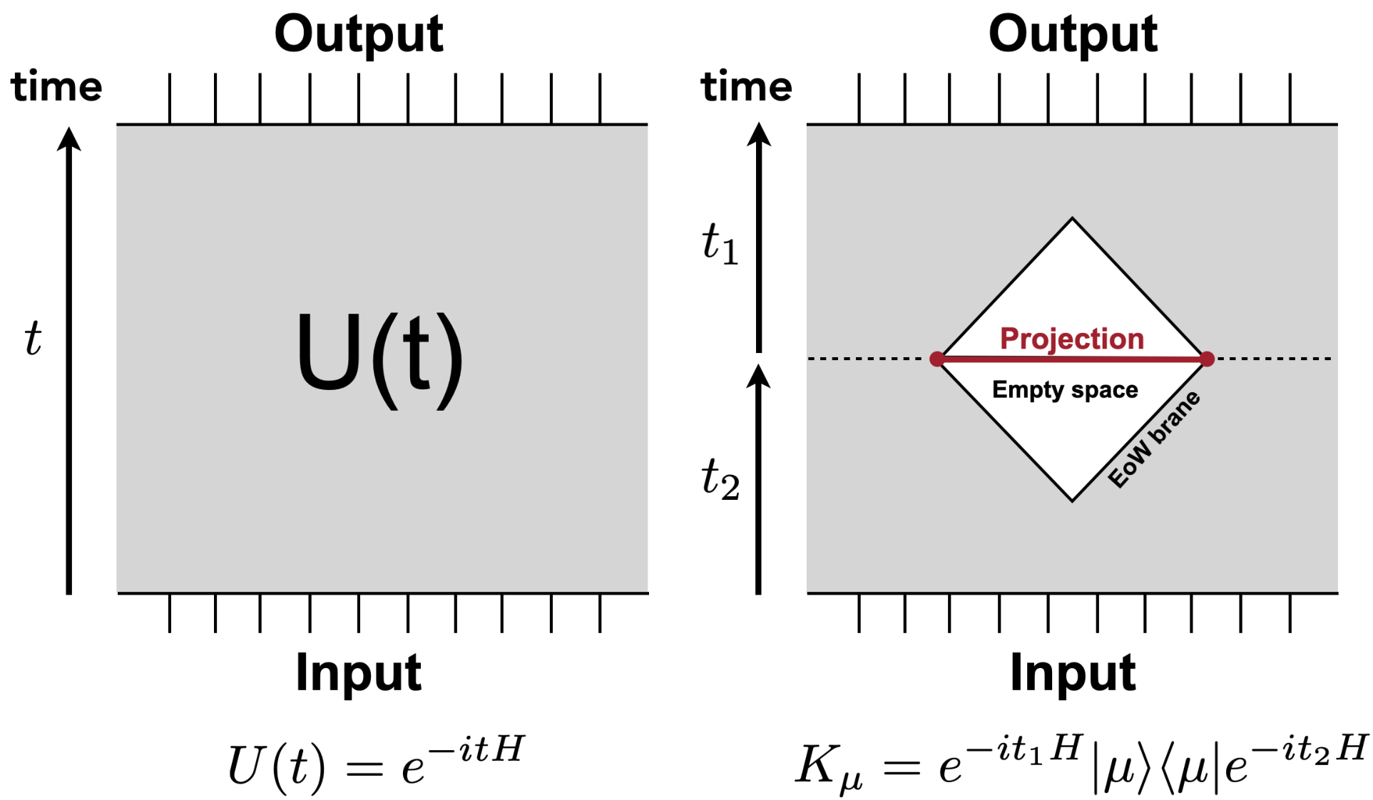
Figure 5: Quantum circuits with (right)/without (left) a projective measurement.

Line-Tension Picture with a Projective Measurement
Here we will explain a generalization of the simplest example of the line-tension picture described above to the system with a projective measurement. In this paper, the state is projected to a boundary state with no spatial entanglement in the coarse-grained limit ϵ→0\epsilon\rightarrow 0. In a unitary circuit, the state with no entanglement can be represented as an empty space. Since we expect that the unitary time-evolution makes the entanglement spread causally, the empty space with no entanglement shrinks according to the light-cone associated to the projected interval, thus the non-unitary quantum circuit consisting of two unitary time evolution operators and a projective measurement

Kμ=e−i​t1​H​|μ⟩​⟨μ|​e−i​t2​H\displaystyle K_{\mu}=e^{-it_{1}H}|\mu\rangle\langle\mu|e^{-it_{2}H} (4.5)

can be represented as Fig. 5.

4.2 Time dependence of OEE

Refer to caption
Figure 6: Configuration with trivial entanglement in line-tension picture.

Here we will explain how the operator entanglement computed using the line-tension picture that we proposed in this paper can reproduce the holographic results. Employing the line-tension picture in the unitary circuit proposed above (Fig. 5), we can reproduce the behavior of the entanglement computed in the previous section in the coarse-grained limit. There are non-trivial configurations of the minimal curves due to the existence of the projected region in the unitary circuit. In the case where the endpoint XX of the subregion at t=0t=0 is inside the projected region with no entanglement, the entanglement associated to a curve 𝒞0{\cal C}_{0} anchored at XX as in Fig. 6 becomes zero

S𝒞0=0.\displaystyle S_{{\cal C}_{0}}=0\,. (4.6)
Refer to caption
Figure 7: Three configurations in line-tension picture.

There are also several characteristic configurations of the minimal curves in the case where the endpoint XX of the subregion at t=0t=0 is outside the projected region. In Fig. 7, we drew such configurations 𝒞1,𝒞2{\cal C}_{1},{\cal C}_{2},and 𝒞3{\cal C}_{3} anchored at XX, which lies outside the projected region at t=0t=0, and the“end-of-the-world brane”, the boundary of the projected region. The entanglement SCiS_{C_{i}} associated to a curve 𝒞i{\cal C}_{i} can be computed as

S𝒞1\displaystyle S_{{\cal C}_{1}} =c​π12​ϵ​(P2−X),\displaystyle=\frac{c\pi}{12\epsilon}(P_{2}-X)\,, (4.7)
S𝒞2\displaystyle S_{{\cal C}_{2}} =c​π12​ϵ​(t2+P2−X2),\displaystyle=\frac{c\pi}{12\epsilon}\left(\frac{t}{2}+\frac{P_{2}-X}{2}\right)\,, (4.8)
S𝒞3\displaystyle S_{{\cal C}_{3}} =c​π12​ϵ​(t+P2−P12).\displaystyle=\frac{c\pi}{12\epsilon}\left(t+\frac{P_{2}-P_{1}}{2}\right)\,. (4.9)

In particular, the time-growth S𝒞2=c​π6​β​tS_{{\cal C}_{2}}=\frac{c\pi}{6\beta}t is a characteristic behavior not seen in the absence of the projection.

Here we will demonstrate how the holographic calculations of the operator entanglement entropy are correctly reproduced for Cases 3 and 4.
Case 3
Here, the subsystem BB and the projective measurement are located such that

0<X2<P2<P1<X1,X1−P2>P1−X2>X1−P1>P2−X2>0\displaystyle 0<X_{2}<P_{2}<P_{1}<X_{1},X_{1}-P_{2}>P_{1}-X_{2}>X_{1}-P_{1}>P_{2}-X_{2}>0 (4.10)

In this configuration, the time evolution of SBS_{B} computed in the line-tension picture (Fig. 8) is

SB≈{c​π​[(X1−X2)−(P1−P2)]12​ϵP2−X2>t2>0c​π​[t2−2​(P1−X1)−(X2−P2)]24​ϵX1−P1>t2>P2−X2c​π​[2​t2−(P1−P2)+(X1−X2)]24​ϵP1−X2>t2>X1−P1c​π​[3​t2−2​P1+X1+P2]24​ϵX1+2​P1−2​X2−P23>t2>P1−X2c​π​[X1−X2]12​ϵt2>X1+2​P1−2​X2−P23\displaystyle S_{B}\approx\begin{cases}\frac{c\pi\left[\left(X_{1}-X_{2}\right)-\left(P_{1}-P_{2}\right)\right]}{12\epsilon}&P_{2}-X_{2}>t_{2}>0\\ \frac{c\pi\left[t_{2}-2\left(P_{1}-X_{1}\right)-\left(X_{2}-P_{2}\right)\right]}{24\epsilon}&X_{1}-P_{1}>t_{2}>P_{2}-X_{2}\\ \frac{c\pi\left[2t_{2}-\left(P_{1}-P_{2}\right)+\left(X_{1}-X_{2}\right)\right]}{24\epsilon}&P_{1}-X_{2}>t_{2}>X_{1}-P_{1}\\ \frac{c\pi\left[3t_{2}-2P_{1}+X_{1}+P_{2}\right]}{24\epsilon}&\frac{X_{1}+2P_{1}-2X_{2}-P_{2}}{3}>t_{2}>P_{1}-X_{2}\\ \frac{c\pi\left[X_{1}-X_{2}\right]}{12\epsilon}&t_{2}>\frac{X_{1}+2P_{1}-2X_{2}-P_{2}}{3}\end{cases} (4.11)
Refer to caption
Figure 8: Diagrams in the line-tension picture in Case 3.

This correctly reproduces the leading order behavior of the entanglement entropy in the coarse-grained limit ϵ→0\epsilon\rightarrow 0.
Case 4
We take the locations of BB and the projective measurement to be

P1>X1>P2>X2>0,P1−X1>0,X1−P2>0,\displaystyle P_{1}>X_{1}>P_{2}>X_{2}>0,P_{1}-X_{1}>0,X_{1}-P_{2}>0, (4.12)
P1−X2>P1−X1>P2−X2>X1−P2>0\displaystyle P_{1}-X_{2}>P_{1}-X_{1}>P_{2}-X_{2}>X_{1}-P_{2}>0

In this configuration, the time evolution of SBS_{B} computed in the line-tension picture (Fig. 9) is

SB≈{π⁡(P2−X2)12​ϵX1−P2>t2>0c​π​[2​(P2−X2)+t2−(X1−P2)]24​ϵP2−X2>t2>X1−P2c​π​[(P2−X2)+2​t2−(X1−P2)]24​ϵP1−X1>t2>P2−X2c​π​[(P2−X2)+3​t2−(P1−P2)]24​ϵ2​(X1−P2)+P1−X23>t2>P1−X1c​π​(X1−X2)12​ϵt2>2​(X1−P2)+P1−X23\displaystyle S_{B}\approx\begin{cases}\ \frac{\pi\left(P_{2}-X_{2}\right)}{12\epsilon}&X_{1}-P_{2}>t_{2}>0\\ \frac{c\pi\left[2\left(P_{2}-X_{2}\right)+t_{2}-\left(X_{1}-P_{2}\right)\right]}{24\epsilon}&P_{2}-X_{2}>t_{2}>X_{1}-P_{2}\\ \frac{c\pi\left[\left(P_{2}-X_{2}\right)+2t_{2}-\left(X_{1}-P_{2}\right)\right]}{24\epsilon}&P_{1}-X_{1}>t_{2}>P_{2}-X_{2}\\ \frac{c\pi\left[\left(P_{2}-X_{2}\right)+3t_{2}-\left(P_{1}-P_{2}\right)\right]}{24\epsilon}&\frac{2\left(X_{1}-P_{2}\right)+P_{1}-X_{2}}{3}>t_{2}>P_{1}-X_{1}\\ \frac{c\pi\left(X_{1}-X_{2}\right)}{12\epsilon}&t_{2}>\frac{2\left(X_{1}-P_{2}\right)+P_{1}-X_{2}}{3}\end{cases} (4.13)

for the case 2​(P1−X1)−(P2−X2)<3​(X1−P2)2\left(P_{1}-X_{1}\right)-\left(P_{2}-X_{2}\right)<3\left(X_{1}-P_{2}\right). The line-tension picture once again correctly reproduces the leading order behavior of the entanglement entropy in the coarse-grained limit ϵ→0\epsilon\rightarrow 0.

Refer to caption
Figure 9: Diagrams for the line-tension picture in Case 4.

5 Gravitational description

We have discussed operator entanglement for projection operators in holographic CFTs. In this section, we investigate the bulk spacetime which is relevant to our projection operator state. The gravity picture is also consistent with the light-cone structure of EOW brane discussed in Section 4.

5.1 Projection and the AdS/BCFT correspondence

Recall that operator states are defined as maximally entangled states acted upon by the operator of interest,

|𝒪A⟩≡𝒪A⊗1B∑n|nAnB∗⟩,\displaystyle|{\mathcal{O}_{A}}\rangle\equiv\mathcal{O}_{A}\otimes 1_{B}\sum_{n}|{n_{A}n^{\ast}_{B}}\rangle, (5.1)

where we omit the normalization constant. Note that the maximally entangled state is equivalent to the (infinite temperature) TFD state,

|TFDβ⟩=∑ne−β2​En​|nA​nB∗⟩,\displaystyle|{\text{TFD}_{\beta}}\rangle=\sum_{n}\mathrm{e}^{-\frac{\beta}{2}E_{n}}|n_{A}n^{\ast}_{B}\rangle, (5.2)

which is holographically dual to an eternal black hole in AdS. Therefore, our projection operator state (with UV regulator ϵ\epsilon) can be written as

|Kμ⟩=e−ϵ​H​𝒫μ​|TFD2​ϵ⟩,\displaystyle|{K_{\mu}}\rangle=\mathrm{e}^{-\epsilon H}\mathcal{P}_{\mu}|{\text{TFD}_{2\epsilon}}\rangle, (5.3)

where 𝒫μ\mathcal{P}_{\mu} is the projection operator acting on a certain spatial subsystem VV and HH is the Hamiltonian of the system. We need to take into account the effect of the spatial projection 𝒫μ\mathcal{P}_{\mu} in the eternal black hole geometry. Since the Euclidean path integral treats the spatial projections as slits, we can discuss the dual gravity picture based on the AdS/BCFT correspondence [35, 36]. In light of AdS/BCFT, we expect that in the gravity picture, such spatial projections introduce an end-of-the-world (EOW) brane in the bulk.

We are interested in Einstein gravity on a bulk spacetime MM coupled to matter fields on a dynamical brane QQ,

S=116​π​GN​∫M−g​(R−2​Λ)+18​π​GN​∫∂M∪Q−h​K+SQ,\displaystyle S=\dfrac{1}{16\pi G_{N}}\int_{M}\sqrt{-g}(R-2\Lambda)+\dfrac{1}{8\pi G_{N}}\int_{\partial M\cup Q}\sqrt{-h}K+S_{Q}, (5.4)

where SQS_{Q} denotes matter contributions localized on the dynamical brane QQ. The second term is a Gibbons-Hawking boundary term for ∂M\partial M and QQ. In contrast with the standard Dirichlet boundary condition on the asymptotic boundary δ​gμ​ν=0\delta g_{\mu\nu}=0, we will impose the Neumann-type boundary condition on QQ so that the metric on QQ remains dynamical,

Ki​j−hi​j​K=−16​π​GN−h​δ​SQδ​hi​j≡Ti​jQ.\displaystyle K_{ij}-h_{ij}K=-\dfrac{16\pi G_{N}}{\sqrt{-h}}\dfrac{\delta S_{Q}}{\delta h^{ij}}\equiv T^{Q}_{ij}. (5.5)

In principle, we would solve (5.5) for a given matter action SQS_{Q} and determine the properties of the brane QQ. In bottom up models of AdS/BCFT, we assume that

Ti​jQ=−T​hi​j,\displaystyle T^{Q}_{ij}=-Th_{ij}, (5.6)

where TT is a constant tension for the brane. In this way, we can preserve the boundary conformal symmetry. The brane QQ is often called the end-of-the-world (EOW) brane.

As in the previous section, we will be particularly interested in the situation where the EOW brane is tensionless, i.e. T=0T=0. Since the extrinsic curvature becomes trivial in this case, Ki​j=0K_{ij}=0, the EOW brane becomes a totally geodesic surface. After the conformal map discussed in Section 2, our computation reduces to the holographic entanglement entropy for the standard Hartman-Maldacena geometry. One can check that this reproduces the CFT results in Section 3.

5.2 Holographic entanglement entropy in a simpler setup

We may view our setup as a generalization of the Hartman-Maldacena geometry. From this point of view, the new ingredient is a finite size EOW brane inside the horizon. This quantitatively changes the time evolution of the entanglement entropy. As we have already seen, the linear growth in time can become milder than in the stardard Hartman-Maldacena geometry in the middle time regime. It is given by

Sdis.=α02​t+⋯,\displaystyle S_{\text{dis.}}=\dfrac{\alpha_{0}}{2}t+\cdots, (5.7)

where

α0=c​π3​β,\displaystyle\alpha_{0}=\dfrac{c\pi}{3\beta}, (5.8)

is the coefficient in the ordinary Hartman-Maldacena geometry. Here, we took the large black hole limit, i.e. the high temperature limit, so that the linear growth is manifest. The remaining terms denoted by dots are the sub-leading terms in this limit.

In light of the line-tension picture, we understand that this difference comes from the light-cone structure of the EOW brane. Here, we attempt to understand the origin of the additional factor of 1/21/2 in a simpler setup in the bulk. To accomplish this, let us consider the single-sided setup (see Figure 10). Note that if we take the large black hole limit, the difference between the previous setup and the current setup is sub-leading.

Refer to caption
Figure 10: Euclidean geometry for computing the minimal area surface in Section 5.2. We omit the lower half of the Euclidean geometry (τE<0\tau_{E}<0 part) as the geometry is time-reflection symmetric.

Setup and computation of the minimal area surface

For simplicity, we focus on the entanglement entropy of a semi-infinite line A=[−∞,X]A=[-\infty,X]. Based on the prescription of holographic entanglement entropy, we would like to compute the extremal surface connecting the EOW brane and a boundary point XX. Since the tensionless EOW brane is a totally geodesic submanifold, we can view the domain of the EOW brane as geodesics anchored on the boundary of the projection. Using this fact, one can find the extremal surface as the minimal geodesics between EOW (i.e., geodesics anchored on the boundary of the projection) and the boundary point. After the computation, we will analytically continue to the Lorenzian time.

For this purpose, it is useful to utilize the embedding formalism. Namely, we view vacuum solutions in three dimensional Einstein gravity with the negative cosmological constant as submanifolds in ℝ1,3\mathbb{R}^{1,3},

X2\displaystyle X^{2} ≡X⋅X=−1,\displaystyle\equiv X\cdot X=-1, (5.9)
ηA​B\displaystyle\eta_{AB} =diag⁡(−1,1,1,1),\displaystyle=\mathrm{diag}(-1,1,1,1), (5.10)

and its quotient. Here, we introduced the inner product in the embedding space as

X⋅Y≡ηA​B​XA​YB.\displaystyle X\cdot Y\equiv\eta_{AB}X^{A}Y^{B}. (5.11)

The spacelike geodesics γi​j\gamma_{ij} in the embedding space ℝ1,3\mathbb{R}^{1,3} are given by

Xi​jA​(λ)=PiA​e−λ+PjA​eλ−2Pi⋅Pj,\displaystyle X_{ij}^{A}(\lambda)=\dfrac{P_{i}^{A}\mathrm{e}^{-\lambda}+P_{j}^{A}\mathrm{e}^{\lambda}}{\sqrt{-2P_{i}\cdot P_{j}}}, (5.12)

where λ\lambda is “proper time” which runs from −∞-\infty to ∞\infty and Pi,jAP_{i,j}^{A} are the geodesic boundary coordinates in the embedding space,

Pi,jA\displaystyle P_{i,j}^{A} =(cosh⁡r+​Pi,j,sin⁡r+​τi,j,sinh⁡r+​Pi,j,cos⁡r+​τi,j).\displaystyle=(\cosh r_{+}P_{i,j},\sin r_{+}\tau_{i,j},\sinh r_{+}P_{i,j},\cos r_{+}\tau_{i,j}). (5.13)

Now we can use this spacelike geodesics as the coordinates of the EOW brane. We then extremize the geodesic length between the EOW brane and XX with respect to λ\lambda. Assuming XX is on the cutoff surface of the asymptotic AdS, we obtain the geodesic length as

L(λext)≃log(−2Xi​j(λext)⋅X),\displaystyle L(\lambda_{\text{ext}})\simeq\log(-2X_{ij}(\lambda_{\text{ext}})\cdot X), (5.14)

where

−2Xi​j(λext.)⋅X=2(−2P1⋅X)(−2P2⋅X)(−2P1⋅P2)(−2P1⋅P2).\displaystyle-2X_{ij}(\lambda_{\text{ext.}})\cdot X=2\sqrt{\dfrac{(-2P_{1}\cdot X)(-2P_{2}\cdot X)}{(-2P_{1}\cdot P_{2})(-2P_{1}\cdot P_{2})}}. (5.15)

Here, P1P_{1} and P2P_{2} are the embedding coordinates of the boundary of the projection, and XX is the boundary of the subsystem AA (on the bulk cutoff surface),

XA\displaystyle X^{A} ≃r∞r+(coshr+X,sinr+τX,sinhr+X,cosr+τX).\displaystyle\simeq\dfrac{r_{\infty}}{r_{+}}(\cosh r_{+}X,\sin r_{+}\tau_{X},\sinh r_{+}X,\cos r_{+}\tau_{X}). (5.16)

Note that we are using the bulk counterpart of the boundary coordinates XAX^{A} (which is on the cutoff surface r=r∞r=r_{\infty}).

Figure 11: Time dependence of the holographic entanglement entropy given by (5.17) (with 4​GN=14G_{N}=1) for small and large r+r_{+}, as a function of tt. Here we took X=0,P1=14,P2=2X=0,P_{1}=14,P_{2}=2 and r∞=100r_{\infty}=100. For the plot, we recover the constant term 12​log⁡(2​r∞/r+)\frac{1}{2}\log(2r_{\infty}/r_{+}).

After the analytic continuation to the Lorenzian signature τ→i​t\tau\rightarrow it, we obtain

L\displaystyle L ≃12​log⁡|sinh⁡(12​r+​(−P1+t+X))​sinh⁡(12​r+​(−P1−t+X))sinh⁡(12​r+​(P1−P2))|\displaystyle\simeq\frac{1}{2}\log\left|\frac{\sinh\left(\frac{1}{2}r_{+}(-P_{1}+t+X)\right)\sinh\left(\frac{1}{2}r_{+}(-P_{1}-t+X)\right)}{\sinh\left(\frac{1}{2}r_{+}(P_{1}-P_{2})\right)}\right|
+12​log⁡|sinh⁡(12​r+​(−P2−t+X))​sinh⁡(12​r+​(−P2+t+X))sinh⁡(12​r+​(P1−P2))|\displaystyle+\,\frac{1}{2}\log\left|\frac{\sinh\left(\frac{1}{2}r_{+}(-P_{2}-t+X)\right)\sinh\left(\frac{1}{2}r_{+}(-P_{2}+t+X)\right)}{\sinh\left(\frac{1}{2}r_{+}(P_{1}-P_{2})\right)}\right| (5.17)

where we omit a constant term 12​log⁡(2​r∞/r+)\frac{1}{2}\log(2r_{\infty}/r_{+}) as we are interested in the large r+r_{+} limit. This expression gives the time-evolution of the holographic entanglement entropy (see Figure 11).

Time dependence of the minimal surface area

The leading piece in the large r+r_{+} limit of the area of the minimal surface (5.17) is given by

L\displaystyle L ≃r+4​(|X−t−P1|+|X+t−P1|+|X−t−P2|+|X+t−P2|−2​|P1−P2|).\displaystyle\simeq\dfrac{r_{+}}{4}(|X-t-P_{1}|+|X+t-P_{1}|+|X-t-P_{2}|+|X+t-P_{2}|-2|P_{1}-P_{2}|). (5.18)

As a concrete example, let us assume that X<P2<P1X<P_{2}<P_{1}. In this case, we obtain

SA=L4​GN≃{c​π3​β​(P2−X)(0<t<P2−X),c​π6​β​(t+P2−X)(P2−X<t<P1−X),c​π6​β​(2​t+P2−P1)(P1−X<t).\displaystyle S_{A}=\frac{L}{4G_{N}}\simeq\begin{cases}\frac{c\pi}{3\beta}(P_{2}-X)&(0<t<P_{2}-X),\\ \frac{c\pi}{6\beta}(t+P_{2}-X)&(P_{2}-X<t<P_{1}-X),\\ \frac{c\pi}{6\beta}\left(2t+P_{2}-P_{1}\right)&(P_{1}-X<t).\end{cases} (5.19)

Here, we used the standard AdS/CFT dictionary,

r+4​GN=c​π3​β.\displaystyle\frac{r_{+}}{4G_{N}}=\dfrac{c\pi}{3\beta}. (5.20)

By identifying β=4​ϵ\beta=4\epsilon, we reproduce the results of the holographic CFT and the line-tension picture calculations. Furthermore, one can confirm that the motion of the minimal surface is also consistent with the line-tension picture (see Figure 12).

Note that this simple setup should be universal in any 22d CFT. In particular, the increase of entanglement can be understood as the propagation of EPR pairs from the each point of the projection.

Figure 12: Time dependence of trajectory of the minimal surface with X=0,P1=14,P2=2X=0,P_{1}=14,P_{2}=2 as a function of tt. We plot how the xx-coordinates of endpoint of the minimal area surface move under the time-evolution. The large r+r_{+} regime (solid blue curve) is consistent with the line-tension picture. In this setup, it starts at X=P2X=P_{2} (edge) and finally stops at X=(P1+P2)/2X=(P_{1}+P_{2})/2 (center).

6 Discussions and Future directions

In this paper, we discussed the effect of a single projective measurement on the dynamics of 22d holographic CFTs. It is shown that when the projective measurement is performed at a certain time in the holographic CFTs, the dual gravitational bulk is given by an AdS spacetime with an end-of-the-world brane at the corresponding time slice. We also proposed a line tension model that effectively describes the effect of projective measurement on entanglement in a chaotic system. It is an interesting future direction to extend our analysis to the case of multiple projective measurements. It can be seen from (4.6) and (4.7) that a single projective measurement stops the non-trivial time evolution of the subsystem for a certain finite time, depending on the size of the subsystem and its location relative to the measurement. If the line tension picture for a single projective measurement we proposed in this paper is straightforwardly applicable to the case of multiple projective measurements, it is expected that by keeping the time interval between each projective measurement sufficiently short, the subsystem will not evolve in time at all. This can be thought of as a realization of the quantum Zeno effect in quantum mechanics, in which repeated observations cause the system to freeze. If this line tension picture is correct and reflects the geometrical structure in the gravity dual, the corresponding spacetime is expected to be the AdS spacetime with multiple branes inserted. However, the backreaction due to the insertion of multiple measurements cannot be ignored in general, and the AdS spacetime itself may be deformed significantly11 1 We thank Tadashi Takayanagi for pointing out this possibility.. We will leave it to future studies to elucidate what spacetime is realized and what line tension picture appropriately reflects the spacetime in the case of multiple measurements.

Future directions

Here are a few possible future directions:

  • •

    Single projective measurement in free CFTs: In this paper, we studied how a single projective measurement of finite size affects quantum dynamics with maximal information scrambling. We expect that the effect of the projective measurement on the unitary time evolution will depend on the degree of information scrambling generated by the dynamics. The dynamics of the unitary time evolution in the 22d free fermion can be described by relativistic propagation of quasi-particles [20, 24]. It would be interesting to study how this effective picture is modified when a finite-size projective measurement is included in the quantum circuit.

  • •

    Relation to the random projective measurement: In a quantum circuit with a random arrangement of projective measurements acting on a single site, it was discovered that an area law-volume law phase transition of the OEE occurs, depending on the frequency of these projections. However, such a phase transition did not occur in a 22d holographic system containing only one projective measurement of finite size. It would be interesting to study whether such a phase transition occurs when a 22d holographic system contains randomly placed projective measurements.

Acknowledgements

We thank useful discussions with Jonah Kudler-Flam, Shinsei Ryu, and Tadashi Takayanagi. K.G. is supported by JSPS KAKENHI Grant-in-Aid for Early-Career Scientists (21K13930) and Research Fellowships of Japan Society for the Promotion of Science for Young Scientists (22J00663). M.N. is supported by funds from the University of Chinese Academy of Sciences (UCAS), funds from the Kavli Institute for Theoretical Sciences (KITS). K.T. is supported by JSPS KAKENHI Grant No. 21K13920 and MEXT KAKENHI Grant No. 22H05265. This material is based upon work supported by the National Science Foundation under Grant No. NSF-DMR 2018358 and by an appointment to the YST Program at the APCTP through the Science and Technology Promotion Fund and Lottery Fund of the Korean Government, as well as the Korean Local Governments - Gyeongsangbuk-do Province and Pohang City (MT).

Appendix A The time-dependence of OEE for various subsystems

In Appendix A, we will explain the time evolution of SBS_{B} for cases excluding Case 4. By replacing t2t_{2} of SBS_{B} with t1t_{1}, the time evolution of SAS_{A} is given by that of SBS_{B}.

A.1 Case 1

Let us first consider the simplest case where the location of A,BA,B and the projective measurement at t1=t2=0t_{1}=t_{2}=0 are on the top of each other:

P1=X1=Y1,P2=X2=Y2P_{1}=X_{1}=Y_{1},P_{2}=X_{2}=Y_{2} (A.1)

A.1.1 The time-dependence of OEE

In this case, let us look closely at the time-dependence of OEE in the large measurement limit, P1−P2≫ϵP_{1}-P_{2}\gg\epsilon. In this limit, the contribution from the conformal factor is approximated by

limn→1hn1−n​log⁡[∏i=1,2d​𝒲​(wi)d​wi​d​𝒲¯​(wi)d​w¯i]≈c6​log⁡[X1−X22​ϵ]−c3​log⁡(π2​ϵ)+c12×{π​t2ϵfor​X1−X2>t2≥0π⁡(2​t2−(X1−X2)CLOSEϵfor​t2>X1−X2\begin{split}&\lim_{n\rightarrow 1}\frac{h_{n}}{1-n}\log{\left[\prod_{i=1,2}\frac{d\mathcal{W}(w_{i})}{dw_{i}}\frac{d\overline{\mathcal{W}}(w_{i})}{d\overline{w}_{i}}\right]}\\ &\approx\frac{c}{6}\log{\left[\frac{X_{1}-X_{2}}{2\epsilon}\right]}-\frac{c}{3}\log{\left(\frac{\pi}{2\epsilon}\right)}+\frac{c}{12}\times\begin{cases}\frac{\pi t_{2}}{\epsilon}~&~\text{for}~X_{1}-X_{2}>t_{2}\geq 0\\ \frac{\pi(2t_{2}-(X_{1}-X_{2})}{\epsilon}~&~\text{for}~t_{2}>X_{1}-X_{2}\end{cases}\end{split} (A.2)

Then, consider the time-dependence of the non-universal pieces of the OEE for the single interval. As in Case 4, SB,conS_{B,\text{con}} is independent of t2t_{2}, while the time-dependence of SB,disS_{B,\text{dis}} is given by

SB,dis≈−c6​log⁡(X1−X2ϵ)+c12×{π⁡(X1−X2−t2)ϵfor​X1−X2>t2>0−2​π​(t2−(X1−X2))ϵfor​t2>X1−X2.\begin{split}&S_{\text{B,dis}}\approx-\frac{c}{6}\log{\left(\frac{X_{1}-X_{2}}{\epsilon}\right)}+\frac{c}{12}\times\begin{cases}\frac{\pi(X_{1}-X_{2}-t_{2})}{\epsilon}&~\text{for}~X_{1}-X_{2}>t_{2}>0\\ \frac{-2\pi(t_{2}-(X_{1}-X_{2}))}{\epsilon}&~\text{for}~t_{2}>X_{1}-X_{2}\\ \end{cases}.\\ \end{split} (A.3)

The time-dependence of non-universal piece of SBS_{B} is given by

SB,Non-uni.=Min​[SB,con,SB,dis]≈−c6​log⁡(X1−X2ϵ)+{0X1−X2>t2>0−2​π​(t2−(X1−X2))ϵt2>X1−X2,\begin{split}&S_{\text{B,Non-uni.}}=\text{Min}\left[S_{\text{B,con}},S_{\text{B,dis}}\right]\approx-\frac{c}{6}\log{\left(\frac{X_{1}-X_{2}}{\epsilon}\right)}+\begin{cases}0&X_{1}-X_{2}>t_{2}>0\\ \frac{-2\pi(t_{2}-(X_{1}-X_{2}))}{\epsilon}&t_{2}>X_{1}-X_{2}\end{cases},\\ \end{split} (A.4)

where in the early-time region, X1−X2>t2>0X_{1}-X_{2}>t_{2}>0, the non-universal piece of SBS_{B} is determined by SB,conS_{B,\text{con}} while in the late time region, t2>X1−X2t_{2}>X_{1}-X_{2}, that of SBS_{B} is determined by SB,disS_{B,\text{dis}}.

Consequently, the time evolution of SBS_{B} is given by

SB≈c3​log⁡(2​ϵπ)+c​π12​ϵ×{t2X1−X2>t2>0X1−X2t2>X1−X2.\begin{split}&S_{B}\approx\frac{c}{3}\log{\left(\frac{2\epsilon}{\pi}\right)}+\frac{c\pi}{12\epsilon}\times\begin{cases}t_{2}&X_{1}-X_{2}>t_{2}>0\\ X_{1}-X_{2}&t_{2}>X_{1}-X_{2}\\ \end{cases}.\\ \end{split} (A.5)

In this case, the projective measurement acts on the whole region of BB. Then, the initial value of SBS_{B} is approximately zero, except for c3​log⁡(2​ϵπ)\frac{c}{3}\log{\left(\frac{2\epsilon}{\pi}\right)}. Since the size of the projective measurement is the same as that of BB, the scrambling effect of the time evolution operator increases the amount of SBS_{B} from the beginning, t2=0t_{2}=0. In the late-time region, t2>X1−X2t_{2}>X_{1}-X_{2}, SBS_{B} becomes the entanglement entropy of the thermal state where the inverse temperature is 4​ϵ4\epsilon.

A.2 Case 2

Second, let us study how the projective measurement far from the subsystems contributes to the time evolution of OEE for those subsystems. To do so, consider the case where the spatial location of the projective measurement is far from that of the subsystems, AA and BB, at t1=t2=0t_{1}=t_{2}=0:

P1>P2>X1=Y1>X2=Y2>0.P_{1}>P_{2}>X_{1}=Y_{1}>X_{2}=Y_{2}>0. (A.6)

The time-dependence of OEE

Here, we turn to the analysis on the time-dependence of the universal pieces in two subcases: P1−P2>X1−X2>0P_{1}-P_{2}>X_{1}-X_{2}>0 and X1−X2>P1−P2X_{1}-X_{2}>P_{1}-P_{2}.

A.2.1 P1−P2>X1−X2>0P_{1}-P_{2}>X_{1}-X_{2}>0

In the case of P1−P2>X1−X2>0P_{1}-P_{2}>X_{1}-X_{2}>0, the contribution from the global structure of the torus should be in the large measurement limit since we are taking the coarse grained limit. Thus, the time evolution of the universal piece is given by

limn→1hn1−n​log⁡[Πi=1,2​d​𝒲​(wi)d​wi​d​𝒲¯​(wi)d​w¯i]=c6​log⁡(P1−P2ϵ)\begin{split}&\lim_{n\rightarrow 1}\frac{h_{n}}{1-n}\log{\left[\Pi_{i=1,2}\frac{d\mathcal{W}(w_{i})}{dw_{i}}\frac{d\overline{\mathcal{W}}(w_{i})}{d\overline{w}_{i}}\right]}=\frac{c}{6}\log{\left(\frac{P_{1}-P_{2}}{\epsilon}\right)}\end{split} (A.7)

In the limit, P1−P2≫ϵP_{1}-P_{2}\gg\epsilon, the contribution from the conformal factor is approximated by

limn→1hn1−n​log⁡[Πi=1,2​d​𝒲​(wi)d​wi​d​𝒲¯​(wi)d​w¯i]≈c6​log⁡(P1−P2ϵ)−c3​log⁡(π2​ϵ)+c24×{(2​π​(2​P2−X1−X2)ϵ)P2−X1>t2>0π⁡(3​P2−X1−2​X2+t2)ϵP2−X2>t2>P2−X1π⁡(2​P2−X1−X2+2​t2)ϵP1−X1>t2>P2−X2π⁡(−P1+2​P2−X2+3​t2)ϵP1−X2>t2>P1−X12​π​(−P1+P2+2​t2)ϵt2>P1−X2.\begin{split}&\lim_{n\rightarrow 1}\frac{h_{n}}{1-n}\log{\left[\Pi_{i=1,2}\frac{d\mathcal{W}(w_{i})}{dw_{i}}\frac{d\overline{\mathcal{W}}(w_{i})}{d\overline{w}_{i}}\right]}\approx\frac{c}{6}\log{\left(\frac{P_{1}-P_{2}}{\epsilon}\right)}-\frac{c}{3}\log{\left(\frac{\pi}{2\epsilon}\right)}\\ &+\frac{c}{24}\times\begin{cases}\left(\frac{2\pi(2P_{2}-X_{1}-X_{2})}{\epsilon}\right)&P_{2}-X_{1}>t_{2}>0\\ \frac{\pi(3P_{2}-X_{1}-2X_{2}+t_{2})}{\epsilon}&P_{2}-X_{2}>t_{2}>P_{2}-X_{1}\\ \frac{\pi(2P_{2}-X_{1}-X_{2}+2t_{2})}{\epsilon}&P_{1}-X_{1}>t_{2}>P_{2}-X_{2}\\ \frac{\pi(-P_{1}+2P_{2}-X_{2}+3t_{2})}{\epsilon}&P_{1}-X_{2}>t_{2}>P_{1}-X_{1}\\ \frac{2\pi(-P_{1}+P_{2}+2t_{2})}{\epsilon}&t_{2}>P_{1}-X_{2}\\ \end{cases}.\\ \end{split} (A.8)

The value of SB,conS_{B,\text{con}} is independent of t2t_{2} and is given by (3.8), while the time-dependence of SB,disS_{\text{B,dis}} is given by

SB,dis≈−c6​log⁡(P1−P2ϵ)+c12×{(−2​π​(P2−X1)ϵ)P2−X1>t2>0(−π⁡(t2+3​(P2−X1))2​ϵ)P2−X2>t2>P2−X1(π⁡[X1−X2−2​(P2−X1)−2​t2]2​ϵ)P1−X1>t2>P2−X2(π⁡[P1−X2−2​(P2−X1)−3​t2]2​ϵ)P1−X2>t2>P1−X1(π⁡[P1−X2−(P2−X1)−2​t2]ϵ)t2>P1−X2,\begin{split}&S_{\text{B,dis}}\approx-\frac{c}{6}\log{\left(\frac{P_{1}-P_{2}}{\epsilon}\right)}+\frac{c}{12}\times\begin{cases}\left(\frac{-2\pi(P_{2}-X_{1})}{\epsilon}\right)&P_{2}-X_{1}>t_{2}>0\\ \left(\frac{-\pi(t_{2}+3(P_{2}-X_{1}))}{2\epsilon}\right)&P_{2}-X_{2}>t_{2}>P_{2}-X_{1}\\ \left(\frac{\pi\left[X_{1}-X_{2}-2(P_{2}-X_{1})-2t_{2}\right]}{2\epsilon}\right)&P_{1}-X_{1}>t_{2}>P_{2}-X_{2}\\ \left(\frac{\pi\left[P_{1}-X_{2}-2(P_{2}-X_{1})-3t_{2}\right]}{2\epsilon}\right)&P_{1}-X_{2}>t_{2}>P_{1}-X_{1}\\ \left(\frac{\pi\left[P_{1}-X_{2}-(P_{2}-X_{1})-2t_{2}\right]}{\epsilon}\right)&t_{2}>P_{1}-X_{2}\end{cases},\\ \end{split} (A.9)

where the value of SB,conS_{B,\text{con}} is always larger than that of SB,disS_{B,\text{dis}}. Therefore, SB,Non-uni.S_{B,\text{Non-uni.}} is determined by SB,disS_{B,\text{dis}}. Thus, SBS_{B} is independent of t1t_{1} and t2t_{2}, and its value is given by

SB≈c3​log⁡(2​ϵπ)+c​π​(X1−X2)12​ϵ.\begin{split}S_{B}\approx\frac{c}{3}\log{\left(\frac{2\epsilon}{\pi}\right)}+\frac{c\pi(X_{1}-X_{2})}{12\epsilon}.\end{split} (A.10)

X1−X2>P1−P2>0X_{1}-X_{2}>P_{1}-P_{2}>0

In the case of X1−X2>P1−P2>0X_{1}-X_{2}>P_{1}-P_{2}>0, the universal piece in the large projection limit, P1−P2≫ϵP_{1}-P_{2}\gg\epsilon, is given by

limn→1hn1−n​log⁡[Πi=1,2​d​𝒲​(wi)d​wi​d​𝒲¯​(wi)d​w¯i]≈−c3​log⁡(π2​ϵ)+c6×{log⁡(P1−P2ϵ)P1−P2≫ϵlog⁡(12)ϵ≫P1−P2>0+c24×{(2​π​(2​P2−X1−X2)ϵ)P2−X1>t2>0π⁡(3​P2−X1−2​X2+t2)ϵP1−X1>t2>P2−X1π⁡(−P1+3​P2−2​X2+2​t2)ϵP2−X2>t2>P1−X1π⁡(−P1+2​P2−X2+3​t2)ϵP1−X2>t2>P2−X22​π​(−P1+P2+2​t2)ϵt2>P1−X2.\begin{split}&\lim_{n\rightarrow 1}\frac{h_{n}}{1-n}\log{\left[\Pi_{i=1,2}\frac{d\mathcal{W}(w_{i})}{dw_{i}}\frac{d\overline{\mathcal{W}}(w_{i})}{d\overline{w}_{i}}\right]}\approx-\frac{c}{3}\log{\left(\frac{\pi}{2\epsilon}\right)}+\frac{c}{6}\times\begin{cases}\log{\left(\frac{P_{1}-P_{2}}{\epsilon}\right)}&P_{1}-P_{2}\gg\epsilon\\ \log{\left(\frac{1}{2}\right)}&\epsilon\gg P_{1}-P_{2}>0\end{cases}\\ &+\frac{c}{24}\times\begin{cases}\left(\frac{2\pi(2P_{2}-X_{1}-X_{2})}{\epsilon}\right)&P_{2}-X_{1}>t_{2}>0\\ \frac{\pi(3P_{2}-X_{1}-2X_{2}+t_{2})}{\epsilon}&P_{1}-X_{1}>t_{2}>P_{2}-X_{1}\\ \frac{\pi(-P_{1}+3P_{2}-2X_{2}+2t_{2})}{\epsilon}&P_{2}-X_{2}>t_{2}>P_{1}-X_{1}\\ \frac{\pi(-P_{1}+2P_{2}-X_{2}+3t_{2})}{\epsilon}&P_{1}-X_{2}>t_{2}>P_{2}-X_{2}\\ \frac{2\pi(-P_{1}+P_{2}+2t_{2})}{\epsilon}&t_{2}>P_{1}-X_{2}\\ \end{cases}.\\ \end{split} (A.11)

In this case, the value of SB,conS_{B,\text{con}} is equal to (3.8) so the late time evolution of SB,disS_{\text{B,dis}} depends on t2t_{2} and is given by

SB,dis≈−c6​log⁡(P1−P2ϵ)+c12×{(−2​π​(P2−X1)ϵ)P2−X1>t1>0(−π⁡(t2+3​(P2−X1))2​ϵ)P1−X1>t1>P2−X1(π⁡[P1−P2−2​(P2−X1)−2​t2]2​ϵ)P2−X2>t1>P1−X1(π⁡[P1−X2−2​(P2−X1)−3​t2]2​ϵ)P1−X2>t1>P2−X2(π⁡[P1−X2−(P2−X1)−2​t2]ϵ)t1>P1−X2,\begin{split}&S_{\text{B,dis}}\approx-\frac{c}{6}\log{\left(\frac{P_{1}-P_{2}}{\epsilon}\right)}+\frac{c}{12}\times\begin{cases}\left(\frac{-2\pi(P_{2}-X_{1})}{\epsilon}\right)&P_{2}-X_{1}>t_{1}>0\\ \left(\frac{-\pi(t_{2}+3(P_{2}-X_{1}))}{2\epsilon}\right)&P_{1}-X_{1}>t_{1}>P_{2}-X_{1}\\ \left(\frac{\pi\left[P_{1}-P_{2}-2(P_{2}-X_{1})-2t_{2}\right]}{2\epsilon}\right)&P_{2}-X_{2}>t_{1}>P_{1}-X_{1}\\ \left(\frac{\pi\left[P_{1}-X_{2}-2(P_{2}-X_{1})-3t_{2}\right]}{2\epsilon}\right)&P_{1}-X_{2}>t_{1}>P_{2}-X_{2}\\ \left(\frac{\pi\left[P_{1}-X_{2}-(P_{2}-X_{1})-2t_{2}\right]}{\epsilon}\right)&t_{1}>P_{1}-X_{2}\\ \end{cases},\\ \end{split} (A.12)

where the value of SB,conS_{B,\text{con}} is always larger than that of SB,disS_{B,\text{dis}}, so that the time evolution of non-universal piece is determined by SB,disS_{B,\text{dis}}. As a consequence, the values of OEE are independent of t1t_{1} and t2t_{2}, and their values are given by (A.10).

A.3 Case 3

Next, we study how the projective measurement changes the time-dependence of OEE when the projective measurement is a subregion of the subsystems at t1=t2=0t_{1}=t_{2}=0. More precisely, we will study the time-dependence of OEE in the following configuration:

X1=Y1>P1>P2>X2=Y2>0,X1−P2>P1−X2>X1−P1>P2−X2>0.X_{1}=Y_{1}>P_{1}>P_{2}>X_{2}=Y_{2}>0,~X_{1}-P_{2}>P_{1}-X_{2}>X_{1}-P_{1}>P_{2}-X_{2}>0. (A.13)

A.3.1 Time-dependence of OEE

The time-dependence of the universal piece in Case 3 is given by

c24​log⁡[Πi=1,2​d​𝒲​(wi)d​wi​d​𝒲¯​(wi)d​w¯i]≈−c3​log⁡(π2​ϵ)+c6×{log⁡(P1−P2ϵ)P1−P2≫ϵlog⁡(12)ϵ≫P1−P2>0+c24×{(OPEN2​(X1−X2)−2​(P1−P2))ϵ)P2−X2>t2>0π⁡(P2−X2+2​(X1−P1)+t2)ϵX1−P1>t2>P2−X2π⁡(X1−X2−(P1−P2)+2​t2)ϵP1−X2>t2>X1−P1π⁡(X1−2​P1+P2+3​t2)ϵX1−P2>t2>P1−X22​π​(−P1+P2+2​t2)ϵt2>X1−P2.\begin{split}&\frac{c}{24}\log{\left[\Pi_{i=1,2}\frac{d\mathcal{W}(w_{i})}{dw_{i}}\frac{d\overline{\mathcal{W}}(w_{i})}{d\overline{w}_{i}}\right]}\approx-\frac{c}{3}\log{\left(\frac{\pi}{2\epsilon}\right)}+\frac{c}{6}\times\begin{cases}\log{\left(\frac{P_{1}-P_{2}}{\epsilon}\right)}&P_{1}-P_{2}\gg\epsilon\\ \log{\left(\frac{1}{2}\right)}&\epsilon\gg P_{1}-P_{2}>0\end{cases}\\ &+\frac{c}{24}\times\begin{cases}\left(\frac{2(X_{1}-X_{2})-2(P_{1}-P_{2}))}{\epsilon}\right)&P_{2}-X_{2}>t_{2}>0\\ \frac{\pi(P_{2}-X_{2}+2(X_{1}-P_{1})+t_{2})}{\epsilon}&X_{1}-P_{1}>t_{2}>P_{2}-X_{2}\\ \frac{\pi(X_{1}-X_{2}-(P_{1}-P_{2})+2t_{2})}{\epsilon}&P_{1}-X_{2}>t_{2}>X_{1}-P_{1}\\ \frac{\pi(X_{1}-2P_{1}+P_{2}+3t_{2})}{\epsilon}&X_{1}-P_{2}>t_{2}>P_{1}-X_{2}\\ \frac{2\pi(-P_{1}+P_{2}+2t_{2})}{\epsilon}&t_{2}>X_{1}-P_{2}\\ \end{cases}.\\ \end{split} (A.14)

In the large projection limit, the value of SB,conS_{B,\text{con}} is equal to (3.8), while the time-dependence of SB,disS_{B,\text{dis}} is given by

SB,dis≈−c6​log⁡(P1−P2ϵ)+c24×{(2​π​(P1−P2)ϵ)P2−X2>t2>0(π⁡((P1−X2)+(P1−P2)−t2)ϵ)X1−P1>t1>P2−X2(π⁡((X1−X2)+(P1−P2)−2​t2)ϵ)P1−X2>t2>X1−P1(π⁡(X1−P2+2​(P1−X2)−3​t2)ϵ)X1−P2>t2>P1−X2(2​π​(P1−X2+(X1−P2)−2​t2)ϵ)t1>X1−P2,\begin{split}&S_{\text{B,dis}}\approx-\frac{c}{6}\log{\left(\frac{P_{1}-P_{2}}{\epsilon}\right)}+\frac{c}{24}\times\begin{cases}\left(\frac{2\pi(P_{1}-P_{2})}{\epsilon}\right)&P_{2}-X_{2}>t_{2}>0\\ \left(\frac{\pi((P_{1}-X_{2})+(P_{1}-P_{2})-t_{2})}{\epsilon}\right)&X_{1}-P_{1}>t_{1}>P_{2}-X_{2}\\ \left(\frac{\pi\left((X_{1}-X_{2})+(P_{1}-P_{2})-2t_{2}\right)}{\epsilon}\right)&P_{1}-X_{2}>t_{2}>X_{1}-P_{1}\\ \left(\frac{\pi\left(X_{1}-P_{2}+2(P_{1}-X_{2})-3t_{2}\right)}{\epsilon}\right)&X_{1}-P_{2}>t_{2}>P_{1}-X_{2}\\ \left(\frac{2\pi\left(P_{1}-X_{2}+(X_{1}-P_{2})-2t_{2}\right)}{\epsilon}\right)&t_{1}>X_{1}-P_{2}\\ \end{cases},\\ \end{split} (A.15)

where SB,disS_{B,\text{dis}} decreases with t2t_{2}. In this case, in the early time region, X1−P2+2​(P1−X2)3>t2>0\frac{X_{1}-P_{2}+2(P_{1}-X_{2})}{3}>t_{2}>0, the non-universal piece of OEE is determined by SB,conS_{B,\text{con}}. In the late time region, t2>X1−P2+2​(P1−X2)3t_{2}>\frac{X_{1}-P_{2}+2(P_{1}-X_{2})}{3}, the non-universal piece is determined by SB,disS_{B,\text{dis}}. Thus, the time evolution of SBS_{B} is given by

SB≈c3​log⁡(2​ϵπ)+c​π24​ϵ×{2​[(X1−X2)−(P1−P2)]P2−X2>t2>0[P2−X2+2​(X1−P1)+t2]X1−P1>t2>P2−X2[X1−X2−(P1−P2)+2​t2]P1−X2>t2>X1−P1[X1−P1+P2−P1+3​t2]X1−P2+2​(P1−X2)3>t2>P1−X22​(X1−X2)t2>X1−P2+2​(P1−X2)3.\begin{split}&S_{B}\approx\frac{c}{3}\log{\left(\frac{2\epsilon}{\pi}\right)}+\frac{c\pi}{24\epsilon}\times\begin{cases}2\left[(X_{1}-X_{2})-(P_{1}-P_{2})\right]&P_{2}-X_{2}>t_{2}>0\\ \left[P_{2}-X_{2}+2(X_{1}-P_{1})+t_{2}\right]&X_{1}-P_{1}>t_{2}>P_{2}-X_{2}\\ \left[X_{1}-X_{2}-(P_{1}-P_{2})+2t_{2}\right]&P_{1}-X_{2}>t_{2}>X_{1}-P_{1}\\ \left[X_{1}-P_{1}+P_{2}-P_{1}+3t_{2}\right]&\frac{X_{1}-P_{2}+2(P_{1}-X_{2})}{3}>t_{2}>P_{1}-X_{2}\\ 2(X_{1}-X_{2})&t_{2}>\frac{X_{1}-P_{2}+2(P_{1}-X_{2})}{3}.\end{cases}\end{split} (A.16)

In the early time region, P2−X2>t2>0P_{2}-X_{2}>t_{2}>0, the projective measurement reduces the amount of OEE for BB, so that SBS_{B} at 𝒪⁡(1ϵ)\mathcal{O}\left(\frac{1}{\epsilon}\right) is proportional to X1−X2−(P1−P2)X_{1}-X_{2}-(P_{1}-P_{2}), the size of the subregion excluding the region where the projective measurement acts. For t2>P2−X2t_{2}>P_{2}-X_{2}, the scrambling effect of the dynamics increases the amount of SBS_{B} so that at 𝒪⁡(1ϵ)\mathcal{O}\left(\frac{1}{\epsilon}\right), SBS_{B} is proportional to the size of BB. In the time interval, X1−P2+2​(P1−X2)3>t1>P2−X2\frac{X_{1}-P_{2}+2(P_{1}-X_{2})}{3}>t_{1}>P_{2}-X_{2}, the time-dependence of SBS_{B} exhibits the linear growth with time with a fractional coefficient as in (3.12).

A.4 Case 5

Finally, consider the case where the subsystems AA and BB are in the region where the projective measurement is performed. The parameter region which we consider is

P1>X1>X2>P2>0,P1−X2>X1−P2>P1−X1>X2−P2>0.P_{1}>X_{1}>X_{2}>P_{2}>0,P_{1}-X_{2}>X_{1}-P_{2}>P_{1}-X_{1}>X_{2}-P_{2}>0. (A.17)

A.4.1 Time evolution of OEE

In the large projection limit, the time evolution of the universal piece is given by

c24​log⁡[Πi=1,2​d​𝒲​(wi)d​wi​d​𝒲¯​(wi)d​w¯i]≈−c3​log⁡(π2​ϵ)+c6×{log⁡(P1−P2ϵ)P1−P2≫ϵlog⁡(12)ϵ≫P1−P2>0+c24×{0X2−P2>t2>0π⁡(P2−X2+t2)ϵP1−X1>t2>X2−P2π⁡(X1−X2−(P1−P2)+2​t2)ϵX1−P2>t2>P1−X1π⁡(−P1+2​P2−X2+3​t2)ϵP1−X2>t2>X1−P22​π​(2​t2−(P1−P2))ϵt2>P1−X2.\begin{split}&\frac{c}{24}\log{\left[\Pi_{i=1,2}\frac{d\mathcal{W}(w_{i})}{dw_{i}}\frac{d\overline{\mathcal{W}}(w_{i})}{d\overline{w}_{i}}\right]}\approx-\frac{c}{3}\log{\left(\frac{\pi}{2\epsilon}\right)}+\frac{c}{6}\times\begin{cases}\log{\left(\frac{P_{1}-P_{2}}{\epsilon}\right)}&P_{1}-P_{2}\gg\epsilon\\ \log{\left(\frac{1}{2}\right)}&\epsilon\gg P_{1}-P_{2}>0\end{cases}\\ &+\frac{c}{24}\times\begin{cases}0&X_{2}-P_{2}>t_{2}>0\\ \frac{\pi(P_{2}-X_{2}+t_{2})}{\epsilon}&P_{1}-X_{1}>t_{2}>X_{2}-P_{2}\\ \frac{\pi(X_{1}-X_{2}-(P_{1}-P_{2})+2t_{2})}{\epsilon}&X_{1}-P_{2}>t_{2}>P_{1}-X_{1}\\ \frac{\pi(-P_{1}+2P_{2}-X_{2}+3t_{2})}{\epsilon}&P_{1}-X_{2}>t_{2}>X_{1}-P_{2}\\ \frac{2\pi(2t_{2}-(P_{1}-P_{2}))}{\epsilon}&t_{2}>P_{1}-X_{2}\end{cases}.\\ \end{split} (A.18)

In this large projection limit, the value of SB,conS_{B,\text{con}} is given by (3.8), and SB,disS_{B,\text{dis}} is given by

SB,dis≈−c6​log⁡(P1−P2ϵ)+c​π24​ϵ×{2​(X1−X2)X2−P2>t2>0X1−X2+X1−P2−t2P1−X1>t2>X2−P2X1−X2+(P1−P2)−2​t2X1−P2>t2>P1−X1P1−X2+2​(X1−P2)−3​t2P1−X2>t2>X1−P22​(X1−X2+P1−P2−2​t2)t2>P1−X2.\begin{split}&S_{B,\text{dis}}\approx-\frac{c}{6}\log{\left(\frac{P_{1}-P_{2}}{\epsilon}\right)}+\frac{c\pi}{24\epsilon}\times\begin{cases}2(X_{1}-X_{2})&X_{2}-P_{2}>t_{2}>0\\ X_{1}-X_{2}+X_{1}-P_{2}-t_{2}&P_{1}-X_{1}>t_{2}>X_{2}-P_{2}\\ X_{1}-X_{2}+(P_{1}-P_{2})-2t_{2}&X_{1}-P_{2}>t_{2}>P_{1}-X_{1}\\ P_{1}-X_{2}+2(X_{1}-P_{2})-3t_{2}&P_{1}-X_{2}>t_{2}>X_{1}-P_{2}\\ 2(X_{1}-X_{2}+P_{1}-P_{2}-2t_{2})&t_{2}>P_{1}-X_{2}\\ \end{cases}.\\ \end{split} (A.19)

In this case, SB,Non-uniS_{B,\text{Non-uni}} in the early time region, (P1−X2)+2​(X1−P2)3>t2>0\frac{(P_{1}-X_{2})+2(X_{1}-P_{2})}{3}>t_{2}>0, is determined by SB,conS_{B,\text{con}}. In the late time region, t2>(P1−X2)+2​(X1−P2)3t_{2}>\frac{(P_{1}-X_{2})+2(X_{1}-P_{2})}{3}, SB,Non-uniS_{B,\text{Non-uni}} is determined by SB,disS_{B,\text{dis}}. Consequently, the time evolution of SBS_{B} is given by

SB≈c3​log⁡(2​ϵπ)+c​π24​ϵ×{0X2−P2>t2>0[P2−X2+t2]P1−X1>t2>X2−P2[X1+X2−(P1−P2)+2​t2]X1−P2>t2>P1−X1[−(X2−P2)−(P1−P2)+3​t2](P1−X2)+2​(X1−P2)3>t2>X1−P22​(X1−X2)t2>(P1−X2)+2​(X1−P2)3.\begin{split}S_{B}\approx\frac{c}{3}\log{\left(\frac{2\epsilon}{\pi}\right)}+\frac{c\pi}{24\epsilon}\times\begin{cases}0&X_{2}-P_{2}>t_{2}>0\\ \left[P_{2}-X_{2}+t_{2}\right]&P_{1}-X_{1}>t_{2}>X_{2}-P_{2}\\ \left[X_{1}+X_{2}-(P_{1}-P_{2})+2t_{2}\right]&X_{1}-P_{2}>t_{2}>P_{1}-X_{1}\\ \left[-(X_{2}-P_{2})-(P_{1}-P_{2})+3t_{2}\right]&\frac{(P_{1}-X_{2})+2(X_{1}-P_{2})}{3}>t_{2}>X_{1}-P_{2}\\ 2(X_{1}-X_{2})&t_{2}>\frac{(P_{1}-X_{2})+2(X_{1}-P_{2})}{3}\end{cases}.\end{split} (A.20)

Appendix B Early and late time-expansions of 𝒲\mathcal{W} and 𝒲¯\overline{\mathcal{W}} in the large projection limit

Now, we describe the early and late time-expansion of the variables analytically-continued to real times in the large projection limit where P1−P2≫ϵP_{1}-P_{2}\gg\epsilon. After the analytic continuation in (2.27), the variables z~\tilde{z} and z~¯\overline{\tilde{z}} are purely imaginary, so the imaginary part of 𝒲\mathcal{W} and 𝒲¯\overline{\mathcal{W}} are given by the following integrals:

s​n−1​(±i​Z,k2)=∫0Z±i​d​q(1+q2)​(1+k2​q2),sn^{-1}(\pm iZ,k^{2})=\int^{Z}_{0}\frac{\pm idq}{\sqrt{(1+q^{2})(1+k^{2}q^{2})}}, (B.1)

where ±i​Z\pm iZ denote the analytically-continued variables.

s​n−1​(z~1,k2)sn^{-1}(\tilde{z}_{1},k^{2})

The early time-expansion used in this paper of s​n−1​(z~1,k2)sn^{-1}(\tilde{z}_{1},k^{2}) is

sn−1(z~1,k2)=−i∫eπ2​ϵ​(X1−P2+t2)0d​q(1+q2)​(1+k2​q2)=−i∫eπ2​ϵ​(X1−P1+t2)0d​q~(k2+q~2)​(1+q~2),\begin{split}sn^{-1}(\tilde{z}_{1},k^{2})=-i\int^{e^{\frac{\pi}{2\epsilon}(X_{1}-P_{2}+t_{2})}}_{0}\frac{dq}{\sqrt{(1+q^{2})(1+k^{2}q^{2})}}=-i\int^{e^{\frac{\pi}{2\epsilon}(X_{1}-P_{1}+t_{2})}}_{0}\frac{d\tilde{q}}{\sqrt{(k^{2}+\tilde{q}^{2})(1+\tilde{q}^{2})}},\end{split} (B.2)

where the new variable q~\tilde{q} is defined as k​q=q~kq=\tilde{q}. In the early time-region, X1−P1+t2<0X_{1}-P_{1}+t_{2}<0, the function eπ2​ϵ​(X1−P1+t2)e^{\frac{\pi}{2\epsilon}(X_{1}-P_{1}+t_{2})} may be very small, eπ2​ϵ​(X1−P1+t2)≪1e^{\frac{\pi}{2\epsilon}(X_{1}-P_{1}+t_{2})}\ll 1. In this time-regime, s​n−1​(i​Z,k2)sn^{-1}(iZ,k^{2}) may be approximated by

s​n−1​(z~1,k2)≈−i∫eπ2​ϵ​(X1−P1+t2)0d​q~(k2+q~2)=−i⁡[log⁡(eπ2​ϵ​(X1−P1+t2)+e−πϵ​(P1−P2)+eπϵ​(X1−P1+t2))−log⁡e−π2​ϵ​(P1−P2)]≈{−i​eπ2​ϵ​(X1−P2+t2)X1−P2+t2<0−i​π2​ϵ​(X1−P2+t2)X1−P2+t2>0.\begin{split}sn^{-1}(\tilde{z}_{1},k^{2})&\approx-i\int^{e^{\frac{\pi}{2\epsilon}(X_{1}-P_{1}+t_{2})}}_{0}\frac{d\tilde{q}}{\sqrt{(k^{2}+\tilde{q}^{2})}}\\ &=-i\left[\log{\left(e^{\frac{\pi}{2\epsilon}(X_{1}-P_{1}+t_{2})}+\sqrt{e^{\frac{-\pi}{\epsilon}(P_{1}-P_{2})}+e^{\frac{\pi}{\epsilon}(X_{1}-P_{1}+t_{2})}}\right)}-\log{e^{\frac{-\pi}{2\epsilon}(P_{1}-P_{2})}}\right]\\ &\approx\begin{cases}-ie^{\frac{\pi}{2\epsilon}(X_{1}-P_{2}+t_{2})}&X_{1}-P_{2}+t_{2}<0\\ -i\frac{\pi}{2\epsilon}(X_{1}-P_{2}+t_{2})&X_{1}-P_{2}+t_{2}>0\\ \end{cases}.\end{split} (B.3)

For the late time-regime, X1−P1+t2>0X_{1}-P_{1}+t_{2}>0, the inverse of Jacobian elliptic sn function may be approximated by

s​n−1​(z~1,k2)=−i⁡[∫0∞d​V¯(k2+V¯2)​(1+V¯2)−∫eπ2​ϵ​(X1−P1+t2)∞d​V¯2(k2+V¯)​(1+V¯2)]≈−i⁡[∫0∞d​V¯(k2+V¯2)​(1+V¯2)−∫eπ2​ϵ​(X1−P1+t2)∞d​V¯V¯2]=−i⁡[K⁡(1−k2)−e−π2​ϵ​(X1−P1+t2)]≈−i​π2​ϵ​(P1−P2).\begin{split}sn^{-1}(\tilde{z}_{1},k^{2})&=-i\left[\int^{\infty}_{0}\frac{d\bar{V}}{\sqrt{(k^{2}+\bar{V}^{2})(1+\bar{V}^{2})}}-\int^{\infty}_{e^{\frac{\pi}{2\epsilon}(X_{1}-P_{1}+t_{2})}}\frac{d\bar{V}^{2}}{\sqrt{(k^{2}+\bar{V})(1+\bar{V}^{2})}}\right]\\ &\approx-i\left[\int^{\infty}_{0}\frac{d\bar{V}}{\sqrt{(k^{2}+\bar{V}^{2})(1+\bar{V}^{2})}}-\int^{\infty}_{e^{\frac{\pi}{2\epsilon}(X_{1}-P_{1}+t_{2})}}\frac{d\bar{V}}{\bar{V}^{2}}\right]\\ &=-i\left[K(1-k^{2})-e^{\frac{-\pi}{2\epsilon}(X_{1}-P_{1}+t_{2})}\right]\approx-i\frac{\pi}{2\epsilon}(P_{1}-P_{2}).\end{split} (B.4)

This is the late time-expansion used in this paper.

s​n−1​(z~2,k2)sn^{-1}(\tilde{z}_{2},k^{2})

In this paper, the early time-expansion of s​n−1​(z~2,k2)sn^{-1}(\tilde{z}_{2},k^{2}) that is used is

sn−1(z~2,k2)=−i∫eπ2​ϵ​(X2−P2+t2)0d​q(1+q2)​(1+k2​q2)=−i∫eπ2​ϵ​(X2−P1+t2)0d​q~(k2+q~2)​(1+q~2),\begin{split}sn^{-1}(\tilde{z}_{2},k^{2})=-i\int^{e^{\frac{\pi}{2\epsilon}(X_{2}-P_{2}+t_{2})}}_{0}\frac{dq}{\sqrt{(1+q^{2})(1+k^{2}q^{2})}}=-i\int^{e^{\frac{\pi}{2\epsilon}(X_{2}-P_{1}+t_{2})}}_{0}\frac{d\tilde{q}}{\sqrt{(k^{2}+\tilde{q}^{2})(1+\tilde{q}^{2})}},\end{split} (B.5)

where the new variable q~\tilde{q} is defined as k​q=q~kq=\tilde{q}. In the early time-regime, X2−P1+t2<0X_{2}-P_{1}+t_{2}<0, the function eπ2​ϵ​(X2−P1+t2)e^{\frac{\pi}{2\epsilon}(X_{2}-P_{1}+t_{2})} may be very small, eπ2​ϵ​(X2−P1+t2)≪1e^{\frac{\pi}{2\epsilon}(X_{2}-P_{1}+t_{2})}\ll 1. In this time-regime, s​n−1​(i​Z,k2)sn^{-1}(iZ,k^{2}) may be approximated by

s​n−1​(z~2,k2)≈−i∫eπ2​ϵ​(X2−P1+t2)0d​q~(k2+q~2)=−i⁡[log⁡(eπ2​ϵ​(X2−P1+t2)+e−πϵ​(P1−P2)+eπϵ​(X2−P1+t2))−log⁡e−π2​ϵ​(P1−P2)]≈{−i​eπ2​ϵ​(X2−P2+t2)X2−P2+t2<0−i​π2​ϵ​(X2−P2+t2)X2−P2+t2>0\begin{split}sn^{-1}(\tilde{z}_{2},k^{2})&\approx-i\int^{e^{\frac{\pi}{2\epsilon}(X_{2}-P_{1}+t_{2})}}_{0}\frac{d\tilde{q}}{\sqrt{(k^{2}+\tilde{q}^{2})}}\\ &=-i\left[\log{\left(e^{\frac{\pi}{2\epsilon}(X_{2}-P_{1}+t_{2})}+\sqrt{e^{\frac{-\pi}{\epsilon}(P_{1}-P_{2})}+e^{\frac{\pi}{\epsilon}(X_{2}-P_{1}+t_{2})}}\right)}-\log{e^{\frac{-\pi}{2\epsilon}(P_{1}-P_{2})}}\right]\\ &\approx\begin{cases}-ie^{\frac{\pi}{2\epsilon}(X_{2}-P_{2}+t_{2})}&X_{2}-P_{2}+t_{2}<0\\ -i\frac{\pi}{2\epsilon}(X_{2}-P_{2}+t_{2})&X_{2}-P_{2}+t_{2}>0\\ \end{cases}\end{split} (B.6)

For the late time regime, X2−P1+t2>0X_{2}-P_{1}+t_{2}>0, the inverse of the Jacobian elliptic sn function may be approximated by

s​n−1​(z~2,k2)=−i⁡[∫0∞d​V¯(k2+V¯2)​(1+V¯2)−∫eπ2​ϵ​(X2−P1+t2)∞d​V¯2(k2+V¯)​(1+V¯2)]≈−i⁡[∫0∞d​V¯(k2+V¯2)​(1+V¯2)−∫eπ2​ϵ​(X2−P1+t2)∞d​V¯V¯2]=−i⁡[K⁡(1−k2)−e−π2​ϵ​(X2−P1+t2)]≈−i​π2​ϵ​(P1−P2).\begin{split}sn^{-1}(\tilde{z}_{2},k^{2})&=-i\left[\int^{\infty}_{0}\frac{d\bar{V}}{\sqrt{(k^{2}+\bar{V}^{2})(1+\bar{V}^{2})}}-\int^{\infty}_{e^{\frac{\pi}{2\epsilon}(X_{2}-P_{1}+t_{2})}}\frac{d\bar{V}^{2}}{\sqrt{(k^{2}+\bar{V})(1+\bar{V}^{2})}}\right]\\ &\approx-i\left[\int^{\infty}_{0}\frac{d\bar{V}}{\sqrt{(k^{2}+\bar{V}^{2})(1+\bar{V}^{2})}}-\int^{\infty}_{e^{\frac{\pi}{2\epsilon}(X_{2}-P_{1}+t_{2})}}\frac{d\bar{V}}{\bar{V}^{2}}\right]\\ &=-i\left[K(1-k^{2})-e^{\frac{-\pi}{2\epsilon}(X_{2}-P_{1}+t_{2})}\right]\approx-i\frac{\pi}{2\epsilon}(P_{1}-P_{2}).\end{split} (B.7)

This is the late time-expansion used in this paper.

s​n−1​(z~3,k2)sn^{-1}(\tilde{z}_{3},k^{2})

The early time-expansion used in this paper of s​n−1​(z~3,k2)sn^{-1}(\tilde{z}_{3},k^{2}) is

s​n−1​(z~3,k2)=i​∫0eπ2​ϵ​(Y1−P2−t1)d​q(1+q2)​(1+k2​q2)=i​∫0eπ2​ϵ​(Y1−P1−t1)d​q~(k2+q~2)​(1+q~2),\begin{split}sn^{-1}(\tilde{z}_{3},k^{2})=i\int^{e^{\frac{\pi}{2\epsilon}(Y_{1}-P_{2}-t_{1})}}_{0}\frac{dq}{\sqrt{(1+q^{2})(1+k^{2}q^{2})}}=i\int^{e^{\frac{\pi}{2\epsilon}(Y_{1}-P_{1}-t_{1})}}_{0}\frac{d\tilde{q}}{\sqrt{(k^{2}+\tilde{q}^{2})(1+\tilde{q}^{2})}},\end{split} (B.8)

where the new variable q~\tilde{q} is defined as k​q=q~kq=\tilde{q}. In the early time-regime, Y1−P1−t1<0Y_{1}-P_{1}-t_{1}<0, the function eπ2​ϵ​(Y1−P1−t1)e^{\frac{\pi}{2\epsilon}(Y_{1}-P_{1}-t_{1})} may be very small, eπ2​ϵ​(Y1−P1−t1)≪1e^{\frac{\pi}{2\epsilon}(Y_{1}-P_{1}-t_{1})}\ll 1. In this time-regime, s​n−1​(i​Z,k2)sn^{-1}(iZ,k^{2}) may be approximated by

s​n−1​(z~3,k2)≈i​∫0eπ2​ϵ​(Y1−P1−t1)d​q~(k2+q~2)=i⁡[log⁡(eπ2​ϵ​(Y1−P1−t1)+e−πϵ​(P1−P2)+eπϵ​(Y1−P1−t1))−log⁡e−π2​ϵ​(P1−P2)]≈{i​eπ2​ϵ​(Y1−P2−t1)Y1−P2−t1<0i​π2​ϵ​(Y1−P2−t1)Y1−P2−t1>0\begin{split}sn^{-1}(\tilde{z}_{3},k^{2})&\approx i\int^{e^{\frac{\pi}{2\epsilon}(Y_{1}-P_{1}-t_{1})}}_{0}\frac{d\tilde{q}}{\sqrt{(k^{2}+\tilde{q}^{2})}}\\ &=i\left[\log{\left(e^{\frac{\pi}{2\epsilon}(Y_{1}-P_{1}-t_{1})}+\sqrt{e^{\frac{-\pi}{\epsilon}(P_{1}-P_{2})}+e^{\frac{\pi}{\epsilon}(Y_{1}-P_{1}-t_{1})}}\right)}-\log{e^{\frac{-\pi}{2\epsilon}(P_{1}-P_{2})}}\right]\\ &\approx\begin{cases}ie^{\frac{\pi}{2\epsilon}(Y_{1}-P_{2}-t_{1})}&Y_{1}-P_{2}-t_{1}<0\\ i\frac{\pi}{2\epsilon}(Y_{1}-P_{2}-t_{1})&Y_{1}-P_{2}-t_{1}>0\\ \end{cases}\end{split} (B.9)

For the late time-regime, Y1−P1−t1>0Y_{1}-P_{1}-t_{1}>0, the inverse of Jacobian elliptic sn function may be approximated by

s​n−1​(z~3,k2)=i⁡[∫0∞d​V¯(k2+V¯2)​(1+V¯2)−∫eπ2​ϵ​(Y1−P1−t1)∞d​V¯2(k2+V¯)​(1+V¯2)]≈i⁡[∫0∞d​V¯(k2+V¯2)​(1+V¯2)−∫eπ2​ϵ​(Y1−P1−t1)∞d​V¯V¯2]=[K⁡(1−k2)−e−π2​ϵ​(Y1−P1−t1)]≈i​π2​ϵ​(P1−P2).\begin{split}sn^{-1}(\tilde{z}_{3},k^{2})&=i\left[\int^{\infty}_{0}\frac{d\bar{V}}{\sqrt{(k^{2}+\bar{V}^{2})(1+\bar{V}^{2})}}-\int^{\infty}_{e^{\frac{\pi}{2\epsilon}(Y_{1}-P_{1}-t_{1})}}\frac{d\bar{V}^{2}}{\sqrt{(k^{2}+\bar{V})(1+\bar{V}^{2})}}\right]\\ &\approx i\left[\int^{\infty}_{0}\frac{d\bar{V}}{\sqrt{(k^{2}+\bar{V}^{2})(1+\bar{V}^{2})}}-\int^{\infty}_{e^{\frac{\pi}{2\epsilon}(Y_{1}-P_{1}-t_{1})}}\frac{d\bar{V}}{\bar{V}^{2}}\right]\\ &=\left[K(1-k^{2})-e^{\frac{-\pi}{2\epsilon}(Y_{1}-P_{1}-t_{1})}\right]\approx i\frac{\pi}{2\epsilon}(P_{1}-P_{2}).\end{split} (B.10)

This is the late time-expansion used in this paper.

s​n−1​(z~4,k2)sn^{-1}(\tilde{z}_{4},k^{2})

The early time-expansion used in this paper of s​n−1​(z~4,k2)sn^{-1}(\tilde{z}_{4},k^{2}) is

s​n−1​(z~4,k2)=i​∫0eπ2​ϵ​(Y2−P2−t1)d​q(1+q2)​(1+k2​q2)=i​∫0eπ2​ϵ​(Y2−P1−t1)d​q~(k2+q~2)​(1+q~2),\begin{split}sn^{-1}(\tilde{z}_{4},k^{2})=i\int^{e^{\frac{\pi}{2\epsilon}(Y_{2}-P_{2}-t_{1})}}_{0}\frac{dq}{\sqrt{(1+q^{2})(1+k^{2}q^{2})}}=i\int^{e^{\frac{\pi}{2\epsilon}(Y_{2}-P_{1}-t_{1})}}_{0}\frac{d\tilde{q}}{\sqrt{(k^{2}+\tilde{q}^{2})(1+\tilde{q}^{2})}},\end{split} (B.11)

where the new variable q~\tilde{q} is defined as k​q=q~kq=\tilde{q}. In the early time-regime, Y2−P1−t1<0Y_{2}-P_{1}-t_{1}<0, the function eπ2​ϵ​(Y2−P1−t1)e^{\frac{\pi}{2\epsilon}(Y_{2}-P_{1}-t_{1})} may be very small, eπ2​ϵ​(Y2−P1−t1)≪1e^{\frac{\pi}{2\epsilon}(Y_{2}-P_{1}-t_{1})}\ll 1. In this time region, s​n−1​(i​Z,k2)sn^{-1}(iZ,k^{2}) may be approximated by

s​n−1​(z~4,k2)≈i​∫0eπ2​ϵ​(Y2−P1−t1)d​q~(k2+q~2)=i⁡[log⁡(eπ2​ϵ​(Y2−P1−t1)+e−πϵ​(P1−P2)+eπϵ​(Y2−P1−t1))−log⁡e−π2​ϵ​(P1−P2)]≈{i​eπ2​ϵ​(Y2−P2−t1)Y2−P2−t1<0i​π2​ϵ​(Y2−P2−t1)Y2−P2−t1>0\begin{split}sn^{-1}(\tilde{z}_{4},k^{2})&\approx i\int^{e^{\frac{\pi}{2\epsilon}(Y_{2}-P_{1}-t_{1})}}_{0}\frac{d\tilde{q}}{\sqrt{(k^{2}+\tilde{q}^{2})}}\\ &=i\left[\log{\left(e^{\frac{\pi}{2\epsilon}(Y_{2}-P_{1}-t_{1})}+\sqrt{e^{\frac{-\pi}{\epsilon}(P_{1}-P_{2})}+e^{\frac{\pi}{\epsilon}(Y_{2}-P_{1}-t_{1})}}\right)}-\log{e^{\frac{-\pi}{2\epsilon}(P_{1}-P_{2})}}\right]\\ &\approx\begin{cases}ie^{\frac{\pi}{2\epsilon}(Y_{2}-P_{2}-t_{1})}&Y_{2}-P_{2}-t_{1}<0\\ i\frac{\pi}{2\epsilon}(Y_{2}-P_{2}-t_{1})&Y_{2}-P_{2}-t_{1}>0\\ \end{cases}\end{split} (B.12)

For the late time regime, Y2−P1−t1>0Y_{2}-P_{1}-t_{1}>0, the inverse of Jacobian elliptic sn function may be approximated by

s​n−1​(z~¯4,k2)=i⁡[∫0∞d​V¯(k2+V¯2)​(1+V¯2)−∫eπ2​ϵ​(Y1−P1−t1)∞d​V¯2(k2+V¯)​(1+V¯2)]≈i⁡[∫0∞d​V¯(k2+V¯2)​(1+V¯2)−∫eπ2​ϵ​(Y1−P1−t1)∞d​V¯V¯2]=i⁡[K⁡(1−k2)−e−π2​ϵ​(Y1−P1−t1)]≈i​π2​ϵ​(P1−P2).\begin{split}sn^{-1}(\overline{\tilde{z}}_{4},k^{2})&=i\left[\int^{\infty}_{0}\frac{d\bar{V}}{\sqrt{(k^{2}+\bar{V}^{2})(1+\bar{V}^{2})}}-\int^{\infty}_{e^{\frac{\pi}{2\epsilon}(Y_{1}-P_{1}-t_{1})}}\frac{d\bar{V}^{2}}{\sqrt{(k^{2}+\bar{V})(1+\bar{V}^{2})}}\right]\\ &\approx i\left[\int^{\infty}_{0}\frac{d\bar{V}}{\sqrt{(k^{2}+\bar{V}^{2})(1+\bar{V}^{2})}}-\int^{\infty}_{e^{\frac{\pi}{2\epsilon}(Y_{1}-P_{1}-t_{1})}}\frac{d\bar{V}}{\bar{V}^{2}}\right]\\ &=i\left[K(1-k^{2})-e^{\frac{-\pi}{2\epsilon}(Y_{1}-P_{1}-t_{1})}\right]\approx i\frac{\pi}{2\epsilon}(P_{1}-P_{2}).\end{split} (B.13)

This is the late time-expansion used in this paper.

s​n−1​(z~¯1,k2)sn^{-1}(\overline{\tilde{z}}_{1},k^{2})

The early time-expansion used in this paper of s​n−1​(z~¯1,k2)sn^{-1}(\overline{\tilde{z}}_{1},k^{2}) is

s​n−1​(z~¯1,k2)=i​∫0eπ2​ϵ​(X1−P2−t2)d​q(1+q2)​(1+k2​q2)=i​∫0eπ2​ϵ​(X1−P1−t2)d​q~(k2+q~2)​(1+q~2),\begin{split}sn^{-1}(\overline{\tilde{z}}_{1},k^{2})=i\int^{e^{\frac{\pi}{2\epsilon}(X_{1}-P_{2}-t_{2})}}_{0}\frac{dq}{\sqrt{(1+q^{2})(1+k^{2}q^{2})}}=i\int^{e^{\frac{\pi}{2\epsilon}(X_{1}-P_{1}-t_{2})}}_{0}\frac{d\tilde{q}}{\sqrt{(k^{2}+\tilde{q}^{2})(1+\tilde{q}^{2})}},\end{split} (B.14)

where the new variable q~\tilde{q} is defined as k​q=q~kq=\tilde{q}. In the early time region, X1−P1−t2<0X_{1}-P_{1}-t_{2}<0, the function eπ2​ϵ​(X1−P1−t2)e^{\frac{\pi}{2\epsilon}(X_{1}-P_{1}-t_{2})} may be very small, eπ2​ϵ​(X1−P1−t2)≪1e^{\frac{\pi}{2\epsilon}(X_{1}-P_{1}-t_{2})}\ll 1. In this time regime, s​n−1​(i​Z,k2)sn^{-1}(iZ,k^{2}) may be approximated by

s​n−1​(z~¯1,k2)≈i​∫0eπ2​ϵ​(X1−P1−t2)d​q~(k2+q~2)=i⁡[log⁡(eπ2​ϵ​(X1−P1−t2)+e−πϵ​(P1−P2)+eπϵ​(X1−P1−t2))−log⁡e−π2​ϵ​(P1−P2)]≈{i​eπ2​ϵ​(X1−P2−t2)X1−P2−t2<0i​π2​ϵ​(X1−P2−t2)X1−P2−t2>0\begin{split}sn^{-1}(\overline{\tilde{z}}_{1},k^{2})&\approx i\int^{e^{\frac{\pi}{2\epsilon}(X_{1}-P_{1}-t_{2})}}_{0}\frac{d\tilde{q}}{\sqrt{(k^{2}+\tilde{q}^{2})}}\\ &=i\left[\log{\left(e^{\frac{\pi}{2\epsilon}(X_{1}-P_{1}-t_{2})}+\sqrt{e^{\frac{-\pi}{\epsilon}(P_{1}-P_{2})}+e^{\frac{\pi}{\epsilon}(X_{1}-P_{1}-t_{2})}}\right)}-\log{e^{\frac{-\pi}{2\epsilon}(P_{1}-P_{2})}}\right]\\ &\approx\begin{cases}ie^{\frac{\pi}{2\epsilon}(X_{1}-P_{2}-t_{2})}&X_{1}-P_{2}-t_{2}<0\\ i\frac{\pi}{2\epsilon}(X_{1}-P_{2}-t_{2})&X_{1}-P_{2}-t_{2}>0\\ \end{cases}\end{split} (B.15)

For the late time regime, X1−P1−t2>0X_{1}-P_{1}-t_{2}>0, the inverse of Jacobian elliptic sn function may be approximated by

s​n−1​(z~¯1,k2)=i⁡[∫0∞d​V¯(k2+V¯2)​(1+V¯2)−∫eπ2​ϵ​(X1−P1+t2)∞d​V¯2(k2+V¯)​(1+V¯2)]≈i⁡[∫0∞d​V¯(k2+V¯2)​(1+V¯2)−∫eπ2​ϵ​(X1−P1−t2)∞d​V¯V¯2]=i⁡[K⁡(1−k2)−e−π2​ϵ​(X1−P1−t2)]≈i​π2​ϵ​(P1−P2).\begin{split}sn^{-1}(\overline{\tilde{z}}_{1},k^{2})&=i\left[\int^{\infty}_{0}\frac{d\bar{V}}{\sqrt{(k^{2}+\bar{V}^{2})(1+\bar{V}^{2})}}-\int^{\infty}_{e^{\frac{\pi}{2\epsilon}(X_{1}-P_{1}+t_{2})}}\frac{d\bar{V}^{2}}{\sqrt{(k^{2}+\bar{V})(1+\bar{V}^{2})}}\right]\\ &\approx i\left[\int^{\infty}_{0}\frac{d\bar{V}}{\sqrt{(k^{2}+\bar{V}^{2})(1+\bar{V}^{2})}}-\int^{\infty}_{e^{\frac{\pi}{2\epsilon}(X_{1}-P_{1}-t_{2})}}\frac{d\bar{V}}{\bar{V}^{2}}\right]\\ &=i\left[K(1-k^{2})-e^{\frac{-\pi}{2\epsilon}(X_{1}-P_{1}-t_{2})}\right]\approx i\frac{\pi}{2\epsilon}(P_{1}-P_{2}).\end{split} (B.16)

This is the late time expansion used in this paper.

s​n−1​(z~¯2,k2)sn^{-1}(\overline{\tilde{z}}_{2},k^{2})

The early time-expansion used in this paper of s​n−1​(z~¯2,k2)sn^{-1}(\overline{\tilde{z}}_{2},k^{2}) is

s​n−1​(z~¯2,k2)=i​∫0eπ2​ϵ​(X2−P2−t2)d​q(1+q2)​(1+k2​q2)=i​∫0eπ2​ϵ​(X2−P1−t2)d​q~(k2+q~2)​(1+q~2),\begin{split}sn^{-1}(\overline{\tilde{z}}_{2},k^{2})=i\int^{e^{\frac{\pi}{2\epsilon}(X_{2}-P_{2}-t_{2})}}_{0}\frac{dq}{\sqrt{(1+q^{2})(1+k^{2}q^{2})}}=i\int^{e^{\frac{\pi}{2\epsilon}(X_{2}-P_{1}-t_{2})}}_{0}\frac{d\tilde{q}}{\sqrt{(k^{2}+\tilde{q}^{2})(1+\tilde{q}^{2})}},\end{split} (B.17)

where the new variable q~\tilde{q} is defined as k​q=q~kq=\tilde{q}. In the early time region, X2−P1−t2<0X_{2}-P_{1}-t_{2}<0, the function eπ2​ϵ​(X2−P1−t2)e^{\frac{\pi}{2\epsilon}(X_{2}-P_{1}-t_{2})} may be very small, eπ2​ϵ​(X2−P1−t2)≪1e^{\frac{\pi}{2\epsilon}(X_{2}-P_{1}-t_{2})}\ll 1. In this time regime, s​n−1​(i​Z,k2)sn^{-1}(iZ,k^{2}) may be approximated by

s​n−1​(z~¯2,k2)≈i​∫0eπ2​ϵ​(X2−P1−t2)d​q~(k2+q~2)=i⁡[log⁡(eπ2​ϵ​(X2−P1−t2)+e−πϵ​(P1−P2)+eπϵ​(X2−P1−t2))−log⁡e−π2​ϵ​(P1−P2)]≈{i​eπ2​ϵ​(X2−P2−t2)X2−P2−t2<0i​π2​ϵ​(X2−P2−t2)X2−P2−t2>0\begin{split}sn^{-1}(\overline{\tilde{z}}_{2},k^{2})&\approx i\int^{e^{\frac{\pi}{2\epsilon}(X_{2}-P_{1}-t_{2})}}_{0}\frac{d\tilde{q}}{\sqrt{(k^{2}+\tilde{q}^{2})}}\\ &=i\left[\log{\left(e^{\frac{\pi}{2\epsilon}(X_{2}-P_{1}-t_{2})}+\sqrt{e^{\frac{-\pi}{\epsilon}(P_{1}-P_{2})}+e^{\frac{\pi}{\epsilon}(X_{2}-P_{1}-t_{2})}}\right)}-\log{e^{\frac{-\pi}{2\epsilon}(P_{1}-P_{2})}}\right]\\ &\approx\begin{cases}ie^{\frac{\pi}{2\epsilon}(X_{2}-P_{2}-t_{2})}&X_{2}-P_{2}-t_{2}<0\\ i\frac{\pi}{2\epsilon}(X_{2}-P_{2}-t_{2})&X_{2}-P_{2}-t_{2}>0\\ \end{cases}\end{split} (B.18)

For the late time region, X2−P1−t2>0X_{2}-P_{1}-t_{2}>0, the inverse of Jacobian elliptic sn function may be approximated by

s​n−1​(z~¯2,k2)=i⁡[∫0∞d​V¯(k2+V¯2)​(1+V¯2)−∫eπ2​ϵ​(X2−P1+t2)∞d​V¯2(k2+V¯)​(1+V¯2)]≈i⁡[∫0∞d​V¯(k2+V¯2)​(1+V¯2)−∫eπ2​ϵ​(X2−P1−t2)∞d​V¯V¯2]=i⁡[K⁡(1−k2)−e−π2​ϵ​(X2−P1−t2)]≈i​π2​ϵ​(P1−P2).\begin{split}sn^{-1}(\overline{\tilde{z}}_{2},k^{2})&=i\left[\int^{\infty}_{0}\frac{d\bar{V}}{\sqrt{(k^{2}+\bar{V}^{2})(1+\bar{V}^{2})}}-\int^{\infty}_{e^{\frac{\pi}{2\epsilon}(X_{2}-P_{1}+t_{2})}}\frac{d\bar{V}^{2}}{\sqrt{(k^{2}+\bar{V})(1+\bar{V}^{2})}}\right]\\ &\approx i\left[\int^{\infty}_{0}\frac{d\bar{V}}{\sqrt{(k^{2}+\bar{V}^{2})(1+\bar{V}^{2})}}-\int^{\infty}_{e^{\frac{\pi}{2\epsilon}(X_{2}-P_{1}-t_{2})}}\frac{d\bar{V}}{\bar{V}^{2}}\right]\\ &=i\left[K(1-k^{2})-e^{\frac{-\pi}{2\epsilon}(X_{2}-P_{1}-t_{2})}\right]\approx i\frac{\pi}{2\epsilon}(P_{1}-P_{2}).\end{split} (B.19)

This is the late time expansion used in this paper.

s​n−1​(z~¯3,k2)sn^{-1}(\overline{\tilde{z}}_{3},k^{2})

The early time-expansion used in this paper of s​n−1​(z~3,k2)sn^{-1}(\tilde{z}_{3},k^{2}) is

sn−1(z~¯3,k2)=−i∫eπ2​ϵ​(Y1−P2+t1)0d​q(1+q2)​(1+k2​q2)=−i∫eπ2​ϵ​(Y1−P1+t1)0d​q~(k2+q~2)​(1+q~2),\begin{split}sn^{-1}(\overline{\tilde{z}}_{3},k^{2})=-i\int^{e^{\frac{\pi}{2\epsilon}(Y_{1}-P_{2}+t_{1})}}_{0}\frac{dq}{\sqrt{(1+q^{2})(1+k^{2}q^{2})}}=-i\int^{e^{\frac{\pi}{2\epsilon}(Y_{1}-P_{1}+t_{1})}}_{0}\frac{d\tilde{q}}{\sqrt{(k^{2}+\tilde{q}^{2})(1+\tilde{q}^{2})}},\end{split} (B.20)

where the new variable q~\tilde{q} is defined as k​q=q~kq=\tilde{q}. In the early time-regime, Y1−P1+t1<0Y_{1}-P_{1}+t_{1}<0, the function eπ2​ϵ​(Y1−P1+t1)e^{\frac{\pi}{2\epsilon}(Y_{1}-P_{1}+t_{1})} may be very small, eπ2​ϵ​(Y1−P1+t1)≪1e^{\frac{\pi}{2\epsilon}(Y_{1}-P_{1}+t_{1})}\ll 1. In this time-regime, s​n−1​(i​Z,k2)sn^{-1}(iZ,k^{2}) may be well-approximated by

s​n−1​(z~¯3,k2)≈−i∫eπ2​ϵ​(Y1−P1+t1)0d​q~(k2+q~2)=−i⁡[log⁡(eπ2​ϵ​(Y1−P1+t1)+e−πϵ​(P1−P2)+eπϵ​(Y1−P1+t1))−log⁡e−π2​ϵ​(P1−P2)]≈{−i​eπ2​ϵ​(Y1−P2+t1)Y1−P2+t1<0−i​π2​ϵ​(Y1−P2+t1)Y1−P2+t1>0\begin{split}sn^{-1}(\overline{\tilde{z}}_{3},k^{2})&\approx-i\int^{e^{\frac{\pi}{2\epsilon}(Y_{1}-P_{1}+t_{1})}}_{0}\frac{d\tilde{q}}{\sqrt{(k^{2}+\tilde{q}^{2})}}\\ &=-i\left[\log{\left(e^{\frac{\pi}{2\epsilon}(Y_{1}-P_{1}+t_{1})}+\sqrt{e^{\frac{-\pi}{\epsilon}(P_{1}-P_{2})}+e^{\frac{\pi}{\epsilon}(Y_{1}-P_{1}+t_{1})}}\right)}-\log{e^{\frac{-\pi}{2\epsilon}(P_{1}-P_{2})}}\right]\\ &\approx\begin{cases}-ie^{\frac{\pi}{2\epsilon}(Y_{1}-P_{2}+t_{1})}&Y_{1}-P_{2}+t_{1}<0\\ -i\frac{\pi}{2\epsilon}(Y_{1}-P_{2}+t_{1})&Y_{1}-P_{2}+t_{1}>0\\ \end{cases}\end{split} (B.21)

For the late time-region, Y1−P1+t1>0Y_{1}-P_{1}+t_{1}>0, the inverse of Jacobian elliptic sn function may be approximated by

s​n−1​(z~¯3,k2)=−i⁡[∫0∞d​V¯(k2+V¯2)​(1+V¯2)−∫eπ2​ϵ​(Y1−P1+t1)∞d​V¯2(k2+V¯)​(1+V¯2)]≈−i⁡[∫0∞d​V¯(k2+V¯2)​(1+V¯2)−∫eπ2​ϵ​(Y1−P1+t1)∞d​V¯V¯2]=−i⁡[K⁡(1−k2)−e−π2​ϵ​(Y1−P1+t1)]≈−i​π2​ϵ​(P1−P2).\begin{split}sn^{-1}(\overline{\tilde{z}}_{3},k^{2})&=-i\left[\int^{\infty}_{0}\frac{d\bar{V}}{\sqrt{(k^{2}+\bar{V}^{2})(1+\bar{V}^{2})}}-\int^{\infty}_{e^{\frac{\pi}{2\epsilon}(Y_{1}-P_{1}+t_{1})}}\frac{d\bar{V}^{2}}{\sqrt{(k^{2}+\bar{V})(1+\bar{V}^{2})}}\right]\\ &\approx-i\left[\int^{\infty}_{0}\frac{d\bar{V}}{\sqrt{(k^{2}+\bar{V}^{2})(1+\bar{V}^{2})}}-\int^{\infty}_{e^{\frac{\pi}{2\epsilon}(Y_{1}-P_{1}+t_{1})}}\frac{d\bar{V}}{\bar{V}^{2}}\right]\\ &=-i\left[K(1-k^{2})-e^{\frac{-\pi}{2\epsilon}(Y_{1}-P_{1}+t_{1})}\right]\approx-i\frac{\pi}{2\epsilon}(P_{1}-P_{2}).\end{split} (B.22)

This is the late-time expansion used in this paper.

s​n−1​(z~¯4,k2)sn^{-1}(\overline{\tilde{z}}_{4},k^{2})

The early time-expansion of s​n−1​(z~4,k2)sn^{-1}(\tilde{z}_{4},k^{2}) is

sn−1(z~¯4,k2)=−i∫eπ2​ϵ​(Y2−P2+t1)0d​q(1+q2)​(1+k2​q2)=−i∫eπ2​ϵ​(Y2−P1+t1)0d​q~(k2+q~2)​(1+q~2),\begin{split}sn^{-1}(\overline{\tilde{z}}_{4},k^{2})=-i\int^{e^{\frac{\pi}{2\epsilon}(Y_{2}-P_{2}+t_{1})}}_{0}\frac{dq}{\sqrt{(1+q^{2})(1+k^{2}q^{2})}}=-i\int^{e^{\frac{\pi}{2\epsilon}(Y_{2}-P_{1}+t_{1})}}_{0}\frac{d\tilde{q}}{\sqrt{(k^{2}+\tilde{q}^{2})(1+\tilde{q}^{2})}},\end{split} (B.23)

where the new variable q~\tilde{q} is defined as k​q=q~kq=\tilde{q}. In the early time region, Y2−P1+t1<0Y_{2}-P_{1}+t_{1}<0, the function eπ2​ϵ​(Y2−P1+t1)e^{\frac{\pi}{2\epsilon}(Y_{2}-P_{1}+t_{1})} may be very small, eπ2​ϵ​(Y2−P1+t1)≪1e^{\frac{\pi}{2\epsilon}(Y_{2}-P_{1}+t_{1})}\ll 1. In this time regime, s​n−1​(i​Z,k2)sn^{-1}(iZ,k^{2}) may be approximated by

s​n−1​(z~¯4,k2)≈−i∫eπ2​ϵ​(Y2−P1+t1)0d​q~(k2+q~2)=−i⁡[log⁡(eπ2​ϵ​(Y2−P1+t1)+e−πϵ​(P1−P2)+eπϵ​(Y2−P1+t1))−log⁡e−π2​ϵ​(P1−P2)]≈{−i​eπ2​ϵ​(Y2−P2+t1)Y2−P2+t1<0−i​π2​ϵ​(Y2−P2+t1)Y2−P2+t1>0\begin{split}sn^{-1}(\overline{\tilde{z}}_{4},k^{2})&\approx-i\int^{e^{\frac{\pi}{2\epsilon}(Y_{2}-P_{1}+t_{1})}}_{0}\frac{d\tilde{q}}{\sqrt{(k^{2}+\tilde{q}^{2})}}\\ &=-i\left[\log{\left(e^{\frac{\pi}{2\epsilon}(Y_{2}-P_{1}+t_{1})}+\sqrt{e^{\frac{-\pi}{\epsilon}(P_{1}-P_{2})}+e^{\frac{\pi}{\epsilon}(Y_{2}-P_{1}+t_{1})}}\right)}-\log{e^{\frac{-\pi}{2\epsilon}(P_{1}-P_{2})}}\right]\\ &\approx\begin{cases}-ie^{\frac{\pi}{2\epsilon}(Y_{2}-P_{2}+t_{1})}&Y_{2}-P_{2}+t_{1}<0\\ -i\frac{\pi}{2\epsilon}(Y_{2}-P_{2}+t_{1})&Y_{2}-P_{2}+t_{1}>0\\ \end{cases}\end{split} (B.24)

For the late time regime, Y2−P1+t1>0Y_{2}-P_{1}+t_{1}>0, the inverse of Jacobian elliptic sn function may be approximated by

s​n−1​(z~¯4,k2)=−i⁡[∫0∞d​V¯(k2+V¯2)​(1+V¯2)−∫eπ2​ϵ​(Y2−P1+t1)∞d​V¯2(k2+V¯)​(1+V¯2)]≈−i⁡[∫0∞d​V¯(k2+V¯2)​(1+V¯2)−∫eπ2​ϵ​(Y2−P1+t1)∞d​V¯V¯2]=−i⁡[K⁡(1−k2)−e−π2​ϵ​(Y2−P1+t1)]≈−i​π2​ϵ​(P1−P2).\begin{split}sn^{-1}(\overline{\tilde{z}}_{4},k^{2})&=-i\left[\int^{\infty}_{0}\frac{d\bar{V}}{\sqrt{(k^{2}+\bar{V}^{2})(1+\bar{V}^{2})}}-\int^{\infty}_{e^{\frac{\pi}{2\epsilon}(Y_{2}-P_{1}+t_{1})}}\frac{d\bar{V}^{2}}{\sqrt{(k^{2}+\bar{V})(1+\bar{V}^{2})}}\right]\\ &\approx-i\left[\int^{\infty}_{0}\frac{d\bar{V}}{\sqrt{(k^{2}+\bar{V}^{2})(1+\bar{V}^{2})}}-\int^{\infty}_{e^{\frac{\pi}{2\epsilon}(Y_{2}-P_{1}+t_{1})}}\frac{d\bar{V}}{\bar{V}^{2}}\right]\\ &=-i\left[K(1-k^{2})-e^{\frac{-\pi}{2\epsilon}(Y_{2}-P_{1}+t_{1})}\right]\approx-i\frac{\pi}{2\epsilon}(P_{1}-P_{2}).\end{split} (B.25)

References

  • [1] A. Hamma, R. Ionicioiu, and P. Zanardi, “Ground state entanglement and geometric entropy in the Kitaev model [rapid communication],” Physics Letters A, vol. 337, pp. 22–28, Mar. 2005.
  • [2] A. Kitaev and J. Preskill, “Topological Entanglement Entropy,” Phys. Rev. Lett., vol. 96, p. 110404, Mar. 2006.
  • [3] M. Levin and X.-G. Wen, “Detecting Topological Order in a Ground State Wave Function,” Phys. Rev. Lett., vol. 96, p. 110405, Mar. 2006.
  • [4] H. Li and F. D. M. Haldane, “Entanglement Spectrum as a Generalization of Entanglement Entropy: Identification of Topological Order in Non-Abelian Fractional Quantum Hall Effect States,” Phys. Rev. Lett., vol. 101, p. 010504, July 2008.
  • [5] F. Pollmann, A. M. Turner, E. Berg, and M. Oshikawa, “Entanglement spectrum of a topological phase in one dimension,” Phys. Rev. B, vol. 81, p. 064439, Feb. 2010.
  • [6] S. Ryu and T. Takayanagi, “Holographic Derivation of Entanglement Entropy from the anti de Sitter Space/Conformal Field Theory Correspondence,” Phys. Rev. Lett., vol. 96, p. 181602, May 2006.
  • [7] S. Ryu and T. Takayanagi, “Aspects of Holographic Entanglement Entropy,” JHEP, vol. 08, p. 045, 2006.
  • [8] A. Almheiri, X. Dong, and D. Harlow, “Bulk Locality and Quantum Error Correction in AdS/CFT,” JHEP, vol. 04, p. 163, 2015.
  • [9] F. Pastawski, B. Yoshida, D. Harlow, and J. Preskill, “Holographic quantum error-correcting codes: Toy models for the bulk/boundary correspondence,” JHEP, vol. 06, p. 149, 2015.
  • [10] E. Farhi, J. Goldstone, and S. Gutmann, “A Quantum Approximate Optimization Algorithm,” arXiv e-prints, p. arXiv:1411.4028, Nov. 2014.
  • [11] G. Pagano, A. Bapat, P. Becker, K. S. Collins, A. De, P. W. Hess, H. B. Kaplan, A. Kyprianidis, W. L. Tan, C. Baldwin, L. T. Brady, A. Deshpande, F. Liu, S. Jordan, A. V. Gorshkov, and C. Monroe, “Quantum approximate optimization of the long-range Ising model with a trapped-ion quantum simulator,” Proceedings of the National Academy of Science, vol. 117, pp. 25396–25401, Oct. 2020.
  • [12] S. Roy, J. T. Chalker, I. V. Gornyi, and Y. Gefen, “Measurement-induced steering of quantum systems,” Physical Review Research, vol. 2, p. 033347, Sept. 2020.
  • [13] K. Agarwal, R. N. Bhatt, and S. L. Sondhi, “Fast Preparation of Critical Ground States Using Superluminal Fronts,” Phys. Rev. Lett., vol. 120, p. 210604, May 2018.
  • [14] P. Mitra, M. Ippoliti, R. N. Bhatt, S. L. Sondhi, and K. Agarwal, “Cooling arbitrary near-critical systems using hyperbolic quenches,” Phys. Rev. B, vol. 99, p. 104308, Mar. 2019.
  • [15] D. Gottesman, Stabilizer codes and quantum error correction. PhD thesis, California Institute of Technology, Jan. 1997.
  • [16] V. Veitch, S. A. Hamed Mousavian, D. Gottesman, and J. Emerson, “The resource theory of stabilizer quantum computation,” New Journal of Physics, vol. 16, p. 013009, Jan. 2014.
  • [17] T. Numasawa, N. Shiba, T. Takayanagi, and K. Watanabe, “EPR Pairs, Local Projections and Quantum Teleportation in Holography,” JHEP, vol. 08, p. 077, 2016.
  • [18] S. Antonini, G. Bentsen, C. Cao, J. Harper, S.-K. Jian, and B. Swingle, “Holographic measurement and bulk teleportation,” arXiv e-prints, p. arXiv:2209.12903, Sept. 2022.
  • [19] A. Milekhin and F. K. Popov, “Measurement-induced phase transition in teleportation and wormholes,” arXiv e-prints, p. arXiv:2210.03083, Oct. 2022.
  • [20] L. Nie, M. Nozaki, S. Ryu, and M. Tian Tan, “Signature of quantum chaos in operator entanglement in 2d CFTs,” arXiv e-prints, p. arXiv:1812.00013, Nov 2018.
  • [21] A. Nahum, S. Vijay, and J. Haah, “Operator Spreading in Random Unitary Circuits,” Physical Review X, vol. 8, p. 021014, Apr. 2018.
  • [22] C. Jonay, D. A. Huse, and A. Nahum, “Coarse-grained dynamics of operator and state entanglement,” ArXiv e-prints 1803.00089, Feb. 2018.
  • [23] J. Kudler-Flam, M. Nozaki, S. Ryu, and M. T. Tan, “Entanglement of local operators and the butterfly effect,” Phys. Rev. Res., vol. 3, no. 3, p. 033182, 2021.
  • [24] K. Goto, A. Mollabashi, M. Nozaki, K. Tamaoka, and M. T. Tan, “Information Scrambling Versus Quantum Revival Through the Lens of Operator Entanglement,” 12 2021.
  • [25] A. Chan, R. M. Nandkishore, M. Pretko, and G. Smith, “Unitary-projective entanglement dynamics,” Phys. Rev. B, vol. 99, p. 224307, June 2019.
  • [26] B. Skinner, J. Ruhman, and A. Nahum, “Measurement-Induced Phase Transitions in the Dynamics of Entanglement,” Physical Review X, vol. 9, p. 031009, July 2019.
  • [27] Y. Li, X. Chen, and M. P. A. Fisher, “Measurement-driven entanglement transition in hybrid quantum circuits,” Phys. Rev. B, vol. 100, p. 134306, Oct. 2019.
  • [28] Y. Li, X. Chen, and M. P. A. Fisher, “Quantum Zeno effect and the many-body entanglement transition,” Phys. Rev. B, vol. 98, p. 205136, Nov. 2018.
  • [29] S. Choi, Y. Bao, X.-L. Qi, and E. Altman, “Quantum Error Correction in Scrambling Dynamics and Measurement-Induced Phase Transition,” Phys. Rev. Lett., vol. 125, p. 030505, July 2020.
  • [30] M. J. Gullans and D. A. Huse, “Dynamical Purification Phase Transition Induced by Quantum Measurements,” Physical Review X, vol. 10, p. 041020, Oct. 2020.
  • [31] Y. Bao, S. Choi, and E. Altman, “Theory of the phase transition in random unitary circuits with measurements,” Phys. Rev. B, vol. 101, p. 104301, Mar. 2020.
  • [32] R. Fan, S. Vijay, A. Vishwanath, and Y.-Z. You, “Self-organized error correction in random unitary circuits with measurement,” Phys. Rev. B, vol. 103, p. 174309, May 2021.
  • [33] Y. Li and M. P. A. Fisher, “Statistical mechanics of quantum error correcting codes,” Phys. Rev. B, vol. 103, p. 104306, Mar. 2021.
  • [34] T. Hartman and J. Maldacena, “Time evolution of entanglement entropy from black hole interiors,” Journal of High Energy Physics, vol. 2013, p. 14, May 2013.
  • [35] T. Takayanagi, “Holographic Dual of BCFT,” Phys. Rev. Lett., vol. 107, p. 101602, 2011.
  • [36] M. Fujita, T. Takayanagi, and E. Tonni, “Aspects of AdS/BCFT,” JHEP, vol. 11, p. 043, 2011.
  • [37] P. Hosur, X.-L. Qi, D. A. Roberts, and B. Yoshida, “Chaos in quantum channels,” Journal of High Energy Physics, vol. 2016, p. 4, Feb 2016.
  • [38] M. A. Nielsen and I. L. Chuang, Quantum Computation and Quantum Information: 10th Anniversary Edition. Cambridge University Press, 2010.
  • [39] P. Calabrese and J. Cardy, “Entanglement entropy and quantum field theory,” Journal of Statistical Mechanics: Theory and Experiment, vol. 6, p. 06002, June 2004.
  • [40] P. Calabrese and J. Cardy, “Entanglement entropy and conformal field theory,” J. Phys. A, vol. 42, p. 504005, 2009.
  • [41] M. A. Rajabpour, “Post-measurement bipartite entanglement entropy in conformal field theories,” Phys. Rev. B, vol. 92, p. 075108, Aug. 2015.
  • [42] M. A. Rajabpour, “Fate of the area-law after partial measurement in quantum field theories,” arXiv e-prints, p. arXiv:1503.07771, Mar. 2015.
  • [43] M. A. Rajabpour, “Entanglement entropy after a partial projective measurement in 1  +  1 dimensional conformal field theories: exact results,” Journal of Statistical Mechanics: Theory and Experiment, vol. 6, p. 063109, June 2016.
  • [44] Y. Kusuki, Y. Suzuki, T. Takayanagi, and K. Umemoto, “Looking at shadows of entanglement wedges,” Progress of Theoretical and Experimental Physics, vol. 2020, Nov 2020.
  • [45] E. Witten, “Anti-de Sitter space, thermal phase transition, and confinement in gauge theories,” Adv. Theor. Math. Phys., vol. 2, pp. 505–532, 1998.
  • [46] M. Miyaji, S. Ryu, T. Takayanagi, and X. Wen, “Boundary States as Holographic Duals of Trivial Spacetimes,” JHEP, vol. 05, p. 152, 2015.
  • [47] D. N. Page, “Average entropy of a subsystem,” Physical Review Letters, vol. 71, pp. 1291–1294, Aug 1993.
  • [48] S. Sen, “Average Entropy of a Quantum Subsystem,” Physical Review Letters, vol. 77, pp. 1–3, Jul 1996.
  • [49] A. Nahum, J. Ruhman, S. Vijay, and J. Haah, “Quantum Entanglement Growth under Random Unitary Dynamics,” Physical Review X, vol. 7, p. 031016, July 2017.
  • [50] M. Mezei, “Membrane theory of entanglement dynamics from holography,” Phys. Rev. D, vol. 98, p. 106025, Nov 2018.
  • [51] T. Rakovszky, F. Pollmann, and C. W. von Keyserlingk, “Diffusive hydrodynamics of out-of-time-ordered correlators with charge conservation,” Phys. Rev. X, vol. 8, p. 031058, Sep 2018.
  • [52] C. W. von Keyserlingk, T. Rakovszky, F. Pollmann, and S. L. Sondhi, “Operator hydrodynamics, otocs, and entanglement growth in systems without conservation laws,” Phys. Rev. X, vol. 8, p. 021013, Apr 2018.
  • [53] K. Goto, M. Nozaki, S. Ryu, K. Tamaoka, and M. T. Tan in preparation.