How Spatially Resolved Polarimetry Informs Black Hole Accretion Flow Models
Abstract
The Event Horizon Telescope (EHT) Collaboration has successfully produced images of two supermassive black holes, enabling novel tests of black holes and their accretion flows on horizon scales. The EHT has so far published total intensity and linear polarization images, while upcoming images may include circular polarization, rotation measure, and spectral index, each of which reveals different aspects of the plasma and space-time. The next-generation EHT (ngEHT) will greatly enhance these studies through wider recorded bandwidths and additional stations, leading to greater signal-to-noise, orders of magnitude improvement in dynamic range, multi-frequency observations, and horizon-scale movies. In this paper, we review how each of these different observables informs us about the underlying properties of the plasma and the spacetime, and we discuss why polarimetric studies are well-suited to measurements with sparse, long-baseline coverage.
keywords
Interferometry, Polarimetry, Black Holes, Magnetohydrodynamics, Radiative Transfer, Accretion, Messier 87, Sagittarius A*2 Black Hole Initiative, 20 Garden Street, Cambridge, MA 02138, USA
3 Max-Planck-Institut für Radioastronomie, Auf dem Hügel 69, 53121 Bonn, Germany
4 Lebedev Physical Institute of the Russian Academy of Sciences, Leninsky prospekt 53, 119991 Moscow, Russia
5 Moscow Institute of Physics and Technology, Institutsky per. 9, Dolgoprudny 141700, Russia ††corresponding: Correspondence: angelo.ricarte@cfa.harvard.edu
1 Simulating Black Hole Accretion Flows
The Event Horizon Telescope (EHT) collaboration has produced the first images of supermassive black holes (SMBHs), ushering in a new era of spatially resolved astrophysics at the event horizon (Event Horizon Telescope Collaboration et al. 2019a; Event Horizon Telescope Collaboration et al. 2019b; Event Horizon Telescope Collaboration et al. 2019c; Event Horizon Telescope Collaboration et al. 2019d; Event Horizon Telescope Collaboration et al. 2019e; Event Horizon Telescope Collaboration et al. 2019f; Event Horizon Telescope Collaboration et al. 2021a; Event Horizon Telescope Collaboration et al. 2021b; Akiyama et al. 2022a; Akiyama et al. 2022b; Akiyama et al. 2022c; Akiyama et al. 2022d; Akiyama et al. 2022e; Akiyama et al. 2022f). The images have been very constraining for general relativistic magnetohydrodynamics (GRMHD) models, which evolve plasma in a Kerr spacetime under the assumptions of ideal MHD. EHT science has focused mainly on constraining three free parameters: spin, the magnetic field state, and , which is related to the ion-to-electron temperature ratio (Event Horizon Telescope Collaboration et al. 2019e; Event Horizon Telescope Collaboration et al. 2021b; Akiyama et al. 2022e). The SMBH spin, which we will denote as , is the dimensionless angular momentum of a SMBH described by a Kerr metric that can vary between . A SMBH’s spin reflects its recent assembly history and affects its accretion and feedback processes (Ricarte et al. 2022, see). Meanwhile, the accretion flow’s magnetic field structure may vary between “MAD” and “SANE” states. In a Magnetically Arrested Disk (MAD), the magnetic flux at the horizon saturates, and the magnetic fields grow dynamically important, resulting in azimuthal asymmetries include flux eruption events (Bisnovatyi-Kogan and Ruzmaikin 1974; Igumenshchev et al. 2003; Narayan et al. 2003). This contrasts with “Standard and Normal Evolution” (SANE), where the magnetic fields remain turbulent and dynamically unimportant (Narayan et al. 2012; Sądowski et al. 2013). Finally, the ratio of ion to electron temperature in different regions is highly uncertain, since the mean free path of particles is much larger than the size of the system, and ions are heated more efficiently (Shapiro et al. 1976; Rees et al. 1982; Narayan et al. 1995). EHT studies have encapsulated this uncertainty with the post-processing parameters and , which describe the asymptotic ion to electron temperature ratio at low and high plasma respectively (Mościbrodzka et al. 2016). Less thoroughly studied parameters include the electron distribution function (eDF) (Özel et al. 2000; Mao et al. 2017; Cruz-Osorio et al. 2022; Fromm et al. 2022; Akiyama et al. 2022e), the detailed particle composition of the plasma (Anantua et al. 2020; Emami et al. 2021; Wong and Gammie 2022), and the tilt of a potentially misaligned disk (Fragile et al. 2007; Liska et al. 2021), which are the subject of many recent and ongoing studies.
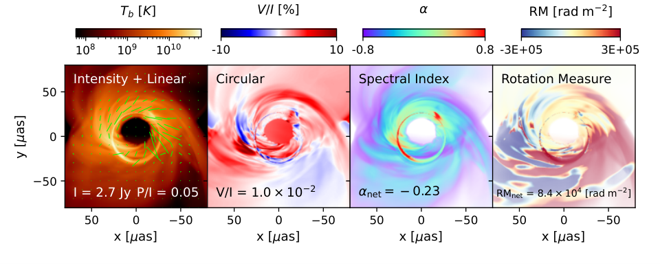
In this paper, we review how properties of the spacetime and the plasma become imprinted onto multifrequency polarimetric observables accessible to the EHT and ngEHT. In Figure 1, we plot a single GRMHD snapshot, ray-traced at 214 and 228 GHz with ipole (Mościbrodzka and Gammie 2018) and scaled to Sagittarius A*. This particular model is a MAD model with , , and a viewing angle of . So far, the EHT has produced total intensity maps for both M87∗ and Sgr A∗ and a linear polarization map of M87∗. The remaining maps have yet to be generated for EHT data, and will be explained in detail in this paper. In brief, circular polarization may arise from both Faraday conversion and intrinsically emitted synchrotron (Wardle and Homan 2003, e.g.,), and is especially sensitive to details of the underlying magnetic field geometry (Mościbrodzka et al. 2021; Ricarte et al. 2021; Tsunetoe et al. 2021) and plasma composition (Wardle et al. 1998; Anantua et al. 2020; Emami et al. 2021). Meanwhile, the spectral index is the logarithmic derivative of the flux or intensity with respect to frequency, , which helps break degeneracies between number density, temperature, and magnetic field strength (Bower et al. 2019; Ricarte et al. 2022). Finally, rotation measure is the derivative of the electric vector position angle (EVPA or ) with respect to observing wavelength squared , which encodes Faraday rotation. Since colder electrons Faraday rotate more efficiently, the RM offers a glimpse into a colder population of electrons, which may exist at large number densities but may be too cold to contribute significantly to the intensity (Mościbrodzka et al. 2017; Jiménez-Rosales and Dexter 2018; Ricarte et al. 2020). As discussed by the other contributions to this special issue, the ngEHT will enable access to this expanse of information with higher image dynamic range than currently published EHT results (increasing from to ), improved spatial resolution (decreasing from about 20 as to 10-15 as), and time-resolved images of the dynamical activity in both M87∗ and Sgr A∗ over hundreds-to-thousands of gravitational timescales. This will result in movies of both the accretion disks and relativistic jets near SMBHs, and here we discuss what physical information each of these maps carry.
2 Total Intensity and Spectral Index
In the millimeter, we observe Sgr A∗ and M87∗ near the peak of emission from synchrotron radiation, where the flow transitions from optically thick to optically thin. Here, the emissivity scales approximately as , where is the electron number density, is the magnetic field strength, and is the electron temperature (in units of the electron rest mass energy). Each of these quantities can vary by orders of magnitude among different models, and thus even the total flux is informative for jointly constraining these parameters. To match the total flux of a given system, the fluid in ideal GRMHD simulations can be rescaled via , , and , where is the internal energy and is a scalar. After doing so, both MAD and SANE simulations are capable of matching the total flux of EHT sources at a single frequency, as well as broad image characteristics such as the image size (Event Horizon Telescope Collaboration et al. 2019e; Akiyama et al. 2022e). However, this rescaling causes SANE simulations to typically have orders of magnitude larger number density than MADs, due to their intrinsically weaker magnetic fields and lower temperatures (Event Horizon Telescope Collaboration et al. 2021b; Akiyama et al. 2022e). Consequently, any additional observables sensitive these variables immediately help break degeneracies and distinguish models.
For example, the degeneracies between , , and can be partially resolved with the spectral index, . Spectral index is mainly sensitive to the optical depth as well as the temperature and magnetic field strength in the combination (to which the critical synchrotron frequency is dependent) (Pandya et al. 2016, e.g.,). Ricarte et al. 2022 show that GRMHD models span a wide range of spectral indices, and that SANE models typically exhibit more negative spectral indices than MADs at a fixed optical depth due to their lower temperatures.
In the ngEHT era, multi-frequency VLBI will enable not only spatially unresolved spectral index measurements, but also spectral index maps. Since the most important parameters (, , and ) all decline with radius, spectral index maps should generically grow more negative as radius increases. Equivalently, the image becomes smaller as the frequency grows larger (Blandford and Königl 1979, e.g.,). One example from Ricarte et al. 2022 is shown in Figure 2, a MAD simulation of Sgr A∗ with , , and a non-thermal “kappa” electron distribution function with (Vasyliunas 1968; Xiao 2006), inclined at . The true spectral index map across 214 to 228 GHz is shown in the top central panel, while a one-zone analytic prediction is shown in the top right, using a eDF combined with the plasma variables computed in the bottom row. To obtain the analytic prediction, each pixel is treated as a one-zone model using plasma properties computed via an emissivity-weighted average along the geodesic. In this simulation, both and decline with radius, but stays in a relatively narrow range. Thus, the decline of with radius can be attributed to a decline in and . Models also exhibit a generic spike in in the photon ring, whose geodesics plunge into regions with strong magnetic fields and acquire a larger optical depth due to their longer path lengths in the emitting region.


3 Linear Polarization

A uniform parcel of synchrotron emitting optically thin plasma intrinsically produces a linear polarization fraction of , with an orientation perpendicular to the local magnetic field projected onto the sky (Rybicki and Lightman 1986, e.g.,). The observed orientation of this linear polarization gets modified by two effects: achromatic effects of propagation through the curved space-time, and chromatic “Faraday” effects of propagation through a magnetized plasma (Himwich et al. 2020; Narayan et al. 2021; Gelles et al. 2021; Palumbo and Wong 2022, recent theoretical investigations in a the vicinity of a black hole include ). Both rotate and potentially scramble the electric vector position angle (EVPA, or ). Thus, resolved images of linear polarization can inform us about the magnetic field geometry, the magnitude of Faraday effects, and potentially the space-time itself. In Figure 3, we plot the linear polarization pattern of a ring of emission moving clockwise on the sky around a Schwarzschild black hole using the model of Narayan et al. 2021. Here, only the direct () sub-image is included. The ring is located at a radius of and has a Gaussian width of . The angular momentum vector of the ring projected onto the sky has a position angle of East of North and is viewed at an inclination of , consistent with that of M87∗ (Walker et al. 2018). In the toroidal and radial field cases, the resulting linear polarization pattern is simply perpendicular to the magnetic fields projected onto the line-of-sight. In the idealized vertical case, the EVPA pattern becomes more sensitive to the direction of the fluid’s motion (Event Horizon Telescope Collaboration et al. 2021b).
EHT studies have identified the linear polarization fraction (on both resolved and unresolved scales) as well as the morphology of polarization ticks as important observables for theoretical interpretation. This “twistiness” can be quantified by the quantity , the azimuthally symmetric component of a Fourier decomposition of the polarization pattern (Palumbo et al. 2020). M87∗ and Sgr A∗ both exhibit much lower linear polarization fractions than the ideal value of 70% for a uniform parcel of emitting plasma (Goddi et al. 2021), as do other low luminosity AGN (Lister et al. 2018, e.g.,). Event Horizon Telescope Collaboration et al. 2021b found that such low polarization fractions could be obtained by significant Faraday rotation scrambling. Combining resolved linear polarization information with an upper limit on circular polarization, Event Horizon Telescope Collaboration et al. 2021b found that MAD models were favored over their SANE counterparts for M87∗, which could not be concluded based on total intensity alone. Fundamentally, this can be attributed to linear polarization’s sensitivity to the geometry of the magnetic field, as well as Faraday rotation’s sensitivity to cooler electrons that may otherwise be invisible. MAD models tend to have more ordered fields with stronger poloidal components, which produces twistier polarization patterns. Meanwhile, SANE models tend to require orders of magnitude larger mass density to compensate for their intrinsically weaker magnetic fields and lower temperatures, resulting in much greater Faraday depths. In retrograde systems, images can exhibit flips in the sign of that correspond to a flip in the angular velocity of inflowing streams due to frame dragging (Ricarte et al. 2022).
Sgr A∗ also exhibits interesting time variability in linear polarization, especially during flares, which are accompanied by large polarization fractions, swings in polarization angle, and “- loops” on the timescale of hours (Marrone et al. 2006; Trippe et al. 2007; Zamaninasab et al. 2011; GRAVITY Collaboration et al. 2018; Wielgus et al. 2022). These can be interpreted as the motion of hotspots or other structures as they light up different parts of the magnetic field structure during their orbit (Broderick and Loeb 2005; GRAVITY Collaboration et al. 2020; Gelles et al. 2021; Vos et al. 2022). The hotspots themselves may originate from “flux eruption events” and magnetic reconnection that occur naturally in MAD accretion flows (Ripperda et al. 2020; Dexter et al. 2020; Chatterjee and Narayan 2022). Thus, time variability of linear polarization offers unique insights into the magnetic field structure and direction of orbital motion that could potentially be linked to the inclination and spin of Sgr A∗. The GRAVITY Collaboration has detected centroid motion coincident with a flare (GRAVITY Collaboration et al. 2018; GRAVITY Collaboration et al. 2020). Spatially resolved movies created by the ngEHT would help test the hotspot interpretation, motivating high-cadence monitoring of this source.
4 Rotation Measure
In an ionic plasma, circularly polarized waves of opposite handedness propagate at different speeds, resulting in a circular birefringence effect known as Faraday rotation. The EVPA of propagating emission rotates an amount sensitive to the density, temperature, and line-of-sight magnetic field. As examined in several studies, internal Faraday rotation is important for depolarizing and scrambling images of GRMHD models of black hole accretion flows (Mościbrodzka et al. 2017; Jiménez-Rosales and Dexter 2018; Ricarte et al. 2020; Event Horizon Telescope Collaboration et al. 2021b). The magnitude of Faraday rotation has a wavelength-squared dependence, thus it is useful observationally to define the rotation measure , which offers insights into physical parameters of the Faraday rotating plasma. For a linearly polarized emitter entirely behind a uniform of Faraday screen, the RM is related to the properties of the screen via
| (1) |
where is the electron number density, is the component of the magnetic field parallel to the photon wave-vector, and is a correction term suppressing Faraday rotation at relativistic temperatures (Gardner and Whiteoak 1966). For relativistic plasmas, , while asymptotes to 1 as . Here , is the Boltzmann constant, is the electron temperature, is the electron rest mass, and is the speed of light (Jones and Odell 1977). In GRMHD models, the plasma responsible for synchrotron emission is sometimes completely separate from the plasma responsible for Faraday rotation. For example, some large SANE models exhibit a cold Faraday rotating midplane sandwiched between emission from their hot jet sheaths (Ricarte et al. 2020). Hence, rotation measure and linear polarization can offer a view into electron populations that may otherwise be undetectable from total intensity alone.

At the time of writing, narrow observing bandwidths inhibit our ability to create spatially resolved rotation measure maps, but spatially unresolved RM measurements at millimeter wavelengths exist for Sgr A*, the core of M87∗, and several other LLAGN (Marrone et al. 2007; Plambeck et al. 2014; Kuo et al. 2014; Bower et al. 2018; Park et al. 2019; Marti-Vidal and Muller 2019, e.g.,). Note also that rotation measure from AGN generally increases with increasing frequency (Kravchenko et al. 2017, e.g.,) and can reach values of the order of (Martí-Vidal et al. 2015) due to the opacity effect probing regions close to the central engine at the ngEHT frequencies. Without spatial resolution, unresolved rotation measure measurements are difficult to interpret because the assumptions underlying Equation 1 are not believed to generally hold. In GRMHD models, Faraday rotation occurs co-spatially with the plasma, can vary by orders of magnitude in different locations, and can also flip sign across the image due to turbulence (Ricarte et al. 2020). As a result, unresolved EVPA measurements may exhibit significant temporal variation and not strictly follow a law. Figure 4 plots a rotation measure map of a MAD GRMHD model of M87∗, with the spatially unresolved RM written at the bottom of each panel. This turbulence can explain the intra-week time variability of the RM observed for M87∗ (Goddi et al. 2021). On the other hand, Sgr A∗ has exhibited a constant sign of RM for decades, suggesting the existence of a more stable (but still variable) foreground Faraday screen (Bower et al. 2018). Spatially resolved rotation measure maps could help disentangle the Faraday screen and give insights into both the turbulence of the accretion flow and the magnetic field structure of jets. This may be of increased importance, since EHT observations of Sgr A∗ indicate that GRMHD models are too variable (Akiyama et al. 2022e).
5 Circular Polarization
 |
Circular polarization, Stokes V, can be generated both intrinsically through synchrotron emission or through Faraday conversion, which exchanges linear and circular polarization states (Wardle and Homan 2003, e.g.,). Circular polarization fractions are much lower than their linear counterparts for both Sgr A∗ () and M87∗ (), making it more challenging to study than linear polarization. In addition, the circular feed basis used for EHT sites makes it more challenging to construct circularly polarized images. However, Stokes V has the potential to encode not only the magnetic field direction and geometry, but also the plasma composition.
Unlike the near unity linear polarization fractions produced by a uniform parcel of plasma, intrinsically emitted Stokes V is typically produced at the 1% level for plasma parameters appropriate for M87∗ or Sgr A∗. The sign of intrinsically emitted circular polarization generated encodes the sign of the magnetic field along the line of sight, following the right hand rule. The second is Faraday conversion, which exchanges linear and circular polarization states. The sign of circular polarization generated by conversion depends on the relative orientation of the EVPA with respect to the local magnetic field. Specifically, Stokes V generated by conversion inherits the sign of Stokes U, defined in the local plasma frame. Thus, Stokes V from Faraday conversion is sensitive to the line of sight “twist” in the magnetic field as well as any Faraday rotation affecting the EVPA of the linear polarization that gets converted. Interestingly, Faraday conversion has no effect in a unidirectional magnetic field lacking Faraday rotation.
Both intrinsic emission and Faraday conversion are believed to be important for generating circular polarization on event horizon scales (Mościbrodzka et al. 2021; Ricarte et al. 2021; Tsunetoe et al. 2021). For Faraday conversion, both the line of sight twist in the magnetic field and Faraday rotation are important for determining the orientation of the linear polarization that is converted into circular. Small amounts of Faraday rotation can affect the relative alignment between linear polarization and the converting magnetic field. Large amounts of Faraday rotation can lead to depolarization by randomizing the sign of Stokes U that is converted into Stokes V.
Figure 5depicts a cartoon of a typical helical field geometry as well as the circular polarization produced by a model that exhibits this structure (Ricarte et al. 2021, reproduced from). In the left panel, the background colors depict the line of sight direction of the magnetic field, viewed edge-on. In the time averaged image of viewed at 90∘, This structure produces a “four quadrants” pattern at large scales, in the time averaged image of viewed at 90∘, where on large scales Stokes V originates from intrinsic emission (Tsunetoe et al. 2021, see also). Another interesting feature that arises due to a generic helical field geometry is the successive sign flipping of sub-images in the photon ring (Mościbrodzka et al. 2021, also discussed in), which can be explained by Faraday conversion and parallel transport in a generic helical field geometry viewed face-on (Ricarte et al. 2021). In this particular model, the spatially unresolved Stokes V is surprisingly dominated by this sign-flipped photon ring.
Finally, circular polarization is strongly affected by plasma composition, and can potentially be used to distinguish pair plasmas from ionic plasmas (Wardle et al. 1998, e.g.,). Most models used to study EHT images have contained only ionic plasma. Electron-positron pairs can also be naturally produced on event horizon scales, but their abundance is highly theoretically uncertain. In a pair plasma, intrinsic circularly polarized emission and Faraday rotation both vanish, but Faraday conversion persists. Intuitively, a pair plasma with equal parts positively and negatively charged particles should not gyrate in a preferred direction. This can cause dramatic differences in images of circular polarization, and potentially also those of linear polarization (Anantua et al. 2020; Emami et al. 2021).
6 Scattering
A major challenge for studies of Sgr A* with the EHT and ngEHT is interstellar scattering by dilute plasma in the ionized interstellar medium. In particular, the line of sight to Sgr A* is heavily scattered by plasma in the spiral arms of the Milky Way (Bower et al. 2014), resulting in angular broadening that is approximately three orders of magnitude larger than median values for lines of sight at higher galactic latitudes. The effects of scattering are two-fold: 1) small-scale modes in the scattering material result in diffractive “blurring,” described by a convolution with an anisotropic kernel, and 2) large-scale modes in the scattering material result in refractive “substructure,” described by additive image noise with a slowly falling power spectrum. For detailed discussion of the scattering of Sgr A*, see Psaltis et al. 2018; Johnson et al. 2018; Johnson et al. 2021.
While the scattering severely affects images of Sgr A*, many polarimetric properties of the images are comparatively immune because the scattering is not significantly birefringent. For example, in the case of purely diffractive scattering, the image-integrated fractional polarization is independent of scattering. More generally, the interferometric fractional polarization is independent of diffractive scattering because convolution is multiplicative in the visibility domain and is identical for all Stokes parameters, thereby canceling in the quotient.
Figure 6shows an example GRMHD snapshot before and after scattering. While the images look substantially different, key polarimetric observables such as the mode, which is highly constraining for GRMHD models Event Horizon Telescope Collaboration et al. 2021b and carries information about black hole spin Palumbo et al. 2020, are almost unaffected by scattering. Likewise, certain interferometric observables, such as the interferometric fractional polarization, are only mildly affected by scattering (see Figure 7). For additional discussion of how the deterministic frequency dependence of scattering can be used for scattering mitigation on images, see Johnson 2016; for discussion of how the lack of birefringence can be used to study the relative power spectra in different polarization modes, see Ni et al. (in prep).


7 Studying Polarimetry with Interferometry
Thus far, the discussion has focused on the polarimetric properties of simulated black hole images or images reconstructed from interferometric visibilities. In practice, since the measured visibilities are actually samples of the Fourier transform, image reconstruction can introduce significant systematic uncertainties. Reconstruction methods must find images consistent with incomplete and noisy information in Fourier space, to which there can be multiple families of solutions. Images cannot be constructed at all without sufficient coverage (or strict image priors). Thus, it can be useful to study signals in their native visibility space.

The visibility-domain response of polarimetric observables has some key differences from that of total intensity. For instance, the visibility amplitude for total intensity is guaranteed to be maximal for the zero baseline because the image is positive. However, because the Stokes parameters , , and are not constrained to be positive, their visibility functions may not be maximal on the zero baseline. This simple property can be used to make powerful inferences from sparse measurements (e.g., from the EHT or RadioAstron). For instance, a single measurement of would demonstrate that the image does not have uniform sign of circular polarization. Likewise, if , where , then the linear polarization field must have variations in direction. This test can be performed with as few as two stations, but each must have dual polarization receivers.
A more significant difference between the total intensity and polarization is that the linear polarization can have changes in both amplitude and direction, allowing it to have significant image substructure relative to the intensity image. In the visibility domain, this substructure translates to a relative increase in the power on long baselines in polarization versus total intensity. In the limit of a heavily resolved source, the polarimetric signal may exceed that of the total intensity, even for a source with a low fractional polarization!
This can be quantified using the interferometric fractional polarization, . This complex quantity corresponds to the unresolved fractional polarization on a zero baseline, , where the “tot” subscript denotes an image-integrated quantity. However, unlike the image fractional polarization, can exceed unity on long baselines. This was found out from ground-based observations of for Sgr A* (Johnson et al. 2015) as well as within the RadioAstron Space VLBI survey of AGN (Kovalev et al. 2020). These observations had one common feature: a very high angular resolution corresponding to several G spatial scales. In general, for a heavily resolved source with polarized substructure, we expect to generically grow with increasing baseline length.
From a calibration perspective, the interferometric fractional polarization has the benefit of properties analogous to VLBI closure quantities, since the source of rapidly varying gains at VLBI sites (e.g., changing atmospheric delay and reference frequency errors) are equivalent for both polarization feeds. In addition, the interferometric fractional polarization is resilient to the effects of interstellar scattering, which is likewise not significantly birefringent (see Figure 7). Finally, is a useful observable to measure the relative coherence of the polarization field. For a perfectly uniform polarization field, will be independent of baseline length. However, for a disordered polarization field, will grow roughly as , as the observations resolve the structure in total intensity without resolving the structure in polarization.
In Figure 8, we plot total intensity and linear polarization maps of two models of M87∗ with very different polarization characteristics. The top model is a MAD simulation with and , which exhibits an ordered polarization pattern due to ordered magnetic fields and little Faraday rotation. Meanwhile, the bottom model is a SANE simulation with and . As mentioned in section 4, SANE simulations tend to have much larger Faraday depths than MADs, causing this model’s linear polarization to be much more disordered. The pixel-to-pixel intensity weighted Faraday depth is written at the bottom of each panel.
These characteristics are reflected in their Fourier space maps of and , shown in the second and third columns, which can be directly sampled using an interferometer. Here, and , where denotes a Fourier transform. For the MAD model, and both rise dramatically with radius in Fourier space. rises because the linear polarization is higher on resolved scales than a spatially unresolved measurement would suggest. The rotational symmetry of the polarization pattern causes substantial cancellation of polarization without spatial resolution. also rises for this reason, and also because exhibits nulls in Fourier space that do not necessarily coincide with the nulls in . Meanwhile, the disordered SANE simulation exhibits a mottled pattern in with a characteristic length scale corresponding to the size of the image. These phenomena should not change much qualitatively as a function of wavelength in the sub-millimeter.
The previous discussion has focused on the relationship between expected image features and their appearance in the (Fourier-conjugate) interferometric visibility domain. However, a crucial consideration is how to study frequency-dependent effects, such as spectral index and rotation measure, using interferometry. Because the fringe spacing , interferometric measurements across multiple frequencies necessarily mix the effects of a changing dimensionless baseline with those of a changing image.
Specifically, the interferometric response on a physical vector baseline at an observing frequency is
| (2) | ||||
| (3) |
The first term in the square brackets accounts for the frequency dependence of the image, while the second accounts for the changing dimensionless baseline with frequency. For the first term, an image with spectral index has , while the effects of RM give . Roughly speaking, we expect that the relative dominance or subdominance of spectral index versus RM are independent of baseline length, so the relative effects on long baselines are likely similar to those for unresolved measurements of a source. For instance, the effects of rotation measure for observations of Sgr A∗ at millimeter wavelengths are likely to vastly dominate the effects of spectral index. Sgr A∗ has (Wielgus et al. 2022) but (Goddi et al. 2021). The second term gives a relative contribution that increases as the image is increasingly resolved. It becomes significant when the spanned frequencies change the baseline length by the inverse field-of-view, .
8 Discussion and Conclusion
The EHT and upcoming ngEHT enable us to probe accreting supermassive black holes via a variety of multi-frequency polarimetric observables. In this contribution, we have discussed the many ways in which the physical properties of underlying accretion flow are mapped onto these observables. Total intensity and spectral index encode the density, temperature, and magnetic field strength of emitting plasma in different regions. Linear polarization encodes the geometry of the magnetic field, and its depolarization via Faraday rotation offers an observational probe into otherwise invisible cool electrons. Rotation measure maps probe this cooler Faraday rotating electron population directly, and can probe the magnetic field direction, which can reveal turbulent structures. Finally, circular polarization encodes both overall geometry and direction of the magnetic field via emission, Faraday rotation, and Faraday conversion. We have discussed that even if imaging proves prohibitively challenging for some datasets, constraining information exists already in visibility space. For some models, low polarization fractions in spatially unresolved measurements hide large polarization fractions in spatially resolved measurements. In the ngEHT era, we will have access to not only single snapshots, but also movies, with a much larger dynamic range in intensity than is presently possible with the EHT. Multiple snapshots will also enable cleaner theoretical connections via time averaging (Gold et al. 2017; Pushkarev et al. 2022, e.g.,). This will enable an unprecedented deluge of data about the nearest SMBHs that will help us understand their accretion and feedback processes.
9 Acknowledgments
We thank the National Science Foundation (AST-1716536, AST-1935980, AST-2034306, AST-1816420, and OISE-1743747) for financial support of this work. YYK was supported by the Russian Science Foundation grant 21-12-00241. This work was supported in part by the Black Hole Initiative, which is funded by grants from the John Templeton Foundation and the Gordon and Betty Moore Foundation to Harvard University. The opinions expressed in this publication are those of the author(s) and do not necessarily reflect the views of the Moore or Templeton Foundations.
References
- Event Horizon Telescope Collaboration et al. (2019a) Event Horizon Telescope Collaboration.; Akiyama, K.; Alberdi, A.; Alef, W.; Asada, K.; Azulay, R.; Baczko, A.K.; Ball, D.; Baloković, M.; Barrett, J.; et al. First M87 Event Horizon Telescope Results. I. The Shadow of the Supermassive Black Hole. ApJ 2019, 875, L1, [arXiv:astro-ph.GA/1906.11238]. https://doi.org/10.3847/2041-8213/ab0ec7.
- Event Horizon Telescope Collaboration et al. (2019b) Event Horizon Telescope Collaboration.; Akiyama, K.; Alberdi, A.; Alef, W.; Asada, K.; Azulay, R.; Baczko, A.K.; Ball, D.; Baloković, M.; Barrett, J.; et al. First M87 Event Horizon Telescope Results. II. Array and Instrumentation. ApJ 2019, 875, L2, [arXiv:astro-ph.IM/1906.11239]. https://doi.org/10.3847/2041-8213/ab0c96.
- Event Horizon Telescope Collaboration et al. (2019c) Event Horizon Telescope Collaboration.; Akiyama, K.; Alberdi, A.; Alef, W.; Asada, K.; Azulay, R.; Baczko, A.K.; Ball, D.; Baloković, M.; Barrett, J.; et al. First M87 Event Horizon Telescope Results. III. Data Processing and Calibration. ApJ 2019, 875, L3, [arXiv:astro-ph.GA/1906.11240]. https://doi.org/10.3847/2041-8213/ab0c57.
- Event Horizon Telescope Collaboration et al. (2019d) Event Horizon Telescope Collaboration.; Akiyama, K.; Alberdi, A.; Alef, W.; Asada, K.; Azulay, R.; Baczko, A.K.; Ball, D.; Baloković, M.; Barrett, J.; et al. First M87 Event Horizon Telescope Results. IV. Imaging the Central Supermassive Black Hole. ApJ 2019, 875, L4, [arXiv:astro-ph.GA/1906.11241]. https://doi.org/10.3847/2041-8213/ab0e85.
- Event Horizon Telescope Collaboration et al. (2019e) Event Horizon Telescope Collaboration.; Akiyama, K.; Alberdi, A.; Alef, W.; Asada, K.; Azulay, R.; Baczko, A.K.; Ball, D.; Baloković, M.; Barrett, J.; et al. First M87 Event Horizon Telescope Results. V. Physical Origin of the Asymmetric Ring. ApJ 2019, 875, L5, [arXiv:astro-ph.GA/1906.11242]. https://doi.org/10.3847/2041-8213/ab0f43.
- Event Horizon Telescope Collaboration et al. (2019f) Event Horizon Telescope Collaboration.; Akiyama, K.; Alberdi, A.; Alef, W.; Asada, K.; Azulay, R.; Baczko, A.K.; Ball, D.; Baloković, M.; Barrett, J.; et al. First M87 Event Horizon Telescope Results. VI. The Shadow and Mass of the Central Black Hole. ApJ 2019, 875, L6, [arXiv:astro-ph.GA/1906.11243]. https://doi.org/10.3847/2041-8213/ab1141.
- Event Horizon Telescope Collaboration et al. (2021a) Event Horizon Telescope Collaboration.; Akiyama, K.; Algaba, J.C.; Alberdi, A.; Alef, W.; Anantua, R.; Asada, K.; Azulay, R.; Baczko, A.K.; Ball, D.; et al. First M87 Event Horizon Telescope Results. VII. Polarization of the Ring. ApJ 2021, 910, L12, [arXiv:astro-ph.HE/2105.01169]. https://doi.org/10.3847/2041-8213/abe71d.
- Event Horizon Telescope Collaboration et al. (2021b) Event Horizon Telescope Collaboration.; Akiyama, K.; Algaba, J.C.; Alberdi, A.; Alef, W.; Anantua, R.; Asada, K.; Azulay, R.; Baczko, A.K.; Ball, D.; et al. First M87 Event Horizon Telescope Results. VIII. Magnetic Field Structure near The Event Horizon. ApJ 2021, 910, L13, [arXiv:astro-ph.HE/2105.01173]. https://doi.org/10.3847/2041-8213/abe4de.
- Akiyama et al. (2022a) Akiyama, K.; Alberdi, A.; Alef, W.; Algaba, J.C.; Anantua, R.; Asada, K.; Azulay, R.; Bach, U.; Baczko, A.K.; Ball, D.; et al. First Sagittarius A* Event Horizon Telescope Results. I. The Shadow of the Supermassive Black Hole in the Center of the Milky Way. ApJ 2022, 930, L12. https://doi.org/10.3847/2041-8213/ac6674.
- Akiyama et al. (2022b) Akiyama, K.; Alberdi, A.; Alef, W.; Algaba, J.C.; Anantua, R.; Asada, K.; Azulay, R.; Bach, U.; Baczko, A.K.; Ball, D.; et al. First Sagittarius A* Event Horizon Telescope Results. II. EHT and Multiwavelength Observations, Data Processing, and Calibration. ApJ 2022, 930, L13. https://doi.org/10.3847/2041-8213/ac6675.
- Akiyama et al. (2022c) Akiyama, K.; Alberdi, A.; Alef, W.; Algaba, J.C.; Anantua, R.; Asada, K.; Azulay, R.; Bach, U.; Baczko, A.K.; Ball, D.; et al. First Sagittarius A* Event Horizon Telescope Results. III. Imaging of the Galactic Center Supermassive Black Hole. ApJ 2022, 930, L14. https://doi.org/10.3847/2041-8213/ac6429.
- Akiyama et al. (2022d) Akiyama, K.; Alberdi, A.; Alef, W.; Algaba, J.C.; Anantua, R.; Asada, K.; Azulay, R.; Bach, U.; Baczko, A.K.; Ball, D.; et al. First Sagittarius A* Event Horizon Telescope Results. IV. Variability, Morphology, and Black Hole Mass. ApJ 2022, 930, L15. https://doi.org/10.3847/2041-8213/ac6736.
- Akiyama et al. (2022e) Akiyama, K.; Alberdi, A.; Alef, W.; Algaba, J.C.; Anantua, R.; Asada, K.; Azulay, R.; Bach, U.; Baczko, A.K.; Ball, D.; et al. First Sagittarius A* Event Horizon Telescope Results. V. Testing Astrophysical Models of the Galactic Center Black Hole. ApJ 2022, 930, L16. https://doi.org/10.3847/2041-8213/ac6672.
- Akiyama et al. (2022f) Akiyama, K.; Alberdi, A.; Alef, W.; Algaba, J.C.; Anantua, R.; Asada, K.; Azulay, R.; Bach, U.; Baczko, A.K.; Ball, D.; et al. First Sagittarius A* Event Horizon Telescope Results. VI. Testing the Black Hole Metric. ApJ 2022, 930, L17. https://doi.org/10.3847/2041-8213/ac6756.
- Ricarte et al. (2022) Ricarte, A.; et al. in prep. 2022.
- Bisnovatyi-Kogan and Ruzmaikin (1974) Bisnovatyi-Kogan, G.S.; Ruzmaikin, A.A. The Accretion of Matter by a Collapsing Star in the Presence of a Magnetic Field. Ap&SS 1974, 28, 45–59. https://doi.org/10.1007/BF00642237.
- Igumenshchev et al. (2003) Igumenshchev, I.V.; Narayan, R.; Abramowicz, M.A. Three-dimensional Magnetohydrodynamic Simulations of Radiatively Inefficient Accretion Flows. ApJ 2003, 592, 1042–1059, [arXiv:astro-ph/astro-ph/0301402]. https://doi.org/10.1086/375769.
- Narayan et al. (2003) Narayan, R.; Igumenshchev, I.V.; Abramowicz, M.A. Magnetically Arrested Disk: an Energetically Efficient Accretion Flow. PASJ 2003, 55, L69–L72, [arXiv:astro-ph/astro-ph/0305029]. https://doi.org/10.1093/pasj/55.6.L69.
- Narayan et al. (2012) Narayan, R.; SÄ dowski, A.; Penna, R.F.; Kulkarni, A.K. GRMHD simulations of magnetized advection-dominated accretion on a non-spinning black hole: role of outflows. MNRAS 2012, 426, 3241–3259, [arXiv:astro-ph.HE/1206.1213]. https://doi.org/10.1111/j.1365-2966.2012.22002.x.
- Sądowski et al. (2013) Sądowski, A.; Narayan, R.; Penna, R.; Zhu, Y. Energy, momentum and mass outflows and feedback from thick accretion discs around rotating black holes. MNRAS 2013, 436, 3856–3874, [arXiv:astro-ph.HE/1307.1143]. https://doi.org/10.1093/mnras/stt1881.
- Shapiro et al. (1976) Shapiro, S.L.; Lightman, A.P.; Eardley, D.M. A two-temperature accretion disk model for Cygnus X-1: structure and spectrum. ApJ 1976, 204, 187–199. https://doi.org/10.1086/154162.
- Rees et al. (1982) Rees, M.J.; Begelman, M.C.; Blandford, R.D.; Phinney, E.S. Ion-supported tori and the origin of radio jets. Nature 1982, 295, 17–21. https://doi.org/10.1038/295017a0.
- Narayan et al. (1995) Narayan, R.; Yi, I.; Mahadevan, R. Explaining the spectrum of Sagittarius A∗ with a model of an accreting black hole. Nature 1995, 374, 623–625. https://doi.org/10.1038/374623a0.
- Mościbrodzka et al. (2016) Mościbrodzka, M.; Falcke, H.; Shiokawa, H. General relativistic magnetohydrodynamical simulations of the jet in M 87. A&A 2016, 586, A38, [arXiv:astro-ph.HE/1510.07243]. https://doi.org/10.1051/0004-6361/201526630.
- Özel et al. (2000) Özel, F.; Psaltis, D.; Narayan, R. Hybrid Thermal-Nonthermal Synchrotron Emission from Hot Accretion Flows. ApJ 2000, 541, 234–249, [arXiv:astro-ph/astro-ph/0004195]. https://doi.org/10.1086/309396.
- Mao et al. (2017) Mao, S.A.; Dexter, J.; Quataert, E. The impact of non-thermal electrons on event horizon scale images and spectra of Sgr A*. MNRAS 2017, 466, 4307–4319, [arXiv:astro-ph.HE/1611.04601]. https://doi.org/10.1093/mnras/stw3324.
- Cruz-Osorio et al. (2022) Cruz-Osorio, A.; Fromm, C.M.; Mizuno, Y.; Nathanail, A.; Younsi, Z.; Porth, O.; Davelaar, J.; Falcke, H.; Kramer, M.; Rezzolla, L. State-of-the-art energetic and morphological modelling of the launching site of the M87 jet. Nature Astronomy 2022, 6, 103–108, [arXiv:astro-ph.HE/2111.02517]. https://doi.org/10.1038/s41550-021-01506-w.
- Fromm et al. (2022) Fromm, C.M.; Cruz-Osorio, A.; Mizuno, Y.; Nathanail, A.; Younsi, Z.; Porth, O.; Olivares, H.; Davelaar, J.; Falcke, H.; Kramer, M.; et al. Impact of non-thermal particles on the spectral and structural properties of M87. A&A 2022, 660, A107, [arXiv:astro-ph.HE/2111.02518]. https://doi.org/10.1051/0004-6361/202142295.
- Anantua et al. (2020) Anantua, R.; Emami, R.; Loeb, A.; Chael, A. Determining the Composition of Relativistic Jets from Polarization Maps. ApJ 2020, 896, 30, [arXiv:astro-ph.HE/1909.09230]. https://doi.org/10.3847/1538-4357/ab9103.
- Emami et al. (2021) Emami, R.; Anantua, R.; Chael, A.A.; Loeb, A. Positron Effects on Polarized Images and Spectra from Jet and Accretion Flow Models of M87* and Sgr A*. ApJ 2021, 923, 272, [arXiv:astro-ph.HE/2101.05327]. https://doi.org/10.3847/1538-4357/ac2950.
- Wong and Gammie (2022) Wong, G.N.; Gammie, C.F. Effects of Hydrogen vs. Helium on Electromagnetic Black Hole Observables. arXiv e-prints 2022, p. arXiv:2207.13705, [arXiv:astro-ph.HE/2207.13705].
- Fragile et al. (2007) Fragile, P.C.; Blaes, O.M.; Anninos, P.; Salmonson, J.D. Global General Relativistic Magnetohydrodynamic Simulation of a Tilted Black Hole Accretion Disk. ApJ 2007, 668, 417–429, [arXiv:astro-ph/0706.4303]. https://doi.org/10.1086/521092.
- Liska et al. (2021) Liska, M.; Hesp, C.; Tchekhovskoy, A.; Ingram, A.; van der Klis, M.; Markoff, S.B.; Van Moer, M. Disc tearing and Bardeen-Petterson alignment in GRMHD simulations of highly tilted thin accretion discs. MNRAS 2021, 507, 983–990, [arXiv:astro-ph.HE/1904.08428]. https://doi.org/10.1093/mnras/staa099.
- Mościbrodzka and Gammie (2018) Mościbrodzka, M.; Gammie, C.F. IPOLE - semi-analytic scheme for relativistic polarized radiative transport. MNRAS 2018, 475, 43–54, [arXiv:astro-ph.HE/1712.03057]. https://doi.org/10.1093/mnras/stx3162.
- Wardle and Homan (2003) Wardle, J.F.C.; Homan, D.C. Theoretical Models for Producing Circularly Polarized Radiation in Extragalactic Radio Sources. Ap&SS 2003, 288, 143–153, [arXiv:astro-ph/astro-ph/0305136]. https://doi.org/10.1023/B:ASTR.0000005001.80514.0c.
- Mościbrodzka et al. (2021) Mościbrodzka, M.; Janiuk, A.; De Laurentis, M. Unraveling circular polarimetric images of magnetically arrested accretion flows near event horizon of a black hole. MNRAS 2021, 508, 4282–4296, [arXiv:astro-ph.HE/2103.00267]. https://doi.org/10.1093/mnras/stab2790.
- Ricarte et al. (2021) Ricarte, A.; Qiu, R.; Narayan, R. Black hole magnetic fields and their imprint on circular polarization images. MNRAS 2021, 505, 523–539, [arXiv:astro-ph.HE/2104.11301]. https://doi.org/10.1093/mnras/stab1289.
- Tsunetoe et al. (2021) Tsunetoe, Y.; Mineshige, S.; Ohsuga, K.; Kawashima, T.; Akiyama, K. Polarization images of accretion flow around supermassive black holes: Imprints of toroidal field structure. PASJ 2021, 73, 912–928, [arXiv:astro-ph.HE/2012.05243]. https://doi.org/10.1093/pasj/psab054.
- Wardle et al. (1998) Wardle, J.F.C.; Homan, D.C.; Ojha, R.; Roberts, D.H. Electron-positron jets associated with the quasar 3C279. Nature 1998, 395, 457–461. https://doi.org/10.1038/26675.
- Bower et al. (2019) Bower, G.C.; Dexter, J.; Asada, K.; Brinkerink, C.D.; Falcke, H.; Ho, P.; Inoue, M.; Markoff, S.; Marrone, D.P.; Matsushita, S.; et al. ALMA Observations of the Terahertz Spectrum of Sagittarius A*. ApJ 2019, 881, L2, [arXiv:astro-ph.HE/1907.08319]. https://doi.org/10.3847/2041-8213/ab3397.
- Ricarte et al. (2022) Ricarte, A.; Gammie, C.; Narayan, R.; Prather, B.S. Probing Plasma Physics with Spectral Index Maps of Accreting Black Holes on Event Horizon Scales. arXiv e-prints 2022, p. arXiv:2202.02408, [arXiv:astro-ph.HE/2202.02408].
- Mościbrodzka et al. (2017) Mościbrodzka, M.; Dexter, J.; Davelaar, J.; Falcke, H. Faraday rotation in GRMHD simulations of the jet launching zone of M87. MNRAS 2017, 468, 2214–2221, [arXiv:astro-ph.HE/1703.02390]. https://doi.org/10.1093/mnras/stx587.
- Jiménez-Rosales and Dexter (2018) Jiménez-Rosales, A.; Dexter, J. The impact of Faraday effects on polarized black hole images of Sagittarius A*. MNRAS 2018, 478, 1875–1883, [arXiv:astro-ph.HE/1805.02652]. https://doi.org/10.1093/mnras/sty1210.
- Ricarte et al. (2020) Ricarte, A.; Prather, B.S.; Wong, G.N.; Narayan, R.; Gammie, C.; Johnson, M.D. Decomposing the internal faraday rotation of black hole accretion flows. MNRAS 2020, 498, 5468–5488, [arXiv:astro-ph.HE/2009.02369]. https://doi.org/10.1093/mnras/staa2692.
- Pandya et al. (2016) Pandya, A.; Zhang, Z.; Chandra, M.; Gammie, C.F. Polarized Synchrotron Emissivities and Absorptivities for Relativistic Thermal, Power-law, and Kappa Distribution Functions. ApJ 2016, 822, 34, [arXiv:astro-ph.HE/1602.08749]. https://doi.org/10.3847/0004-637X/822/1/34.
- Blandford and Königl (1979) Blandford, R.D.; Königl, A. Relativistic jets as compact radio sources. ApJ 1979, 232, 34–48. https://doi.org/10.1086/157262.
- Vasyliunas (1968) Vasyliunas, V.M. A survey of low-energy electrons in the evening sector of the magnetosphere with OGO 1 and OGO 3. J. Geophys. Res. 1968, 73, 2839–2884. https://doi.org/10.1029/JA073i009p02839.
- Xiao (2006) Xiao, F. Modelling energetic particles by a relativistic kappa-loss-cone distribution function in plasmas. Plasma Physics and Controlled Fusion 2006, 48, 203–213. https://doi.org/10.1088/0741-3335/48/2/003.
- Narayan et al. (2021) Narayan, R.; Palumbo, D.C.M.; Johnson, M.D.; Gelles, Z.; Himwich, E.; Chang, D.O.; Ricarte, A.; Dexter, J.; Gammie, C.F.; Chael, A.A.; et al. The Polarized Image of a Synchrotron-emitting Ring of Gas Orbiting a Black Hole. ApJ 2021, 912, 35, [arXiv:astro-ph.HE/2105.01804]. https://doi.org/10.3847/1538-4357/abf117.
- Rybicki and Lightman (1986) Rybicki, G.B.; Lightman, A.P. Radiative Processes in Astrophysics; 1986.
- Himwich et al. (2020) Himwich, E.; Johnson, M.D.; Lupsasca, A.; Strominger, A. Universal polarimetric signatures of the black hole photon ring. Phys. Rev. D 2020, 101, 084020, [arXiv:gr-qc/2001.08750]. https://doi.org/10.1103/PhysRevD.101.084020.
- Gelles et al. (2021) Gelles, Z.; Himwich, E.; Johnson, M.D.; Palumbo, D.C.M. Polarized image of equatorial emission in the Kerr geometry. Phys. Rev. D 2021, 104, 044060, [arXiv:gr-qc/2105.09440]. https://doi.org/10.1103/PhysRevD.104.044060.
- Palumbo and Wong (2022) Palumbo, D.C.M.; Wong, G.N. Photon Ring Symmetries in Simulated Linear Polarization Images of Messier 87*. ApJ 2022, 929, 49, [arXiv:astro-ph.HE/2203.00844]. https://doi.org/10.3847/1538-4357/ac59b4.
- Walker et al. (2018) Walker, R.C.; Hardee, P.E.; Davies, F.B.; Ly, C.; Junor, W. The Structure and Dynamics of the Subparsec Jet in M87 Based on 50 VLBA Observations over 17 Years at 43 GHz. ApJ 2018, 855, 128, [arXiv:astro-ph.HE/1802.06166]. https://doi.org/10.3847/1538-4357/aaafcc.
- Palumbo et al. (2020) Palumbo, D.C.M.; Wong, G.N.; Prather, B.S. Discriminating Accretion States via Rotational Symmetry in Simulated Polarimetric Images of M87. ApJ 2020, 894, 156, [arXiv:astro-ph.HE/2004.01751]. https://doi.org/10.3847/1538-4357/ab86ac.
- Goddi et al. (2021) Goddi, C.; Martí-Vidal, I.; Messias, H.; Bower, G.C.; Broderick, A.E.; Dexter, J.; Marrone, D.P.; Moscibrodzka, M.; Nagai, H.; Algaba, J.C.; et al. Polarimetric Properties of Event Horizon Telescope Targets from ALMA. ApJ 2021, 910, L14, [arXiv:astro-ph.GA/2105.02272]. https://doi.org/10.3847/2041-8213/abee6a.
- Lister et al. (2018) Lister, M.L.; Aller, M.F.; Aller, H.D.; Hodge, M.A.; Homan, D.C.; Kovalev, Y.Y.; Pushkarev, A.B.; Savolainen, T. MOJAVE. XV. VLBA 15 GHz Total Intensity and Polarization Maps of 437 Parsec-scale AGN Jets from 1996 to 2017. ApJS 2018, 234, 12, [arXiv:astro-ph.GA/1711.07802]. https://doi.org/10.3847/1538-4365/aa9c44.
- Ricarte et al. (2022) Ricarte, A.; Palumbo, D.C.M.; Narayan, R.; Roelofs, F.; Emami, R. Observational Signatures of Frame Dragging in Strong Gravity. arXiv e-prints 2022, p. arXiv:2211.01810, [arXiv:gr-qc/2211.01810].
- Marrone et al. (2006) Marrone, D.P.; Moran, J.M.; Zhao, J.H.; Rao, R. The Submillimeter Polarization of Sgr A*. In Proceedings of the Journal of Physics Conference Series, 2006, Vol. 54, Journal of Physics Conference Series, pp. 354–362, [arXiv:astro-ph/astro-ph/0607432]. https://doi.org/10.1088/1742-6596/54/1/056.
- Trippe et al. (2007) Trippe, S.; Paumard, T.; Ott, T.; Gillessen, S.; Eisenhauer, F.; Martins, F.; Genzel, R. A polarized infrared flare from Sagittarius A* and the signatures of orbiting plasma hotspots. MNRAS 2007, 375, 764–772, [arXiv:astro-ph/astro-ph/0611737]. https://doi.org/10.1111/j.1365-2966.2006.11338.x.
- Zamaninasab et al. (2011) Zamaninasab, M.; Eckart, A.; Dovčiak, M.; Karas, V.; Schödel, R.; Witzel, G.; Sabha, N.; García-Marín, M.; Kunneriath, D.; Mužić, K.; et al. Near-infrared polarimetry as a tool for testing properties of accreting supermassive black holes. MNRAS 2011, 413, 322–332, [arXiv:astro-ph.HE/1102.0775]. https://doi.org/10.1111/j.1365-2966.2010.18139.x.
- GRAVITY Collaboration et al. (2018) GRAVITY Collaboration.; Abuter, R.; Amorim, A.; Bauböck, M.; Berger, J.P.; Bonnet, H.; Brandner, W.; Clénet, Y.; Coudé Du Foresto, V.; de Zeeuw, P.T.; et al. Detection of orbital motions near the last stable circular orbit of the massive black hole SgrA*. A&A 2018, 618, L10, [arXiv:astro-ph.GA/1810.12641]. https://doi.org/10.1051/0004-6361/201834294.
- Wielgus et al. (2022) Wielgus, M.; Moscibrodzka, M.; Vos, J.; Gelles, Z.; Martí-Vidal, I.; Farah, J.; Marchili, N.; Goddi, C.; Messias, H. Orbital motion near Sagittarius A∗ . Constraints from polarimetric ALMA observations. A&A 2022, 665, L6, [arXiv:astro-ph.HE/2209.09926]. https://doi.org/10.1051/0004-6361/202244493.
- Broderick and Loeb (2005) Broderick, A.E.; Loeb, A. Imaging bright-spots in the accretion flow near the black hole horizon of Sgr A*. MNRAS 2005, 363, 353–362, [arXiv:astro-ph/astro-ph/0506433]. https://doi.org/10.1111/j.1365-2966.2005.09458.x.
- GRAVITY Collaboration et al. (2020) GRAVITY Collaboration.; Jiménez-Rosales, A.; Dexter, J.; Widmann, F.; Bauböck, M.; Abuter, R.; Amorim, A.; Berger, J.P.; Bonnet, H.; Brandner, W.; et al. Dynamically important magnetic fields near the event horizon of Sgr A*. A&A 2020, 643, A56, [arXiv:astro-ph.HE/2009.01859]. https://doi.org/10.1051/0004-6361/202038283.
- Vos et al. (2022) Vos, J.; Moscibrodzka, M.; Wielgus, M. Polarimetric signatures of hot spots in black hole accretion flows. arXiv e-prints 2022, p. arXiv:2209.09931, [arXiv:astro-ph.HE/2209.09931].
- Ripperda et al. (2020) Ripperda, B.; Bacchini, F.; Philippov, A.A. Magnetic Reconnection and Hot Spot Formation in Black Hole Accretion Disks. ApJ 2020, 900, 100, [arXiv:astro-ph.HE/2003.04330]. https://doi.org/10.3847/1538-4357/ababab.
- Dexter et al. (2020) Dexter, J.; Tchekhovskoy, A.; Jiménez-Rosales, A.; Ressler, S.M.; Bauböck, M.; Dallilar, Y.; de Zeeuw, P.T.; Eisenhauer, F.; von Fellenberg, S.; Gao, F.; et al. Sgr A* near-infrared flares from reconnection events in a magnetically arrested disc. MNRAS 2020, 497, 4999–5007, [arXiv:astro-ph.HE/2006.03657]. https://doi.org/10.1093/mnras/staa2288.
- Chatterjee and Narayan (2022) Chatterjee, K.; Narayan, R. Flux eruption events drive angular momentum transport in magnetically arrested accretion flows. arXiv e-prints 2022, p. arXiv:2210.08045, [arXiv:astro-ph.HE/2210.08045].
- GRAVITY Collaboration et al. (2020) GRAVITY Collaboration.; Bauböck, M.; Dexter, J.; Abuter, R.; Amorim, A.; Berger, J.P.; Bonnet, H.; Brandner, W.; Clénet, Y.; Coudé Du Foresto, V.; et al. Modeling the orbital motion of Sgr A*’s near-infrared flares. A&A 2020, 635, A143, [arXiv:astro-ph.HE/2002.08374]. https://doi.org/10.1051/0004-6361/201937233.
- Gardner and Whiteoak (1966) Gardner, F.F.; Whiteoak, J.B. The Polarization of Cosmic Radio Waves. ARA&A 1966, 4, 245. https://doi.org/10.1146/annurev.aa.04.090166.001333.
- Jones and Odell (1977) Jones, T.W.; Odell, S.L. Transfer of polarized radiation in self-absorbed synchrotron sources. I. Results for a homogeneous source. ApJ 1977, 214, 522–539. https://doi.org/10.1086/155278.
- Marrone et al. (2007) Marrone, D.P.; Moran, J.M.; Zhao, J.H.; Rao, R. An Unambiguous Detection of Faraday Rotation in Sagittarius A*. ApJ 2007, 654, L57–L60, [arXiv:astro-ph/astro-ph/0611791]. https://doi.org/10.1086/510850.
- Plambeck et al. (2014) Plambeck, R.L.; Bower, G.C.; Rao, R.; Marrone, D.P.; Jorstad, S.G.; Marscher, A.P.; Doeleman, S.S.; Fish, V.L.; Johnson, M.D. Probing the Parsec-scale Accretion Flow of 3C 84 with Millimeter Wavelength Polarimetry. ApJ 2014, 797, 66, [arXiv:astro-ph.GA/1410.5887]. https://doi.org/10.1088/0004-637X/797/1/66.
- Kuo et al. (2014) Kuo, C.Y.; Asada, K.; Rao, R.; Nakamura, M.; Algaba, J.C.; Liu, H.B.; Inoue, M.; Koch, P.M.; Ho, P.T.P.; Matsushita, S.; et al. Measuring Mass Accretion Rate onto the Supermassive Black Hole in M87 Using Faraday Rotation Measure with the Submillimeter Array. ApJ 2014, 783, L33, [arXiv:astro-ph.GA/1402.5238]. https://doi.org/10.1088/2041-8205/783/2/L33.
- Bower et al. (2018) Bower, G.C.; Broderick, A.; Dexter, J.; Doeleman, S.; Falcke, H.; Fish, V.; Johnson, M.D.; Marrone, D.P.; Moran, J.M.; Moscibrodzka, M.; et al. ALMA Polarimetry of Sgr A*: Probing the Accretion Flow from the Event Horizon to the Bondi Radius. ApJ 2018, 868, 101, [arXiv:astro-ph.HE/1810.07317]. https://doi.org/10.3847/1538-4357/aae983.
- Park et al. (2019) Park, J.; Hada, K.; Kino, M.; Nakamura, M.; Ro, H.; Trippe, S. Faraday Rotation in the Jet of M87 inside the Bondi Radius: Indication of Winds from Hot Accretion Flows Confining the Relativistic Jet. ApJ 2019, 871, 257, [arXiv:astro-ph.HE/1812.08386]. https://doi.org/10.3847/1538-4357/aaf9a9.
- Marti-Vidal and Muller (2019) Marti-Vidal, I.; Muller, S. Submillimeter polarization and variability of quasar PKS 1830-211. A&A 2019, 621, A18, [arXiv:astro-ph.GA/1810.11012]. https://doi.org/10.1051/0004-6361/201834036.
- Kravchenko et al. (2017) Kravchenko, E.V.; Kovalev, Y.Y.; Sokolovsky, K.V. Parsec-scale Faraday rotation and polarization of 20 active galactic nuclei jets. MNRAS 2017, 467, 83–101, [arXiv:astro-ph.HE/1701.00271]. https://doi.org/10.1093/mnras/stx021.
- Martí-Vidal et al. (2015) Martí-Vidal, I.; Muller, S.; Vlemmings, W.; Horellou, C.; Aalto, S. A strong magnetic field in the jet base of a supermassive black hole. Science 2015, 348, 311–314, [arXiv:astro-ph.HE/1604.01898]. https://doi.org/10.1126/science.aaa1784.
- Bower et al. (2018) Bower, G.C.; Broderick, A.; Dexter, J.; Doeleman, S.; Falcke, H.; Fish, V.; Johnson, M.D.; Marrone, D.P.; Moran, J.M.; Moscibrodzka, M.; et al. ALMA Polarimetry of Sgr A*: Probing the Accretion Flow from the Event Horizon to the Bondi Radius. ApJ 2018, 868, 101, [arXiv:astro-ph.HE/1810.07317]. https://doi.org/10.3847/1538-4357/aae983.
- Bower et al. (2014) Bower, G.C.; Deller, A.; Demorest, P.; Brunthaler, A.; Eatough, R.; Falcke, H.; Kramer, M.; Lee, K.J.; Spitler, L. The Angular Broadening of the Galactic Center Pulsar SGR J1745-29: A New Constraint on the Scattering Medium. ApJ 2014, 780, L2, [arXiv:astro-ph.GA/1309.4672]. https://doi.org/10.1088/2041-8205/780/1/L2.
- Psaltis et al. (2018) Psaltis, D.; Johnson, M.; Narayan, R.; Medeiros, L.; Blackburn, L.; Bower, G. A Model for Anisotropic Interstellar Scattering and its Application to Sgr A*. arXiv e-prints 2018, p. arXiv:1805.01242, [arXiv:astro-ph.HE/1805.01242].
- Johnson et al. (2018) Johnson, M.D.; Narayan, R.; Psaltis, D.; Blackburn, L.; Kovalev, Y.Y.; Gwinn, C.R.; Zhao, G.Y.; Bower, G.C.; Moran, J.M.; Kino, M.; et al. The Scattering and Intrinsic Structure of Sagittarius A* at Radio Wavelengths. ApJ 2018, 865, 104, [arXiv:astro-ph.GA/1808.08966]. https://doi.org/10.3847/1538-4357/aadcff.
- Johnson et al. (2021) Johnson, M.D.; Kovalev, Y.Y.; Lisakov, M.M.; Voitsik, P.A.; Gwinn, C.R.; Bruni, G. First Space-VLBI Observations of Sagittarius A*. ApJ 2021, 922, L28, [arXiv:astro-ph.GA/2111.06423]. https://doi.org/10.3847/2041-8213/ac3917.
- Palumbo et al. (2020) Palumbo, D.C.M.; Wong, G.N.; Prather, B.S. Discriminating Accretion States via Rotational Symmetry in Simulated Polarimetric Images of M87. ApJ 2020, 894, 156, [arXiv:astro-ph.HE/2004.01751]. https://doi.org/10.3847/1538-4357/ab86ac.
- Johnson (2016) Johnson, M.D. Stochastic Optics: A Scattering Mitigation Framework for Radio Interferometric Imaging. ApJ 2016, 833, 74, [arXiv:astro-ph.IM/1610.05326]. https://doi.org/10.3847/1538-4357/833/1/74.
- Johnson et al. (2015) Johnson, M.D.; Fish, V.L.; Doeleman, S.S.; Marrone, D.P.; Plambeck, R.L.; Wardle, J.F.C.; Akiyama, K.; Asada, K.; Beaudoin, C.; Blackburn, L.; et al. Resolved magnetic-field structure and variability near the event horizon of Sagittarius A*. Science 2015, 350, 1242–1245, [arXiv:astro-ph.HE/1512.01220]. https://doi.org/10.1126/science.aac7087.
- Kovalev et al. (2020) Kovalev, Y.Y.; Kardashev, N.S.; Sokolovsky, K.V.; Voitsik, P.A.; An, T.; Anderson, J.M.; Andrianov, A.S.; Avdeev, V.Y.; Bartel, N.; Bignall, H.E.; et al. Detection statistics of the RadioAstron AGN survey. Advances in Space Research 2020, 65, 705–711, [arXiv:astro-ph.GA/1909.00785]. https://doi.org/10.1016/j.asr.2019.08.035.
- Wielgus et al. (2022) Wielgus, M.; Marchili, N.; Martí-Vidal, I.; Keating, G.K.; Ramakrishnan, V.; Tiede, P.; Fomalont, E.; Issaoun, S.; Neilsen, J.; Nowak, M.A.; et al. Millimeter Light Curves of Sagittarius A* Observed during the 2017 Event Horizon Telescope Campaign. ApJ 2022, 930, L19, [arXiv:astro-ph.HE/2207.06829]. https://doi.org/10.3847/2041-8213/ac6428.
- Gold et al. (2017) Gold, R.; McKinney, J.C.; Johnson, M.D.; Doeleman, S.S. Probing the Magnetic Field Structure in Sgr A* on Black Hole Horizon Scales with Polarized Radiative Transfer Simulations. ApJ 2017, 837, 180, [arXiv:astro-ph.HE/1601.05550]. https://doi.org/10.3847/1538-4357/aa6193.
- Pushkarev et al. (2022) Pushkarev, A.B.; Aller, M.F.; Aller, H.D.; Homan, D.C.; Kovalev, Y.Y.; Lister, M.L.; Pashchenko, I.N.; Savolainen, T.; Zobnina, D. MOJAVE. XXI. Persistent Linear Polarization Structure in Parsec-scale AGN Jets. arXiv e-prints 2022, p. arXiv:2209.04842, [arXiv:astro-ph.HE/2209.04842].