AA YYYY
Galactic DynamosJournal: August 11, 2026DOI: 10.1146/((please add article doi))
Abstract
Spiral galaxies, including the Milky Way, have large-scale magnetic fields with significant energy densities. The dominant theory attributes these magnetic fields to a large-scale dynamo. We review the current status of dynamo theory and discuss various numerical simulations designed to explain either particular aspects of the problem or to reproduce galactic magnetic fields globally. Our main conclusions can be summarized as follows.
- •
Idealized direct numerical simulations produce mean magnetic fields, whose saturation energy density tends to decline with increasing magnetic Reynolds number. This is still an unsolved problem.
- •
Large-scale galactic magnetic fields of microgauss strengths can probably only be explained if helical magnetic fields of small or moderate length scales can rapidly be ejected or destroyed.
- •
Small-scale dynamos are important throughout a galaxy’s life, and probably provide strong seed fields at early stages.
- •
The circumgalactic medium (CGM) may play an important role in driving dynamo action at small and large length scales. These interactions between the galactic disk and the CGM may provide important insights into our understanding of galactic dynamos.
We expect future research in galactic dynamos to focus on the cosmological history of galaxies and the interaction with the CGM as means of replacing the idealized boundary conditions used in earlier work.
keywords
Spiral galaxies, Milky Way, large-scale magnetic fields, circumgalactic medium, magnetic Reynolds number1 INTRODUCTION
Many spiral galaxies have microgauss magnetic fields, so that their magnetic energy densities are comparable to the thermal, kinetic, and cosmic ray energy densities; see Ruzmaikin et al. 1988 for an early book on the subject, and Shukurov & Subramanian 2022 for a recent one; hereafter SS22. Similar magnetic field strengths have also been detected in galaxies at larger redshifts up to (Bernet et al. 2008, Mao et al. 2017).
Galactic magnetic fields often also show large-scale coherence. The first evidence for a global Galactic magnetic field comes from optical polarization (Hiltner 1949, Hall 1949). The existence of magnetic fields for other galaxies was later confirmed using synchrotron emission (Segalovitz et al. 1976), which showed systematic large-scale magnetic fields roughly in the direction of the galactic spiral arms. There has long been a debate about the origin of such magnetic fields: are they primordial or dynamo-generated, or perhaps a combination of the two? {marginnote}[] \entryDynamosconvert kinetic energy into magnetic energy Over the past few decades, attention has shifted from a primordial to a dynamo-generated origin. In the meantime, however, there have also been significant developments in dynamo theory, and global numerical simulations are now becoming more realistic. They tend to show that large-scale magnetic fields can be generated by a dynamo, but the amplitudes may be insufficient or the timescales for their generation too long for the simulations presented so far.
In this review, we focus on galactic dynamos and highlight the main developments since the time of the review of Beck et al. 1996. The broader problem of galactic magnetism that was addressed there will not be reviewed; we refer readers to the reviews by Beck 2001, Beck 2015a, Beck & Wielebinski 2013, and Han 2017, and the book by SS22. A review of astrophysical dynamos covering the era before 2005 is given by Brandenburg & Subramanian 2005a. The mathematics of small-scale turbulent dynamos is explained in the book by Zeldovich et al. 1990, and those in partially ionized plasmas are discussed by Xu & Lazarian 2021. We also recommend the reviews on ISM magnetic fields by Crutcher 2012, Hennebelle & Inutsuka 2019, and Pattle et al. 2022.
At the time of the review by Beck et al. 1996, there were results suggesting that the dynamo effect in mean-field theory is “catastrophically” quenched, i.e., it goes to zero as the magnetic Reynolds number () becomes large (Vainshtein & Cattaneo 1992, Cattaneo & Hughes 1996). {marginnote}[] \entryCatastrophic quenching means as , so it limits the large-scale field at large Specifically, the mean-field effect in question has been termed the effect, which quantifies the component of the mean electromagnetic force in the direction of the mean magnetic field. More generally, however, it means that the resulting mean (or large-scale) magnetic field cannot be generated at the expected amplitudes or time scales. This led to a major crisis in dynamo theory, questioning the possibility of an effect dynamo in the nonlinear regime beyond just infinitesimally weak kinematic dynamo-generated magnetic fields.
Although there are still unresolved questions in nonlinear dynamo theory today, there have also been major developments in this field: the importance of magnetic helicity fluxes has been recognized, mean-field dynamo coefficients can now be determined from simulations without the restrictions imposed by analytic techniques, and new dynamo mechanisms beyond just the effect have been explored. {marginnote}[] \entryMagnetic helicityVolume-integrated dot product of magnetic vector potential and magnetic field , At the same time, there has been significant progress in performing realistic three-dimensional (3-D) magnetohydrodynamic (MHD) simulations of galaxy formation, allowing a new theoretical view of the problem, where the circumgalactic medium (CGM) plays an integral part. All these developments motivate a new review on galactic dynamos.
[t]
2 Observational tracers of galactic magnetic fields
Dust extinction / emission polarization.
Elongated dust grains in the interstellar medium tend to align their minor axes with the mean magnetic field direction (Davis & Greenstein 1951). As a result, the light they emit in infrared wavelengths is polarized, with the polarization direction perpendicular to the mean direction of the magnetic field. Only recently has it been possible to trace extragalactic magnetic fields with this method (Lopez-Rodriguez et al. 2022, e.g.,the recent survey by).
Since starlight emission is unpolarized, we can also measure dust polarization in absorption against stellar sources. If the distances to the stars are known, it is possible to map the magnetic field at different locations along the line-of-sight (Tassis et al. 2018, e.g., the Polar-Areas Stellar-Imaging in Polarization High-Accuracy Experiment (PASIPHAE) survey,).
Synchrotron emission.
Ultra-relativistic cosmic ray particles emit polarized synchrotron radiation in radio wavelengths as they gyrate around the galactic magnetic field. Synchrotron emission, which yields the plane-of-the-sky magnetic field component in the warm/hot ISM, has been the tracer of choice for studying extragalactic magnetic fields (see, e.g., Beck 2012, for a review).
In general, linear polarization is measured through the Stokes parameters , , and . Then the observed polarization angle is calculated from the expression and the polarization fraction is .
Faraday Rotation.
When polarized radiation passes through an ionized magnetized medium, the plane of polarization is rotated by an angle , where is the observed wavelength and is in units of radians/. Here, is the distance to the source in pc, is the electron density in , and is the line-of-sight magnetic field of the medium in microgauss (Burn 1966, Brentjens & de Bruyn 2005). If we have an estimate of the electron density, then Faraday rotation can yield the line-of-sight magnetic field.
3 DYNAMOS
We begin by discussing historical and theoretical aspects of MHD and dynamos that are of particular importance in connection with the new developments in galactic dynamo research over the past few decades. The presence of a microphysical magnetic diffusivity plays here an important role. We begin with a historical perspective.
3.1 Historical remarks
In Section 14 we will discuss the observational signatures of dynamo models in detail. Here, we will only briefly mention some observational results that were significant for the development of dynamo models. For later reference, we provide here a short overview of the existing galactic magnetic field tracers in the text box on “Observational tracers of galactic magnetic fields”.
In the late 1970s, synchrotron radiation from external spiral galaxies began to reveal the presence of large-scale ordered magnetic fields broadly aligned with the galactic spiral pattern. At the time, an obvious possibility was that these magnetic fields were the result of winding up a pre-existing, large-scale field. This idea goes back to Piddington 1964 and Ôki et al. 1964, and is now commonly termed the primordial origin of the magnetic field. The resulting magnetic field is then expected to have the form of a bisymmetric spiral (BSS). The BSS form has a characteristic signature in the Faraday Rotation Measure (RM): when we observe an external galaxy almost, but not exactly, face-on, the line-of-sight magnetic field measured through RM probes the azimuthal component of the galactic field – see Figure 1 for a sketch. Using this technique, Tosa & Fujimoto 1978, who used a sketch similar to ours in Figure 1, found evidence for a BSS in M51. In an early review on galactic magnetic fields, Sofue et al. 1986 contrasted BSS with an axisymmetric spiral (ASS), expected from mean-field dynamo theory. Figure 1 also sketches the expected ASS signature.

However, a purely primordial origin of galactic magnetic fields implies that a tremendous amount of winding has occurred over the past due to the shear induced by the differential rotation of the galaxy. For example, in the solar neighborhood, the angular velocity of the Galaxy is , i.e., the rotation period is . This yields 70 revolutions in , so we would expect the magnetic field to be strongly wound up. Figure 2 gives a quantitative illustration of this wind-up process. It shows color scale images of together with field lines corresponding to the contours of the normal component of the magnetic vector potential, , so that the magnetic field in the plane is given by . To obtain the result shown in Figure 2, we solved the two-dimensional (2-D) induction equation, which corresponds to an advection–diffusion equation of the form
| (1) |
where . Here, we assumed that , where is the cylindrical position vector and is the angular velocity with , , and . This experiment demonstrates the extreme winding of the magnetic field. The turbulent magnetic diffusivity is here , corresponding to , which is three orders of magnitude below the canonical estimates (Brandenburg et al. 1993, SS22). We see about six windings at with a thirty-fold increase of . This amount of winding is not observed in any galaxy.
Mean-field dynamo theory was originally developed in the solar context (Steenbeck & Krause 1969) and can predict both axisymmetric and nonaxisymmetric magnetic fields (Baryshnikova et al. 1987). Parker 1971 was the first to show that the most easily excited axisymmetric large-scale magnetic fields in oblate bodies such as galaxies have an azimuthal component that is symmetric about the midplane, i.e., the fields have quadrupolar symmetry – in contrast to the dipolar symmetry that is often found in spherical bodies such as the Earth.

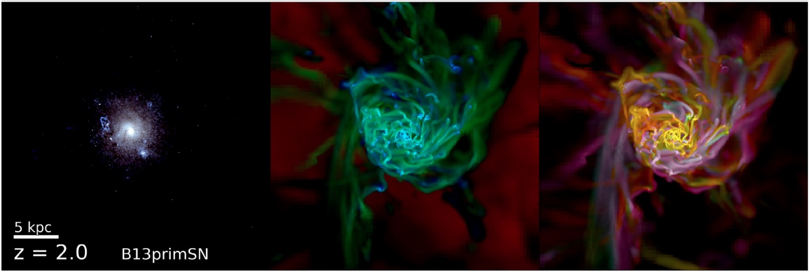
While dynamo theory can also produce BSS-type fields (Krasheninnikova et al. 1989), they are not the most easily excited modes (Elstner et al. 1990, Brandenburg et al. 1990), unless the turbulence is strongly anisotropic or the dynamo is controlled by strongly anisotropic flow structures (Moss et al. 1993). Today, the significance of primordial magnetic fields is still not resolved, and global 3-D numerical simulations suggest that both primordial and magnetic fields of astrophysical origin may be present in typical galaxies (e.g., Martin-Alvarez et al. 2021, see Figure 3).
3.2 The need for magnetic diffusivity: the example of steady flows
The evolution of the magnetic field is governed by the usual induction equation,
| (2) |
where is the velocity and is the current density with being the vacuum permeability. Equation 2 also includes an electric conductivity , because the mean-free path of the electrons in the interstellar medium (of the order of a few thousand astronomical units) is much smaller that the scales under study here. The magnetic resistivity is , and the microphysical magnetic diffusivity is then given by .
[t]
4 Characteristic nondimensional numbers
Fluid and magnetic Reynolds numbers and their ratio, the magnetic Prandtl number, are defined as
| (SB1) |
where is the root-mean square velocity, is the (microphysical) kinematic viscosity, is the (microphysical) magnetic diffusivity, and is the characteristic flow wavenumber. Note that the Reynolds numbers are sometimes based on the length scale, , which leads to about six times larger values. The present definition is commonly used in numerical simulations of turbulence. As a rule of thumb, the number of mesh points needed in a numerical simulation is similar to the value of the Reynolds number. In simulations with partial ionization, the ionization ratio enters as another nondimensional number.
Dynamos convert kinetic energy into magnetic energy through what is termed the dynamo instability. It occurs when the magnetic Reynolds number, , exceeds a certain critical value (for the definition of , see the text box titled “Characteristic nondimensional numbers”). Here, is the typical wavenumber of the flow. A rigorous definition of this instability is only possible for steady flows. Then an eigenvalue problem can be expressed through: , where is the eigenvalue and the eigenfunction. For steady, mass conserving, compressible flows, Moffatt & Proctor 1985 proved that dynamos (i.e., ) cannot exist for , i.e., in the strictly ideal case. This does not preclude dynamos in the astrophysically relevant limit , which are called fast dynamos (Soward 1987), but it is important to stress that the limit is quite different from the case .
The case is arguably pathological, because without resistivity, there is no Joule heating and the field line topology cannot change. This case is therefore of academic interest only, although it can be described using Euler potentials, and , such that , where and obey (Rosswog & Price 2007, e.g.,),
| (3) |
We see that in the special case of 2-D, this equation agrees with the advection–diffusion equation Equation 1, where and have been assumed. In this special case, it is possible to recover the induction equation in the presence of microphysical magnetic diffusion.
Dynamos have not been found in this formulation – even for 3-D turbulent or other flows that allow for dynamo action in the limit (Brandenburg 2010). The method forbids even a very weakly diffusive advection of and , which would be needed in any numerical simulation to prevent the formation of infinitely sharp gradients.
To understand the problem with the case , let us now discuss instead the limit . The tangling of a pre-existing magnetic field can convert kinetic energy into magnetic energy for some period of time, but it is then not through a dynamo instability, and can happen for a purely 2-D field, , as we have seen in Figure 2. The magnetic field is amplified by perpetual stretching, so it continuously develops smaller scale structures. This continuous change in the field structure makes it impossible to describe the evolving field by an eigenfunction of the form , which is independent of time. The actual solution in the case of would continuously develop smaller length scales as time goes on. Thus, even though the growth may still be exponential, the solution cannot be separated into a purely temporal and a purely spatial part.
4.1 Dynamos in turbulent and time-dependent flows
All astrophysically relevant flows are time-dependent. Turbulent flows can be statistically steady, so one can still determine an eigenvalue problem by averaging over the fluctuations; see Subramanian & Brandenburg 2014 for detailed studies of kinematic dynamos in helical and fractionally helical turbulence at large magnetic Reynolds numbers. Even in those turbulent time-dependent flows, when eigenvalues and statistical eigenfunctions with certain energy spectra are obtained empirically for finite by suitable averaging, no dynamos have been found in the case , when Euler potentials can be used, as discussed above.
In practice, we are often also interested in decaying or collapsing turbulent flows. Dynamos may occur in those cases, but they are hard to define rigorously. Nevertheless, amplification—suggestive of dynamo action—both for decaying turbulence (Brandenburg et al. 2019) and for turbulent gravitational collapse (Sur et al. 2012, Xu & Lazarian 2020) has been reported, as is discussed in Section 13.1 of this review.
[t]
5 The effect: example of a mean-field dynamo
The effect quantifies how a systematic twist (or swirl) in a turbulent flow produces secondary magnetic fields around a primary field in a specific direction. An example is the production of a poloidal field from a toroidal field, as is believed to occur through cyclonic convection in the Sun (Parker 1955). Mathematically, this is described by a contribution to the averaged electromotive force, , in the direction of the main magnetic field , i.e., higher-order derivatives. It is called effect, because of the historically chosen coefficient . Here, and are fluctuations of and , respectively. The type of averaging depends on the problem at hand and will be discussed later in Section 6.1. Using , and ignoring for now mean flows such as the galactic differential rotation, the averaged uncurled induction equation 2 takes the form
| (SB2) |
where has been assumed. For , solutions are proportional to the eigenfunctions of the curl operator, for example , which satisfies . Seeking solutions of the form , with being the eigenfunction, yields the dispersion relation , and therefore self-excited solutions for .
The effect thus explains the exponential growth of a weak mean magnetic field. We recall that the full magnetic field has fluctuations, but they are usually growing at the same rate as the mean field. Since the magnetic field is a pseudovector, but the electromotive force is an ordinary vector, must be a pseudoscalar, i.e., its sign changes when viewed in a mirror. An effect can occur when the system is governed by a specific pseudoscalar (Krause & Rädler 1980). As an example, systems governed by gravity and angular velocity have a finite pseudoscalar given by . The existence of this pseudoscalar is is what caused the systematic twist or swirl in the flow which, in turn, produces the effect in galaxies. Twist or swirl can also occur through corresponding driving and through initial conditions. It is then characterized by the kinetic helicity.
One of the higher-order derivative contributions to is from turbulent diffusion, so one has , where is the turbulent magnetic diffusivity. The second term nearly balances the former and is therefore important. We also note that two further generalizations to this formulation will be discussed in Section 9.1: (i) and become tensors and (ii) the multiplications become convolutions.
5.1 Early examples of dynamos
Cowling 1933 formulated an anti-dynamo theorem, concluding that “The theory proposed by Sir Joseph Larmor, that the magnetic field of a sunspot is maintained by the currents it induces in moving matter, is examined and shown to be faulty.” At that time, there was no hint that the solution to the problem could lie in the third dimension. It was only later that the use of a 2-D analysis in the work of Cowling 1933 was understood as not just a simplification, but as a crucial restriction precluding dynamo action. Even after Parker’s discovery (Parker 1955) of what is now called the effect (see the text box on “The effect”), it was not generally accepted that dynamos could work even in principle. For example, Chandrasekhar 1956 found that particular flow geometries could prolong the resistive decay time to half a billion years when using the magnetic diffusivity of the Earth’s outer core. He speculated that the Earth’s magnetic field could be explained in that way, rather than by a dynamo. His speculation suggests that the existence of dynamos was far from being widely accepted at that time.
[] \entrySmall-scale dynamosgenerate magnetic fields at the resistive scale in the kinematic regime, but at a fraction of the forcing scale otherwise
[] \entryLarge-scale dynamoscreate coherent structures on large spatial and temporal scales
The first rigorous examples of dynamos were presented by Herzenberg 1958 and Backus 1958. The former, consisting of two rotors (eddies) with an angle between their axes, was also realized experimentally (Lowes & Wilkinson 1963). However, the length scale of those magnetic fields was only comparable to that of the rotors. This property could classify the Herzenberg result as a small-scale dynamo. During the kinematic phase, small-scale dynamos produce a field at the resistive scale and can later grow to the scale of turbulent eddies as the dynamo saturates. They do not possess a mean field.
In the early 1970s, Roberts 1972 showed that several non-planar 2-D, spatially periodic steady flows can exhibit dynamo action. These flows are now called Roberts flows I–IV. They are large-scale dynamos and their properties have been investigated with modern tools (Rheinhardt et al. 2014). The expressions for the four Roberts flows are included in a dedicated text box. Flow I has maximum kinetic helicity with , where angle brackets denote volume averaging. Flow II has pointwise, while flows III and IV have vanishing helicity only on average (), but not pointwise. {marginnote}[] \entryKinetic helicity, where is the vorticity
[t]
6 The four Roberts flows
The four Roberts flows are classic examples of large-scale dynamos. They serve as simple benchmarks and highlight the existence of completely different mechanisms. Only the first one corresponds to the classical effect, which is traditionally believed to operate in galaxies. All four flows have the following and components:
| (SB3) |
but the components are different for each flow:
| (SB4) |
where , , and are constants. Particular solutions are obtained by specifying the magnetic Reynolds number and the ratio . The magnetic field must always be 3-D and varies in the direction like , where is sometimes chosen such that it maximizes the growth rate.
We summarize the essential features of flows I–IV in Table 1. The resulting mean fields for flow I can be interpreted in terms of an effect; see the text box on “The effect”. The mean field for flow IV was identified to be due to a negative turbulent magnetic diffusivity (Devlen et al. 2013). The origin of the mean field for flows II and III involves the combination of two different effects: turbulent pumping, which acts like an advection velocity without actual material motion, and a memory effect, which means that the electromotive force also involves the mean magnetic field from earlier times.
These classifications can be formalized once we define an averaged magnetic field , which can here be an planar average, so depends just on time and on one spatial coordinate. This defines what we call the fluctuating field . For the Roberts flows, there is no mean flow, i.e., , so the evolution of is only governed by the mean electromotive force , consisting of fluctuations only.
In all cases, the mean magnetic field along the axis, , vanishes. The perpendicular components, are finite and we only need to focus on the components , , and . For flow I, which is maximally helical, there is a systematic swirl. As we have explained in the text box on “The effect,” as a result of this systematic swirl, flow I produces an effect, and thus, we have
| (4) |
In Equation 4, is the turbulent magnetic diffusivity, because it adds to the microphysical magnetic diffusivity to give the total magnetic diffusivity . For flows II and III, the situation is more complicated in that is now a tensor with vanishing diagonal components. For flow IV is zero and is negative, which can thus lead to exponential growth. For all those flows, it is important to realize that and are in general scale-dependent, and becomes positive when has high spatial Fourier components, i.e., for mean fields of smaller scale in the direction. The dependence of on the mean magnetic field and its associated mean current density, , is discussed below.
[] \entryScale dependence and decrease toward smaller scales
To determine all components of the tensors and in the representation with a rank three tensor , one must solve the equation for the fluctuations in terms of the mean magnetic field. Here, a comma denotes partial differentiation. In Table 1, we indicate the form of for each of the four flows. {marginnote}[] \entryMagnetic Reynolds numberDefined here as , where is the wavenumber of velocity fluctuations We also indicate the critical values of the magnetic Reynolds number , above which dynamo action occurs. Here, is defined with , and we have fixed and to ensure that dynamos are possible for all four flows. For flows II and III, for example, no dynamos are possible for .
| Flow | helicity | interpretation | ||
| I | yes, and constant | effect | 1.99 | |
| II | pointwise zero | off-diagonal tensor with memory effect | 6.86 | |
| III | zero only on average | pumping effect with memory effect | 3.92 | |
| IV | zero only on average | negative “turbulent” diffusion | with on large length scales | 4.55 |
In all cases, was used. The values of are 0.866 for flows I–III and unity for flow IV.
6.1 Large-scale dynamos and averaging
As alluded to above, an important feature of the four Roberts flow dynamos is that all of them are examples of large-scale dynamos, i.e., one can define an average (here an average) under which the magnetic field retains most of its energy and still captures its essential spatio-temporal evolution. The most suitable type of averaging depends on the type of the mean magnetic field that can emerge in certain geometries and in certain parameter regimes; see Gent et al. 2013 and Hollins et al. 2022 for a discussion. For example, in the context of disk galaxies, the azimuthally averaged magnetic field plays an important role. In cylindrical coordinates, , such a field depends – not necessarily smoothly – on the cylindrical radius and the height above the midplane, as well as on time. This dependence may still involve rapid variability, which can easily lead to a confusing terminology when we want to split the magnetic field into mean fields and fluctuations, . To avoid the temptation to refer to the non-smoothness of as fluctuations, one sometimes refers to ordered and random fields instead (SS22).
An azimuthal average has obviously no azimuthal dependence and cannot describe nonaxisymmetric magnetic fields. On the other hand, in a mean-field model, one can always just assume that also depends on . This mean field could be understood as a low Fourier mode filtering. However, then the average of the product of a mean and a fluctuation vanishes only approximately; see Zhou et al. 2018 for the related discussion on what is known as Reynolds rules for averaging.
Regarding the periodic flow patterns in Cartesian coordinates discussed in Section 5.1, it is important to stress that there can be examples where planar averaging is not suitable. An example is the Taylor–Green flow, where a one-dimensional average (here a average) must be taken to demonstrate the existence of a large-scale dynamo due to a negative turbulent magnetic diffusivity (Andrievsky et al. 2015). In that case, the mean field depends on , , and .
6.2 Types of large-scale dynamos
Historically, the effect was the first distinct dynamo effect that was discovered. It emerged in the derivation of mean-field effects in stratified rotating turbulence (Steenbeck et al. 1966), but in its essence, it was already obtained by Parker 1955 using a more phenomenological approach. It is intrinsically connected with the presence of kinetic helicity and is proportional to the pseudo-scalar , as discussed in the text box on “The effect.” Dynamos can work with an effect alone, in which case one talks about an dynamo. Astrophysical dynamos often have strong shear, so there is an extra term on the right-hand side of Equation SB2, but shear alone cannot produce a dynamo. When shear is complemented by an effect, one talks about an dynamo, or even an dynamo if one wants to emphasize that both and effects play a role.
We do not know whether galactic dynamos are of type. Alternatives include the incoherent –shear effect, but also the (magnetic) shear–current effect has been discussed Section 6.2.3; see Table 2 for a summary of the different types of large-scale dynamos known so far. Here we also indicate whether a small-scale dynamo might operate and whether the dynamo is expected to be fast, i.e., to grow even for very large values of . This is usually not the case for laminar flows, unless the flow has chaotic streamlines.11 1 The Galloway–Proctor flow (Galloway & Proctor 1992) is an example of a laminar flow that is fast. It is a Roberts flow with time-dependent phases in the trigonometric functions, which causes its streamlines to be chaotic.
| Flow | main dynamo effect | small-scale | fast |
| helical turbulence | dynamo | ✓ | ✓ |
| Roberts flow I (laminar, helical) | dynamo | — | — |
| Roberts flows II and III (laminar, nonhelical) | time delay | — | — |
| Roberts flows IV | neg turb diff | — | — |
| Rädler effect with shear | effect | — | ✓ |
| (magnetic) shear–current effect | effect | — | ✓ |
| incoherent –shear effect | fluctuating effect | ✓ | ✓ |
‘Small-scale’ refers to possibility that a small-scale dynamo would operate together with a large-scale dynamo. ‘Fast’ refers to the possibility that the dynamo works in the limit , as discussed in Section 3.2.
6.2.1 Helical dynamos
Roberts flow I is maximally helical. It is a prototype of an dynamo, whereby the two nonvanishing horizontally averaged mean-field components, and , are being amplified by the effect. If shear is important, and we have an dynamo, the dynamo is often oscillatory and can exhibit traveling wave solutions. In oblate bodies such as galaxies, however, dynamos are usually non-oscillatory (Parker 1979, Stix 1975). {marginnote}[] \entryRoberts flow Iis a prototype of an dynamo; the flow is fully helical
6.2.2 Nonhelical large-scale dynamos
There are various examples of large-scale dynamos that do not involve magnetic helicity. Three of the four Roberts flows have clearly demonstrated that large-scale dynamos do not have to be helical and they can even have pointwise zero helicity. Common to all three examples of Roberts flows II–IV is the fact that the two components, and , are uncoupled from each other. In these examples, the two components have the same growth rate, but there are other flows, such as the Willis flow (Willis 2012), where the growth rates of and are different and only one of the two components grows. This is unusual and different from conventional dynamos of or type, where the two components have strictly the same growth rate. Mathematically, the coupling of the two mean field components is caused by the cross product in the expression on the right-hand side of the evolution equation for . In the presence of shear, for example by a mean flow with constant shear , one has , where the ellipsis denotes further terms not relevant to the present discussion. {marginnote}[] \entryPumping velocity is a contribution to the mean electromotive force given by the off-diagonal terms of the tensor through
The reason for the decoupling of the two magnetic field components in some examples is that the dynamo-active terms operate on each field component separately (i.e., and for dynamos where the pumping velocity has a memory effect). In its simplest form, a memory effect has an exponential kernel proportional to for , and zero otherwise. Here, is the current time and the integration variable, covering all earlier times. In Fourier space, it leads to a factor , where is the frequency and is the turnover time. When , dynamo action becomes possible.
6.2.3 Rädler and shear–current effects
Early in the history of mean-field dynamo theory, Rädler 1969 found a novel large-scale dynamo effect for rotating, but unstratified bodies, whereby has a term proportional to . Here, is a pseudovector pointing along the rotation axis. The azimuthal velocity is then . However, it is easy to see that the term in does not contribute to the generation of mean-field energy proportional to , because the dot product with vanishes. Therefore, additional effects are needed to achieve dynamo action. Shear is one such effect, which can also generate another large-scale dynamo, similar to the Rädler effect: the shear–current effect. Most of the numerical evidence today shows that this effect does not have a favorable sign for dynamo action (Brandenburg et al. 2008a). There is the possibility that this finding would change when the shear-current effect is strongly controlled by the magnetic field from a small-scale dynamo (Squire & Bhattacharjee 2015). While it is true that large-scale magnetic fields can be generated, it is possible that the real reason behind this is actually the incoherent effect, as will be discussed below; see also Zhou & Blackman 2021 for a detailed assessment of the different possibilities.
6.2.4 Incoherent and shear dynamo effects
Another important class of large-scale dynamos may explain the phenomenon of large-scale magnetic field generation in shear flows without helicity. Such nonhelical dynamo action was first found in a more complex shear flow geometry, relevant to the solar tachocline at mid to low latitudes (Brandenburg 2005). In this environment, large-scale fields can be generated both with and without helicity in the driving of the turbulence. Subsequent studies by Yousef et al. 2008 and Brandenburg et al. 2008a produced such dynamos in simpler shearing box simulations, but gave different interpretations, which we discuss below.
One interpretation involves helicity fluctuations, which lead to an incoherent effect and, in conjunction with shear, to large-scale dynamo action (Vishniac & Brandenburg 1997). An incoherent effect can lead to a negative turbulent magnetic diffusivity (Kraichnan 1976). In that sense, the incoherent effect is actually similar to the dynamo effect in Roberts flow IV. {marginnote}[] \entryIncoherent effectan effect with frequent sign changes
Another interpretation is what is sometimes called the shear dynamo. Attempts to interpret this as a mean-field effect amounts to invoking the shear-current effect. The magnetic shear current effect, by contrast, is based on correlated fluctuations of the magnetic field from a small-scale dynamo, which is assumed to operate in the background.
The role of the incoherent effect in galactic dynamos is uncertain and may have been underestimated in the past. It might be important if the net kinetic helicity above and below the midplane is small. This may well be the case, especially when there is significant interaction with the CGM. Such interactions can generate strong fluctuations of opposite sign in the kinetic helicity, which would cancel out.
6.3 Small-scale dynamos
Under fully isotropic conditions and without helicity, dynamo action is still possible—both for large and small values of the magnetic Prandtl number (Kazantsev 1968); see the detailed discussion by Schekochihin et al. 2004. The existence of small-scale dynamos under isotropic conditions implies that the concept of nonmagnetic Kolmogorov turbulence hardly exists in astrophysics, where the medium is usually always highly conducting.
6.3.1 Early work on the subject
In the early kinematic regime, when the magnetic field is still weak and exponentially growing, its energy spectrum increases with wavenumber proportional to and has a peak at the resistive wavenumber, provided . Kulsrud & Anderson 1992 found that the peak occurs at a wavenumber that depends on the growth rate through . In the saturated stage, the peak of the magnetic spectrum shifts closer to the forcing scale; see Figure 4. More recent work on small-scale dynamos is numerical, and is covered in detail in the following sections.
6.3.2 Effect of ambipolar diffusion
Xu & Lazarian 2016 found a strong similarity between the regime of large magnetic Prandtl numbers and the regime of partial ionization. Their results have been confirmed in numerical simulations (Xu et al. 2019). In those simulations, the microphysical magnetic Prandtl number remained undetermined, because no explicit viscosity or magnetic diffusivity were used. Two-fluid direct numerical simulations (Brandenburg 2019) showed that at large magnetic Prandtl number, the kinetic energy spectra for neutrals and ions show different slopes. The energy spectra of ions and neutrals depart from each other only a small scales when . For larger ambipolar diffusion coupling, the kinetic energy spectra of neutrals decrease further while those of the ions increase slightly.
7 CATASTROPHIC QUENCHING AND MAGNETIC HELICITY FLUXES
As long as the magnetic field is weak, the Lorenz force plays no significant role. Many dynamo effects, including those discussed in Section 5.1, can then be fully described by a given velocity field. However, as soon as the velocity field is determined or modified by the magnetic field, the dynamo problem becomes nonlinear. Eventually, the growing effect of the Lorenz force on the flow can limit (or quench) the magnetic field growth.
7.1 Catastrophic quenching for uniform magnetic fields
The term catastrophic quenching was coined by Blackman & Field 2000 to denote any type of detrimental dependence of the nonlinear feedback. Ignoring the effect of turbulent diffusion, i.e., the term in Equation 4, Cattaneo & Hughes 1996 found numerically that , where is the equipartition field strength, whose energy density is equal to the kinetic energy density. Evidently, owing to the factor in the expression for , this dependence is “catastrophic”. This dependence was originally anticipated by Vainshtein & Cattaneo 1992 based on earlier analogous results by Cattaneo & Vainshtein 1991 for the suppression of just in 2-D. Gruzinov & Diamond 1996 explained these results as a consequence of the conservation of magnetic helicity in 3-D, which is routinely seen during laboratory plasma relaxation (Ji et al. 1995). However, the dependence of on is a peculiar property of the magnetic helicity equation in the presence of an imposed magnetic field . In that case, the magnetic helicity corresponding to the departure from the imposed field, , yields, in the steady state, . Since we define here mean fields as volume averages, and since in Equation 4, we have , and therefore , so as or . This agrees with the heuristic quenching formula , which also predicts as . The analysis also shows that the quenching is related to magnetic helicity conservation. A detailed explanation of this derivation is reviewed in Brandenburg & Subramanian 2005a.
Much of the original work on catastrophic quenching adopted periodic domains. This is clearly only of limited value when thinking about galaxies. This result for in the nonlinear regime was first obtained by Keinigs 1983. However, it is not really relevant in practice, because it assumes that the magnetic field can meaningfully be described by volume averages. This is not the case, because a volume-averaged magnetic field is always constant in a periodic domain.
A relevant mean field for this kind of problem can be defined as planar averages, as discussed in Section 5.1. We denote that by overbars. The diffusion term can then not be neglected and the relation of Keinigs 1983 can then be written in the form , where . This would mean that only the difference , not itself, is quenched catastrophically.
7.2 Catastrophically slow saturation in closed domains
In reality, even if the restriction to closed or periodic domains is retained, neither nor are quenched in a catastrophic fashion (Brandenburg et al. 2008b). Instead, the timescale for reaching ultimate saturation is “catastrophically” prolonged, i.e., the final saturation obeys (Brandenburg 2001)
| (5) |
where is the typical wavenumber of the turbulence, is the lowest wavenumber of the cubic domain of size , and marks the end of the early kinematic growth phase and the beginning of the slow saturation phase. Let us emphasize once again that in Equation 5, the value of is the microphysical value, which is extremely small in galaxies. This motivates the characterization as “catastrophically slow”.
[t]
8 Derivation of Equation 5
In periodic domains, the slow saturation behavior after is governed by magnetic helicity conservation. The uncurled induction equation reads, , where is the electric field and is the electrostatic potential. The evolution of the magnetic helicity density is then given by
| (SB5) |
where is the magnetic helicity flux density. (Note the analogy with the Poynting flux of magnetic energy density.) The equations involving and depend on the gauge, i.e., on the form of , which can be chosen freely. One frequently adopts the Weyl gauge, .
Next, we consider spatial averages and , along with the resulting fluctuations, , , and , so, after averaging, Equation SB5 becomes
| (SB6) |
where is the magnetic helicity flux for the mean field. Our analysis concerns only the phase when the small-scale dynamo has already saturated (for ), so is approximately constant in time. Assuming the field to be helical with negative helicity at small scales and positive at large scales, we have and . Inserting this into Equation SB6 and performing volume averaging over the whole domain, indicated by angle brackets, so that the flux divergence term vanishes, one obtains
| (SB7) |
the solution of which for is given by Equation 5.
The derivation of Equation 5 is based on just the magnetic helicity equation, i.e., no mean field theory was invoked; see the text box on the “Derivation of Equation 5”. However, a phenomenological mean field theory can be formulated where the effect has an extra magnetic contribution related to the magnetic helicity at small scales, which, in turn, is computed based on the large-scale magnetic helicity that is being being produced by the mean-field dynamo under the assumption that the total magnetic helicity is conserved. The effect itself is then not catastrophically quenched (Blackman & Brandenburg 2002), so the magnetic field (in a periodic or closed domain) can still be strong, but only after a resistively long time; see, again, Brandenburg & Subramanian 2005a for a review.
8.1 Alleviating catastrophic quenching by magnetic helicity fluxes
It has long been hypothesized that the action of magnetic helicity fluxes can overcome what would otherwise be an extremely slow approach to saturation (as described in Section 7.2) or a saturation at a very low amplitude (Gruzinov & Diamond 1996). The latter has been demonstrated in Brandenburg et al. 2002, who discussed the preferential removal of small scale magnetic fields. In this experiment, they periodically removed magnetic field at high Fourier modes from the simulation. After each removal, the small-scale field was then no longer saturated and was thus allowed to grow and regain old strength, while the large-scale field grew to larger strength than before. This continued with each removal step. While the idea is simple and convincing, there is as yet no conclusive demonstration from simulations that this also works with actual magnetic helicity fluxes.
For assessing the role of magnetic helicity fluxes, the decisive equation is that for the magnetic helicity of the fluctuating field, . The fluctuating field can be determined from the equation for the mean field, which, under the Weyl gauge, can be written as
| (6) |
where we recall that is the mean electromotive force. This expression results in the following equation for the magnetic helicity of the mean magnetic field:
| (7) |
The equation for must also have a corresponding term, ,
| (8) |
so that the sum of both equations yields Equation SB5. Here, is the magnetic helicity flux for the fluctuating field.
In the steady state, there are three terms on the right hand side, , , and . Simulations by Del Sordo et al. 2013 and Rincon 2021 showed that the helicity flux divergence begins to become more important than the resistive terms only at of the order of 1000 (see Figure 5). Both works showed the presence of turbulent diffusive magnetic helicity fluxes in the simulations. Those fluxes were proportional to the negative gradient of the local magnetic helicity density. In the work of Del Sordo et al. 2013, there was also a galactic wind contributing to an advective magnetic helicity flux proportional to the wind speed. One could expect the saturation behavior to become independent of . However, simulations still show that declines with increasing . This could mean that needs to be much larger than 1000, but probing this regime requires larger simulations. It remains then to be seen if future simulations with different setups can result in situations where does become clearly subdominant.
9 MEAN-FIELD COEFFICIENTS AND NONLOCALITY
9.1 Parameterization of the mean electromotive force
The mean electromotive force, , in Equation 6 can be expressed nonlocally in terms of the mean magnetic field as
| (9) |
where the asterisks denote a convolution over space and time, and and are integral kernels and is the th component of the spatial coordinate, i.e., . For planar averages that depend on just one direction, we can write , where and would each only have four components. For the rest of this review, we restrict ourselves to this simpler case, but we refer the reader to Warnecke et al. 2018 for a study in the context of 3-D convection in a sphere.
Most of the published literature ignores the fact that and are integral kernels, and approximates the convolution by a multiplication. This approximation then assumes a local connection between and the mean fields. It ignores the effect of strong variations of the mean field in space and time. In Fourier space, the convolution in Equation 9 becomes a multiplication, so it describes the combined response of all Fourier modes. This becomes relevant when measuring the mean-field coefficients for sinusoidal mean fields; see Section 9.4. {marginnote}[] \entryConvolutionan operation that becomes a multiplication in Fourier space
9.2 Mean-field coefficients
One of the major advances in mean-field dynamo theory is the development of numerical methods to avoid the limitations imposed by using analytic approaches. This concerns mainly the linearization of the evolution equations for the magnetic and velocity fluctuations in a turbulent flow.
To obtain expressions for and , one has to solve the equations for the fluctuations and . The most important one is that for and is obtained by subtracting the equation for from that for . The equations are nonlinear in the fluctuations. In analytic approaches, those nonlinear terms are often ignored (SS22), which is termed the second order correlation approximation, but this restriction is no longer required in the numerical evaluations of . This approximation is only valid when , or when the correlation time is short (which is even for supernova-driven turbulence hardly the case). Neither of the two is relevant to astrophysics, so we focus here on a numerical, nonlinear approach, where no approximation is used.
When the linearization is abandoned, most of the changes in the coefficients and are of quantitative nature, especially when the mean field is weak. There are a few examples where qualitatively new effects emerge: turbulent pumping in the Galloway–Proctor flow, or the effect of kinetic helicity on the turbulent magnetic diffusivity, although those effects remain mainly of academic interest (Brandenburg 2018, for a review, see).
9.3 Methods for measuring and other effects
One approach is to use a nonlinear simulation to obtain and in the presence of an additional imposed magnetic field. The resulting can be related to by ignoring and . This is termed the imposed-field method, but it can only be used when vanishes, for example when the averages are zero-dimensional, i.e., volume averages.
Another approach is to relate to the actual and by correlating them to each other and computing and as correlation coefficients. This approach has been applied both for the integral kernels in the nonlocal approach (Brandenburg & Sokoloff 2002, Bendre & Subramanian 2022) and the coefficients in the local version (Simard et al. 2016). The reliability of this approach is unclear and it has not yet been verified for the simple examples of the Roberts flow mean-field dynamos discussed in Section 5.1. This method is sometimes called the correlation method. The occurrence of unphysical results with this method (e.g., ) can sometimes be alleviated by using the singular value decomposition (Simard et al. 2016).
The most reliable method for calculating and is the test-field method (TFM), where one solves the equations for the fluctuations numerically for a sufficiently big set of test fields. In the following, we only describe its essence in a few words. A more detailed description can be found in the review of Brandenburg et al. 2010.
9.4 Using test fields
The TFM was originally applied by Schrinner et al. 2005, Schrinner et al. 2007 to determine the dependence of all transport coefficients in a sphere using longitudinal averages. In that case, one has 9 coefficients for and 18 nonvanishing coefficients for rank three tensor in the representation . (The nine coefficients do not enter the problem, because derivatives of averages vanish.) For systems in Cartesian coordinates, planar averages are often the most suitable; see Brandenburg 2005 and Brandenburg et al. 2008a for the first applications. The number of relevant coefficients is then four for , because only are relevant, and four for the rank two tensor in the representation , because there are only two nonvanishing components of that can be expressed as the two components of the mean current density with and . In that case, one can use four sinusoidal test fields , , as well as , .
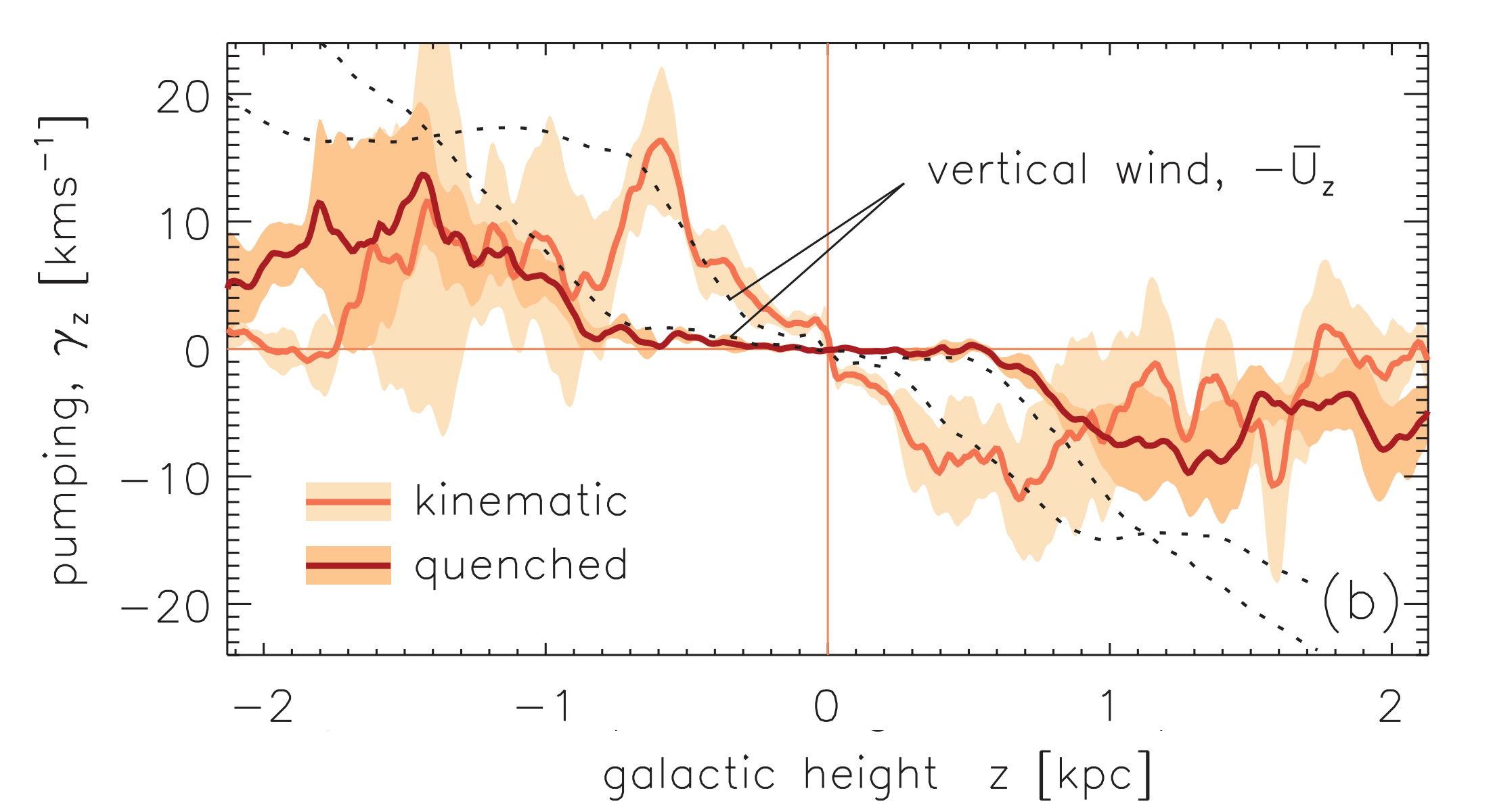
In Figure 6 we reproduce results from the work of Gressel et al. 2008b, who performed simulations of dynamos from supernova-driven turbulence in a portion of a stratified galactic disk. Using the TFM with the Nirvana code, they found that increases away from the midplane and that this leads to turbulent pumping toward the midplane, which is given by . The pumping velocity corresponds to off-diagonal components of the tensor, which they confirmed. In particular, the pumping velocity in the direction is given by , where the subscript denotes cylindrical radius. The pumping, also termed turbulent diamagnetism (SS22), pushes the magnetic field toward the midplane and thereby strengthens the dynamo (Brandenburg et al. 1993). Surprisingly, this pumping increases toward smaller scales (Gressel & Elstner 2020).
9.5 Nonlocality in space and time
It was soon realized that the results for and always depend on the wavenumber . This is explained in the box “Evolution equation for nonlocality in space and time”. For many turbulent flows, the components of both and decline with increasing values of in a Laplacian fashion approximately proportional to , where depends on details of the flow. In this relation, the value of the empirical coefficient varied between 0.1 and 0.5, depending on the nature of the turbulent flow (Rheinhardt & Brandenburg 2012).
The significance of nonlocality is that the transport coefficients become effectively quenched when the mean field is of small scale, i.e., smaller than the integral scale of the turbulence. Especially near boundaries, where sharp boundary layers may occur in calculations that ignore nonlocality, the actual field would be smoother. In fact, sharp contrasting structures have been found in earlier galactic dynamo simulations (Moss 1996). Such results would need to be revisited in view of the importance of nonlocality effects.
[t]
10 Evolution equation for nonlocality in space and time
In Fourier space, the simplest empirical approximations to the spatial and temporal nonlocalities, as obtained with the test-field method, can be combined to a single expression, which reads
| (SB8) |
where and . Moving the denominator to the left-hand side, the equation becomes
| (SB9) |
which, back in real space, becomes a simple evolution equation with a diffusion term on the right-hand side:
| (SB10) |
This equation for the electromotive force is still only an approximation, because there are in general also larger powers of and , but it provides a substantial improvement over the local formulations.
Even more important than spatial nonlocality is temporal nonlocality. It is also termed a memory effect, because it implies that the electromotive force depends not just on the magnetic field at the current time, but also on the field at earlier times. To leading order, the Fourier-transformed kernel of temporal nonlocality is proportional to , where is the turbulent turnover time. Thus, the electromotive force diminishes with increasing frequency , but there is also a new imaginary component that was absent otherwise. This can lead to new dynamo effects such as that responsible in the dynamos for the Roberts flows II and III; see the box box on “Dynamos from the memory effect”. Whether those effects play a role in turbulent dynamos is unclear.
Although the memory effect may not be strong enough to produce new dynamo effects in turbulent flows, it is strong enough to produce significant phase shifts between the generation of magnetic fields in galactic arm and interarm regions. This has been studied in detail by Shukurov 1998 and Chamandy et al. 2013. Including a memory effect in numerical simulations is, in general, very cumbersome, because it requires storing the full spatial form of the mean field for many earlier times in order to evaluate the convolution integral in Equation 9. In the present case, however, and to leading order, the convolution integral can be converted into an evolution equation for the electromotive force, which is computationally much easier to solve; see Equation SB10. This approach was first proposed by Rheinhardt & Brandenburg 2012 and was applied to dynamos in spheres (Brandenburg & Chatterjee 2018). This formalism also reproduces the dynamo effect from a time delay for Roberts flows II and III; see Section 5.1, as was demonstrated by Rheinhardt et al. 2014. This is explained in the box “Dynamos from the memory effect”.
[t]
11 Dynamos from the memory effect
We emphasize, again, that dynamos from the memory effect are so far only known to occur for the Roberts flow, so the effect may be special. At this point, however, we can not exclude that the memory plays a role in galaxies, for example in connection with the strong vertical stratification leading to a pumping effect toward the midplane. With the tools now at hand, it is now easy to explain this effect.
The dispersion relation for a problem with turbulent pumping and turbulent magnetic diffusion is given by . Since , the solution can only decay, but it is oscillating with the frequency . In the presence of a memory effect, is replaced by , where is the memory time. Then, , and can be positive. This is the case for the Roberts flow discussed in Section 5.1.
12 SETTING THE SCENE FOR DYNAMO ACTION IN REAL GALAXIES
12.1 Possibilities for seed magnetic fields
The conditions in the early Universe provide several possibilities for seeding galactic dynamos. The seeds could be primordial, which generally means that they were generated during inflation or phase transitions, or they could originate from a cosmic battery. Other theories also involve later seeding from astrophysical processes. We examine these possibilities in the following sections. {marginnote}[] \entryCosmic batteryA mechanism that can generate magnetic field even when there is none initially
12.1.1 The need for sufficiently strong seed magnetic fields
In Section 3.1 we calculated an average of 70 revolutions in the Galaxy’s lifetime. This is not very much, so we have to be concerned about possible effects on the strength and shape of the initial magnetic field. Typical estimates for the growth rate of the Galactic dynamo are of the order of (Beck et al. 1996). This means that the mean magnetic field could be amplified by up to 12 orders of magnitude in about . To reach the current level of the mean magnetic field of about , we would need a seed magnetic field of about . This is just about the level that can be expected from the Biermann battery mechanism (Rees 1987). The text box “Battery mechanisms” provides some more information about the Biermann battery and other mechanisms that can generate magnetic fields in an unmagnetized plasma.
Even though the growth rate of a galactic large-scale dynamo may just be large enough for explaining the current level of the mean field of at the present time, it would be insufficient for explaining large-scale magnetic fields in very young (redshift ) galaxies. Observationally, however, such fields are believed to exist. Kronberg et al. 1992 found evidence for strong magnetic fields in a galaxy. In a more systematic search, Bernet et al. 2008 found strong RMs in quasar sightlines passing from galaxy halos. More recently, Mao et al. 2017 estimated a G, kpc-coherent magnetic field in a lensing galaxy at . The fact that the RMs of the lensed images are similar provides evidence for large-scale magnetic coherence.
To explain smaller-scale magnetic fields at equipartition levels of would still require dynamo action, but that may just be a small-scale dynamo. Since the typical dynamo growth rates scale with the turbulence turnover time, which is shorter at small scales, a small-scale dynamo is a viable seed-field mechanism, as we discuss next.
[t]
13 Battery mechanisms
The Biermann battery.
When the density and the temperature gradient in a plasma are misaligned, the electrons move down the pressure gradient, generating an electromotive force that gives rise to a magnetic field. The resulting time derivative of the magnetic vector potential is then
| (SB11) |
where and are the electron number density and pressure, the speed of light, and the electron charge.
The Durrive battery.
Massive stars are surrounded by a region of ionized gas. Durrive & Langer 2015 proposed that an electromotive force should be created by the surplus momentum transferred to the electron after the ionization of an atom. Then, the uncurled induction equation for zero initial magnetic field becomes:
| (SB12) |
where is the rate of momentum transfer to the electrons and Equation SB12 also includes the Biermann battery.
In the early Universe, the Biermann battery can appear from local fluctuations in the sound speed right after recombination (Naoz & Narayan 2013) and later, around rippled shocks, while both battery mechanisms should operate around ionization fronts (Subramanian et al. 1994, Kulsrud et al. 1997, Gnedin et al. 2000). Garaldi et al. 2021 performed cosmological simulations testing, among other scenarios, the efficiency of the Biermann and Durrive battery terms through cosmic time. They found that, although the two batteries behave similarly, the Durrive term produces systematically weaker magnetic fields by approximately three orders of magnitude.
13.0.1 Small-scale dynamos as a seed for the large-scale dynamo
All dynamos require seed magnetic fields—even small-scale ones. However, a small-scale dynamo grows much faster than a large-scale one. It would therefore be able to produce equipartition strength magnetic fields from much weaker seeds. The idea has been discussed by Beck et al. 1994.
Another related idea is to produce galactic seed magnetic fields in the first stars. The simplest form of this idea is that stars could pick up a Biermann seed, which would then be amplified though a stellar dynamo and get ejected with a supernova explosion at the end of the star’s life. This scenario has been explored in many cosmological simulations (Beck et al. 2013, Katz et al. 2019, Vazza et al. 2017, Martin-Alvarez et al. 2021), and shows that it can, in fact, magnetize galaxies very efficiently. However, these simulations use unrealistically high values for the supernova-injected magnetic field (Ntormousi et al. 2022). Those fields could then well be large-scale ones, i.e., on the scale of stars, but those would grow on an even shorter timescale, because stars are much smaller than the envisaged turbulent eddies in the interstellar medium. Young stars and also their surrounding accretion disks can host powerful dynamos that also drive magnetized winds; see the estimates in Brandenburg 2000 and corresponding mean-field simulations by von Rekowski et al. 2003. Those winds could magnetize the surrounding interstellar medium and could well produce much more efficient seeds for the galactic dynamo than any battery mechanism. The wind-based injection model would be a viable alternative to the uncertain supernova seeding often used in cosmological simulations.
13.0.2 Battery versus plasma instabilities
When the electron distribution is anisotropic and the magnetic field is not too weak, the Weibel instability (Weibel 1959) can amplify the magnetic field, Typically, the Weibel instability generates very small-scale fields. Nevertheless, it could play a role in an intermediate regime when the Biermann battery has generated a sufficiently strong magnetic field. This is also in an agreement with recent laser plasma experiments that have accessed a regime relevant to astrophysical dynamos (Schoeffler et al. 2016).
[] \entryWeibel instabilityOccurs in a nearly homogeneous plasma when there is an anisotropy in velocity space
13.0.3 Primordial seed magnetic fields
In the early Universe, inflation and phase transitions, such as the decoupling of the weak force and the electromagnetic force or the formation of hadrons from quarks, may have produced hydromagnetic turbulence (Widrow 2002). Owing to the lack of further energy input, any magnetic field generated at that time would be slowly decaying. The dilution of the magnetic field due to the expansion of the Universe is always scaled out by talking about the comoving magnetic field, which is , where is the scale factor of the Universe. When time is being replaced by conformal time, , the MHD equations, during the radiative era, have their usual form without expansion factors (Brandenburg et al. 1996). Hereafter, the tildes are therefore dropped.
Not much is known about the strength of the comoving magnetic field today. There are only constraints. Upper limits can be derived from Big Bang nucleosynthesis (BBN) constraints; see Grasso & Rubinstein 1995 and Kahniashvili et al. 2022 for recent work taking into account the decay of the magnetic field between the moment of generation and the time of BBN. A lower limit on the present-day magnetic field strength has been proposed on the grounds that magnetic fields would prevent the reconnection of pair-created electrons and positrons when the TeV photons from powerful blazars interact with the extragalactic background light (Neronov & Vovk 2010, e.g.,). Note, however, that the validity of this technique may have a systematic uncertainty in that plasma instabilities could potentially also provide an explanation for the non-observation of GeV halos (Broderick et al. 2012).
Simulations by Sironi & Giannios 2014, confirm that plasma instabilities do indeed operate, but they only account for about 90% of the loss of GeV photons and the suppression of the remaining 10% would still need to be explained by the presence of magnetic fields. Similar conclusions were reached by Alves Batista et al. 2019, who performed detailed simulations for individual blazars.
The lower limits derived by Neronov & Vovk 2010, which become less stringent for larger length scales, provide an exciting motivation for primordial magnetogenesis scenarios. At the present time, those primordial magnetic fields may have strengths in the range of to (see Subramanian 2016, for a review), and could act as seed magnetic fields for any subsequent dynamo processes – once sufficient kinetic energy becomes available. These seeds, if confirmed, would not only be stronger than those from batteries, but they would also be present in the voids. Figure 7 shows the expected magnetic field ranges as a function of the typical scale of the magnetic field. For a nonhelical magnetic field, there are still magnetic helicity fluctuations. They constrain the decay such that the correlation integral of the local magnetic helicity is conserved (Hosking & Schekochihin 2021). This leads to a decay with and , so that (Hosking & Schekochihin 2022).
The first stars are expected to form about after the Big Bang, marking the beginning of the reionization epoch. After that, galaxies start growing through continuous gas accretion and mergers (Dayal & Ferrara 2018). Since dynamo action is fastest at small length scales, the magnetic field generation during the formation of the first collapsing structures is potentially important and may have produced a stronger seed magnetic field for the subsequent global galactic dynamo. Strong magnetic fields may also affect galaxy and large-scale structure formation of the Universe (Kahniashvili et al. 2013).

13.0.4 Primordial fields during structure formation
Modern numerical simulations of cosmological large-structure formation are taking into account the evolution of the magnetic field, seeded by the various mechanisms outlined above. A central question in these studies is whether the topology and strength of these primordial fields leave measurable signatures on the cluster or galaxy structures.
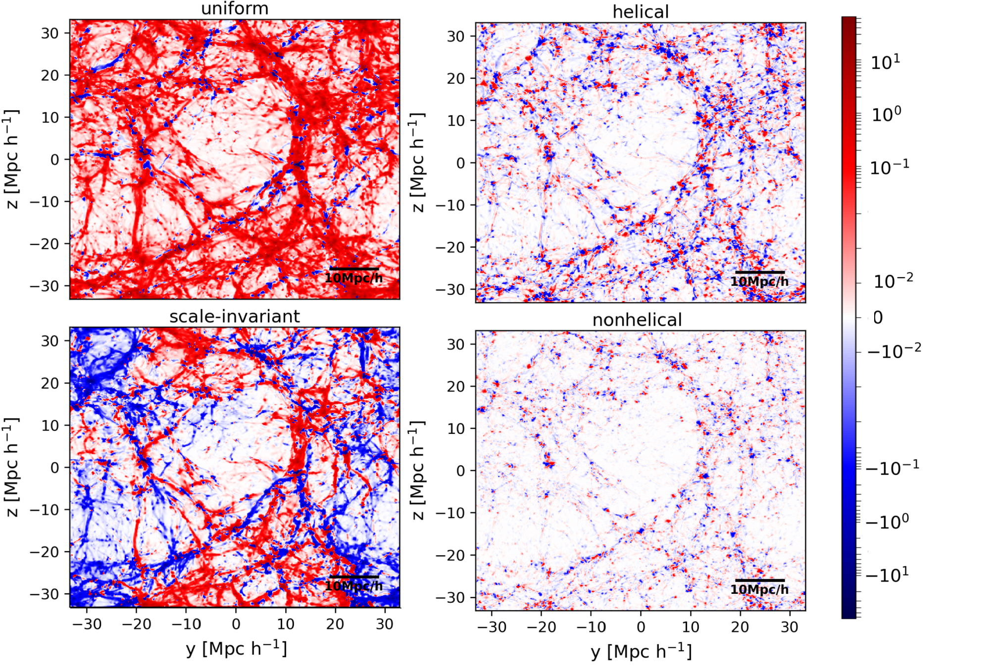
Vazza et al. 2017 performed a comprehensive suite of cosmological simulations using different magnetogenesis mechanisms: a uniform seed, meant to simulate the magnetic field created by inflation, a seed that follows the distribution of density perturbations to approximate the magnetic field generation by a Biermann battery, a seed that approximates the turbulent dynamo amplification, and an astrophysical seed that simulates the injection of magnetic fields by stellar sources. They find that, at , all mechanisms agree on the cluster magnetization (which they were designed to reproduce). However, there are large differences in the magnetic field structure both on galaxy scales and in the voids. Recently, Mtchedlidze et al. 2022 explored a more diverse set of primordial magnetic fields, including uniform and scale-invariant inflationary fields, as well as helical and non-helical fields from the radiation-dominated epoch. They also reported that the final magnetic field distribution retained a memory of the initial seed. This can be seen from Figure 8, where we show maps of Faraday rotation at the present time. The simulations started at a redshift of with the four initial conditions discussed above.
The above works use a uniform spatial resolution, which offers the advantage of an unbiased view of cosmological magnetic field evolution. However, models with adaptive resolution can give a more detailed view of the magnetic field on galaxy scales, while following their cosmological history. One recent example is the work of Garaldi et al. 2021, who explored the evolution of cosmological volumes and zoom-ins using four different mechanisms for magnetic field generation: primordial, Biermann battery, Durrive battery, and stellar seeds. They report, contrary to the findings of the uniform-resolution, large-volume works mentioned above, that the initial conditions are forgotten by redshift . However, none of their initial conditions contained magnetic helicity, which should not have decayed.
Marinacci & Vogelsberger 2016 and Martin-Alvarez et al. 2020 focused on the effects of cosmological magnetic fields on galaxy formation. They found that fewer, smaller galaxies form for stronger primordial fields. As mentioned in Section 3.1, Martin-Alvarez et al. 2021, traced the evolution of the primordial field and the field injected by stellar sources separately (see Figure 3). They achieved this by adding two tracer induction equations to the code, one for each seed. These induction equations are not connected to the gas evolution, but only follow the evolution of the two fields as it would be if they were independent of each other. They found that their evolved galaxies contain a mixture of both: metal-poor gas at the galaxy’s outskirts containing mostly primordial fields with large-scale coherence and supernova (SN)-enriched gas containing mostly fields of stellar origin with small-scales coherence. The cold, star-forming gas contains a mixture of the two. However, in agreement with the Garaldi et al. 2021 result, the origin of the galactic magnetic field becomes practically indistinguishable very early on without the tracers. All these simulations result in microgauss magnetic fields, but their length scales are typically too small to explain the fields seen in actual galaxies.
The results of these comprehensive simulations point to a complex picture in which various seeding mechanisms combine to give the initial and boundary conditions for dynamos on different scales and different epochs. They also point to cluster scales – rather than galaxy scales for an answer regarding the origin of cosmic magnetic fields.
13.0.5 Possible importance of cluster mergers
Mergers of galaxy clusters could amplify large-scale magnetic fields quickly to near-equipartition strengths. The merger itself could stretch a pre-existing field and amplify it in conjunction with the existing (possibly helical) background turbulence. One could then think of this as some kind of dynamo, where the effect is associated with the large-scale shear generated during the merger. Such simulations were produced by Roettiger et al. 1999.
The study of the relevance of cluster mergers to dynamos has not been followed up in recent years. In the meantime, there have been many relevant advances in dynamo theory in connection with time dependence of the flow and in the context of measuring field transport coefficients. In view of these advances, this approach might deserve more detailed follow-up studies in the future. However, there are similarities with recent studies of gravitational collapse dynamos that will be discussed next.
13.1 Dynamos from gravitational collapse and other instabilities
By the time the first gravitationally bound structures (stars or galaxies) formed, any primordial turbulent velocities from the processes we mention in Section 13.0.3 had already decayed. However, the assembly into these first structures certainly generated large amounts of turbulent kinetic energy, which could have triggered dynamo action.
Several numerical works show that the formation of the first stars is ideal for amplifying nG (Sur et al. 2010, Sur et al. 2012, Federrath et al. 2011), or even just (Schober et al. 2012) fields to equipartition values through a small-scale dynamo. Gravitational compression can amplify the field further, although in the presence of turbulence, the resulting dependence of the magnetic field on the density is weaker than the prediction from ideal flux freezing (Sur et al. 2012). While flux freezing predicts , the theory of Xu & Lazarian 2020, which includes the turbulent dynamo, predicts that , where the scaling of the small-scale dynamo enters as an assumption. This remarkable agreement with the simulation results of Sur et al. 2012 is taken to be suggestive of the importance of reconnection diffusion and the breakdown of flux-freezing (Xu & Lazarian 2020), which makes compressional amplification less efficient.
However, the results obtained so far still leave some questions unanswered. For example, is it possible to explain the slow-down of compressional field amplification even in the absence of dynamo action? Although this may be an academic question, it could be answered by performing collapse simulations in two dimensions, when dynamo action is impossible. Also, it would be interesting to see the early magnetic field growth starting from a much smaller initial magnetic field. In fact, the theory of Xu & Lazarian 2020 does not really address when the dynamo is excited, but focusses on the discussion of the nonlinear regime of a supercritical dynamo.
13.1.1 Nature of collapse dynamos
An important tool for characterizing dynamo action in time-dependent flows such as decaying turbulence or gravitational collapse, is to compare the work done against the Lorentz force with the Joule dissipation rate, and to look at different contributions to the Lorentz work term. These work and dissipation terms emerge when deriving the evolution equation for the magnetic energy density. Taking the dot product of Equation 2 with , averaging, and ignoring surface terms, we obtain
| (10) |
Using , one can write the first term on the right-hand side of Equation 10 as the work against the Lorentz force. Two further refinements can then be employed (Brandenburg & Ntormousi 2022). First, one can decompose to write , where and . The second term, , vanishes for 2-D magnetic fields oriented in the plane and describes therefore the work term associated with 2-D compression, stretching, and bending, such as in Equation 1. Second, one can decompose into contributions from the magnetic pressure force, the tension force, and curvature force. The corresponding work terms are then referred to as (for compression), (for tension force, i.e., along the field), and (for the curvature force, i.e., perpendicular to the field).
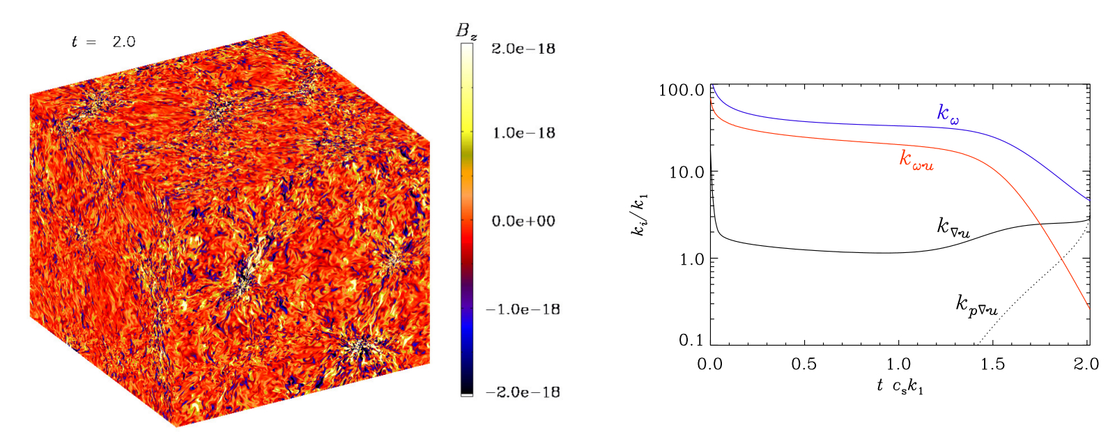
To determine the reality and nature of dynamo action during a turbulent self-gravitational collapse more carefully, Brandenburg & Ntormousi 2022 computed the aforementioned terms that enter the magnetic energy balance. The basic conclusion is that there is indeed dynamo action during the early phase of the collapse while the initial turbulence is slowly decaying, but that dynamo action diminishes when the flow becomes dominated by 3-D compression toward the various collapsing potential minima, where only the irrotational flow component gains in strength, which, however, does not (or not much) contribute to dynamo action in their simulations. In Figure 9 we visualize the collapsing magnetic field from Brandenburg & Ntormousi 2022, the diminishing of the vorticity, expressed here as a wavenumber , the gain of compressive motions, here expressed through , along with several other quantities, and , characterizing the work done by compression and the amount of kinetic helicity, respectively. A potential problem with the simulations of Brandenburg & Ntormousi 2022 is the relatively short collapse time compared with the turnover time of the turbulence.
13.1.2 Magneto-buoyancy and magneto-rotational instabilities
These instabilities can drive turbulence and may play important roles in parts of the galaxy. {marginnote} \entryMagneto-rotational instabilityarises in a magnetized, rotating disk when the angular velocity decreases with distance. Buoyancy may be driven by cosmic rays inflating flux tubes and are thought to speed up the dynamo (Parker 1992, Hanasz et al. 2013). The magneto-rotational instability (Balbus & Hawley 1991) can drive turbulence from the kinetic energy in the shear. It can also play a role in the outer parts of the galaxy were supernova driving is less efficient (Piontek & Ostriker 2007).
14 GALACTIC MEAN-FIELD DYNAMOS
14.1 Global magnetic field structure
One of the strongest existing tests for dynamo theories is the predicted structure of the large-scale magnetic field contrasted to observations. In the next sections we outline the predictions from different models.
14.1.1 Early analytic approaches
The idea that the large-scale magnetic field of galaxies could be explained through an dynamo was formulated early on (Vainshtein & Ruzmaikin 1971, Parker 1971), just after the first successful mean-field models were proposed for the Sun and Earth. An important early result was the finding that the most preferred magnetic field mode in flat geometries like galaxies is quadrupolar, i.e., the toroidal field is even about the midplane. [Here and elsewhere, quadrupolar means not just a quadrupole, but all modes of even symmetry about the midplane (Krause & Rädler 1980).]
In view of many early claimed discoveries of BSS fields (Sofue et al. 1986, for a review, see), an important question in those early days concerned the possibility of preferred nonaxisymmetric magnetic fields. Such modes were never found. However, when the assumption of what is known as the pure approximation was made, i.e., the toroidal field is only generated by differential rotation ( effect) and the effect is {marginnote}[] \entryASS and BSS fieldsdefined as and magnetic fields and vary with azimuth like . neglected in the generation of the toroidal magnetic field, nonaxisymmetric modes where found to be excited, although the growth rates of the corresponding ASS fields were always larger; see Section 3.1. This approximation turned out to be not permissible, when the magnetic field is nonaxisymmetric.
14.1.2 Boundary conditions
Standard dynamo problems are usually formulated with vacuum boundary conditions, i.e., the magnetic field is current-free and extends to infinity outside the domain (Krause & Rädler 1980). However, such boundary conditions can only be formulated for spheres or ellipsoids, but not for cylinders, for example. Stix 1975 employed ellipsoidal coordinates and obtained an axisymmetric solution. Contrary to Parker 1971, he found that oscillatory solutions occur only at substantially larger dynamo numbers. {marginnote} \entryDynamo numberDefined as , where and are mean-field magnetic Reynolds numbers associated with differential rotation and -effect, respectively. Unfortunately, the implementation of ellipsoidal coordinates in a numerical code is rather cumbersome. This led to the approach of embedding the galaxy in a sufficiently large poorly conducting halo, which itself is then contained either in a cylinder with perfectly conducting boundaries (Elstner et al. 1990), or in a sphere with vacuum boundaries (Brandenburg et al. 1990). These two alternatives are rather different from each other, but the hope is that these boundaries are far enough away from the physical boundaries that these differences are without consequence.
14.2 Dynamo models for specific galaxies
Various attempts have been made to produce dynamo models of individual galaxies. One such example is M31, i.e., the Andromeda galaxy. Its magnetic field is often described as a ring field. It is also often regarded as an analog of the Milky Way. Corresponding models have been presented by Poezd et al. 1993 using nonlinear quenching. An important challenge here is to reproduce the right pitch angle of the magnetic field and its radial dependence; see Shukurov 2000 and Fletcher et al. 2004 for detailed discussions.
Another interesting case is M81, whose magnetic field is possibly predominantly nonaxisymmetric. This was difficult to explain. Moss et al. 1993 showed however that such a field could result from an initial magnetic field that might have survived for long enough times, at least in the outer parts of the galaxy. Yet another very different case is NGC 6946, whose field may consist of structures usually termed magnetic arms. Magnetic arms are often interlaced with the stellar arms, but can also be phase-shifted relative to them; see Shukurov 1998 and Chamandy et al. 2015 for a more detailed discussion, and Beck et al. 2019 for recent updates.
Finally, we mention the magnetic fields in the halos of the edge-on galaxies NGC 891 and NGC 4631. Brandenburg et al. 1993 and Elstner et al. 1995 found that the observed polarization vectors could only be reproduced when there is a strong enough outflow. We return to this in Section 14.5.
14.3 Galactic models with magnetic helicity flux
In Section 8.1 we have discussed the potential importance of magnetic helicity fluxes. It is often believed that they would be required to explain strong magnetic fields in galaxies. Here, we demonstrate the effect of magnetic helicity fluxes in specific models. Shukurov et al. 2006 have presented nonlinear models in a one-dimensional geometry using the magnetic helicity flux associated with a galactic fountain flow. The main nonlinearity was here given through the dynamical quenching formalism with advective magnetic helicity fluxes included, similarly to what was discussed in Section 8.1. The authors found that a magnetic helicity flux does indeed lead to larger magnetic field amplitudes provided the magnetic helicity flux is strong enough. In their model, the helicity flux was accomplished through a galactic fountain flow with a speed of at least . More detailed studies have been performed by Prasad & Mangalam 2016, who also included advective and diffusive magnetic helicity fluxes.
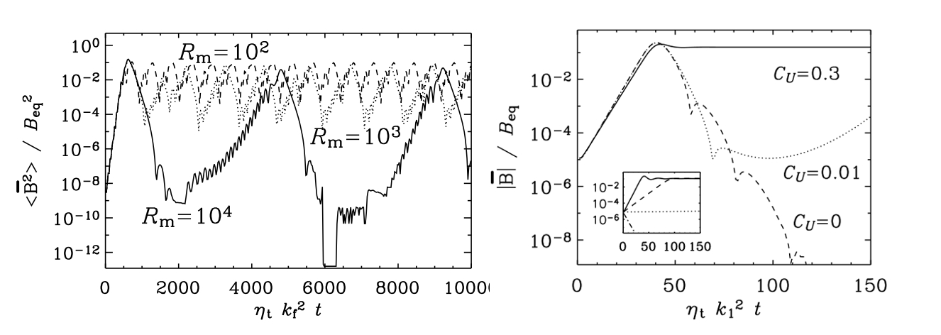
There is some uncertainty regarding the main contributors to the magnetic helicity flux; see the more recent study by Vishniac & Shapovalov 2014. In addition to advection, shear could modify the turbulent correlations in such a way as to transport magnetic helicity efficiently outward. First proposed by Vishniac & Cho 2001, this can lead to episodic magnetic field amplification, especially as is increased; see Brandenburg & Subramanian 2005b and the left-hand side of Figure 10. On the right-hand side of Figure 10, we reproduce the simulation result of Shukurov et al. 2006 with an advective magnetic helicity flux. In the models with insufficient advective flux, the magnetic energy decreases to very small values. The earlier simulations by Brandenburg & Subramanian 2005b, their Figure 7, with somewhat smaller values of the magnetic Reynolds number showed that the magnetic field can recover after some time, but then, again, it begins to fall off, just like what is seen in Figure 10. However, one may want to remain sceptical about whether these fluxes really do alleviate the catastrophic quenching, because so far this has been seen only in mean-field models and not yet in actual turbulence simulations.
14.4 Galactic rotation measure signature
In Section 3.1 we mentioned the historical importance of RM studies for distinguishing between an ASS field, characteristic of dynamo models, and a BSS field, characteristic of a wound-up primordial fields. The subsequent findings of RM studies indicate that galactic magnetic field evolution might be more complex than this simple dichotomy.
At the time of the review of Sofue et al. 1986, most galaxies were thought to be of BSS type; the authors listed seven out of 11 galaxies as having a BSS field. However, more accurate subsequent surveys confirmed a predominantly BSS type structure for only M81 (Krause et al. 1989). In a later review, Beck et al. 1996 listed the field structures for 33 galaxies. The picture became more complicated, with four examples primarily of ASS fields (albeit two where marked as uncertain). The dominance of ASS over BSS continues to persist even today. For M33, Tabatabaei et al. 2008 found an axisymmetric field in the inner regions and a superposition of axisymmetric and bisymmetric fields in the outer regions. Beck 2015b observed a weak () axisymmetric field in IC 342, and Beck et al. 2020 found a dominating ASS field in M31 combined with a six-times weaker BSS component.

Classifying the Milky Way’s magnetic field structure is much harder. The existing parametric models of the Galactic magnetic field are largely based on full-sky RM maps of extragalactic sources (Oppermann et al. 2015, Hutschenreuter et al. 2022, e.g.,) and synchrotron emission maps of the Milky Way (mainly from the Wilkinson Microwave Anisotropy Probe; see Page et al. 2007, Bennett et al. 2013, see also Figure 11). The model of Sun et al. 2008 assumes an axisymmetric spiral with a reversal in the inner 5 kpc. Jansson & Farrar 2012 include magnetic spiral arms and an X-shaped field in the halo (see also Section 14.5 for the observational motivation). Jaffe et al. 2010 also fit magnetic spiral arms to the disk data, also including the random magnetic field component. Terral & Ferrière 2017, using analytic forms for the 3-D field, conclude that a bisymmetric () halo field best fits the RM data. However, West et al. 2020 found evidence for an axisymmetric () quadrupolar magnetic field with a small net vertical component in RM. A newer analysis (Dickey et al. 2022) shows that a combination of an axisymmetric and a bisymmetric mode, based on analytical galactic dynamo models from Henriksen et al. 2018, best explains the large-scale morphology of the Galactic RM data. As the quality of the observational data improves, a complex picture of galactic magnetic field morphology emerges, including that of the Milky Way.
14.5 Synchrotron emission from mean-field models
Synchrotron emission provides an important means of measuring the magnetic field in galaxies and comparing models with simulations (see Beck et al. 2019, for a review on bridging dynamo models and observations).
Early attempts of computing the polarized synchrotron emission from models were presented by Donner & Brandenburg 1990, who computed the linearly polarized emission from galactic mean-field models, which contained both axisymmetric and nonaxisymmetric magnetic fields. They confirmed the idea of distinguishing these modes by measuring the RM along a ring around the galaxy. Another example was the computation of linear polarization from the magnetic field on both sides of the midplane in edge-on galaxies. In galaxies seen edge-on, synchrotron emission reveals X-shaped halo magnetic fields (Golla & Hummel 1994, Tüllmann et al. 2000, Krause et al. 2006, Stein et al. 2019, Krause et al. 2020, e.g.,). Although the 3-D morphology of these fields is unknown, the X-shaped signature can be reproduced by dynamo models that include an outflow (Brandenburg et al. 1993, Elstner et al. 1995). The resulting magnetic fields were thought to have quadrupolar symmetry also in the halo, but this now seems to be ruled out by new observations (Mora-Partiarroyo et al. 2019). An alternative would be a dynamo in the halo itself, which could produce dominant dipole modes (Brandenburg et al. 1992, Moss & Sokoloff 2008).
At long radio wavelengths, the synchrotron emission from even just a uniform magnetic field suffers depolarization from the superposition of Faraday-rotated contributions. However, if the magnetic field is helical, the polarized intensity can either enhance the depolarization if helicity and RM have opposite signs, or it can cancel it if they have the same sign (Brandenburg & Stepanov 2014, Horellou & Fletcher 2014). This leads to a correlation between polarized intensity and RM (Volegova & Stepanov 2010), which has now been used by West et al. 2020 to characterize the Galactic magnetic helicity. Future observations with the Square Kilometre Array are expected to reveal much more detailed information on magnetic helicity using a continuous band of wavelengths (Beck et al. 2015).
The synchrotron intensity gives an indication about the magnetic field strength. It is proportional to the product of the density of relativistic cosmic ray electrons and a power close to 2 of the local magnetic field component perpendicular to the line of sight. However, the relativistic cosmic ray electron density may itself depend on the local magnetic energy density, because cosmic rays and magnetic fields have supernova explosions as a common source of energy. These arguments have been reviewed by Seta & Beck 2019, who also make comparisons with numerical simulations of cosmic ray confinement by a local dynamo-generated magnetic field, similar to what was done earlier by Snodin et al. 2006. Seta & Beck 2019 conclude that the commonly made assumption of an equipartition between cosmic ray and magnetic energy densities is not valid on scales smaller than at least . They argue that ignoring the nonlinear dependence of the synchrotron emission on the plane-of-the sky magnetic field component can lead to an overestimation of the actual magnetic field by up to a factor of 1.5.
An interesting comparison between radio synchrotron and dust polarization in emission can be found in Borlaff et al. 2021 for M51. They find that the magnetic pitch angles of the two tracers differ, with the dust polarization showing a more tightly wound spiral than the radio. In light of this and forthcoming comparisons, predictions from dynamo models should take into account the multi-phase nature of the ISM.
14.6 and polarizations
The linear polarization described by Stokes and can also be expressed in terms of the rotationally invariant parity-even polarization and the parity-odd polarization, as is commonly done in cosmology (Seljak & Zaldarriaga 1997, Kamionkowski et al. 1997). Here, the symbols and have nothing to do with electric and magnetic fields, except that both can qualitatively be described as gradient-like and curl-like fields. It is important to stress, however, that and are only defined on a 2-D surface. Therefore, the parity-odd polarization has no immediate correspondence with the helicity of the underlying magnetic field.
Mathematically, and are obtained as the real and imaginary parts of a quantity with
| (11) |
and are coefficients that have been computed as
| (12) |
with being the spin-2 spherical harmonics and the asterisk denoting the complex conjugate.

Brandenburg & Brüggen 2020 found that the polarization averaged over Galactic longitude is very small owing to longitudinal cancelation, but there is a small net hemispheric antisymmetry. This is shown in Figure 12, where we plot the Galactic mode polarization together with the longitudinally averaged mode polarization. It may be tempting to associate this hemispheric dependence with that anticipated for the effect, which is also a parity-odd quality with hemispheric sign change. However, the observed hemispheric antisymmetry is actually explained by the spiral nature of the magnetic field. Looking toward northern and southern galactic latitudes yields mirror images of each other, which explains the observed hemispheric antisymmetry of the mean .
15 TURBULENCE SIMULATIONS OF GALACTIC DYNAMOS
15.1 Physical parameters of the ISM
The interstellar gas can be found in various phases, characterized by different temperatures, densities, and degrees of ionization. The neutral, atomic gas is found in a cold () and a warm () phase, usually termed the cold and warm neutral media (CNM and WNM, respectively). The ionized gas is also found in a hot () and a warm () phase (HIM and WIM, respectively). Finally, the densest and coldest () gas is mostly molecular medium (MM), with a very low ionization fraction.
Dynamos can easily be excited in the interstellar medium, since all phases (apart from the MM) are characterized by large values of Re, , and , although these vary greatly between phases; see Table 3, with order-of-magnitude values taken from Ferrière 2020 and Draine 2011. This vast range of parameters also poses a challenge for accurately modeling interstellar turbulence. At large , the small-scale magnetic energy tends to dominate and the dynamo returns much of the magnetic energy back into kinetic energy (Brandenburg & Rempel 2019). However, no effect on the large-scale dynamo has been reported as yet.
| Phase | HIM | WIM | WIM | CNM | WNM | MM |
| Re | ||||||
Most of the numerical work on ISM turbulent dynamos so far has been isothermal (Schekochihin et al. 2004, Seta et al. 2020, e.g.,). In an interesting extension, Seta & Federrath 2022 modelled a small-scale dynamo in driven turbulence simulations of a two-phase ISM and identified the processes responsible for vorticity generation in each phase. They found that the magnetic to turbulent kinetic energy ratio is lower in the cold phase. This will be discussed in more detail in Section 15.3.
15.2 Numerical approaches
Including magnetic fields in simulations of astrophysical systems is a non-trivial task because the chosen discretization must obey the zero divergence constraint. In Eulerian codes, a commonly used approach is the Constrained Transport (CT) scheme (Evans & Hawley 1988), which ensures by defining the magnetic field components on cell faces. However, no similar scheme is applicable to Lagrangian codes such as Smoothed Particle Hydrodynamics (SPH), which rely on divergence-cleaning algorithms (Brackbill & Barnes 1980, Powell et al. 1999, Dedner et al. 2002, e.g.,).
| Code name | Approach | Other properties | |
| AREPO1 | -clean |
| |
| ENZO2 | CT or -clean |
| |
| FLASH3 | CT or -clean |
| |
| Gadget4 | -clean | SPH | |
| Nirvana5 | CT | AMR, Godunov (Riemann) | |
| Pencil Code6 | centered finite diff., sixth order | ||
| RAMSES 7 | CT | AMR, Godunov (Riemann) |
- 1
- 2
- 3
- 4
- 5
- 6
- 7
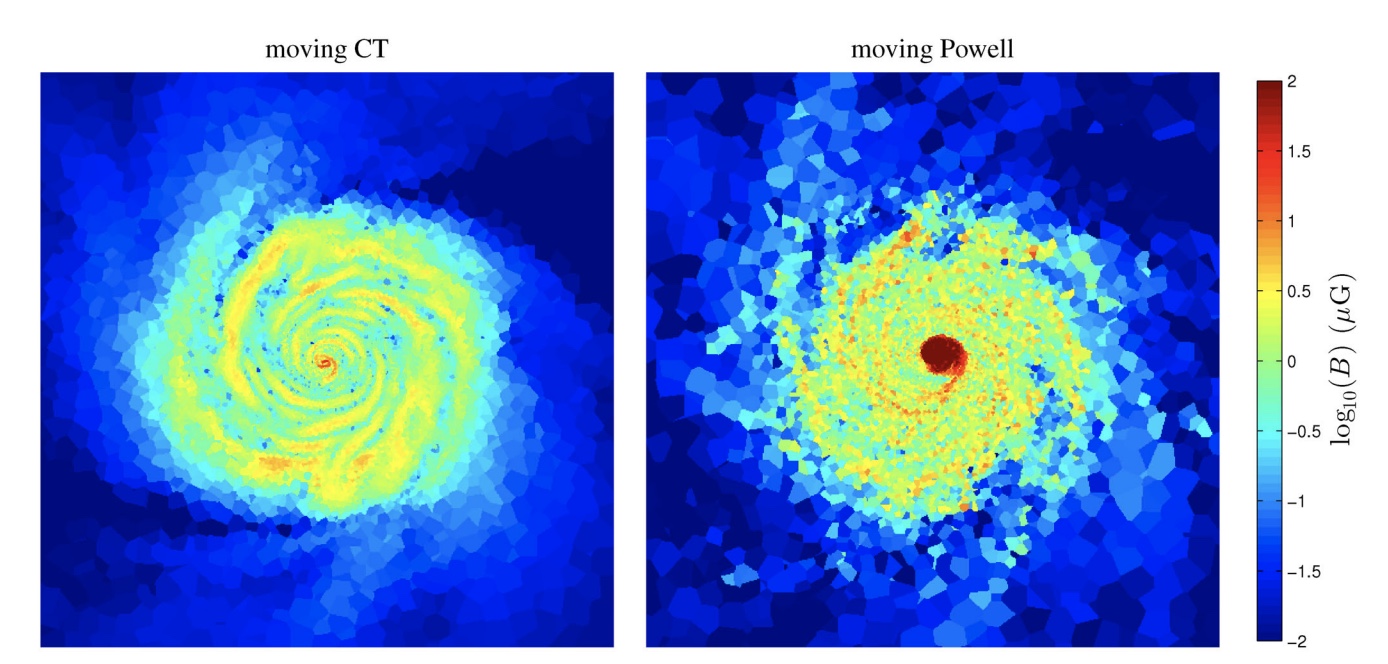
Lagrangian codes are particularly well-suited for modeling galaxies and cosmological volumes due to the natural adaptation of the resolution to areas of interest. They are also naturally Galilean-invariant. However, their dependence on divergence cleaning poses a significant drawback when modeling astrophysical dynamos. This was clearly demonstrated by Mocz et al. 2016, who compared CT and divergence cleaning approaches, both implemented on the moving-mesh code AREPO. They found that divergence cleaning systematically creates artifacts that mimic physical effects. Some of these artifacts are illustrated in Figure 13.
Out of these effects, particularly notorious for dynamo studies is an artificial increase of the magnetic energy when using scalar divergence-cleaning schemes, as pointed out by Balsara & Kim 2004 for supernova-driven turbulence. Another very relevant example of an artifact caused by divergence cleaning is the spontaneous production of magnetic helicity, which has been found by Brandenburg & Scannapieco 2020, who compared simulations that employed a divergence cleaning algorithm with one that advances instead the magnetic vector potential, , so that is always divergence-free. They found that, for a helically driven flow in a periodic domain, spurious net magnetic helicity is generated on dynamical timescales. An interesting experiment by Tricco et al. 2016 compared an SPH code to the FLASH grid code, both using divergence cleaning, in simulations of turbulent dynamos. They found very good agreement between the codes, both in the growth rates and the saturation level of the dynamo. This suggests that potential problems with divergence cleaning may not be severe.
Yet another method of dealing with the constraint is to employ the Euler or Clebsch potentials. However, this method only works in the strictly ideal case when the microphysical magnetic diffusivity vanishes; see Section 3.2. As we have stressed in Section 3.2, the addition of an almost negligibly small diffusivity to the evolution equations for the Euler potentials does not correspond to any physical magnetic diffusivity and leads to wrong results where no dynamo is possible—even for flows that are fast dynamos (Brandenburg 2010).
Table 4 outlines some characteristics of the codes mentioned in this review. Next to each code we have mentioned the works cited in this review that use it. The fact that many of them have to rely on divergence cleaning methods is evidence of the difficulty in dealing with the divergence problem, but also a sign to use caution when interpreting the results in the context of dynamo action.
15.3 Local dynamo simulations of galaxy portions
Simulating the magnetic field evolution over an entire galactic disk is another challenging task, due to the vast range of dynamical scales of the problem and the large shearing velocities involved. One approach to this challenge that can successfully capture many aspects of the problem is simulating galaxy portions. The local approach has been rather successful in the context of accretion disks, where simulations have been performed in what is known as shearing boxes. This means that the radial boundary is “shearing-periodic”, i.e., it is periodic with respect to an azimuthal position that shifts in time following the background shear flow.
Using a shearing box, Gressel et al. 2008a performed the first simulation of a galactic dynamo, including supernova-induced turbulence. It was similar to earlier multiphase simulations of supernova-driven turbulence of Korpi et al. 1999, where the magnetic Reynolds number was still too low to permit dynamo action. Gressel et al. 2008a found that the rotation frequency of the considered galaxy portion is the dominant factor in determining the dynamo efficiency, while the supernova rate did not significantly affect the efficiency of the dynamo. This finding suggests that the simulations were able to capture large-scale dynamo action, but not small-scale dynamo action. Interestingly, they also found no evidence of catastrophic quenching in the range of values explored by varying the rotation frequency of the galaxy portion. They hypothesize that this could be due to helicity fluxes. In a subsequent paper, Gressel et al. 2013 speculated about various quenching scenarios based on the magnetic field dependence, but that was just for one value of the microphysical magnetic diffusivity.
Using the Pencil Code and a similar setup, Gent et al. 2013 showed that the mean and fluctuating fields have different growth rates, indicating a co-existence of small- and large-scale dynamos. Theoretically, however, the possibility of large-scale and small-scale dynamos having different growth rates in one and the same system is not well understood (Subramanian & Brandenburg 2014).
Recently, Gent et al. 2021 sought to derive criteria for the appearance of a small-scale dynamo in simulations of interstellar turbulence. By not employing a shearing-box setup or stratification, they focused only on the effects of the supernova-driven turbulence. They confirm that, below a critical physical resistivity (i.e., a sufficiently high ), a small-scale dynamo is easily excited by ISM turbulence, a result that appears to converge at resolutions below 1 pc.
Seta & Federrath 2022 have shown that the multiphase aspect of the ISM tends to have a detrimental effect on the small-scale dynamo. This is mostly because of the stronger Lorentz force in the cold regions. Their simulations show that with solenoidal forcing, the magnetic field is mostly decoupled from the density behavior; see Figure 14. Simple compression along magnetic field lines (), perpendicular to to magnetic field lines ( for cylindrical/filamentary geometry and for disc-like/slab geometry), and spherical compression () hardly occur. One might argue, however, that in the compressive case, the cold phase shows a higher slope than the warm phase.
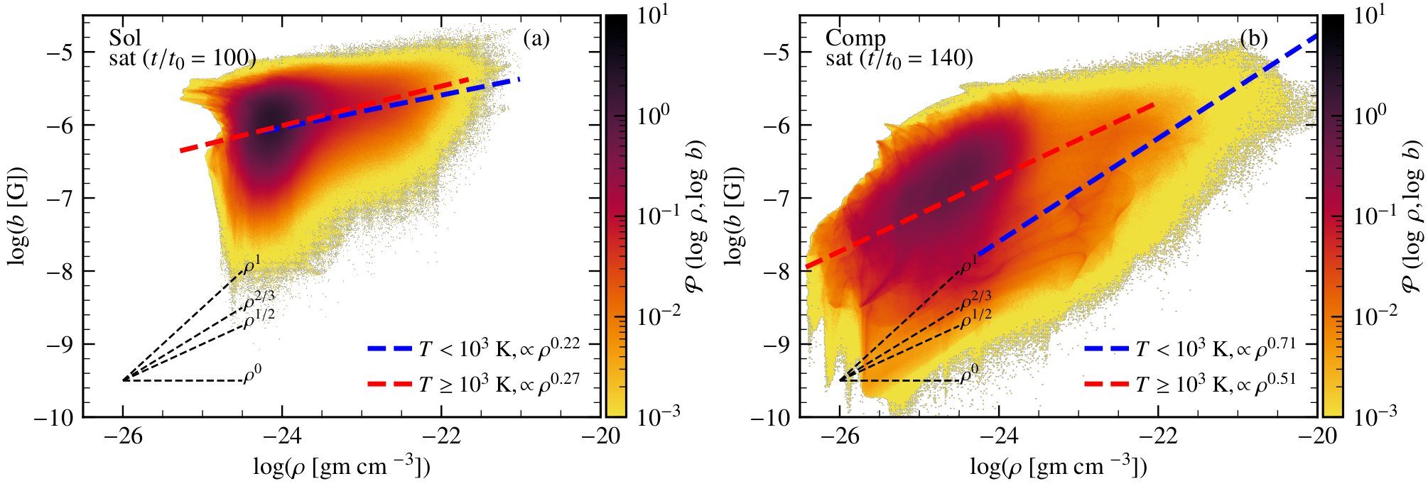
15.4 Global isolated galaxy simulations
The increasing efficiency and complexity of numerical codes and the availability of resources have led to a number of works studying the magnetic field evolution in global galaxy models. In contrast to the shearing-box approach, such models more naturally allow for the study of the large-scale dynamo. However, the limited resolution is still problematic for simultaneously capturing the small-scale dynamo, as outlined above.
Wang & Abel 2009 performed disk galaxy simulations including ordered seeds with a code similar to Enzo, using Dedner et al. 2002 divergence-cleaning. They found that the tiny seed was amplified to G levels over 500 Myr. They also noticed that the magnetic field in the cold gas saturated first. Their setup did not include stellar feedback, so the amplification process was driven by differential rotation only.
In a series of papers, Rieder & Teyssier 2016, Rieder & Teyssier 2017a, Rieder & Teyssier 2017b performed multi-component simulations of the magnetic field evolution in dwarf and Milky-Way-like galaxies using the RAMSES code and including supernova feedback. Their setup includes dark matter and stars as collisionless particles, coupled to an Adaptive Mesh Refinement (AMR) grid on which the MHD equations are solved. In the first paper of the series, the authors found signatures of {marginnote} \entry(Stellar) FeedbackThe energy and momentum deposited to the ISM by stars through radiation, winds, and supernova explosions small-scale dynamo amplification during intense feedback epochs, followed by a large-scale dynamo at later, more quiescent evolution times. In the second paper, they examined the saturation of the dynamo, which occurs at only a small fraction of the turbulent kinetic energy. They observed that, if the feedback efficiency is artificially lowered after saturation, the turbulence decays and the galaxy settles in a thin disk with an equipartition field. Rieder & Teyssier 2017b studied the magnetic field evolution in a cosmological context.
Using a similar setup and separating the mean from the fluctuating component using a median filter, Ntormousi et al. 2020 found large-scale dynamo action in a model of a massive spiral. However, their result was insensitive to the inclusion of supernova feedback. Since supernova feedback is considered an important driver of small-scale turbulence, this could mean that a small-scale dynamo was never captured in their models. This result is consistent with the Rieder & Teyssier 2016 results for the quiescent phase of galaxy evolution. However, as shown by Gent et al. 2021, the limited resolution of the simulation could be preventing the formation of a small-scale dynamo action in this quiescent phase.
Pakmor et al. 2017 performed a suite of zoom-in cosmological simulations that includes 30 galaxies using the AREPO code (called the Auriga simulations). Similarly to Rieder & Teyssier 2017b, they reported early exponential growth of the magnetic field, saturating at redshift at a few percent of the turbulent kinetic energy. Steinwandel et al. 2019 also claimed significant small-scale dynamo action in isolated galaxy models using an MHD version of the Gadget code. However, these simulations rely on the divergence-cleaning scheme that could suffer from the problems summarized in Section 15.2.
A very different approach was adopted by Rodrigues et al. 2019, who modeled galactic magnetic fields by post-processing cosmological simulation data. Specifically, they inserted galaxy parameters such as shear rate and turbulence into a parameter-fitting package that returns a suitable dynamo solution (Shukurov et al. 2019). Although this approach cannot capture the back-reaction of the magnetic field on the gas, it can give estimates on the cosmological conditions that favor mean-field dynamo action, which the authors find set in at redshift .
While each numerical approach presents certain limitations, the tentative picture painted by global numerical simulations is that the small-scale and large-scale dynamos co-exist during galaxy evolution. Taking into account the large-scale gravitational collapse of the halo, as well as internal galactic processes such as star formation, appears to be fundamental for reconstructing the observed magnetic field evolution.
Currently, the problem of catastrophic quenching we discussed in Section 7.2 remains unexplored in global galaxy models. The reason is that physical resistivity and viscosity are usually not included, so that there is no easy estimate of the range probed by each model. Exploring the effects of the inevitable numerical resistivity by performing resolution studies might also be insufficient to approach the physical solution, because the diffusion operator depends on resolution. Small-scale helicity fluxes, which could in principle appear self-consistently in these models, are not reported. It would be interesting to see in upcoming studies how helicity fluxes emerge (or not) from different subgrid models.
16 INTERACTION WITH THE CGM
It was already suggested in the previous sections that the galactic environment must play an important role in the behavior of the dynamo, because it defines the boundary conditions for its operation. The immediate environment of a galaxy is its halo, which contains large amounts of diffuse gas, and is usually referred to as the CGM.
The CGM is a powerful probe of galaxy evolution processes, because it contains traces of the cold () and hot () galactic inflows, as well as the hot (), metal-enriched outflows from feedback events (Putman et al. 2012). The CGM also contains colder gas () that can co-exist with these hotter phases for long periods of time. This observation has led to theories involving magnetic fields and cosmic rays in the dynamics of the CGM.
This cold gas was studied in the context of cosmological simulations by Nelson et al. 2020, who found small-scale cool ( K) structures in massive () galaxy halos. In these simulations, the cloudlets are created by thermal instability, seeded by tidally stripped gas from in-falling halos. In many cases, these structures are dominated by magnetic pressure. However, it is not clear whether these properties would persist at higher resolution. In spite of the dominant magnetic pressure, an otherwise identical simulation of a massive halo with the magnetic field set to zero showed essentially no change in the distribution and morphology of these cloudlets.
16.1 Magnetization of the galaxy by inflows
The classical picture of gas accretion onto a galaxy halo predicts that the gas should shock and heat up to high temperatures (White & Rees 1978, e.g.). However, cosmological simulations of galaxy formation (Dekel et al. 2009, e.g.,) showed that a high fraction of the in-flowing gas in high-redshift galaxies and present-day dwarfs is organized in cool () streams.
RM observations suggest that this gas carries a -level magnetic field (Carretti et al. 2022, e.g.,). These estimates are compatible with the predictions of cosmological magnetic field evolution models, which include detectable intergalactic magnetic fields from the evolution of primordial seeds (e.g., Vazza et al. 2015, Vazza et al. 2017, see also Section 13.0.4). Then a primordial galaxy might receive a strong seed for its own magnetic field. However, at the time of this review, the possible effect of magnetized inflowing gas on the galactic dynamo remains unexplored. As we have seen in Section 14, some models invoke a large-scale dynamo in galactic halos to explain the observed X-shaped magnetic fields therein. If there is really large-scale dynamo action in the halo, it may be predominantly of dipolar parity (Sokoloff & Shukurov 1990). This can lead to an interaction and competition with the quadrupolar magnetic field in the disk. Brandenburg et al. 1992 found that, during certain time intervals, the RM of these models shows a doubly peaked azimuthal variation, which could be falsely interpreted as an indication of a bisymmetric field structure. The galactic halo may also act as a buffer for the dynamo in the disk to dispose of excess magnetic helicity.
Galaxy mergers are a particular form of inflow, which can influence the entire structure of the galaxy. As the galaxies approach each other, their star formation rate is enhanced and shocks form in their interstellar media. Both shocks and small-scale flows associated with feedback from young stars can strongly amplify the magnetic field. This highly nonlinear type of interaction requires numerical modeling.
Most numerical models of galaxy mergers with magnetization so far were done using Lagrangian codes, which have an obvious advantage in adapting their resolution in this setup. The first numerical simulation of a galaxy merger with magnetic fields was performed by Kotarba et al. 2010, who modeled the Antennae galaxies using an MHD version of the Gadget code that subtracts the Lorenz force associated with magnetic divergence. They confirmed the expected amplification of the magnetic field during the galaxy encounters. However, the amplification was also accompanied by a surge in numerical magnetic divergence. The subsequent cosmological merger models of Beck et al. 2012 suffered from the same issue. Whittingham et al. 2021 showed more sophisticated merger models, modeled in a cosmological context using the AREPO code. They found a significant impact of the magnetic field on the morphology of the remnant galaxy. Specifically, a comparison between MHD and hydrodynamic models showed the presence of extended disks and spiral structure in the magnetized mergers, as opposed to compact remnants with a ring morphology in unmagnetized mergers. Figure 15, from their work, shows the evolution of the galaxy post-merger.
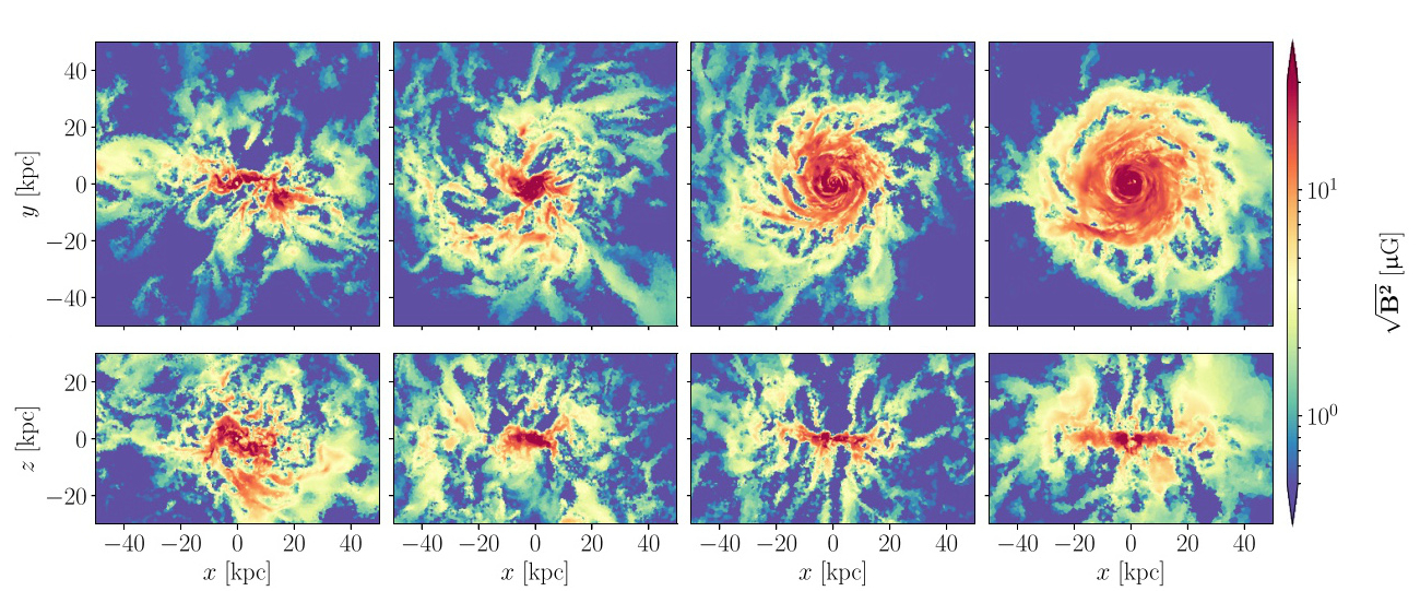
One exception to the Lagrangian models is the work of Rodenbeck & Schleicher 2016, who performed a grid simulation of a galaxy merger, using a simplified model without stellar feedback or a collisionless component. They found that the enhancement of the magnetic field is particularly pronounced in the central regions of the galaxy.
16.2 Magnetization of the CGM by outflows
Galactic outflows are fundamental in any theory of galaxy evolution. In starburst and dwarf galaxies they are powered by stellar feedback (Zhang 2018, e.g.,), while a few galaxies host AGN-powered winds (Fabian 2012, Kormendy & Ho 2013, Martin 1998, Veilleux et al. 2005). Recent work has indicated that, in some cases, galactic winds can be driven by cosmic ray (CR) pressure (Hanasz et al. 2013, Girichidis et al. 2016). The material carried by these outflows can magnetize the CGM.
In a recent study, van de Voort et al. 2021 performed direct galaxy evolution simulations while resolving the magnetized CGM, as part of the Auriga project. They found that, while the CGM remained a high-beta plasma, magnetic fields can noticeably change its structure around galaxies, indirectly affecting numerous galactic processes. For instance, galactic outflows become more collimated, resulting in less efficient mixing between enriched and un-enriched gas. Outflow speeds are also reduced in the presence of magnetization, which means that more metals remain in the halo with respect to the un-magnetized situation. The overall structure of the CGM is smoother, due to the additional magnetic pressure.
Arámburo-García et al. 2021 studied the magnetization of halos by AGN and SN-driven outflows in the Illustris-TNG simulations. They found that both types of outflows contributed to the creation of over-magnetized bubbles, with the AGN-driven bubbles playing the dominant role.
16.3 The impact of the environment on the galactic dynamo
The interaction of the galaxy with the CGM can have a crucial impact on the development of a dynamo. The loss of helicity flux through a galactic wind or fountain can help avoid catastrophic quenching and sustain a dynamo for longer (see Section 8.1), eventually reaching higher values of the saturated field. However, winds can also interfere with the dynamo itself if they are acting within the dynamo-active region. On the other hand, a strong magnetic field can suppress the galactic outflow.
Whether we are considering inflows, outflows, or a galactic fountain, the galaxy is always embedded in a current system that affects the evolution of the dynamo. This is a non-trivial complication of the effective boundary conditions because the level of magnetization of the inflowing or outflowing gas is unknown, and the extent of these flows can be much larger than the virial radius of the galaxy.
17 CONCLUSIONS
After 70 years of inquiry into the possibility of dynamos in galaxies, several important questions can now be answered. In virtually all astrophysical settings, there is turbulence and this turbulence is always magnetized because of small-scale dynamo action. Dynamos also work in decaying and otherwise nonstationary turbulence and can produce equipartition-strength magnetic fields exponentially on a turbulent turnover timescale. This realization makes the question of cosmological seed magnetic fields for galaxies and galaxy clusters almost obsolete, because they would always be overpowered by small-scale dynamos that can operate very rapidly when the scales are sufficiently small. While primordial magnetic fields may still be present and interesting in their own rights, the simple idea of them being wound up to explain the bisymmetric spiral of nonaxisymmetric magnetic fields in some galaxies is essentially ruled out.
While global numerical simulations are now beginning to show the production of magnetic fields in galaxies, there remains a big uncertainty regarding the question of what actually produces large-scale dynamo action. Is it really the effect or some other mechanisms at play? In this review, we have outlined several known mechanisms that could produce large-scale magnetic fields, but this question remains a major research topic in the years to come. One reason behind this is that the problem of catastrophic quenching is still not fully resolved. Low-resolution simulations of relatively diffusive dynamos may have been promising in terms of field strength and structure, but so far they have not survived the test of higher resolution. It remains important to continue to investigate this. At the same time, it is important to open one’s mind and think about dynamos beyond just the immediate proximity of a galaxy. The interaction with the CGM may be of crucial importance, and not all of the different processes, which are important, may qualify as a dynamo.
[SUMMARY POINTS]
- 1.
Small-scale dynamos work in all turbulent astrophysical environments.
- 2.
Simulations suggest that the efficiency of large-scale dynamos decreases with increasing resolution, probably because magnetic helicity fluxes are still inefficient.
- 3.
The relevance of an effect dynamo in galaxies remains unclear.
- 4.
Modern numerical simulations of galactic magnetic fields tend to take the past evolution of and the interaction with the environment into account.
[FUTURE ISSUES]
- 1.
The problem of catastrophic quenching remains relevant and will need to be addressed in high-resolution models with realistic boundary conditions.
- 2.
Numerical codes of galaxy evolution should take special care of the accurate treatment of magnetic fields, especially on the solenoidality constraint, a problem that is accentuated through the subgrid modeling of star formation and feedback.
- 3.
The next generation of numerical models should make an effort to identify observables related to the galactic dynamo that go beyond the BSS/ASS signature in the RM of galaxies.
- 4.
Future numerical models will have to quantify the importance of dynamo action in different stages of a galaxy’s evolution.
DISCLOSURE STATEMENT
The authors are not aware of any affiliations, memberships, funding, or financial holdings that might be perceived as affecting the objectivity of this review.
ACKNOWLEDGMENTS
We thank Eve Ostriker for a detailed review of the manuscript and Rainer Beck, Oliver Gressel, Yik Ki (Jackie) Ma, Anvar Shukurov, and Kandaswamy Subramanian for constructive comments on an earlier draft. We acknowledge support for the Nordita program on “Magnetic field evolution in low density or strongly stratified plasmas” in May 2022, when part of this work was done. EN also acknowledges Interstellar Institute’s program ”With Two Eyes” and the Paris-Saclay University’s Institut Pascal for hosting fruitful discussions that nourished some ideas included in this work. We acknowledge very useful discussions with Fabio Del Sordo, Frederick Gent, Sergio Martin-Alvarez, and Jennifer West. EN acknowledges funding from the ERC Grant ”Interstellar” (Grant agreement 740120) and the Hellenic Foundation for Research and Innovation (Project number 224). This work was supported by the Swedish Research Council (Vetenskapsrådet, 2019-04234). Nordita is sponsored by Nordforsk. We acknowledge the allocation of computing resources provided by the Swedish National Allocations Committee at the Center for Parallel Computers at the Royal Institute of Technology in Stockholm and Linköping.
References
- Alves Batista et al. (2019) Alves Batista R, Saveliev A, de Gouveia Dal Pino EM. 2019. MNRAS 489(3):3836–3849
- Andrievsky et al. (2015) Andrievsky A, Brandenburg A, Noullez A, Zheligovsky V. 2015. Ap. J. 811:135
- Arámburo-García et al. (2021) Arámburo-García A, Bondarenko K, Boyarsky A, Nelson D, Pillepich A, Sokolenko A. 2021. MNRAS 505(4):5038–5057
- Backus (1958) Backus G. 1958. Ann. Phys. 4(4):372–447
- Balbus & Hawley (1991) Balbus SA, Hawley JF. 1991. Ap. J. 376:214
- Balsara & Kim (2004) Balsara DS, Kim J. 2004. Ap. J. 602(2):1079–1090
- Baryshnikova et al. (1987) Baryshnikova I, Shukurov A, Ruzmaikin A, Sokoloff DD. 1987. A&A 177:27–41
- Beck et al. (2013) Beck AM, Dolag K, Lesch H, Kronberg PP. 2013. MNRAS 435(4):3575–3586
- Beck et al. (2012) Beck AM, Lesch H, Dolag K, Kotarba H, Geng A, Stasyszyn FA. 2012. MNRAS 422(3):2152–2163
- Beck (2001) Beck R. 2001. SSR 99:243–260
- Beck (2012) Beck R. 2012. SSR 166(1-4):215–230
- Beck (2015a) Beck R. 2015a. AAPR 24:4
- Beck (2015b) Beck R. 2015b. A&A 578:A93
- Beck et al. (2020) Beck R, Berkhuijsen EM, Gießübel R, Mulcahy DD. 2020. A&A 633:A5
- Beck et al. (2015) Beck R, Bomans D, Colafrancesco S, Dettmar RJ, Ferrière K, et al. 2015. Structure, dynamical impact and origin of magnetic fields in nearby galaxies in the SKA era. In Advancing Astrophysics with the Square Kilometre Array
- Beck et al. (1996) Beck R, Brandenburg A, Moss D, Shukurov A, Sokoloff D. 1996. Annu. Rev. Astron. Astrophys. 34:155–206
- Beck et al. (2019) Beck R, Chamandy L, Elson E, Blackman EG. 2019. Galaxies 8(1):4
- Beck et al. (1994) Beck R, Poezd AD, Shukurov A, Sokoloff DD. 1994. A&A 289:94–100
- Beck & Wielebinski (2013) Beck R, Wielebinski R. 2013. Magnetic Fields in Galaxies. In Planets, Stars and Stellar Systems: Galactic Structure and Stellar Populations, eds. TD Oswalt, G Gilmore, vol. 5. Springer Science+Business Media Dordrecht, 641–723
- Bendre & Subramanian (2022) Bendre AB, Subramanian K. 2022. MNRAS 511(3):4454–4463
- Bennett et al. (2013) Bennett CL, Larson D, Weiland JL, Jarosik N, Hinshaw G, et al. 2013. Ap. J. Suppl. 208(2):20
- Bernet et al. (2008) Bernet ML, Miniati F, Lilly SJ, Kronberg PP, Dessauges-Zavadsky M. 2008. Nature 454(7202):302–304
- Blackman & Brandenburg (2002) Blackman EG, Brandenburg A. 2002. Ap. J. 579(1):359–373
- Blackman & Field (2000) Blackman EG, Field GB. 2000. Ap. J. 534(2):984–988
- Borlaff et al. (2021) Borlaff AS, Lopez-Rodriguez E, Beck R, Stepanov R, Ntormousi E, et al. 2021. Ap. J. 921(2):128
- Brackbill & Barnes (1980) Brackbill JU, Barnes DC. 1980. J. Comp. Phys. 35(3):426–430
- Brandenburg (2000) Brandenburg A. 2000. Phil. Trans. Roy. Soc. Lond. A 358:759–774
- Brandenburg (2001) Brandenburg A. 2001. Ap. J. 550(2):824–840
- Brandenburg (2005) Brandenburg A. 2005. Ap. J. 625:539–547
- Brandenburg (2010) Brandenburg A. 2010. MNRAS 401(1):347–354
- Brandenburg (2018) Brandenburg A. 2018. J. Plasma Phys. 84:735840404
- Brandenburg (2019) Brandenburg A. 2019. MNRAS 487:2673–2684
- Brandenburg & Brüggen (2020) Brandenburg A, Brüggen M. 2020. Ap. J. Lett. 896:L14
- Brandenburg & Chatterjee (2018) Brandenburg A, Chatterjee P. 2018. Astron. Nachr. 339:118–126
- Brandenburg et al. (2010) Brandenburg A, Chatterjee P, Del Sordo F, Hubbard A, Käpylä PJ, Rheinhardt M. 2010. Phys. Scripta 142:014028
- Brandenburg et al. (2002) Brandenburg A, Dobler W, Subramanian K. 2002. Astron. Nachr. 323(2):99–122
- Brandenburg et al. (1993) Brandenburg A, Donner KJ, Moss D, Shukurov A, Sokoloff DD, Tuominen I. 1993. A&A 271:36–50
- Brandenburg et al. (1992) Brandenburg A, Donner KJ, Moss D, Shukurov A, Sokolov DD, Tuominen I. 1992. A&A 259:453–461
- Brandenburg et al. (1996) Brandenburg A, Enqvist K, Olesen P. 1996. Phys. Rev. D 54(2):1291–1300
- Brandenburg et al. (2019) Brandenburg A, Kahniashvili T, Mandal S, Roper Pol A, Tevzadze AG, Vachaspati T. 2019. Phys. Rev. F 4:024608
- Brandenburg & Ntormousi (2022) Brandenburg A, Ntormousi E. 2022. MNRAS 513(2):2136–2151
- Brandenburg et al. (2008a) Brandenburg A, Rädler KH, Rheinhardt M, Käpylä PJ. 2008a. Ap. J. 676:740–751
- Brandenburg et al. (2008b) Brandenburg A, Rädler KH, Rheinhardt M, Subramanian K. 2008b. Ap. J. Lett. 687:L49–L52
- Brandenburg & Rempel (2019) Brandenburg A, Rempel M. 2019. Ap. J. 879:57
- Brandenburg & Scannapieco (2020) Brandenburg A, Scannapieco E. 2020. Ap. J. 889(1):55
- Brandenburg & Sokoloff (2002) Brandenburg A, Sokoloff D. 2002. Geophys. Astrophys. Fluid Dyn. 96(4):319–344
- Brandenburg & Stepanov (2014) Brandenburg A, Stepanov R. 2014. Ap. J. 786:91
- Brandenburg & Subramanian (2005a) Brandenburg A, Subramanian K. 2005a. Phys. Rep. 417:1–209
- Brandenburg & Subramanian (2005b) Brandenburg A, Subramanian K. 2005b. Astron. Nachr. 326(6):400–408
- Brandenburg et al. (1990) Brandenburg A, Tuominen I, Krause F. 1990. Geophys. Astrophys. Fluid Dyn. 50(1):95–112
- Brandenburg et al. (2022) Brandenburg A, Zhou H, Sharma R. 2022. MNRAS 518(3):3312–3325
- Brentjens & de Bruyn (2005) Brentjens MA, de Bruyn AG. 2005. A&A 441(3):1217–1228
- Broderick et al. (2012) Broderick AE, Chang P, Pfrommer C. 2012. Ap. J. 752(1):22
- Burn (1966) Burn BJ. 1966. MNRAS 133:67
- Carretti et al. (2022) Carretti E, Vacca V, O’Sullivan SP, Heald GH, Horellou C, et al. 2022. MNRAS 512(1):945–959
- Cattaneo & Hughes (1996) Cattaneo F, Hughes DW. 1996. Phys. Rev. E 54(5):R4532–R4535
- Cattaneo & Vainshtein (1991) Cattaneo F, Vainshtein SI. 1991. Ap. J. Lett. 376:L21
- Chamandy et al. (2015) Chamandy L, Shukurov A, Subramanian K. 2015. MNRAS 446:L6–L10
- Chamandy et al. (2013) Chamandy L, Subramanian K, Shukurov A. 2013. MNRAS 428:3569–3589
- Chandrasekhar (1956) Chandrasekhar S. 1956. Ap. J. 124:244
- Cowling (1933) Cowling TG. 1933. MNRAS 94:39–48
- Crutcher (2012) Crutcher RM. 2012. Annu. Rev. Astron. Astrophys. 50:29–63
- Davis & Greenstein (1951) Davis Leverett J, Greenstein JL. 1951. Ap. J. 114:206
- Dayal & Ferrara (2018) Dayal P, Ferrara A. 2018. Phys. Rep. 780:1–64
- Dedner et al. (2002) Dedner A, Kemm F, Kröner D, Munz CD, Schnitzer T, Wesenberg M. 2002. J. Comp. Phys. 175(2):645–673
- Dekel et al. (2009) Dekel A, Birnboim Y, Engel G, Freundlich J, Goerdt T, et al. 2009. Nature 457(7228):451–454
- Del Sordo et al. (2013) Del Sordo F, Guerrero G, Brandenburg A. 2013. MNRAS 429:1686–1694
- Devlen et al. (2013) Devlen E, Brandenburg A, Mitra D. 2013. MNRAS 432:1651–1657
- Dickey et al. (2022) Dickey JM, West J, Thomson AJM, Landecker TL, Bracco A, et al. 2022. Ap. J. 940(1):75
- Donner & Brandenburg (1990) Donner KJ, Brandenburg A. 1990. A&A 240(2):289–298
- Draine (2011) Draine BT. 2011. Physics of the Interstellar and Intergalactic Medium. Princeton: Princeton University Press
- Durrive & Langer (2015) Durrive JB, Langer M. 2015. MNRAS 453(1):345–356
- Elstner et al. (1995) Elstner D, Golla G, Rudiger G, Wielebinski R. 1995. A&A 297:77–82
- Elstner et al. (1990) Elstner D, Meinel R, Rüdiger G. 1990. Geophys. Astrophys. Fluid Dyn. 50(1):85–94
- Evans & Hawley (1988) Evans CR, Hawley JF. 1988. Ap. J. 332:659
- Fabian (2012) Fabian AC. 2012. Annu. Rev. Astron. Astrophys. 50:455–489
- Federrath et al. (2011) Federrath C, Sur S, Schleicher DRG, Banerjee R, Klessen RS. 2011. Ap. J. 731(1):62
- Ferrière (2020) Ferrière K. 2020. Plasma Phys. Controlled Fusion 62(1):014014
- Fletcher et al. (2004) Fletcher A, Berkhuijsen EM, Beck R, Shukurov A. 2004. A&A 414:53–67
- Galloway & Proctor (1992) Galloway DJ, Proctor MRE. 1992. Nature 356(6371):691–693
- Garaldi et al. (2021) Garaldi E, Pakmor R, Springel V. 2021. MNRAS 502(4):5726–5744
- Gent et al. (2021) Gent FA, Mac Low MM, Käpylä MJ, Singh NK. 2021. Ap. J. Lett. 910(2):L15
- Gent et al. (2013) Gent FA, Shukurov A, Sarson GR, Fletcher A, Mantere MJ. 2013. MNRAS 430:L40–L44
- Girichidis et al. (2016) Girichidis P, Naab T, Walch S, Hanasz M, Mac Low MM, et al. 2016. Ap. J. Lett. 816(2):L19
- Gnedin et al. (2000) Gnedin NY, Ferrara A, Zweibel EG. 2000. Ap. J. 539(2):505–516
- Golla & Hummel (1994) Golla G, Hummel E. 1994. A&A 284:777–792
- Grand et al. (2017) Grand RJJ, Gómez FA, Marinacci F, Pakmor R, Springel V, et al. 2017. MNRAS 467(1):179–207
- Grasso & Rubinstein (1995) Grasso D, Rubinstein HR. 1995. Astropart. Phys. 3(1):95–102
- Gressel et al. (2013) Gressel O, Bendre A, Elstner D. 2013. MNRAS 429(2):967–972
- Gressel & Elstner (2020) Gressel O, Elstner D. 2020. MNRAS 494(1):1180–1188
- Gressel et al. (2008a) Gressel O, Elstner D, Ziegler U, Rüdiger G. 2008a. A&A 486(3):L35–L38
- Gressel et al. (2008b) Gressel O, Ziegler U, Elstner D, Rüdiger G. 2008b. Astron. Nachr. 329(6):619
- Gruzinov & Diamond (1996) Gruzinov AV, Diamond PH. 1996. Phys. Plasmas 3(5):1853–1857
- Hall (1949) Hall JS. 1949. Science 109(2825):166–167
- Han (2017) Han JL. 2017. Annu. Rev. Astron. Astrophys. 55(1):111–157
- Hanasz et al. (2013) Hanasz M, Lesch H, Naab T, Gawryszczak A, Kowalik K, Wóltański D. 2013. Ap. J. Lett. 777(2):L38
- Hennebelle & Inutsuka (2019) Hennebelle P, Inutsuka Si. 2019. Frontiers Astron. Space Sci. 6:5
- Henriksen et al. (2018) Henriksen RN, Woodfinden A, Irwin JA. 2018. MNRAS 476(1):635–645
- Herzenberg (1958) Herzenberg A. 1958. Phil. Trans. Roy. Soc. Lond. Ser. A 250(986):543–583
- Hiltner (1949) Hiltner WA. 1949. Science 109(2825):165
- Hollins et al. (2022) Hollins JF, Sarson GR, Evirgen CC, Shukurov A, Fletcher A, Gent FA. 2022. Geophys. Astrophys. Fluid Dyn. 116(4):261–289
- Horellou & Fletcher (2014) Horellou C, Fletcher A. 2014. MNRAS 441(3):2049–2057
- Hosking & Schekochihin (2021) Hosking DN, Schekochihin AA. 2021. Phys. Rev. X 11(4):041005
- Hosking & Schekochihin (2022) Hosking DN, Schekochihin AA. 2022. arXiv e-prints :arXiv:2203.03573
- Hutschenreuter et al. (2022) Hutschenreuter S, Anderson CS, Betti S, Bower GC, Brown JA, et al. 2022. A&A 657:A43
- Jaffe et al. (2010) Jaffe TR, Leahy JP, Banday AJ, Leach SM, Lowe SR, Wilkinson A. 2010. MNRAS 401(2):1013–1028
- Jansson & Farrar (2012) Jansson R, Farrar GR. 2012. Ap. J. 757(1):14
- Ji et al. (1995) Ji H, Prager SC, Sarff JS. 1995. Phys. Rev. Lett. 74(15):2945–2948
- Kahniashvili et al. (2022) Kahniashvili T, Clarke E, Stepp J, Brandenburg A. 2022. Phys. Rev. Lett. 128(22):221301
- Kahniashvili et al. (2013) Kahniashvili T, Maravin Y, Natarajan A, Battaglia N, Tevzadze AG. 2013. Ap. J. 770(1):47
- Kamionkowski et al. (1997) Kamionkowski M, Kosowsky A, Stebbins A. 1997. Phys. Rev. Lett. 78(11):2058–2061
- Katz et al. (2019) Katz H, Martin-Alvarez S, Devriendt J, Slyz A, Kimm T. 2019. MNRAS 484(2):2620–2631
- Kazantsev (1968) Kazantsev AP. 1968. Sov. J. Exp. Theor. Phys. 26:1031
- Keinigs (1983) Keinigs RK. 1983. Physics of Fluids 26(9):2558–2560
- Kormendy & Ho (2013) Kormendy J, Ho LC. 2013. Annu. Rev. Astron. Astrophys. 51(1):511–653
- Korochkin et al. (2021) Korochkin A, Kalashev O, Neronov A, Semikoz D. 2021. Ap. J. 906(2):116
- Korpi et al. (1999) Korpi MJ, Brandenburg A, Shukurov A, Tuominen I, Nordlund Å. 1999. Ap. J. Lett. 514(2):L99–L102
- Kotarba et al. (2010) Kotarba H, Karl SJ, Naab T, Johansson PH, Dolag K, et al. 2010. Ap. J. 716(2):1438–1452
- Kraichnan (1976) Kraichnan RH. 1976. J. Fluid Mech. 75:657–676
- Krasheninnikova et al. (1989) Krasheninnikova I, Shukurov A, Ruzmaikin A, Sokolov D. 1989. A&A 213:19–28
- Krause & Rädler (1980) Krause F, Rädler KH. 1980. Mean-Field Magnetohydrodynamics and Dynamo Theory. Oxford: Pergamon Press
- Krause et al. (1989) Krause M, Beck R, Hummel E. 1989. A&A 217:17–30
- Krause et al. (2020) Krause M, Irwin J, Schmidt P, Stein Y, Miskolczi A, et al. 2020. A&A 639:A112
- Krause et al. (2006) Krause M, Wielebinski R, Dumke M. 2006. A&A 448(1):133–142
- Kronberg et al. (1992) Kronberg PP, Perry JJ, Zukowski ELH. 1992. Ap. J. 387:528
- Kulsrud & Anderson (1992) Kulsrud RM, Anderson SW. 1992. Ap. J. 396:606
- Kulsrud et al. (1997) Kulsrud RM, Cen R, Ostriker JP, Ryu D. 1997. Ap. J. 480(2):481–491
- Lopez-Rodriguez et al. (2022) Lopez-Rodriguez E, Clarke M, Shenoy S, Vacca W, Coude S, et al. 2022. Ap. J. 936(1):65
- Lowes & Wilkinson (1963) Lowes FJ, Wilkinson I. 1963. Nature 198(4886):1158–1160
- Mao et al. (2017) Mao SA, Carilli C, Gaensler BM, Wucknitz O, Keeton C, et al. 2017. Nature Astron. 1:621–626
- Marinacci & Vogelsberger (2016) Marinacci F, Vogelsberger M. 2016. MNRAS 456(1):L69–L73
- Martin (1998) Martin CL. 1998. Ap. J. 506(1):222–252
- Martin-Alvarez et al. (2021) Martin-Alvarez S, Katz H, Sijacki D, Devriendt J, Slyz A. 2021. MNRAS 504(2):2517–2534
- Martin-Alvarez et al. (2020) Martin-Alvarez S, Slyz A, Devriendt J, Gómez-Guijarro C. 2020. MNRAS 495(4):4475–4495
- Mocz et al. (2016) Mocz P, Pakmor R, Springel V, Vogelsberger M, Marinacci F, Hernquist L. 2016. MNRAS 463(1):477–488
- Moffatt & Proctor (1985) Moffatt HK, Proctor MRE. 1985. J. Fluid Mech. 154:493–507
- Mora-Partiarroyo et al. (2019) Mora-Partiarroyo SC, Krause M, Basu A, Beck R, Wiegert T, et al. 2019. A&A 632:A11
- Moss (1996) Moss D. 1996. A&A 315:63–70
- Moss et al. (1993) Moss D, Brandenburg A, Donner KJ, Thomasson M. 1993. Ap. J. 409:179
- Moss & Sokoloff (2008) Moss D, Sokoloff D. 2008. A&A 487(1):197–203
- Mtchedlidze et al. (2022) Mtchedlidze S, Domínguez-Fernández P, Du X, Brandenburg A, Kahniashvili T, et al. 2022. Ap. J. 929(2):127
- Naoz & Narayan (2013) Naoz S, Narayan R. 2013. Phys. Rev. Lett. 111(5):051303
- Nelson et al. (2020) Nelson D, Sharma P, Pillepich A, Springel V, Pakmor R, et al. 2020. MNRAS 498(2):2391–2414
- Neronov & Vovk (2010) Neronov A, Vovk I. 2010. Science 328:73
- Ntormousi et al. (2022) Ntormousi E, Del Sordo F, Cantiello M, Ferrara A. 2022. A&A 668:L6
- Ntormousi et al. (2020) Ntormousi E, Tassis K, Del Sordo F, Fragkoudi F, Pakmor R. 2020. A&A 641:A165
- Ôki et al. (1964) Ôki T, Fujimoto M, Hitotuyanagi Z. 1964. Prog. Theor. Phys. Suppl. 31:77–115
- Oppermann et al. (2015) Oppermann N, Junklewitz H, Greiner M, Enßlin TA, Akahori T, et al. 2015. A&A 575:A118
- Page et al. (2007) Page L, Hinshaw G, Komatsu E, Nolta MR, Spergel DN, et al. 2007. Ap. J. Suppl. 170(2):335–376
- Pakmor et al. (2017) Pakmor R, Gómez FA, Grand RJJ, Marinacci F, Simpson CM, et al. 2017. MNRAS 469(3):3185–3199
- Parker (1955) Parker EN. 1955. Ap. J. 122:293
- Parker (1971) Parker EN. 1971. Ap. J. 163:255–278
- Parker (1979) Parker EN. 1979. Cosmical Magnetic Fields: Their Origin and Their Activity. Oxford: Clarendon Press
- Parker (1992) Parker EN. 1992. Ap. J. 401:137
- Pattle et al. (2022) Pattle K, Fissel L, Tahani M, Liu T, Ntormousi E. 2022. Protostars and Planets VII, in press :arXiv:2203.11179
- Piddington (1964) Piddington JH. 1964. MNRAS 128:345
- Piontek & Ostriker (2007) Piontek RA, Ostriker EC. 2007. Ap. J. 663(1):183–203
- Poezd et al. (1993) Poezd A, Shukurov A, Sokoloff D. 1993. MNRAS 264:285–297
- Powell et al. (1999) Powell KG, Roe PL, Linde TJ, Gombosi TI, De Zeeuw DL. 1999. J. Comp. Phys. 154(2):284–309
- Prasad & Mangalam (2016) Prasad A, Mangalam A. 2016. Ap. J. 817(1):12
- Putman et al. (2012) Putman ME, Peek JEG, Joung MR. 2012. Annu. Rev. Astron. Astrophys. 50:491–529
- Rädler (1969) Rädler KH. 1969. Monats. Dt. Akad. Wiss 11:194–201
- Rees (1987) Rees MJ. 1987. QJRAS 28:197–206
- Rheinhardt & Brandenburg (2012) Rheinhardt M, Brandenburg A. 2012. Astron. Nachr. 333:71–77
- Rheinhardt et al. (2014) Rheinhardt M, Devlen E, Rädler KH, Brandenburg A. 2014. MNRAS 441:116–126
- Rieder & Teyssier (2016) Rieder M, Teyssier R. 2016. MNRAS 457(2):1722–1738
- Rieder & Teyssier (2017a) Rieder M, Teyssier R. 2017a. MNRAS 471(3):2674–2686
- Rieder & Teyssier (2017b) Rieder M, Teyssier R. 2017b. MNRAS 472(4):4368–4373
- Rincon (2021) Rincon F. 2021. Phys. Rev. Fluids 6(12):L121701
- Roberts (1972) Roberts GO. 1972. Phil. Trans. Roy. Soc. Lond. Ser. A 271(1216):411–454
- Rodenbeck & Schleicher (2016) Rodenbeck K, Schleicher DRG. 2016. A&A 593:A89
- Rodrigues et al. (2019) Rodrigues LFS, Chamandy L, Shukurov A, Baugh CM, Taylor AR. 2019. MNRAS 483(2):2424–2440
- Roettiger et al. (1999) Roettiger K, Stone JM, Burns JO. 1999. Ap. J. 518(2):594–602
- Rosswog & Price (2007) Rosswog S, Price D. 2007. MNRAS 379(3):915–931
- Ruzmaikin et al. (1988) Ruzmaikin A, Shukurov A, Sokoloff D. 1988. Magnetic Fields of Galaxies. Dordrecht: Kluwer
- Schekochihin et al. (2004) Schekochihin AA, Cowley SC, Taylor SF, Maron JL, McWilliams JC. 2004. Ap. J. 612(1):276–307
- Schober et al. (2012) Schober J, Schleicher D, Federrath C, Glover S, Klessen RS, Banerjee R. 2012. Ap. J. 754(2):99
- Schoeffler et al. (2016) Schoeffler KM, Loureiro NF, Fonseca RA, Silva LO. 2016. Phys. Plasmas 23(5):056304
- Schrinner et al. (2005) Schrinner M, Rädler KH, Schmitt D, Rheinhardt M, Christensen U. 2005. Astron. Nachr. 326:245–249
- Schrinner et al. (2007) Schrinner M, Rädler KH, Schmitt D, Rheinhardt M, Christensen UR. 2007. Geophys. Astrophys. Fluid Dyn. 101:81–116
- Segalovitz et al. (1976) Segalovitz A, Shane WW, de Bruyn AG. 1976. Nature 264:222–226
- Seljak & Zaldarriaga (1997) Seljak U, Zaldarriaga M. 1997. Phys. Rev. Lett. 78(11):2054–2057
- Seta & Beck (2019) Seta A, Beck R. 2019. Galaxies 7:45
- Seta et al. (2020) Seta A, Bushby PJ, Shukurov A, Wood TS. 2020. Phys. Rev. Fluids 5(4):043702
- Seta & Federrath (2022) Seta A, Federrath C. 2022. MNRAS 514(1):957–976
- Shukurov (1998) Shukurov A. 1998. MNRAS 299(1):L21–l24
- Shukurov (2000) Shukurov A. 2000. Global magnetic structures in spiral galaxies: Evidence for dynamo action. In Proceedings 232. WE-Heraeus Seminar, pp. 191-200, astro-ph/0012460, eds. EM Berkhuijsen, R Beck, RAM Walterbos
- Shukurov et al. (2019) Shukurov A, Rodrigues LFS, Bushby PJ, Hollins J, Rachen JP. 2019. A&A 623:A113
- Shukurov et al. (2006) Shukurov A, Sokoloff D, Subramanian K, Brandenburg A. 2006. A&A 448:L33–L36
- Shukurov & Subramanian (2022) Shukurov A, Subramanian K. 2022. Astrophysical Magnetic Fields: From Galaxies to the Early Universe. Cambridge: Cambridge University Press
- Simard et al. (2016) Simard C, Charbonneau P, Dubé C. 2016. Adv. Spa. Res. 58(8):1522–1537
- Sironi & Giannios (2014) Sironi L, Giannios D. 2014. Ap. J. 787(1):49
- Snodin et al. (2006) Snodin AP, Brandenburg A, Mee AJ, Shukurov A. 2006. MNRAS 373:643–652
- Sofue et al. (1986) Sofue Y, Fujimoto M, Wielebinski R. 1986. Annu. Rev. Astron. Astrophys. 24:459–497
- Sokoloff & Shukurov (1990) Sokoloff D, Shukurov A. 1990. Nature 347(6288):51–53
- Soward (1987) Soward AM. 1987. J. Fluid Mech. 180:267–295
- Squire & Bhattacharjee (2015) Squire J, Bhattacharjee A. 2015. Phys. Rev. Lett. 115(17):175003
- Steenbeck & Krause (1969) Steenbeck M, Krause F. 1969. Astron. Nachr. 291:49–84
- Steenbeck et al. (1966) Steenbeck M, Krause F, Rädler KH. 1966. Zeitschr. Naturforsch. A 21:369
- Stein et al. (2019) Stein Y, Dettmar RJ, Weżgowiec M, Irwin J, Beck R, et al. 2019. A&A 632:A13
- Steinwandel et al. (2019) Steinwandel UP, Beck MC, Arth A, Dolag K, Moster BP, Nielaba P. 2019. MNRAS 483(1):1008–1028
- Stix (1975) Stix M. 1975. A&A 42(1):85–89
- Subramanian (2016) Subramanian K. 2016. RPPh 79(7):076901
- Subramanian & Brandenburg (2014) Subramanian K, Brandenburg A. 2014. MNRAS 445:2930–2940
- Subramanian et al. (1994) Subramanian K, Narasimha D, Chitre SM. 1994. MNRAS 271:L15
- Sun et al. (2008) Sun XH, Reich W, Waelkens A, Enßlin TA. 2008. A&A 477(2):573–592
- Sur et al. (2012) Sur S, Federrath C, Schleicher DRG, Banerjee R, Klessen RS. 2012. MNRAS 423(4):3148–3162
- Sur et al. (2010) Sur S, Schleicher DRG, Banerjee R, Federrath C, Klessen RS. 2010. Ap. J. Lett. 721(2):L134–L138
- Tabatabaei et al. (2008) Tabatabaei FS, Krause M, Fletcher A, Beck R. 2008. A&A 490(3):1005–1017
- Tassis et al. (2018) Tassis K, Ramaprakash AN, Readhead ACS, Potter SB, Wehus IK, et al. 2018. arXiv:1810.05652
- Terral & Ferrière (2017) Terral P, Ferrière K. 2017. A&A 600:A29
- Tosa & Fujimoto (1978) Tosa M, Fujimoto M. 1978. PASJ 30:315–326
- Tricco et al. (2016) Tricco TS, Price DJ, Federrath C. 2016. MNRAS 461(2):1260–1275
- Tüllmann et al. (2000) Tüllmann R, Dettmar RJ, Soida M, Urbanik M, Rossa J. 2000. A&A 364:L36–L41
- Vainshtein & Cattaneo (1992) Vainshtein SI, Cattaneo F. 1992. Ap. J. 393:165
- Vainshtein & Ruzmaikin (1971) Vainshtein SI, Ruzmaikin AA. 1971. AZh 48:902
- van de Voort et al. (2021) van de Voort F, Bieri R, Pakmor R, Gómez FA, Grand RJJ, Marinacci F. 2021. MNRAS 501(4):4888–4902
- Vazza et al. (2017) Vazza F, Brüggen M, Gheller C, Hackstein S, Wittor D, Hinz PM. 2017. Class. Quantum Grav. 34(23):234001
- Vazza et al. (2015) Vazza F, Ferrari C, Brüggen M, Bonafede A, Gheller C, Wang P. 2015. A&A 580:A119
- Veilleux et al. (2005) Veilleux S, Cecil G, Bland-Hawthorn J. 2005. Annu. Rev. Astron. Astrophys. 43(1):769–826
- Vishniac & Brandenburg (1997) Vishniac ET, Brandenburg A. 1997. Ap. J. 475:263–274
- Vishniac & Cho (2001) Vishniac ET, Cho J. 2001. Ap. J. 550(2):752–760
- Vishniac & Shapovalov (2014) Vishniac ET, Shapovalov D. 2014. Ap. J. 780(2):144
- Volegova & Stepanov (2010) Volegova AA, Stepanov RA. 2010. Sov. J. Exp. Theor. Phys. Lett. 90(10):637–641
- von Rekowski et al. (2003) von Rekowski B, Brandenburg A, Dobler W, Dobler W, Shukurov A. 2003. A&A 398:825–844
- Wang & Abel (2009) Wang P, Abel T. 2009. Ap. J. 696(1):96–109
- Warnecke et al. (2018) Warnecke J, Rheinhardt M, Tuomisto S, Käpylä PJ, Käpylä MJ, Brandenburg A. 2018. A&A 609:A51
- Weibel (1959) Weibel ES. 1959. Phys. Rev. Lett. 2(3):83–84
- West et al. (2020) West JL, Henriksen RN, Ferrière K, Woodfinden A, Jaffe T, et al. 2020. MNRAS 499(3):3673–3689
- White & Rees (1978) White SDM, Rees MJ. 1978. MNRAS 183:341–358
- Whittingham et al. (2021) Whittingham J, Sparre M, Pfrommer C, Pakmor R. 2021. MNRAS 506(1):229–255
- Widrow (2002) Widrow LM. 2002. Rev. Mod. Phys. 74(3):775–823
- Willis (2012) Willis AP. 2012. Phys. Rev. Lett. 109(25):251101
- Xu et al. (2019) Xu S, Garain SK, Balsara DS, Lazarian A. 2019. Ap. J. 872(1):62
- Xu & Lazarian (2016) Xu S, Lazarian A. 2016. Ap. J. 833(2):215
- Xu & Lazarian (2020) Xu S, Lazarian A. 2020. Ap. J. 899(2):115
- Xu & Lazarian (2021) Xu S, Lazarian A. 2021. Rev. Mod. Plasma Phys. 5(1):2
- Yousef et al. (2008) Yousef TA, Heinemann T, Schekochihin AA, Kleeorin N, Rogachevskii I, et al. 2008. PhRvL 100:184501
- Zeldovich et al. (1990) Zeldovich YB, Ruzmaikin AA, Sokoloff DD. 1990. The almighty chance. Singapore: World Scientific Publication
- Zhang (2018) Zhang D. 2018. Galaxies 6(4):114
- Zhou & Blackman (2021) Zhou H, Blackman EG. 2021. MNRAS 507(4):5732–5746
- Zhou et al. (2018) Zhou H, Blackman EG, Chamandy L. 2018. J. Plasma Phys. 84(3):735840302