A complete measurement of a black-hole recoil through higher-order gravitational-wave modes
Abstract
General relativity predicts that gravitational waves (GWs) carry linear momentum. Consequently, the remnant black hole of a black-hole merger can inherit a recoil velocity or “kick” of crucial implications in, e.g., black-hole formation scenarios. While the kick magnitude is determined by the mass ratio and spins of the source, estimating its direction requires a measurement of the two orientation angles of the source. While the orbital inclination angle is commonly reported in GW observations, the scientific potential of the azimuthal one has not been exploited to date. We show how the presence of more than one GW emission mode allows one to constrain this angle and, consequently, the kick direction of a real GW event. We analyse the GW190412 signal, which contains higher-order modes, with a numerical-relativity surrogate waveform model for black-hole mergers. We rule out kick magnitudes below the typical escape velocity of dense globular clusters km/s with a Bayes Factor of (or probability). The kick forms angles with the orbital angular momentum defined at a reference time before merger (with denoting the system mass in geometric units), with the line-of-sight. The projections of the kick and line-of-sight onto the orbital plane form an angle . All quantities are quoted at a credible level. Finally, by analyzing numerically simulated signals, we show that recoils can be estimated in an unbiased way using the NRSur7dq4 waveform model. We briefly discuss the potential application of this type of measurement for multi-messenger observations of black-hole mergers occurring in Active Galactic Nuclei.
I Introduction
Gravitational waves (GWs) carry linear momentum away from their sources (Misner et al. 1973) and asymmetric black-hole (BBH) mergers emit GWs in an anisotropic way. This causes a net emission of linear momentum that makes the final black hole (BH) acquire a recoil velocity (Thorne 1980; Fitchett 1983; Maggiore 2008; Gonzalez et al. 2007a; Herrmann et al. 2007; Koppitz et al. 2007; Sundararajan et al. 2010; Lousto and Zlochower 2011; Calderón Bustillo et al. 2018a), or kick, that in the most extreme cases can reach km/s (Campanelli et al. 2007; Gonzalez et al. 2007b; Bruegmann et al. 2008; Healy et al. 2009; Sperhake et al. 2020; Lousto and Zlochower 2011; Lousto and Zlochower 2013; Lousto et al. 2012). Such speeds can expel the remnant BH from their host environments preventing them from taking part in subsequent mergers and, therefore, from contributing to hierarchical BH formation mechanisms (Gerosa and Fishbach 2021). This has crucial astrophysical consequences as, e.g., such scenarios can explain the formation of supermassive BHs Volonteri et al. 2003; Volonteri 2010; Sakurai et al. 2017. Due to its paramount importance in BH formation, much work has been devoted towards estimating the kick magnitude of the remnant BHs of the GW events observed by Advanced LIGO (Aasi et al. 2015) and Advanced Virgo (Acernese et al. 2015) (Calderón Bustillo et al. 2018a; Varma et al. 2020; Abbott et al. 2020a; Varma et al. 2022a; Mahapatra et al. 2021a; Islam et al. 2023). The kick magnitude, together with its direction in the source frame, is determined by the mass ratio and spins of the merging BHs Campanelli et al. 2007; Gonzalez et al. 2007b; Bruegmann et al. 2008; Healy et al. 2009; Lousto and Zlochower 2011; Lousto and Zlochower 2013, with the spin relative orientations playing a particularly important role. Estimating these, however, is intrinsically challenging (Pürrer et al. 2016; Biscoveanu et al. 2021). Consequently, only three of the events detected to date (Abbott et al. 2019; Nitz et al. 2019; Venumadhav et al. 2020; Nitz et al. 2020; Abbott et al. 2021; Abbott et al. 2023a; Nitz et al. 2021; Nitz et al. 2023; Olsen et al. 2022), namely GW190814 (Mahapatra et al. 2021b), GW191109_010717 Islam et al. 2023 and GW200129_065458 (Varma et al. 2022a) (GW200129 hereafter), have allowed for an informative estimation of the recoil magnitude. Estimating the recoil direction with respect to the observer requires, in addition, an estimate of the two angles characterising the Earth’s location on the binary’s sky, which can be conversely understood as the BBH orientation w.r.t. the observer. We can access such information through the gravitational-wave mode content of the signal, as we outline next.

II Methods
II.1 The source frame and the orientation angles
The GW emission from a BBH can be described as a superposition of GW modes multiplied by spin(-2)-weighted spherical harmonics as (Goldberg et al. 1967; Blanchet 2024):
| (1) |
Here, denotes the intrinsic parameters (masses and spins) of the source. The parameter denotes the polar angle formed between the line-of-sight (LOS) and the (instantaneous) Newtonian orbital angular momentum , normal to the orbital plane defined at a given reference time during the BBH evolution. The value denotes a “face-on” observer while denotes an “edge-on” observer located on the orbital plane. The angle denotes the azimuthal angle of the observer, i.e., the angle formed by the projection of the line-of-sight onto the orbital plane and some preferential axis (Calderón Bustillo et al. 2018a) on it, which is commonly chosen11
1
We note that waveform models used within the LIGO, Virgo and KAGRA (LVK) Collaborations, implemented within the software LALSuite (LIGO Scientific Collaboration 2018), use a definition for the azimuthal angle . (See phiRef or in (Schmidt et al. 2017).) as the vector pointing from the lighter to the heavier BH (Schmidt et al. 2017).
II.2 Characterising the kick direction and re-defining the azimuthal angle
Within the above frame, the final BH kick can be characterised by its magnitude and the angles that it forms with and (See Fig. 1). Using the kick and the LOS, we can compute two more “observer-related” angles: the angle subtended between them and the angle formed by their projections on the orbital plane.
BBHs with spins (anti-)aligned with display a constantly oriented orbital plane. In this case, although is time-independent, clearly depends on . This partly motivates the latter to be systematically treated as a sort of “nuisance” parameter not reported in GW catalogues, commonly referred to as “coalescence phase”. The angle , however, provides a time-independent and more astrophysically motivated re-definition of the azimuthal location of the observer Calderón Bustillo et al. 2018a which, in the following, we will use to characterise both the source orientation and the kick direction.
Finally, for generically spinning BBHs, spin-orbit coupling causes to precess around the total angular momentum Apostolatos et al. 199422
2
Throughout this work, whenever is needed, we compute from the component spin vectors and orbital frequency up to 3.5 post-Newtonian order Bohé et al. 2013; Blanchet 2024, including spin-orbit effects.. This leads to a time-dependent orientation of the orbital plane, and . In this situation, it is common to replace the inclination angle by the angle Farr et al. 2014 formed between the LOS and the almost-conserved direction of (see Fig. 1). Analogously, we can replace by the angle formed between the projections of the LOS and onto the plane normal to .
II.3 Reading the kick and orientation angles from gravitational waves: GW200129 and GW190412
The spherical harmonics can be decomposed into amplitude and phase terms as . This shows that while controls the amplitude of each mode, determines the relative phase with which these modes interact, dramatically impacting the morphology, (i.e. the frequency content) of the observed signal (Calderón Bustillo et al. 2020). 33 3 Strictly, one needs either orbital precession or the observation of a higher-mode with odd- –suppressed for equal-mass BBHs– which leads to a non-periodic signal as a function of . For instance, the observation of e.g. a mode in an equal-mass non-precessing binary would lead to a bi-modal distribution for due to the periodicity of the signal as a function of .. Consequently, should be measurable if two modes with distinct frequency content are observed in the signal. This, however, requires the observation of either a precessing and/or unequal-mass BBH with non-zero inclination, which is challenging
First, the BBH emission is vastly dominated by the so-called “quadrupole” modes while further modes, known as higher-order modes (HMs), only contribute significantly for asymmetric sources with orientations . Second, while the joint observation of both dominant modes permits the estimation of for precessing sources O’Shaughnessy et al. 2013, these are however related by for non-precessing ones, reducing the impact of to a trivial phase shift Blanchet 2024; Harry et al. 2016; Harry et al. 2018 that prevents its measurement. Therefore, for non-precessing cases we can only measure through the observation of HMs with , which requires unequal-mass sources that are not face-on/off.
In addition, detecting these types of signals is nowadays very challenging. First, signals from highly inclined systems are weaker than those emitted face-on, reducing the chance of detection. Second, current matched-filter searches only target the quadrupole modes of non-precessing BBHs, reducing our sensitivity towards HM-rich or precessing signals (Capano et al. 2014; Varma et al. 2014; Calderón Bustillo et al. 2017; Harry et al. 2016; Harry et al. 2018; Calderón Bustillo et al. 2018b; Chandra et al. 2020; Chandra et al. 2022; Schmidt et al. 2024a; Schmidt et al. 2024b).
Despite this, the LVK confidently observed three such signals during its third observing run. First, GW200129 (Abbott et al. 2023a) displays signatures of precession (Hannam et al. 2022), allowing for an informative estimation of the kick magnitude km/s (Varma et al. 2022a) and, although not emphasised, a certain characterisation of the kick direction (see their Fig. 3). The interpretation of GW200129, however, has been challenged by Payne et al. 2022, due to potential data-quality issues in the Livingston detector44 4 See however Macas et al. 2024.. Second, while GW190814 Abbott et al. 2020b contains HMs and enabled a kick-magnitude measurement Mahapatra et al. 2021b, its mass ratio exceeds the limits of existing waveform models directly calibrated to numerical simulations Varma et al. 2019a; Varma et al. 2019b, presumably needed to accurately estimate the kick direction. With this, we focus on the BBH event GW190412 (Abbott et al. 2020c) which, while showing no signatures of precession, has a mass-ratio and orbital inclination at the credible level. Consequently, GW190412 contains measurable HMs Roy et al. 2021, making it a suitable candidate for constraining the kick direction.
II.4 Parameter inference
We perform Bayesian parameter inference on 4 seconds of publicly available data from the two Advanced LIGO and the Advanced Virgo detectors around the time of GW190412, sampled at 2048 Hz, using the software Parallel Bilby Ashton et al. 2019; Smith et al. 2020. We compare GW190412 with the state-of-the-art BBH waveform template model NRSur7dq4 (Varma et al. 2019a), which includes the impact of orbital precession and HMs.
Our waveform model choice is motivated by two factors.
First, unlike alternative models for precessing BBHs used by the LVK for the analysis of this signal (namely IMRPhenomPv3HM (Khan et al. 2020) and SEOBNRv4PHM (Ossokine et al. 2020; Pan et al. 2014; Babak et al. 2017)), NRSur7dq4 is directly fitted to generically precessing numerical relativity (NR) simulations. In particular, on the one hand, the first two models reproduce the impact of precession through post-Newtonian Schmidt et al. 2012; Hannam et al. 2014 and effective-one-body approximations Buonanno et al. 2003 that break down near the merger stage Hannam et al. 2022; Ossokine et al. 2020. On the other hand, and more crucial for this study, the relative phase of the individual modes of these models is not calibrated to NR during the merger-ringdown stage, which can lead to biased estimations of both the kick magnitude, direction and azimuthal angle Borchers and Ohme 2023. Second, the associated model NRSur7dq4Remnant (Varma et al. 2019a) provides accurate estimations of the magnitude and direction of the kick given the BBH parameters. As a shortcoming, the limited time length of the waveforms generated by NRSur7dq4 prevents the analysis of the full signal. Consistently with the re-analysis of GW190412 done by Islam et al. 2021 using NRSur7dq4, we start our analysis at a frequency Hz, instead of the value Hz used by the LVK. Consistently with Islam et al. 2021, despite the missing information in the Hz band 55
5
Also, some higher-order modes in our waveforms, such as the or will start above 40 Hz. Using the IMRPhenomXPHM waveform model Pratten et al. 2021, we have checked that the corresponding missing information – in terms of signal-to-noise ratio – does not impact our results, consistently with Islam et al. 2021., we obtain parameter estimates consistent with those of the LVK, plus informative estimates of both the magnitude and direction of the kick.
We place uniform priors in the detector-frame masses, spin magnitudes, time-of arrival and signal polarisation, together with isotropic priors in spin and source orientation and a luminosity distance prior as in Abbott et al. 2020c; Abbott et al. 2016. We sample the likelihood on the parameter space using the nested sampler Dynesty (Speagle 2020) with 4096 live points 66
6
We do not marginalise over calibration uncertainty, as this is not expected to have a significant impact at the current detector sensitivity Vitale et al. 2012; Payne et al. 2020; Huang et al. 2022.
Finally, in order to show that the kick direction characterisation comes from the information encoded in the HMs, we also analyse GW190412 by removing HMs and/or precession from our templates. We report our results as median values together with symmetric 90% credible intervals.
III Results
III.1 Visualising GW190412 and the kick impact
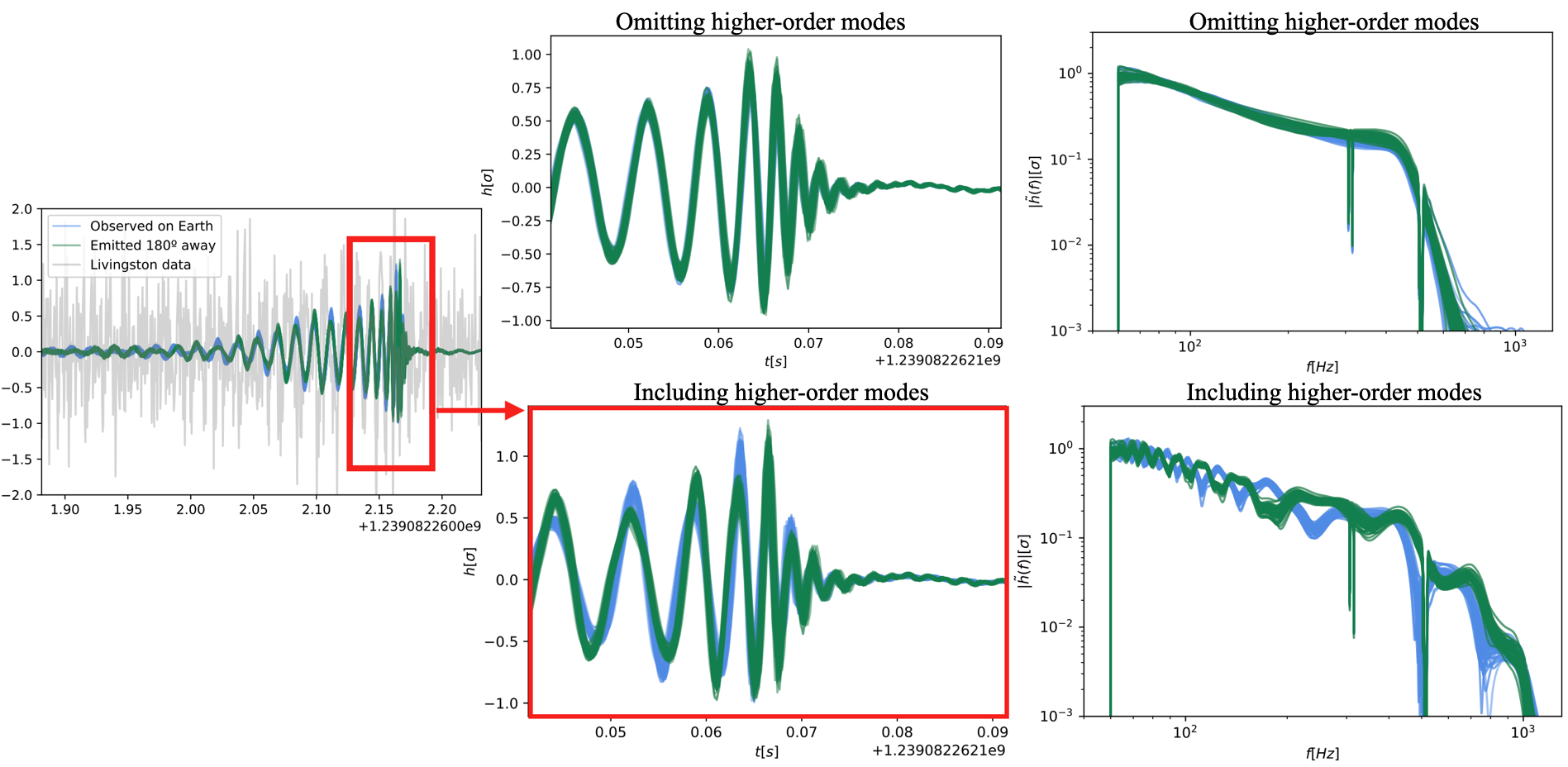
The left panel of Fig. 2 shows the whitened data from the Livingston detector at the time of GW190412 (grey) together with the 100 best-fitting templates (blue). In green, we show the corresponding signals observed in the opposite direction around the source, i.e., observed at . The bottom-central panel shows the last few cycles of these waveforms while the top-central panel shows the same waveforms, but with the HMs removed. While in the first case the two sets of signals clearly differ, therefore enabling measurement of and , these are almost identical when HMs are removed, preventing such measurements. Finally, the rightmost panels show these waveforms in the frequency domain. The bottom panel makes it obvious that the two waveforms show very different frequency content as a result of different interactions of the GW modes Calderón Bustillo et al. 2018a; Calderón Bustillo et al. 2020. Finally, the central and right bottom panels show that the kick direction is encoded in morphological waveform differences arising from the varying mode combinations in the recorded by different observers around the source Calderón Bustillo et al. 2018a; Calderón Bustillo et al. 2020, which vastly dominate putative Doppler shifts arising from the speed of the source relative to the observer Gerosa and Moore 2016.
III.2 Earth’s azimuthal angle around GW190412
The left panel of Fig. 3 shows in red the posterior distributions for inferred when both HMs and orbital precession are included in the analysis, estimated at a reference time before merger77
7
In geometric units, setting , with denoting the total mass of the binary in geometric units.. The prior probability is shown in black. The two remaining posteriors omit HMs, the circle-filled one omitting also precession. Ignoring HMs yields uninformative posteriors, as expected, while the inclusion of HMs leads to a clearly informative posterior, yielding 88
8
We note that when precession is considered, certain information on can be retrieved even if ignoring higher modes O’Shaughnessy et al. 2013. The reason is that while the modes are related by for non-precessing sources, and therefore have identical frequency content, such relation does not hold in general.. To highlight the time-dependence of , the filled histograms of the central panel show the posterior for compared to those obtained at and when orbital precession is omitted.
The empty histograms, instead, show the angles , computed on the orbital plane (solid lines), and , computed on the plane normal to (dashed). These two are coincident and time-independent in the absence of precession, providing a clear physical interpretation of the azimuthal angle. Finally, the right panel shows the same quantities as the central one, with precession included. Estimates for are more informative and stable for varying than those for , owing to the lower variation of as the system evolves. Both estimates become not only way more informative at – when the gravitational field is stronger Varma et al. 2022b; Varma et al. 2022a -- but also highly consistent99
9
After , spin measurements start to become unreliable in NR simulations Varma et al. 2019a.. This indicates that and are rather aligned near the merger, consistently with the lack of evidence for precession in GW1904121010
10
See Ref. Abbott et al. 2020c and Sec. III C.. In the following, we quote measurements using 1111
11
We note that while we directly sample the parameter space using this , we have checked that almost identical posterior distributions are obtained by sampling at a reference frequency of 60 Hz, and then evolving the corresponding spin and orientation angles as predicted by both NRSur7dq4 and post-Newtonian theory, which we use as a robustness test. For the spin evolution, we used the SpinTaylorT5 Ajith 2011; Riccardo Sturani 2021 scheme, and adapted the implementation in PESummary *[][inparticular; thispieceofwrapper\hrefhttps://git.ligo.org/lscsoft/pesummary/-/blob/543d4c70a3d8d35d58e21a85411815c729af2666/pesummary/gw/conversions/evolve.py.]Hoy2021:PESummary to make use of reference times instead of reference frequencies. The PESummary code makes use of the evolution functions from LALSuite (LIGO Scientific Collaboration 2018)..
III.3 The kick of GW190412
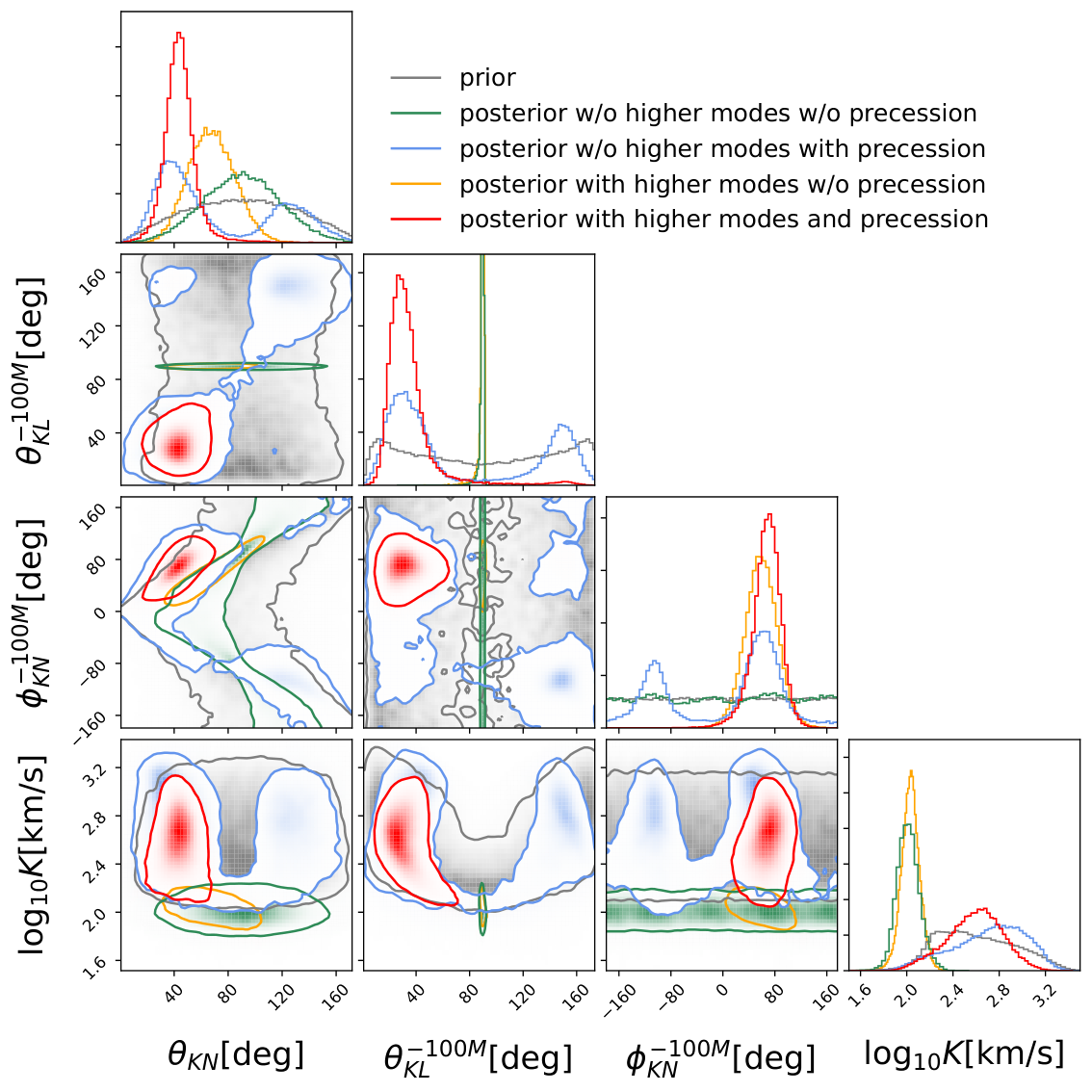
Fig. 4 shows, in red, the two-dimensional credible regions for the kick magnitude and the angles , and , together with the corresponding one-dimensional distributions. The prior distributions are shown in grey for the precessing case. While the kick magnitude is largely unconstrained, yielding km/s, the posterior significantly deviates from the prior, specially in the low-kick region. This allows us to rule out kicks below the typical escape velocity km/s of globular clusters and young-star clusters Holley-Bockelmann et al. 2008; Merritt et al. 2004; Antonini and Rasio 2016; Stoop et al. 2023a; Stoop et al. 2023b; Portegies Zwart et al. 2010; Mapelli et al. 2021, which are the best-motivated environments for GW190412 Gerosa et al. 20201212
12
This is based on the assumption that GW190412 formed hierarchically. However, Ref. Gerosa et al. 2020 also mentions that such environments are actually unlikely, precisely due to their low escape velocities. with a Bayes Factor of or, equivalently, probability (see Appendix I).
GW190412 contains rich information about the kick direction. First, the kick forms an angle with the LOS. Removing any combination of HMs and precession (green, red, magenta) leads to less informative or biased posteriors. Second, the prior for is symmetric around (i.e., with respect to the orbital plane) with peaks at and . This reflects the well-known fact that precessing sources preferentially lead to kicks out of the orbital plane Bruegmann et al. 2008; Lousto and Zlochower 2013; Varma et al. 2019c; O’Shaughnessy et al. 2013, but with no preference for shooting the final BH up or down, i.e., with a positive or negative projection of the kick onto . In contrast, the posterior distribution conclusively rules out a “negative projection”, indicating that the kick formed an angle with (i.e. with the orbital plane). Again, removing HMs leads to a less informative posterior that, in particular, barely distinguishes between the “upper” and “lower” branches. As expected, removing precession constrains the kick to the orbital plane. Third, we obtain an informative posterior for yielding . Similar to Fig. 3, removing both HMs and precession (green) yields a completely uninformative posterior while, if precession is included, a little information is retrieved thanks to the asymmetry between the modes (blue). Finally, we note that ignoring precession but including HMs (orange) yields results consistent with those including both effects. We understand this is consistent with the fact that orbital precession is not needed to explain GW190412 Abbott et al. 2020c1313
13
In fact, we obtain a Bayes factor of only 2.1 in favour of the precessing hypothesis over the non-precessing one..
Finally, while Varma et al. 2022a; Varma et al. 2019c suggest that some kick-direction estimates of NRSur7dq4Remnant may be inaccurate for kicks below km/s, we have thoroughly checked that our results are not impacted by this (see Appendix II).
IV Conclusions
Gravitational recoil is a strong-gravity effect of paramount importance in many astrophysical scenarios. Kick-magnitude estimates (Mahapatra et al. 2021b; Varma et al. 2022a) are crucial to understand the retention probability of BHs in their environments and, therefore, their ability to build hierarchical formation channels that can drive the formation of intermediate and supermassive BHs (Gerosa and Fishbach 2021). BHs recoiling through dense environments like Active Galactic Nuclei (AGN) can yield counterpart electromagnetic flares to GW signals (McKernan et al. 2019), as those recently proposed in Graham et al. 2020; Graham et al. 2023. If real, such multi-messenger observations can enable, e.g., independent estimates of the Hubble constant Mukherjee et al. 2020; Chen et al. 2022. Since the flare properties and observability depend on the direction of the kick w.r.t. both the host AGN and the observer Bellm et al. 2018; Graham et al. 2019, obtaining such information from GWs can help to assess the plausibility of the flare as a counterpart and as a probe of the AGN properties. For instance, if the kick is directed away from the observer, the corresponding flare will be obscured by the optically thick AGN disk 1414
14
We note that while this only makes use of , such estimate requires measurements of both the inclination and azimuth of the binary.. While there is no candidate electromagnetic counterpart to GW190412, we foresee the usage of the recoil direction to assess the plausibility of future candidates.
Our measurement requires that of the physically meaningful azimuthal angle of the observer around the source – misleadingly known as “coalescence phase” – that can be compared to the kick azimuthal angle . We hope that as gravitational-wave detectors and search techniques improve their respective sensitivities, increasing the number of events with HM content, this will become common practice. Finally, we note that the restriction to the quasi-circular case imposes constraints on the remnant kick magnitudes. Should GW190412 be consistent with an eccentric binary, larger kicks may be allowed Sperhake et al. 2020; Radia et al. 2021.
Appendix I Bayesian evidences for analyses using restricted kick-magnitude ranges
As discussed in the main text, when considering the full possible range of kick magnitudes, our posterior distribution for the kick magnitude largely follows the prior, leading to a fairly unconstrained kick magnitude. Even in this situation, however, we find that the data is informative enough to rule out small kicks below 50 km/s with high probability. In this Appendix, we describe the procedure followed to obtain this result.
Evaluating the probability of a non-zero kick
Given our priors on mass ratios and spins, the prior probability for a zero kick is exactly zero, which automatically yields a null posterior probability. This is astrophysically sensible, as the conditions required for null kicks are extremely restrictive. For instance, for the case of non-spinning binaries, the kick will only be zero if both black holes have exactly the same mass, which represents a sub-space of zero volume within all the possible mass ratios. In such scenario, however, it may be argued that the inference of a non-zero kick may just be driven by prior assumptions and not from information retrieved from the data.
In this situation, one can evaluate the need for a non-zero kick to explain the data in a prior-independent way. In particular, the relative probability for a signal model imposing zero and non-zero kicks can be obtained by simply performing two different parameter inference runs – the one presented in the main text and one imposing – and computing the ratio of respective Bayesian evidences, and , known as Bayes Factor . The kick magnitude, however, is not an explicit parameter of waveform models but an implicit one determined by the mass ratio and spins of the source, which makes cumbersome to perform the mentioned experiment. In this situation, it is well known that can be simply obtained through the Savage-Dickey density ratio Dickey 1971, equal to the ratio of the prior and posterior probabilities for evaluated at . However, since in our case both prior and posterior equal to zero (see the top panel of Fig. 5), such calculation can also be problematic.
Evaluating the probability for a kick above and below a finite value
In order to obtain robust results, we choose instead to compute the Bayes Factor , defined as the ratio of the evidences and respectively corresponding to analyses (or source models) restricted to kick magnitudes above and below a given threshold . This way, both prior and posterior are non-zero in the ranges of interest. As we show later, this can be simply obtained as
| (I.2) |
Above, denotes the posterior probability for marginalised over all other parameters while denotes the corresponding prior probability. These are respectively the grey and red distributions for shown in Fig. 4.
We show the mentioned distributions again in the top panel of Fig. 5, zooming in the region km/s, which was imperceptible in Fig. 4. First, it is rather obvious that the posterior deviates from the prior in that region, indicating that the data is indeed informative in the low-K end. Second, while the prior has support all the way to , the posterior shows negligible probability for km/s, which is the typical escape velocity of globular clusters and young-star clustersHolley-Bockelmann et al. 2008; Merritt et al. 2004; Antonini and Rasio 2016; Stoop et al. 2023a; Stoop et al. 2023b; Portegies Zwart et al. 2010; Mapelli et al. 2021. In other words, the data is informative enough to overcome the non-negligible prior probability for such low kicks. Using Eq. (I.2), we obtain . This is, a model restricted to km/s is times more probable given the data than a model restricted to km/s. Equivalently, km/s with probability.
The red line in the bottom panel of Fig. 5 shows as a function of the cutoff. First, we note that, as expected by looking at the top panel, increases for decreasing . The reason is that the ratio between the posterior and the prior probabilities for decreases for decreasing . This is, the data increasingly overcomes the (already small) preference of the prior for small kicks below as decreases. On the contrary, for instance, prior and posterior show the same probability for km/s (and, therefore, for km/s), thus yielding .
We note that the obtention of is potentially subject to large uncertainties given the small sample count in the low kick region. To estimate such uncertainty, we generate 500 random realisations of the prior and posterior distributions (a process known as bootstrapping) and compute for each of them. The blue region in the bottom panel of Fig. 5 shows the credible intervals of as a function of . The dashed blue shows median value. We obtain at the level or, equivalently, . As expected, uncertainties increase for decreasing , due to the decreasing number of posterior samples, which becomes null for km/s leading to somewhat artificial values . We may assume, however, that for such values the true lower end of the credible interval should be equal or larger than that for km/s, which yields .
Finally, we note that this study ignores the intrinsic error in the estimation of the kick arising in the actual numerical simulations due to, e.g., finite grid resolution. We show at the end of Appendix II that these do not seem to induce any significant systematic error in our analysis, or in those of significantly louder signals.
Derivation of Equation (I.2)
The posterior probability for source parameters given data is given by
| (I.3) |
Here, denotes the likelihood of the source parameters and denotes the prior probability for such parameters. Finally, the normalisation term denotes the Bayesian evidence, given by
| (I.4) |
where denotes the parameter space spanned by the parameters .
We can re-express as a function of a parameter of interest e.g., the kick magnitude parameter , as 1515 15 This assumes that: a) the function exists for all . b) is well behaved, i.e., not divergent, highly-oscillatory, fractal … We that note these conditions are also implicit to the obtention of the marginalised posterior distribution as that shown in Fig. 5, which has also been computed in works like Varma et al. 2022a; Abbott et al. 2020a.
| (I.5) |
Here, denotes the sub-parameter space spanned by the parameters satisfying . The second integral above is just the marginalised posterior probability for the kick magnitude –which we will denote by – times the evidence . This is represented in red in Figs. 4 and 5. The corresponding marginal likelihood can be obtained as
| (I.6) |
where denotes the prior on induced by the prior . The latter is represented in grey in Figs. 4 and 5 and is given by:
| (I.7) |
With this, we can re-express the evidence as
| (I.8) |
Evidence for restricted kick ranges
Let denote the prior for the kick magnitude of our analysis allowing for generic kicks. Next, we need to impose a new prior that corresponds to a restriction of our generic analysis to . To do this, we define as if – with a normalisation constant – and if .
The Bayesian evidence under the new prior is given by
| (I.9) |
Dividing and multiplying by the original prior , we can re-express the above as
| (I.10) |
which we can re-express as
| (I.11) |
With this, using our definition for , we can re-express Eq. (I.11) as simply
| (I.12) |
Finally, since the prior must satisfy , the normalisation constant given by
| (I.13) |
.
Analogously, it is easy to check that the Bayesian evidence for a model constrained to kicks is given by
| (I.14) |
with
| (I.15) |
.
With this, we arrive at the result presented in Eq. (I.2):
| (I.16) |
Appendix II Assessment of systematic errors of NRSur7dq4Remnant for low kick magnitudes
The package NRSur7dq4Remnant Varma et al. 2019a can provide accurate estimates of the magnitude and direction of black-hole recoils. However, the authors noted that, in some cases, direction estimates can carry errors above with respect to those coming from numerical relativity simulations. In particular, Fig. 7 in Ref. Varma et al. 2019a shows that such errors are more common when the kick magnitude is below km/s.
Since our posterior distribution for the kick magnitude shows non-negligible probability for km/s, it is reasonable to ask whether the mentioned errors have an impact in on our results, affecting their reliability and robustness. To check that this is not the case, we have conducted a series of tests that we describe next.
Systematic errors I: placing restrictions on the kick magnitude
Figure 6 shows our one- and two-dimensional posterior distributions for the kick angles of GW190412 (just like Fig. 4 in the main text) for the case of our full analysis (red) and for the cases where the kick magnitude is restricted to values above (blue) and below (green) 300 km/s. The estimate of is nearly identical in all cases. The estimate of the angle between the kick and the orbital angular momentum is consistent across the different experiments, with those including kicks above 300 km/s showing a very slight stronger preference for low values, i.e., for kicks more aligned with the orbital angular momentum. Far from reflecting any systematic error, this is just a consequence of the well-known fact that stronger kicks happen for strongly precessing sources (including superkicks), which tend to kick the final black hole away from the orbital plane. Finally, as a consequence of the previous two results, the estimates for are also consistent, with those allowing for larger kick magnitudes being more constrained.

Systematic errors II: aligned spins vs. random spin direction
Sources with spins (anti)-aligned with the orbital angular momentum have their kicks constrained below km/s Healy et al. 2014. Fig. 4 in the main text shows our kick-angle estimates for these sources, as well as those for our generic analysis, allowing for random spin directions. As discussed, the posterior distributions for , which is the only angle that can be fairly compared, are completely consistent. The distributions for , however, are necessarily inconsistent because aligned-spin systems have their kick constrained to the orbital plane, yielding a delta distribution at .
Systematic errors III: back-of-the envelope estimate
Fig. 3 in Ref. Varma et al. 2019c shows the error in the estimation of the angle between the true kick of validation NR simulations and those predicted by the surrogate models NRSur3dq8 and NRSur7dq2. These are respectively restricted to aligned-spin binaries up to and precessing binaries up to 1616
16
While the same figure is shown in Fig. 7 of Varma et al. 2019a for the case of NRSur7dq4, the much higher density of points therein prevents the “quantitative” study in the next paragraph. We therefore use the results in Varma et al. 2019c as a proxy.. As one can see therein, in some cases errors are above 10 deg, which is below our typical statistical uncertainties, with the vast majority of them being between 0.02 and 0.1 rad (0.22 and 5 deg). Furthermore, error values clearly accumulate at the low end of the mentioned interval. Importantly, it is also clear that large errors are more common for sources with kicks below 300 km/s, especially when these have aligned spin (purple dots therein).
To make a pessimistic estimate of the potential impact of large errors, we consider a scenario where all our cases below 300 km/s correspond to spin-aligned sources. With this, we count cases above and cases below such limit, indicating that, in this unrealistically pessimistic scenario, only of such cases would have errors above our typical statistical uncertainty. While we do not know the exact parameters of the validation sources used in the mentioned figure, we can ballpark that since cases with km/s represent of our posterior distribution, then roughly of our samples would typically suffer from potentially significant systematic errors. In any case, the test above shows that our results are robust against the discussed systematic errors.
Systematic errors IV: NR resolution
We study in detail the potential impact that errors in the estimations of the kick magnitudes arising from the finite resolution of NR simulations can have on our estimate of the probability that the GW190412 kick is below 50 km/s. We note that, unfortunately, we could not estimate this from the Fig. 3 in Ref. Varma et al. 2019c mentioned above or Fig. 7 in Varma et al. 2019a, as those do not report numerical errors for the kick magnitude a function of the kick magnitude itself. To tackle this, we compute the kick magnitude for all of the simulations available in the SXS catalogue for which the kick is below km/s, for the two highest levels of accuracy that are publicly available. Out of the 47 simulations we have studied, only 4 show differences larger than km/s. These cases show errors of , , and km/s, with the first two being clear outliers of a distribution where and of the cases are respectively below 3 km/s and 5 km/s. Moreover, Fig. 7 shows that the 4 mentioned simulations are outside the parameter space of GW190412, as these have either a mass ratio and/or an effective-spin parameter . We note that since not all of the waveforms used to train NRSur7dq4 are publicly available. We believe, however, such waveforms would be of at least equal quality (if not higher) than the ones we have analysed. For instance, we note that in all the mentioned outliers the maximum publicly available resolution level is Lev3, as compared to the maximum resolution of Lev6 available for many waveforms in the catalogue. This makes us confident that our qualitative conclusions about the kick magnitude of GW190412 should not be affected by the resolution-error budget of the NR waveforms used to train NRSur7dq4.
Finally, we note that Fig. 7 in Varma et al. 2019a shows that uncertainties in the kick direction due to NR resolution are comparable to those of those of the NRSur7dq4Remnant model itself, which we have already discussed.

Full Bayesian Analysis and Bayesian Priors
In addition to the purely systematic errors discussed above, in Ref. Varma et al. 2020, the authors tried to estimate the kick of selected BBH mergers simulated with NRSur7dq4 through a full Bayesian analysis. To this, the authors injected numerically simulated signals in simulated Gaussian detector noise and recovered them with the strategy followed here. In Fig. 4 therein, however, they observe that, for some cases where the kick is below 300 km/s, the estimate of the direction is significantly biased with respect to the true value. This happens even when the injected signal is extremely loud.
First, we note that such analysis is subject to several types of “errors” or “uncertainties”: first, the potential systematic errors discussed above and, second, that of Bayesian priors. In particular, we note that the impact of priors is inherent to any analysis and would just indicate that the effect produced by the kicks (or rather, by the source properties leading to such kicks) in the waveforms is not strong enough for to overcome prior assumptions. Therefore, the fact that parameter inference analyses fail to recover true values is not necessarily indicative of systematic errors.
Finally, we also note that there is a potentially worrying case where a strong bias is found in the kick direction, where the injected signal has a signal-to-noise ratio (SNR) of 66. In principle, for such high SNR, one may expect the data to be informative enough to overcome any prior assumptions. However, there is a chance that such bias may be due to an extreme Gaussian noise realisation. Nevertheless, we note that this corresponds to 1 out of 6 cases where the authors performed injections with kicks around or below 300 km/s. Moreover, if this is not sourced by an extreme noise realisation, this seems consistent with the fact that, as discussed in Test III above, large systematic errors above in the NRSur7dq4Remnant estimates are only found in a small fraction of the cases with kicks below 300 km/s (if one looks at the generic brown cases shown in Fig. 3 of Varma et al. 2019c, which seems roughly consistent with that for NRSur7dq4Remnant in Fig. 7 of Varma et al. 2019a).
Appendix III Bayesian parameter recovery of numerically simulated signals
| SXS code | ||||||
|---|---|---|---|---|---|---|
| SXS:BBH:1443 | 5.681 | 0.4079 | 0.7372 | 0.2365 | 0.0000 | |
| SXS:BBH:1156 | 4.387 | 0.4663 | 0.7677 | 0.3299 | 0.2719 | |
| SXS:BBH:0283 | 3.000 | 0.3000 | 0.2999 | 0.3000 | 0.0000 | |
| SXS:BBH:1937 | 4.000 | 0.4001 | 0.0001 | 0.3200 | 0.0000 | |
| SXS:BBH:1593 | 3.500 | 0.7213 | 0.7588 | 0.2531 | 0.6866 | |
| SXS:BBH:1805 | 3.415 | 0.4849 | 0.7130 | 0.3743 | 0.2215 | |
| SXS:BBH:1676 | 3.253 | 0.4856 | 0.4018 | 0.3841 | 0.2245 | |
| SXS:BBH:1410 | 4.000 | 0.4680 | 0.4647 | 0.2525 | 0.4000 |
| Parameter | True value | |
|---|---|---|
| RA | ||
| DEC | ||
| Polarisation angle | ||
| Geocentric time | ||

Finally, we have performed a full parameter inference study on numerically simulated signals to further confirm the robustness of our results. We have injected in zero-noise simulated numerical-relativity signals for sources with parameters roughly consistent with those of GW190412, all obtained from the SXS waveform catalog The SXS Collaboration; Boyle et al. 2019; Mroué et al. 2013; Chu et al. 2016; Varma et al. 2019d; Varma et al. 2019a. These include all modes up to and are extrapolated to null infinity using an polynomial Boyle et al. 2019. We recover these signals using the NRSur7dq4 waveform model, estimating the corresponding final parameters using the NRSur7dq4Remnant model. We use the same exact detector configuration, power-spectral densities and Bayesian priors as in the main text. Table 1 describes the intrinsic parameters of the numerical-relativity simulations we selected while Table 2 describes the chosen sky-location and polarisation. Three of the systems have aligned spins, while the other five are precessing. Our injections span a wide range of kick magnitudes and expand outside the mass-ratio training range of NRSur7dq4. The latter is motivated by the fact that the posterior distribution for this parameter for GW190412 peaks around , where the end of the training range sits. Also, we note that while the posterior for the secondary spin shows non-zero probability for – also surpassing the limits of the surrogate training region – such posterior is rather uninformative, and any systematics should not impact our results. In fact, we have checked that visually identical posterior distributions are obtained for all kick parameters of GW190412 if we restrict to . GW190412 has an intermediate source inclination of measured at a reference frequency of 20 Hz Abbott et al. 2020c. For the sake of completeness we have selected three different source inclinations rad specified at . We note that while and define different notions of inclination for precessing sources, the broad inclination range that our injections cover contains well those consistent with GW190412. Combining this choice of with a rather arbitrary choice of , our injections cover a reasonably wide range for the kick angles and . In addition, for each injection we have chosen two distances such that the SNR of the signals is 18 and 50, respectively, around and significantly above that of GW190412. The total detector-frame mass is set to be consistent with that of GW190412. We used the same sampling setting as in the main text, with 4096 live points.
Figure 8 shows the posterior distributions, together with the credible intervals and the corresponding true values for the kick parameters1717
17
We compute the true values by explicitly performing the corresponding momentum integral (see e.g. Gonzalez et al. 2007a) instead of reading them from the metadata of the simulations, as the latter corresponds to a coordinate velocity Boyle et al. 2019. As a general rule, the true values are always within the credible intervals even for SNRs of 50, way beyond that of GW190412. There are only two exceptions to this, out of the 144 posteriors we show. The first one corresponds to the posterior for obtained for the SXS:BBH:1156 case for the lowest inclination we consider, for both SNRs. This is, however, due to the extremely small prior probability for the true value. This is consistent with the fact that the posterior, while biased, moves towards the true value when we raise the SNR, following the peak of the likelihood. The same behaviour can be observed for the SXS:BBH:1937 cases with and . We note that this is something that all GW analysis are subject to independently of the accuracy of the waveform models and would therefore happen even if the NRSur7dq4 was infinitely accurate. The second case corresponds to the posterior for the SXS:BBH:1156 case for and , for which the true value is slightly away of the credible interval while being well inside it for the case. In this case, we have evidence this is caused by actual waveform systematics that make NRSur7dq4 waveforms with biased values of fit the SXS waveform better than predicted for the true injected parameters. In particular, we have checked that the posteriors for match well the restriction of those for to only high likelihood parameters. Nevertheless, we note that consistently with Islam et al. 2021 our results rule out an edge-on inclination for GW190412 and stress that its SNR is rather around 18, for which we obtained unbiased estimates.
We note that the analysis of aligned-spin cases, while unbiased, proved to be particularly challenging. The reason is that the null prior probability for aligned-spins made sampler convergence particularly cumbersome, requiring us to use significantly more aggressive sampler configurations with a larger number of parallel chains than the default ones we used for generic-spin cases 1818
18
In particular, for precessing cases we used 4096 live points, 2 parallel chains, (with rwalk) and , while for aligned-spin injections we performed analyses using both 8 and 10 parallel chains. The latter two analyses show consistent results, which makes us confident that the runs are well converged.. In fact, the analysis of these injections returned Bayes Factors of order favouring aligned spins, indicating indeed that the sampler would need to explore in detail the narrow aligned-spin region of the parameter space. In contrast, GW190412 returns a Bayes Factors of only 2.1 in favour of the aligned-spins, making us confident that such aggressive sampler settings are not needed to analyze it.
All in all, our results indicate that our analysis is not impacted by systematic errors coming from waveform modelling. Moreover, this would still be the case even if GW190412 had an SNR of 50, way beyond that of any GW observation to date.
Acknowledgements
We thank Nicolas Sanchis-Gual, Barry McKernan and Saavik Ford for their comments on the manuscript. We thank Sergei Ossokine and Nathan Johnson-McDaniel for their advice to perform parameter estimation at a given reference time and Vijay Varma for discussions on the importance of this choice. We also thank Angela Borchers for useful discussions regarding the accuracy of kick estimations of various waveform models. Finally, we thank Thomas Dent, Tjonnie Li and Titus Mömbacher for useful discussions. The analysed data and the corresponding power spectral densities are publicly available at the online Gravitational Wave Open Science Center (Abbott et al. 2023b). JCB is supported by a fellowship from “la Caixa” Foundation (ID100010434) and from the European Union’s Horizon2020 research and innovation programme under the Marie Skłodowska-Curie grant agreement No 847648. The fellowship code is LCF/BQ/PI20/11760016. JCB is also supported by the research grant PID2020-118635GB-I00 and by a Ramón y Cajal Fellowship RYC2022-036203-I from the Spain-Ministerio de Ciencia e Innovación. KC acknowledges the generous support provided through NSF grant numbers PHY-2207638, AST-2307147, PHY-2308886, and PHY-2309064. We acknowledge using the IUCAA LDG cluster Sarathi for the computational/numerical work. The authors acknowledge computational resources provided by the CIT cluster of the LIGO Laboratory and supported by National Science Foundation Grants PHY-0757058 and PHY0823459, and the support of the NSF CIT cluster for the provision of computational resources for our parameter inference runs. This material is based upon work supported by NSF’s LIGO Laboratory which is a major facility fully funded by the National Science Foundation. The authors acknowledge the use of computing facilities supported by grants from the Croucher Innovation Award from the Croucher Foundation Hong Kong. This research has made use of data or software obtained from the Gravitational Wave Open Science Center (gwosc.org), a service of the LIGO Scientific Collaboration, the Virgo Collaboration, and KAGRA. This material is based upon work supported by NSF’s LIGO Laboratory which is a major facility fully funded by the National Science Foundation, as well as the Science and Technology Facilities Council (STFC) of the United Kingdom, the Max-Planck-Society (MPS), and the State of Niedersachsen/Germany for support of the construction of Advanced LIGO and construction and operation of the GEO600 detector. Additional support for Advanced LIGO was provided by the Australian Research Council. Virgo is funded, through the European Gravitational Observatory (EGO), by the French Centre National de Recherche Scientifique (CNRS), the Italian Istituto Nazionale di Fisica Nucleare (INFN) and the Dutch Nikhef, with contributions by institutions from Belgium, Germany, Greece, Hungary, Ireland, Japan, Monaco, Poland, Portugal, Spain. KAGRA is supported by Ministry of Education, Culture, Sports, Science and Technology (MEXT), Japan Society for the Promotion of Science (JSPS) in Japan; National Research Foundation (NRF) and Ministry of Science and ICT (MSIT) in Korea; Academia Sinica (AS) and National Science and Technology Council (NSTC) in Taiwan. This manuscript has LIGO DCC number P2200332.
References
- Misner et al. (1973) C. W. Misner, K. S. Thorne, and J. A. Wheeler, Gravitation (W. H. Freeman, San Francisco, 1973).
- Thorne (1980) K. S. Thorne, Rev. Mod. Phys. 52, 299 (1980).
- Fitchett (1983) M. J. Fitchett, Mon. Not. Roy. Astron. Soc. 203, 1049 (1983).
- Maggiore (2008) M. Maggiore, Gravitational Waves: Volume 1: Theory and Experiments, Gravitational Waves (OUP Oxford, 2008).
- Gonzalez et al. (2007a) J. A. Gonzalez, U. Sperhake, B. Bruegmann, M. Hannam, and S. Husa, Phys. Rev. Lett. 98, 091101 (2007a), arXiv:gr-qc/0610154 [gr-qc] .
- Herrmann et al. (2007) F. Herrmann, I. Hinder, D. Shoemaker, P. Laguna, and R. A. Matzner, Astrophys.J. 661, 430 (2007), arXiv:gr-qc/0701143 [gr-qc] .
- Koppitz et al. (2007) M. Koppitz, D. Pollney, C. Reisswig, L. Rezzolla, J. Thornburg, et al., Phys.Rev.Lett. 99, 041102 (2007), arXiv:gr-qc/0701163 [gr-qc] .
- Sundararajan et al. (2010) P. A. Sundararajan, G. Khanna, and S. A. Hughes, Phys. Rev. D81, 104009 (2010), arXiv:1003.0485 [gr-qc] .
- Lousto and Zlochower (2011) C. O. Lousto and Y. Zlochower, Phys. Rev. Lett. 107, 231102 (2011), arXiv:1108.2009 [gr-qc] .
- Calderón Bustillo et al. (2018a) J. Calderón Bustillo, J. A. Clark, P. Laguna, and D. Shoemaker, Phys. Rev. Lett. 121, 191102 (2018a), arXiv:1806.11160 [gr-qc] .
- Campanelli et al. (2007) M. Campanelli, C. O. Lousto, Y. Zlochower, and D. Merritt, Phys. Rev. Lett. 98, 231102 (2007), arXiv:gr-qc/0702133 .
- Gonzalez et al. (2007b) J. A. Gonzalez, M. D. Hannam, U. Sperhake, B. Bruegmann, and S. Husa, Phys. Rev. Lett. 98, 231101 (2007b), arXiv:gr-qc/0702052 .
- Bruegmann et al. (2008) B. Bruegmann, J. A. Gonzalez, M. Hannam, S. Husa, and U. Sperhake, Phys. Rev. D77, 124047 (2008), arXiv:0707.0135 [gr-qc] .
- Healy et al. (2009) J. Healy, F. Herrmann, I. Hinder, D. M. Shoemaker, P. Laguna, and R. A. Matzner, Phys. Rev. Lett. 102, 041101 (2009), arXiv:0807.3292 [gr-qc] .
- Sperhake et al. (2020) U. Sperhake, R. Rosca-Mead, D. Gerosa, and E. Berti, Physical Review D 101, 10.1103/physrevd.101.024044 (2020).
- Lousto and Zlochower (2013) C. O. Lousto and Y. Zlochower, Phys. Rev. D87, 084027 (2013), arXiv:1211.7099 [gr-qc] .
- Lousto et al. (2012) C. O. Lousto, Y. Zlochower, M. Dotti, and M. Volonteri, Physical Review D 85, 10.1103/physrevd.85.084015 (2012).
- Gerosa and Fishbach (2021) D. Gerosa and M. Fishbach, Nature Astronomy 5, 749 (2021), arXiv:2105.03439 [astro-ph.HE] .
- Volonteri et al. (2003) M. Volonteri, F. Haardt, and P. Madau, The Astrophysical Journal 582, 559 (2003).
- Volonteri (2010) M. Volonteri, The Astronomy and Astrophysics Review 18, 279 (2010).
- Sakurai et al. (2017) Y. Sakurai, N. Yoshida, M. S. Fujii, and S. Hirano, Monthly Notices of the Royal Astronomical Society 472, 1677 (2017).
- Aasi et al. (2015) J. Aasi et al. (LIGO Scientific), Class. Quant. Grav. 32, 074001 (2015), arXiv:1411.4547 [gr-qc] .
- Acernese et al. (2015) F. Acernese et al. (VIRGO), Class. Quant. Grav. 32, 024001 (2015), arXiv:1408.3978 [gr-qc] .
- Varma et al. (2020) V. Varma, M. Isi, and S. Biscoveanu, Physical Review Letters 124, 10.1103/physrevlett.124.101104 (2020).
- Abbott et al. (2020a) R. Abbott et al. (LIGO Scientific, Virgo), Astrophys. J. Lett. 900, L13 (2020a), arXiv:2009.01190 [astro-ph.HE] .
- Varma et al. (2022a) V. Varma, S. Biscoveanu, T. Islam, F. H. Shaik, C.-J. Haster, M. Isi, W. M. Farr, S. E. Field, and S. Vitale, Physical Review Letters 128, 10.1103/physrevlett.128.191102 (2022a).
- Mahapatra et al. (2021a) P. Mahapatra, A. Gupta, M. Favata, K. G. Arun, and B. S. Sathyaprakash, The Astrophysical Journal Letters 918, L31 (2021a).
- Islam et al. (2023) T. Islam, A. Vajpeyi, F. H. Shaik, C.-J. Haster, V. Varma, S. E. Field, J. Lange, R. O’Shaughnessy, and R. Smith, Analysis of gwtc-3 with fully precessing numerical relativity surrogate models (2023), arXiv:2309.14473 .
- Pürrer et al. (2016) M. Pürrer, M. Hannam, and F. Ohme, Phys. Rev. D93, 084042 (2016), arXiv:1512.04955 [gr-qc] .
- Biscoveanu et al. (2021) S. Biscoveanu, M. Isi, V. Varma, and S. Vitale, Phys. Rev. D 104, 103018 (2021), arXiv:2106.06492 [gr-qc] .
- Abbott et al. (2019) B. P. Abbott et al. (LIGO Scientific, Virgo), Phys. Rev. X 9, 031040 (2019), arXiv:1811.12907 [astro-ph.HE] .
- Nitz et al. (2019) A. H. Nitz, C. Capano, A. B. Nielsen, S. Reyes, R. White, D. A. Brown, and B. Krishnan, Astrophys. J. 872, 195 (2019), arXiv:1811.01921 [gr-qc] .
- Venumadhav et al. (2020) T. Venumadhav, B. Zackay, J. Roulet, L. Dai, and M. Zaldarriaga, Phys. Rev. D 101, 083030 (2020), arXiv:1904.07214 [astro-ph.HE] .
- Nitz et al. (2020) A. H. Nitz, T. Dent, G. S. Davies, S. Kumar, C. D. Capano, I. Harry, S. Mozzon, L. Nuttall, A. Lundgren, and M. Tápai, Astrophys. J. 891, 123 (2020), arXiv:1910.05331 [astro-ph.HE] .
- Abbott et al. (2021) R. Abbott et al. (LIGO Scientific, Virgo), Phys. Rev. X 11, 021053 (2021), arXiv:2010.14527 [gr-qc] .
- Abbott et al. (2023a) R. Abbott et al., Physical Review X 13, 10.1103/physrevx.13.041039 (2023a).
- Nitz et al. (2021) A. H. Nitz, C. D. Capano, S. Kumar, Y.-F. Wang, S. Kastha, M. Schäfer, R. Dhurkunde, and M. Cabero, Astrophys. J. 922, 76 (2021), arXiv:2105.09151 [astro-ph.HE] .
- Nitz et al. (2023) A. H. Nitz, S. Kumar, S. Wang, Yi-Fan, S. Wu, M. Schäfer, R. Dhurkunde, and C. D. Capano, The Astrophysical Journal 946, 59 (2023).
- Olsen et al. (2022) S. Olsen, T. Venumadhav, J. Mushkin, J. Roulet, B. Zackay, and M. Zaldarriaga, Phys. Rev. D 106, 043009 (2022), arXiv:2201.02252 [astro-ph.HE] .
- Mahapatra et al. (2021b) P. Mahapatra, A. Gupta, M. Favata, K. G. Arun, and B. S. Sathyaprakash, The Astrophysical Journal Letters 918, L31 (2021b).
- Goldberg et al. (1967) J. N. Goldberg, A. J. MacFarlane, E. T. Newman, F. Rohrlich, and E. C. G. Sudarshan, J. Math. Phys. 8, 2155 (1967).
- Blanchet (2024) L. Blanchet, Living Reviews in Relativity 27, 10.1007/s41114-024-00050-z (2024).
- LIGO Scientific Collaboration (2018) LIGO Scientific Collaboration, LIGO Algorithm Library - LALSuite, free software (GPL) (2018).
- Schmidt et al. (2017) P. Schmidt, I. W. Harry, and H. P. Pfeiffer, (2017), arXiv:1703.01076 [gr-qc] .
- Apostolatos et al. (1994) T. A. Apostolatos, C. Cutler, G. J. Sussman, and K. S. Thorne, Phys.Rev. D49, 6274 (1994).
- Bohé et al. (2013) A. Bohé, S. Marsat, G. Faye, and L. Blanchet, Classical and Quantum Gravity 30, 075017 (2013).
- Farr et al. (2014) B. Farr, E. Ochsner, W. M. Farr, and R. O’Shaughnessy, Physical Review D 90, 10.1103/physrevd.90.024018 (2014).
- Calderón Bustillo et al. (2020) J. Calderón Bustillo, C. Evans, J. A. Clark, G. Kim, P. Laguna, and D. Shoemaker, Communications Physics 3, 176 (2020), arXiv:1906.01153 [gr-qc] .
- O’Shaughnessy et al. (2013) R. O’Shaughnessy, L. London, J. Healy, and D. Shoemaker, Physical Review D 87, 10.1103/physrevd.87.044038 (2013).
- Harry et al. (2016) I. Harry, S. Privitera, A. Bohé, and A. Buonanno, Phys. Rev. D94, 024012 (2016), arXiv:1603.02444 [gr-qc] .
- Harry et al. (2018) I. Harry, J. Calderón Bustillo, and A. Nitz, Phys. Rev. D97, 023004 (2018), arXiv:1709.09181 [gr-qc] .
- Capano et al. (2014) C. Capano, Y. Pan, and A. Buonanno, Phys.Rev. D89, 102003 (2014), arXiv:1311.1286 [gr-qc] .
- Varma et al. (2014) V. Varma, P. Ajith, S. Husa, J. C. Bustillo, M. Hannam, et al., Phys.Rev. D90, 124004 (2014), arXiv:1409.2349 [gr-qc] .
- Calderón Bustillo et al. (2017) J. Calderón Bustillo, P. Laguna, and D. Shoemaker, Phys. Rev. D95, 104038 (2017), arXiv:1612.02340 [gr-qc] .
- Calderón Bustillo et al. (2018b) J. Calderón Bustillo, F. Salemi, T. Dal Canton, and K. P. Jani, Phys. Rev. D97, 024016 (2018b), arXiv:1711.02009 [gr-qc] .
- Chandra et al. (2020) K. Chandra, V. Gayathri, J. C. Bustillo, and A. Pai, Phys. Rev. D 102, 044035 (2020), arXiv:2002.10666 [astro-ph.CO] .
- Chandra et al. (2022) K. Chandra, J. C. Bustillo, A. Pai, and I. Harry, Physical Review D 106, 10.1103/physrevd.106.123003 (2022).
- Schmidt et al. (2024a) S. Schmidt et al., Phys. Rev. D 110, 023038 (2024a), arXiv:2403.17186 [gr-qc] .
- Schmidt et al. (2024b) S. Schmidt et al., Phys. Rev. Lett. 133, 201401 (2024b), arXiv:2406.17832 [gr-qc] .
- Hannam et al. (2022) M. Hannam, C. Hoy, J. E. Thompson, S. Fairhurst, V. Raymond, M. Colleoni, D. Davis, H. Estellés, C.-J. Haster, A. Helmling-Cornell, S. Husa, D. Keitel, T. J. Massinger, A. Menéndez-Vázquez, K. Mogushi, S. Ossokine, E. Payne, G. Pratten, I. Romero-Shaw, J. Sadiq, P. Schmidt, R. Tenorio, R. Udall, J. Veitch, D. Williams, A. B. Yelikar, and A. Zimmerman, Nature 10.1038/s41586-022-05212-z (2022).
- Payne et al. (2022) E. Payne, S. Hourihane, J. Golomb, R. Udall, D. Davis, and K. Chatziioannou, Physical Review D 106, 10.1103/physrevd.106.104017 (2022).
- Macas et al. (2024) R. Macas, A. Lundgren, and G. Ashton, Physical Review D 109, 10.1103/physrevd.109.062006 (2024).
- Abbott et al. (2020b) R. Abbott et al., The Astrophysical Journal Letters 896, L44 (2020b).
- Varma et al. (2019a) V. Varma, S. E. Field, M. A. Scheel, J. Blackman, D. Gerosa, L. C. Stein, L. E. Kidder, and H. P. Pfeiffer, Physical Review Research 1, 10.1103/physrevresearch.1.033015 (2019a).
- Varma et al. (2019b) V. Varma, S. E. Field, M. A. Scheel, J. Blackman, L. E. Kidder, and H. P. Pfeiffer, Physical Review D 99, 10.1103/physrevd.99.064045 (2019b).
- Abbott et al. (2020c) R. Abbott et al., Physical Review D 102, 10.1103/physrevd.102.043015 (2020c).
- Roy et al. (2021) S. Roy, A. S. Sengupta, and K. G. Arun, Physical Review D 103, 10.1103/physrevd.103.064012 (2021).
- Ashton et al. (2019) G. Ashton et al., Astrophys. J. Suppl. 241, 27 (2019), arXiv:1811.02042 [astro-ph.IM] .
- Smith et al. (2020) R. J. E. Smith, G. Ashton, A. Vajpeyi, and C. Talbot, Mon. Not. Roy. Astron. Soc. 498, 4492 (2020), arXiv:1909.11873 [gr-qc] .
- Khan et al. (2020) S. Khan, F. Ohme, K. Chatziioannou, and M. Hannam, Physical Review D 101, 10.1103/physrevd.101.024056 (2020).
- Ossokine et al. (2020) S. Ossokine et al., Phys. Rev. D 102, 044055 (2020), arXiv:2004.09442 [gr-qc] .
- Pan et al. (2014) Y. Pan, A. Buonanno, A. Taracchini, L. E. Kidder, A. H. Mroue, H. P. Pfeiffer, M. A. Scheel, and B. Szilágyi, Phys. Rev. D89, 084006 (2014), arXiv:1307.6232 [gr-qc] .
- Babak et al. (2017) S. Babak, A. Taracchini, and A. Buonanno, Phys. Rev. D95, 024010 (2017), arXiv:1607.05661 [gr-qc] .
- Schmidt et al. (2012) P. Schmidt, M. Hannam, and S. Husa, Phys. Rev. D86, 104063 (2012), arXiv:1207.3088 [gr-qc] .
- Hannam et al. (2014) M. Hannam, P. Schmidt, A. Bohé, L. Haegel, S. Husa, F. Ohme, G. Pratten, and M. Pürrer, Phys. Rev. Lett. 113, 151101 (2014), arXiv:1308.3271 [gr-qc] .
- Buonanno et al. (2003) A. Buonanno, Y. Chen, and M. Vallisneri, Physical Review D 67, 10.1103/physrevd.67.104025 (2003).
- Borchers and Ohme (2023) A. Borchers and F. Ohme, Classical and Quantum Gravity 40, 095008 (2023).
- Islam et al. (2021) T. Islam, S. E. Field, C.-J. Haster, and R. Smith, Physical Review D 103, 10.1103/physrevd.103.104027 (2021).
- Pratten et al. (2021) G. Pratten, C. García-Quirós, M. Colleoni, A. Ramos-Buades, H. Estellés, M. Mateu-Lucena, R. Jaume, M. Haney, D. Keitel, J. E. Thompson, and S. Husa, Physical Review D 103, 10.1103/physrevd.103.104056 (2021).
- Abbott et al. (2016) B. P. Abbott et al., Physical Review Letters 116, 10.1103/physrevlett.116.241102 (2016).
- Speagle (2020) J. S. Speagle, Monthly Notices of the Royal Astronomical Society 493, 3132 (2020).
- Vitale et al. (2012) S. Vitale, W. Del Pozzo, T. G. F. Li, C. Van Den Broeck, I. Mandel, B. Aylott, and J. Veitch, Physical Review D 85, 10.1103/physrevd.85.064034 (2012).
- Payne et al. (2020) E. Payne, C. Talbot, P. D. Lasky, E. Thrane, and J. S. Kissel, Physical Review D 102, 10.1103/physrevd.102.122004 (2020).
- Huang et al. (2022) Y. Huang, H.-Y. Chen, C.-J. Haster, L. Sun, S. Vitale, and J. Kissel, Impact of calibration uncertainties on hubble constant measurements from gravitational-wave sources (2022), arXiv:2204.03614 .
- Gerosa and Moore (2016) D. Gerosa and C. J. Moore, Phys. Rev. Lett. 117, 011101 (2016), arXiv:1606.04226 [gr-qc] .
- Varma et al. (2022b) V. Varma, M. Isi, S. Biscoveanu, W. M. Farr, and S. Vitale, Physical Review D 105, 10.1103/physrevd.105.024045 (2022b).
- Ajith (2011) P. Ajith, Phys. Rev. D 84, 084037 (2011).
- Riccardo Sturani (2021) Riccardo Sturani, Note on the derivation of the angular momentum and spin precessing equations in SpinTaylor codes (2021).
- Hoy and Raymond (2021) C. Hoy and V. Raymond, SoftwareX 15, 100765 (2021), arXiv:2006.06639 [astro-ph.IM] .
- Holley-Bockelmann et al. (2008) K. Holley-Bockelmann, K. Gültekin, D. Shoemaker, and N. Yunes, The Astrophysical Journal 686, 829 (2008).
- Merritt et al. (2004) D. Merritt, M. Milosavljevic, M. Favata, S. A. Hughes, and D. E. Holz, Astrophys. J. 607, L9 (2004), arXiv:astro-ph/0402057 [astro-ph] .
- Antonini and Rasio (2016) F. Antonini and F. A. Rasio, The Astrophysical Journal 831, 187 (2016).
- Stoop et al. (2023a) M. Stoop, L. Kaper, A. de Koter, D. Guo, H. J. G. L. M. Lamers, and S. Rieder, Astronomy & Astrophysics 670, A108 (2023a).
- Stoop et al. (2023b) M. Stoop, L. Kaper, A. de Koter, D. Guo, H. J. G. L. M. Lamers, and S. Rieder, Astronomy & Astrophysics 670, A108 (2023b).
- Portegies Zwart et al. (2010) S. F. Portegies Zwart, S. L. McMillan, and M. Gieles, Annual Review of Astronomy and Astrophysics 48, 431–493 (2010).
- Mapelli et al. (2021) M. Mapelli, M. Dall’Amico, Y. Bouffanais, N. Giacobbo, M. Arca Sedda, M. C. Artale, A. Ballone, U. N. Di Carlo, G. Iorio, F. Santoliquido, and S. Torniamenti, Monthly Notices of the Royal Astronomical Society 505, 339–358 (2021).
- Gerosa et al. (2020) D. Gerosa, S. Vitale, and E. Berti, Physical Review Letters 125, 10.1103/physrevlett.125.101103 (2020).
- Varma et al. (2019c) V. Varma, D. Gerosa, L. C. Stein, F. Hébert, and H. Zhang, Physical Review Letters 122, 10.1103/physrevlett.122.011101 (2019c).
- McKernan et al. (2019) B. McKernan, K. E. S. Ford, I. Bartos, M. J. Graham, W. Lyra, S. Marka, Z. Marka, N. P. Ross, D. Stern, and Y. Yang, Astrophysical Journal Letters 884, L50 (2019), arXiv:1907.03746 [astro-ph.HE] .
- Graham et al. (2020) M. J. Graham, K. E. S. Ford, B. McKernan, N. P. Ross, D. Stern, K. Burdge, M. Coughlin, S. G. Djorgovski, A. J. Drake, D. Duev, M. Kasliwal, A. A. Mahabal, S. van Velzen, J. Belecki, E. C. Bellm, R. Burruss, S. B. Cenko, V. Cunningham, G. Helou, S. R. Kulkarni, F. J. Masci, T. Prince, D. Reiley, H. Rodriguez, B. Rusholme, R. M. Smith, and M. T. Soumagnac, Physical Review Letters 124, 10.1103/physrevlett.124.251102 (2020).
- Graham et al. (2023) M. J. Graham, B. McKernan, K. E. S. Ford, D. Stern, S. G. Djorgovski, M. Coughlin, K. B. Burdge, E. C. Bellm, G. Helou, A. A. Mahabal, F. J. Masci, J. Purdum, P. Rosnet, and B. Rusholme, The Astrophysical Journal 942, 99 (2023).
- Mukherjee et al. (2020) S. Mukherjee, A. Ghosh, M. J. Graham, C. Karathanasis, M. M. Kasliwal, I. M. Hernandez, S. M. Nissanke, A. Silvestri, and B. D. Wandelt, First measurement of the hubble parameter from bright binary black hole gw190521 (2020), arXiv:2009.14199 .
- Chen et al. (2022) H.-Y. Chen, C.-J. Haster, S. Vitale, W. M. Farr, and M. Isi, Monthly Notices of the Royal Astronomical Society 513, 2152–2157 (2022).
- Bellm et al. (2018) E. C. Bellm et al., Publications of the Astronomical Society of the Pacific 131, 018002 (2018).
- Graham et al. (2019) M. J. Graham et al., Publications of the Astronomical Society of the Pacific 131, 078001 (2019).
- Radia et al. (2021) M. Radia, U. Sperhake, E. Berti, and R. Croft, Physical Review D 103, 10.1103/physrevd.103.104006 (2021).
- Dickey (1971) J. M. Dickey, The Annals of Mathematical Statistics 42, 204 (1971).
- Healy et al. (2014) J. Healy, C. O. Lousto, and Y. Zlochower, Physical Review D 90, 10.1103/physrevd.90.104004 (2014).
- Ajith et al. (2011) P. Ajith et al., Phys. Rev. Lett. 106, 241101 (2011), arXiv:0909.2867 [gr-qc] .
- Santamaria et al. (2010) L. Santamaria et al., Phys. Rev. D82, 064016 (2010), arXiv:1005.3306 [gr-qc] .
- Ruiz et al. (2008) M. Ruiz, R. Takahashi, M. Alcubierre, and D. Nunez, Gen. Rel. Grav. 40, 2467 (2008), arXiv:0707.4654 [gr-qc] .
- (112) The SXS Collaboration, www.black-holes.org.
- Boyle et al. (2019) M. Boyle, D. Hemberger, D. A. B. Iozzo, G. Lovelace, S. Ossokine, H. P. Pfeiffer, M. A. Scheel, L. C. Stein, C. J. Woodford, A. B. Zimmerman, N. Afshari, K. Barkett, J. Blackman, K. Chatziioannou, T. Chu, N. Demos, N. Deppe, S. E. Field, N. L. Fischer, E. Foley, H. Fong, A. Garcia, M. Giesler, F. Hebert, I. Hinder, R. Katebi, H. Khan, L. E. Kidder, P. Kumar, K. Kuper, H. Lim, M. Okounkova, T. Ramirez, S. Rodriguez, H. R. Rüter, P. Schmidt, B. Szilagyi, S. A. Teukolsky, V. Varma, and M. Walker, Classical and Quantum Gravity 36, 195006 (2019).
- Mroué et al. (2013) A. H. Mroué, M. A. Scheel, B. Szilágyi, H. P. Pfeiffer, M. Boyle, D. A. Hemberger, L. E. Kidder, G. Lovelace, S. Ossokine, N. W. Taylor, A. Zenginoğlu, L. T. Buchman, T. Chu, E. Foley, M. Giesler, R. Owen, and S. A. Teukolsky, Physical Review Letters 111, 10.1103/physrevlett.111.241104 (2013).
- Chu et al. (2016) T. Chu, H. Fong, P. Kumar, H. P. Pfeiffer, M. Boyle, D. A. Hemberger, L. E. Kidder, M. A. Scheel, and B. Szilagyi, Classical and Quantum Gravity 33, 165001 (2016).
- Varma et al. (2019d) V. Varma, S. E. Field, M. A. Scheel, J. Blackman, L. E. Kidder, and H. P. Pfeiffer, Physical Review D 99, 10.1103/physrevd.99.064045 (2019d).
- Abbott et al. (2023b) R. Abbott et al., The Astrophysical Journal Supplement Series 267, 29 (2023b).