2022
Onset of Bloch oscillations in the almost-strong-field regime
In the field of high-order harmonic generation from solids, the electron motion typically exceeds the edge of the first Brillouin zone. In conventional nonlinear optics, on the other hand, the excursion of band electrons is negligible. Here, the transition from conventional nonlinear optics to the regime where the crystal electrons begin to explore the first Brillouin zone is investigated. It is found that the nonlinear optical response changes abruptly already before intraband currents due to ionization become dominant. This is observed by an interference structure in the third-order harmonic generation of few-cycle pulses in a non-collinear geometry. Although approaching Keldysh parameter , this is not a strong-field effect in the original sense, because the iterative series still converges and reproduces the interference structure. The change of the nonlinear interband response is attributed to Bloch motion of the reversible (or transient or virtual) population, similar to the Bloch motion of the irreversible (or real) population which affects the intraband currents that have been observed in high-order harmonic generation.
A crystal electron accelerated by an electric field in an electronic band (a Bloch electron) shows a motion pattern that is distinctively different from a free electron. The motion of a Bloch electron is described in -space by the acceleration theorem RN218 (atomic units are used). Already Felix Bloch recognized that the electron motion under the influence of a constant electric field would be oscillatory instead of unidirectional, because the group velocity of an electron wave packet in band with energy flips the sign after crossing the Brillouin zone edges. However, these Bloch oscillations, one of the most intriguing and counter-intuitive corollaries of electronic bands, are difficult to observe because electron scattering prevents extended motion in -space for static fields below the breakdown threshold.
One option to realize Bloch oscillations is to increase the lattice constant so that the zone edge at is closer. This was achieved by semiconductor superlatices and allowed the first observations of Bloch oscillations RN250; RN251; RN252. Another option is to increase the electric field sufficiently so that the zone edge is reached ultrafast before scattering destroys the wave packet. This condition can be met for intense laser pulses when the electric field is so strong that electrons cross the zone edge within one optical cycle. This was considered from the beginning as a possible mechanism of high-order harmonic generation (HHG) from transparent crystals RN255. For most conditions, the contribution of Bloch oscillations to HHG was reported to be weaker than other mechanisms RN158, such as recollision RN241, multiband coupling RN261, and motion in bands with higher spatial frequencies RN262. For terahertz fields it was found using a numerical switch-off analysis that Bloch oscillations contribute substantially to HHG RN293. Very recently, it has been reported that HHG produced by two-color fields exhibit phase variations that can be associated with reaching the zone edges RN294. On the other hand, the decoherence dynamics of strong-field processes in solids are disputed, with many recent calculations assuming ultrafast loss of interband coherences with few-femtosecond dephasing times RN241; RN224; RN242; RN221; RN239. If the underlying reason of this ultrafast coherence loss is rooted in scattering, it is questionable how laser-driven Bloch oscillations can arise.
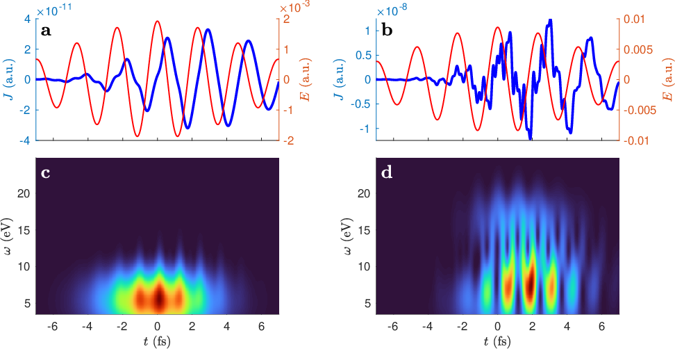
For low-order harmonics, it is commonly accepted that ionization gains importance as the damage threshold is approached RN243. Recently, the influence of the step-wise ionization on intraband currents has been discussed RN135; RN265; RN295. When the electrons begin to cover a significant range of the first Brillouin zone, the contribution of Bloch electrons to low-order harmonics is expected to change, as visualized in Fig. 1. An electron promoted to the conduction band () generates the current . With a rather short-range trajectory at low intensities, the current contains mainly fundamental frequencies. With increasing intensity, the electron motion becomes anharmonic and contains increasingly more third harmonic frequencies.
Here, this simple picture is extended to the motion of interband coherences, which give rise to the interband polarization. It is found that the nonlinear optical response from interband coherences (which are responsible for the reversible or transient or virtual population) changes abruptly as the crystal electrons explore the first Brillouin zone. This is observed by an interference structure in the third-order harmonic generation (THG). For short laser pulses, this happens already at intensities where the contribution of intraband currents due to ionization is not yet dominant. The mechanism is different from the influence of Bloch electron motion on intraband currents (which are seeded by the irreversible or real population), which has been observed before in HHG RN293; RN294. The observed effect is in the realm of perturbative optics, because the iterative series RN249 converges and reproduces the interference structure. The regime of intensities might be called almost-strong-field regime, because the intensities are smaller than in strong-field laser physics, yet the nonlinear response differs substantially from conventional nonlinear optics. Conventional nonlinear optics is understood here to indicate that the excursion of band electrons is negligible. Strong-field laser physics, on the other hand, is understood here to indicate that the response cannot be treated perturbatively, which implies a Keldysh parameter . The almost-strong-field regime, where the electron trajectories cover a significant range of the first Brillouin zone but the contribution of intraband currents is still negligible, is commonly reached in lenses and windows of high-power optical instruments, in contrast to the strong-field regime, where optical elements deteriorate quickly.

To uncover the expected interference, an intensity scan is required that extends from the regime of conventional nonlinear optics into the regime of Bloch electron motion. This introduces significant complications for the experiment, as the yield of harmonic light would cover a very wide range. To overcome this problem, non-collinear spectroscopy is used here, sketched in Fig. 2. Two visible-infrared (Vis-IR) pulses A and B are focused into 100-m-thick crystals with polarization perpendicular to the plane of incidence. A and B are overlapped spatially and temporally with a precision of m and fs, forming a laser induced grating RN18. Deep ultraviolet (DUV) light is produced by THG in the crystals. The DUV light that is emitted collinearly to A, which is kept at a constant intensity = 7 TW/cm2, is detected with a spectrometer. The intensity of B is varied in the range = [0, 8] TW/cm2, which varies the peak intensity in the grating. This facilitates intensity scans over a high dynamic range with little variation in spectrometer count rates.

The fundamental Vis-IR pulses are strongly modified by nonlinear pulse propagation, which obscures the observation of THG mechanisms. Fortunately, THG from the beginning of the crystals strongly contributes to the fringed DUV spectrum (Fig. 2 b). As previous studies RN192; RN194 revealed, the spectral fringes are produced by two DUV pulses that are well separated in time after the crystal. The leading pulse (labeled U) is in time with the Vis-IR pulse, whereas the trailing pulse (labeled V) propagates at the DUV group velocity RN192; RN194; RN263. V is beneficial for the interpretation of the data, because it is generated within the first few micrometers and maintains its spectrum in the subsequent linear propagation. The contribution of U complicates the interpretation of the data, because it is generated after nonlinear pulse propagation modified the fundamental pulses. Due to scattering of the Vis-IR light in the DUV spectrometer, the spectra contain also a significant background in addition to the fringed spectra . To remove the background and to enhance the sensitivity to V, the raw spectra are inverse Fourier transformed, the side peak (alternating component) is cut-out and shifted to zero, and thereafter Fourier transformed. This yields , where represents the shift to zero which corresponds to the delay between U and V after the medium. The parameters used are 87 fs for SiO2, 111 fs for Al2O3, 190 fs for MgO.
The intensity scan reveals an interference structure in the region = [10, 20] TW/cm2 for SiO2, see Fig. 2 c. As this is the regime where the crystal electrons explore the first Brillouin zone (Fig. 1), this is a first indication for THG from Bloch electrons that competes with conventional THG. Corresponding experiments in Al2O3 and MgO yield similar interferences (Extended Data Fig. 6), but fine details indicate that the band structure has an influence.
To get further insights, numerical calculations are performed using semiconductor Bloch equations (SBEs) RN218. With restriction to the spatial dimension of the electric field vector and omitting the Coulomb interaction, the SBEs read RN249; RN222
| (1) |
The diagonal elements of the density matrix are the populations of the electronic bands, the off-diagonal elements are the coherences between the states with transition energies . The electric field induces dynamics by coupling the electronic bands via the dipole matrix elements and by moving the electrons and holes within the bands, which is realized by the coordinate transform , where is the vector potential defined by . The relaxation terms are implemented as phenomenological damping terms (see Methods). The polarization and the current are calculated by
| (2) | ||||
| (3) |
where is the spacing in the -grid.
In most recent studies, the band structures are calculated by ab initio methods like density functional theory (DFT). Here, a different approach is taken. For a quantitative comparison of optical fields originating from macroscopic pulse propagation, it is essential that both the linear response (including the group velocity dispersion) and the nonlinear response (including the optical Kerr effect (OKE)) match the experiment. The linear response of DFT is known to deviate because of missing background contributions RN257; if the OKE is correctly reproduced is typically not tested. Here, numerical refractive index data is used to incorporate the linear polarization in the pulse propagation. The nonlinear polarization is used as a source term in the pulse propagation, which is calculated from equ. 2 in Fourier space by
| (4) |
where is the linear susceptibility of equ. 1 (see Methods). The dipole matrix elements of three-bands are then adjusted to match experimental data of the OKE. This supports pulse propagation using the unidirectional pulse propagation equation (UPPE) at feasible computation times, yet captures the interband and intraband dynamics consistently RN249.
The macroscopic UPPE calculations (see Methods), using the experimentally determined pulse shapes, confirm the assumption of two separate DUV pulses, see Fig. 3. The calculated spectra are processed like the experimental spectra. The Fourier-filtered spectrum , although somewhat masked by propagation effects, still resembles the THG at the beginning of the crystal (Fig. 3(d)). The reason is that V originates within the first few micrometers in the crystal and maintains its spectrum in the subsequent linear propagation. The intensity scan exhibits an interference structure that is similar to the experimental data. In order to investigate the influence of the band shape, calculations are performed where the band shape contains higher frequencies (Extended Data Fig. 7). As expected, the band shape influences the interference structure, which might be exploited to extract information about band shapes from the data. However, the calculations limited to three bands are unlikely to reproduce the interference structure in fine detail.

The interference structure also address a debated inconsistency in the field of HHG from solids. Numerical calculations by several groups agree that noisy spectra of HHG are predicted, in contrast to the clean harmonics measured experimentally. The most prominent solution of this discrepancy is to assume ultrafast coherence loss realized by dephasing times below fs, which helps the calculations produce clean harmonics RN241; RN224; RN242; RN221; RN239. The interference structure vanishes for such short dephasing times (Extended Data Fig. 11), which does not support the assumption of dephasing times below 10 fs.
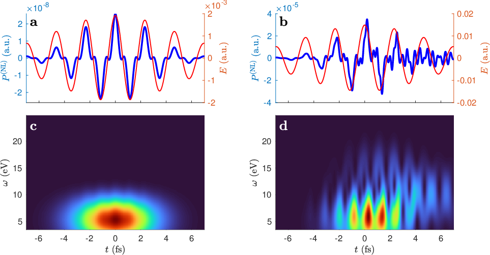
To clarify whether the interference structure is caused by a change of the mechanism of THG rather than propagation effects, the nonlinear response generated by 8-fs Gaussian pulses is investigated, see Fig. 4. exhibits an interference structure in the range [8, 20] TW/cm2, similar to the UPPE calculations and the experiment. The shape is influenced by the band shape (see Extended Data Figs. 8, 9, 10), but the general appearance is universal. Also shows an interference structure, but at lower intensities [2, 8] TW/cm2. This is an indication that the interference structure observed experimentally is not due to . This is affirmed by running the UPPE calculation with , which yields an indistinguishable result from the complete calculation displayed in Fig. 3 c. This seems to contradict recent wave-mixing experiments at similar intensities RN135; RN265, but a crucial point may be that the SBE calculations reproduce the reversible population of the conduction band RN134; RN182; RN249 rather than assuming a step-wise ionization.

The Keldysh parameter , where is the optical frequency, is commonly used to distinguish multiphoton () and strong-field () interactions RN226. While the former can be treated by the power series expansion of perturbative nonlinear optics, this series diverges for the latter. The transition region has attracted much attention for gases, where it is sometimes referred to as the regime of nonadiabatic tunneling RN254, but has not yet received much attention for solids. The intensity range of the interference structure ( at 8 TW/cm2 and at 18 TW/cm2) is below the regime of strong-field laser physics in the original sense. Strong-field laser physics in the original sense is understood here to mean that the power series expansion does not converge. To test the convergence, the SBEs are solved iteratively (see Methods and RN249). It has been shown before that the convergence criterion of the iteration is fulfilled for RN249. The pseudo color spectra produced with 100 iterations are distinguishable from those of the time-domain integration displayed in see Fig. 4 a. Only the line plot of Fig. 4 d reveals deviations starting at 18 TW/cm2 where .
To finally reveal the mechanism that causes the modification of the non-linear response in the almost-strong-field regime, a simplified calculation is performed neglecting the motion of the Bloch electrons. This is achieved by omitting the coordinate transform in (1). With the Bloch electron motion turned off, the interference structure in disappears. For lower intensities, displayed in the inset of Fig. 4 d, the calculations with and without Bloch electron motion agree perfectly. Thus, Bloch electron motion can be neglected at moderate intensities. Moreover, the instantaneous response , which is a common simplification for the OKE in transparent solids, is a very good approximation for these intensities. In the almost-strong-field regime, the THG intensity deviates from the instantaneous response model for both calculations with and without Bloch electron motion but only the full calculation generates the interference structures. At 5 TW/cm2, where exhibits interference, the electrons transverse up to 45% of the first Brillouin zone. However, this is not observed in the experiment because the influence of is still negligible at these low intensities. At 14 TW/cm2, where exhibits interference, the electrons transverse up to 75% of the first Brillouin zone. The origin of the nonlinear polarization in -space is traced by omitting the -summation in (2) resulting . In the almost-strong-field regime, the origin is shifted through the entire Brillouin zone (Fig. 4 d). This underpins the interpretation of Bloch motion that affects the interband polarization. At low intensities, only the local band curvature is decisive which is highest at . When the electrons start to explore the Brillouin zone, the band curvature throughout the trajectory must be considered both for the interband and for the intraband contribution of the nonlinear response.
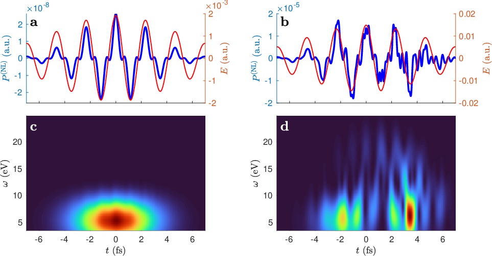
The spectrograms (Fig. 5 and Extended Data Fig. 12) show that while THG is temporally delocalized at low intensity, THG and also higher frequency generation are localized within the optical cycle at higher intensities. Some features are reminiscent of the three-step model for HHG RN258. In particular, there are branches with positive chirp, as typically associated with short electron trajectories, followed by branches with negative chirp, as typically associated with long trajectories. However, the three-step model would predict only photons with energies of band transitions RN241; RN261, which are limited to [10.3, 13.3] eV for the band structure used here. Furthermore, the highest photon energies are found at the peaks of the generating field, but the three-step model predicts them near the zero crossings. It is remarkable that the instantaneous response model fits very well for low intensity, but at higher intensity both the and exhibit dents at the field crests. These dents are clearly visible by comparing with the simplified calculation that neglects the motion of the Bloch electrons (Extended Data Fig. 13). These dents are reminiscent of the current generated by a single Bloch electron in Fig. 1. This strengthens the interpretation that Bloch electron motion can be regarded as a mechanism of harmonic generation not only for real electrons, which are the origin of and which was considered from the beginning as a possible mechanism for HHG, but also for virtual electrons (coherences), which are the origin of . In contrast to the original strong-field regime (), where optical components are very easily damaged, the almost-strong-field regime is often reached in high-power lasers and other optical instruments. The results of this work, especially numerical pulse propagation at feasible computation times, will be useful for the design of such instruments.
References
- (1) Haug, H., Koch, S.W.: Quantum Theory of the Optical and Electronic Properties of Semiconductors, 5th edn. World Scientific, ??? (2009)
- (2) Feldmann, J., Leo, K., Shah, J., Miller, D.A.B., Cunningham, J.E., Meier, T., Vonplessen, G., Schulze, A., Thomas, P., Schmittrink, S.: Optical investigation of bloch oscillations in a semiconductor superlattice. Physical Review B 46(11), 7252–7255 (1992)
- (3) Leo, K., Bolivar, P.H., Bruggemann, F., Schwedler, R., Kohler, K.: Observation of bloch oscillations in a semiconductor superlattice. Solid State Communications 84(10), 943–946 (1992)
- (4) Waschke, C., Roskos, H.G., Schwedler, R., Leo, K., Kurz, H., Kohler, K.: Coherent submillimeter-wave emission from bloch oscillations in a semiconductor superlattice. Physical Review Letters 70(21), 3319–3322 (1993)
- (5) Faisal, F.H.M., Kaminski, J.Z.: Floquet-bloch theory of high-harmonic generation in periodic structures. Physical Review A 56(1), 748–762 (1997)
- (6) Ghimire, S., DiChiara, A.D., Sistrunk, E., Agostini, P., DiMauro, L.F., Reis, D.A.: Observation of high-order harmonic generation in a bulk crystal. Nature Physics 7(2), 138–141 (2011)
- (7) Vampa, G., McDonald, C.R., Orlando, G., Klug, D.D., Corkum, P.B., Brabec, T.: Theoretical analysis of high-harmonic generation in solids. Phys Rev Lett 113(7), 073901 (2014)
- (8) Ndabashimiye, G., Ghimire, S., Wu, M.X., Browne, D.A., Schafer, K.J., Gaarde, M.B., Reis, D.A.: Solid-state harmonics beyond the atomic limit. Nature 534(7608), 520 (2016)
- (9) Luu, T.T., Garg, M., Kruchinin, S.Y., Moulet, A., Hassan, M.T., Goulielmakis, E.: Extreme ultraviolet high-harmonic spectroscopy of solids. Nature 521(7553), 498–502 (2015)
- (10) Schubert, O., Hohenleutner, M., Langer, F., Urbanek, B., Lange, C., Huttner, U., Golde, D., Meier, T., Kira, M., Koch, S.W., Huber, R.: Sub-cycle control of terahertz high-harmonic generation by dynamical bloch oscillations. Nature Photonics 8(2), 119–123 (2014)
- (11) Uzan-Narovlansky, A.J., Jimenez-Galan, A., Orenstein, G., Silva, R.E.F., Arusi-Parpar, T., Shames, S., Bruner, B.D., Yan, B.H., Smirnova, O., Ivanov, M., Dudovich, N.: Observation of light-driven band structure via multiband high-harmonic spectroscopy. Nature Photonics 16(6), 428 (2022)
- (12) Hohenleutner, M., Langer, F., Schubert, O., Knorr, M., Huttner, U., Koch, S.W., Kira, M., Huber, R.: Real-time observation of interfering crystal electrons in high-harmonic generation. Nature 523(7562), 572–5 (2015)
- (13) Kruchinin, S.Y., Krausz, F., Yakovlev, V.S.: Colloquium: Strong-field phenomena in periodic systems. Reviews of Modern Physics 90(2), 021002 (2018)
- (14) Floss, I., Lemell, C., Wachter, G., Smejkal, V., Sato, S.A., Tong, X.M., Yabana, K., Burgdorfer, J.: Ab initio multiscale simulation of high-order harmonic generation in solids. Physical Review A 97(1), 011401 (2018)
- (15) McDonald, C.R., Ben Taher, A., Brabec, T.: Strong optical field ionisation of solids. Journal of Optics 19(11), 114005 (2017)
- (16) Couairon, A., Sudrie, L., Franco, M., Prade, B., Mysyrowicz, A.: Filamentation and damage in fused silica induced by tightly focused femtosecond laser pulses. Physical Review B 71(12), 125435 (2005)
- (17) Mitrofanov, A.V., Verhoef, A.J., Serebryannikov, E.E., Lumeau, J., Glebov, L., Zheltikov, A.M., Baltuska, A.: Optical detection of attosecond ionization induced by a few-cycle laser field in a transparent dielectric material. Phys Rev Lett 106(14), 147401 (2011)
- (18) Jurgens, P., Liewehr, B., Kruse, B., Peltz, C., Engel, D., Husakou, A., Witting, T., Ivanov, M., Vrakking, M.J.J., Fennel, T., Mermillod-Blondin, A.: Origin of strong-field-induced low-order harmonic generation in amorphous quartz. Nature Physics 16(10), 1035 (2020)
- (19) Jurgens, P., Liewehr, B., Kruse, B., Peltz, C., Witting, T., Husakou, A., Rouzee, A., Ivanov, M., Fennel, T., Vrakking, M.J.J., Mermillod-Blondin, A.: Characterization of laser-induced ionization dynamics in solid dielectrics. Acs Photonics 9(1), 233–240 (2022)
- (20) Pfeiffer, A.N.: Iteration of semiconductor bloch equations for ultrashort laser pulse propagation. Journal of Physics B-Atomic Molecular and Optical Physics 53(16) (2020)
- (21) Pati, A.P., Reislohner, J., Leithold, C.G., Pfeiffer, A.N.: Effects of the groove-envelope phase in self-diffraction. Journal of Modern Optics 64(10-11), 1112–1118 (2017)
- (22) Reislöhner, J., Leithold, C., Pfeiffer, A.N.: Characterization of weak deep uv pulses using cross-phase modulation scans. Opt. Lett. 44(7), 1809–1812 (2019)
- (23) Reislöhner, J., Leithold, C., Pfeiffer, A.N.: Harmonic concatenation of 1.5 fs pulses in the deep ultraviolet. ACS Photonics 6(6), 1351–1355 (2019)
- (24) Babushkin, I.V., Noack, F., Herrmann, J.: Generation of sub-5 fs pulses in vacuum ultraviolet using four-wave frequency mixing in hollow waveguides. Optics Letters 33(9), 938–940 (2008)
- (25) Li, J.B., Zhang, X., Fu, S.L., Feng, Y.K., Hu, B.T., Du, H.C.: Phase invariance of the semiconductor bloch equations. Physical Review A 100(4), 043404 (2019)
- (26) Kilen, I., Kolesik, M., Hader, J., Moloney, J.V., Huttner, U., Hagen, M.K., Koch, S.W.: Propagation induced dephasing in semiconductor high-harmonic generation. Physical Review Letters 125(8) (2020)
- (27) Schultze, M., Bothschafter, E.M., Sommer, A., Holzner, S., Schweinberger, W., Fiess, M., Hofstetter, M., Kienberger, R., Apalkov, V., Yakovlev, V.S., Stockman, M.I., Krausz, F.: Controlling dielectrics with the electric field of light. Nature 493(7430), 75–8 (2013)
- (28) Sommer, A., Bothschafter, E.M., Sato, S.A., Jakubeit, C., Latka, T., Razskazovskaya, O., Fattahi, H., Jobst, M., Schweinberger, W., Shirvanyan, V., Yakovlev, V.S., Kienberger, R., Yabana, K., Karpowicz, N., Schultze, M., Krausz, F.: Attosecond nonlinear polarization and light-matter energy transfer in solids. Nature 534(7605), 86–90 (2016)
- (29) Keldysh, L.V.: Ionization in the field of a strong electromagnetic wave. JETP 20(5), 1307–1314 (1965)
- (30) Yudin, G.L., Ivanov, M.Y.: Nonadiabatic tunnel ionization: Looking inside a laser cycle. Physical Review A 64(1) (2001)
- (31) Lewenstein, M., Balcou, P., Ivanov, M.Y., Lhuillier, A., Corkum, P.B.: Theory of high-harmonic generation by low-frequency laser fields. Physical Review A 49(3), 2117–2132 (1994)
- (32) Sjakste, J., Tanimura, K., Barbarino, G., Perfetti, L., Vast, N.: Hot electron relaxation dynamics in semiconductors: assessing the strength of the electron-phonon coupling from the theoretical and experimental viewpoints. J Phys Condens Matter 30(35), 353001 (2018)
- (33) Schiffrin, A., Paasch-Colberg, T., Karpowicz, N., Apalkov, V., Gerster, D., Muhlbrandt, S., Korbman, M., Reichert, J., Schultze, M., Holzner, S., Barth, J.V., Kienberger, R., Ernstorfer, R., Yakovlev, V.S., Stockman, M.I., Krausz, F.: Optical-field-induced current in dielectrics. Nature 493(7430), 70–4 (2013)
Methods
Calculations based on SBEs
The consistent treatment of the OKE requires at least three bands RN249. Two valence bands (bands 1 and 3) and one conduction band (band 2) are considered here. In a realistic band structure, valence bands have typically a transition energy on the order of 1 eV, but resonance effects with the Vis-IR pulse do not prevail because many valence bands exist. To avoid resonance effects for only two valence bands, is assumed. However, only band 1 is coupled to the conduction band. Only the conduction band energy is considered to be -dependent with a tight-binding band shape:
| (5) |
with bandwidth eV and lattice constant nm. The bandgap is set to eV,
The dipole matrix elements are matched to the OKE at low intensities as described in Ref. RN249. The valence band transitions are implemented with . The valence to conduction band transitions are implemented as RN218
| (6) |
with . All other dipole matrix elements are set to zero.
Relaxation is implemented as phenomenological damping terms. For the diagonal elements, the lifetime and the collision time are considered.
| (7) |
The lifetime in conduction bands of dielectrics usually exceeds 100 fs, justifying the assumption . The terms proportional to causes a decay of the currents, while the total band population is preserved. The damping of the currents cannot be neglected, because Drude collision times are in the few-femtosecond range. This is in accordance with the qualitative picture of excited electrons that first undergo rapid momentum relaxation and thereafter energy relaxation on a longer timescale RN214. For the coherences,
| (8) |
where is the interband dephasing time. Here it is assumed that is identical for all coherences and independent on . The relation between the dephasing time and the Drude collision time is not known. Here, is assumed, following the phenomenological picture that if scattering occurs to an electron at position , its interband- and intraband coherences are likewise destroyed.
The numerical calculations are perfomed on a -grid with 27 points. The time-domain integration is performed using the 4th-order Runge–Kutta (RK4) method. For the calculations with pulse propagation (Figs. 3, 7 and 11), a -grid with 30001 points in the interval [-250, 250] fs is used. For the calculations without pulse propagation (all other Figures), a -grid with 70001 points in the interval [-500, 500] fs is used.
Iteration of SBEs
For dielectrics, the population transfer into the conduction band is only a small fraction of the valence band population when irreversible material changes are avoided. This justifies the assumptions ; ; , which effectively decouples the diagonal and off-diagonal elements of the SBEs. With this approximation the non-diagonal elements of (1) can be transformed to
| (9) |
with
| (10) |
Here, the time-dependent transition energy is separated into a static part and the dynamic part . The elements are the corrections due to the nonlinearity. A recursive method is used for their calculation: In the step of iteration, the elements in (9) are calculated using the elements of the step. Each step of iteration requires (inverse) Fourier transforms and time-domain multiplications. is assumed in step 0.
The iteration is equivalent to a power series expansion. Accordingly there is an upper limit for the electric field above which the iteration does not converge. In the limit of a monochromatic field with frequency , the convergence criterion is given by RN226.
The linear susceptibility follows from (9) by setting :
| (11) |
Pulse propagation
Macroscopic pulse propagation is calculated using the UPPE
| (12) |
where the hat symbol indicates the Fourier transform in the dimensions of time and transverse space. In addition to the propagation direction , one transverse dimension (the -dimension) is included to account for the noncollinear geometry with . Numerical tables are used for the refractive index , is the speed of light and is the group velocity of the Vis-IR pulse. The electric field is treated as scalar field, because all pulses are polarized perpendicular to the plane of incidence.
The UPPE is integrated numerically using the split-step method with an -grid with 81 points in the interval [-260, 260] m and a -grid with 401 points in the interval [0, 100] m.
Subsequent to the propagation inside the crystal, the light propagating collinearly to A with emission angle is calculated by
| (13) |
with .
Acknowledgement
This project was supported primarily by the Deutsche Forschungsgemeinschaft (DFG, German Research Foundation) via Priority Programme 1840 ”Quantum Dynamics in Tailored Intense Fields (QUTIF)” (project ID 281272215) and via project B1 in the Collaborative Research Centre 1375 ”Nonlinear optics down to atomic scales (NOA)” (project ID 398816777).
Author Contributions
JR conducted the experiment. ANP developed the theory. All authors contributed to the discussion and preparation of the manuscript.