A Spectral Analysis of Graph Neural Networks on Dense and Sparse Graphs

The canonical statistical model for graphs with communities is the stochastic block model (SBM).

Spectral methods for community detection are inspired by the spectral decomposition of the SBM. Consider for example the case where $K=2$, ${\mathbf{B}}=[p\ q;q\ p]$, $p\neq q$, and the communities are balanced, i.e., $N$ is even and both communities have size $N/2$. Relabeling ${\mathcal{V}}$ so that the first $N/2$ nodes belong to the first community and the remaining $N/2$ to the second, we see that the eigenvectors of ${\mathbb{E}}{\mathbf{A}}\equiv{\mathbf{P}}$, the expected adjacency, are given by

For a graph ${\mathbf{G}}$ sampled from this model, with sufficiently large $N$ and mild assumptions on $p,q$, we can thus expect the eigenvector ${\mathbf{v}}_{2}({\mathbf{A}})$ to provide a good estimate of its community structure, i.e., ${\mathbf{v}}_{k}({\mathbf{A}})\approx{\mathbf{v}}_{k}({\mathbb{E}}{\mathbf{A}}),k\in\{1,2\}$.

Real-world graphs ${\mathbf{G}}$ have more intricate sparsity patterns than the SBM, but it is reasonable to assume that if the graph ${\mathbf{G}}$ has two balanced communities, for some permutation of the nodes its adjacency matrix ${\mathbf{A}}$ can be approximately written as ${\mathbf{A}}={\mathbf{A}}_{\tiny\mbox{SBM}}+{\mathbf{E}}$, where ${\mathbf{A}}{\tiny\mbox{SBM}}$ is as in Def. 1 and ${\mathbf{E}}$ can be seen as a perturbation satisfying $\|{\mathbf{E}}\|_{2}<\|{\mathbf{A}}{\tiny\mbox{SBM}}\|_{2}$. As such, the first two eigenvectors of ${\mathbf{A}}$ still “embed” community information. More generally, in graphs ${\mathbf{G}}$ with $K>2$ balanced communities, the community information is “embedded” in the first $K$ eigenvectors. Based on this observation, the order-$K$ spectral embedding of a graph ${\mathbf{G}}$ is defined as

i.e., as the concatenation of the first $K$ eigenvectors of ${\mathbf{A}}$. Variants of SE tailored for sparse graphs propose replacing ${\mathbf{A}}$ with other graph operators, such as the normalized adjacency matrix $\tilde{{\mathbf{A}}}\coloneqq{\mathbf{D}}^{-0.5}{\mathbf{A}}{\mathbf{D}}^{-0.5}$ where ${\mathbf{D}}$ is the degree matrix [23], the non-backtracking operator [10], etc.

Note that $\phi_{\tiny\mbox{SE}}$ is nonparametric; it can be obtained directly from the graph without node label supervision. When we use spectral embeddings in (2), the only parameters that are learned are those of the classifier $c$. E.g., choosing a linear classifier yields a simple parameterization of $f$ as $f({\mathbf{A}})=c\circ\phi_{\tiny\mbox{SE}}({\mathbf{A}})=\mbox{{softmax}}({\mathbf{V}}_{K}{\mathbf{C}})$ where ${\mathbf{C}}\in{\mathbb{R}}^{K\times K}$ is learned. More generally, it is possible to use embeddings $\phi_{\tiny\mbox{SE}}({\mathbf{A}})={\mathbf{V}}_{\tilde{K}}$ with $\tilde{K}>K$, i.e., with a larger number of eigenvectors than that of communities, in which case ${\mathbf{C}}\in{\mathbb{R}}^{\tilde{K}\times K}$.

An important observation to make is that $\phi_{\tiny\mbox{SE}}$ (and so $f$) do not need to depend on ${\mathbf{X}}$, but if such node features are available, they can be incorporated into the spectral embedding in different ways, e.g., [24, 25, 26, 27, 28]. We consider an approach similar to [26], by first embedding the node feature covariance and concatenating it with the spectral embedding. More precisely, let ${\mathbf{V}}^{\prime}_{\kappa}$ be the first $\kappa$ eigenvectors of the covariance matrix ${\mathbf{X}}{\mathbf{X}}^{\top}$, then the feature-aware spectral embedding is defined as

Given a graph ${\mathbf{G}}$ with adjacency matrix ${\mathbf{A}}\in{\mathbb{R}}^{N\times N}$ and a graph signal ${\mathbf{x}}\in{\mathbb{R}}^{N}$, a graph convolution (or filter) is given by [29]

where $h_{0},\ldots,h_{K-1}$ are the filter coefficients or taps. More generally, if ${\mathbf{X}}\in{\mathbb{R}}^{N\times D}$ and ${\mathbf{U}}\in{\mathbb{R}}^{N\times G}$ have $D$ and $G$ features respectively, we write

where the filter parameters are now collected in the matrices ${\mathbf{H}}_{0},\ldots,$ ${\mathbf{H}}_{K-1}\in{\mathbb{R}}^{D\times G}$.

Graph neural networks (GNNs) are deep convolutional architectures where each layer composes a graph convolution (7) and a pointwise nonlinearity $[\sigma({\mathbf{U}})]_{ij}=\sigma([{\mathbf{U}}]_{ij})$, e.g., the ReLU or the sigmoid. The $\ell$th layer of a GNN can thus be written as

where ${\mathbf{X}}_{\ell-1}\in{\mathbb{R}}^{N\times F_{\ell-1}}$ and ${\mathbf{X}}_{\ell}\in{\mathbb{R}}^{N\times F_{\ell}}$ are the input and output to this layer with $F_{\ell-1}$ and $F_{\ell}$ features each. If the GNN has $L$ layers, its input and output are ${\mathbf{X}}_{0}={\mathbf{X}}\in{\mathbb{R}}^{N\times F_{0}}$ and ${\mathbf{X}}_{L}\in{\mathbb{R}}^{N\times F_{L}}$.

The GNN in (8) may be used to parametrize $\phi$ in (2), in which case we define the GNN embedding

Note that, unlike the spectral embedding (4), (9) is parametric on $\{{\mathbf{H}}_{\ell k}\}_{\ell,k}$ and always needs an input signal ${\mathbf{X}}$ (if an input signal is not available, ${\mathbf{X}}$ may be a random signal, for example). A typical parametrization of $f$ for GNN embeddings is $f({\mathbf{A}},{\mathbf{X}})=c\circ\phi_{\tiny\mbox{GNN}}({\mathbf{A}},{\mathbf{X}})=\mbox{{softmax}}({\mathbf{X}}_{L}{\mathbf{C}})$ where ${\mathbf{C}}\in{\mathbb{R}}^{F_{L}\times K}$ is a linear classifier over $F_{L}$ node features. This is equivalent to a $L+1$-layer GNN with $K=1$ and softmax nonlinearity in the last layer.

Def. 2 introduces a random graph model allowing to model graphs with varying levels of sparsity according to a sparsity parameter $\gamma$.

This model allows sampling both dense and sparse graphs because, since ${\mathbf{W}}$ has vanishing tails (or can be mapped to a kernel that does by some measure-preserving transformation), for a fixed $N$ the graph is sparser for larger $\gamma$.

The kernel ${\mathbf{W}}$ defines a self-adjoint Hilbert Schmidt operator. Hence, it has a real spectrum given by

where the eigenvalues $\lambda_{i}$ are countable and the eigenfunctions $\varphi_{i}$ form an orthonormal basis of $L^{2}$. By convention, the eigenvalues are ordered as $|\lambda_{1}|\geq|\lambda_{2}|\geq\ldots$. Moreover, $|\lambda_{i}|\leq\infty$ for all $i$, and $\lambda_{i}\to 0$ as $i\to\infty$ with zero being the only accumulation point.

We further introduce the notion of a kernel induced by a graph, which will be useful in future derivations. For $N\geq 2$, the kernel induced by the graph ${\mathbf{G}}_{N}$ with adjacency ${\mathbf{A}}_{N}$ and sparsity parameter $\gamma$ is defined as

where $I_{i}=[u_{i},u_{i+1})$ for $1\leq i\leq N-2$, $I_{N-1}=[u_{N-1},u_{N}]$, and $u_{i}$ is as in Def. 2.

To discuss community detection on graphs sampled from a DSGM (Def. 2), we assume that the kernel ${\mathbf{W}}$ exhibits community structure. For simplicity, we focus on $2$ communities but the discussions can be easily extended to $K$ communities. Inspired by the degree-corrected SBM [30, 31], in Def. 3 we introduce the degree-corrected stochastic block kernel (SBK) as the canonical kernel for DSGMs with $2$ balanced communities. This model is suitable to model sparse graphs and well-studied in the spectral embedding literature [31, 23]. To ensure that models based on these kernels are valid DSGMs, we restrict attention to finite-energy degree functions $\theta$.

It is not difficult to see that the first $2$ eigenfunctions of ${\mathbf{W}}$ in Def. 3 reveal the community structure ¹¹ 1 $\varphi_{1}(u)=\theta(u)/C,\varphi_{2}(u)=\big(-\theta(u){\mathbb{I}}(u<0)+\theta(u){\mathbb{I}}(u\geq 0)\big)/C,\\ \text{ where }C\coloneqq\int\theta(u)du$.. For graphs ${\mathbf{G}}_{N}$ sampled as in Def. 2 from the DSGM with degree-corrected kernel as in Def. 3, the true community assignment is given by $[{\mathbf{Y}}]_{i\cdot}=Y(u_{i})$ for $1\leq i\leq N$. As such, the quality of the estimate of the community assignment given by the first $2$ (or, more generally, the first $K$) eigenvectors of ${\mathbf{G}}_{N}$ will depend on both (i) how close the eigenvalues $\lambda_{k}({\mathbf{G}}_{N})$ are to the kernel eigenvalues $\lambda_{k}({\mathbf{W}})$ (as this can affect their ordering) and (ii) how close the eigenvectors ${\mathbf{v}}_{k}$ are to the eigenfunctions $\varphi_{k}$. These differences are upper bounded by Thm. 1.

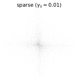
This theorem shows that the differences between the eigenvalues and eigenvectors of the graph and the underlying random graph model are upper bounded by terms that increase with $\gamma$. Consider a dense graph ${\mathbf{G}}_{N}^{d}$ and a sparse graph ${\mathbf{G}}_{N}^{s}$ sampled from DSGMs with same kernel ${\mathbf{W}}$ but different sparsity parameters $\gamma_{d}\ll\gamma_{s}$. If $N$ and $c$ are large enough for the term depending on $4A_{w}c\gamma$ to dominate the bound in the dense case, the bound on the difference between eigenvalues and eigenvectors in the sparse case is much larger than in the dense case. In the context of community detection, this can be interpreted to mean that, since $\varphi_{k}({\mathbf{W}}_{N}^{d})$ is close to $\varphi_{k}({\mathbf{W}})$ for dense graphs, some linear combination of the eigenvectors ${\mathbf{v}}_{k}({\mathbf{G}}_{N}^{d})$ provides a good estimate of the true community assignment ${\mathbf{Y}}$. This is not true for the eigenvectors ${\mathbf{v}}_{k}({\mathbf{G}}_{N}^{s})$ of the sparse graph, since $\varphi_{k}({\mathbf{W}}_{N}^{s})$ is further away from $\varphi_{k}({\mathbf{W}})$. Another way to think about this is that on dense graphs most of the “community information” is on the first $K$ eigenvectors. On sparse graphs, it is more spread throughout the spectrum. This implies that while spectral embeddings may be effective for community detection on dense graphs, they are less likely to be effective in sparse graphs. We further demonstrate this empirically in Sec. 4.

In sparse graphs, GNN embeddings are a better option than spectral embeddings because, provided that the input signal ${\mathbf{X}}_{{\mathcal{T}}}$ in (1) is not orthogonal to any of the graph’s eigenvectors, GNNs “have access” to the entire spectrum. Moreover, if the true community assignment signal is ${\mathbf{Y}}$, a GNN can always represent ${\mathbf{Y}}$ with $K\leq N$ in (8). These claims are formally stated for the simple graph convolution (6) in Thm. 2. They can be readily extended to multi-feature graph convolutions (7) and GNNs (8) where the nonlinearity $\sigma$ preserves the sign (e.g., the hyperbolic tangent).

Note that the assumptions of Thm. 2 are not too restrictive; most real-world graphs are full rank, and even a random signal ${\mathbf{x}}\in{\mathbb{R}}^{N}$—which may be used as the input in (9) when ${\mathbf{x}}$ is not given—satisfies $[{\mathbf{V}}^{\top}{\mathbf{x}}]_{i}\neq 0$ with high probability. It is also worth pointing out that while $K\leq N$ is necessary to exactly represent ${\mathbf{y}}$, in practice small $K$ is often enough to obtain good approximations of the true community assignment as illustrated in Sec. 4. This is another reason why in practical, large graph settings, GNN embeddings are advantageous w.r.t. spectral embeddings: a small number of matrix-vector multiplications requires less computations than calculating a number of eigenvectors at least as large as the number of communities.

The proof of Theorem 1 relies on slight variations of the Courant-Fisher and Davis-Kahan theorems, stated here as Propositions 1 and 2.

We thus only need to bound $\|{\mathbf{W}}-{\mathbf{W}}_{N}\|$. To do so, define $\overline{{\mathbf{W}}}_{N}$ as

where $I_{i}=[u_{i},u_{i+1})$ for $1\leq i\leq N-2$, $I_{N-1}=[u_{N-1},u_{N}]$, and $u_{i}$ is as in (2). Using the triangle inequality, we can write

The norm difference between $\overline{{\mathbf{W}}}_{N}$ and ${\mathbf{W}}_{N}$ is bounded as $N^{-1}\beta(\chi,N)$ by [7, Proposition 4] and by the fact that $\|{\mathbf{W}}_{N}\|_{L_{2}}=N^{-1}\|{\mathbf{A}}_{N}\|_{2}$ (see [32, Lemma 2]). Let us now derive a bound for $\|{\mathbf{W}}-\overline{{\mathbf{W}}}_{N}\|$.

By definition of the $L^{2}$ norm,

The rightmost term is bounded by $\epsilon(c)$, as $\overline{{\mathbf{W}}}_{N}$ is zero outside of $[-c,c]$. Since ${\mathbf{W}}$ is $A_{w}$-Lispchitz in the $[-c,c]$ interval, we can write

for $u_{i}\leq u\leq u_{i+1}$, $u_{j}\leq v\leq u_{j+1}$, where the $u_{i}$, $u_{j}$ are as in Definition 2 for all $1\leq i,j\leq N$. Therefore, the leftmost term in (15) can be upper bounded as $\sqrt{2c\times 2c\times({2A_{w}}{\gamma})^{2}}=4A_{w}\gamma c$, which completes the proof.

Theorem 2.1 is a direct consequence of the fact that the graph convolution is pointwise in the spectral domain. To see this, substitute ${\mathbf{A}}={\mathbf{V}}\bm{\Lambda}{\mathbf{V}}^{\top}$ in (6) and left-multiply both sides by ${\mathbf{V}}^{\top}$. We get

Hence, Theorem 2.1 holds for any $h_{k}\neq 0$.

Data. The Chameleon webpage network has $2277$ nodes with average node degree $13.8$, where nodes represent webpages and edges are hyperlinks between them. The node features are $2325$-dimensional bag-of-words vectors of the webpages, and node labels are $5$ webpage categories. We use the same data splits (48/32/20 for train/validation/test) from [36] released in Pytorch Geometric [37].

References

- [1] Lovro Vrćek, Xavier Bresson, Thomas Laurent, Martin Schmitz, and Mile Šikić, “Reconstruction of short genomic sequences with graph convolutional networks,” in 2023 46th MIPRO ICT and Electronics Convention (MIPRO). IEEE, 2023, pp. 403–409.
- [2] Sydney Dolan, Siddharth Nayak, and Hamsa Balakrishnan, “Satellite navigation and coordination with limited information sharing,” in Learning for Dynamics and Control Conference. PMLR, 2023, pp. 1058–1071.
- [3] Nicolas Keriven and Gabriel Peyré, “Universal invariant and equivariant graph neural networks,” Advances in Neural Information Processing Systems, vol. 32, 2019.
- [4] K. Xu, W. Hu, J. Leskovec, and S. Jegelka, “How powerful are graph neural networks?,” in 7th Int. Conf. Learning Representations, New Orleans, LA, 6-9 May 2019, pp. 1–17, Assoc. Comput. Linguistics.
- [5] Jan Böker, Ron Levie, Ningyuan Huang, Soledad Villar, and Christopher Morris, “Fine-grained expressivity of graph neural networks,” arXiv preprint arXiv:2306.03698, 2023.
- [6] F. Gama, J. Bruna, and A. Ribeiro, “Stability properties of graph neural networks,” IEEE Trans. Signal Process., vol. 68, pp. 5680–5695, 2020.
- [7] L. Ruiz, L. F. O. Chamon, and A. Ribeiro, “Transferability properties of graph neural networks,” arXiv:2112.04629 [eess.SP]. Submitted to IEEE TSP, 2021.
- [8] L. Ruiz, F. Gama, and A. Ribeiro, “Graph neural networks: Architectures, stability and transferability,” Proc. IEEE, vol. 109, no. 5, pp. 660–682, 2021.
- [9] A. Athreya, D. E. Fishkind, M. Tang, C. E. Priebe, Y. Park, J. T. Vogelstein, K. Levin, V. Lyzinski, and Y. Qin, “Statistical inference on random dot product graphs: a survey,” The Journal of Machine Learning Research, vol. 18, no. 1, pp. 8393–8484, 2017.
- [10] E. Abbe, “Community detection and stochastic block models: recent developments,” The Journal of Machine Learning Research, vol. 18, no. 1, pp. 6446–6531, 2017.
- [11] Aseem Baranwal, Kimon Fountoulakis, and Aukosh Jagannath, “Graph convolution for semi-supervised classification: Improved linear separability and out-of-distribution generalization,” arXiv preprint arXiv:2102.06966, 2021.
- [12] Aseem Baranwal, Kimon Fountoulakis, and Aukosh Jagannath, “Effects of graph convolutions in multi-layer networks,” arXiv preprint arXiv:2204.09297, 2022.
- [13] Xiyuan Wang and Muhan Zhang, “How powerful are spectral graph neural networks,” in International Conference on Machine Learning. PMLR, 2022, pp. 23341–23362.
- [14] Qian Huang, Horace He, Abhay Singh, Ser-Nam Lim, and Austin R Benson, “Combining label propagation and simple models out-performs graph neural networks,” arXiv preprint arXiv:2010.13993, 2020.
- [15] Jiong Zhu, Yujun Yan, Lingxiao Zhao, Mark Heimann, Leman Akoglu, and Danai Koutra, “Beyond homophily in graph neural networks: Current limitations and effective designs,” Advances in neural information processing systems, vol. 33, pp. 7793–7804, 2020.
- [16] Yao Ma, Xiaorui Liu, Neil Shah, and Jiliang Tang, “Is homophily a necessity for graph neural networks?,” arXiv preprint arXiv:2106.06134, 2021.
- [17] Zhixian Chen, Tengfei Ma, and Yang Wang, “When does a spectral graph neural network fail in node classification?,” arXiv preprint arXiv:2202.07902, 2022.
- [18] A. Ortega, P. Frossard, J. Kovačević, J. M. F. Moura, and P. Vandergheynst, “Graph signal processing: Overview, challenges, and applications,” Proc. IEEE, vol. 106, no. 5, pp. 808–828, 2018.
- [19] A. Sandryhaila and J. M. F. Moura, “Discrete signal processing on graphs,” IEEE Trans. Signal Process., vol. 61, pp. 1644–1656, Apr. 2013.
- [20] J. Xie, S. Kelley, and B. K. Szymanski, “Overlapping community detection in networks: The state-of-the-art and comparative study,” ACM Computing Surveys (csur), vol. 45, no. 4, pp. 1–35, 2013.
- [21] D. S. Choi, P. J. Wolfe, and E. M. Airoldi, “Stochastic blockmodels with a growing number of classes,” Biometrika, vol. 99, no. 2, pp. 273–284, 2012.
- [22] T. T. Cai, T. Liang, and A. Rakhlin, “Weighted message passing and minimum energy flow for heterogeneous stochastic block models with side information.,” J. Mach. Learn. Res., vol. 21, pp. 11–1, 2020.
- [23] J. Cape, M. Tang, and C. E. Priebe, “On spectral embedding performance and elucidating network structure in stochastic blockmodel graphs,” Network Science, vol. 7, no. 3, pp. 269–291, 2019.
- [24] J. Yang, J. McAuley, and J. Leskovec, “Community detection in networks with node attributes,” in 2013 IEEE 13th International Conference on Data Mining, 2013, pp. 1151–1156.
- [25] N. Binkiewicz, J. T. Vogelstein, and K. Rohe, “Covariate-assisted spectral clustering,” Biometrika, vol. 104, no. 2, pp. 361–377, 2017.
- [26] J. Arroyo, A. Athreya, J. Cape, G. Chen, C. E. Priebe, and J. T. Vogelstein, “Inference for multiple heterogeneous networks with a common invariant subspace,” Journal of Machine Learning Research, vol. 22, no. 142, 2021.
- [27] C. Mu, A. Mele, L. Hao, J. Cape, A. Athreya, and C. E. Priebe, “On spectral algorithms for community detection in stochastic blockmodel graphs with vertex covariates,” IEEE Transactions on Network Science and Engineering, 2022.
- [28] Angelo Mele, Lingxin Hao, Joshua Cape, and Carey E Priebe, “Spectral inference for large stochastic blockmodels with nodal covariates,” arXiv preprint arXiv:1908.06438, 2019.
- [29] J. Du, J. Shi, S. Kar, and J. M. F. Moura, “On graph convolution for graph CNNs,” in 2018 IEEE Data Sci. Workshop, Lausanne, Switzerland, 4-6 June 2018, pp. 239–243, IEEE.
- [30] B. Karrer and M. E. J. Newman, “Stochastic blockmodels and community structure in networks,” Physical Review E, vol. 83, no. 1, pp. 016107, 2011.
- [31] T. Qin and K. Rohe, “Regularized spectral clustering under the degree-corrected stochastic blockmodel,” Advances in Neural Information Processing Systems, vol. 26, 2013.
- [32] L. Ruiz, L. F. O. Chamon, and A. Ribeiro, “Graphon signal processing,” IEEE Trans. Signal Process., vol. 69, pp. 4961–4976, 2021.
- [33] B. Rozemberczki, C. Allen, and Rik Sarkar, “Multi-scale attributed node embedding,” Journal of Complex Networks, vol. 9, no. 2, pp. cnab014, 2021.
- [34] L. Ruiz, L. F. O. Chamon, and A. Ribeiro, “Graphon neural networks and the transferability of graph neural networks,” in 34th Neural Inform. Process. Syst., Vancouver, BC (Virtual), 6-12 Dec. 2020, NeurIPS Foundation.
- [35] A. Seelmann, “Notes on the sin 2 theorem,” Integral Equations and Operator Theory, vol. 79, no. 4, pp. 579–597, 2014.
- [36] H. Pei, B. Wei, K. C-C. Chang, Y. Lei, and B. Yang, “Geom-gcn: Geometric graph convolutional networks,” in International Conference on Learning Representations, 2020.
- [37] M. Fey and J. E. Lenssen, “Fast graph representation learning with PyTorch Geometric,” in ICLR Workshop on Representation Learning on Graphs and Manifolds, 2019.
5 Appendix
5.1 Proof of Theorem 1