跳到论文正文
W Papers独立论文阅读器 arXiv:2211.02756 论文正文 计算阅读时间 · 0%
引用这篇论文根据当前论文元数据生成,正式投稿前建议核对。


License: CC BY 4.0
arXiv:2211.02756v2 [quant-ph] 30 Mar 2023

Quantum weight enumerators and tensor networks

ChunJun Cao Thanks: C. Cao is at the Institute for Quantum Information and Matter, California Institute of Technology.    Brad Lackey Thanks: B. Lackey is at Microsoft Quantum, Microsoft Corporation.
Abstract

We examine the use of weight enumerators for analyzing tensor network constructions, and specifically the quantum lego framework recently introduced. We extend the notion of quantum weight enumerators to so-called tensor enumerators, and prove that the trace operation on tensor networks is compatible with a trace operation on tensor enumerators. This allows us to compute quantum weight enumerators of larger codes such as the ones constructed through tensor network methods more efficiently. We also provide a general framework for quantum MacWilliams identities that includes tensor enumerators as a special case.

Index Terms: 
Quantum codes, weight enumerators, tensor networks, MacWilliams identity

This work has been submitted to the IEEE for possible publication. Copyright may be transferred without notice, after which this version may no longer be accessible.

I Introduction

The weight enumerator of a classical code counts the number of codewords at each Hamming weight, typically presented as a polynomial in a single indeterminate zz where the coefficient of zwz^{w} is the number of codewords of Hamming weight ww. The distance of the code can be extracted as the smallest (nonzero) degree where the enumerator has a positive coefficient. The MacWilliams identity [1] famously relates the weight enumerator of a code with that of its dual code.

Shor and Laflamme introduced two quantum weight enumerators [2] related by an analogue of the MacWilliams identity. For stabilizer codes, the AA-enumerator counts the number of stabilizers at each Hamming weight (i.e. the number of non-identity Pauli operators) while the BB-enumerator counts the number of logical operators at each Hamming weight. The distance of a stabilizer code is then the smallest degree where the coefficient (up to appropriate normalization) of BB strictly exceeds that of AA. For completeness, we will recount this in Section III below. Note that in terms of error detection, the difference of BB and AA expresses the probability of an undetected error even when the underlying code is not a stabilizer code [3].

Other quantum enumerators have been introduced, such as the “shadow” enumerator of [4, 5] to create bounds on the length, dimension, and distance for which quantum codes can exist. In [6, 7], the authors introduce quantum enumerators for asymmetric errors that count the types of Pauli operators that appear in a stabilizer/logical operator.

In this work we introduce a quantum weight enumerator formalism for tensor network constructions of quantum codes and in particular those from the recent quantum lego formalism [8]11 1 See also a related approach [9].. We will also examine its detailed applications to quantum error correcting codes using tensor networks in a companion paper [10]. In particular, the enumerators of Shor and Laflamme (or Hu, et al.) are “scalar” enumerators in our theory. We introduce vector and tensor enumerators whose coefficients are scalar enumerators, and show that tracing these enumerators in a tensor network recovers the Shor and Laflamme enumerators. We prove an analogue of the MacWilliams identity for tensor enumerators (Theorem V.2).

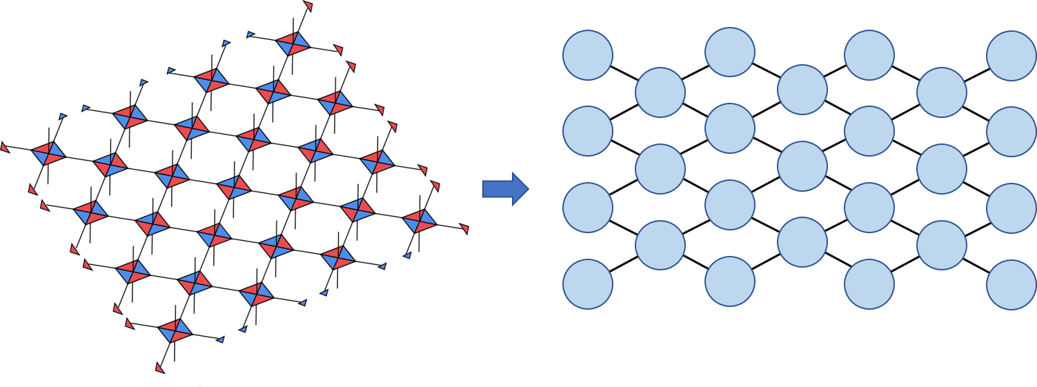
We also prove tensor enumerators are well-behaved under tensor product of the underlying networks: the tensor enumerator of a tensor product is the tensor product of the component enumerators (Proposition V.3). We also show that the trace of two legs in a tensor network extends to tensor enumerators, in that the enumerator of the trace can be computed by performing the trace of tensor enumerator along the corresponding legs (Theorem VII.1). In this way we can compute enumerators of large quantum codes constructed through tensor network methods.

II Definitions

A unitary basis on a Hilbert space ℌ\mathfrak{H} of dim(ℌ)=q\dim(\mathfrak{H})=q is a set of unitary operators ℰ\mathcal{E} containing II that form an orthonormal basis of L⁡(ℌ)L(\mathfrak{H}), in that Tr⁡(E​F†)=0\Tr(EF^{\dagger})=0 if E≠FE\not=F [11]. While quantum weight enumerators can be defined relative to a general unitary basis, to obtain important results such as a MacWilliams identity we require the basis have some additional structure. We focus on a class of “nice error bases” [12, 13], those with Abelian index group [14]. To avoid unnecessary repetition, we will simply refer to these as an “error basis” formally defined as follows.

Definition II.1.

An error basis on a Hilbert space is a unitary basis ℰ\mathcal{E} that additionally satisfies

E​F=ω⁡(E,F)​F​EEF=\omega(E,F)FE (II.1)

for all E,F∈ℰE,F\in\mathcal{E}, where ω⁡(E,F)∈ℂ\omega(E,F)\in\mathbb{C} satisfies ω​(E,F)r=1\omega(E,F)^{r}=1 for some fixed rr.

Perhaps the most important example of such a basis in the (generalized) Pauli group. This group is generated by operators X,ZX,Z, where

Z⁡|j⟩=ζj​|j⟩​ and ​X​|j⟩=|j+1​ (mod q)⟩,Z|{j}\rangle=\zeta^{j}|{j}\rangle\text{ and }X|{j}\rangle=|{j+1\text{ (mod $q$)}}\rangle,

where ζ=e2​π​i/q\zeta=e^{2\pi i/q}. That is, the eigenvalues of ZZ are the qq-th roots-of-unity, and on its eigenbasis XX acts as cyclic shift. Then X​Z=ζ−1​Z​XXZ=\zeta^{-1}ZX. The Pauli basis is

𝒫={XaZa′:a,a′∈{0,…,q−1}},\mathcal{P}=\{X^{a}Z^{a^{\prime}}\>:\>a,a^{\prime}\in\{0,\dots,q-1\}\},

and ω⁡(Xa​Za′,Xb​Zb′)=ζ(a′​b−a​b′)\omega(X^{a}Z^{a^{\prime}},X^{b}Z^{b^{\prime}})=\zeta^{(a^{\prime}b-ab^{\prime})}.

Given an error basis for ℌ\mathfrak{H}, we obtain one for ℌ⊗n\mathfrak{H}^{\otimes n} via

ℰn={E1⊗⋯⊗En: each Ej∈ℰ}.\mathcal{E}^{n}=\{E_{1}\otimes\cdots\otimes E_{n}\>:\>\text{ each }E_{j}\in\mathcal{E}\}.

Equation (II.1) holds where we define ω\omega on ℰn×ℰn\mathcal{E}^{n}\times\mathcal{E}^{n} to be the product of the ω\omega on each component. In particular, for the Pauli group ω⁡(X𝐚​Z𝐚′,X𝐛​Z𝐛′)=ζ𝐚′⋅𝐛−𝐚⋅𝐛′\omega(X^{\mathbf{a}}Z^{\mathbf{a}^{\prime}},X^{\mathbf{b}}Z^{\mathbf{b}^{\prime}})=\zeta^{\mathbf{a}^{\prime}\cdot\mathbf{b}-\mathbf{a}\cdot\mathbf{b}^{\prime}}, where X𝐚=Xa1⊗⋯⊗XanX^{\mathbf{a}}=X^{a_{1}}\otimes\cdots\otimes X^{a_{n}} and similarly for the the other terms.

The weight of such an operator is the number of non-identity tensor factors it contains, wt(E1⊗⋯⊗En)=|{r:Er≠I}|\mathrm{wt}(E_{1}\otimes\cdots\otimes E_{n})=|\{r\>:\>E_{r}\not=I\}|. Write ℰn​[d]\mathcal{E}^{n}[d] for the set of weight dd operators in the error basis.

Given an error basis ℰ\mathcal{E} on a Hilbert space ℋ\mathcal{H}, Shor and Laflamme [2] define two quantum weight enumerators22 2 We opt for the normalization in [4] as opposed to that in [2], and take a different convention in conjugate linearity. for a pair of Hermitian operators M1M_{1} and M2M_{2},

Ad​(M1,M2)\displaystyle A_{d}(M_{1},M_{2}) =∑E∈ℰn​[d]Tr⁡(E†​M1)​Tr⁡(E​M2),\displaystyle=\sum_{E\in\mathcal{E}^{n}[d]}\Tr(E^{\dagger}M_{1})\Tr(EM_{2}), (II.2)
Bd​(M1,M2)\displaystyle B_{d}(M_{1},M_{2}) =∑E∈ℰn​[d]Tr⁡(E†​M1​E​M2).\displaystyle=\sum_{E\in\mathcal{E}^{n}[d]}\Tr(E^{\dagger}M_{1}EM_{2}). (II.3)

We will often drop M1,M2M_{1},M_{2} from this notation when they are understood. While it is not obvious from this definition, both these values are invariant under local unitary transformations. That is, if U=U1⊗⋯⊗UnU=U_{1}\otimes\cdots\otimes U_{n} is any local unitary then

Ad​(U​M1​U†,U​M2​U†)=Ad​(M1,M2)A_{d}(UM_{1}U^{\dagger},UM_{2}U^{\dagger})=A_{d}(M_{1},M_{2})

and similarly for BdB_{d}. For completeness, we provide a proof in §III but will show this in a broader context in later sections.

Definition II.2.

The weight enumerator polynomials AA and BB are

A⁡(z)\displaystyle A(z) =∑d=0nAd​zd=∑E∈ℰnTr⁡(E†​M1)​Tr⁡(E​M2)​zwt⁡(E)\displaystyle=\sum_{d=0}^{n}A_{d}z^{d}=\sum_{E\in\mathcal{E}^{n}}\Tr(E^{\dagger}M_{1})\Tr(EM_{2})z^{\mathrm{wt}(E)}
B⁡(z)\displaystyle B(z) =∑d=0nBd​zd=∑E∈ℰnTr⁡(E†​M1​E​M2)​zwt⁡(E).\displaystyle=\sum_{d=0}^{n}B_{d}z^{d}=\sum_{E\in\mathcal{E}^{n}}\Tr(E^{\dagger}M_{1}EM_{2})z^{\mathrm{wt}(E)}.

We will often find it useful to consider the enumerator polynomials in homogeneous form:

A⁡(w,z)=wn​A​(z/w)=∑d=0nAd​(M1,M2)​wn−d​zd,A(w,z)=w^{n}A(z/w)=\sum_{d=0}^{n}A_{d}(M_{1},M_{2})w^{n-d}z^{d},

and similar for BB. These two enumerators are not independent, being linked by the quantum MacWilliams identity [2, 4]. In the case of ℌ=(ℂq)⊗n\mathfrak{H}=(\mathbb{C}^{q})^{\otimes n} this reads:

B⁡(w,z)=A⁡(w+(q2−1)​zq,w−zq).B(w,z)=A\left(\tfrac{w+(q^{2}-1)z}{q},\tfrac{w-z}{q}\right).

We will provide a simple proof of this in §VI below, as a consequence of a more general result.

For classical codes with an alphabet size greater than two, a so-called complete enumerator may be constructed that also has desirable properties such as a MacWilliams identity [1, 15]. Hu, Yang, and Yau [6] noted that quantum codes can be viewed in this light. For each R∈ℰR\in\mathcal{E} introduce a weight function that counts the number of occurrences of RR as a factor, wtR(E1⊗⋯⊗En)=|{r:Er=R}|\mathrm{wt}_{R}(E_{1}\otimes\cdots\otimes E_{n})=|\{r\>:\>E_{r}=R\}| and an indeterminate uRu_{R}. The complete enumerator polynomials are

E⁡(z)\displaystyle E(z) =∑G∈ℰnTr⁡(G†​M1)​Tr⁡(G​M2)​∏R∈ℰuRwtR​(G)\displaystyle=\sum_{G\in\mathcal{E}^{n}}\Tr(G^{\dagger}M_{1})\Tr(GM_{2})\prod_{R\in\mathcal{E}}u_{R}^{\mathrm{wt}_{R}(G)}
F⁡(z)\displaystyle F(z) =∑G∈ℰnTr⁡(G†​M1​G​M2)​∏R∈ℰuRwtR​(G).\displaystyle=\sum_{G\in\mathcal{E}^{n}}\Tr(G^{\dagger}M_{1}GM_{2})\prod_{R\in\mathcal{E}}u_{R}^{\mathrm{wt}_{R}(G)}.

Note that these polynomials are homogeneous of degree nn. They are related to the usual Shor-Laflamme enumerators by A⁡(w,z)=E⁡(w,z,…,z)A(w,z)=E(w,z,\dots,z) and B⁡(w,z)=F⁡(w,z,…,z)B(w,z)=F(w,z,\dots,z).

In the case of the Pauli basis 𝒫\mathcal{P} of local dimension qq, Hu, Yang, and Yau also introduce a double enumerator [7]. We define XX and ZZ weights by

wtX(P1⊗⋯⊗Pn)\displaystyle\mathrm{wt}^{X}(P_{1}\otimes\cdots\otimes P_{n}) =|{j:Pj=Xa​Za′​ where ​a≠0}|\displaystyle=|\{j\>:\>P_{j}=X^{a}Z^{a^{\prime}}\text{ where }a\not=0\}|
wtZ(P1⊗⋯⊗Pn)\displaystyle\mathrm{wt}^{Z}(P_{1}\otimes\cdots\otimes P_{n}) =|{j:Pj=Xa​Za′​ where ​a′≠0}|.\displaystyle=|\{j\>:\>P_{j}=X^{a}Z^{a^{\prime}}\text{ where }a^{\prime}\not=0\}|.

For the Pauli group on ℂ2\mathbb{C}^{2} we have wtX​(σx)=wtX​(σy)=1\mathrm{wt}^{X}(\sigma_{x})=\mathrm{wt}^{X}(\sigma_{y})=1 and wtZ​(σy)=wtZ​(σz)=1\mathrm{wt}^{Z}(\sigma_{y})=\mathrm{wt}^{Z}(\sigma_{z})=1 (other values being zero). The double enumerator polynomials are

C⁡(x,z)\displaystyle C(x,z) =∑P∈𝒫nTr⁡(P†​M1)​Tr⁡(P​M2)​xwtX​(P)​zwtZ​(P)\displaystyle=\sum_{P\in\mathcal{P}^{n}}\Tr(P^{\dagger}M_{1})\Tr(PM_{2})x^{\mathrm{wt}^{X}(P)}z^{\mathrm{wt}^{Z}(P)}
D⁡(x,z)\displaystyle D(x,z) =∑P∈𝒫nTr⁡(P†​M1​P​M2)​xwtX​(P)​zwtZ​(P).\displaystyle=\sum_{P\in\mathcal{P}^{n}}\Tr(P^{\dagger}M_{1}PM_{2})x^{\mathrm{wt}^{X}(P)}z^{\mathrm{wt}^{Z}(P)}.

To homogenize the double enumerators, we need to introduce two variables w,yw,y and define C⁡(w,x,y,z)=wn​yn​C​(x/y,z/w)C(w,x,y,z)=w^{n}y^{n}C(x/y,z/w) and similarly for DD. That is, we homogenize in bidegree (n,n)(n,n) where yy is the homogenizing variable for xx and ww is that for zz.

Both the double and complete enumerators are connected with versions of the quantum MacWilliams identity [7]. Like the MacWilliams identity for the Shor-Laflamme enumerators, these will follow from a more general approach given in §VI.

III Scalar enumerators

Fix an error basis on a Hilbert space ℌ\mathfrak{H}. The scalars in our theory are weight enumerator polynomials with respect to this basis. We will focus on the Shor-Laflamme enumerator polynomials A,B∈ℝ⁡[w,z]A,B\in\mathbb{R}[w,z], but most of our results also apply the double and complete enumerator polynomials of Hu, Yang, and Yau, C,D∈ℝ⁡[w,x,y,z]C,D\in\mathbb{R}[w,x,y,z] and E,F∈ℝ⁡[{uR}]E,F\in\mathbb{R}[\{u_{R}\}].

Write |E||E| for the support of EE: the set of indices jj with Ej≠IE_{j}\not=I. In particular, the weight of EE is the cardinality of |E||E|. Let U=U1⊗⋯⊗UnU=U_{1}\otimes\cdots\otimes U_{n} be a local unitary transformation on ℌ⊗n\mathfrak{H}^{\otimes n}. Note |U†​E​U|=|E||U^{\dagger}EU|=|E| for any E∈ℰnE\in\mathcal{E}^{n}. As the elements of ℰn\mathcal{E}^{n} form an orthogonal basis (under trace-norm) for ℌ⊗n\mathfrak{H}^{\otimes n} we can write

U†​E​U=1qn​∑|F|=|E|Tr⁡(U†​E​U​F†)​FU^{\dagger}EU=\frac{1}{q^{n}}\sum_{|F|=|E|}\Tr(U^{\dagger}EUF^{\dagger})F

as the trace vanishes unless |F|=|U†​E​U|=|E||F|=|U^{\dagger}EU|=|E|. Identically

U†​E†​U=1qn​∑|F|=|E|Tr⁡(U†​E†​U​F)​F†.U^{\dagger}E^{\dagger}U=\frac{1}{q^{n}}\sum_{|F|=|E|}\Tr(U^{\dagger}E^{\dagger}UF)F^{\dagger}.
Lemma III.1.

We have

1qn​∑E∈ℰn​[d]Tr⁡(U†​E†​U​F)​Tr⁡(U†​E​U​G†)\displaystyle\frac{1}{q^{n}}\sum_{E\in\mathcal{E}^{n}[d]}\Tr(U^{\dagger}E^{\dagger}UF)\Tr(U^{\dagger}EUG^{\dagger})
={qn if F=G∈ℰn​[d]0 otherwise.\displaystyle\qquad=\left\{\begin{array}[]{cl}q^{n}&\text{ if $F=G\in\mathcal{E}^{n}[d]$}\\ 0&\text{ otherwise.}\end{array}\right.
Proof.

From above, for any E∈ℰn​[d]E\in\mathcal{E}^{n}[d] we have

qn\displaystyle q^{n} =Tr⁡(I)=Tr⁡(E†​E)\displaystyle=\Tr(I)=\Tr(E^{\dagger}E)
=1q2​n​∑F,G∈ℰn​[d]Tr⁡(U†​E†​U​F)​Tr⁡(U†​E​U​G†)​Tr⁡(F†​G)\displaystyle=\frac{1}{q^{2n}}\sum_{F,G\in\mathcal{E}^{n}[d]}\Tr(U^{\dagger}E^{\dagger}UF)\Tr(U^{\dagger}EUG^{\dagger})\Tr(F^{\dagger}G)
=1qn​∑F∈ℰn​[d]Tr⁡(U†​E†​U​F)​Tr⁡(U†​E​U​F†).\displaystyle=\frac{1}{q^{n}}\sum_{F\in\mathcal{E}^{n}[d]}\Tr(U^{\dagger}E^{\dagger}UF)\Tr(U^{\dagger}EUF^{\dagger}).

Exchanging the role of EE and FF in this final expression proves the claimed result with F=G∈ℰn​[d]F=G\in\mathcal{E}^{n}[d]. If F=GF=G but it is not in ℰn​[d]\mathcal{E}^{n}[d] then we have already seen Tr⁡(U†​E​U​F†)=0\Tr(U^{\dagger}EUF^{\dagger})=0 for any E∈ℰn​[d]E\in\mathcal{E}^{n}[d].

Finally, if F≠GF\not=G then similar to the above

0\displaystyle 0 =Tr⁡(F​G†)=Tr⁡(U​F​U†​U​G†​U†)\displaystyle=\Tr(FG^{\dagger})=\Tr(UFU^{\dagger}UG^{\dagger}U^{\dagger})
=1q2​n​∑E1,E2∈ℰn​[d]Tr⁡(U​F​U†​E1†)​Tr⁡(U​G†​U†​E2)​Tr⁡(E1​E2†)\displaystyle=\frac{1}{q^{2n}}\sum_{E_{1},E_{2}\in\mathcal{E}^{n}[d]}\Tr(UFU^{\dagger}E_{1}^{\dagger})\Tr(UG^{\dagger}U^{\dagger}E_{2})\Tr(E_{1}E_{2}^{\dagger})
=1qn​∑E∈ℰn​[d]Tr⁡(U​F​U†​E†)​Tr⁡(U​G†​U†​E)\displaystyle=\frac{1}{q^{n}}\sum_{E\in\mathcal{E}^{n}[d]}\Tr(UFU^{\dagger}E^{\dagger})\Tr(UG^{\dagger}U^{\dagger}E)
=1qn​∑E∈ℰn​[d]Tr⁡(U†​E†​U​F)​Tr⁡(U†​E​U​G†)\displaystyle=\frac{1}{q^{n}}\sum_{E\in\mathcal{E}^{n}[d]}\Tr(U^{\dagger}E^{\dagger}UF)\Tr(U^{\dagger}EUG^{\dagger})

as claimed. ∎

Theorem III.1.

Let UU be any local unitary on ℌ⊗n\mathfrak{H}^{\otimes n}. Then

A⁡(z,U​M1​U†,U​M2​U†)=A⁡(z,M1,M2).A(z;UM_{1}U^{\dagger},UM_{2}U^{\dagger})=A(z;M_{1},M_{2}).
Proof.

We expand M1=1qn​∑FTr⁡(F†​M1)​FM_{1}=\frac{1}{q^{n}}\sum_{F}\Tr(F^{\dagger}M_{1})F and similarly M2=1qn​∑GTr⁡(G​M2)​G†M_{2}=\frac{1}{q^{n}}\sum_{G}\Tr(GM_{2})G^{\dagger}. Then from the lemma,

A⁡(z,U​M1​U†,U​M2​U†)\displaystyle A(z;UM_{1}U^{\dagger},UM_{2}U^{\dagger})
=∑d=0n∑E∈ℰn​[d]Tr⁡(U†​E†​U​M1)​Tr⁡(U†​E​U​M2)​zd\displaystyle\quad=\sum_{d=0}^{n}\sum_{E\in\mathcal{E}^{n}[d]}\Tr(U^{\dagger}E^{\dagger}UM_{1})\Tr(U^{\dagger}EUM_{2})z^{d}
=1q2​n​∑d=0n∑F,G∑E∈ℰn​[d]Tr⁡(U†​E†​U​F)​Tr⁡(U†​E​U​G†)\displaystyle\quad=\tfrac{1}{q^{2n}}\sum_{d=0}^{n}\sum_{F,G}\sum_{E\in\mathcal{E}^{n}[d]}\Tr(U^{\dagger}E^{\dagger}UF)\Tr(U^{\dagger}EUG^{\dagger})
⋅Tr⁡(F†​M1)​Tr⁡(G​M2)​zd\displaystyle\quad\qquad\qquad\cdot\Tr(F^{\dagger}M_{1})\Tr(GM_{2})z^{d}
=∑d=0n∑F∈ℰdnTr⁡(F†​M1)​Tr⁡(F​M2)​zd=A⁡(z,M1,M2).\displaystyle\quad=\sum_{d=0}^{n}\sum_{F\in\mathcal{E}^{n}_{d}}\Tr(F^{\dagger}M_{1})\Tr(FM_{2})z^{d}=A(z;M_{1},M_{2}).

∎

One could provide a similar proof for the invariance of BB, however this follows immediately from the quantum MacWilliams identity:

B⁡(w,z,U​M1​U†,U​M2​U†)\displaystyle B(w,z;UM_{1}U^{\dagger},UM_{2}U^{\dagger})
=A⁡(w+(q2−1)​zq,w−zq,U​M1​U†,U​M2​U†)\displaystyle=A\left(\tfrac{w+(q^{2}-1)z}{q},\tfrac{w-z}{q};UM_{1}U^{\dagger},UM_{2}U^{\dagger}\right)
=A⁡(w+(q2−1)​zq,w−zq,M1,M2)\displaystyle=A\left(\tfrac{w+(q^{2}-1)z}{q},\tfrac{w-z}{q};M_{1},M_{2}\right)
=B⁡(w,z,M1,M2).\displaystyle=B(w,z;M_{1},M_{2}).

Note that none of CC, DD, EE, or FF are locally unitarily invariant as they depend on counting specific Pauli operators in each factor.

Lemma III.2.

We have

A⁡(z,M1⊗M1′,M2⊗M2′)=A⁡(z,M1,M2)⋅A⁡(z,M1′,M2′)A(z;M_{1}\otimes M_{1}^{\prime},M_{2}\otimes M_{2}^{\prime})=A(z;M_{1},M_{2})\cdot A(z;M_{1}^{\prime},M_{2}^{\prime})

and similarly for B,C,D,E,FB,C,D,E,F.

Proof.

Note that weights are additive in the sense that if wt⁡(E1)=d1\mathrm{wt}(E_{1})=d_{1} and wt⁡(E2)=d2\mathrm{wt}(E_{2})=d_{2} then wt⁡(E1⊗E2)=d1+d2\mathrm{wt}(E_{1}\otimes E_{2})=d_{1}+d_{2}. Then

A⁡(z,M1,M2)⋅A⁡(z,M1′,M2′)\displaystyle A(z;M_{1},M_{2})\cdot A(z;M_{1}^{\prime},M_{2}^{\prime})
=(∑E1Tr⁡(E1†​M1)​Tr⁡(E1​M1′)​zwt⁡(E1))\displaystyle\ =\left(\sum_{E_{1}}\Tr(E_{1}^{\dagger}M_{1})\Tr(E_{1}M_{1}^{\prime})z^{\mathrm{wt}(E_{1})}\right)
⋅(∑E2Tr(E2†M2)Tr(E2M2′))zwt⁡(E2))\displaystyle\qquad\cdot\left(\sum_{E_{2}}\Tr(E_{2}^{\dagger}M_{2})\Tr(E_{2}M_{2}^{\prime}))z^{\mathrm{wt}(E_{2})}\right)
=∑E1,E2Tr⁡((E1⊗E2)†​(M1⊗M2))\displaystyle\ =\sum_{E_{1},E_{2}}\Tr((E_{1}\otimes E_{2})^{\dagger}(M_{1}\otimes M_{2}))
⋅Tr⁡((E1⊗E2)​(M1′⊗M2′))​zwt⁡(E1)+wt⁡(E2)\displaystyle\qquad\qquad\cdot\Tr((E_{1}\otimes E_{2})(M_{1}^{\prime}\otimes M_{2}^{\prime}))z^{\mathrm{wt}(E_{1})+\mathrm{wt}(E_{2})}
=A⁡(z,M1⊗M1′,M2⊗M2′).\displaystyle=A(z;M_{1}\otimes M_{1}^{\prime},M_{2}\otimes M_{2}^{\prime}).

The proofs for B,C,D,E,FB,C,D,E,F are similar and so omitted. ∎

Example III.1 ([2]).

Let Π𝒞\Pi_{\mathcal{C}} be the projection onto [[n,k]][[n,k]] binary stabilizer code ℭ\mathfrak{C}, and write 𝒮=𝒮⁡(𝒞)=⟨S1,…,Sn−k⟩\mathcal{S}=\mathcal{S}(\mathcal{C})=\langle S_{1},\dots,S_{n-k}\rangle for its stabilizer group. Then

Π𝒞=12n−k​∏j=1n−k(I+Sj)=12n−k​∑S∈𝒮S.\Pi_{\mathcal{C}}=\frac{1}{2^{n-k}}\prod_{j=1}^{n-k}(I+S_{j})=\frac{1}{2^{n-k}}\sum_{S\in\mathcal{S}}S.

For any Pauli operator P∈𝒫nP\in\mathcal{P}^{n} we have

∑S∈𝒮Tr⁡(P​S)={2n if P∈𝒮,0otherwise.\sum_{S\in\mathcal{S}}\Tr(PS)=\left\{\begin{array}[]{cl}2^{n}&\text{ if $P\in\mathcal{S}$,}\\ 0&\text{otherwise.}\end{array}\right.

Therefore

Ad=14n−k​∑P∈𝒫n​[d]∑S,S′∈𝒮Tr⁡(P​S)​Tr⁡(P​S′)=4k⋅|ℰd∩𝒮|.A_{d}=\frac{1}{4^{n-k}}\sum_{P\in\mathcal{P}^{n}[d]}\sum_{S,S^{\prime}\in\mathcal{S}}\Tr(PS)\Tr(PS^{\prime})=4^{k}\cdot\left|\mathcal{E}_{d}\cap\mathcal{S}\right|.

That is, properly normalized, the weight enumerator

14k⋅A⁡(z,ℭ)=∑d=0n|𝒫n​[d]∩𝒮|​zd\frac{1}{4^{k}}\cdot A(z;\mathfrak{C})=\sum_{d=0}^{n}\left|\mathcal{P}^{n}[d]\cap\mathcal{S}\right|z^{d}

counts the number of stabilizers of each weight.

If a Pauli operator P∈𝒩=𝒩⁡(ℭ)P\in\mathcal{N}=\mathcal{N}(\mathfrak{C}) (the normalizer of the code) then P​Πℭ=Πℭ​PP\Pi_{\mathfrak{C}}=\Pi_{\mathfrak{C}}P and so

Tr⁡(P​Πℭ​P​Πℭ)=Tr⁡(Πℭ)=2k.\Tr(P\Pi_{\mathfrak{C}}P\Pi_{\mathfrak{C}})=\Tr(\Pi_{\mathfrak{C}})=2^{k}.

On the other hand, if P∉𝒩P\not\in\mathcal{N} then there is some j0j_{0} where P​Sj0=−Sj0​PPS_{j_{0}}=-S_{j_{0}}P. Thus

P​Πℭ​P​Πℭ∝(I−Sj0)​(I+Sj0)​∏j≠j0(I±Sj)​(I+Sj)=0.P\Pi_{\mathfrak{C}}P\Pi_{\mathfrak{C}}\propto(I-S_{j_{0}})(I+S_{j_{0}})\prod_{j\not=j_{0}}(I\pm S_{j})(I+S_{j})=0.

Therefore

Bd=∑P∈𝒫n​[d]Tr⁡(P​Πℭ​P​Πℭ)=2k⋅|ℰd∩𝒩|,B_{d}=\sum_{P\in\mathcal{P}^{n}[d]}\Tr(P\Pi_{\mathfrak{C}}P\Pi_{\mathfrak{C}})=2^{k}\cdot\left|\mathcal{E}_{d}\cap\mathcal{N}\right|,

and

12k​B​(z,ℭ)=∑d=0n|𝒫n​[d]∩𝒩|​zd\frac{1}{2^{k}}B(z;\mathfrak{C})=\sum_{d=0}^{n}\left|\mathcal{P}^{n}[d]\cap\mathcal{N}\right|z^{d}

counts the number of normalizers of each weight. Hence, the distance of the code ℭ\mathfrak{C} is the smallest dd such that Ad≠BdA_{d}\not=B_{d}.

Note that the above example carries over to qq-ary stabilizer codes [16], adjusting the normalization appropriately. The double and complete weight enumerators further refine this information allowing separate analysis of XX and ZZ errors [17, 18, 19].

Lemma III.3.

Let Π=|ψ⟩​⟨ψ|\Pi=|{\psi}\rangle\langle{\psi}| be the projector onto any state. Then A⁡(z,Π)=B⁡(z,Π)A(z;\Pi)=B(z;\Pi).

Proof.

For each d=0,…,nd=0,\dots,n

Bd\displaystyle B_{d} =∑E∈ℰdTr⁡(E†​|ψ⟩​⟨ψ|E|ψ⟩​⟨ψ|)=∑E∈ℰd|⟨ψ|E|ψ⟩|2\displaystyle=\sum_{E\in\mathcal{E}_{d}}\Tr(E^{\dagger}|{\psi}\rangle\langle{\psi}|E|{\psi}\rangle\langle{\psi}|)=\sum_{E\in\mathcal{E}_{d}}|\langle{\psi}|E|{\psi}\rangle|^{2}
=∑E∈ℰdTr⁡(E†​|ψ⟩​⟨ψ|)​Tr⁡(E⁡|ψ⟩​⟨ψ|)=Ad.\displaystyle=\sum_{E\in\mathcal{E}_{d}}\Tr(E^{\dagger}|{\psi}\rangle\langle{\psi}|)\Tr(E|{\psi}\rangle\langle{\psi}|)=A_{d}.

∎

Definition III.1.

Let ℭ\mathfrak{C} be a [[n,k]][[n,k]] quantum code. Its encoding tensor is the (unnormalized) Choi state

|Tℭ⟩=∑x∈𝔽2k|xL⟩⊗|x⟩=∑x∈𝔽2kU⁡(|x⟩⊗|0⟩⊗(n−k))⊗|x⟩,|{T_{\mathfrak{C}}}\rangle=\sum_{x\in\mathbb{F}_{2}^{k}}|{x_{L}}\rangle\otimes|{x}\rangle=\sum_{x\in\mathbb{F}_{2}^{k}}U(|{x}\rangle\otimes|{0}\rangle^{\otimes(n-k)})\otimes|{x}\rangle,

where UU is the unitary encoding map of the code.

Theorem III.2.

Let ℭ\mathfrak{C} be a [[n,1]][[n,1]]-stabilizer code, |Tℭ⟩|{T_{\mathfrak{C}}}\rangle its encoding tensor, and Π=|Tℭ⟩​⟨Tℭ|\Pi=|{T_{\mathfrak{C}}}\rangle\langle{T_{\mathfrak{C}}}|. Then

Ad​(Π)=14​Ad​(ℭ)+12​Bd−1​(ℭ)−14​Ad−1​(ℭ).A_{d}(\Pi)=\tfrac{1}{4}A_{d}(\mathfrak{C})+\tfrac{1}{2}B_{d-1}(\mathfrak{C})-\tfrac{1}{4}A_{d-1}(\mathfrak{C}).

In particular, the distance of the code is the smallest dd such that Ad+1​(Π)>14​Ad+1​(ℭ)A_{d+1}(\Pi)>\tfrac{1}{4}A_{d+1}(\mathfrak{C}).

Proof.

First note that the normalizer of the code is the disjoint union

𝒩⁡(ℭ)=𝒮⁡(ℭ)∪X¯​𝒮​(ℭ)∪Y¯​𝒮​(ℭ)∪Z¯​𝒮​(ℭ)\mathcal{N}(\mathfrak{C})=\mathcal{S}(\mathfrak{C})\cup\bar{X}\mathcal{S}(\mathfrak{C})\cup\bar{Y}\mathcal{S}(\mathfrak{C})\cup\bar{Z}\mathcal{S}(\mathfrak{C})

where X¯,Y¯,Z¯\bar{X},\bar{Y},\bar{Z} are any choice of representations for the logical Pauli operators. Recall that 12​Bd​(ℭ)=|𝒩⁡(ℭ)∩ℰd|\frac{1}{2}B_{d}(\mathfrak{C})=|\mathcal{N}(\mathfrak{C})\cap\mathcal{E}_{d}| and 14​Ad​(ℭ)=|𝒮⁡(ℭ)∩ℰd|\frac{1}{4}A_{d}(\mathfrak{C})=|\mathcal{S}(\mathfrak{C})\cap\mathcal{E}_{d}|, and so the number of proper logical operators of weight dd is 12​Bd​(ℭ)−14​Ad​(ℭ)\tfrac{1}{2}B_{d}(\mathfrak{C})-\tfrac{1}{4}A_{d}(\mathfrak{C}).

The encoding tensor state |Tℭ⟩|{T_{\mathfrak{C}}}\rangle is a stabilizer state (namely a [[n+1,0]][[n+1,0]]-stabilizer code). If we write the unencoded qubit as the (n+1)st(n+1)^{\text{st}} qubit of the state, the stabilizers of this state form the disjoint union

𝒮⁡(|Tℭ⟩)\displaystyle\mathcal{S}(|{T_{\mathfrak{C}}}\rangle) =(𝒮⁡(ℭ)⊗I)∪(X¯​𝒮​(ℭ)⊗X)\displaystyle=(\mathcal{S}(\mathfrak{C})\otimes I)\cup(\bar{X}\mathcal{S}(\mathfrak{C})\otimes X)
∪(−Y¯𝒮(ℭ)⊗Y)∪(Z¯𝒮(ℭ)⊗Z)\displaystyle\qquad\cup(-\bar{Y}\mathcal{S}(\mathfrak{C})\otimes Y)\cup(\bar{Z}\mathcal{S}(\mathfrak{C})\otimes Z)

where we have abused notation slightly to write, say, X¯​𝒮​(ℭ)⊗X={X¯​S⊗X:S∈𝒮⁡(ℭ)}\bar{X}\mathcal{S}(\mathfrak{C})\otimes X=\{\bar{X}S\otimes X\>:\>S\in\mathcal{S}(\mathfrak{C})\}. The weight dd elements of 𝒮⁡(ℭ)⊗I\mathcal{S}(\mathfrak{C})\otimes I are naturally bijective with those of 𝒮⁡(ℭ)\mathcal{S}(\mathfrak{C}), of which there are 14​Ad​(ℭ)\frac{1}{4}A_{d}(\mathfrak{C}) of them. The weight dd elements of X¯​𝒮​(ℭ)⊗X\bar{X}\mathcal{S}(\mathfrak{C})\otimes X are naturally bijective with the weight d−1d-1 elements of X¯​𝒮​(ℭ)\bar{X}\mathcal{S}(\mathfrak{C}), and similarly for Y¯\bar{Y} and Z¯\bar{Z}. Hence there are 12​Bd−1​(ℭ)−14​Ad−1​(ℭ)\tfrac{1}{2}B_{d-1}(\mathfrak{C})-\tfrac{1}{4}A_{d-1}(\mathfrak{C}) of these in total. ∎

To illustrate this theorem, consider the perfect [[5,1,3]][[5,1,3]] code and its encoding tensor, which is the perfect [[6,0,4]][[6,0,4]] tensor, that play a prominent role in the constructions of [20],

14⋅A[[5,1,3]]​(z)\displaystyle\tfrac{1}{4}\cdot A_{[[5,1,3]]}(z) =1+15​z4,\displaystyle=1+15z^{4},
12⋅B[[5,1,3]]​(z)\displaystyle\tfrac{1}{2}\cdot B_{[[5,1,3]]}(z) =1+30​z3+15​z4+18​z5\displaystyle=1+30z^{3}+15z^{4}+18z^{5}
A[[6,0,4]]​(z)\displaystyle A_{[[6,0,4]]}(z) =1+45​z4+18​z6.\displaystyle=1+45z^{4}+18z^{6}.

Clearly this theorem cannot not hold for k>1k>1. In fact, one would not expect any natural extension of this result to k>1k>1 using the scalar enumerators we have discussed above. Consider for instance k=2k=2; the encoding tensor will be stabilized by sets of operators (X¯⊗I¯)​𝒮​(ℭ)⊗X⊗I(\bar{X}\otimes\bar{I})\mathcal{S}(\mathfrak{C})\otimes X\otimes I and (X¯⊗Y¯)​𝒮​(ℭ)⊗X⊗Y(\bar{X}\otimes\bar{Y})\mathcal{S}(\mathfrak{C})\otimes X\otimes Y, among others. In weight dd, operators in the first set are counted in Bd​(𝒞)B_{d}(\mathcal{C}) and Ad+1​(Π)A_{d+1}(\Pi) while those in the second set are also counted in Bd​(𝒞)B_{d}(\mathcal{C}) but in Ad+2​(Π)A_{d+2}(\Pi). Hence to obtain such a result as in the theorem, we would need to know how to decompose Bd​(𝒞)B_{d}(\mathcal{C}) into counts of logical operators based on the weight of the logical operator they represent. To illustrate this point, consider the 2×22\times 2 Bacon-Shor codes as a [[4,2,2]][[4,2,2]] stabilizer code, and it encoding tensor as a [[6,0,3]][[6,0,3]] stabilizer state, that play a prominent role in the constructions of [8],

116​A[[4,2,2]]​(z)\displaystyle\tfrac{1}{16}A_{[[4,2,2]]}(z) =1+3​z4,\displaystyle=1+3z^{4},
14​B[[4,2,2]]​(z)\displaystyle\tfrac{1}{4}B_{[[4,2,2]]}(z) =1+18​z2+24​z3+21​z4,\displaystyle=1+18z^{2}+24z^{3}+21z^{4},
A[[6,0,3]]​(z)\displaystyle A_{[[6,0,3]]}(z) =1+8​z3+21​z4+24​z5+10​z6.\displaystyle=1+8z^{3}+21z^{4}+24z^{5}+10z^{6}.

Nonetheless, as A⁡(w,z,|ψ⟩​⟨ψ|)=B⁡(w,z,|ψ⟩​⟨ψ|)A(w,z;|{\psi}\rangle\langle{\psi}|)=B(w,z;|{\psi}\rangle\langle{\psi}|) we have the AA-enumerator of an encoding tensor (or rank-one projection in general) is invariant under the quantum MacWilliams transform, akin to the situation of classical self-dual codes. Thus enumerator polynomials of encoding tensors cannot be arbitrary, but must lie in the invariant ring of the group

G=⟨1q​(1q2−11−1)⟩.G=\left\langle\frac{1}{q}\left(\begin{array}[]{cc}1&q^{2}-1\\ 1&-1\end{array}\right)\right\rangle.

As |G|=2|G|=2 this ring is trivial to compute and we conclude

A⁡(w,z,Π)∈ℝ⁡[w+(q−1)​z,w2+(q−2)​w​z+(q2−q+1)​z2].A(w,z;\Pi)\in\mathbb{R}[w+(q-1)z,w^{2}+(q-2)wz+(q^{2}-q+1)z^{2}].

In the case of q=2q=2, we can make this more explicit as

A⁡(w,z,|0⟩​⟨0|)=w+z,\displaystyle A(w,z;|{0}\rangle\langle{0}|)=w+z,
A⁡(w,z,|β⟩​⟨β|)=w2+3​z2,\displaystyle A(w,z;|{\beta}\rangle\langle{\beta}|)=w^{2}+3z^{2},

where β=12​(|00⟩+|11⟩)\beta=\frac{1}{\sqrt{2}}(|{00}\rangle+|{11}\rangle) is the Bell state. That is, the enumerator polynomial of any state lies in the ring freely generated by the enumerators of a one-qubit state and a maximally entangled two-qubit state.

Still working with q=2q=2, we refine this somewhat for codes whose encoding tensors are “even” in the sense that all their stabilizers have even Hamming weight, such as the Bell state or the [[6,0,4]][[6,0,4]] tensor as shown above. Then, the enumerator lies in the invariant ring of

⟨12​(131−1),(100−1)⟩,\left\langle\frac{1}{2}\left(\begin{array}[]{cc}1&3\\ 1&-1\end{array}\right),\left(\begin{array}[]{cc}1&0\\ 0&-1\end{array}\right)\right\rangle,

which is isomorphic to the dihedral group D6D_{6}. Again this has small order, so the invariant ring is easily computed using the algebraic software Sage [21], yielding for any projector onto any even encoding tensor

A⁡(w,z,Π)\displaystyle A(w,z;\Pi) ∈ℝ⁡[w2+3​z2,w6+15​w4​z2+15​w2​z4+33​z6]\displaystyle\in\mathbb{R}[w^{2}+3z^{2},w^{6}+15w^{4}z^{2}+15w^{2}z^{4}+33z^{6}]
=ℝ⁡[A⁡(w,z,|β⟩​⟨β|),A⁡(w,z,|Tℭ⟩​⟨Tℭ|)]\displaystyle\quad=\mathbb{R}[A(w,z;|{\beta}\rangle\langle{\beta}|),\ A(w,z;|{T_{\mathfrak{C}}}\rangle\langle{T_{\mathfrak{C}}}|)]

where |Tℭ⟩|{T_{\mathfrak{C}}}\rangle is the encoding tensor of the code ℭ\mathfrak{C} with stabilizer group 𝒮⁡(ℭ)=⟨Y​Y​I​I​I,Y​I​Y​I​I,Y​I​I​Y​I,Y​I​I​I​Y⟩\mathcal{S}(\mathfrak{C})=\langle YYIII,YIYII,YIIYI,YIIIY\rangle.

IV Vector enumerators

Ultimately, we will be interested in “tensor” enumerators, which are tensors whose coefficients are scalar enumerators as above. We find it illuminating to first start with the case of vector enumerators, which are single index tensor enumerators. In our first two results, we will see these do not behave like vectors, in that local unitary action transforms the vector via an adjoint representation, and that vector enumerators support a natural trace operation to scalar enumerators. Hence a vector enumerator will be presented as the coefficients of a matrix, whose rows and columns are indexed by the elements of our unitary basis ℰ\mathcal{E}.

Formally, let ℰ\mathcal{E} be an error basis on ℌ\mathfrak{H}, and as before write ℰn−1={E1⊗⋯⊗En−1:E1,…,En−1∈ℰ}\mathcal{E}^{n-1}=\{E_{1}\otimes\dots\otimes E_{n-1}\>:\>E_{1},\dots,E_{n-1}\in\mathcal{E}\} and ℰn−1​[d]={E∈ℰn−1:wt⁡(E)=d}\mathcal{E}^{n-1}[d]=\{E\in\mathcal{E}^{n-1}\>:\>\mathrm{wt}(E)=d\}. Fix a “leg” j∈{1,…,n}j\in\{1,\dots,n\} and for E∈ℰE\in\mathcal{E} and F∈ℰn−1F\in\mathcal{E}^{n-1} define

E⊗jF=F1⊗⋯⊗Fj−1⊗E⊗Fj⊗⋯Fn−1∈ℰn.E\otimes_{j}F=F_{1}\otimes\cdots\otimes F_{j-1}\otimes E\otimes F_{j}\otimes\cdots F_{n-1}\in\mathcal{E}^{n}.

That is, E⊗jFE\otimes_{j}F has EE is inserted as the jj-th factor into FF. For a pair of elements of this basis (E,E′)(E,E^{\prime}) define weights

Ad(j)​(E,E′,M1,M2)\displaystyle A^{(j)}_{d}(E,E^{\prime};M_{1},M_{2}) (IV.1)
=∑F∈ℰn−1​[d]Tr⁡((E⊗jF)†​M1)​Tr⁡((E′⊗jF)​M2),\displaystyle\quad=\sum_{F\in\mathcal{E}^{n-1}[d]}\Tr((E\otimes_{j}F)^{\dagger}M_{1})\Tr((E^{\prime}\otimes_{j}F)M_{2}),
Bd(j)​(E,E′,M1,M2)\displaystyle B^{(j)}_{d}(E,E^{\prime};M_{1},M_{2}) (IV.2)
=∑F∈ℰn−1​[d]Tr⁡((E⊗jF)†​M1​(E′⊗jF)​M2).\displaystyle\quad=\sum_{F\in\mathcal{E}^{n-1}[d]}\Tr((E\otimes_{j}F)^{\dagger}M_{1}(E^{\prime}\otimes_{j}F)M_{2}).

These enumerators are related to the usual AA-weight (II.2) and BB-weight (II.3) of M1M_{1} and M2M_{2}, refined by specifying the error operators E,E′E,E^{\prime} that appear in factor jj. Note that the weights of the operators EE and E′E^{\prime} do not contribute to Ad(j)A^{(j)}_{d} or Bd(j)B^{(j)}_{d}.

These enumerators are indexed by (E,E′)(E,E^{\prime}) and so may be viewed as the coefficients of a matrix. Let eE,E′e_{E,E^{\prime}} be the matrix unit, which is 11 in (E,E′)(E,E^{\prime}) position and zero elsewhere. Write V=spanℝ{eE,E′:E,E′∈ℰ}V=\mathrm{span}_{\mathbb{R}}\{e_{E,E^{\prime}}\>:\>E,E^{\prime}\in\mathcal{E}\} for this matrix space.

Definition IV.1.

The vector enumerators of “leg” jj are

𝐀(j)​(z,M1,M2)\displaystyle\mathbf{A}^{(j)}(z;M_{1},M_{2}) =∑E,E′∈ℰ∑d=0nAd(j)​(E,E′,M1,M2)​zd​eE,E′,\displaystyle=\sum_{E,E^{\prime}\in\mathcal{E}}\sum_{d=0}^{n}A^{(j)}_{d}(E,E^{\prime};M_{1},M_{2})z^{d}e_{E,E^{\prime}},
𝐁(j)​(z,M1,M2)\displaystyle\mathbf{B}^{(j)}(z;M_{1},M_{2}) =∑E,E′∈ℰ∑d=0nBd(j)​(E,E′,M1,M2)​zd​eE,E′,\displaystyle=\sum_{E,E^{\prime}\in\mathcal{E}}\sum_{d=0}^{n}B^{(j)}_{d}(E,E^{\prime};M_{1},M_{2})z^{d}e_{E,E^{\prime}},

where Ad(j)A^{(j)}_{d} and Bd(j)B^{(j)}_{d} are defined in (IV.1) and (IV.2).

These enumerators are elements of ℝ⁡[z]⊗ℝV\mathbb{R}[z]\otimes_{\mathbb{R}}V, which is to say vectors in VV whose coefficients are real polynomials in zz. We can trace vector enumerators down to scalar enumerators, which is captured in the following result, whose proof is obvious.

Lemma IV.1.

Consider tr~:ℝ⁡[z]⊗ℝV→ℝ⁡[z]\widetilde{\mathrm{tr}}:\mathbb{R}[z]\otimes_{\mathbb{R}}V\to\mathbb{R}[z] by linearly extending

tr~​(eE,E′)={1 if E=E′=I,z if E=E′≠I,0 if E≠E′.\widetilde{\mathrm{tr}}(e_{E,E^{\prime}})=\left\{\begin{array}[]{cl}1&\text{ if $E=E^{\prime}=I$,}\\ z&\text{ if $E=E^{\prime}\not=I$,}\\ 0&\text{ if $E\not=E^{\prime}$.}\end{array}\right.

Then tr~​(𝐀(j)​(z))=A⁡(z)\widetilde{\mathrm{tr}}(\mathbf{A}^{(j)}(z))=A(z) and tr~​(𝐁(j)​(z))=B⁡(z)\widetilde{\mathrm{tr}}(\mathbf{B}^{(j)}(z))=B(z).

Note that vector enumerators are not invariant under local unitary operations. Rather, they are covariant with respect to an adjoint, or “Bloch sphere” style, representation of unitaries on VV. Specifically, let UU be a unitary on ℌ\mathfrak{H} and define cE​F∈ℂc_{EF}\in\mathbb{C} by U†​E​U=∑GG​cG​EU^{\dagger}EU=\sum_{G}Gc_{GE}, where cG​E=1q​Tr⁡(U†​E​U​G†)c_{GE}=\frac{1}{q}\Tr(U^{\dagger}EUG^{\dagger}). We also have U†​E†​U=∑GG†​cG​E∗U^{\dagger}E^{\dagger}U=\sum_{G}G^{\dagger}c^{*}_{GE}, and U​E​U†=∑GcE​G∗​GUEU^{\dagger}=\sum_{G}c^{*}_{EG}G and U​E†​U†=∑GcE​G​G†UE^{\dagger}U^{\dagger}=\sum_{G}c_{EG}G^{\dagger}. Now define the action of UU on the matrix space VV by

Λ⁡(U)​(eE,E′)=∑G,G′cE​G∗​cE′​G′​eG,G′.\Lambda(U)(e_{E,E^{\prime}})=\sum_{G,G^{\prime}}c^{*}_{EG}c_{E^{\prime}G^{\prime}}e_{G,G^{\prime}}.

We will formalize this in the next section. In particular, the following result is a special case of Theorem V.1 below and so we do not provide a proof here.

Theorem IV.1.

Let U=U1⊗⋯⊗UnU=U_{1}\otimes\cdots\otimes U_{n} be a local unitary operator. Then

𝐀(j)​(z,U​M1​U†,U​M2​U†)=Λ⁡(Uj)​(𝐀(j)​(z,M1,M2)).\mathbf{A}^{(j)}(z;UM_{1}U^{\dagger},UM_{2}U^{\dagger})=\Lambda(U_{j})\left(\mathbf{A}^{(j)}(z;M_{1},M_{2})\right).

Just as scalar enumerators, vector enumerators behave nicely under tensor product. We state this formally as follows. Again, the proof of this result follows immediately from the general case of tensor enumerators, Proposition V.3, and so is omitted.

Proposition IV.1.

Let M1⊗N1M_{1}\otimes N_{1} and M2⊗N2M_{2}\otimes N_{2} be Hermitian operators on ℌ⊗𝔎\mathfrak{H}\otimes\mathfrak{K} where ℌ=⨂j=1nℌj\mathfrak{H}=\bigotimes_{j=1}^{n}\mathfrak{H}_{j} and 𝔎=⨂k=1m𝔎k\mathfrak{K}=\bigotimes_{k=1}^{m}\mathfrak{K}_{k}. Then for j=1,…,nj=1,\dots,n we have

𝐀(j)​(z,M1⊗N1,M2⊗N2)\displaystyle\mathbf{A}^{(j)}(z;M_{1}\otimes N_{1},M_{2}\otimes N_{2})
=𝐀(j)​(z,M1,M2)​A​(z,N1,N2).\displaystyle\qquad=\mathbf{A}^{(j)}(z;M_{1},M_{2})A(z;N_{1},N_{2}).

and for j=n+1,…,n+mj=n+1,\dots,n+m we have

𝐀(j)​(z,M1⊗N1,M2⊗N2)\displaystyle\mathbf{A}^{(j)}(z;M_{1}\otimes N_{1},M_{2}\otimes N_{2})
=A⁡(z,M1,M2)​𝐀(j−n)​(z,N1,N2).\displaystyle\qquad=A(z;M_{1},M_{2})\mathbf{A}^{(j-n)}(z;N_{1},N_{2}).

Analogous formulas hold for 𝐁(j)\mathbf{B}^{(j)} and BB.

When M1=M2=ΠℭM_{1}=M_{2}=\Pi_{\mathfrak{C}} the projection onto a binary stabilizer code ℭ\mathfrak{C}, the vector enumerators carry refined information about the structure of the stabilizer and normalizer groups of ℭ\mathfrak{C}. In general, vector enumerators are matrices, however as long as the underlying code has distance d≥2d\geq 2 these matrices are diagonal except in a degenerate case (see Theorem IV.2 below). The coefficients along the diagonal are polynomials that are themselves are a form of scalar enumerator. For P=I,X,Y,ZP=I,X,Y,Z, the coefficient of eP,Pe_{P,P} in 𝐀(j)\mathbf{A}^{(j)} (respectively 𝐁(j)\mathbf{B}^{(j)}) counts the number of stabilizers (respectively logical operators) of each weight with the side condition that its jthj^{\text{th}} factor is PP.

Example IV.1.

Consider the vector enumerator of the logical leg in an encoding of a [[n,1]][[n,1]] binary stabilizer code ℭ\mathfrak{C}. Recall from the proof of Theorem III.2 above that if |Tℭ⟩|{T_{\mathfrak{C}}}\rangle is the encoding state, then the stabilizer of this state is the disjoint union

𝒮⁡(|Tℭ⟩)\displaystyle\mathcal{S}(|{T_{\mathfrak{C}}}\rangle) =(𝒮⁡(ℭ)⊗I)∪(X¯​𝒮​(ℭ)⊗X)\displaystyle=(\mathcal{S}(\mathfrak{C})\otimes I)\cup(\bar{X}\mathcal{S}(\mathfrak{C})\otimes X)
∪(−Y¯𝒮(ℭ)⊗Y)∪(Z¯𝒮(ℭ)⊗Z)\displaystyle\qquad\cup(-\bar{Y}\mathcal{S}(\mathfrak{C})\otimes Y)\cup(\bar{Z}\mathcal{S}(\mathfrak{C})\otimes Z)

and the projection onto this state is

|Tℭ⟩​⟨Tℭ|\displaystyle|{T_{\mathfrak{C}}}\rangle\langle{T_{\mathfrak{C}}}| =12n+1​∑S∈𝒮⁡(ℭ)S⊗I+X¯​S⊗X\displaystyle=\frac{1}{2^{n+1}}\sum_{S\in\mathcal{S}(\mathfrak{C})}S\otimes I+\bar{X}S\otimes X
−Y¯S⊗Y+Z¯S⊗Z.\displaystyle\qquad\qquad\qquad-\bar{Y}S\otimes Y+\bar{Z}S\otimes Z.

Now, for any P=I,X,Y,ZP=I,X,Y,Z we have

Tr⁡((F⊗P)​|Tℭ⟩​⟨Tℭ|)={±1if F∈P¯​𝒮​(ℭ)0otherwise.\Tr((F\otimes P)|{T_{\mathfrak{C}}}\rangle\langle{T_{\mathfrak{C}}}|)=\left\{\begin{array}[]{cl}\pm 1&\text{if $F\in\bar{P}\mathcal{S}(\mathfrak{C})$}\\ 0&\text{otherwise.}\end{array}\right.

Therefore

𝐀(n+1)​(z,|Tℭ⟩​⟨Tℭ|)\displaystyle\mathbf{A}^{(n+1)}(z;|{T_{\mathfrak{C}}}\rangle\langle{T_{\mathfrak{C}}}|)
=∑P=I,X,Y,Z∑d=0n|P¯​𝒮​(ℭ)∩ℰdn|​zd​eP,P.\displaystyle\qquad=\sum_{P=I,X,Y,Z}\sum_{d=0}^{n}|\bar{P}\mathcal{S}(\mathfrak{C})\cap\mathcal{E}^{n}_{d}|z^{d}e_{P,P}.

In particular,

A⁡(ℭ)\displaystyle A(\mathfrak{C}) =𝐀(n+1)​(I,I,|Tℭ⟩​⟨Tℭ|)​ and\displaystyle=\mathbf{A}^{(n+1)}(I,I;|{T_{\mathfrak{C}}}\rangle\langle{T_{\mathfrak{C}}}|)\text{ and }
B⁡(ℭ)\displaystyle B(\mathfrak{C}) =∑P=I,X,Y,Z𝐀(n+1)​(P,P,|Tℭ⟩​⟨Tℭ|).\displaystyle=\sum_{P=I,X,Y,Z}\mathbf{A}^{(n+1)}(P,P;|{T_{\mathfrak{C}}}\rangle\langle{T_{\mathfrak{C}}}|).
Lemma IV.2.

Let ℭ\mathfrak{C} be a [[n,k]][[n,k]] stabilizer code. Then for P≠P′∈𝒫P\not=P^{\prime}\in\mathcal{P},

  1. 1.

    𝐀(j)​(P,P′)\mathbf{A}^{(j)}(P,P^{\prime}) is nonzero if and only if P​P′⊗jI⊗(n−1)PP^{\prime}\otimes_{j}I^{\otimes(n-1)} is a stabilizer;

  2. 2.

    𝐁(j)​(P,P′)\mathbf{B}^{(j)}(P,P^{\prime}) is nonzero if and only if 𝐀(j)​(P,P′)\mathbf{A}^{(j)}(P,P^{\prime}) is nonzero.

Proof.

Recall that if Π=12n−k​∑S∈𝒮⁡(ℭ)S\Pi=\frac{1}{2^{n-k}}\sum_{S\in\mathcal{S}(\mathfrak{C})}S is the projector onto the code space, then Tr⁡((P⊗jQ)​Π)≠0\Tr((P\otimes_{j}Q)\Pi)\not=0 if and only if P⊗jQ∈𝒮⁡(ℭ)P\otimes_{j}Q\in\mathcal{S}(\mathfrak{C}). Now 𝐀(j)​(P,P′)\mathbf{A}^{(j)}(P,P^{\prime}) is nonzero if and only if there exists some Q∈𝒫n−1Q\in\mathcal{P}^{n-1} such that

Tr⁡((P⊗jQ)​Π)​Tr⁡((P′⊗jQ)​Π)≠0,\Tr((P\otimes_{j}Q)\Pi)\Tr((P^{\prime}\otimes_{j}Q)\Pi)\not=0,

and hence both (P⊗jQ),(P′⊗jQ)∈𝒮⁡(ℭ)(P\otimes_{j}Q),(P^{\prime}\otimes_{j}Q)\in\mathcal{S}(\mathfrak{C}) and so is their product P​P′⊗jI⊗(n−1CLOSEPP^{\prime}\otimes_{j}I^{\otimes(n-1}.

Now 𝐁(j)​(P,P′)≠0\mathbf{B}^{(j)}(P,P^{\prime})\not=0 if and only if there is a QQ such that

Tr⁡((P⊗jQ)​Π​(P′⊗jQ)​Π)≠0,\Tr((P\otimes_{j}Q)\Pi(P^{\prime}\otimes_{j}Q)\Pi)\not=0,

which happens if and only if (P⊗jQ)∈𝒩⁡(ℭ)(P\otimes_{j}Q)\in\mathcal{N}(\mathfrak{C}), and

(P⊗jQ)​(P′⊗jQ)=(P​P′⊗jI⊗(n−1CLOSE)∈𝒮⁡(ℭ).(P\otimes_{j}Q)(P^{\prime}\otimes_{j}Q)=(PP^{\prime}\otimes_{j}I^{\otimes(n-1})\in\mathcal{S}(\mathfrak{C}).

∎

Theorem IV.2.

Let ℭ\mathfrak{C} be a [[n,k,d]][[n,k,d]] stabilizer code of distance d≥2d\geq 2. Then every for every j=1,…,nj=1,\dots,n we have either:

  1. 1.

    there is a Pauli operator PP and code ℭ′\mathfrak{C}^{\prime} such that

    𝐀(j)​(ℭ)\displaystyle\mathbf{A}^{(j)}(\mathfrak{C}) =A⁡(ℭ′)⋅(eI,I+eI,P+eP,I+eP,P),\displaystyle=A(\mathfrak{C}^{\prime})\cdot(e_{I,I}+e_{I,P}+e_{P,I}+e_{P,P}),
    𝐁(j)​(ℭ)\displaystyle\mathbf{B}^{(j)}(\mathfrak{C}) =B⁡(ℭ′)⋅(eI,I+eI,P+eP,I+eP,P);\displaystyle=B(\mathfrak{C}^{\prime})\cdot(e_{I,I}+e_{I,P}+e_{P,I}+e_{P,P});
  2. 2.

    or 𝐀(j)​(ℭ)\mathbf{A}^{(j)}(\mathfrak{C}) and 𝐁(j)​(ℭ)\mathbf{B}^{(j)}(\mathfrak{C}) are diagonal.

Proof.

From the lemma, if 𝐀(j)​(ℭ)\mathbf{A}^{(j)}(\mathfrak{C}) has off-diagonal terms then P⊗jI⊗(n−1)∈𝒮⁡(ℭ)P\otimes_{j}I^{\otimes(n-1)}\in\mathcal{S}(\mathfrak{C}) for some PP. This implies ℭ=|ψ⟩⊗jℭ′\mathfrak{C}=|{\psi}\rangle\otimes_{j}\mathfrak{C}^{\prime} where |ψ⟩|{\psi}\rangle is the +1+1-eigenstate of PP and ℭ′\mathfrak{C}^{\prime} is a (n−1)(n-1)-qubit stabilizer code. By Proposition IV.1 we have 𝐀(j)​(ℭ)=𝐀(j)​(|ψ⟩​⟨ψ|)​A​(ℭ′)\mathbf{A}^{(j)}(\mathfrak{C})=\mathbf{A}^{(j)}(|{\psi}\rangle\langle{\psi}|)A(\mathfrak{C}^{\prime}) and 𝐁(j)​(ℭ)=𝐁(j)​(|ψ⟩​⟨ψ|)​B​(ℭ′)\mathbf{B}^{(j)}(\mathfrak{C})=\mathbf{B}^{(j)}(|{\psi}\rangle\langle{\psi}|)B(\mathfrak{C}^{\prime}), and it is straightforward to show

𝐀(j)​(|ψ⟩​⟨ψ|)=𝐁(j)​(|ψ⟩​⟨ψ|)=eI,I+eI,P+eP,I+eP,P.\mathbf{A}^{(j)}(|{\psi}\rangle\langle{\psi}|)=\mathbf{B}^{(j)}(|{\psi}\rangle\langle{\psi}|)=e_{I,I}+e_{I,P}+e_{P,I}+e_{P,P}.

∎

Recall the “cleaning lemma” [22, Lemma 1] relates the supports of logical Pauli operators on a stabilizer code. It states: for any subset of qubits JJ either there exists a nontrivial logical Pauli operators supported on JJ, or every logical Pauli operator has a representation is that is trivial on JJ (that is it can be “cleaned” from JJ). In particular, if |J|<d|J|<d, the distance of the code, then no nontrivial logical operator can be supported on JJ. Thus any subset of qubits of size less than the distance of the code can be cleaned. We are interested in a stronger notion of cleaning: every Pauli operator on JJ extends to a stabilizer of the code. As there are 4|J|4^{|J|} Pauli operators on JJ but only 2n−k2^{n-k} stabilizers, we must have |J|≤12​(n−k)|J|\leq\frac{1}{2}(n-k). In this case, we can clean logical operators from JJ as follows: given any logical Pauli operator LL, we take the Pauli operator on JJ given by L|J\left.L\right|_{J}, and extend this to a stabilizer SS. Then L​SLS is equivalent to LL and trivial on JJ.

Corollary IV.1.

Let ℭ\mathfrak{C} be a stabilizer code and |Tℭ⟩|{T_{\mathfrak{C}}}\rangle its encoding tensor. Then for any logical qubit jj we have 𝐀(j)​(|Tℭ⟩​⟨Tℭ|)\mathbf{A}^{(j)}(|{T_{\mathfrak{C}}}\rangle\langle{T_{\mathfrak{C}}}|) is diagonal.

Proof.

By construction, along every logical leg jj every local Pauli operator gives rise to a stabilizer of |Tℭ⟩|{T_{\mathfrak{C}}}\rangle, and thus logical legs can be cleaned. Moreover, these stabilizers are not of the form P⊗jI⊗(n−1)P\otimes_{j}I^{\otimes(n-1)} and therefore in the theorem we are in the case of 𝐀(j)​(|Tℭ⟩​⟨Tℭ|)\mathbf{A}^{(j)}(|{T_{\mathfrak{C}}}\rangle\langle{T_{\mathfrak{C}}}|) being diagonal. ∎

Definition IV.2.

The reduced enumerator 𝐀~(j)\tilde{\mathbf{A}}^{(j)} is the diagonal of 𝐀(j)\mathbf{A}^{(j)}. Namely, if A(j)=∑E,E′∑d=0n−1Ad(j)​(E,E′)​zd​eE,E′\textbf{A}^{(j)}=\sum_{E,E^{\prime}}\sum_{d=0}^{n-1}A^{(j)}_{d}(E,E^{\prime})z^{d}e_{E,E^{\prime}} then

A~(j)=∑E∑d=0n−1Ad(j)​(E)​zd​eE,E.\tilde{\textbf{A}}^{(j)}=\sum_{E}\sum_{d=0}^{n-1}A^{(j)}_{d}(E)z^{d}e_{E,E}.

Identically, 𝐁~(j)\tilde{\mathbf{B}}^{(j)} is the restriction of B(j)\textbf{B}^{(j)} to the diagonal.

The content of the above theorem can be captured as: if d≥2d\geq 2 then, except in a trivial case, A(j)=A~(j)\textbf{A}^{(j)}=\tilde{\textbf{A}}^{(j)} (and similarly B(j)=B~(j)\textbf{B}^{(j)}=\tilde{\textbf{B}}^{(j)}) for each j=1,…,nj=1,\dots,n. To simplify the notation, we will write eE=eE,Ee_{E}=e_{E,E} when working with reduced enumerators.

Next we present the analogue of the quantum MacWilliams identity for vector enumerators. This theorem is a special case of that for tensor enumerators and hence we omit the proof. We hasten to point out that the components of 𝐀(j)\mathbf{A}^{(j)} and 𝐁(j)\mathbf{B}^{(j)} are polynomials of degree at most n−1n-1, hence their homogenization are of degree exactly n−1n-1. That the overall degree is one less than that of the scalar enumerators is the genesis of an additional factor of 1q\frac{1}{q}, which has been incorporated into the map Ψ\Psi.

Theorem IV.3.

For an error basis ℰ\mathcal{E} on ℌ=ℂq\mathfrak{H}=\mathbb{C}^{q} and M1,M2M_{1},M_{2} being Hermitian operators on ℌ⊗n\mathfrak{H}^{\otimes n}, each leg j=1,…,nj=1,\dots,n has

𝐁(j)​(w,z,M1,M2)=Ψ⁡[𝐀(j)​(w+(q2−1)​zq,w−zq,M1,M2)]\mathbf{B}^{(j)}(w,z;M_{1},M_{2})=\Psi\left[\mathbf{A}^{(j)}(\tfrac{w+(q^{2}-1)z}{q},\tfrac{w-z}{q};M_{1},M_{2})\right]

where Ψ⁡(eE,E′)=1q2​∑F,F′Tr⁡(F†​E​F′​(E′)†)​eF,F′\Psi(e_{E,E^{\prime}})=\frac{1}{q^{2}}\sum_{F,F^{\prime}}\Tr(F^{\dagger}EF^{\prime}(E^{\prime})^{\dagger})e_{F,F^{\prime}}.

While this theorem focuses on vector enumerator analogues of the Shor-Laflamme enumerator polynomials, there are vector enumerator extensions of the double and complete enumerators by Hu, Yang, and Yau, CC, DD, EE, and FF. Similarly 𝐂(j)\mathbf{C}^{(j)} and 𝐃(j)\mathbf{D}^{(j)}, and 𝐄(j)\mathbf{E}^{(j)} and 𝐅(j)\mathbf{F}^{(j)}, are related by MacWilliams identities. The form of these identities, and their proofs, is covered in §VI below.

Note that the diagonal elements eE,Ee_{E,E} are left invariant under Ψ\Psi. Namely we compute

Ψ⁡(eE,E)\displaystyle\Psi(e_{E,E}) =1q2​∑F,F′Tr⁡(F†​E​F′​E†)​eF,F′\displaystyle=\tfrac{1}{q^{2}}\sum_{F,F^{\prime}}\Tr(F^{\dagger}EF^{\prime}E^{\dagger})e_{F,F^{\prime}}
=1q2​∑F,F′ω⁡(E,F′)​Tr⁡(F†​F′)​eF,F′\displaystyle=\tfrac{1}{q^{2}}\sum_{F,F^{\prime}}\omega(E,F^{\prime})\Tr(F^{\dagger}F^{\prime})e_{F,F^{\prime}}
=1q​∑Fω⁡(E,F)​eF,F.\displaystyle=\tfrac{1}{q}\sum_{F}\omega(E,F)e_{F,F}.

This is the discrete Wigner transform on ℰ\mathcal{E}, and hence we have the following result.

Corollary IV.2.

Let ℰ\mathcal{E} be an error basis on ℌ=(ℂq)\mathfrak{H}=(\mathbb{C}^{q}). Then for any Hermitian operators M1,M2M_{1},M_{2} on ℌ⊗n\mathfrak{H}^{\otimes n} and leg j=1,…,qj=1,\dots,q we have

𝐁~(j)​(w,z,M1,M2)=Ψ⁡[𝐀~(j)​(w+(q2−1)​zq,w−zq,M1,M2)]\tilde{\mathbf{B}}^{(j)}(w,z;M_{1},M_{2})=\Psi\left[\tilde{\mathbf{A}}^{(j)}(\tfrac{w+(q^{2}-1)z}{q},\tfrac{w-z}{q};M_{1},M_{2})\right]

where Ψ⁡(eE)=1q​∑F∈ℰω⁡(E,F)​eF\Psi(e_{E})=\tfrac{1}{q}\sum_{F\in\mathcal{E}}\omega(E,F)e_{F} is the discrete Wigner transform on ℰ\mathcal{E}.

The vector analogue of the quantum MacWilliams identity above allows us prove that the vector enumerators 𝐁(j)\mathbf{B}^{(j)} behave contravariantly, analogous to the covariance Theorem IV.1 above for 𝐀(j)\mathbf{A}^{(j)}.

Lemma IV.3.

Ψ∘Λ⁡(U)=Λ⁡(U†)∘Ψ\Psi\circ\Lambda(U)=\Lambda(U^{\dagger})\circ\Psi for any unitary UU.

Proof.

By direct computation:

Ψ[Λ(U)(eE,E′))]=∑G,G′cE​G∗cE′​G′Ψ(eG,G′)\displaystyle\Psi\left[\Lambda(U)(e_{E,E^{\prime}}))\right]=\sum_{G,G^{\prime}}c_{EG}^{*}c_{E^{\prime}G^{\prime}}\Psi(e_{G,G^{\prime}})
=∑G,G′∑F,F′Tr⁡(F†​G​F′​(G′)†)​cE​G∗​cE′​G′​eF,F′\displaystyle\quad=\sum_{G,G^{\prime}}\sum_{F,F^{\prime}}\Tr(F^{\dagger}GF^{\prime}(G^{\prime})^{\dagger})c_{EG}^{*}c_{E^{\prime}G^{\prime}}e_{F,F^{\prime}}
=∑F,F′Tr⁡[F†​(∑GcE​G∗​G)​F′​(∑G′cE′​G′​(G′)†)]​eF,F′\displaystyle\quad=\sum_{F,F^{\prime}}\Tr\left[F^{\dagger}\left(\sum_{G}c_{EG}^{*}G\right)F^{\prime}\left(\sum_{G^{\prime}}c_{E^{\prime}G^{\prime}}(G^{\prime})^{\dagger}\right)\right]e_{F,F^{\prime}}
=∑F,F′Tr⁡[F†​(U​E​U†)​F′​(U​(E′)†​U†)]​eF,F′\displaystyle\quad=\sum_{F,F^{\prime}}\Tr[F^{\dagger}(UEU^{\dagger})F^{\prime}(U(E^{\prime})^{\dagger}U^{\dagger})]e_{F,F^{\prime}}
=∑F,F′Tr[(U†F†U)E(U†F′U)(E′)†)]eF,F′\displaystyle\quad=\sum_{F,F^{\prime}}\Tr[(U^{\dagger}F^{\dagger}U)E(U^{\dagger}F^{\prime}U)(E^{\prime})^{\dagger})]e_{F,F^{\prime}}
=∑F,F′∑G,G′Tr⁡[G†​E​G′​(E′)†]​cF​G​cF′​G′∗​eF,F′\displaystyle\quad=\sum_{F,F^{\prime}}\sum_{G,G^{\prime}}\Tr[G^{\dagger}EG^{\prime}(E^{\prime})^{\dagger}]c_{FG}c_{F^{\prime}G^{\prime}}^{*}e_{F,F^{\prime}}
=∑G,G′Tr(G†EG′(E′)†]Λ(U†)(eG,G′)\displaystyle\quad=\sum_{G,G^{\prime}}\Tr(G^{\dagger}EG^{\prime}(E^{\prime})^{\dagger}]\Lambda(U^{\dagger})(e_{G,G^{\prime}})
=Λ⁡(U†)​(Ψ⁡(eG,G′)).\displaystyle\quad=\Lambda(U^{\dagger})(\Psi(e_{G,G^{\prime}})).

∎

Theorem IV.4.

Let U=U1⊗⋯⊗UnU=U_{1}\otimes\cdots\otimes U_{n} be a local unitary transformation. Then

𝐁(j)​(z,U​M1​U†,U​M2​U†)=Λ⁡(Uj†)​(𝐁(j)​(z,M1,M2)).\mathbf{B}^{(j)}(z;UM_{1}U^{\dagger},UM_{2}U^{\dagger})=\Lambda(U_{j}^{\dagger})\left(\mathbf{B}^{(j)}(z;M_{1},M_{2})\right).
Proof.

From the lemma, and Theorems IV.1 and IV.3:

𝐁(j)​(z,U​M1​U†,U​M2​U†)\displaystyle\mathbf{B}^{(j)}(z;UM_{1}U^{\dagger},UM_{2}U^{\dagger})
=Ψ⁡[𝐀(j)​(w+(q2−1)​zq,w−zq,U​M1​U†,U​M2​U†)]\displaystyle\quad=\Psi\left[\mathbf{A}^{(j)}(\tfrac{w+(q^{2}-1)z}{q},\tfrac{w-z}{q};UM_{1}U^{\dagger},UM_{2}U^{\dagger})\right]
=Ψ⁡[Λ⁡(Uj)​𝐀(j)​(w+(q2−1)​zq,w−zq,M1,M2)]\displaystyle\quad=\Psi\left[\Lambda(U_{j})\mathbf{A}^{(j)}(\tfrac{w+(q^{2}-1)z}{q},\tfrac{w-z}{q};M_{1},M_{2})\right]
=Λ⁡(Uj†)​Ψ​[𝐀(j)​(w+(q2−1)​zq,w−zq,M1,M2)]\displaystyle\quad=\Lambda(U_{j}^{\dagger})\Psi\left[\mathbf{A}^{(j)}(\tfrac{w+(q^{2}-1)z}{q},\tfrac{w-z}{q};M_{1},M_{2})\right]
=Λ⁡(Uj†)​𝐁(j)​(z,M1,M2).\displaystyle\quad=\Lambda(U_{j}^{\dagger})\mathbf{B}^{(j)}(z;M_{1},M_{2}).

∎

V Tensor enumerators

Tensor enumerators are the natural extension of the vector enumerators of the previous section to multiple legs. Consider a subset J={j1,…,jm}⊆{1,…,n}J=\{j_{1},\dots,j_{m}\}\subseteq\{1,\dots,n\}. Then extending the notation above, for E∈ℰmE\in\mathcal{E}^{m} and F∈ℰn−mF\in\mathcal{E}^{n-m} write E⊗JFE\otimes_{J}F for the operator where for each k=1,…,mk=1,\dots,m we insert EkE_{k} as the jkj_{k}-th factor into FF. Our tensor enumerators will be associated to the space V⊗mV^{\otimes m}, where V=spanℝ{eE,E′:E,E′∈ℰ}V=\mathrm{span}_{\mathbb{R}}\{e_{E,E^{\prime}}\>:\>E,E^{\prime}\in\mathcal{E}\}; we will find it convenient to reorder the indexing of these formal basis elements so that for E,E′∈ℰmE,E^{\prime}\in\mathcal{E}^{m} we have

eE,E′=eE1,E1′⊗⋯⊗eEm,Em′∈V⊗m.e_{E,E^{\prime}}=e_{E_{1},E^{\prime}_{1}}\otimes\cdots\otimes e_{E_{m},E^{\prime}_{m}}\in V^{\otimes m}.

Tensor enumerators will be elements of ℝ⁡[z]⊗ℝV⊗m\mathbb{R}[z]\otimes_{\mathbb{R}}V^{\otimes m}. That is, they are tensors whose coefficients are weight enumerators.

Formally define the weights

Ad(J)​(E,E′,M1,M2)\displaystyle A^{(J)}_{d}(E,E^{\prime};M_{1},M_{2}) (V.1)
=∑F∈ℰn−m​[d]Tr⁡((E⊗JF)†​M1)​Tr⁡((E′⊗JF)​M2),\displaystyle\quad=\sum_{F\in\mathcal{E}^{n-m}[d]}\Tr((E\otimes_{J}F)^{\dagger}M_{1})\Tr((E^{\prime}\otimes_{J}F)M_{2}),
Bd(J)​(E,E′,M1,M2)\displaystyle B^{(J)}_{d}(E,E^{\prime};M_{1},M_{2}) (V.2)
=∑F∈ℰn−m​[d]Tr⁡((E⊗JF)†​M1​(E′⊗JF)​M2).\displaystyle\quad=\sum_{F\in\mathcal{E}^{n-m}[d]}\Tr((E\otimes_{J}F)^{\dagger}M_{1}(E^{\prime}\otimes_{J}F)M_{2}).

As with the vector enumerators, weights of EE and E′E^{\prime} are not included in these expressions.

Definition V.1.

The tensor enumerators of set of legs JJ are then

𝐀(J)​(z,M1,M2)\displaystyle\mathbf{A}^{(J)}(z;M_{1},M_{2})
=∑E,E′∈ℰm∑d=0n−mAd(J)​(E,E′,M1,M2)​zd​eE,E′,\displaystyle\qquad=\sum_{E,E^{\prime}\in\mathcal{E}^{m}}\sum_{d=0}^{n-m}A^{(J)}_{d}(E,E^{\prime};M_{1},M_{2})z^{d}e_{E,E^{\prime}},
𝐁(J)​(z,M1,M2)\displaystyle\mathbf{B}^{(J)}(z;M_{1},M_{2})
=∑E,E′∈ℰm∑d=0n−mBd(J)​(E,E′,M1,M2)​zd​eE,E′,\displaystyle\qquad=\sum_{E,E^{\prime}\in\mathcal{E}^{m}}\sum_{d=0}^{n-m}B^{(J)}_{d}(E,E^{\prime};M_{1},M_{2})z^{d}e_{E,E^{\prime}},

where Ad(J)A^{(J)}_{d} and Bd(J)B^{(J)}_{d} are defined in (V.1) and (V.2).

We can extend the weighted trace of Lemma IV.1 above to link tensor enumerators of different degrees. Let K⊂JK\subset J, with |K|=k|K|=k and |J|=m|J|=m. Then any element of ℰm\mathcal{E}^{m} can be written as F⊗KEF\otimes_{K}E for F∈ℰkF\in\mathcal{E}^{k} and E∈ℰm−kE\in\mathcal{E}^{m-k}. We define tr~KJ:ℝ⁡[z]⊗ℝV⊗m→ℝ⁡[z]⊗ℝV⊗k\widetilde{\mathrm{tr}}^{J}_{K}:\mathbb{R}[z]\otimes_{\mathbb{R}}V^{\otimes m}\to\mathbb{R}[z]\otimes_{\mathbb{R}}V^{\otimes k} by linearly extending

tr~KJ​(eF⊗KE,F′⊗KE′)={zwt⁡(E)​eF,F′if E=E′0if E≠E′.\widetilde{\mathrm{tr}}^{J}_{K}(e_{F\otimes_{K}E,F^{\prime}\otimes_{K}E^{\prime}})=\left\{\begin{array}[]{cl}z^{\mathrm{wt}(E)}e_{F,F^{\prime}}&\text{if $E=E^{\prime}$}\\ 0&\text{if $E\not=E^{\prime}$.}\end{array}\right.

The proof of the following result is a straightforward computation and so is left for the reader.

Proposition V.1.

Let K⊂JK\subset J. Then tr~KJ​(𝐀(J)​(z))=𝐀(K)​(z)\widetilde{\mathrm{tr}}^{J}_{K}(\mathbf{A}^{(J)}(z))=\mathbf{A}^{(K)}(z), and similarly for 𝐁(J)\mathbf{B}^{(J)}.

As in the previous section, the action of the unitary group on our error basis naturally defines a representation on the vector space VV. This extends naturally to local unitary operators on V⊗mV^{\otimes m}. In fact, the following definition makes sense and the theorem holds for any U∈𝒰⁡(ℌ⊗m)U\in\mathcal{U}(\mathfrak{H}^{\otimes m}), not just local ones.

Definition V.2.

Let ℰ\mathcal{E} be an error group on a Hilbert space ℋ\mathcal{H}, and V=span​{eE,E′}E,E′∈ℰV=\mathrm{span}\{e_{E,E^{\prime}}\}_{E,E^{\prime}\in\mathcal{E}}. Define Λ:𝒰⁡(ℌ)→L⁡(V)\Lambda:\mathcal{U}(\mathfrak{H})\to L(V) by

Λ⁡(U)​(eE,E′)=∑G,G′∈ℰcE​G∗​cE′​G′​eG,G′,\Lambda(U)(e_{E,E^{\prime}})=\sum_{G,G^{\prime}\in\mathcal{E}}c_{EG}^{*}c_{E^{\prime}G^{\prime}}e_{G,G^{\prime}},

where U†​E​U=∑GG​cG​EU^{\dagger}EU=\sum_{G}Gc_{GE}. Then (without additional decoration) Λ:𝒰​(ℌ)⊗m→L⁡(V⊗m)\Lambda:\mathcal{U}(\mathfrak{H})^{\otimes m}\to L(V^{\otimes m}) as the mm-fold tensor product of Λ\Lambda.

Note that in this definition, cG​E=1q​Tr⁡(G†​U†​E​U)c_{GE}=\frac{1}{q}\Tr(G^{\dagger}U^{\dagger}EU). By exchanging the roles of EE and GG, and conjugating, we get cE​G∗=1q​Tr⁡(G†​U​E​U†)c^{*}_{EG}=\frac{1}{q}\Tr(G^{\dagger}UEU^{\dagger}) and thus

Λ⁡(U†)​(eE,E′)=∑G,G′∈ℰeG,G′​cG​E​cG′​E′∗.\Lambda(U^{\dagger})(e_{E,E^{\prime}})=\sum_{G,G^{\prime}\in\mathcal{E}}e_{G,G^{\prime}}c_{GE}c^{*}_{G^{\prime}E^{\prime}}.
Theorem V.1.

Let U=U1⊗⋯⊗UnU=U_{1}\otimes\cdots\otimes U_{n} be a local unitary operator on ℌ⊗n\mathfrak{H}^{\otimes n}, and let J⊆{1,…,n}J\subseteq\{1,\dots,n\} be any subset of legs. Then

𝐀(J)​(z,U​M1​U†,U​M2​U†)=Λ⁡(UJ)​(𝐀(J)​(z,M1,M2)),\mathbf{A}^{(J)}(z;UM_{1}U^{\dagger},UM_{2}U^{\dagger})=\Lambda(U_{J})\left(\mathbf{A}^{(J)}(z;M_{1},M_{2})\right),

where UJ=⨂j∈JUjU_{J}=\bigotimes_{j\in J}U_{j}.

Proof.

We write

𝐀(J)​(z,U​M1​U†,U​M2​U†)\displaystyle\mathbf{A}^{(J)}(z;UM_{1}U^{\dagger},UM_{2}U^{\dagger})
=∑E,E′∑FTr⁡((E†⊗JF†)​U​M1​U†)\displaystyle\quad=\sum_{E,E^{\prime}}\sum_{F}\Tr((E^{\dagger}\otimes_{J}F^{\dagger})UM_{1}U^{\dagger})
⋅Tr⁡((E′⊗JF)​U​M2​U†)​zwt⁡(F)​eE,E′\displaystyle\qquad\qquad\cdot\Tr((E^{\prime}\otimes_{J}F)UM_{2}U^{\dagger})z^{\mathrm{wt}(F)}e_{E,E^{\prime}}
=∑E,E′∑FTr⁡((UJ†​E​UJ⊗JU^​F​U^)†​M1)\displaystyle\quad=\ \sum_{E,E^{\prime}}\sum_{F}\Tr((U_{J}^{\dagger}EU_{J}\otimes_{J}\hat{U}F\hat{U})^{\dagger}M_{1})
⋅Tr⁡((UJ†​E′​UJ⊗JU^†​F​U^)​M2)​zwt⁡(F)​eE,E′\displaystyle\qquad\qquad\cdot\Tr((U_{J}^{\dagger}E^{\prime}U_{J}\otimes_{J}\hat{U}^{\dagger}F\hat{U})M_{2})z^{\mathrm{wt}(F)}e_{E,E^{\prime}}

where UJ=⨂j∈JUjU_{J}=\bigotimes_{j\in J}U_{j} and U^=⨂j∉JUj\hat{U}=\bigotimes_{j\not\in J}U_{j}. The invariance of this expression under U^\hat{U} follows exactly as in Theorem III.1. For UJU_{J} we expand as above

𝐀(J)​(z,U​M1​U†,U​M2​U†)\displaystyle\mathbf{A}^{(J)}(z;UM_{1}U^{\dagger},UM_{2}U^{\dagger})
=∑E,E′,G,G′∑FcG​E∗​cG′​E′​Tr⁡((G⊗JF)†​M1)\displaystyle=\sum_{E,E^{\prime},G,G^{\prime}}\sum_{F}c^{*}_{GE}c_{G^{\prime}E^{\prime}}\Tr((G\otimes_{J}F)^{\dagger}M_{1})
⋅Tr⁡((G′⊗JF)​M2)​zwt⁡(F)​eE,E′\displaystyle\qquad\qquad\cdot\Tr((G^{\prime}\otimes_{J}F)M_{2})z^{\mathrm{wt}(F)}e_{E,E^{\prime}}
=∑G,G′∑FTr⁡((G⊗JF)†​M1)​Tr⁡((G′⊗JF)​M2)\displaystyle=\sum_{G,G^{\prime}}\sum_{F}\Tr((G\otimes_{J}F)^{\dagger}M_{1})\Tr((G^{\prime}\otimes_{J}F)M_{2})
⋅zwt⁡(F)​Λ​(UJ)​(eG,G′)\displaystyle\qquad\qquad\cdot z^{\mathrm{wt}(F)}\Lambda(U_{J})(e_{G,G^{\prime}})
=Λ⁡(UJ)​(𝐀(J)​(z,M1,M2)).\displaystyle=\Lambda(U_{J})\left(\mathbf{A}^{(J)}(z;M_{1},M_{2})\right).

∎

The weighted trace operation is compatible with local unitary action, as the following result shows.

Proposition V.2.

Let U=U1⊗⋯⊗UnU=U_{1}\otimes\cdots\otimes U_{n} be a local unitary operator on ℌ⊗n\mathfrak{H}^{\otimes n}, and let K⊂J⊆{1,…,n}K\subset J\subseteq\{1,\dots,n\}. Then

Λ⁡(UK)∘tr~KJ=tr~KJ∘Λ⁡(UJ).\Lambda(U_{K})\circ\widetilde{\mathrm{tr}}^{J}_{K}=\widetilde{\mathrm{tr}}^{J}_{K}\circ\Lambda(U_{J}).
Proof.

Write k=|K|k=|K| and m=|J|m=|J|. Then the left side of this equation on a basis element of V⊗mV^{\otimes m} is

Λ⁡(UK)​[tr~KJ​(eE⊗KF,E′⊗KF)]=zwt⁡(F)​Λ​(UK)​(eE,E′)\displaystyle\Lambda(U_{K})[\widetilde{\mathrm{tr}}^{J}_{K}(e_{E\otimes_{K}F,E^{\prime}\otimes_{K}F})]=z^{\mathrm{wt}(F)}\Lambda(U_{K})(e_{E,E^{\prime}})
=zwt⁡(F)​∑G,G′∈ℰkcE​G∗​cE′​G′​eG,G′,\displaystyle\quad=z^{\mathrm{wt}(F)}\sum_{G,G^{\prime}\in\mathcal{E}^{k}}c^{*}_{EG}c_{E^{\prime}G^{\prime}}e_{G,G^{\prime}},

while Λ⁡(UK)​[tr~KJ​(eE⊗KF,E′⊗KF′)]=0\Lambda(U_{K})[\widetilde{\mathrm{tr}}^{J}_{K}(e_{E\otimes_{K}F,E^{\prime}\otimes_{K}F^{\prime}})]=0 when F≠F′F\not=F^{\prime}.

Now we compute

tr~KJ​[Λ⁡(UJ)​(eE⊗KF,E⊗KF′)]\displaystyle\widetilde{\mathrm{tr}}^{J}_{K}[\Lambda(U_{J})(e_{E\otimes_{K}F,E\otimes_{K}F^{\prime}})]
=∑G,G′,H,H′cE​G∗​cF​H∗​cE′​G′​cF′​H′​tr~KJ​(eG⊗KH,G′⊗H′),\displaystyle\quad=\sum_{G,G^{\prime},H,H^{\prime}}c^{*}_{EG}c^{*}_{FH}c_{E^{\prime}G^{\prime}}c_{F^{\prime}H^{\prime}}\widetilde{\mathrm{tr}}^{J}_{K}(e_{G\otimes_{K}H,G^{\prime}\otimes H^{\prime}}),
=∑H∈ℰm−kzwt⁡(H)​cF​H∗​cF′​H⋅∑G,G′∈ℰkcE​G∗​cE′​G′​eG,G′.\displaystyle\quad=\sum_{H\in\mathcal{E}^{m-k}}z^{\mathrm{wt}(H)}c^{*}_{FH}c_{F^{\prime}H}\cdot\sum_{G,G^{\prime}\in\mathcal{E}^{k}}c^{*}_{EG}c_{E^{\prime}G^{\prime}}e_{G,G^{\prime}}.

From Lemma III.1,

∑H∈ℰm−k​[d]Tr⁡(U†​H†​U​F)​Tr⁡(U†​H​U​(F′)†)\displaystyle\sum_{H\in\mathcal{E}^{m-k}[d]}\Tr(U^{\dagger}H^{\dagger}UF)\Tr(U^{\dagger}HU(F^{\prime})^{\dagger})
=q2​(m−k)​∑H∈ℰm−k​[d]cF​H∗​cF′​H\displaystyle\quad=q^{2(m-k)}\sum_{H\in\mathcal{E}^{m-k}[d]}c^{*}_{FH}c_{F^{\prime}H}
={q2​(m−k)if F=F′∈ℰm−k​[d]0otherwise.\displaystyle\quad=\left\{\begin{array}[]{cl}q^{2(m-k)}&\text{if $F=F^{\prime}\in\mathcal{E}^{m-k}[d]$}\\ 0&\text{otherwise.}\end{array}\right.

Therefore

∑H∈ℰm−kzwt⁡(H)​cF​H∗​cF′​H={zwt⁡(F)if F=F′0otherwise,\sum_{H\in\mathcal{E}^{m-k}}z^{\mathrm{wt}(H)}c^{*}_{FH}c_{F^{\prime}H}=\left\{\begin{array}[]{cl}z^{\mathrm{wt}(F)}&\text{if $F=F^{\prime}$}\\ 0&\text{otherwise,}\end{array}\right.

and so the right side of the equation coincides with the left on every element of V⊗mV^{\otimes m}. ∎

A crucial property we will need is that tensor enumerators are homomorphic under the tensor product. That is, the tensor enumerator of a tensor product is the tensor product of the individual enumerators. Formally this captured in the following result.

Proposition V.3.

Let M1,M2M_{1},M_{2} and N1,N2N_{1},N_{2} be Hermitian operators on Hilbert spaces ℌ\mathfrak{H} and 𝔎\mathfrak{K} respectively, and let JJ and KK be subsets of legs on each of these spaces. Then

𝐀(J∪K)​(z,M1⊗N1,M2⊗N2)\displaystyle\mathbf{A}^{(J\cup K)}(z;M_{1}\otimes N_{1},M_{2}\otimes N_{2})
=𝐀(J)​(z,M1,M2)⊗𝐀(K)​(z,N1,N2),\displaystyle\qquad=\ \mathbf{A}^{(J)}(z;M_{1},M_{2})\otimes\mathbf{A}^{(K)}(z;N_{1},N_{2}),

and similarly for 𝐁\mathbf{B}.

Proof.

Just as in the proof of Lemma III.2 this is a direct computation:

𝐀(J∪K)​(z,M1⊗N1,M2⊗N2)\displaystyle\mathbf{A}^{(J\cup K)}(z;M_{1}\otimes N_{1},M_{2}\otimes N_{2})
=∑E,E′F,F′∑G,HTr⁡[((E⊗JG)⊗(F⊗KH))†​(M1⊗N1)]\displaystyle=\sum_{\scriptsize\begin{array}[]{c@{,\:}c}E\hfil,\>&E^{\prime}\\ F\hfil,\>&F^{\prime}\end{array}}\sum_{G,H}\Tr\left[((E\otimes_{J}G)\otimes(F\otimes_{K}H))^{\dagger}(M_{1}\otimes N_{1})\right]
⋅Tr⁡[((E′⊗JG)⊗(F′⊗KH))​(M2⊗N2)]\displaystyle\qquad\qquad\cdot\Tr\left[((E^{\prime}\otimes_{J}G)\otimes(F^{\prime}\otimes_{K}H))(M_{2}\otimes N_{2})\right]
⋅zwt⁡(G)+wt⁡(H)​eE,E′,F,F′\displaystyle\qquad\qquad\cdot z^{\mathrm{wt}(G)+\mathrm{wt}(H)}e_{E,E^{\prime},F,F^{\prime}}
=∑E,E′,GTr⁡((E⊗JG)†​M1)​Tr⁡((E′⊗JG)​M2)​zwt⁡(G)\displaystyle\quad=\sum_{E,E^{\prime},G}\Tr((E\otimes_{J}G)^{\dagger}M_{1})\Tr((E^{\prime}\otimes_{J}G)M_{2})z^{\mathrm{wt}(G)}
⋅∑F,F′,HTr⁡((F⊗KH)†​N1)​Tr⁡((F′⊗KH)​M2′)​zwt⁡(H)\displaystyle\qquad\cdot\sum_{F,F^{\prime},H}\Tr((F\otimes_{K}H)^{\dagger}N_{1})\Tr((F^{\prime}\otimes_{K}H)M^{\prime}_{2})z^{\mathrm{wt}(H)}
⋅eE,E′⊗eF,F′\displaystyle\qquad\qquad\cdot e_{E,E^{\prime}}\otimes e_{F,F^{\prime}}
=𝐀(J)​(z,M1,M2)⊗𝐀(K)​(z,N1,N2).\displaystyle\quad=\mathbf{A}^{(J)}(z;M_{1},M_{2})\otimes\mathbf{A}^{(K)}(z;N_{1},N_{2}).

∎

In Lemma IV.2 above, we showed that a nonzero off-diagonal term in a vector enumerator indicates the existence of a stabilizer supported on the leg of the vector enumerator. This results carries over to general tensor enumerators with an identical proof, which we state below for completeness. However unlike in Theorem IV.2 for vector enumerators, we do not expect tensor enumerators with off-diagonal terms to factor; the proof of that theorem relied critically on the fact that any code stabilized by a Pauli of the form P⊗jI⊗(n−1)P\otimes_{j}I^{\otimes(n-1)} must have a separable factor.

Proposition V.4.

Let ℭ\mathfrak{C} be a [[n,k]][[n,k]] stabilizer code and JJ be a set of legs of size mm. Then for P≠P′∈𝒫mP\not=P^{\prime}\in\mathcal{P}^{m},

  1. 1.

    𝐀(J)​(P,P′)\mathbf{A}^{(J)}(P,P^{\prime}) is nonzero if and only if P​P′⊗JI⊗(n−m)PP^{\prime}\otimes_{J}I^{\otimes(n-m)} is a stabilizer;

  2. 2.

    𝐁(J)​(P,P′)\mathbf{B}^{(J)}(P,P^{\prime}) is nonzero if and only if 𝐀(J)​(P,P′)\mathbf{A}^{(J)}(P,P^{\prime}) is nonzero.

Exactly as with vector enumerators, the logical legs of the encoding map of a quantum code can be cleaned and therefore its tensor enumerator must be diagonal. This follows from the above proposition. In fact, the components of the enumerator contain the Shor-Laflamme enumerators of the code.

Proposition V.5.

Let ℭ\mathfrak{C} be a [[n,k]][[n,k]] binary quantum code and |Tℭ⟩|{T_{\mathfrak{C}}}\rangle the state associated to its encoding map. Let LL be the legs of |Tℭ⟩|{T_{\mathfrak{C}}}\rangle corresponding to the logical operators. Then

A⁡(ℭ)\displaystyle A(\mathfrak{C}) =4k⋅𝐀(L)​(I,I,|Tℭ⟩​⟨Tℭ|), and\displaystyle=4^{k}\cdot\mathbf{A}^{(L)}(I,I;|{T_{\mathfrak{C}}}\rangle\langle{T_{\mathfrak{C}}}|),\text{ and}
B⁡(ℭ)\displaystyle B(\mathfrak{C}) =2k⋅∑P∈𝒫k𝐀(L)​(P,P,|Tℭ⟩​⟨Tℭ|).\displaystyle=2^{k}\cdot\sum_{P\in\mathcal{P}^{k}}\mathbf{A}^{(L)}(P,P;|{T_{\mathfrak{C}}}\rangle\langle{T_{\mathfrak{C}}}|).

Finally, we state the MacWilliams identity for tensor enumerators. This includes as a special case the MacWilliams identities for scalar and vector enumerators, and is in turn a special case of a general framework for quantum MacWilliams identities covered in the next section. Specifically the following theorem is a special case of Corollary VI.6 below.

Theorem V.2.

Let ℰ\mathcal{E} be an error basis on ℌ=ℂq\mathfrak{H}=\mathbb{C}^{q}, and M1,M2M_{1},M_{2} Hermitian operators on ℌ⊗n\mathfrak{H}^{\otimes n}. Let J⊆{1,…,n}J\subseteq\{1,\dots,n\} be a subset of size mm. Then

𝐁(J)​(w,z,M1,M2)=Ψ⁡[𝐀(J)​(w+(q2−1)​zq,w−zq,M1,M2)]\mathbf{B}^{(J)}(w,z;M_{1},M_{2})=\Psi\left[\mathbf{A}^{(J)}\left(\tfrac{w+(q^{2}-1)z}{q},\tfrac{w-z}{q};M_{1},M_{2}\right)\right]

where Ψ⁡(eE,E′)=1q2​m​∑F,F′∈ℰmTr⁡(F†​E​F′​(E′)†)​eF,F′\Psi(e_{E,E^{\prime}})=\frac{1}{q^{2m}}\sum_{F,F^{\prime}\in\mathcal{E}^{m}}\Tr(F^{\dagger}EF^{\prime}(E^{\prime})^{\dagger})e_{F,F^{\prime}}.

Just as we did with vector enumerators, we can use the MacWilliams identity to prove the contravariant behavior of the 𝐁\mathbf{B} tensor enumerator.

Corollary V.1.

Let U=U1⊗⋯⊗UnU=U_{1}\otimes\cdots\otimes U_{n} be a local unitary operator on ℌ⊗n\mathfrak{H}^{\otimes n}, and let J⊆{1,…,n}J\subseteq\{1,\dots,n\} be any subset of legs. Then

𝐁(J)​(z,U​M1​U†,U​M2​U†)=Λ⁡(UJ†)​(𝐁(J)​(z,M1,M2)),\mathbf{B}^{(J)}(z;UM_{1}U^{\dagger},UM_{2}U^{\dagger})=\Lambda(U_{J}^{\dagger})\left(\mathbf{B}^{(J)}(z;M_{1},M_{2})\right),

where UJ=⨂j∈JUjU_{J}=\bigotimes_{j\in J}U_{j}.

Proof.

From the theorem, Theorem V.1, and Lemma IV.3 we have

𝐁(J)​(w,z,U​M1​U†,U​M2​U†)\displaystyle\mathbf{B}^{(J)}(w,z;UM_{1}U^{\dagger},UM_{2}U^{\dagger})
=Ψ⁡[𝐀(J)​(w+(q2−1)​zq,w−zq,U​M1​U†,U​M2​U†)]\displaystyle\quad=\Psi\left[\mathbf{A}^{(J)}\left(\tfrac{w+(q^{2}-1)z}{q},\tfrac{w-z}{q};UM_{1}U^{\dagger},UM_{2}U^{\dagger}\right)\right]
=Ψ⁡[Λ⁡(UJ)​𝐀(J)​(w+(q2−1)​zq,w−zq,M1,M2)]\displaystyle\quad=\Psi\left[\Lambda(U_{J})\mathbf{A}^{(J)}\left(\tfrac{w+(q^{2}-1)z}{q},\tfrac{w-z}{q};M_{1},M_{2}\right)\right]
=Λ⁡(UJ†)​Ψ​[𝐀(J)​(w+(q2−1)​zq,w−zq,M1,M2)]\displaystyle\quad=\Lambda(U^{\dagger}_{J})\Psi\left[\mathbf{A}^{(J)}\left(\tfrac{w+(q^{2}-1)z}{q},\tfrac{w-z}{q};M_{1},M_{2}\right)\right]
=Λ⁡(UJ†)​(𝐁(J)​(z,M1,M2)).\displaystyle\quad=\Lambda(U_{J}^{\dagger})\left(\mathbf{B}^{(J)}(z;M_{1},M_{2})\right).

∎

VI All quantum MacWilliams identities

Let ℰ\mathcal{E} be an error basis on ℌ\mathfrak{H}.

Definition VI.1.

A weight function is defined as any function wt:ℰ2→ℤ≥0k∪{⊥}\mathrm{wt}:\mathcal{E}^{2}\to\mathbb{Z}_{\geq 0}^{k}\cup\{\bot\}. A weight function is scalar if it is supported on the diagonal: wt(E,E′)=⊥\mathrm{wt}(E,E^{\prime})=\bot whenever E≠E′E\not=E^{\prime}. Given a tuple (wt1,…,wtn)(\mathrm{wt}_{1},\dots,\mathrm{wt}_{n}) of such functions, we define 𝐰𝐭:ℰ2​n→ℤ≥0k∪{⊥}\mathbf{wt}:\mathcal{E}^{2n}\to\mathbb{Z}_{\geq 0}^{k}\cup\{\bot\} by

𝐰𝐭(E1⊗E1′⊗⋯⊗En⊗En′)\displaystyle\mathbf{wt}(E_{1}\otimes E^{\prime}_{1}\otimes\cdots\otimes E_{n}\otimes E^{\prime}_{n})
=wt1​(E1,E1′)+⋯+wtn​(En,En′),\displaystyle\quad=\mathrm{wt}_{1}(E_{1},E^{\prime}_{1})+\cdots+\mathrm{wt}_{n}(E_{n},E^{\prime}_{n}),

where we define t+⊥=⊥t+\bot=\bot for any t∈ℤ≥0k∪{⊥}t\in\mathbb{Z}_{\geq 0}^{k}\cup\{\bot\}.

For a kk-tuple of indeterminates 𝐮=(u1,…,uk)\mathbf{u}=(u_{1},\dots,u_{k}) we write

𝐮𝐰𝐭⁡(E,E′)={∏j=1kuj𝐰𝐭​(E,E′)jif 𝐰𝐭(E,E′)≠⊥0if 𝐰𝐭(E,E′)=⊥.\mathbf{u}^{\mathbf{wt}(E,E^{\prime})}=\left\{\begin{array}[]{cl}\prod_{j=1}^{k}u_{j}^{\mathbf{wt}(E,E^{\prime})_{j}}&\text{if $\mathbf{wt}(E,E^{\prime})\not=\bot$}\\ 0&\text{if $\mathbf{wt}(E,E^{\prime})=\bot$.}\end{array}\right.

Here 𝐰𝐭​(E,E′)j\mathbf{wt}(E,E^{\prime})_{j} is the jj-th coordinate of 𝐰𝐭⁡(E,E′)\mathbf{wt}(E,E^{\prime}).

For example, the usual (homogeneous) quantum weight enumerator uses variables (w,z)(w,z) and has weight function

wt⁡(E,E′)={(1,0)if E=E′=I(0,1)if E=E′≠I⊥if E≠E′.\mathrm{wt}(E,E^{\prime})=\left\{\begin{array}[]{cl}(1,0)&\text{if $E=E^{\prime}=I$}\\ (0,1)&\text{if $E=E^{\prime}\not=I$}\\ \bot&\text{if $E\not=E^{\prime}$.}\end{array}\right.

The (homogeneous) double enumerator for the usual Pauli group uses variables (w,x,y,z)(w,x,y,z) and has

wt⁡(E,E′)={(1,0,1,0)if E=E′=I(0,1,1,0)if E=E′=X(0,1,0,1)if E=E′=Y(1,0,0,1)if E=E′=Z⊥if E≠E′.\mathrm{wt}(E,E^{\prime})=\left\{\begin{array}[]{cl}(1,0,1,0)&\text{if $E=E^{\prime}=I$}\\ (0,1,1,0)&\text{if $E=E^{\prime}=X$}\\ (0,1,0,1)&\text{if $E=E^{\prime}=Y$}\\ (1,0,0,1)&\text{if $E=E^{\prime}=Z$}\\ \bot&\text{if $E\not=E^{\prime}$.}\end{array}\right.

The complete enumerator of an error basis ℰ\mathcal{E} has variables {uE}E∈ℰ\{u_{E}\}_{E\in\mathcal{E}} and the weight wt⁡(E,E)\mathrm{wt}(E,E) has a 11 in the EE-th position and zero elsewhere, while for E≠E′E\not=E^{\prime} the weight wt(E,E′)=⊥\mathrm{wt}(E,E^{\prime})=\bot.

For vector enumerators, their weight functions are composed from two weight functions. In all but one coordinate we have a scalar weight function, such as any of those above. In the one remaining coordinate we have variables {eE,E′}E,E′∈ℰ\{e_{E,E^{\prime}}\}_{E,E^{\prime}\in\mathcal{E}} and the weight function where wt⁡(E,E′)\mathrm{wt}(E,E^{\prime}) equal to 11 in the (E,E′)(E,E^{\prime}) position and zero elsewhere. Hence, the overall set of variables consists of the scalar variables and {eE,E′}\{e_{E,E^{\prime}}\}. The latter set of variables has the feature that every monomial has precisely one of these appearing linearly, hence our interpretation as a vector with polynomial coefficients.

Tensor enumerators are natural extensions of vector enumerators, where in each leg of the tensor we take a distinct copy of the weight function wt⁡(E,E′)\mathrm{wt}(E,E^{\prime}) above. That is for an order mm tensor, we have variables {eE1,E1′,…,eEm,Em′}\{e_{E_{1},E^{\prime}_{1}},\dots,e_{E_{m},E^{\prime}_{m}}\} and the weight function in the jj-th leg of the tensor is wt⁡(Ej,Ej′)\mathrm{wt}(E_{j},E^{\prime}_{j}) that has a 11 is (Ej,Ej′)(E_{j},E^{\prime}_{j}) position for variable eEj,Ej′e_{E_{j},E^{\prime}_{j}} and zero elsewhere.

We define enumerators of Hermitian operators M1,M2M_{1},M_{2} over a weight function 𝐰𝐭\mathbf{wt} as

A⁡(𝐮,M1,M2)\displaystyle A(\mathbf{u};M_{1},M_{2}) =∑E,E′∈ℰnTr⁡(E†​M1)​Tr⁡(E′​M2)​𝐮𝐰𝐭⁡(E,E′)\displaystyle=\sum_{E,E^{\prime}\in\mathcal{E}^{n}}\Tr(E^{\dagger}M_{1})\Tr(E^{\prime}M_{2})\mathbf{u}^{\mathbf{wt}(E,E^{\prime})}
B⁡(𝐮,M1,M2)\displaystyle B(\mathbf{u};M_{1},M_{2}) =∑E,E′∈ℰnTr⁡(E†​M1​E′​M2)​𝐮𝐰𝐭⁡(E,E′).\displaystyle=\sum_{E,E^{\prime}\in\mathcal{E}^{n}}\Tr(E^{\dagger}M_{1}E^{\prime}M_{2})\mathbf{u}^{\mathbf{wt}(E,E^{\prime})}.

This recovers scalar, vector, and tensor enumerators over any of weight functions given above as special cases.

Given a weight function wt:ℰ2→ℤ≥0k∪{⊥}\mathrm{wt}:\mathcal{E}^{2}\to\mathbb{Z}_{\geq 0}^{k}\cup\{\bot\}, consider the function f⁡(E,E′)=𝐮wt⁡(E,E′)f(E,E^{\prime})=\mathbf{u}^{\mathrm{wt}(E,E^{\prime})}. We define a form of generalized discrete Wigner transform of this function as

f^​(D,D′)\displaystyle\hat{f}(D,D^{\prime}) =1q2​∑E,E′Tr⁡(E†​D​E′​(D′)†)​f​(E,E′)\displaystyle=\frac{1}{q^{2}}\sum_{E,E^{\prime}}\Tr(E^{\dagger}DE^{\prime}(D^{\prime})^{\dagger})f(E,E^{\prime})
=1q2​∑E,E′Tr⁡(E†​D​E′​(D′)†)​𝐮wt⁡(E,E′).\displaystyle=\frac{1}{q^{2}}\sum_{E,E^{\prime}}\Tr(E^{\dagger}DE^{\prime}(D^{\prime})^{\dagger})\mathbf{u}^{\mathrm{wt}(E,E^{\prime})}.
Theorem VI.1.

Let ℰ\mathcal{E} be an error basis on ℌ\mathfrak{H}, and let 𝐰𝐭\mathbf{wt} be associated to weight functions (wt1,…,wtn)(\mathrm{wt}_{1},\dots,\mathrm{wt}_{n}), where each wtj:ℰ2→ℤ≥0k∪{⊥}\mathrm{wt}_{j}:\mathcal{E}^{2}\to\mathbb{Z}_{\geq 0}^{k}\cup\{\bot\}. Suppose there exists an algebraic mapping Φ⁡(𝐮)=(Φ1​(𝐮),…,Φk​(𝐮))\Phi(\mathbf{u})=(\Phi_{1}(\mathbf{u}),\dots,\Phi_{k}(\mathbf{u})) where each j=1,…,nj=1,\dots,n has:

Φ​(𝐮)wtj​(D,D′)=1q2​∑E,E′Tr⁡(E†​D​E′​(D′)†)​𝐮wtj​(E,E′).\Phi(\mathbf{u})^{\mathrm{wt}_{j}(D,D^{\prime})}=\tfrac{1}{q^{2}}\sum_{E,E^{\prime}}\Tr(E^{\dagger}DE^{\prime}(D^{\prime})^{\dagger})\mathbf{u}^{\mathrm{wt}_{j}(E,E^{\prime})}. (VI.1)

Then the enumerators for this weight function satisfy

B⁡(𝐮,M1,M2)=A⁡(Φ⁡(𝐮),M1,M2).B(\mathbf{u};M_{1},M_{2})=A(\Phi(\mathbf{u});M_{1},M_{2}).
Proof.

We begin by expressing

M1\displaystyle M_{1} =1qn​∑D∈ℰnTr⁡(D†​M1)​D,\displaystyle=\frac{1}{q^{n}}\sum_{D\in\mathcal{E}^{n}}\Tr(D^{\dagger}M_{1})D,
M2\displaystyle M_{2} =1qn​∑D′∈ℰnTr⁡(D′​M2)​(D′)†.\displaystyle=\frac{1}{q^{n}}\sum_{D^{\prime}\in\mathcal{E}^{n}}\Tr(D^{\prime}M_{2})(D^{\prime})^{\dagger}.

Then

B⁡(𝐮,M1,M2)=∑E,E′∈ℰnTr⁡(E†​M1​E′​M2)​𝐮𝐰𝐭⁡(E,E′)\displaystyle B(\mathbf{u};M_{1},M_{2})=\sum_{E,E^{\prime}\in\mathcal{E}^{n}}\Tr(E^{\dagger}M_{1}E^{\prime}M_{2})\mathbf{u}^{\mathbf{wt}(E,E^{\prime})}
=1q2​n​∑D,D′,E,E′∈ℰn(Tr⁡(D†​M1)​Tr⁡(D′​M2)CLOSE\displaystyle\quad=\frac{1}{q^{2n}}\sum_{D,D^{\prime},E,E^{\prime}\in\mathcal{E}^{n}}\left(\Tr(D^{\dagger}M_{1})\Tr(D^{\prime}M_{2})\right.
⋅Tr(E†DE′(D′)†)𝐮𝐰𝐭⁡(E)).\displaystyle\qquad\qquad\qquad\qquad\qquad\left.\cdot\Tr(E^{\dagger}DE^{\prime}(D^{\prime})^{\dagger})\mathbf{u}^{\mathbf{wt}(E)}\right).

Now,

1q2​n​∑E,E′∈ℰnTr⁡(E†​D​E′​(D′)†)​𝐮𝐰𝐭⁡(E,E′)\displaystyle\frac{1}{q^{2n}}\sum_{E,E^{\prime}\in\mathcal{E}^{n}}\Tr(E^{\dagger}DE^{\prime}(D^{\prime})^{\dagger})\mathbf{u}^{\mathbf{wt}(E,E^{\prime})}
=1q2​n​∑E,E′∈ℰn∏j=1nTr⁡(Ej†​Dj​Ej′​(Dj′)†)​𝐮wtj​(Ej,Ej′)\displaystyle\qquad=\frac{1}{q^{2n}}\sum_{E,E^{\prime}\in\mathcal{E}^{n}}\prod_{j=1}^{n}\Tr(E_{j}^{\dagger}D_{j}E^{\prime}_{j}(D^{\prime}_{j})^{\dagger})\mathbf{u}^{\mathrm{wt}_{j}(E_{j},E^{\prime}_{j})}
=∏j=1n1q2​∑E,E′∈ℰTr⁡(E†​Dj​E′​(Dj′)†)​𝐮wtj​(E,E′)\displaystyle\qquad=\prod_{j=1}^{n}\frac{1}{q^{2}}\sum_{E,E^{\prime}\in\mathcal{E}}\Tr(E^{\dagger}D_{j}E^{\prime}(D^{\prime}_{j})^{\dagger})\mathbf{u}^{\mathrm{wt}_{j}(E,E^{\prime})}
=∏j=1nΦ​(𝐮)wtj​(Dj,Dj′)=Φ​(𝐮)𝐰𝐭⁡(D,D′).\displaystyle\qquad=\prod_{j=1}^{n}\Phi(\mathbf{u})^{\mathrm{wt}_{j}(D_{j},D^{\prime}_{j})}=\Phi(\mathbf{u})^{\mathbf{wt}(D,D^{\prime})}.

Therefore,

B⁡(𝐮,M1,M2)\displaystyle B(\mathbf{u};M_{1},M_{2})
=∑D,D′∈ℰnTr⁡(D†​M1)​Tr⁡(D′​M2)​Φ​(𝐮)𝐰𝐭⁡(D,D′)\displaystyle\qquad=\sum_{D,D^{\prime}\in\mathcal{E}^{n}}\Tr(D^{\dagger}M_{1})\Tr(D^{\prime}M_{2})\Phi(\mathbf{u})^{\mathbf{wt}(D,D^{\prime})}
=A⁡(Φ⁡(𝐮),M1,M2).\displaystyle\qquad=A(\Phi(\mathbf{u});M_{1},M_{2}).

∎

So to obtain a quantum MacWilliams identity, we need to provide an algebraic map that satisfies condition (VI.1) for each tensor factor. In all of the cases we examine below, the form of this map is determined by simplifying the generalized discrete Wigner transform when applied to the weight function monomial.

Corollary VI.1.

Let ℰ\mathcal{E} be any error basis on ℌ=ℂq\mathfrak{H}=\mathbb{C}^{q}, variables 𝐮={uE}E∈ℰ\mathbf{u}=\{u_{E}\}_{E\in\mathcal{E}}, and the complete weight function wt\mathrm{wt} given implicitly by 𝐮wt⁡(E,E′)=uE\mathbf{u}^{\mathrm{wt}(E,E^{\prime})}=u_{E} when E=E′E=E^{\prime} and zero when E≠E′E\not=E^{\prime}. Let AA and BB be the complete weight enumerators associated to this weight function. Then

B⁡({uD},M1,M2)=A⁡(1q​∑E∈ℰω⁡(D,E)​uE,M1,M2).B(\{u_{D}\};M_{1},M_{2})=A\left(\frac{1}{q}\sum_{E\in\mathcal{E}}\omega(D,E)u_{E};M_{1},M_{2}\right).
Proof.

For any scalar weight function

1q2​∑E,E′Tr⁡(E†​D​E′​(D′)†)​𝐮wt⁡(E,E′)\displaystyle\frac{1}{q^{2}}\sum_{E,E^{\prime}}\Tr(E^{\dagger}DE^{\prime}(D^{\prime})^{\dagger})\mathbf{u}^{\mathrm{wt}(E,E^{\prime})}
=1q2​∑ETr⁡(E†​D​E​(D′)†)​𝐮wt⁡(E,E)\displaystyle\quad=\frac{1}{q^{2}}\sum_{E}\Tr(E^{\dagger}DE(D^{\prime})^{\dagger})\mathbf{u}^{\mathrm{wt}(E,E)}
=1q2​∑Eω⁡(D,E)​Tr⁡(D​(D′)†)​𝐮wt⁡(E,E)\displaystyle\quad=\frac{1}{q^{2}}\sum_{E}\omega(D,E)\Tr(D(D^{\prime})^{\dagger})\mathbf{u}^{\mathrm{wt}(E,E)}
={1q​∑Eω⁡(D,E)​𝐮wt⁡(E,E)if D=D′0if D≠D′.\displaystyle\quad=\left\{\begin{array}[]{cl}\tfrac{1}{q}\sum_{E}\omega(D,E)\mathbf{u}^{\mathrm{wt}(E,E)}&\text{if $D=D^{\prime}$}\\ 0&\text{if $D\not=D^{\prime}$.}\end{array}\right.

Hence for D=D′D=D^{\prime} we take

Φ​(𝐮)wt⁡(D,D)=ΦD​(𝐮)=1q​∑Eω⁡(D,E)​uE,\Phi(\mathbf{u})^{\mathrm{wt}(D,D)}=\Phi_{D}(\mathbf{u})=\frac{1}{q}\sum_{E}\omega(D,E)u_{E},

which then satisfies condition (VI.1) of the theorem. When D≠D′D\not=D^{\prime} we have 0=00=0, which is always satisfied. ∎

Corollary VI.2 ([2],[4]).

For any error basis ℰ\mathcal{E} on ℌ=ℂq\mathfrak{H}=\mathbb{C}^{q} the Shor-Laflamme enumerators satisfy

B⁡(w,z,M1,M2)=A⁡(w+(q2−1)​zq,w−zq,M1,M2).B(w,z;M_{1},M_{2})=A\left(\tfrac{w+(q^{2}-1)z}{q},\tfrac{w-z}{q};M_{1},M_{2}\right).
Proof.

We can reduce from the complete enumerator of the previous result by setting uI=wu_{I}=w and uD=zu_{D}=z for D≠ID\not=I. So in the case D=D′=ID=D^{\prime}=I we have

ΦI​(w,z)=1q​∑E∈ℰuE=w+(q2−1)​zq.\Phi_{I}(w,z)=\frac{1}{q}\sum_{E\in\mathcal{E}}u_{E}=\frac{w+(q^{2}-1)z}{q}.

While for any D=D′≠ID=D^{\prime}\not=I we have

ΦD​(w,z)\displaystyle\Phi_{D}(w,z) =1q​∑Eω⁡(D,E)​uE\displaystyle=\frac{1}{q}\sum_{E}\omega(D,E)u_{E}
=1q​(w−z+z⋅∑Eω⁡(D,E))=w−zq.\displaystyle=\frac{1}{q}\left(w-z+z\cdot\sum_{E}\omega(D,E)\right)=\frac{w-z}{q}.

All ΦD​(w,z)\Phi_{D}(w,z) are equal, so Φ⁡(w,z)=(ΦI​(w,z),ΦD​(w,z))\Phi(w,z)=(\Phi_{I}(w,z),\Phi_{D}(w,z)) is well defined and satisfies condition (VI.1). ∎

The double weight enumerator of Hu, Yang, and Yau, for both the binary [6] and non-binary [7] Pauli bases, are defined over homogeneous variables (w,x,y,z)(w,x,y,z). When q>2q>2, we can define a refined double weight enumerator over variables 𝐮=(𝐱,𝐳)=(x0,⋯xq−1,z0,⋯,zq−1)\mathbf{u}=(\mathbf{x},\mathbf{z})=(x_{0},\cdots x_{q-1},z_{0},\cdots,z_{q-1}) using the scalar weight function implicitly defined via

(𝐱,𝐳)wt⁡(Xa​Zb,Xa​Zb)=xa​zb,(\mathbf{x},\mathbf{z})^{\mathrm{wt}(X^{a}Z^{b},X^{a}Z^{b})}=x_{a}z_{b},

and zero otherwise.

Corollary VI.3.

For the Pauli basis 𝒫\mathcal{P} on ℌ=ℂq\mathfrak{H}=\mathbb{C}^{q}, the refined double quantum weight enumerators defined by the weight function above satisfy

B⁡(xa,zb,M1,M2)\displaystyle B(x_{a},z_{b};M_{1},M_{2})
=A⁡(1q​∑dζa​d​zd,1q​∑cζ−b​c​xc,M1,M2),\displaystyle\qquad=A(\tfrac{1}{\sqrt{q}}\sum_{d}\zeta^{ad}z_{d},\tfrac{1}{\sqrt{q}}\sum_{c}\zeta^{-bc}x_{c};M_{1},M_{2}),

where ζ=e2​π​i/q\zeta=e^{2\pi i/q}.

Proof.

Write Φ⁡(𝐱,𝐳)=(Θa​(𝐱,𝐳),Ψb​(𝐱,𝐳))\Phi(\mathbf{x},\mathbf{z})=(\Theta_{a}(\mathbf{x},\mathbf{z}),\Psi_{b}(\mathbf{x},\mathbf{z})). When D=D′=Xa​ZbD=D^{\prime}=X^{a}Z^{b} we require

(Φ⁡(𝐱,𝐳))wt⁡(Xa​Zb,Xa​Zb)=Θa​(𝐱,𝐳)⋅Ψb​(𝐱,𝐳)\displaystyle(\Phi(\mathbf{x},\mathbf{z}))^{\mathrm{wt}(X^{a}Z^{b},X^{a}Z^{b})}=\Theta_{a}(\mathbf{x},\mathbf{z})\cdot\Psi_{b}(\mathbf{x},\mathbf{z})
=1q​∑c,dζa​d−b​c​(𝐱,𝐳)wt⁡(Xc​Zd,Xc​Zd)\displaystyle\qquad=\frac{1}{q}\sum_{c,d}\zeta^{ad-bc}(\mathbf{x},\mathbf{z})^{\mathrm{wt}(X^{c}Z^{d},X^{c}Z^{d})}
=1q​∑c,dζa​d−b​c​xc​zd\displaystyle\qquad=\frac{1}{q}\sum_{c,d}\zeta^{ad-bc}x_{c}z_{d}
=(1q​∑cζ−b​c​xc)​(1q​∑dζa​d​zd).\displaystyle\qquad=\left(\frac{1}{\sqrt{q}}\sum_{c}\zeta^{-bc}x_{c}\right)\left(\frac{1}{\sqrt{q}}\sum_{d}\zeta^{ad}z_{d}\right).

Therefore, the condition (VI.1) is satisfied for

Θa​(𝐱,𝐳)=1q​∑dζa​d​zd​ and ​Ψb​(𝐱,𝐳)=1q​∑cζ−b​c​xc.\Theta_{a}(\mathbf{x},\mathbf{z})=\frac{1}{\sqrt{q}}\sum_{d}\zeta^{ad}z_{d}\text{ and }\Psi_{b}(\mathbf{x},\mathbf{z})=\frac{1}{\sqrt{q}}\sum_{c}\zeta^{-bc}x_{c}.

When D≠D′D\not=D^{\prime} we need 0=00=0, which always holds. ∎

Corollary VI.4 ([7]).

For the Pauli basis 𝒫\mathcal{P} on ℌ=ℂq\mathfrak{H}=\mathbb{C}^{q}, then the double quantum weight enumerators of Hu, Yang, and Yau satisfy:

D⁡(w,x,y,z,M1,M2)\displaystyle D(w,x,y,z;M_{1},M_{2})
=C⁡(y+(q−1)​xq,w−zq,w+(q−1)q,y−xq,M1,M2)\displaystyle\qquad=C\left(\tfrac{y+(q-1)x}{\sqrt{q}},\tfrac{w-z}{\sqrt{q}},\tfrac{w+(q-1)}{\sqrt{q}},\tfrac{y-x}{\sqrt{q}};M_{1},M_{2}\right)
Proof.

We can reduce from the refined double enumerator above by setting x0=yx_{0}=y and xa=xx_{a}=x for a>0a>0, and z0=wz_{0}=w and zb=zz_{b}=z for b>0b>0. Then

Θ0​(w,x,y,z)\displaystyle\Theta_{0}(w,x,y,z) =1q​(w+(q−1)​z)\displaystyle=\tfrac{1}{\sqrt{q}}(w+(q-1)z)
Θa​(w,x,y,z)\displaystyle\Theta_{a}(w,x,y,z) =1q​(w−z+z​∑dζa​d)\displaystyle=\tfrac{1}{\sqrt{q}}(w-z+z\sum_{d}\zeta^{ad})
=1q​(w−z)​ for any a>0\displaystyle=\tfrac{1}{\sqrt{q}}(w-z)\text{ for any $a>0$}
Ψ0​(w,x,y,z)\displaystyle\Psi_{0}(w,x,y,z) =1q​(y+(q−1)​x)\displaystyle=\tfrac{1}{\sqrt{q}}(y+(q-1)x)
Ψb​(w,x,y,z)\displaystyle\Psi_{b}(w,x,y,z) =1q​(y−x+x​∑dζa​d)\displaystyle=\tfrac{1}{\sqrt{q}}(y-x+x\sum_{d}\zeta^{ad})
=1q​(y−x)​ for any b>0.\displaystyle=\tfrac{1}{\sqrt{q}}(y-x)\text{ for any $b>0$.}

Since Θa\Theta_{a} and Ψb\Psi_{b} remain the same for any a,b>0a,b>0, any choice of these provide a well defined transform that satisfies (VI.1). ∎

Corollary VI.5 ([7]).

For the Pauli basis 𝒫\mathcal{P} on ℌ=ℂq\mathfrak{H}=\mathbb{C}^{q}, the complete quantum enumerators of Hu, Yang, and Yau satisfy

F⁡(ua​b,M1,M2)=E⁡(1q​∑c,dζa​d−b​c​uc​d,M1,M2)F(u_{ab};M_{1},M_{2})=E(\tfrac{1}{q}\sum_{c,d}\zeta^{ad-bc}u_{cd};M_{1},M_{2})

where ζ=e2​π​i/q\zeta=e^{2\pi i/q}.

Proof.

The complete weight function is essentially the identity, hence for D=D′=Xa​ZbD=D^{\prime}=X^{a}Z^{b} we require we require

Φ​(𝐮)wt⁡(Xa​Zb,Xa​Zb)=Φ(a,b)​(𝐮)\displaystyle\Phi(\mathbf{u})^{\mathrm{wt}(X^{a}Z^{b},X^{a}Z^{b})}=\Phi_{(a,b)}(\mathbf{u})
=1q​∑c,dζa​d−b​c​𝐮wt⁡(Xc​Xd,Xc​xd)=1q​∑c,dζa​d−b​c​uc​d.\displaystyle\qquad=\frac{1}{q}\sum_{c,d}\zeta^{ad-bc}\mathbf{u}^{\mathrm{wt}(X^{c}X^{d},X^{c}x^{d})}=\frac{1}{q}\sum_{c,d}\zeta^{ad-bc}u_{cd}.

When D≠D′D\not=D^{\prime} we need 0=00=0, which is always satisfied. ∎

Finally we consider the vector and tensor enumerators over any scalar system that satisfies a MacWilliams identity, such as any of those above.

Corollary VI.6.

Let ℰ\mathcal{E} be an error basis on ℌ=ℂq\mathfrak{H}=\mathbb{C}^{q} and wt~\widetilde{\mathrm{wt}} be any scalar weight function that satisfies condition (VI.1) of the theorem for algebraic map Φ⁡(𝐮)\Phi(\mathbf{u}). Let J={j1,…,jm}⊆{1,…,n}J=\{j_{1},\dots,j_{m}\}\subseteq\{1,\dots,n\} and define 𝐰𝐭\mathbf{wt} on (ℰ×ℰ)n(\mathcal{E}\times\mathcal{E})^{n} implicitly by

(𝐮,𝐞1,…,𝐞m)𝐰𝐭⁡(E,E′)\displaystyle(\mathbf{u},\mathbf{e}_{1},\dots,\mathbf{e}_{m})^{\mathbf{wt}(E,E^{\prime})}
=(∏k∉J𝐮wt~​(Ek,Ek′))eEj1,Ej1′⋯eEjm,Ejm′,\displaystyle\quad=\left(\prod_{k\not\in J}\mathbf{u}^{\widetilde{\mathrm{wt}}(E_{k},E^{\prime}_{k})}\right)e_{E_{j_{1}},E^{\prime}_{j_{1}}}\cdots e_{E_{j_{m}},E^{\prime}_{j_{m}}},

where each set of variables 𝐞j={eE,E′}E,E′∈ℰ\mathbf{e}_{j}=\{e_{E,E^{\prime}}\}_{E,E^{\prime}\in\mathcal{E}}. Define enumerators 𝐀(J)\mathbf{A}^{(J)} and 𝐁(J)\mathbf{B}^{(J)} by this weight function. Then for any Hermitian operators M1,M2M_{1},M_{2} on ℌ⊗n\mathfrak{H}^{\otimes n},

𝐁(J)​(𝐮,M1,M2)=Ψ⁡[𝐀(J)​(Φ⁡(𝐮),M1,M2)]\mathbf{B}^{(J)}(\mathbf{u};M_{1},M_{2})=\Psi[\mathbf{A}^{(J)}(\Phi(\mathbf{u});M_{1},M_{2})]

where Ψ⁡(eE,E′)=1q2​m​∑F,F′∈ℰmTr⁡(F†​E​F′​(E′)†)​eF,F′\Psi(e_{E,E^{\prime}})=\frac{1}{q^{2m}}\sum_{F,F^{\prime}\in\mathcal{E}^{m}}\Tr(F^{\dagger}EF^{\prime}(E^{\prime})^{\dagger})e_{F,F^{\prime}}.

Proof.

This is immediate. For the legs not in JJ, condition (VI.1) of the theorem is satisfied by assumption. For the legs of JJ, we have Ψ⁡(eE,E′)=1q2​m​∑F,F′∈ℰmTr⁡(F†​E​F′​(E′)†)​eF,F′\Psi(e_{E,E^{\prime}})=\frac{1}{q^{2m}}\sum_{F,F^{\prime}\in\mathcal{E}^{m}}\Tr(F^{\dagger}EF^{\prime}(E^{\prime})^{\dagger})e_{F,F^{\prime}} is condition (VI.1) of the theorem. ∎

VII Tensor networks

Refer to caption
Fig. 1: Holographic code from [23] with a cut line. Only three legs cross the cut, hence the weight enumerators of this code can be computed by tracing two tensor enumerators with three legs.

Given a tensor network state expressed in the computational basis of (ℂq)⊗n(\mathbb{C}^{q})^{\otimes n},

|T⟩=∑j1,⋯,jncj1,⋯,jn|j1,…,jn⟩,|{T}\rangle=\sum_{j_{1},\cdots,j_{n}}c_{j_{1},\cdots,j_{n}}|{j_{1},\dots,j_{n}}\rangle,

we define its trace on, say, legs 11 and 22 to be

∧1,2|T⟩∝∑j∑j3,⋯,jncj,j,j3⋯,jn|j3,…,jn⟩.\wedge^{1,2}|{T}\rangle\propto\sum_{j}\sum_{j_{3},\cdots,j_{n}}c_{j,j,j_{3}\cdots,j_{n}}|{j_{3},\dots,j_{n}}\rangle.

Note that we may need to renormalize to get a state of norm one. Writing |β⟩=1q​∑j|j​j⟩|{\beta}\rangle=\frac{1}{\sqrt{q}}\sum_{j}|{jj}\rangle, we can informally write

∧1,2|T⟩=(⟨β|⊗I⊗n−2)|T⟩\wedge^{1,2}|{T}\rangle=(\langle{\beta}|\otimes I^{\otimes n-2})|{T}\rangle

or more generally ∧j,k|T⟩=(⟨β|⊗j,kI⊗n−2)|T⟩\wedge^{j,k}|{T}\rangle=(\langle{\beta}|\otimes_{j,k}I^{\otimes n-2})|{T}\rangle using the notation of the previous sections.

For a general Hermitian operator MM on (ℂq)⊗n(\mathbb{C}^{q})^{\otimes n}, and legs 1≤j<k≤n1\leq j<k\leq n implicitly define ∧j,kM\wedge^{j,k}M on (ℂq)⊗(n−2)(\mathbb{C}^{q})^{\otimes(n-2)} by

Tr(A(∧j,kM))=Tr((|β⟩⟨β|⊗j,kA)M)\Tr(A(\wedge^{j,k}M))=\Tr((|{\beta}\rangle\langle{\beta}|\otimes_{j,k}A)M)

for any operator AA on (ℂq)⊗(n−2)(\mathbb{C}^{q})^{\otimes(n-2)}.

Now consider any error basis ℰ\mathcal{E} on ℌ=ℂq\mathfrak{H}=\mathbb{C}^{q}. Note that for any E,FE,F we have that E⊗E∗E\otimes E^{*} commutes with F⊗F∗F\otimes F^{*} since E​F=ω⁡(E,F)​F​EEF=\omega(E,F)FE implies that E∗​F∗=ω​(E,F)−1​F∗​E∗E^{*}F^{*}=\omega(E,F)^{-1}F^{*}E^{*} and so

(E⊗E∗)​(F⊗F∗)\displaystyle(E\otimes E^{*})(F\otimes F^{*})
=ω⁡(E,F)​ω​(E,F)−1​(F⊗F∗)​(E⊗E∗).\displaystyle\qquad=\omega(E,F)\omega(E,F)^{-1}(F\otimes F^{*})(E\otimes E^{*}).
Lemma VII.1.

For any error basis ℰ\mathcal{E} on ℌ=ℂq\mathfrak{H}=\mathbb{C}^{q} we have

|β⟩​⟨β|=1q2​∑E∈ℰE⊗E∗.|{\beta}\rangle\langle{\beta}|=\frac{1}{q^{2}}\sum_{E\in\mathcal{E}}E\otimes E^{*}.
Proof.

As |β⟩​⟨β||{\beta}\rangle\langle{\beta}| is an operator on ℌ⊗ℌ\mathfrak{H}\otimes\mathfrak{H} we can write

|β⟩​⟨β|=∑E,FcE,F​E⊗F.|{\beta}\rangle\langle{\beta}|=\sum_{E,F}c_{E,F}E\otimes F.

But,

cE,F\displaystyle c_{E,F} =1q2​Tr⁡(|β⟩​⟨β|​(E⊗F)†)\displaystyle=\tfrac{1}{q^{2}}\Tr(|{\beta}\rangle\langle{\beta}|(E\otimes F)^{\dagger})
=1q3​∑j,k⟨j,j​|E†⊗F†|​k,k⟩\displaystyle=\tfrac{1}{q^{3}}\sum_{j,k}\langle{j,j}|E^{\dagger}\otimes F^{\dagger}|{k,k}\rangle
=1q3​∑j,k⟨k|E∗|j⟩​⟨j|F†|k⟩\displaystyle=\tfrac{1}{q^{3}}\sum_{j,k}\langle{k}|E^{*}|{j}\rangle\langle{j}|F^{\dagger}|{k}\rangle
=1q3​Tr⁡(E∗​F†)={1q2 if F=E∗0otherwise.\displaystyle=\tfrac{1}{q^{3}}\Tr(E^{*}F^{\dagger})=\left\{\begin{array}[]{cl}\frac{1}{q^{2}}&\text{ if $F=E^{*}$}\\ 0&\text{otherwise.}\end{array}\right.

∎

Recall that tensor enumerators lie in

ℝ[z]⊗ℝV⊗m=spanℝ⁡[z]{eE,E′:E,E′∈ℰ⊗m}.\mathbb{R}[z]\otimes_{\mathbb{R}}V^{\otimes m}=\mathrm{span}_{\mathbb{R}[z]}\{e_{E,E^{\prime}}\>:\>E,E^{\prime}\in\mathcal{E}^{\otimes m}\}.

We define the trace on legs j,kj,k on this space as

∧j,keE,E′=eE∖{Ej,Ek},E′∖{Ej′,Ek′}\wedge^{j,k}e_{E,E^{\prime}}=e_{E\setminus\{E_{j},E_{k}\},E^{\prime}\setminus\{E^{\prime}_{j},E^{\prime}_{k}\}}

if Ek=Ej∗E_{k}=E_{j}^{*} and Ek′=(Ej′)∗E^{\prime}_{k}=(E^{\prime}_{j})^{*}, and zero otherwise. We extend linearly to all of ℝ⁡[z]⊗ℝV⊗m\mathbb{R}[z]\otimes_{\mathbb{R}}V^{\otimes m}.

Theorem VII.1.

Suppose j,k∈J⊆{1,…,m}j,k\in J\subseteq\{1,\dots,m\}. Then

∧j​k𝐀(J)(z;M1,M2)=𝐀(J∖{j,k})(z;∧j,kM1,∧j,kM2),\wedge^{jk}\mathbf{A}^{(J)}(z;M_{1},M_{2})=\mathbf{A}^{(J\setminus\{j,k\})}(z;\wedge^{j,k}M_{1},\wedge^{j,k}M_{2}),

and similarly for 𝐁(J)\mathbf{B}^{(J)}.

Proof.

For A we directly compute,

∧j​k𝐀(J)(z;M1,M2)\displaystyle\wedge^{jk}\mathbf{A}^{(J)}(z;M_{1},M_{2})
=∑E,E′,F[Tr((E⊗JF)†M1)Tr((E′⊗JF)M2]\displaystyle\ =\sum_{E,E^{\prime},F}\left[\Tr((E\otimes_{J}F)^{\dagger}M_{1})\Tr((E^{\prime}\otimes_{J}F)M_{2}\right]
⋅zwt⁡(F)[∧j,keE,E¯]\displaystyle\qquad\qquad\cdot z^{\mathrm{wt}(F)}\left[\wedge^{j,k}e_{E,\bar{E}}\right]
=∑F∑E~,E~′∑G,G′{Tr([((G⊗G∗)⊗j,kE~)⊗JF]†M1)\displaystyle\ =\sum_{F}\sum_{\tilde{E},\tilde{E}^{\prime}}\sum_{G,G^{\prime}}\left\{\Tr([((G\otimes G^{*})\otimes_{j,k}\tilde{E})\otimes_{J}F]^{\dagger}M_{1})\right.
⋅Tr([((G′⊗(G′)∗)⊗j,kE~′)⊗JF]M2)}\displaystyle\qquad\qquad\cdot\left.\Tr([((G^{\prime}\otimes(G^{\prime})^{*})\otimes_{j,k}\tilde{E}^{\prime})\otimes_{J}F]M_{2})\right\}
⋅zwt⁡(F)​eE~,E~′\displaystyle\qquad\qquad\cdot z^{\mathrm{wt}(F)}e_{\tilde{E},\tilde{E}^{\prime}}
=∑E~,E~′,FTr((E~⊗J∖{j,k}F)†(∧j,kM1))\displaystyle\ =\sum_{\tilde{E},\tilde{E}^{\prime},F}\Tr((\tilde{E}\otimes_{J\setminus\{j,k\}}F)^{\dagger}(\wedge^{j,k}M_{1}))
⋅Tr((E~′⊗J∖{j,k}F)(∧j,kM2))zwt⁡(F)eE~,E~′\displaystyle\qquad\qquad\cdot\Tr((\tilde{E}^{\prime}\otimes_{J\setminus\{j,k\}}F)(\wedge^{j,k}M_{2}))z^{\mathrm{wt}(F)}e_{\tilde{E},\tilde{E}^{\prime}}
=𝐀(J∖{j,k})(z;∧j​kM1,∧j​kM2)\displaystyle\ =\mathbf{A}^{(J\setminus\{j,k\})}(z;\wedge^{jk}M_{1},\wedge^{jk}M_{2})

where we write E~=E∖{Ej,Ek}\tilde{E}=E\setminus\{E_{j},E_{k}\} and similarly for E~′\tilde{E}^{\prime}.

For B we appeal to the MacWilliams identity. Recall the generalized discrete Wigner transform:

Ψ(m)​(eE,E′)=1q2​m​∑F,F′Tr⁡(F†​E​F′​(E′)†)​eF,F′.\Psi^{(m)}(e_{E,E^{\prime}})=\frac{1}{q^{2m}}\sum_{F,F^{\prime}}\Tr(F^{\dagger}EF^{\prime}(E^{\prime})^{\dagger})e_{F,F^{\prime}}.

Here we decorate the transform as we will be working in multiple degrees. We have

∧j,k[Ψ(m)(eE,E′)]=1q2​m∑F,F′Tr(F†EF′(E′)†)(∧j,keF,F′)\displaystyle\wedge^{j,k}[\Psi^{(m)}(e_{E,E^{\prime}})]=\frac{1}{q^{2m}}\sum_{F,F^{\prime}}\Tr(F^{\dagger}EF^{\prime}(E^{\prime})^{\dagger})(\wedge^{j,k}e_{F,F^{\prime}})
=1q2​m​∑F,F′Tr⁡(F†​Ej​F′​(Ej′)†)​Tr⁡(Ftr​Ek​(F′)∗​(Ek′)†)\displaystyle\qquad=\frac{1}{q^{2m}}\sum_{F,F^{\prime}}\Tr(F^{\dagger}E_{j}F^{\prime}(E^{\prime}_{j})^{\dagger})\Tr(F^{\mathrm{tr}}E_{k}(F^{\prime})^{*}(E^{\prime}_{k})^{\dagger})
⋅∑F~,F~′Tr⁡(F~†​E~​F~′​(E~′)†)​eF~,F~′\displaystyle\qquad\qquad\qquad\cdot\sum_{\tilde{F},\tilde{F}^{\prime}}\Tr(\tilde{F}^{\dagger}\tilde{E}\tilde{F}^{\prime}(\tilde{E}^{\prime})^{\dagger})e_{\tilde{F},\tilde{F}^{\prime}}
=1q4​∑F,F′Tr⁡(F†​Ej​F′​(Ej′)†)​Tr⁡(Ftr​Ek​(F′)∗​(Ek′)†)\displaystyle\qquad=\frac{1}{q^{4}}\sum_{F,F^{\prime}}\Tr(F^{\dagger}E_{j}F^{\prime}(E^{\prime}_{j})^{\dagger})\Tr(F^{\mathrm{tr}}E_{k}(F^{\prime})^{*}(E^{\prime}_{k})^{\dagger})
⋅Ψ(m−2)​(eE~,E~′),\displaystyle\qquad\qquad\qquad\cdot\Psi^{(m-2)}(e_{\tilde{E},\tilde{E}^{\prime}}),

where like above we have written E~=E∖{Ej,Ek}\tilde{E}=E\setminus\{E_{j},E_{k}\}, and similarly for F,E′,F′F,E^{\prime},F^{\prime}.

Now,

∑F,F′Tr⁡(F†​Ej​F′​(Ej′)†)​Tr⁡(Ftr​Ek​(F′)∗​(Ek′)†)\displaystyle\sum_{F,F^{\prime}}\Tr(F^{\dagger}E_{j}F^{\prime}(E^{\prime}_{j})^{\dagger})\Tr(F^{\mathrm{tr}}E_{k}(F^{\prime})^{*}(E^{\prime}_{k})^{\dagger})
=∑F,F′Tr⁡((F⊗F∗)†​(Ej⊗Ek)​(F′⊗(F′)∗)​(Ej′⊗Ek′)†)\displaystyle\quad=\sum_{F,F^{\prime}}\Tr((F\otimes F^{*})^{\dagger}(E_{j}\otimes E_{k})(F^{\prime}\otimes(F^{\prime})^{*})(E^{\prime}_{j}\otimes E^{\prime}_{k})^{\dagger})
=q4​Tr⁡(|β⟩​⟨β|(Ej⊗Ek)|β⟩​⟨β|​(Ej′⊗Ek′)†)\displaystyle\quad=q^{4}\Tr(|{\beta}\rangle\langle{\beta}|(E_{j}\otimes E_{k})|{\beta}\rangle\langle{\beta}|(E^{\prime}_{j}\otimes E^{\prime}_{k})^{\dagger})
=q4​⟨β|Ej⊗Ek|β⟩​⟨β|Ej′⊗Ek′|β⟩.\displaystyle\quad=q^{4}\langle{\beta}|E_{j}\otimes E_{k}|{\beta}\rangle\langle{\beta}|E^{\prime}_{j}\otimes E^{\prime}_{k}|{\beta}\rangle.

But just as we have above

⟨β|Ej⊗Ek|β⟩\displaystyle\langle{\beta}|E_{j}\otimes E_{k}|{\beta}\rangle =1q​∑r,s⟨r,r​|Ej⊗Ek|​s,s⟩\displaystyle=\tfrac{1}{q}\sum_{r,s}\langle{r,r}|E_{j}\otimes E_{k}|{s,s}\rangle
=1q​∑r,s⟨s|Ejtr|r⟩​⟨r|Ek|s⟩\displaystyle=\tfrac{1}{q}\sum_{r,s}\langle{s}|E_{j}^{\mathrm{tr}}|{r}\rangle\langle{r}|E_{k}|{s}\rangle
=1q​Tr⁡(Ejtr​Ek)={1 if Ek=Ej∗0otherwise.\displaystyle=\tfrac{1}{q}\Tr(E_{j}^{\mathrm{tr}}E_{k})=\left\{\begin{array}[]{cl}1&\text{ if $E_{k}=E_{j}^{*}$}\\ 0&\text{otherwise.}\end{array}\right.

Thus, eE~,E~′=∧j,k(eE,E)e_{\tilde{E},\tilde{E}^{\prime}}=\wedge^{j,k}(e_{E,E}) and

∧j,k[Ψ(m)(eE,E′)]\displaystyle\wedge^{j,k}[\Psi^{(m)}(e_{E,E^{\prime}})] =Ψ(m−2)​(eE~,E~′)\displaystyle=\Psi^{(m-2)}(e_{\tilde{E},\tilde{E}^{\prime}})
=Ψ(m−2)(∧j,k(eE,E′)).\displaystyle=\Psi^{(m-2)}(\wedge^{j,k}(e_{E,E^{\prime}})).

Therefore,

∧j,k𝐁(J)(w,z;M1,M2)\displaystyle\wedge^{j,k}\mathbf{B}^{(J)}(w,z;M_{1},M_{2})
=∧j,kΨ(m)[𝐀(J)(w+(q2−1)​zq,w−zq;M1,M2)]\displaystyle\ =\wedge^{j,k}\Psi^{(m)}\left[\mathbf{A}^{(J)}(\tfrac{w+(q^{2}-1)z}{q},\tfrac{w-z}{q};M_{1},M_{2})\right]
=Ψ(m−2)[𝐀(J∖{j,k})(w+(q2−1)​zq,w−zq;∧j,kM1,∧j,kM2)]\displaystyle\ =\Psi^{(m-2)}\left[\mathbf{A}^{(J\setminus\{j,k\})}(\tfrac{w+(q^{2}-1)z}{q},\tfrac{w-z}{q};\wedge^{j,k}M_{1},\wedge^{j,k}M_{2})\right]
=𝐁(J∖{j,k})(w,z;∧j,kM1,∧j,kM2).\displaystyle\ =\mathbf{B}^{(J\setminus\{j,k\})}(w,z;\wedge^{j,k}M_{1},\wedge^{j,k}M_{2}).

∎

Refer to caption
Fig. 2: Left: the encoding map of a [[25,1,4]][[25,1,4]] surface code written as a tensor network. Right: contraction of tensor enumerators. Each tensor 𝐀(J)​(z)\mathbf{A}^{(J)}(z) is a tensor enumerator constructed from the corresponding lego on the left.
Example VII.1.

Consider the holographic code from [23] as shown in Figure 1 above. This five logical qubit shallow holographic code only has 20 physical qubits, and so it would not be numerically challenging to compute its enumerators directly from the definitions. However, it is an informative example that we can illustrate much more easily using tensor tracing. Namely, there are only three legs across the blue cut in the figure and hence we can compute the three index tensor enumerator above the cut separately. For example, above the cut the left Bacon-Shor code (say in the YY-gauge) has tensor enumerator

𝐀[[4,1,2]](3,4)\displaystyle\mathbf{A}^{(3,4)}_{[[4,1,2]]} =eI,I+z2​eI,X+z2​eX,I+z2​eX,X\displaystyle=e_{I,I}+z^{2}e_{I,X}+z^{2}e_{X,I}+z^{2}e_{X,X}
+z2​eZ,Z+z​eZ,Y+z​eY,Z+z2​eY,Y.\displaystyle\qquad+z^{2}e_{Z,Z}+ze_{Z,Y}+ze_{Y,Z}+z^{2}e_{Y,Y}.

Note that the two legs on the boundary will never be traced, and so we need only track the tensor for remaining two legs, legs 3 and 4 by our counting. The tensor enumerator for the perfect tensor with legs 4, 5, and 6 has 64 nonzero terms and so we will not write out 𝐀(4,5,6)\mathbf{A}^{(4,5,6)} explicitly, however each coefficient is simply a single monomial. Tracing leg 3 of 𝐀[[4,1,2]](3,4)\mathbf{A}^{(3,4)}_{[[4,1,2]]} with leg 6 of 𝐀(4,5,6)\mathbf{A}^{(4,5,6)} produces a new tensor enumerator with 3 legs and 64 terms. Tracing the result of this with the tensor enumerator of the right Bacon-Shor code again produces a tensor enumerator with 3 legs and 64 terms.

When we trace in the perfect tensor on the left (or right) of lower wedge we will expand to four legs across the cut, and therefore will need to store a tensor enumerator with 256 terms. But this is the largest cut needed and so the enumerator of the whole code can be computing by manipulating tensors consisting of 256 enumerators. In some sense, this is optimal as tensor enumerator of the middle Bacon-Shor code has 4 legs itself, albeit only eight of its 256 terms are nonzero.

Example VII.2.

Recall that the surface code can be built from contracting encoding isometries of the [[5,1,2]][[5,1,2]] codes [8]. Its encoding map has a non-trivial kernel and can be represented graphically by Figure 2 (left). We take the upward pointing legs as inputs while the downward pointing ones as outputs (physical qubits). The blue and red rank-1 tensors are |+⟩|+\rangle and |0⟩|0\rangle respectively.

By taking each lego on the left diagram, we may construct its corresponding tensor enumerator polynomial, represented by a blue tensor in Figure 2 (right). The network contraction yields the overall scalar enumerator of the entire code.

The examples we construct so far have a small number qubits such that their enumerators can also be computed by brute force. However, we should keep in mind that the tensor network method is far more scalable [10]. For example, the surface code tensor network may be easily extended to larger sizes. In Fig. 3, we obtain the coefficients of the double enumerator C⁡(x,z)C(x,z) of a surface code on a strip with 748748 qubits. Recall that it captures the X,ZX,Z weight distribution of the stabilizer elements. To contrast with the brute force method, computing the same enumerator polynomial will involve checking the weights of at least 27472^{747} terms, which is clearly infeasible.

Refer to caption
Fig. 3: Plot of log⁡C⁡[dx,dz]\log C[d_{x},d_{z}], where C⁡[dx,dz]C[d_{x},d_{z}] are the coefficients of the double enumerator of a 3-by-150 surface code. dx,dzd_{x},d_{z} are the XX and ZZ weights respectively.

References

  • [1] Jessie MacWilliams. A theorem on the distribution of weights in a systematic code. Bell System Technical Journal, 42(1):79–94, 1963.
  • [2] Peter Shor and Raymond Laflamme. Quantum analog of the MacWilliams identities for classical coding theory. Physical review letters, 78(8):1600, 1997.
  • [3] Alexei E Ashikhmin, Alexander M Barg, Emanuel Knill, and Simon N Litsyn. Quantum error detection. I. statement of the problem. IEEE transactions on Information Theory, 46(3):778–788, 2000.
  • [4] Eric M Rains. Quantum weight enumerators. IEEE Transactions on Information Theory, 44(4):1388–1394, 1998.
  • [5] Eric M Rains. Shadow bounds for self-dual codes. IEEE Transactions on Information Theory, 44(1):134–139, 1998.
  • [6] Chuangqiang Hu, Shudi Yang, and Stephen S-T Yau. Complete weight distributions and MacWilliams identities for asymmetric quantum codes. IEEE Access, 7:68404–68414, 2019.
  • [7] Chuangqiang Hu, Shudi Yang, and Stephen S-T Yau. Weight enumerators for nonbinary asymmetric quantum codes and their applications. Advances in Applied Mathematics, 121:102085, 2020.
  • [8] ChunJun Cao and Brad Lackey. Quantum lego: building quantum error correction codes from tensor networks. PRX Quantum, 3(2):020332, 2022.
  • [9] Terry Farrelly, David K. Tuckett, and Thomas M. Stace. Local tensor-network codes. arXiv e-prints, page arXiv:2109.11996, September 2021.
  • [10] ChunJun Cao, Michael Gullans, Brad Lackey, and Zitao Wang. In preparation.
  • [11] Reinhard F Werner. All teleportation and dense coding schemes. Journal of Physics A: Mathematical and General, 34(35):7081, 2001.
  • [12] Emanuel Knill. Group representations, error bases and quantum codes. arXiv preprint quant-ph/9608049, 1996.
  • [13] Emanuel Knill. Non-binary unitary error bases and quantum codes. arXiv preprint quant-ph/9608048, 1996.
  • [14] AA Klappenecker and M Rotteler. Beyond stabilizer codes I. Nice error bases. IEEE Transactions on Information Theory, 48(8):2392–2395, 2002.
  • [15] Florence Jessie MacWilliams and Neil James Alexander Sloane. The theory of error correcting codes, volume 16. Elsevier, 1977.
  • [16] Alexei Ashikhmin and Emanuel Knill. Nonbinary quantum stabilizer codes. IEEE Transactions on Information Theory, 47(7):3065–3072, 2001.
  • [17] Lev Ioffe and Marc Mézard. Asymmetric quantum error-correcting codes. Physical Review A, 75(3):032345, 2007.
  • [18] Pradeep Kiran Sarvepalli, Andreas Klappenecker, and Martin Rotteler. Asymmetric quantum ldpc codes. In 2008 IEEE International Symposium on Information Theory, pages 305–309. IEEE, 2008.
  • [19] Ashley M Stephens, Zachary WE Evans, Simon J Devitt, and Lloyd CL Hollenberg. Asymmetric quantum error correction via code conversion. Physical Review A, 77(6):062335, 2008.
  • [20] Fernando Pastawski, Beni Yoshida, Daniel Harlow, and John Preskill. Holographic quantum error-correcting codes: toy models for the bulk/boundary correspondence. Journal of High Energy Physics, 2015:149, June 2015.
  • [21] The Sage Developers. SageMath, the Sage Mathematics Software System (Version 9.5), 2022. https://www.sagemath.org.
  • [22] Sergey Bravyi and Barbara Terhal. A no-go theorem for a two-dimensional self-correcting quantum memory based on stabilizer codes. New Journal of Physics, 11(4):043029, 2009.
  • [23] ChunJun Cao and Brad Lackey. Approximate Bacon-Shor code and holography. Journal of High Energy Physics, 2021(5):127, May 2021.