Tunable magnetocaloric effect and enhanced refrigerant capacity in composite-like oxide heterostructures
Abstract
We report a detailed study of the magnetocaloric effect in heterostructures of and . The shape, width and magnitude of the temperature dependence of the magnetic entropy change () for these multilayer samples can be tuned and controlled by changing their layout. A large over a wide temperature range which goes beyond room temperature is observed in all samples. We observe a temperature-independent table-top-like over a temperature range as large as in the trilayer samples. double perovskite with multiple magnetic phase transitions is the key to tuning and shaping the temperature dependence of the magnetic entropy changes to suit the requirements of several cooling cycles.
I Introduction
Magnetic refrigeration technology based on the magnetocaloric effect (MCE) has been under the spotlight due to its advantages over the conventional gas compression technology, such as higher energy efficiency and being eco-friendly balli2017advanced; gschneidnerjr2005recent. The MCE is an intrinsic property of magnetic materials and it is defined as the heating or cooling of a magnetic substance as it is magnetized or demagnetized, respectively. The MCE was first reported in 1917 by P. Weiss and A. Piccard in nickel close to its paramagnetic to ferromagnetic transition temperature. They noted that Ni would warm up or cool down when magnetized or demagnetized weiss1917phenomene. Isothermal magnetic entropy change () and adiabatic temperature change () are two parameters that are mostly used in order to characterize the potential of a magnetocaloric material. and indicate the amount of heat that can be moved during the refrigeration process and the temperature change that can be achieved, respectively. They can be measured using specific heat or magnetization. In the late s, gadolinium was introduced as the first working material for magnetic refrigeration taking advantage of its large MCE near its magnetic transition close to room temperature brown1976magnetic. Gd shows a large isothermal entropy change of and an adiabatic temperature change of near its transition temperature at under a magnetic field of , numbers still used for comparison with novel materials. However, for an implementation in domestic cooling devices, one needs to find materials with a magnetic transition leading to a significant magnetic entropy change over a wide temperature range covering roughly from . For some magnetic refrigeration cycles such as active magnetic regenerative (AMR) refrigeration, a so-called table-top temperature independence of the magnetic entropy change would be also a great asset gschneidnerjr2005recent.
A narrow working temperature range, the metallic behavior and the high cost of Gd restrict its utilization for domestic and large scale applications. Looking for alternative solutions, many families with significant magnetocaloric effect close to room temperature such as Gd-based alloys pecharsky1997giant; xu2015gdxho1, intermetallic compounds balli2009effect; fujieda2002large; fujita2001itinerant and manganites of general formula (where R = Lanthanide and A = divalent alkaline earth) have received enormous attention due to their advantages such as tunable transition temperature using chemical manipulations and large MCE tokura1999colossal; phan2007review. For instance, magnetic and magnetocaloric properties of (LSMO) manganites have been widely explored. It shows a high transition temperature (), as high as , with a maximum magnetic entropy change of at mira2002drop. Despite the narrow operating temperature range () and its metallic nature driven by double exchange, a large makes a promising candidate for magnetic cooling systems at room temperature. Similarly, double perovskites with general formula (where A is a trivalent rare earth or divalent alkaline and B and are transition metals) have also attracted interest balli2014analysis; brahiti2020analysis; kobayashi1998room. The main advantage of double perovskites over manganites is their higher electrical resistivity anderson1963theory; kanamori1959superexchange. (LNMO) as a near room-temperature ferromagnetic semiconductor is attracting because of its unique properties such as the existence of two magnetic phases with different transition temperatures controlled by the level of site cationic ordering singh2010multiferroic; iliev2009growth; bull2003determination. Cation-ordered LNMO exhibits a maximum magnetic phase transition at . In this ordered phase, only ferromagnetic bonds driven by superexchange exist. On the other hand, non-optimal growth conditions can lead to a mixture of ferromagnetic () and antiferromagnetic ( and ) bonds in a so-called cation-disordered phase. The fully disordered LNMO shows a magnetic transition at singh2010multiferroic. This transition temperature gradually increases with the level of cationic ordering as samples oftentimes show two magnetic transitions. This unique feature allows one to control and tune the magnetic and magnetocaloric properties in LNMO by changing the ratio of ordering in the system through variation of the growth conditions in hope of tailoring a proper MCE. For instance, Matte et al, matte2018tailoring investigated the effect of thin film growth conditions on the level of ordering in LNMO and consequently on magnetocaloric properties. The authors were able to control and adjust the shape and width of and get a temperature-independent magnetic entropy change over a wide temperature range, as large as , by changing the ratio of ordering in LNMO, taking advantage of the two magnetic transitions in the same sample and reproducing in a sense what is expected from a composite.
As other compounds, magnetic and magnetocaloric properties of manganites and double perovskites can be tuned in the hope of achieving a large and temperature independent magnetic entropy change. In order to attain a desirable magnetic entropy change close to room temperature several routes have been widely explored such as doping with different elements and changing the growth conditions brahiti2020analysis; rebello2011large; matte2018tailoring. Another approach to control and tune the magnetocaloric properties of materials is to combine different materials in a composite structure zhong2018table; zhang2016excellent; tian2015achieving. In this case, materials with different transition temperatures are used to obtain a large magnetic entropy change over a wide temperature range zhang2016excellent; zhong2018table. In this paper, we choose heterostructures mimicking composites to achieve a suitable magnetocaloric material at room temperature. For this purpose, we take advantage of the potential presence of tunable multiple magnetic transitions in LNMO while combining it to LSMO showing a transition above room temperature. We grow and study the properties of bilayers and trilayers with the intention of tailoring the magnetic entropy change over a wide temperature range, while taking advantage of strain effects provoked by the lattice mismatches between the substrates and the films.
II Experiments and methods
In this paper, two series of bilayers and trilayers of (LNMO) and (LSMO) with different configurations are made on (001)-oriented LSAT substrates (Figure 1). The epitaxial bilayers and trilayers samples are grown by pulsed laser deposition (PLD) using a KrF excimer laser. The films are deposited at , under an oxygen pressure of . After the deposition, the PLD chamber is filled with oxygen up to , and then the films are cooled down to room temperature with a cooling rate of . In the first type of bilayer samples (Fig. 1 (a)), a layer of LSMO is placed initially on the substrate and then a layer of LNMO is deposited on top: it is named B – SN. The other bilayer layout is simply the reverse (Fig. 1 (b)), with a first layer of LNMO on the substrate followed by a layer of LSMO on top (B – NS). These bilayers allow us to sort out the impact of strain on the magnetic properties caused by the lattice mismatch between the substrate and the films. Two different types of trilayer samples were also made. In the first trilayer samples shown in Fig. 1 (c), a layer of LNMO is sandwiched between two LSMO layers (T – SNS). Fig. 1 (d) shows the second type of trilayer samples with two LNMO layers and a middle LSMO layer (T – NSN). Each single layer of LSMO and LNMO has a thickness of , implying that the bilayer and trilayer samples have a total thickness of , respectively. thick monolayers were also grown for comparison.
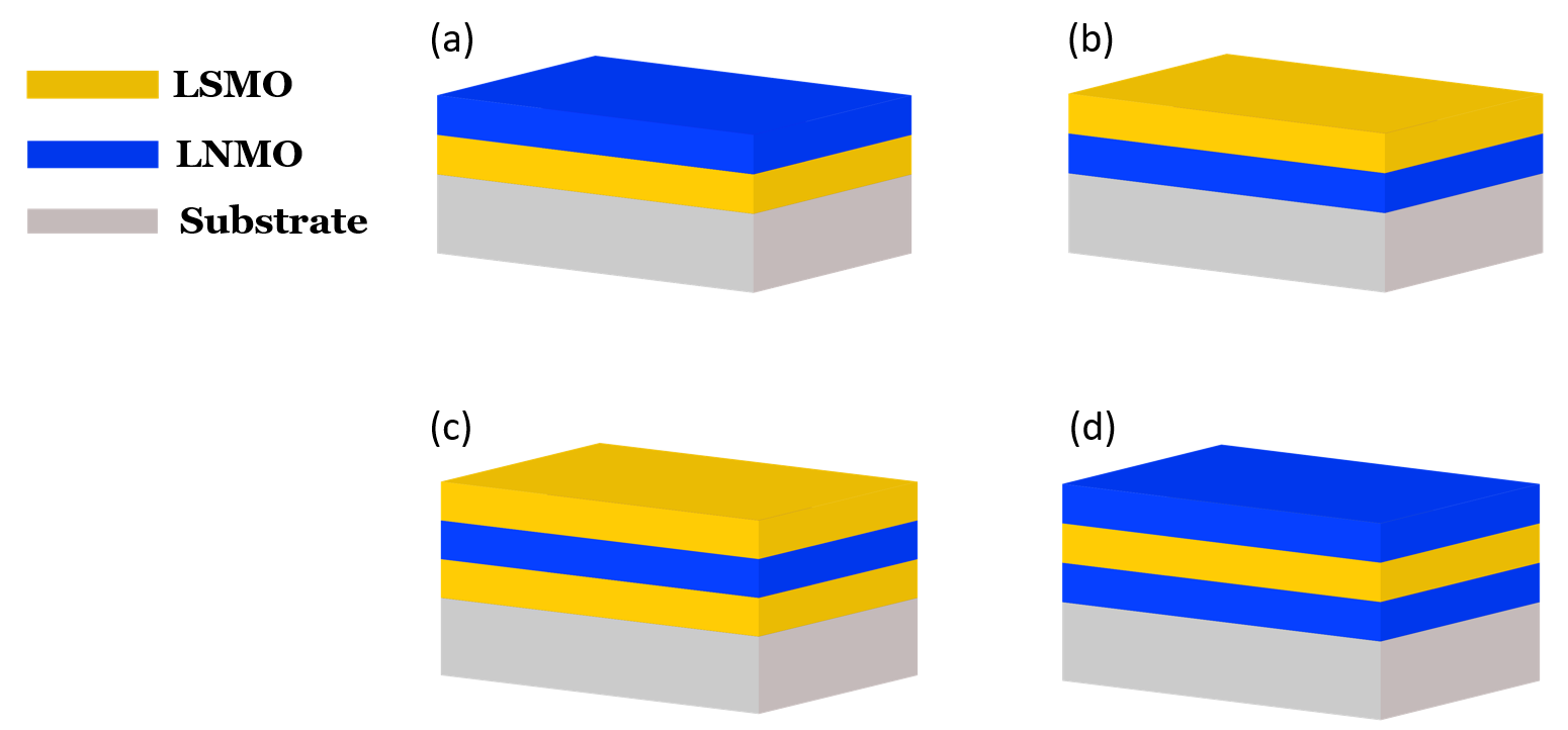
Room temperature x-ray diffraction (XRD) was performed using a high-resolution Bruker AXS D8-diffractometer with radiation in the configuration. The measurement of the magnetic properties are carried out using a Magnetic Property Measurement System (MPMS) from Quantum Design. In order to detect the small magnetic signals from thin films, magnetization measurements were performed using the reciprocating sample option (RSO) with an external magnetic field applied parallel to the surface of the samples. In this work, in order to determine the Arrott plots and the isothermal magnetic entropy changes (), the isothermal magnetization curves as a function of the applied field up to in the temperature range of with a temperature interval of are measured for all the samples. Figure 2 shows an example of isothermal magnetization measurements for a B – NS sample. As one may notice, all the magnetization curves show a negative slope at large field (Fig. 2 (a)) which originates from the diamagnetism of the substrate and the sample holder. As shown in Fig. 2 (b), the magnetization of layers which saturate very rapidly at low field can be clearly seen by removing this negative background. It should also be mentioned that the mass of the multilayers were estimated using the theoretical density of LSMO and LNMO, as well as the volume of the layers.


III Results and discussion
Figure 3 shows the XRD patterns of all samples from to close to the substrate’s Bragg peak. The XRD patterns of thick monolayers of LSMO and LNMO at the bottom of the figure show the proximity of their diffraction peaks. In these individual spectra, the single layers of LSMO and LNMO exhibit a central peak at and , respectively. In both cases, their position is in part defined by the impact of strain due to their lattice mismatch with the substrate shifting their angular position with respect to the bulk guo2013near; ettayfi2016structural. We are expecting strain to play also a role for thinner layers inserted in multilayers with additional shifts. Nevertheless, the growth conditions used for this work produce extremely smooth LSMO as revealed by the numerous Laue oscillations.
For the multilayers, all observed peaks can be assigned to the crystallographic planes. It is confirming their out-of-plane orientation and a smooth cube-on-cube growth. For bilayers, the LNMO diffraction peak for B – SN sits at a lower value of than in B – NS as its top LNMO layer is affected by the compressive strain from the bottom LSMO layer. In the supplemental material, we show the spectra close to the substrate’s Bragg peak. In this case, we observe Laue oscillations coming from LSMO and/or LNMO layers. The presence of these oscillations confirms the good crystalline quality of our samples with a well-defined interfaces. The top two spectra in Fig. 3 present the data for T – NSN and T – SNS trilayers. We notice the presence of three distinct peaks in the spectrum for T – NSN, where the peaks for the top and the bottom layers of LNMO coexist in the sample: their separation is the result of different strain experienced by both layers. In this particular case, we conclude in fact that the top LNMO layer is affected by a stronger compressive strain than the bottom one. Finally, the XRD spectrum for T – SNS shows only two diffraction peaks, one is associated to the middle LNMO layer, and two LSMO layers show a broad peak close to the substrate’s peak.
Atomic force microscopy (AFM) data (see supplemental material) show that the surface roughness on top of the monolayers, bilayers and trilayers is on the order of , and , respectively. In fact, variations of about over lateral distances of the order of for the monolayers indicate that the second and/or the third layers grow on top of a fairly smooth surface, resulting in well-defined interfaces between the layers.
In the next section the magnetic and magnetocaloric properties of bilayer and trilayer samples will be investigated in detail.

III.1 Bilayers
Figure 4 shows field-cooled (FC) magnetization measurements as a function of temperature at a fixed magnetic field of for bilayer samples. Both samples undergo two magnetic phase transitions from the ferromagnetic to the paramagnetic state. In the case of the B – NS sample, a first transition at roughly comes from the LNMO layer while the other at is related to the LSMO layer. The magnetic transition of LNMO at temperatures above confirms a high but incomplete level of cation ordering at the sites in the LNMO layer sitting directly on the substrate. For B – SN layout, the magnetic transition of the LSMO layer shifts at , while the transition temperature of LNMO sitting on top of LSMO shifts down to . The lower transition temperature of the LNMO layer in this configuration indicates a lower level of cation ordering than in the previous bilayer singh2010multiferroic. This difference in cation ordering level for LNMO in both bilayers is likely driven by the different strain fields experienced by the LNMO layer wu2018b; jin2016phase. Even the slight difference in the transition temperature of the LSMO layer in different bilayer configurations with shifts from in B – NS to in B – SN can be also attributed to the effect of strain dey2007effect; wang2013oxygen.
This set of bilayers demonstrates that we can change easily the level of cation ordering in LNMO and control the magnetic properties of layers just by changing the layout of the layers in bilayers, but also in more complex heterostructures. This feature provides an interesting avenue to tailor the magnetocaloric behavior close to room temperature, which will be discussed in detail later.

As it is known, MCE strongly depends on the nature of the magnetic phase transition. It should be noted that materials with a first-order magnetic phase transition usually show a large magnetic entropy change in a very narrow temperature range while their magnetic transition is usually accompanied by large thermal and magnetic hysteresis which neither of them are favorable for magnetic cooling systems phan2007review; smith2012materials. On the other hand, the broad magnetic phase transition and the reversible nature in second-order phase transition materials make them better suited for magnetic cooling systems. So, in order to get a deeper understanding of the nature of magnetic phase transition in our samples, the Arrott plots for the bilayers are derived from isothermal magnetization curves which are measured in the temperature range between under to . According to Banerjee’s criterion banerjee1964generalised, the negative or positive slope of Arrott plots indicate whether the magnetic phase transition is first or second order, respectively. The Arrott plots of the B – NS bilayer sample is depicted in Figure 5 as an example, and it clearly shows a positive slope for the entire temperature range confirming the existence of a second-order magnetic phase transition in our sample. Moreover, the transition temperature of magnetic materials can be extracted using the same plots arrott1957criterion. Based on the mean-field theory, Arrott plot curves near the transition temperature become straight lines crossing the origin. The inset of Fig. 5 shows the same Arrott plots near the highest transition temperature corresponding to LSMO for that B – NS sample. Similar plots can be found in the supplemental material for the other configurations. From this data, it was found that the highest transition temperature of B – NS and B – SN samples occur at , respectively. These transition temperatures from the LSMO layers are in close agreement with the M(T) measurements. Unfortunately, the lowest transition temperature of LNMO cannot be isolated out of these plots.

In order to determine , Maxwell’s relation linking the magnetic entropy change to the bulk magnetization (M), the temperature (T) and the external magnetic field (B) can be used through the following equation tishin2016magnetocaloric:
| (1) |
In both isothermal and isobaric conditions, the isothermal magnetic entropy change induced by a change in external magnetic field can then be written as:
| (2) |
Eq. 2 indicates that the magnetic entropy change is proportional to both the external field variation and the sharpness of a magnetic phase transition. Since magnetization measurements are usually made at discrete field and temperature intervals, can rather be computed using phan2007review:
| (3) |
where and are the magnetization value measured at temperatures and , under a magnetic field changing from to , respectively. Thus, Eq. 3 (and Eq. 2) evaluates the surface area between two isothermal magnetization curves measured at and (as presented in Fig. 2 (b)) with being their average.
The main scope of this work is to tailor a large and temperature independent magnetic entropy change over a wide temperature range. In order to achieve this goal and make a desirable magnetocaloric material, composite-like bilayer and trilayer structures are chosen as the main route. On top of that, it uses LNMO as a magnetic material with a tunable magnetic transition and combines it within a composite-like structure in the hope of getting a unique magnetocaloric feature. As discussed earlier, the magnetic properties of bilayer samples such as are affected by changing their layout. So, in this part we inspect to see how this change affects the magnetocaloric properties of bilayer samples.
The calculated isothermal magnetic entropy changes () as a function of temperature are shown in Figures 6 (a) and (b) for both bilayer samples under various magnetic field changes up to . Moreover, the magnetic entropy changes of the monolayers of LNMO and LSMO for are displayed in the background of Fig. 6 with light blue and grey, respectively. As expected, both bilayer samples exhibit two broad maxima in curves approaching the transition temperatures of each layer. In the B – NS sample (Fig. 6 (a)), these two maxima seen at are related to the of the cation ordered LNMO and the LSMO layers, respectively. The transition temperature of the LNMO layer almost coincides with that of the monolayer of LNMO with a at , confirming that the level of cationic ordering in this layer is not very much affected by the strain from the top LSMO layer. In comparison to the monolayer of LSMO in which the is at , the LSMO layer in the B – NS sample experiences a - shift in transition. The difference could originate from the epitaxial strain caused by the bottom LNMO layer leading to a change in the bond length and bond angle of Mn – O – Mn bonds in the octahedra. The maximum magnetic entropy changes which are attributed to ordered LNMO and LSMO layers are for a magnetic field change of . On the other hand, in the B – SN sample (Fig. 6 (b)), the maximum which is related to the transition of LNMO layer shifts down to , while the one related to the transition of LSMO increases to . The significant drop in the of LNMO can be attributed to the reduction of the cationic ordering level due to the increased epitaxial strain on the LNMO layer, which is in agreement with the trend observed in the XRD data (Fig. 3). Also, reaches a maximum value of for LNMO and LSMO layers under , respectively.
As noticed, both bilayer samples show a large magnetic entropy change which barely varies over a wide temperature range. The full width at half maximum is about for both samples (from to above room temperature at ). Unlike the other approaches used to tune the magnetic properties and especially the MCE such as doping or changing the growth conditions, this composite-like approach allows one to widen the magnetic entropy change without sacrificing much of the magnitude. In the next section we show how can be further improved in terms of intensity and temperature span by adding another layer to the composites structure. Of course, we will show that strain can be used to our advantage as was done with bilayers.


III.2 Trilayers
As seen in the previous section, we can take advantage of the sensitivity of cation ordering to strain of LNMO in multilayer samples just by changing the stacking order of the layers. This effect originates from different lattice mismatches between the layers and the substrate. It provides an opportunity to control the magnetic and magnetocaloric properties of more complex heterostructures and tailor a large MCE over a wide temperature range. As a proof of concept, trilayer samples with LNMO – LSMO – LNMO and LSMO – LNMO – LSMO configurations are compared.
Figure 7 shows field-cooled (FC) magnetization as a function of temperature under a fixed magnetic field of for both trilayer samples. As expected, T – NSN sample exhibits three magnetic phase transitions at roughly . This is confirmed in particular using the derivative as shown in the inset of Fig. 7. The first transition at comes from the top LNMO layer experiencing strain similar to that in the B – SN sample. The second magnetic transition at comes from the bottom LNMO layer in direct contact with the substrate as was observed in the B – NS bilayer. Finally, the transition at is related to the LSMO layer sitting between two LNMO, consistent also with its observed in the B – NS bilayer. In the other trilayer sample (T – SNS), we observe only two magnetic phase transitions in the M(T) curve at . The LSMO layers show a at and the middle LNMO layer has a at . This value of indicates that it has almost the same level of cationic ordering as what we have observed for LNMO in B – SN sample.
In a trilayer sample with two LNMO layers, we can have both disordered and highly ordered LNMO phases simultaneously in the sample from the top and bottom layers experiencing different strain fields. As a result, trilayer samples with the T – NSN configuration gives three different transitions which covers quite a large temperature range starting from . With an appropriate choice of thicknesses for each layer, one could get a temperature-independent table-top magnetic entropy change over a wide temperature range close to room temperature.

As mentioned before, one of the biggest advantage of SOMT materials is their small thermal and magnetic hysteresis. In Figure 8 (a), the magnetization as a function of magnetic field was measured for a T – NSN sample at the transition temperature of each layer and at . The sample saturates very quickly at low magnetic field, and also it exhibits a very low coercive field of at and this value decreases to roughly at (Fig. 8 (b)). The same is observed for the T – SNS sample (see supplemental material).


Magnetic isotherms measurements are carried out in the temperature range going from to determine Arrott plots and magnetic entropy changes for both trilayer samples. Similar to bilayers, an example of Arrott plots measurements for trilayers is shown in Figure 9. All vs. curves of the T – SNS sample show positive slopes in the entire temperature range which indicates that the sample undergoes a second-order magnetic phase transition. A similar trend can be observed in the Arrott plots of the other trilayer (T – NSN, see supplemental material). Furthermore, in order to determine the of the samples, the Arrott plots close to the transition temperature of T – SNS multilayer is depicted in the inset of Fig. 9. It is found that the transition of T – SNS and T – NSN samples occur at , respectively. As we saw in the bilayer samples, these two transitions are those of the LSMO layers in agreement with the M(T) measurements in Fig. 7.

Magnetic entropy changes as a function of temperature taken at different magnetic fields for the two trilayer samples are plotted in Figures 10 (a) and (b). At the transition temperature of each layer, there is a broad maximum in that comes from the magnetic phase transitions occurring at the transition temperatures of each layer. For instance, the T – SNS sample (Fig. 10 (a)) exhibits two peaks in curves at which correspond to the magnetic transition of LNMO and two LSMO layers, respectively. The maximum values of corresponding to LNMO and LSMO layers are for . As shown in Fig. 10 (b), the other trilayer sample (T – NSN) shows three peaks in curves due to the existence of different magnetic phases in two LNMO layers. They can be better observed for low applied field (). For this layer configuration, the peaks are located at which are related to the transition of disordered LNMO layer (the top layer), the cation-ordered LNMO layer (the bottom layer) and the LSMO middle layer, respectively. For , shows a maximum of that correspond to disordered LNMO, ordered LNMO and LSMO layers, respectively.
It must be emphasized that the large magnetic entropy changes with a wide operating temperature range ( = ) which go slightly above room temperature would make these multilayer composites an interesting candidate for magnetic cooling systems at room temperature. In addition, both trilayer samples show a fairly flat and temperature-independent within the mid-range temperature which can extend over under (Figs. 10). This temperature independent over a wide temperature window would make these two trilayer samples suitable candidates for AMR refrigeration franco2018magnetocaloric. Moreover, with an appropriate choice of thicknesses for each layer (for example a bit thicker for LSMO) one could likely generate a constant from .


A useful tool which allows usually to compare the cooling performances of magnetocaloric materials is the relative cooling power . is the amount of heat transfer between the cold and hot reservoirs in one refrigeration cycle and it is defined as:
| (4) |
RCP is not only considering the amplitude of the magnetic entropy change , but it also takes into account the working temperature range which is a key parameter in magnetic cooling systems. is mostly used for materials with a single transition which have a fairly symmetric peak in curves. However, in the case of composites and materials with more than one transition, refrigerant capacity is usually employed matte2018tailoring; zhou2018table. is specified as the area under the curve of between the temperatures which correspond to half maximum gschneidner1999recent:
| (5) |
Figure 11 presents the values as a function of magnetic field for all four samples and also that of gadolinium as a reference to compare with our samples. All samples show a relatively large with an almost linear magnetic field dependence. The values of reach for B – SN, B – NS, T – SNS and T – NSN under a magnetic field of , respectively. By comparing with Gadolinium as a reference dan1998magnetic, it can be seen that the value of for T – NSN sample is about of Gd for . All the values of and for our samples under different magnetic fields are listed in Table 1. Among other families with comparable to Gd, such as shamba2013enhancement; shamba2011reduction and provenzano2004reduction compounds, our multilayer samples have additional advantages over other candidates such as wide working temperature range and a second order magnetic phase transition. Our results confirm that the composite approach combining metals oxides such as manganites and double perovskites is a promising path to produce performant cooling devices based on the magnetocaloric effect.

| (6) |
| () | () | ||||||
|---|---|---|---|---|---|---|---|
| Sample | |||||||
| B – SN | 0.62 | 1.33 | 1.76 | 106.82 | 273.23 | 380.62 | |
| B – NS | 0.57 | 1.35 | 1.80 | 106.31 | 263.81 | 362.39 | |
| T – SNS | 0.68 | 1.50 | 2.03 | 104.91 | 258.61 | 351.14 | |
| T – NSN | 0.70 | 1.63 | 2.21 | 136.61 | 334.57 | 455.82 | |
IV Conclusion
In this work, we obtain a large and almost temperature independent magnetocaloric effect extending from up to room temperature in multilayer composites of LNMO and LSMO. We take advantage of the sensitivity of cationic ordering to strain in LNMO layers to achieve multilayers with multiple magnetic transitions. For this purpose, two series of bilayer samples with different layouts of LSMO – LNMO and LNMO – LSMO, and two series of trilayer samples with layouts of LSMO – LNMO – LSMO and LNMO – LSMO – LNMO are prepared. All the samples show a large over a wide temperature range, as large as , which extends above room temperature. The maximum value of in the trilayer samples is found to be under a magnetic field change of in T – SNS and T – NSN samples, respectively. Moreover, the trilayer samples reveal an almost temperature independent magnetic entropy change that can extend over a large temperature range of . The refrigerant capacity reaches a maximum value of for in T – SNS and T – NSN samples, respectively. These large values of in our composite-like multilayers are comparable to Gd and other reference materials. Our results demonstrate that a composite route to design new materials for magnetic cooling systems is a promising path.
Acknowledgment
The authors thank B. Rivard, S. Pelletier and M. Dion for technical support. The authors would also like to thank P. Brojabasi for preparing the initial samples. This work is supported by the Natural Sciences and Engineering Research Council of Canada (NSERC) under grant RGPIN-2018-06656, the Canada First Research Excellence Fund (CFREF), the Fonds de Recherche du Québec - Nature et Technologies (FRQNT) and the Université de Sherbrooke. M.B. acknowledges the financial support from the International University of Rabat.
References
- 1 Balli, M., Jandl, S., Fournier, P., and Kedous-Lebouc, A. Appl. Phys. Rev. 4(2), 021305 (2017).
- 2 GschneidnerJr, K. A., Pecharsky, V., and Tsokol, A. Rep. Prog. Phys. 68(6), 1479 (2005).
- 3 Weiss, P. and Piccard, A. J. Phys. Theor. Appl. 7(1), 103–109 (1917).
- 4 Brown, G. J. Appl. Phys. 47(8), 3673–3680 (1976).
- 5 Pecharsky, V. K. and Gschneidner Jr, K. A. Phys. Rev. Lett. 78(23), 4494 (1997).
- 6 Xu, Z., Lin, G., and Chen, J. J. Alloys Compd. 639, 520–525 (2015).
- 7 Balli, M., Rosca, M., Fruchart, D., and Gignoux, D. J. Magn. Magn. Mater. 321(2), 123–125 (2009).
- 8 Fujieda, S., Fujita, A., and Fukamichi, K. Appl. Phys. Lett. 81(7), 1276–1278 (2002).
- 9 Fujita, A., Fujieda, S., Fukamichi, K., Mitamura, H., and Goto, T. Phys. Rev. B 65(1), 014410 (2001).
- 10 Tokura, Y. and Tomioka, Y. J. Magn. Magn. Mater. 200(1-3), 1–23 (1999).
- 11 Phan, M.-H. and Yu, S.-C. J. Magn. Magn. Mater. 308(2), 325–340 (2007).
- 12 Mira, J., Rivas, J., Hueso, L., Rivadulla, F., and Lopez Quintela, M. J. Appl. Phys. 91(10), 8903–8905 (2002).
- 13 Balli, M., Fournier, P., Jandl, S., Truong, K., and Gospodinov, M. J. Appl. Phys. 116(7), 073907 (2014).
- 14 Brahiti, N., Abbasi Eskandari, M., Balli, M., Gauvin-Ndiaye, C., Nourafkan, R., Tremblay, A.-M., and Fournier, P. J. Appl. Phys. 127(11), 113905 (2020).
- 15 Kobayashi, K.-I., Kimura, T., Sawada, H., Terakura, K., and Tokura, Y. Nature 395(6703), 677–680 (1998).
- 16 Anderson, P. W. Solid State Phys. 14, 99–214 (1963).
- 17 Kanamori, J. J. Phys. Chem. Solids 10(2-3), 87–98 (1959).
- 18 Singh, M., Truong, K., Jandl, S., and Fournier, P. J. Appl. Phys. 107(9), 09D917 (2010).
- 19 Iliev, M., Gospodinov, M., Singh, M., Meen, J., Truong, K., Fournier, P., and Jandl, S. J. Appl. Phys. 106(2), 023515 (2009).
- 20 Bull, C., Gleeson, D., and Knight, K. J. Phys.: Condens. Matter 15(29), 4927 (2003).
- 21 Matte, D., de Lafontaine, M., Ouellet, A., Balli, M., and Fournier, P. Phys. Rev. Applied 9(5), 054042 (2018).
- 22 Rebello, A., Naik, V., and Mahendiran, R. J. Appl. Phys. 110(1), 013906 (2011).
- 23 Zhong, X., Shen, X., Mo, H., Jiao, D., Liu, Z., Qiu, W., Zhang, H., and Ramanujan, R. Mater. Today Commun. 14, 22–26 (2018).
- 24 Zhang, Y., Yang, Y., Xu, X., Geng, S., Hou, L., Li, X., Ren, Z., and Wilde, G. Sci. Rep. 6(1), 1–9 (2016).
- 25 Tian, H., Zhong, X., Liu, Z., Zheng, Z., and Min, J. Mater. Lett. 138, 64–66 (2015).
- 26 Guo, Y., Shi, L., Zhou, S., Zhao, J., and Liu, W. Appl. Phys. Lett. 102(22), 222401 (2013).
- 27 Ettayfi, A., Moubah, R., Boutahar, A., Hlil, E., and Lassri, H. J Supercond Nov Magn 29(1), 133–138 (2016).
- 28 Wu, S.-Q., Cheng, S., Lu, L., Liu, M., Jin, X.-W., Cheng, S.-D., and Mi, S.-B. Sci. Rep. 8(1), 1–9 (2018).
- 29 Jin, X.-W., Lu, L., Mi, S.-B., Liu, M., and Jia, C.-L. Appl. Phys. Lett. 109(3), 031904 (2016).
- 30 Dey, P., Nath, T., and Taraphder, A. Appl. Phys. Lett. 91(1), 012511 (2007).
- 31 Wang, B., You, L., Ren, P., Yin, X., Peng, Y., Xia, B., Wang, L., Yu, X., Mui Poh, S., Yang, P., et al. Nat. Commun. 4(1), 1–7 (2013).
- 32 Smith, A., Bahl, C. R., Bjørk, R., Engelbrecht, K., Nielsen, K. K., and Pryds, N. Adv. Energy Mater. 2(11), 1288–1318 (2012).
- 33 Banerjee, B. Physics Letters 12(1), 16–17 (1964).
- 34 Arrott, A. Phys. Rev. 108(6), 1394 (1957).
- 35 Tishin, A. M. and Spichkin, Y. I. The magnetocaloric effect and its applications. CRC Press, (2016).
- 36 Franco, V., Blázquez, J., Ipus, J., Law, J., Moreno-Ramírez, L., and Conde, A. Prog. Mater. Sci. 93, 112–232 (2018).
- 37 Zhou, L., Tang, Y., Chen, Y., Guo, H., Pang, W., and Zhao, X. J. Rare Earths 36(6), 613–618 (2018).
- 38 Gschneidner Jr, K., Pecharsky, V., Pecharsky, A., and Zimm, C. Materials Science Forum 315, 69–76 (1999).
- 39 Dan’Kov, S. Y., Tishin, A., Pecharsky, V., Gschneidner, K., et al. Phys. Rev. B 57(6), 3478 (1998).
- 40 Shamba, P., Zeng, R., Wang, J., Campbell, S., and Dou, S. J. Magn. Magn. Mater. 331, 102–108 (2013).
- 41 Shamba, P., Debnath, J., Zeng, R., Wang, J., Campbell, S. J., Kennedy, S., and Dou, S. J. Appl. Phys. 109(7), 07A940 (2011).
- 42 Provenzano, V., Shapiro, A. J., and Shull, R. D. Nature 429(6994), 853–857 (2004).
Supplemental material

![[Uncaptioned image]](2211.02715v1/LSMO_afm.png)
![[Uncaptioned image]](2211.02715v1/LNMO_afm.png)
![[Uncaptioned image]](2211.02715v1/B_NS_afm.png)
![[Uncaptioned image]](2211.02715v1/B_SN_afm.png)
![[Uncaptioned image]](2211.02715v1/T_NSN_afm.png)

![[Uncaptioned image]](2211.02715v1/B_SN_iso.png)
![[Uncaptioned image]](2211.02715v1/T_SNS_iso.png)

![[Uncaptioned image]](2211.02715v1/M_H_SNS_a.png)


