Discovery of a double sequence of blue straggler stars in the core-collapsed globular cluster NGC 6256Journal: ApJ

Blue straggler stars (BSSs) are an exotic population of stars located in a more luminous and bluer region than main-sequence (MS) turn-off (TO) in the color-magnitude diagram (CMD) of stellar systems (Sandage 1953; Ferraro et al. 1997; Ferraro et al. 2003b; Ferraro et al. 2012; Ferraro et al. 2018; Piotto et al. 2004; Leigh et al. 2007; Boffin et al. 2015, e.g.,). They are core hydrogen-burning stars more massive (Fiorentino et al. 2014; Raso et al. 2019, e.g.,) than MS-TO objects and thought to be the outcome of two main processes: mass-transfer and/or coalescence in binary systems (hereafter, MT-BSSs; McCrea 1964), and (2) direct stellar collisions (COL-BSSs; Hills & Day 1976). Other processes, such as merger of close binary systems, possibly induced by Kozai-Lidov mechanisms in hierarchical triple systems, can also play a role in generating BSSs (Perets & Fabrycky 2009). While the formation channels requiring binary systems are common in all stellar environments and dominant in low-density conditions, such as the peripheries of globular clusters (GCs), open clusters, dwarf galaxies and the Galactic field, the collisional channel requires very high-density environments. Hence, the inner cores of GCs offer the most favorable conditions for direct stellar collisions to occur, although the MT channel is considered the most prolific one (Davies et al. 2004; Knigge et al. 2009; Leigh et al. 2013, e.g.). Since BSSs are ubiquitous found in all GCs and are more massive than the average (Ferraro et al. 2018; Rain et al. 2021, e.g.), they are used as powerful tools to study star cluster internal dynamics (Ferraro et al. 2012; Ferraro et al. 2018; Ferraro et al. 2019; Ferraro et al. 2020; Alessandrini et al. 2016; Lanzoni et al. 2016; Dresbach et al. 2022, e.g.). In particular, Ferraro et al. 2018 studied about one third of the entire GC population in our Galaxy and found a tight correlation between the number of relaxation times suffered by each cluster since formation ($N_{\rm relax}$) and the value of the $A^{+}_{rh}$ parameter. The latter is defined as the area between the cumulative radial distribution of BSSs and that of a reference population (such as MS, giant and horizontal branch stars), within a half-mass radius from the center of the system (Alessandrini et al. 2016). Its value thus measures the level of BSS central segregation with respect to “standard” (lighter) stars, which progressively increases while the host cluster dynamically evolves. Large values of $A^{+}_{rh}$ are therefore measured for GCs in late stages of their dynamical evolution, while small values (down to zero) are found in dynamically young systems, where dynamical friction has not been effective yet in segregating BSSs toward the center.

The distinction between BSSs formed through MT and collision would provide useful information about the collision rate of the cluster, the fraction of binaries and their impact on internal dynamics, and also insights on the formation and evolution of these exotic objects. Unfortunately, BSSs formed through different channels are hardly distinguishable from their photometric properties. The only exception known so far could be the presence of two distinct BSS sequences in the CMD of post core-collapse (PCC) clusters¹¹ 1 The core-collapse is a characteristic phase of the internal dynamical evolution of collisional stellar systems. It is the result of the continuous kinetic energy transfer from the inner regions to the outskirts that leads to a runaway contraction of the core, with a substantial increase of its density. PCC clusters are commonly recognized from the presence of a steep power-law cups in the innermost portion of the density profile (Meylan & Heggie 1997).. This feature has been first discovered in the GC M30 (Ferraro et al. 2009), and it has then been identified in a few additional systems: NGC 362 (Dalessandro et al. 2013), NGC 1261 (Simunovic et al. 2014, but see Raso et al. 2020), and M15 (Beccari et al. 2019)²² 2 A detection of a double BSS sequence in the Large Magellanic Cloud GC NGC 2173 has been claimed by (Li et al. 2018), but this is most likely an artifact of field star contamination (Dalessandro et al. 2019a; Dalessandro et al. 2019b). All these clusters show in the CMD a narrow sequence of blue BSSs, separated through a clear-cut gap from a more scattered red BSS population. The red sparse sequence is not reproducible with collisional isochrones (Sills et al. 2009) of any age, while it is in good agreement with the CMD location of MT-BSS models (Xin et al. 2015), thus suggesting that it is likely populated by BSSs formed through the MT channel. On the other hand, the blue sequence is inconsistent with the MT-BSS models of Xin et al. 2015 and is well reproduced by collisional isochrones, thus suggesting that it is likely populated by COL-BSSs. Interestingly, Monte Carlo simulations by Jiang et al. 2017 show that the blue sequence could be also contaminated by MT-BSSs. However, its narrowness and the clear-cut separation from the red sequence appear to be inconsistent with a formation from MT activity in binary systems, which extends over long time scales. On the other hand, the results obtained by Jiang et al. 2017 could explain the presence of the few W-Uma stars (contact binaries) detected along the blue sequence of M30 and NGC 362 (Ferraro et al. 2009; Dalessandro et al. 2013). The narrowness of the blue sequence suggests that it is more likely composed of a population of coeval BSSs with different masses, all formed over a relatively short period of time. Based on this evidence, Ferraro et al. 2009 suggested that the origin of the observed blue sequence is related to the core-collapse (CC) event which enhanced the cluster collision rate in inner regions over a short time scale. This working hyphothesis was later confirmed by numerical simulations specifically performed to reproduce the bimodal BSS distribution of M30 (see Portegies Zwart 2019). In addition, as a matter of fact, the three clusters where the double BSS sequence has been firmly identified so far (i.e. M30, NGC 362 and M15) already experienced the CC phase (see Harris 1996, 2010 edition). In light of all this, Ferraro et al. 2009 suggested that the properties of the blue narrow sequence could be also used to date back the CC epoch: as the MS-TO luminosity is a proxy of the cluster age, so the luminosity of the blue BSS sequence (or its extension in luminosity) can provide an estimate of the epoch when the system experienced a significant enhancement of its collision rate, which triggered the formation of COL-BSSs that we now observe aligned in the CMD.

In this paper we present the discovery of a double sequence of BSSs in the GC NGC 6256. This is a dense cluster ($\log{\rho_{0}}\approx 5.9$ in units of $M_{\odot}$ pc^-3; Baumgardt & Hilker 2018) located in the Galactic bulge, at a distance of 6.8 kpc from the Sun (Cadelano et al. 2020b) and characterized by a relatively low metal content compared to typical bulge GCs ([Fe/H]$=-1.6$; Vásquez et al. 2018). In Cadelano et al. 2020b, we applied a well-tested procedure (Pallanca et al. 2019; Pallanca et al. 2021, see) to quantify the differential reddening affecting the cluster and we derived a high-resolution exctiction map (see Figure 3 in Cadelano et al. 2020b): color excess variations as large as $\delta E(B-V)\sim 0.51$ mag were measured in the relatively small $160\arcsec\times 160\arcsec$ field of view (FOV) sampled by the adopted data-set. The differential reddening corrected CMD allowed the authors to derive an age of $13\pm 0.5$ Gyr. The analysis of the CMD also revealed a severe contamination by field interlopers along the cluster’s main evolutionary sequences.

In the comprehensive analysis of GC surface brightness profiles by Trager et al. 1993; Trager et al. 1995, NGC 6256 is classified as a PCC cluster, due to the presence of a central surface brightness cusp. However, the cluster structural properties based on surface brightness profiles suffer from the so-called “shot-noise bias”, due to the stochastic and sparse presence of luminous stars, which can significantly displace the surface brightness peak from the true location of the cluster gravitational center and alter the shape of the surface brightness profile with respect to the true density distribution (Noyola & Gebhardt 2006; Cadelano et al. 2017; Lanzoni et al. 2019, see, e.g.).

Recently, Cohen et al. 2021 determined the cluster’s structural parameters from the star count density profile. They derived a cluster gravitational center by fitting ellipses to the isodensity contours, and found a value in agreement, within the uncertanties, with the one quoted in Cadelano et al. 2020b, which was calculated through iterative re-centering of the stellar average coordinates. They also determined the cluster’s structural parameters through King 1966 model fitting of the density profiles obtained by combining the same high-resolution observations used throughout this work (see Section II) to sample the central regions, with Gaia DR2 photometry (Gaia Collaboration et al. 2018) to sample the cluster’s outskirts. The authors discuss that the best-fit model is unable to properly reproduce the observed stellar density in the cluster’s innermost regions, which is expected in the case of a very dynamically evolved and core-collapsed cluster.

This paper is structured as follows: in Section II we introduce the adopted data-set and the data reduction procedures; in Section III we determine the cluster’s stellar density profile and investigate its dynamical status; in Section IV we discuss the proper motion (PM) analysis and present the discovery of a double sequence of BSSs. Finally, we summarize the result and draw our conclusions in Section V.

High-resolution data-set: this work is mainly based on two data-set of optical images obtained with the Hubble Space Telescope (HST). The first data-set was obtained using the UVIS channel of the Wide Field Camera 3 (WFC3) under GO 11628 (PI: Noyola). It consists of 3 images acquired with the F555W filter and exposure time of 360 s, and 3 images in the F814W filter with exposure time of 100 s. The adopted procedures of data reduction, astrometry and calibration are described in detail in Cadelano et al. 2020b, where it is also discussed the determination of a high-resolution differential reddening map in the direction of the system. The second data-set was obtained under GO 15065 (PI: Cohen) using the Wide Field Camera (WFC) of the Advanced Camera for Surveys (ACS). It consists of 4 images acquired with the F606W filter with exposure time of 498 s and 4 images acquired with the F814W filter with exposure time of 509 s. The data reduction was performed using a standard approach with DAOPHOT and ALLFRAME packages (Stetson 1987; Stetson 1994), in a similar way as described in Cadelano et al. 2020b in the case of the WFC3 data-set. The FOVs of the two HST data-sets overlap and are separated by a temporal baseline of 3605 days ($\sim 10$ yr), thus allowing the measure of stellar PMs (see Section IV.1). All the HST magnitudes used hereafter throughout the work are corrected for the effects of differential reddening.

Wide-field data-set: to dermine the stellar density profile along the entire radial extension of the cluster, we complemented the high-resolution HST data, with a set of wide-field near-infrared images obtained as a part of the VVVX survey (Minniti 2016). This data-set was acquired with the VISTA InfraRed CAMera (VIRCAM) mounted on the VISTA-ESO telescope. It is composed of 2 images obtained with the J filter and exposure time of 120 s, 1 image with the H filter and exposure time of 48 s and, finally, 1 image with the Ks filter and exposure time of 16 s. Also in this case, the data reduction was performed using a standard approach suitable for ground-based observations with DAOPHOT and ALLFRAME packages (Cadelano et al. 2020a, see e.g.). The resulting catalog was astrometrized using the stars in common with the Gaia Data Release 3 (DR3) catalog (Gaia Collaboration, 2022, in preparation) and the instrumental magnitudes were calibrated using the stars in common with the catalog by Valenti et al. 2007, obtained with the same filters and in an overlapping region of the sky.

The map of the FOVs covered by all the data-sets used in this work is reported in Figure 1, while the corresponding CMDs are shown in Figure 2.

PCC clusters are typically characterized by the presence of a central density cusp usually shaped like a power-law, rather than the flat density core behavior predicted by King 1966 models and typically observed in less dynamically evolved GCs (Ferraro et al. 2003a; Lanzoni et al. 2007; Vesperini & Trenti 2010; Dalessandro et al. 2013; Miocchi et al. 2013; Zocchi et al. 2016, e.g.,). Based on the shape of its surface density distribution, NGC 6256 has been classified as a PCC system (Trager et al. 1993; Trager et al. 1995). In this section, we determine the cluster’s density profile from star counts to accurately estimate its structural properties and reliably confirm its core-collapsed nature.

We adopted the gravitational center derived in Cadelano et al. 2020b: $\alpha=16^{\rm h}59^{\rm m}32.668^{\rm s}$ and $\delta=-37^{\circ}07\arcmin 15.139\arcsec$, with an uncertainty of $\sim 0.4\arcsec$. As discussed in many previous papers (Ferraro et al. 1999; Ferraro et al. 2003a; Ibata et al. 2009; Lanzoni et al. 2007, see) the accurate determination of the center of gravity is crucial in order to properly characterize the star density profile, especially in high density clusters. The projected stellar density profile has been determined following the procedure fully described in Miocchi et al. 2013. To sample the inner $\sim 100\arcsec$, we used the WFC3 data-set. For the cluster’s outer regions, we used the wide-field VIRCAM data-set. The choice of using a near-IR data-set, instead of the publicly available Gaia DR3 catalog, is motivated by the fact that NGC 6256 is located in a region of the sky severely affected by differential reddening (Cadelano et al. 2020b, see). Hence, the adoption of a catalog of stars based on optical photometry, such as the Gaia one, could introduce significant alterations of the density profile with respect to its true shape, and thus lead to a wrong determination of the cluster structural parameters (see the case of M71 discussed in Cadelano et al. 2017).

In the case of the region sampled by the HST data-set, we divided the FOV into 12 concentric annuli out to $120\arcsec$ from the cluster’s center, each one divided into four sub-sectors. For each sub-sector, we then counted the number of stars having magnitude $15.5<m_{\rm F814W}<19.8$ (to avoid possible biases due to saturation and incompleteness of the brightest and faintest stars, respectively) and divided it by the sampled area. The resulting density in each annulus is the mean of the values measured in each sub-sector and the uncertainty is the standard deviation. We repeated the same procedure for the VIRCAM wide-field data-set, dividing the FOV in 8 concentric annuli from $38\arcsec$ out to $450\arcsec$ from the cluster’s center, and considering only stars having magnitude $11.5<K<16.5$. The three innermost radial bins ($38\arcsec<r<120\arcsec$) are also sampled with HST catalog and thus they have been used to vertically rescale the external (VIRCAM) profile to match the inner (HST) one. The resulting density profile is shown in Figure 3 (empty circles). The apparent external flattening is due to the Galactic field contribution, which is negligible with respect to the cluster density in the inner regions, but becomes dominant at large distances from the center. The average of the three most external points in linear (instead of logarithmic) units has been adopted as Galactic field density, and then subtracted from the observed distribution to obtain the background-decontaminated density profile of NGC 6256 (filled circles in Figure 3). The density profile clearly shows a progressive increase, instead of a flat behavior, toward the cluster center, which is the typical feature expected for a core-collapsed GC.

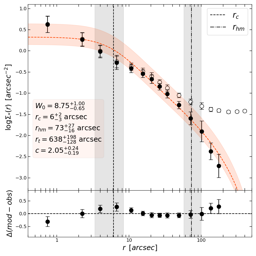
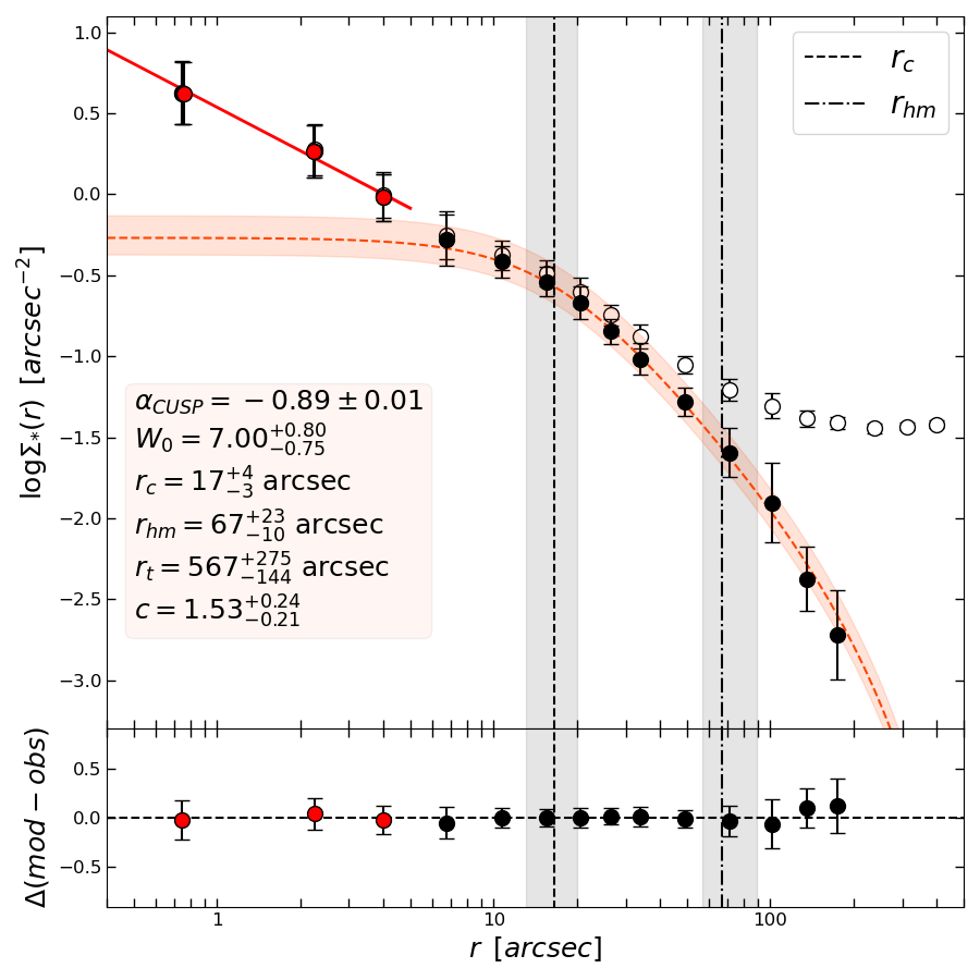
The density profile has been obtained using only TO, sub-giant and red-giant stars, which approximately have the same mass. Therefore, the cluster’s structural parameters have been derived by fitting the observed profile with a single-mass King 1966 model, assuming spherical symmetry and orbital isotropy. Following Raso et al. 2020, we performed the fit using a Markov Chain Monte Carlo approach by means of the emcee package (Foreman-Mackey et al. 2013; Foreman-Mackey et al. 2019). We assumed uniform priors on the parameters of the fit (i.e. the King concentration parameter $c$, the core radius $r_{c}$, and the value of the central density). Therefore, the posterior probability distribution functions are proportional to the likelihood $\mathscr{L}=\exp{(-\chi^{2}/2)}$, where the $\chi^{2}$ statistic is calculated between the measured density values and those predicted by the whole family of adopted models. As typically found for core collapsed GCs (Ferraro et al. 2003a; Zocchi et al. 2016, e.g.,), the resulting best-fit model (red dashed curve in the left-hand panel of Figure 3) clearly fails in properly reproducing the observations, and it is characterized by a value of the concentration parameter $c$ larger than 2. Instead, a very good King model fitting is obtained if the three innermost points ($r<5\arcsec$) are excluded from the analysis (red dashed curve in the right-hand panel of Figure 3). In turn, the evident central density cusp is well reproduced by a straight line, with a steep slope $\alpha_{\rm CUSP}=-0.89$ (red solid line in the figure). This is indeed the typical behavior of a PCC cluster (Vesperini & Trenti 2010, e.g.). The main structural parameters obtained from best-fit King model are also labelled in the figures, where $W_{0}$ is the model dimensionless potential, $r_{hm}$ is the 3D half-mass radius, and $r_{t}$ is the truncation or tidal radius. Figure 4 compares the density profile obtained in this work (black circles) with that determined through a very similar procedure by (Cohen et al. 2021, grey circles), vertically rescaled to match our data using an average density difference value. The two profiles are in overall good agreement, the main difference being that we sample a larger radial extension, both toward the center and in the periphery, with the density that keeps increasing in the innermost bin, as expected in the presence of a power-law cusp. This difference is likely due to different adoptions of the magnitude selection and slightly different coordinates of the cluster center. Nevertheless, the structural parameters derived here and in Cohen et al. (2021) are in agreement within $\sim 1-2\sigma$ errors.

The shape of the density profile clearly indicates that NGC 6256 is in a very advanced stage of its dynamical evolution, having already experienced the CC phase. To independently and more quantitatively investigate the dynamical status of this system, we analyzed the properties of the BSS population, which are known to act as a “dynamical clock” Ferraro et al. 2012; Ferraro et al. 2018; Ferraro et al. 2019; Ferraro et al. 2020; Lanzoni et al. 2016). However, NGC 6256 suffers from severe contamination from Galactic interlopers (Cadelano et al. 2020b), and a solid characterisation of the BSS population first requires a proper distinction between cluster’s members and field objects. Unfortunately, due to crowding, large extinction and distance, the kinematic information provided by the Gaia DR3 can be used only for the brightest portion of the red giant branch. Therefore, we took advantage of the large temporal baseline between the two HST data-sets to perform the PM analysis of the stars in common between the two epochs. A similar, independent analysis was also performed by Cohen et al. 2021.

In this paper we have performed a detailed photometric investigation of the bulge GC NGC 6256, also taking advantage of HST multi-epoch data to measure relative PMs in the inner region of the system for the accurate decontamination of the CMD from field stars. The analysis demonstrated that this GC is in a very advanced stage of dynamical evolution. In fact, the observed stellar density profile cannot be properly reproduced by a King model, and shows a steep power-law cusp with a slope of $-0.89$ in the innermost $\sim 5\arcsec$. This is the typical behavior expected for a cluster that already experienced CC (Bhat et al. 2022, see e.g.). A very advanced dynamical stage is also suggested by the value of the $A^{+}$ parameter (Alessandrini et al. 2016), measuring the level of BSS central segregation, with respect to lighter (MS-TO and giant) stars. As shown in Fig. 9, NGC 6256 well follows the same trend between $A^{+}$ and $N_{\rm relax}$ traced by $\sim 1/3$ of the entire Galactic GC population (Ferraro et al. 2018, from), and it locates in region of the diagram occupied by PCC clusters (diamonds).

The analysis also showed that the BSS population of NGC 6256 draws a well-defined narrow blue sequence (corresponding to what expected for a sub-population of BSSs with different masses generated over a relatively short time scale), and a more sparse red sequence. This is similar to what observed in other PCC clusters (M30, NGC 362, M15), where it has been interpreted (Ferraro et al. 2009, e.g.) as the manifestation of the two main BSS formation channels: the blue sequence should be originated mainly by collisions over a short time-scale, while the red sequence derives from a continuous formation process (Portegies Zwart 2019, see also), as expected in the case of MT-generated BSSs. Indeed, the comparison with collisional models from Sills et al. 2009 computed for a metallicity appropriate for NGC 6256 provides a very good match to the observations: the narrow blue sequence is well reproduced by a collisional isochrone of 1 Gyr, thus suggesting that, approximately 1 Gyr ago, a short-lasting event occurred and promoted the formation of a population of collisional BSSs, which currently represents $\sim 60\%$ of the entire BSS cluster content. The fact that NGC 6256 is a PCC system naturally yields to the conclusion that the blue sequence was originated by the increased collision rate during the CC phase. Based on analogous considerations, Ferraro et al. 2018 and Dalessandro et al. 2013 concluded that M30 experienced CC approximately 2 Gyr ago, and NGC 362 reached this phase of dynamical evolution more recently, about 0.2 Gyr ago. In the case of M15, the blue sequence is further separated in two different branches: the main one extends up to 2.5 mag above the MS-TO and is nicely reproduced by a $\sim 2.2$ Gyr collisional isochrone, while the second is $\sim 1$ mag less extended in the CMD and reproduced by a $\sim 5.5$ Gyr collisional isochrone (Beccari et al. 2019). The authors suggest that such a complex feature could be the result of two distinct events of high collisional activity: the first one is the cluster CC, occurred about 5.5 Gyr ago, and the second and more recent one corresponds to a core oscillation during the PCC evolution (see Figure 9 in Beccari et al. 2019). Intriguingly, the CMD positions of the two brightest BSSs along the blue sequence of NGC 6256 are consistent with a 0.1 Gyr collisional isochrone, thus possibly indicating the epoch of the last relevant re-collapse during the PCC gravothermal oscillation phase, similarly to the case of M15.

Of course, the photometric separation of the two kinds of BSSs in the CMD is not completely stringent. In fact, while MT-BSSs are unable to produce blue sequences as narrow and well-defined as observed, recent MT models (Jiang et al. 2017) demonstrate that some of them can “contaminate” the blue region of the CMD. This is indeed consistent with the presence of W-Uma variables identified along the blue sequence of M30 (Ferraro et al. 2009) and NGC 362 (Dalessandro et al. 2013), and possibly also in NGC 6256, where hints of photometric variability have been found for two blue BSSs (see Figure 8). On the other hand, also collisional BSSs that were born along the blue sequence cross the red sequence region during their natural evolution. However, the possibility of observing a collisional BSS during its evolution through the red portion of the CMD is low (for instance, a $1.1M_{\odot}$ collisional BSS originated by a $0.5M_{\odot}+0.6M_{\odot}$ collision spends approximativel 2 Gyr along the blue sequence, and only a few $10^{8}$ yr crossing the red strip).

The analysis discussed in this paper for NGC 6256, together with previous results for other PCC and “normal” GCs (Ferraro et al. 2009; Ferraro et al. 2018; Dalessandro et al. 2013; Beccari et al. 2019, e.g.), provide excellent examples of the potential prediction power of the BSS distribution in tracing the dynamical history of stellar systems. On the one hand, the segregation level of BSSs is a very powerful empirical way for the classification of GCs in terms of their level of internal dynamical evolution. On the other hand, the morphology of the BSS sequence in the CMD can be used to trace the time-scale of dynamical evolution during and after CC.

References

- Alessandrini et al. (2016) Alessandrini, E., Lanzoni, B., Ferraro, F. R., Miocchi, P., & Vesperini, E. 2016, ApJ, 833, 252, doi: 10.3847/1538-4357/833/2/252
- Baumgardt & Hilker (2018) Baumgardt, H., & Hilker, M. 2018, MNRAS, 478, 1520, doi: 10.1093/mnras/sty1057
- Beccari et al. (2019) Beccari, G., Ferraro, F. R., Dalessandro, E., et al. 2019, ApJ, 876, 87, doi: 10.3847/1538-4357/ab13a4
- Bellini et al. (2011) Bellini, A., Anderson, J., & Bedin, L. R. 2011, PASP, 123, 622, doi: 10.1086/659878
- Bellini et al. (2014) Bellini, A., Anderson, J., van der Marel, R. P., et al. 2014, ApJ, 797, 115, doi: 10.1088/0004-637X/797/2/115
- Bhat et al. (2022) Bhat, B., Lanzoni, B., Ferraro, F. R., & Vesperini, E. 2022, ApJ, 926, 118, doi: 10.3847/1538-4357/ac43bf
- Boffin et al. (2015) Boffin, H. M. J., Carraro, G., & Beccari, G. 2015, Ecology of Blue Straggler Stars, Vol. 413, doi: 10.1007/978-3-662-44434-4
- Cadelano et al. (2017) Cadelano, M., Dalessandro, E., Ferraro, F. R., et al. 2017, ApJ, 836, 170, doi: 10.3847/1538-4357/aa5ca5
- Cadelano et al. (2020a) Cadelano, M., Dalessandro, E., Webb, J. J., et al. 2020a, MNRAS, 499, 2390, doi: 10.1093/mnras/staa2759
- Cadelano et al. (2020b) Cadelano, M., Saracino, S., Dalessandro, E., et al. 2020b, ApJ, 895, 54, doi: 10.3847/1538-4357/ab88b3
- Clement et al. (2001) Clement, C. M., Muzzin, A., Dufton, Q., et al. 2001, AJ, 122, 2587, doi: 10.1086/323719
- Cohen et al. (2021) Cohen, R. E., Bellini, A., Libralato, M., et al. 2021, AJ, 161, 41, doi: 10.3847/1538-3881/abd036
- Dalessandro et al. (2019a) Dalessandro, E., Ferraro, F. R., Bastian, N., et al. 2019a, A&A, 621, A45, doi: 10.1051/0004-6361/201834011
- Dalessandro et al. (2019b) —. 2019b, Research Notes of the American Astronomical Society, 3, 38, doi: 10.3847/2515-5172/ab0829
- Dalessandro et al. (2013) Dalessandro, E., Ferraro, F. R., Massari, D., et al. 2013, ApJ, 778, 135, doi: 10.1088/0004-637X/778/2/135
- Dalessandro et al. (2018) Dalessandro, E., Lardo, C., Cadelano, M., et al. 2018, A&A, 618, A131, doi: 10.1051/0004-6361/201833650
- Dalessandro et al. (2019c) Dalessandro, E., Cadelano, M., Vesperini, E., et al. 2019c, ApJ, 884, L24, doi: 10.3847/2041-8213/ab45f7
- Davies et al. (2004) Davies, M. B., Piotto, G., & de Angeli, F. 2004, MNRAS, 349, 129, doi: 10.1111/j.1365-2966.2004.07474.x
- Dieball et al. (2007) Dieball, A., Knigge, C., Zurek, D. R., et al. 2007, ApJ, 670, 379, doi: 10.1086/522103
- Djorgovski (1993) Djorgovski, S. 1993, in Astronomical Society of the Pacific Conference Series, Vol. 50, Structure and Dynamics of Globular Clusters, ed. S. G. Djorgovski & G. Meylan, 373
- Dotter et al. (2008) Dotter, A., Chaboyer, B., Jevremović, D., et al. 2008, ApJS, 178, 89, doi: 10.1086/589654
- Dresbach et al. (2022) Dresbach, F., Massari, D., Lanzoni, B., et al. 2022, ApJ, 928, 47, doi: 10.3847/1538-4357/ac5406
- Ferraro et al. (2020) Ferraro, F. R., Lanzoni, B., & Dalessandro, E. 2020, Rendiconti Lincei. Scienze Fisiche e Naturali, 31, 19, doi: 10.1007/s12210-020-00873-2
- Ferraro et al. (2019) Ferraro, F. R., Lanzoni, B., Dalessandro, E., et al. 2019, Nature Astronomy, 3, 1149, doi: 10.1038/s41550-019-0865-1
- Ferraro et al. (1999) Ferraro, F. R., Paltrinieri, B., Rood, R. T., & Dorman, B. 1999, ApJ, 522, 983, doi: 10.1086/307700
- Ferraro et al. (2003a) Ferraro, F. R., Possenti, A., Sabbi, E., et al. 2003a, ApJ, 595, 179, doi: 10.1086/377352
- Ferraro et al. (2003b) Ferraro, F. R., Sills, A., Rood, R. T., Paltrinieri, B., & Buonanno, R. 2003b, ApJ, 588, 464, doi: 10.1086/374042
- Ferraro et al. (1997) Ferraro, F. R., Paltrinieri, B., Fusi Pecci, F., et al. 1997, A&A, 324, 915. https://arxiv.org/abs/astro-ph/9703026
- Ferraro et al. (2009) Ferraro, F. R., Beccari, G., Dalessandro, E., et al. 2009, Nature, 462, 1028, doi: 10.1038/nature08607
- Ferraro et al. (2012) Ferraro, F. R., Lanzoni, B., Dalessandro, E., et al. 2012, Nature, 492, 393, doi: 10.1038/nature11686
- Ferraro et al. (2018) Ferraro, F. R., Lanzoni, B., Raso, S., et al. 2018, ApJ, 860, 36, doi: 10.3847/1538-4357/aac01c
- Fiorentino et al. (2014) Fiorentino, G., Lanzoni, B., Dalessandro, E., et al. 2014, ApJ, 783, 34, doi: 10.1088/0004-637X/783/1/34
- Foreman-Mackey et al. (2013) Foreman-Mackey, D., Conley, A., Meierjurgen Farr, W., et al. 2013, emcee: The MCMC Hammer. http://ascl.net/1303.002
- Foreman-Mackey et al. (2019) Foreman-Mackey, D., Farr, W., Sinha, M., et al. 2019, The Journal of Open Source Software, 4, 1864, doi: 10.21105/joss.01864
- Gaia Collaboration et al. (2018) Gaia Collaboration, Brown, A. G. A., Vallenari, A., et al. 2018, A&A, 616, A1, doi: 10.1051/0004-6361/201833051
- Guenther et al. (1992) Guenther, D. B., Demarque, P., Kim, Y. C., & Pinsonneault, M. H. 1992, ApJ, 387, 372, doi: 10.1086/171090
- Harris (1996) Harris, W. E. 1996, AJ, 112, 1487, doi: 10.1086/118116
- Hastie et al. (2001) Hastie, T., Tibshirani, R., & Friedman, J. 2001, The Elements of Statistical Learning, Springer Series in Statistics (New York, NY, USA: Springer New York Inc.)
- Hills & Day (1976) Hills, J. G., & Day, C. A. 1976, Astrophys. Lett., 17, 87
- Ibata et al. (2009) Ibata, R., Bellazzini, M., Chapman, S. C., et al. 2009, ApJ, 699, L169, doi: 10.1088/0004-637X/699/2/L169
- Jiang et al. (2017) Jiang, D., Chen, X., Li, L., & Han, Z. 2017, ApJ, 849, 100, doi: 10.3847/1538-4357/aa8ee1
- Karakas et al. (2002) Karakas, A. I., Lattanzio, J. C., & Pols, O. R. 2002, PASA, 19, 515, doi: 10.1071/AS02013
- King (1966) King, I. R. 1966, AJ, 71, 64, doi: 10.1086/109857
- Knigge et al. (2009) Knigge, C., Leigh, N., & Sills, A. 2009, Nature, 457, 288, doi: 10.1038/nature07635
- Lanzoni et al. (2007) Lanzoni, B., Dalessandro, E., Ferraro, F. R., et al. 2007, ApJ, 668, L139, doi: 10.1086/522927
- Lanzoni et al. (2016) Lanzoni, B., Ferraro, F. R., Alessandrini, E., et al. 2016, ApJ, 833, L29, doi: 10.3847/2041-8213/833/2/L29
- Lanzoni et al. (2019) Lanzoni, B., Ferraro, F. R., Dalessandro, E., et al. 2019, ApJ, 887, 176, doi: 10.3847/1538-4357/ab54c2
- Leigh et al. (2013) Leigh, N., Knigge, C., Sills, A., et al. 2013, MNRAS, 428, 897, doi: 10.1093/mnras/sts085
- Leigh et al. (2007) Leigh, N., Sills, A., & Knigge, C. 2007, ApJ, 661, 210, doi: 10.1086/514330
- Leigh et al. (2011) —. 2011, MNRAS, 415, 3771, doi: 10.1111/j.1365-2966.2011.18995.x
- Li et al. (2018) Li, C., Deng, L., de Grijs, R., Jiang, D., & Xin, Y. 2018, ApJ, 856, 25, doi: 10.3847/1538-4357/aaad65
- Lombardi et al. (2002) Lombardi, James C., J., Warren, J. S., Rasio, F. A., Sills, A., & Warren, A. R. 2002, ApJ, 568, 939, doi: 10.1086/339060
- Lupton (1993) Lupton, R. 1993, Statistics in theory and practice
- Maraston (1998) Maraston, C. 1998, MNRAS, 300, 872, doi: 10.1046/j.1365-8711.1998.01947.x
- Matsunaga et al. (2006) Matsunaga, N., Fukushi, H., Nakada, Y., et al. 2006, MNRAS, 370, 1979, doi: 10.1111/j.1365-2966.2006.10620.x
- McCrea (1964) McCrea, W. H. 1964, MNRAS, 128, 147, doi: 10.1093/mnras/128.2.147
- Meylan & Heggie (1997) Meylan, G., & Heggie, D. C. 1997, A&A Rev., 8, 1, doi: 10.1007/s001590050008
- Minniti (2016) Minniti, D. 2016, in Galactic Surveys: New Results on Formation, Evolution, Structure and Chemical Evolution of the Milky Way, 10
- Miocchi et al. (2013) Miocchi, P., Lanzoni, B., Ferraro, F. R., et al. 2013, ApJ, 774, 151, doi: 10.1088/0004-637X/774/2/151
- Noyola & Gebhardt (2006) Noyola, E., & Gebhardt, K. 2006, AJ, 132, 447, doi: 10.1086/505390
- Pallanca et al. (2019) Pallanca, C., Ferraro, F. R., Lanzoni, B., et al. 2019, ApJ, 882, 159, doi: 10.3847/1538-4357/ab35db
- Pallanca et al. (2021) —. 2021, ApJ, 917, 92, doi: 10.3847/1538-4357/ac0889
- Perets & Fabrycky (2009) Perets, H. B., & Fabrycky, D. C. 2009, ApJ, 697, 1048, doi: 10.1088/0004-637X/697/2/1048
- Piotto et al. (2004) Piotto, G., De Angeli, F., King, I. R., et al. 2004, ApJ, 604, L109, doi: 10.1086/383617
- Portegies Zwart (2019) Portegies Zwart, S. 2019, A&A, 621, L10, doi: 10.1051/0004-6361/201833485
- Rain et al. (2021) Rain, M. J., Ahumada, J. A., & Carraro, G. 2021, A&A, 650, A67, doi: 10.1051/0004-6361/202040072
- Raso et al. (2019) Raso, S., Pallanca, C., Ferraro, F. R., et al. 2019, ApJ, 879, 56, doi: 10.3847/1538-4357/ab2637
- Raso et al. (2020) Raso, S., Libralato, M., Bellini, A., et al. 2020, ApJ, 895, 15, doi: 10.3847/1538-4357/ab8ae7
- Rodríguez & López-González (2000) Rodríguez, E., & López-González, M. J. 2000, A&A, 359, 597
- Sandage (1953) Sandage, A. R. 1953, AJ, 58, 61, doi: 10.1086/106822
- Sills et al. (2009) Sills, A., Karakas, A., & Lattanzio, J. 2009, ApJ, 692, 1411, doi: 10.1088/0004-637X/692/2/1411
- Sills et al. (1997) Sills, A., Lombardi, James C., J., Bailyn, C. D., et al. 1997, ApJ, 487, 290, doi: 10.1086/304588
- Simunovic et al. (2014) Simunovic, M., Puzia, T. H., & Sills, A. 2014, ApJ, 795, L10, doi: 10.1088/2041-8205/795/1/L10
- Stetson (1987) Stetson, P. B. 1987, PASP, 99, 191, doi: 10.1086/131977
- Stetson (1994) —. 1994, PASP, 106, 250, doi: 10.1086/133378
- Trager et al. (1993) Trager, S. C., Djorgovski, S., & King, I. R. 1993, in Astronomical Society of the Pacific Conference Series, Vol. 50, Structure and Dynamics of Globular Clusters, ed. S. G. Djorgovski & G. Meylan, 347
- Trager et al. (1995) Trager, S. C., King, I. R., & Djorgovski, S. 1995, AJ, 109, 218, doi: 10.1086/117268
- Valenti et al. (2007) Valenti, E., Ferraro, F. R., & Origlia, L. 2007, AJ, 133, 1287, doi: 10.1086/511271
- Vásquez et al. (2018) Vásquez, S., Saviane, I., Held, E. V., et al. 2018, A&A, 619, A13, doi: 10.1051/0004-6361/201833525
- Vesperini & Trenti (2010) Vesperini, E., & Trenti, M. 2010, ApJ, 720, L179, doi: 10.1088/2041-8205/720/2/L179
- Xin et al. (2015) Xin, Y., Ferraro, F. R., Lu, P., et al. 2015, ApJ, 801, 67, doi: 10.1088/0004-637X/801/1/67
- Zocchi et al. (2016) Zocchi, A., Gieles, M., Hénault-Brunet, V., & Varri, A. L. 2016, MNRAS, 462, 696, doi: 10.1093/mnras/stw1104