The Giant Accreting Protoplanet Survey (GAPlanetS) - Results from a Six Year Campaign to Image Accreting ProtoplanetsJournal: AJFacilities: Magellan (MagAO)astropy (Astropy Collaboration et al. 2013; Astropy Collaboration et al. 2018), emcee (Foreman-Mackey et al. 2013), photutils (Bradley et al. 2020), ptemcee (Vousden et al. 2016), pyklip (Wang et al. 2015)
Abstract
Accreting protoplanets are windows into planet formation processes, and high-contrast differential imaging is an effective way to identify them. We report results from the Giant Accreting Protoplanet Survey (GAPlanetS), which collected H differential imagery of 14 transitional disk host stars with the Magellan Adaptive Optics (MagAO) system. To address the twin challenges of morphological complexity and PSF instability, GAPlanetS requires novel approaches for frame selection and optimization of the Karhounen-Loéve Image Processing algorithm pyKLIP. We detect one new candidate, CS Cha “c”, at a separation of 68mas and a modest mag of 2.3. We recover the HD 142527 B and HD 100453 B accreting stellar companions in several epochs, and the protoplanet PDS 70 c in 2017 imagery, extending its astrometric record by nine months. Though we cannot rule out scattered light structure, we also recover LkCa 15 “b” at H; its presence inside the disk cavity, absence in continuum imagery, and consistency with a forward-modeled point-source suggest that it remains a viable candidate. Through targeted optimization, we tentatively recover PDS 70 c at two additional epochs and PDS 70 b in one epoch. Despite numerous previously reported companion candidates around GAplanetS targets, we recover no additional point-sources. Our moderate H contrasts do not preclude most protoplanets, and we report limiting H contrasts at unrecovered candidate locations. We find an overall detection rate of 36%, considerably higher than most direct imaging surveys, speaking to both GAPlanetS’ highly targeted nature and the promise of H differential imaging for protoplanet identification.
I Introduction
To date, the field of exoplanet direct imaging has largely and necessarily been focused on detection of several tens of Myr old “adolescent” planets that are warm and self-luminous. Most detected planets have been massive (), nearby (), and members of young moving groups (ages generally Myr). In this section, we present the motivation for protoplanet direct imaging, outline progress in this emerging subfield, and describe synergies with other techniques.
I.1 Protoplanet Imaging Challenges
Detection of planets in very young (10Myr) systems has the potential to inform where, when, and how planet formation occurs, but is notoriously difficult for several reasons. First, the nearest star forming regions are more distant () than the bulk of the directly imaged planet population. This increased distance means that host stars have higher apparent magnitudes, making natural guide star adaptive optics imaging (which relies on photons from the star for wavefront sensing) difficult, while laser guide star systems cannot yet achieve the requisite contrasts at small angular separation. Distant targets also require higher angular resolution to image the environs of these young stars on the scale of planetary systems (10 au, ). Visible light adaptive optics imaging mitigates this difficulty somewhat, providing a resolution (/D) advantage of approximately a factor of two over diffraction-limited near-infrared (NIR) imaging.
In the field of protoplanet direct imaging, the most widely studied systems host so-called “transitional” disks, with central cavities cleared of a majority of dusty disk material. Large (tens of astronomical units) heavily dust-depleted transitional disk cavities are likely maintained by the presence of multiple orbiting planets in mean motion resonance whose Hill spheres overlap (Dodson-Robinson & Salyk 2011; Close 2020) or by more disruptive eccentric or noncoplanar orbits of single companions (Price et al. 2018, e.g.). the outer environs of transitional disks are, however, morphologically complex. This presents a second obstacle to the direct detection of very young exoplanets embedded within them, namely the difficulty of unambiguously separating disk and planet signal.
The field of High-Contrast Imaging (HCI) relies on sophisticated processing algorithms for Point Spread Function (PSF) subtraction (Lafreniere et al. 2007; Soummer et al. 2012, e.g., Locally Optimized Combination of Images (LOCI) and Karhounen-Loéve Image Processing (KLIP)). These algorithms are powerful tools for isolating faint disk and planet signals, but have been demonstrated to affect the apparent morphology of disk features to varying degrees and to yield apparent point-sources when structures are in fact continuous (Follette et al. 2017; Ligi et al. 2018, e.g.,). For this reason, most reported detections of protoplanet candidates in transitional disks have been heavily debated. These include the planet candidates LkCa 15 b, c, and d (Kraus & Ireland 2012; Sallum et al. 2015; Thalmann et al. 2015; Currie et al. 2019), HD 169142 b (Biller et al. 2014; Reggiani et al. 2014; Ligi et al. 2018; Gratton et al. 2019), T Cha b (Huélamo et al. 2011), MWC 758 b (Reggiani et al. 2018), HD 100546 b and c (Quanz et al. 2013; Quanz et al. 2015; Currie et al. 2015; Follette et al. 2017; Rameau et al. 2017), and AB Aur b (Currie et al. 2022; Zhou et al. 2022).
The only protoplanets considered unambiguous at present are PDS 70 b and PDS 70 c. PDS 70 b’s nature as a bona fide accreting protoplanet is supported by multiwavelength characterization, namely its detection in thermal emission at a variety of infrared wavelengths (Keppler et al. 2018; Müller et al. 2018; Wang et al. 2021b), at H (Wagner et al. 2018a; Haffert et al. 2019), and in ultraviolet accretion continuum emission (Zhou et al. 2021). Likewise, PDS 70 c has been detected in IR thermal emission (Mesa et al. 2019; Wang et al. 2021b), at H (Haffert et al. 2019), and in sub-mm continuum emission (Benisty et al. 2021; Isella et al. 2019, evidence of the presence of a circumplanetary disk;).
Prior to the discovery of PDS 70 b and c, the only object imaged inside of a transitional disk gap was the stellar-mass companion HD 142527 B (Biller et al. 2014; Close et al. 2014). Though it is not a planetary-mass object (Claudi et al. 2019, ), its tight separation (Balmer et al. 2022, a15au), ongoing accretion (Balmer et al. 2022, ) and extreme mas ratio of 0.05 relative to the primary (Mendigutía et al. 2015, ) make it an important benchmark system and test case for detections of accreting companions embedded in transitional disks.
Evidence of ongoing accretion onto more widely separated imaged companions has also been found. These include the substellar companions DH Tau b, GSC 6214-210 b, GQ Lup b, Delorme 1 (AB) b, and SR 12 c (Zhou et al. 2014; Betti et al. 2022; Santamaría-Miranda et al. 2018, e.g.). Although their ages and separations do not make them direct analogs of protoplanets in transitional disk gaps, these more easily recovered and characterized substellar companions provide a fruitful testing ground for planetary accretion models.
In addition to the high required resolution and morphological complexity of transitional disk systems, a third obstacle to direct protoplanet detection is achieving the requisite contrasts at extremely tight separations. For example, in NIR thermal emission, contrasts of are required at 01-025 in order to image protoplanets inside of disk gaps, and this region lies beneath the coronagraphic masks of most extreme adaptive optics imagers.
I.2 H Differential Imaging
One way to mitigate the obstacles outlined in the previous section is to leverage (a) the higher resolutions of visible light adaptive optics imaging, and (b) the lower contrasts required to detect protoplanets at wavelengths where accretion emission is present.
The resolution of a 6.5m telescope is 21mas at H (656.3nm, the brightest accretion emission line), small enough to resolve companions inside of the 01-025 cavities of most transitional disks. In young objects, emission at H is often associated with ongoing accretion, and is predicted to elevate the flux of planetary-mass objects into a modest contrast range of 10-3-10-2 for super-Jovian planets (Mordasini et al. 2017). Accretion is expected even for protoplanets within cleared transitional disk cavities because the primary stars in these systems are themselves still actively accreting gas (Salyk et al. 2013; Cieza et al. 2012, e.g.). “Off” H, planet contrasts should drop below the detectability threshold, making differential imaging a powerful tool to separate direct planet light from signals that are equivalently bright in the two channels or whose brightnesses mimic the stellar H-to-continuum ratio, such as disk scattered light and PSF subtraction artifacts.
To date, five accreting object candidates have been identified inside of transitional disk gaps. The assertion of accretion in each case is based, at least in part, on the presence of H excess emission. These are: the stellar-mass companion HD 142527 B (Close et al. 2014), the protoplanets PDS 70 b and c (Wagner et al. 2018a; Haffert et al. 2019; Zhou et al. 2021), and the protoplanet candidates LkCa 15 b (Sallum et al. 2015) and AB Aur b (Currie et al. 2022). Three of these objects (HD 142527 B, PDS 70 b, and LkCa 15 b) were first detected at H as part of the Giant Accreting Protoplanet Survey (GAPlanetS).
I.3 Multiwavelength Disk Imaging
High-resolution submillimeter (sub-mm) imagery of transitional disks obtained with the Atacama Large Millimeter/sumbillimeter Array (ALMA) strongly complements these initial accreting object detections (Pérez et al. 2014; van der Marel et al. 2016, e.g.,), as does NIR scattered light imagery obtained by extreme adaptive optics imagers such as the Gemini Planet Imager (Macintosh et al. 2014, GPI;), Spectro-Polarimetric High-contrast Exoplanet REsearch instrument (Beuzit et al. 2008, SPHERE;), Subaru Coronagraphic Extreme Adaptive Optics System (Jovanovic et al. 2015, SCExAO;), and MagAO-X (Males et al. 2018). The proliferation of multiwavelength imagery of transitional disks over the past decade revealed the initially puzzling fact that transitional disk cavities often appear at substantially different radii in the NIR and sub-mm (Villenave et al. 2019; Follette et al. 2013; Dong et al. 2012, e.g., ). The prevailing theories for this now well-established discrepancy invoke so-called “dust filtration” processes, whereby the location and degree of clearing of variously sized grains is controlled by the location and mass of planets embedded in the disk (Zhu et al. 2012; Fung et al. 2014, e.g.). More specifically, because large grains settle toward the midplane, protoplanets may effectively clear a sub-mm cavity while allowing higher scale-height optical/NIR-scattering small grains to filter through the cavity at the disk surface layer. Although differential clearing of large vs. small grains is suggestive of the presence of planets inside disk gaps and cavities, direct inference of planet masses based on gap radii is difficult. Since scale height varies as a function of radius in the disk, so too does the “gap clearing” mass threshold.
Knowledge of disk morphology is important for protoplanet searches for several reasons. Practically speaking, cavities that are not substantially cleared of small optical/NIR-scattering grains will be poor candidates for protoplanet detections, as H light emitted by planets at the disk midplane is likely to be extincted by that overlying material. Furthermore, although in principle features such as differential clearing and disk asymmetries (spiral arms, dust traps, annular rings, velocity kinks etc.) should predict the location of accreting protoplanets, detection of structure-inciting planets has not been widely successful. This indicates either that planet–disk interaction models still need to be refined or that we are not yet achieving the requisite contrasts, or both.
I.4 Outline of This Work
The MagAO Giant Accreting Protoplanet Survey (GAPlanetS), whose results are reported in the remainder of this paper, surveyed 14 transitional disk host stars for evidence of accreting protoplanets. The search required development of a general framework for robust, uniform high-contrast image processing in complex, embedded planetary systems. This paper aims to present both the results of the survey and the details of the data processing framework.
The GAPlanetS survey sample is described in Section II. Detailed summaries of known disk morphologies and previously reported evidence for the presence of protoplanets in each system appear in Appendix A. Image preprocessing procedures, which are somewhat more complex than for NIR HCI surveys due to the instability of visible light AO PSFs, are detailed in Section II.3. Post-processing procedures that allow data-dfor riven optimization of PSF subtraction algorithmic parameters, necessary for analyzing these highly morphologically complex systems, are detailed in Section III. Strategies adopted to ensure uniform, data-driven comparison among objects for the full survey sample are described in Section IV.
Leveraging the techniques outlined in Sections II.3–IV, GAPlanetS searched for embedded planets responsible for inciting disk structures and clearing the observed central cavities of the 14 targeted transitional disks. Individual object-by-object results are detailed in Section V and in Appendix B. In Section VI, we present constraints on the astrometry and accretion rates of the five accreting companions and companion candidates detected planet candidates, limits on the contrasts/accretion rates of protoplanet candidates undetected in our survey, and aggregate survey statistics.
II Observations
II.1 The GAPlanetS Sample
In Table 1, we outline the physical properties of the GAPlanetS transitional disk sample. Because of the importance of varied gap radii to the interpretation of evidence for embedded planets in these systems, we report both the NIR and sub-mm gap radii in Table 1. Reviews of the literature on individual objects in the sample are provided in Appendix A, including details about previous evidence for and characterization of protoplanets.
Of the known transitional disks, relatively few are around sufficiently bright stars for natural guide star adaptive optics imaging. The selection criteria for the initial GAPlanetS sample were: (a) an ’-band magnitude brighter than 11, (b) a declination less than +30∘ such that the object is visible from Magellan, and (c) a previously resolved NIR gap or cavity at a separation of at least 01 from the central star. After a successful pilot observation of LkCa 15 (=10.7), the guide star magnitude requirement was relaxed to 11 and five additional objects were added to the sample (including PDS 70, which was not at the time known to host protoplanets). Only two of these additional objects were successfully observed due to weather and time constraints, for a total of 14 targets in the GAPlanetS sample.
II.2 Data Collection
All data for the GAPlanetS campaign were taken with the Magellan Clay Telescope’s Adaptive Optics System (MagAO, Close et al. 2013; Morzinski et al. 2014; Morzinski et al. 2016) and the VisAO instrument (VisAO, Males et al. 2014; Males 2013) between April 2013 and May 2018. The number of observations per object ranges from one to seven, with a median of three. Some objects were attempted multiple times in the same semester, either because conditions were poor during a first attempt or because observers using the MagAO infrared camera Clio2 (Morzinski et al. 2013) were observing GAPlanetS targets and contributed their visible light data to the campaign. Any imaging sequence with fewer than 10∘ of rotation on the sky (=9), fewer than 10 minutes of total integration time (=1), or an FWHM of greater than 015 for the registered and median-combined PSF (=7) was not analyzed. Finally, seven datasets were of sufficiently low or variable quality that we were unable to extract false planets injected into the images at a contrast of , and these were not analyzed further. In total, 23 datasets were discarded, representing 18 hr, or 20% of the total campaign time. This is consistent with typical weather and seeing site statistics for Las Campanas (Duhalde & Krzeminski 1984, e.g.), where these observations were conducted classically. Table 2 summarizes the datasets that were retained and analyzed for this paper, which amount to a total of 60 hr of open shutter time. Raw, preprocessed, and post-processed data for all GAPlanetS datasets are available at https://doi.org/10.7910/DVN/LW9WJJ
II.3 Image Preprocessing
The VisAO camera cannot take zero second bias exposures, so dark frames were taken interspersed with the science frames to track both bias drifts and dark current contributions. Median levels in each CCD channel for all dark frames taken in a given sequence were inspected for bias drifts, and the level was found to be static to within 3 Analog to Digital Units (ADU, “counts”). We find that flux in dark frames is constant to 1%, so we utilize a median combination of all dark frames for a given dataset in our calibrations, subtracting the median dark from each raw image frame.
=2in {rotatetable*}
| Object | R.A.1 | Dec.1 | r’ mag 2,3 | A | SpT | d1 (pc) | Assn16 | Member Prob.16 | Age (Myr ) | () | mm | NIR | gap refs |
|---|---|---|---|---|---|---|---|---|---|---|---|---|---|
| HD 142527 | 239.174469 | -42.323241 | 8.2 | 0.8 | F65 | 159.30.7 | UCL | 92.10% | 16215 | -7.1623 | 026-12 | 01-10 | 38,50 |
| PDS 70 | 212.0421 | -41.39804 | 11.7 | 0 | K715 | 112.40.2 | UCL | 98.70% | 5.4136 | -10.2237 | 011-043 | 02-04 | 65,66 |
| LkCa 15 | 69.82418 | 22.35086 | 11.6 | 0.5 | K514 | 157.20.7 | TAU | 88.20% | 1-222 | -9.1335 | 027 033-041 045-058 | 021-042 | 49,64 |
| HD 169142 | 276.1241 | -29.78054 | 8.2 | 0 | F16 | 114.90.4 | Field | 98.90% | 6 | -8.6827 | 002-023 028-048 051-056 057-065 | 0004-017 028-048 | 38,42,43,55 |
| HD 100546 | 173.3555 | -70.19479 | 6.8 | 0.2 | A06 | 108.10.4 | LCC | 98.90% | 15315 | -6.4424 | 002-019 | 0007-014 | 39, 51 |
| SAO 206462 | 228.9518 | -37.15455 | 8.6 | 0.1 | F87 | 135.00.4 | UCL | 99.50% | 16215 | -7.728 | 038 048-055 | 018 | 44,56 |
| TW Hya | 165.4659 | -34.70479 | 10.5 | 0.5 | K712 | 60.10.1 | TWA | 99.90% | 10321 | -8.5833 | 00083-0033 02-022 035-038 045-048 062-065 07-073 | 0083-017 027-042 116-15 | 48,62 |
| HD 100453 | 173.273 | -54.32462 | 7.8 | 0.2 | A95 | 103.80.2 | LCC | 99.30% | 15315 | <-8.8526 | 009-022 040-048 | 009-014 | 41,54 |
| CS Cha | 165.6032 | -77.55989 | 11.1 | 1.0 | K213 | 168.81.9 | Cha I18 | n/a | 2218 | -8.334 | 021 | 00925 | 38,63 |
| HD 141569 | 237.4905 | -3.921291 | 7.2 | 0.2 | A26 | 111.60.4 | Field | 99.90% | 5319 | -8.1325 | 0919 | 025-04 043-052 060-069 1-2” | 40,52,53 |
| PDS 66 | 200.5309 | -69.63682 | 10.0 | 0.7 | K110 | 97.90.1 | LCC | 97.50% | 15315 | -8.331 | 046-081 | 60 | |
| UX Tau A | 67.5167 | 18.23033 | 11.3 | 0.5 | K211 | 142.20.7 | TAU | 98.10% | 1-222 | -832 | 018 | 016 | 47,61 |
| V1247Ori | 84.52188 | -1.25603 | 9.9 | 0.3 | F08 | 401.33.2 | Ori17 | n/a | 5-1017 | -829 | 004-015 | 007-011 | 45,57,58 |
| V4046 Sgr | 273.5437 | -32.79316 | 10.0 | 0 | K5-79 | 71.50.1 | BPMG | 98.40% | 24321 | -9.330 | 008-03 | 010-019 | 46,59 |
Note. — Relevant stellar properties for the GAPlanetS sample of young, transitional disk systems. The targets are ordered according to order of appearance in Section V. References: 1 Gaia Collaboration et al. 2022a, 2 Gaia Collaboration et al. 2022a DR3 photometry converted to the SDSS ’ magnitude per 3(Alam et al. 2015), 4 (Pecaut & Mamajek 2013),5 Houk & Smith-Moore 1994, 6 Gray et al. 2017, 7 Coulson & Walther 1995, 8 Vieira et al. 2003, 9 Nefs et al. 2012, 10 da Silva et al. 2006, 11 Kraus & Hillenbrand 2009, 12 Wichmann et al. 1998, 13 Appenzeller 1977, 14 Herbig & Goodrich 1986, 15 Pecaut & Mamajek 2016, 16 Gagné et al. 2018, 17 Caballero & Solano 2008, 18 Luhman 2004, 19 Weinberger et al. 2000, 20 Grady et al. 2007, 21 Bell et al. 2015, 22 Kenyon & Hartmann 2002, 23 Garcia Lopez et al. 2006, 24 Mendigutía et al. 2015, 25 Salyk et al. 2013, 26 Collins et al. 2009, 27 Wagner et al. 2015b, 28 Sitko et al. 2012, 29 Willson et al. 2019, 30 Curran et al. 2011, 31 Pascucci et al. 2007, 32 Andrews et al. 2011a, 33 Robinson & Espaillat 2019, 34 Manara et al. 2014, 35 Alencar et al. 2018, 36 Müller et al. 2018, 37 Thanathibodee et al. 2020 38Francis & van der Marel 2020, 39Pineda et al. 2019, 40Miley et al. 2018, 41van der Plas et al. 2019, 42Fedele et al. 2017, 43Pérez et al. 2019, 44Cazzoletti et al. 2018, 45Kraus et al. 2017, 46Kastner et al. 2018, 47Pinilla et al. 2014, 48Andrews et al. 2016, 49Facchini et al. 2020, 50Avenhaus et al. 2014, 51Follette et al. 2017, 52Konishi et al. 2016, 53Perrot et al. 2016, 54Benisty et al. 2016, 55Monnier et al. 2017, 56Stolker et al. 2016, 57Ohta et al. 2016, 58Willson et al. 2019, 59Rapson et al. 2015, 60Wolff et al. 2016, 61Tanii et al. 2012, 62van Boekel et al. 2017, 63Ginski et al. 2018, 64Oh et al. 2016, 65Long et al. 2018, 66Keppler et al. 2018
| Object Name | Date | nims | texp (sec) | ttot (min) | rot (∘) | FWHM (pix) | rsat (pix) | Avg. Seeing (”) | Scale Factor |
|---|---|---|---|---|---|---|---|---|---|
| HD 142527 | 4/11/13 | 1961 | 2.27 | 74.2 | 65.3 | 4.56G | 6 | 0.56 | 0.880.04 |
| HD 142527 | 4/8/14 | 68 | 45 | 51.0 | 100.7 | 4 | N/A | 1.140.02 | |
| HD 142527 | 4/8/14 | 1758 | 2.27 | 66.5 | 101.7 | 5.58G | 10 | 1.130.03 | |
| HD 169142 | 4/8/14 | 2796 | 2.27 | 105.8 | 180.1 | 5.5 | N/A | 0.72 | 0.990.03 |
| TW Hya | 4/8/14 | 1958 | 2.27 | 74.1 | 82.5 | 6.36 | N/A | 8.790.11 | |
| HD 169142 | 4/9/14 | 178 | 15 | 44.5 | 171.6 | 5.01 | N/A | 0.980.05 | |
| HD 141569 | 4/9/14 | 2402 | 2.27 | 90.9 | 55.7 | 17.2G | 4 | 0.70 | 0.940.06 |
| HD 141569 | 4/10/14 | 1364 | 2.27 | 51.6 | 36.6 | 6.85G | 4 | 0.960.10 | |
| HD 141569 | 4/11/14 | 2340 | 2.27 | 88.5 | 58.9 | 8.57 | N/A | 0.950.05 | |
| HD 100546 | 4/12/14 | 4939 | 2.27 | 186.9 | 71.6 | 3.92G | 4 | 1.430.06 | |
| SAO 206462 | 4/12/14 | 3993 | 2.27 | 151.1 | 143.7 | 5.16G | 3 | 1.220.10 | |
| V4046 Sgr | 4/12/14 | 1414 | 5 | 117.8 | 156.1 | 7.86 | N/A | 1.790.40 | |
| UX Tau A | 11/15/14 | 52 | 45 | 39.0 | 13.8 | 9.55 | N/A | 1.420.04 | |
| V1247 Ori | 11/15/14 | 893 | 7/10 | 113.0 | 46.5 | 5.39 | N/A | 1.130.02 | |
| LkCa 15 | 11/16/14 | 308 | 30 | 154.0 | 48.6 | 8.67 | N/A | 1.810.03 | |
| HD 141569 | 5/28/15 | 723 | 5/10 | 84.1 | 54.2 | 5.79G | 5 | 0.940.02 | |
| HD 142527 | 5/15/15 | 2387 | 2.27 | 90.3 | 117.4 | 5.5 | N/A | 1.130.10 | |
| CS Cha | 5/15/15 | 143 | 30 | 71.5 | 31.4 | 9.17 | N/A | 0.59 | 2.260.05 |
| HD 142527 | 5/16/15 | 1143 | 2.27 | 43.2 | 34.8 | 5.01 | N/A | 0.55 | 1.140.12 |
| V4046 Sgr | 5/17/15 | 720 | 5 | 60.0 | 146.5 | 6.44 | N/A | 0.66 | 1.800.10 |
| HD 142527 | 5/18/15 | 159 | 30 | 79.5 | 76.8 | 5.24G | 2 | 0.80 | 1.120.06 |
| HD 169142 | 5/18/15 | 1731 | 2.27 | 65.5 | 180.6 | 8.17G | 6 | 1.060.09 | |
| SAO 206462 | 5/26/15 | 408 | 10 | 68.0 | 15.9 | 6.21 | N/A | 0.70 | 1.220.10 |
| HD 141569 | 5/29/15 | 404 | 10 | 67.3 | 56.1 | 12.1 | N/A | 0.80 | 0.920.03 |
| HD 100546 | 5/30/15 | 2459 | 2.27 | 93.0 | 43.7 | 5.31G | 6 | 1.590.20 | |
| V1247 Ori | 12/11/15 | 878 | 7 | 102.4 | 21.7 | 6.93 | N/A | 0.69 | 1.120.04 |
| LkCa 15 | 11/18/16 | 252 | 30 | 126.0 | 36.03 | 12.2 | N/A | 0.47 | 1.580.10 |
| PDS 66 | 2/7/17 | 243+ | 30 | 121.5 | 42.7 | 6.74 | N/A | 0.61 | 1.910.02 |
| TW Hya | 2/7/17 | 452+ | 30 | 226.0 | 139.6 | 7.98 | N/A | 0.69 | 7.170.20 |
| PDS 70 | 2/8/17 | 188+ | 45 | 141.0 | 92.9 | 8.36 | N/A | 0.47 | 1.320.02 |
| HD 142527 | 2/10/17 | 242 | 12 | 48.4 | 16.1 | 4.49G | 8 | 0.66 | 1.220.10 |
| HD 100453 | 2/17/17 | 2947 | 3/5 | 160.0 | 61.4 | 4.26G | 4 | 0.60 | 1.100.03 |
| HD 169142 | 8/30/17 | 1658+ | 2.27 | 62.7 | 171.3 | 5.83G | 3 | 0.70 | 1.130.03 |
| HD 142527 | 4/27/18 | 580 | 5 | 48.3 | 49.2 | 4.37 | 3 | 1.280.06 | |
| HD 100453 | 5/2/18 | 563+ | 15 | 140.8 | 83.3 | 4.34 | N/A | 0.64 | 1.260.03 |
| HD 100453 | 5/2/18 | 356+ | 2.27 | 13.5 | 86.3 | 4.90G | 3 | 0.64 | 1.050.02 |
| PDS 70 | 5/2/18 | 209+ | 30 | 104.5 | 90.9 | 7.08 | N/A | 0.52 | 1.290.02 |
| PDS 70 | 5/3/18 | 284+ | 30 | 142.0 | 111.7 | 6.82 | N/A | 0.50 | 1.360.02 |
| HD 100453 | 5/3/18 | 2831+ | 2.27 | 107.1 | 66.18 | 6.17 | N/A | 0.45 | 1.040.10 |
.
Note. — These statistics represent the datasets before the data quality cut step described in the text in Section III.1. Statistics for the final post-processings of each dataset are given in Table 5. The + superscript indicates a dataset observed in SDI+ mode, which utilizes a spinning half-waveplate to mitigate polarization effects. A G superscript indicates datasets for which the stable instrumental ghost was used to estimate the FWHM of the saturated central star. Seeing statistics were measured by either the site’s DIMM or by the neighboring Baade telescope, and were averaged where both measures were available. In some cases, no seeing data were available from the Magellan site monitors. Scale factors reported are the median value of the ratio of the flux of the primary (unsaturated data) or ghost (saturated data) at H relative to the contemporaneous continuum in individual images, as determined by aperture photometry and described in the text in Section II.4. Uncertainties on scale factors represent the standard deviation of the scale measurements for individual images. Raw, preprocessed, and postprocessed data is available for all GAPlanetS datasets at https://doi.org/10.7910/DVN/LW9WJJ
’ band (which spans H) twilight sky flats were used to calibrate most of the datasets. Due to scheduling constraints at twilight, flat frames were not collected on every night of GAPlanetS observations. In cases where more than one ’ band flat dataset was available in a given semester, we selected the flat that was closest in time to the observations, so long as it was of high quality. During the 2017A semester, no ’ band flats were collected, so we utilized a band flat for calibration. During the 2013A semester (containing a single GAPlanetS dataset), no appropriate flat datasets were available, so we applied a 2014A flat to these data. The median number of days between flat and science exposures for all GAPlanetS datasets was five.
We find that the VisAO detector’s sensitivity is flat to better than 1% in both space (across the detector) and time (from semester to semester), so the primary purpose of flat field correction is removal of near-focus dust spots on the CCD window, which attenuate light by a few to a few tens of percents. The influence of these dust spots on final images is mitigated both by dividing by the flat image for a given semester and by dithering the star on the detector during observations. For one dataset (UX Tau A), the observations were aborted before dithers were completed.
In developing the GAPlanetS pipeline, we experimented with masking dust spots and with interpolating over them using various methodologies; however, standard unmasked flat fields resulted in the highest-quality reductions of the HD 142527 B companion, both qualitatively (final image appearance) and quantitatively (signal-to-noise ratio, SNR). The majority of VisAO dust spots are static from semester to semester, and in all cases individual images were inspected for poorly corrected dust spots, and such images were discarded before final PSF subtraction.
GAPlanetS data were taken in the VisAO camera’s Simultaneous Differential Imaging (SDI) mode. The MagAO wavefront sensor, like the VisAO camera, operates in visible light. For all GAPlanetS observations, a 50/50 beamsplitter was used to send half of the incoming light to the wavefront sensor and half to the VisAO science camera. In SDI mode, a Wollaston prism is used to further split the VisAO science beam into two equal components. One Wollaston beam is passed through a narrowband filter centered on the H emission line (=656nm, =6nm) and the other beam is passed through a narrowband continuum filter centered nearby at a wavelength of 642nm (=6nm). The dark-subtracted, flat-fielded 1024 x 1024 pixel images are therefore split into two 1024 x 512 “channels”, representing the images of the star at H and the continuum. The proximity of these filters in wavelength and the minimal non-common path makes the PSFs of the two channels extremely similar, with a few caveats, outlined in Section II.4.
Following the splitting of the wavelength channels, all GAPlanetS images are then registered using Fourier cross-correlation against a single representative science image selected from within the sequence. The reference image itself is centered via cross-correlation with a Gaussian of equivalent FWHM. This simple registration method was found to yield the highest average SNR for the known companion HD 142527 B across many datasets.
In the case of saturated images, both registration and photometry are computed relative to an optical ghost that is present at the same location in all images. The ghost has been found to be astrometrically stable to within 1 pixel and to have a stable brightness ratio relative to the primary star of in the H filter and in the continuum filter. The ghost also has an FWHM 7% larger than the central PSF, indicating that it is slightly out of focus and is likely produced by a reflection off of the backside of the 6 millimeter thick MagAO 50/50 beamsplitter. A full description of MagAO astrometric and ghost calibration is provided in Balmer et al. 2022.
All GAPlanetS images contain a bright ring of emission at the boundary of the AO system’s “control radius”, or “dark hole”. The location of the control radius is defined by the boundary between spatial frequencies that are sensed versus unsensed by the wavefront sensor. When imaging guide stars with ’-band magnitudes fainter than 8, the pyramid WFS camera is binned to 2x2 pixels in order to obtain sufficient signal for wavefront correction. This effectively halves the control radius in such images. The MagAO control radius is 025 (30 pixels) in bin 1 and 012 in bin 2. Only five of 14 GAPlanetS targets (HD 142527, HD 100546, HD 141569, HD 100453, and HD 169142) have ’-band magnitudes brighter than 8, therefore, an r=30 pixel control radius. The remaining nine GAPlanetS systems were imaged with a control radius of 15 pixels. This is relevant in that the dark hole is the region in which the adaptive optics system most effectively concentrates starlight into the central PSF, and we concentrate our search and optimization algorithms in this region of the images, which happens to also correspond approximately to the size of the cleared central cavities of most GAPlanetS systems.
The 1024x512 pixel channel images are cropped after registration to reduce processing time. The size of the cropped region was chosen to be 451x451 pixel (35) square, slightly smaller than the 521 pixel channel width so that images would be equivalently sampled across dithers.
The final step before PSF subtraction is a by-eye inspection of the registered image frames. Images where the adaptive optics control loop is fully open are rejected in the initial phase of the pipeline. An additional by-eye rejection step allows us to discard images where the loop is formally closed, but in the process of breaking or re-closing. At this stage, we also reject several types of artifacts, namely any images with: (a) cosmic rays within 50 pixels of the central star, (b) severe instrumental artifacts such as mid-image dithers, and (c) incompletely removed dust spot artifacts within the AO control radius (30pixels). A median of 97.8% of H images are retained following this rejection step, with a standard deviation of 4.6%. For continuum images, a median of 95.3% of images are retained with a standard deviation of 7.4%; this larger proportion of rejected images is due to an increase in the number of dust spots on the bottom half of the detector. Dataset statistics reported in Table 2 record the total number of closed-loop images and total integration times prior to this rejection step. The statistics for the proportion of images used in final analyses are reported in Table 5. They reflect an additional frame selection step described in detail in Section III.1.
A coarse grid search of PyKLIP parameters defining (a) the geometry of separately modeled annular zones in the images, (b) the size of the PSF reference library, and (c) the complexity of the model is then conducted for this subset of images. The details of this methodology, including motivation for the choice of parameters to optimize, is provided in Section III.2, and the optimized values for pyKLIP parameters are provided in Table 5.
II.4 SDI Processing and Mitigation of Possible Sources of Line vs. Continuum Mismatch
Since a Wollaston prism operates by splitting light according to polarization state, and scattered light from circumstellar disks (which is present in all GAPlanetS targets) is polarized, there is a reasonable expectation that individual pairs of line and continuum images will contain some differences in scattered light contributions. This is mitigated in several ways.
First, data are highpass filtered to remove low spatial frequency structures (including extended disk emission and the AO control radius) before PSF subtraction. Second, the majority of the cavities where the search for accreting protoplanets was concentrated are sufficiently cleared of small grain optical scatterers that this contribution is minimal. Nevertheless, we mark the location of known scattered light structures in our final images when there is reason to be concerned about the fidelity of observed signals. Finally, on-sky rotation tends to reduce residual polarization structure across full sequences.
We also note that most GAPlanetS data taken after the 2017A semester are free of differential polarization effects because of the addition of a spinning half waveplate to the instrument. This half waveplate spins at 2Hz, modulating the polarization state of the two Wollaston channels at 8Hz throughout the image sequence and attenuating polarization noise by a factor of 40 for a 5 s image (Close et al. 2018). These “GAPlanetS+” datasets are indicated in Table 2 with a + symbol.
A second concern regarding comparison of line and continuum channels stems from the fact that the central stars of many of the GAPlanetS targets are themselves actively accreting, and are thus measurably brighter in H. Indeed, this is the primary reason to expect that protoplanets within their disk gaps will also be accreting. In such cases, high spatial frequency scattered light disk features that survive the highpass filtering algorithm that is applied before PSF subtraction should be brighter in H than in the continuum and may be mistaken for accreting protoplanets. We mitigate this effect by quantifying and compensating for the brightness differential at the two wavelengths directly.
We measure the H/continuum brightness ratio of the star for each image in the sequence using aperture photometry of the star (or the ghost in the case of saturated images). We report the median and standard deviation of these line-to-continuum scale factors for each dataset in the rightmost column of Table 2. We then use these computed scale factors to complete “conservative” SDI reductions for all datasets. This is done by multiplying the KLIP-ADI reduced continuum image by the scale factor before subtraction from the H image to create an SDI image. This compensates for the difference in the brightness of the primary star at the two wavelengths and should remove both stellar residuals and scattered light structures, including any scattered light emission from circumprimary and circumsecondary disk structures. If any apparent point-sources disappear when the continuum image is scaled and subtracted, scattered starlight may be the source of the emission. We also compute a direct subtraction of the continuum image from the H image. This is most appropriate in cases where nearby disk structures are not a concern.
III Post-processing
III.1 Data Quality Cuts

Operating at visible wavelengths, GAPlanetS PSFs are more unstable on short timescales than NIR high-contrast images. Figure 1, which shows the median-combined PSF of each GAPlanetS image sequence, demonstrates this. Although estimation of Strehl ratios is difficult in this regime (20%), we note that in cases where seeing data are available, the median value of (where BDAvg is the average of the reported seeing from the Magellan Baade telescope and the summit Differential Image Motion Monitor) is 11%, indicating approximately a factor of 10 improvement over seeing-limited imaging. The image resolutions are, on the other hand, a median of 2.8 times the diffraction limit at H, indicating substantial room for improvement in visible light adaptive optics imaging technology (see Section VII.2).
Large variations in the stellar PSF appear to decrease the quality of post-processed images in some cases. Lower-quality (higher FWHM) images also limit our ability to extract tightly separated point-sources. In order to mitigate the effects of this variation, we built on the concept of “Lucky imaging” (Fried 1978) and developed a data-driven method to cull a proportion of the lowest-quality images for each dataset. Our contrast-curve based approach is outlined below, and its benefits are highlighted in Figure 2.

- 1.
Eleven subsets of the full image sequence were created for each GAPlanetS dataset by culling 0%, 5%, 10%, 20%, 30%, 40%, 50%, 60%, 70%, 80% and 90% of the lowest-quality images. The metric for image quality was the peak value of a 2D Moffat fit to the central star (unsaturated data) or the ghost (saturated data). This peak value should closely trace instantaneous wavefront error in the absence of significant variability on the timescale of individual exposures.
- 2.
False planets were injected into the raw images at a contrast of or (this value for each dataset is indicated in Table 5) in a spiral pattern separated by 85∘ in azimuth and 0.5 FWHM radially.
- 3.
Raw images were highpass filtered with a 0.5xFWHM Gaussian highpass filter to remove low spatial frequency structure.
- 4.
These images with injected false planets were passed through the KLIP algorithm with a fixed set of KLIP parameters that experimentation indicated would yield high-quality reductions for all datasets (namely annuli=5, movement=2), and the ratio of their recovered-to-injected brightness was used to determine the throughput of the KLIP algorithm as a function of separation.
- 5.
Steps 2-3 were repeated twice, with the locations of the innermost injected false planet rotated by 75 degrees each time.
- 6.
Throughput values (which correct for KLIP self-subtraction, a strong function of angular separation) for the three sets of false planet injections were averaged in order to capture azimuthal variation in the PSF. Cases where the innermost planets were not recovered at a contrast of 10-2 in all three injections resulted in a repetition of steps 2-4 at a brighter injected planet contrast (). If the innermost planets were not robustly recovered at a contrast of 10-1, the dataset was excluded from the sample.
- 7.
The unadulterated (no false planet) images were also passed through KLIP with the same parameters (annuli=5, movement=2), and the noise level was estimated as the standard deviation at each separation (Mawet et al. 2014, corrected to reflect a t-distribution following).
- 8.
The noise level was multiplied by 5 to represent a 5 detection and divided by the throughput to compute the detection limit at each separation, resulting in a contrast curve for each data quality cut.
- 9.
As the optimal cut varies radially for many datasets, the proportion of images to discard was determined by eye, prioritizing the inner 025 where planets are most likely to be found.
We note that several of the choices outlined above may have substantial influence on the “answer” for the optimal cut, most notably the choice of KLIP parameters and the aggressiveness of the highpass filter applied before PSF subtraction. We also note that our by-eye choice of the “optimal” cut is somewhat subjective, as there are several competing concerns.
First, the cut with the lowest contrast varies radially. The most common pattern (11 datasets) appears to be a crossing of curves near the AO control radius, perhaps due to a shift in the dominant noise source at this boundary. We choose to minimize the contrast curve in the inner regions, where, notably: (a) accreting protoplanets are most likely to reside (Close 2020), and (b) moderate improvements in contrast are likely to yield pronounced differences in detectability. In cases where the lowest curve was only marginally lower than others inside the control radius, but was substantially higher outside the control radius, we selected a curve that balanced these two regions.
We computed contrast curves for each of the 11 cuts under 5, 10, 20, and 50 KL mode PSF subtractions. In most cases, the optimal contrasts agreed across KL modes; however, in some cases, we were forced to balance variations among them in selecting the optimum.
From a practical standpoint, the KLIP algorithm is computationally intensive, and removing some subset of images from the analysis can lead to substantial improvements in processing time. Since we apply a grid search algorithm to optimize pyKLIP parameters (see Section III.2), culling the datasets was important in making processing and optimization more tractable. For this reason, in cases where contrasts were equivalent among data quality cuts, we chose the most aggressive cut.
The final adopted values for data quality cuts for each dataset are given in Table 5. Figure 3 shows a representative sample of common patterns seen in these data.

By-eye examination of the contrast curves that we used to determine data quality cuts resulted in four basic classifications among the 39 datasets. We hypothesize that these classifications are driven by a combination of (a) overall atmospheric quality, (b) variability in atmospheric quality, (c) the dominant noise regime at each separation in the image, and (d) the preservation of rotational space for the PSF library in the image sequence. An in-depth exploration of these trends is beyond the scope of this work. A sample of each of the four families of curves can be seen in Figure 3.
Clustered
datasets (=16) show equivalent, overlapping contrast curves at all separations for a range of data quality cuts from 0% to % where is usually in the range of 30-50%. After this cutoff, the curves generally evolve upward (toward poorer contrasts) as the cuts get more aggressive. We hypothesize that this coincides with the point at which the total amount of rotation in the dataset begins to decrease as more data are discarded.
Turnover
datasets (=9) show a marked crossing of contrast curves at some turnover point that ranges in distance from 015 to 03. Inside of the turnover, the contrast generally improves as more data are discarded. The magnitude of this improvement varies. Outside of the crossover, the opposite is true, though the curves are generally more tightly clustered as distance from the star increases. We hypothesize that this turnover corresponds primarily to a switch from a speckle-limited regime at close separation to a photon-noise-limited regime at greater distance.
Dipping
curves show an improvement in contrast as an increasing proportion of data is discarded up to a certain threshold, after which the contrast gets poorer again as more data are discarded. Sometimes this is true at all separations (=2), but this pattern is seen more often in the inner (02) regions only while the outer regions exhibit some other pattern (=8).
Sequential
curves show a global evolution in which the contrast is either improving (=1) or worsening (=4) steadily as the amount of data discarded increases.
Further optimization of this approach is warranted, and includes incorporation into our broader post-processing grid search and more rigorous exploration of the patterns outlined above as they relate to dataset properties and noise regimes.

III.2 Optimization of KLIP Parameters with pyKLIP-PE
Variation in the final appearance of PSF-subtracted images according to algorithmic parameters is now a well-established fact (Milli et al. 2012; Meshkat et al. 2013; Follette et al. 2017, e.g.,), and can be easily seen in Figure 4. In order to make well-justified data-driven decisions about optimal parameter choices for each morphologically complex GAPlanetS system, we completed a coarse grid search of select KLIP parameters for each dataset individually.
This “pyKLIP Parameter Explorer” (pyKLIP-PE) algorithm calculates a number of post-processed image quality metrics for real and/or injected point-sources with a range of pyKLIP annuli, movement, subsections, and numbasis (KL modes) parameters. In this work, we have chosen to optimize recovery of false planets injected into continuum images. Injection of synthetic planets allow us to balance post-processed image quality across a broad image region, optimize datasets without known point-sources, and avoid cognitive biases in the selection of parameters for recovery of controversial planet candidates. A companion paper to this work (Adams Redai et al. 2023) details the pyKLIP-PE algorithm and validation of its use for optimization of point-source recovery in GAPlanetS data. Here, we summarize the results in broad strokes, and refer the reader to Adams Redai et al. 2023 for details.
To make pyKLIP-PE computational time tractable for the entire GAPlanetS database, we applied fixed choices for the pyKLIP subsections (=1), IWA (IWA=FWHM), and highpass (0.5FWHM) parameters. These were selected to optimize point-source recovery (by applying an aggressive highpass filter) in a region where we might reasonably expect to resolve point-sources (beyond 1 FWHM of the central star).
False planets are constructed by scaling images of the central star (unsaturated datasets) or ghost (saturated datasets) to a particular contrast. Individual exposures are used for this purpose so that the PSF of the injected companion in each image mirrors that of the star, as would be expected for a true planet. For each dataset, planets are injected between =1.5FWHM and the AO control radius with an angular separation of 85∘ and a radial separation of 1FWHM for AO bin 1 (control radius=30 pixels) datasets, and 0.5FWHM for bin 2 (control radius=15 pixels) datasets.
Contrasts for injected planets are iterated upon until their recovered SNRs under a conservative choice of KLIP parameters (annuli=5, movement=2) has an average across 5, 10, 20 and 50 KL modes of 6.5-7.5. This SNR7 threshold was selected to be somewhat higher than the canonical detection threshold of SNR=5 so that a range of KLIP parameter combinations would result in robust (SNR5) detections.
The result of the pyKLIP-PE algorithm is a multidimensional array of image quality metrics (planet SNR, false-positive pixel count, etc.) for various combinations of KLIP parameters. In principle, there could be one dimension to this grid for each of the more than 20 parameters of the pyKLIP algorithm. However, we have chosen to focus on optimizing only a few key parameters and have made data-driven decisions about reasonable fixed choices for others, as described in detail in Adams Redai et al. 2023.
III.2.1 Optimized Parameters
The principal pyKLIP parameters optimized for the final GAPlanetS reductions were the annuli, movement, and numbasis (KL mode) parameters, described briefly below.
- 1.
The pyKLIP annuli parameter sets the number of concentric, equal width, annular zones that are analyzed separately by KLIP. The exact width of the annuli in pixels varies very slightly among datasets due to variation in IWA, but ranges from roughly 225 pixels wide for 1 annulus to 9 pixels wide for 25 annuli.
- 2.
The pyKLIP movement parameter controls rotational masking. All images where a planet would have rotated by fewer than a given number of pixels between the target image and the reference image(s) are excluded when constructing a PSF for the target image, thereby limiting self-subtraction. Low values of the movement parameter are thus “aggressive” values, with very few images excluded from the reference set and more prominent self-subtraction. A single movement value applied in multiple zones across an image is also more aggressive for annuli near the center of the image, where a given number of pixels of rotation about the center translates to a larger angular exclusion criterion. When the movement parameter becomes high enough, there are no remaining reference images that meet the exclusion criterion, and KLIP reductions are impossible.
- 3.
The pyKLIP numbasis parameter determines the number of principal components, or “KL modes”, used to construct the final PSF. KL modes are a set of orthogonal basis vectors constructed from the PSF reference library, where the first mode is the vector that describes the most variance, and each subsequent mode describes some additional (smaller) amount of variance in the dataset. Thus, increasing the number of KL modes increases the complexity of the PSF model.
III.2.2 Image Quality Metrics
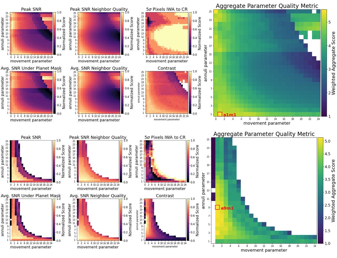
The pyKLIP-PE algorithm extracts four image quality metrics for injected (or real) companions. These are: (1) the peak pixel values of each planet in the SNR map (“peak SNR metric”), (2) the average SNR of all positive pixels within 0.5xFWHM radially and 5∘ azimuthally of each planet in the SNR map (“average SNR metric”), (3) the achieved contrast at the location of each planet, and (4) the number of false-positive (5) pixels between the IWA and the AO control radius. An additional two metrics, which we call “neighbor quality” metrics, are computed by smoothing the peak and average signal-to-noise metrics across pyKLIP’s movement and annuli parameters. These metrics are based on the anecdotal understanding prevalent in the community that the most robust KLIP detections are those where small variations in KLIP parameters do not substantially affect the recovered planetary SNR.
In this work, we choose a simple equally weighted sum of all six normalized metrics. We then average the sum of these normalized metrics across all false planets, thereby balancing recovery of signals throughout the region of interest. As a further measure to ensure robustness, we average the 5 and 20 KL mode aggregate parameter quality maps before selection of a final movement, annuli combination. As described in detail in Adams Redai et al. 2023, these particular KL modes were chosen based on the statistical distribution of optimal parameter choices for HD 142527 B recovery under a range of optimization scenarios.
Effectively, this methodology means that the algorithm attempts to select an annuli and movement combination that results in robust (according to all six metrics) extraction of injected planets throughout the region of interest for both low (=5) and moderate (=20) PSF model complexity. Once this combination of annuli and movement parameters is chosen, the final choice of “optimal” KL mode is made by maximizing the sum of all six metrics for that dataset averaged over all injected planets. Optimal annuli, movement, and numbasis (KL mode) parameters selected using this methodology are reported for each dataset in Table 5. Unless otherwise indicated, all post-processed images shown in this work have pyKLIP parameters selected via this methodology.
Figure 5 shows two examples of normalized parameter quality maps for all six image quality metrics averaged across all injected continuum planets and among 5 and 20 KL modes. The aggregate parameter quality map is shown in the large panel at right, and the optimal annuli and movement parameters are indicated. A complete description of how we arrived at this method, as well as detailed discussion of the features of these maps, can be found in Adams Redai et al. 2023.
| General Dataset Parameters | Data Quality Cut Parameters | KLIP Optimization Parameters | |||||||||||
| Object | Date | Ntotal | Bin | rsat | IWA | Cfakes | Cut | FWHM | Cut Classification | Annuli | Movement | KL Modes | |
| CS Cha | 5/15/15 | 143 | 2 | 7 | 0.05 | 30 | 7 | down and up inside 02 | 2 | 6 | 2 | 3 | |
| HD 100453 | 2/17/17 | 2947 | 1 | 3 | 4 | 0.01 | 10 | 4 | clustered, increasing | 5 | 5 | 3 | 10 |
| HD 100453 | 5/2/18 | 356 | 1 | 2 | 3 | 0.01 | 40 | 3 | clustered, increasing | 8 | 8 | 1 | 20 |
| HD 100453 | 5/2/18 | 563 | 1 | 4 | 4 | 0.01 | 30 | 3 | clustered, increasing | 7 | 13 | 1 | 20 |
| HD 100453 | 5/3/18 | 2831 | 1 | 4 | 4 | 0.01 | 70 | 3 | turnover at 007 | 7 | 19 | 1 | 20 |
| HD 100546 | 4/12/14 | 4939 | 1 | 8 | 8 | 0.01 | 10 | 5 | clustered, increasing | 3 | 13 | 1 | 10 |
| HD 100546 | 5/30/15 | 2459 | 1 | 2 | 4 | 0.05 | 50 | 4 | turnover at 012 | 5 | 25 | 2 | 5 |
| HD 141569 | 4/9/14 | 2402 | 1 | 5 | 5 | 0.01 | 70 | 5 | turnover at 015 | 4 | 1 | 1 | 5 |
| HD 141569 | 4/10/14 | 1364 | 1 | 2 | 6 | 0.01 | 50 | 6 | turnover at 015 | 3 | 2 | 4 | 1 |
| HD 141569 | 4/11/14 | 2340 | 1 | 4 | 4 | 0.01 | 10 | 4 | clustered, increasing | 5 | 4 | 5 | 20 |
| HD 141569 | 5/28/15 | 723 | 1 | 7 | 0.05 | 70 | 7 | decreasing | 2 | 2 | 4 | 2 | |
| HD 141569 | 5/29/15 | 404 | 1 | 9 | 9 | 0.01 | 0 | 4 | increasing | 4 | 1 | 5 | 5 |
| HD 142527 | 4/11/13 | 1961 | 1 | 3 | 0.01 | 10 | 3 | clustered, increasing | 8 | 14 | 1 | 20 | |
| HD 142527 | 4/8/14 | 1758 | 1 | 4 | 0.01 | 0 | 4 | clustered, increasing | 5 | 25 | 1 | 100 | |
| HD 142527 | 4/8/14 | 68 | 1 | 11 | 11 | 0.01 | 0 | 5 | increasing | 2 | 21 | 1 | 10 |
| HD 142527 | 5/15/15 | 2387 | 1 | 2 | 4 | 0.01 | 50 | 4 | clustered, increasing | 5 | 2 | 2 | 20 |
| HD 142527 | 5/16/15 | 1143 | 1 | 2 | 6 | 0.05 | 80 | 4 | turnover at 03 | 5 | 20 | 1 | 20 |
| HD 142527 | 5/18/15 | 159 | 1 | 6 | 6 | 0.01 | 0 | 4 | clustered, increasing | 4 | 2 | 7 | 5 |
| HD 142527 | 2/10/17 | 242 | 1 | 2 | 3 | 0.05 | 0 | 4 | increasing | 5 | 25 | 1 | 5 |
| HD 142527 | 4/27/18 | 580 | 1 | 3 | 3 | 0.05 | 0 | 3 | clustered, increasing | 8 | 22 | 1 | 10 |
| HD 169142 | 4/8/14 | 2796 | 1 | 4 | 0.01 | 80 | 4 | turnover at 0 | 5 | 1 | 1 | 20 | |
| HD 169142 | 4/9/14 | 178 | 1 | 6 | 6 | 0.01 | 50 | 5 | clustered, increasing | 3 | 20 | 1 | 4 |
| HD 169142 | 5/18/15 | 1731 | 1 | 3 | 5 | 0.01 | 20 | 5 | clustered, increasing | 4 | 6 | 2 | 20 |
| HD 169142 | 8/30/17 | 1658 | 1 | 2 | 4 | 0.05 | 70 | 4 | turnover at CR | 5 | 6 | 2 | 20 |
| LkCa 15 | 11/16/14 | 308 | 2 | 6 | 0.05 | 5 | 7 | clustered, increasing | 2 | 4 | 6 | 20 | |
| LkCa 15 | 11/18/16 | 252 | 2 | 7 | 0.05 | 10 | 11 | mostly increasing | 1 | 10 | 1 | 20 | |
| PDS 66 | 2/7/17 | 243 | 2 | 5 | 0.01 | 40 | 5 | clustered, increasing | 2 | 2 | 1 | 1 | |
| PDS 70 | 2/8/17 | 188 | 2 | 7 | 0.05 | 40 | 7 | down and up in inner 015 | 2 | 1 | 1 | 1 | |
| PDS 70 | 5/2/18 | 209 | 2 | 6 | 0.05 | 5 | 6 | clustered, increasing | 2 | 4 | 1 | 4 | |
| PDS 70 | 5/3/18 | 284 | 2 | 6 | 0.05 | 30 | 6 | down and up in inner 01 | 2 | 3 | 7 | 50 | |
| SAO 206462 | 4/12/14 | 3993 | 2 | 3 | 4 | 0.01 | 30 | 4 | down and up | 5 | 1 | 1 | 3 |
| SAO 206462 | 5/26/15 | 408 | 2 | 4 | 0.05 | 30 | 4 | clustered, increasing | 3 | 1 | 2 | 2 | |
| TW Hya | 4/8/14 | 1958 | 2 | 5 | 0.01 | 50 | 5 | turnover at 015 | 2 | 5 | 2 | 1 | |
| TW Hya | 2/7/17 | 452 | 2 | 2 | 6 | 0.01 | 0 | 6 | increasing | 2 | 6 | 6 | 50 |
| UX Tau A | 11/15/14 | 52 | 2 | 8 | 0.05 | 8 | 30 | clustered, increasing | 2 | 6 | 2 | 50 | |
| V1247 Ori | 11/15/14 | 893 | 2 | 4 | 0.01 | 50 | 4 | turnover at CR | 3 | 2 | 9 | 10 | |
| V1247 Ori | 12/11/15 | 878 | 2 | 5 | 0.01 | 60 | 5 | turnover at CR | 2 | 2 | 6 | 50 | |
| V4046 Sgr | 4/12/14 | 1414 | 2 | 2 | 5 | 0.01 | 50 | 5 | turnover at 015 | 2 | 21 | 2 | 20 |
| V4046 Sgr | 5/17/15 | 720 | 2 | 4 | 0.01 | 50 | 4 | down and up | 3 | 13 | 1 | 50 | |
IV Survey Analysis Methodologies
In this section, we provide explanations of various methods used to generate the final, optimized images and sensitivity limits for the GAPlanetS companion candidate search, results of which appear in Section V and VI. We also detail the tools used for candidate characterization, including the procedure for obtaining a final estimation of mass accretion rate.
KLIP-ADI images
are shown in Section V and Appendix B for all GAPlanetS targets. For those targets with known companions or companion candidates detected in GAPlanetS data, all epochs (including nondetection epochs) are shown in the main body of the text for completeness. As there are less robust 2-4 excess signals at a number of locations in most datasets, additional epochs for objects without recovered candidate companions are shown in Appendix B. Some of these signals may prove in the future to be protoplanets upon higher-contrast follow-up and/or additional epochs of observation.
Optimization strategies
One important consideration in extracting point-source signals from these data is whether to conduct analyses on post-processed images that have undergone conservative KLIP parameter optimization (on false planets injected into the continuum data, as described and shown in Section III.2), or to optimize on the known location of the companion(s) in H images. The relative merits of each of these strategies is discussed in detail in Adams Redai et al. 2023. In short, optimization on false planets injected into the continuum data is a robust method that is substantially less likely to yield false-positive detections. We apply it to all datasets to achieve a uniform analysis. However, there is necessarily a penalty in the final signal-to-noise ratio of recovered H companions by virtue of the optimizations being done on a different (albeit contemporaneous and close-in wavelength) dataset and averaged over planets located throughout the region of interest rather than at a particular PA and separation. In the case of very robust high-SNR recoveries, this penalty is of minimal concern as the companion is recovered using both strategies. However, in the case of detections at or near the detection threshold, this SNR penalty may result in nonrecovery of the companion under the continuum optimization method. In cases where the point-source nature of the companion is robustly established in the literature (HD 142527 B and PDS 70 b and c, all of which have been detected at continuum wavelengths in addition to H) and the companion is unrecovered under the standard survey optimization methodology, we report optimizations done directly on the H imagery at the companion location as well. We note that such direct optimization on the H images, though it is more likely to result in a recovery of planetary signal, risks overfitting and should be interpreted with caution. To mitigate this somewhat, we adopt a relatively conservative version of this direct optimization approach by averaging across several KL modes and image quality metrics (for difficult HD 142527 B recoveries) or across several known companions (for PDS 70).
ASDI images
All KLIP image panels (figures 7–14 and all figures in Appendix B) show H (left) and continuum (middle left) reductions, as well as two ASDI images. The first (middle right) image is a conservative reduction computed by scaling the pyKLIPed continuum image up by the median stellar H/continuum brightness ratio (as described in Section II.4). The second (right) ASDI reduction is computed by subtracting the two at 1:1 scale. The relative fidelity of the two types of SDI reduction is nuanced and is discussed in detail in Section II.4. To recap briefly here, scaling and subtracting by the H/continuum brightness ratio should effectively remove both scattered light and stellar residuals, where present. However, in the absence of such signals/residuals, the 1:1 scaled reduction is the more accurate indicator of H excess. We show both, as well as the pyKLIP-reduced H and continuum images in order to provide full context with which to judge the fidelity of any apparent signals.
Robustness of signals among H and SDI images
is an important concern in extracting accurate photometry and astrometry for GAPlanetS candidates. The highest-fidelity signals are present in both H and SDI images. While the SDI process helps to remove disk signal and stellar residuals, as well as the continuum contribution of objects like HD 142527 B, it can also induce false-positive signals into SDI imagery. This occurs when a negative speckle in the KLIP-processed continuum images is reversed during SDI subtraction, becoming positive. Negative continuum speckles with sufficient amplitude to mimic planetary signals are relatively uncommon, but are visible and appear point-source-like in several GAPlanetS datasets (=2). These spurious point-sources are marked with yellow “x” symbols in all SDI images where they are apparent.
Multiepoch combinations
(post-KLIP mean combinations) are utilized in cases where independent datasets were acquired for a given object within several days of one another. Although this technique of combining post-processed KLIPed images from multiple near-in-time epochs has been shown to yield detections in some cases where single epoch images do not reveal a high SNR source (Wagner et al. 2018a, e.g.;), we caution that accreting companions are also likely variable, so higher SNR detections will only result in cases where the object is accreting at a detectable rate in both epochs. Given the detectable level of H variability seen on night-to-night timescales in GAPlanetS objects (see Balmer et al. 2022), accretion rates derived from combined data should be interpreted with caution.
Contrast curves
Astrometry of detected companions
is computed via the Bayesian KLIP Astrometry (BKA) technique described in detail in Wang et al. 2016 and implemented via pyKLIP. In short, the technique creates a forward model by projecting one or more PSFs onto the KL basis set. This results in a post-processed PSF that replicates the complex shape of the planetary core and self-subtraction lobes unique to a given dataset, choice of KLIP parameters, and point-source location. This forward-modeled PSF is adjusted astrometrically and photometrically to produce quality-of-fit posterior distributions. BKA input can be either a single fixed PSF or a time-variable PSF cube. Given the demonstrated high degree of PSF variation in GAPlanetS data, we have opted for the latter. Our input PSF model is therefore a time series of normalized image stamps, one per image in the sequence. We report astrometric (and photometric) values for companions as the median of the BKA posterior distribution.
Contrasts of companion candidates
are also fit with BKA. In our case, we ensure that the PSF model (star or ghost image) has a fixed contrast by normalizing it and then multiplying by a fixed contrast that we know is reasonably close to that of the companion. Preprocessed images are also normalized (by dividing each image by the peak of a Moffat fit to the central star in the case of unsaturated data or the ghost multiplied by the established ghost-to-star scale factor in the case of saturated data) in preprocessing before injecting false planets and running KLIP. By normalizing the input images to a peak value of one and the input PSF to the “best guess” contrast, this ensures that the simulated point-source is modeled at a fixed contrast relative to the time-varying central PSF. After computation of the forward model, the post-processed PSF brightness is iterated upon during BKA analyses with a scale factor parameter that we multiply by the initial contrast guess to get the final best-fit contrast value for a companion.
Uncertainties on companion astrometry and photometry
are reported as the 67% credibility interval of the BKA posterior distributions for separation, position angle, and contrast. Uncertainty on absolute astrometric calibration of the instrument and the location of the central star in the images is incorporated into the error estimation for those quantities. However, the reported error bars for contrast encompass only the 67% credibility interval for the scale factor posterior and not any uncertainties in photometric calibration, which we propagate separately into accretion rate estimates, as described in detail in Section VI.
Detection strengths
are characterized further by utilizing the PlanetEvidence class (Golomb et al. 2019) within pyklip to conduct a Bayesian model comparison and make a more conservative SNR estimate for each companion detection. These values are reported in Table 5. PlanetEvidence uses the nested sampling implementation pyMultiNest (Buchner 2014; Feroz et al. 2009) to compare two models: , where the image contains only speckle noise, and , where the image contains a source at the position of the companion. PlanetEvidence returns marginal distributions of the parameters for the source and null cases, and calculates the SNR of the detection within the fitting region and the evidence values for and ( and ). The log-ratio of these evidence values, , enables us to quantify the confidence with which one model can be favored over the other. This framework provides a more robust estimate of the quality of the detection because it better captures asymmetric speckle noise, which can dominate at very close separations. Values for are considered “strong” evidence against the null hypothesis. We note that PlanetEvidence-extracted SNR and values are sensitive to the size of the BKA fitting region, and can vary by 10% based on this choice. We adopt a 15 pixel square fitting region for all forward model fits except in cases where nearby residual structure results in a clear under- or over-subtraction of the point-source candidate.
V Individual Object Results
This section outlines GAPlanetS results for each transitional disk in the sample and describes in basic terms the recovery (or lack thereof) of confirmed or candidate protoplanets. In each case, the data have been preprocessed as described in Section II, culled as described in Section III.1, post-processed with pyKLIP with parameters optimized for false planets injected into continuum images as described in Section III.2, and images and contrast curves generated following the methods described in Section IV.
The object-by-object results are aggregated in this section into previously reported GAPlanetS detections (Section V.1), new planet candidates (Section V.2), other objects for which known or candidate companions exist in the literature (Section V.3), and objects with no known or candidate companions (Section V.4). Survey-level analyses follow in Section VI. Literature predictions for the locations of companions and companion candidates are shown in all images, and these predictions are compiled in Table 4. In most cases, literature candidate companions are not detected in GAPlanetS imagery, and detection limits at their predicted locations are summarized in Section VI.2.
In cases where companions or companion candidates are successfully detected in H and/or continuum GAPlanetS imagery, best-fit astrometry and photometry, computed as described in section IV, is summarized in the text. Astrometric and photometric fit statistics and forward models follow in section VI.1.
| Object | Label | Epoch(s) | Sep | Sep Error | PA | PA Error | Source |
| (pix) | (pix) | (deg) | (deg) | ||||
| Previous GAPlanetS Detected Objects with Epoch-Specific Location Measurements/Predictions | |||||||
| HD 142527 | B | 04/11/2013 | 10.2 | 0.1 | 126.0 | 0.5 | Balmer et al. 2022 |
| HD 142527 | B | 04/08/2014 | 9.7 | 0.2 | 115.9 | 1.0 | Balmer et al. 2022 |
| HD 142527 | B | 05/15/2015 | 8.4 | 0.2 | 109.6 | 0.8 | Balmer et al. 2022 |
| HD 142527 | B | 05/16/2015 | 8.6 | 0.3 | 108.6 | 1.0 | Balmer et al. 2022 |
| HD 142527 | B | 05/18/2015 | 8.6 | 0.2 | 110.2 | 0.7 | Balmer et al. 2022 |
| HD 142527 | B | 02/10/2017 | 6.4 | 0.2 | 77.8 | 2.0 | Balmer et al. 2022 |
| HD 142527 | B | 04/27/2018 | 4.8 | 0.3 | 58.0 | 1.8 | Balmer et al. 2022 |
| PDS 70 | WiPb | 02/08/2017 | 23.3 | 0.2 | 149.7 | 0.3 | Wang et al. 2021b |
| PDS 70 | WiPc | 02/08/2017 | 28.1 | 0.1 | 283.8 | 0.2 | Wang et al. 2021b |
| PDS 70 | WiPb | 05/02/2018 | 22.6 | 0.1 | 146.8 | 0.3 | Wang et al. 2021b |
| PDS 70 | WiPc | 05/02/2018 | 27.7 | 0.1 | 281.2 | 0.1 | Wang et al. 2021b |
| PDS 70 | WiPb | 05/03/2018 | 22.6 | 0.1 | 146.7 | 0.3 | Wang et al. 2021b |
| PDS 70 | WiPc | 05/03/2018 | 27.7 | 0.1 | 281.2 | 0.1 | Wang et al. 2021b |
| LkCa 15 | S14b | 11/16/2014 | 11.7 | 1.0 | 256 | 3 | Sallum et al. 2015 |
| LkCa 15 | S14c | 11/16/2014 | 10.1 | 1.5 | 318 | 11 | Sallum et al. 2015 |
| LkCa 15 | S14d | 11/16/2014 | 10.9 | 8.8 | 14 | 30 | Sallum et al. 2015 |
| LkCa 15 | S16b | 11/18/2016 | 12.2 | 0.8 | 248 | 2 | Sallum et al. 2016 |
| LkCa 15 | S16c | 11/18/2016 | 10.9 | 0.5 | 301 | 2 | Sallum et al. 2016 |
| LkCa 15 | S16d | 11/18/2016 | 10.3 | 2.0 | 348 | 5 | Sallum et al. 2016 |
| Other Candidate Detections and Predictions from the Literature | |||||||
| PDS 70 | Z20d | Feb-July 2020 | 13.8 | NR | 310 | NR | Zhou et al. 2021 |
| HD 169142 | O07 | June 2007 | 14.6 | 2.5 | 250.0 | 5.0 | Okamoto et al. 2017 |
| HD 169142 | O12-13 | 2012-2013 | 42.8 | NR | 175.0 | NR | Osorio et al. 2014 |
| HD 169142 | R13 | June 2013 | 19.6 | 4.0 | 7.4 | 11.3 | Reggiani et al. 2014 |
| HD 169142 | B13 | July 2013 | 13.8 | 3.8 | 0.0 | 14.0 | Biller et al. 2014 |
| HD 169142 | B14 | April 2014 | 22.6 | NR | 33.0 | NR | Biller et al. 2014 |
| HD 169142 | G15-17A | 2015-2018 | 14.5 | 1.9 | 239.0 | 11.5 | Gratton et al. 2019 |
| HD 169142 | G15-18B | 2015-2018 | 23.8 | 1.0 | 17.0 | 8.0 | Gratton et al. 2019 |
| HD 169142 | G15-18C | 2015-2018 | 24.8 | 1.1 | 308.0 | 9.0 | Gratton et al. 2019 |
| HD 169142 | G15-18D | 2015-2018 | 39.9 | 0.9 | 39.0 | 5.0 | Gratton et al. 2019 |
| HD 169142 | B18 | July 15, 2018 | 13.3 | 4.4 | 55.5 | 4.0 | Bertrang et al. 2020 |
| HD 100546 | Q11 | May 2011 | 59.0 | 1.5 | 7.0 | 1.4 | Quanz et al. 2013 |
| HD 100546 | C15 | Jan 2015 | 16.5 | 1.1 | 150.9 | 2.0 | Currie et al. 2015 |
| HD 100546 | S15-16 | 2015-2016 | 57.2 | 0.9 | 11.5 | 1.1 | Sissa et al. 2018 |
| HD 100546 | F15-16 | 2015-2016 | 121.3 | NR | 10 | NR | Fedele et al. 2021 |
| SAO 206462 | C16 | March 2016 | 8.9 | 0.6 | 19.0 | 3.0 | Cugno et al. 2019 |
| SAO 206462 | C19 | July 13, 2019 | 53.6 | 0.2 | 212.4 | 0.7 | Casassus et al. 2021 |
| TW Hya | I16 | Dec 2016 | 105.7 | 8.5 | 242.5 | 2.1 | Ilee et al. 2022 |
| TW Hya | T17 | May 2017 | 108.9 | 0.1 | 237 | 1 | Tsukagoshi et al. 2019 |
| TW Hya | H19 | March 15, 2019 | 20.1 | 1.3 | 190 | 1 | Huélamo et al. 2022 |
| CS Cha | G17 | Feb-Jun 2017 | 165.6 | 0.6 | 261.4 | 0.2 | Ginski et al. 2018 |
| HD 100453 | W17 | Feb 17, 2017 | 132.83 | 0.40 | 132.32 | 0.18 | Wagner et al. 2018b |
| HD 100453 | G19 | April 7, 2019 | 135.1 | 4.0 | 132.7 | 0.8 | Gonzalez et al. 2020 |
| V1247Ori | W12-13 | 2012-2013 | 5.2 | 0.8 | 305.5 | 5.5 | Willson et al. 2019 |
V.1 Objects with Previously Reported GAPlanetS Detections
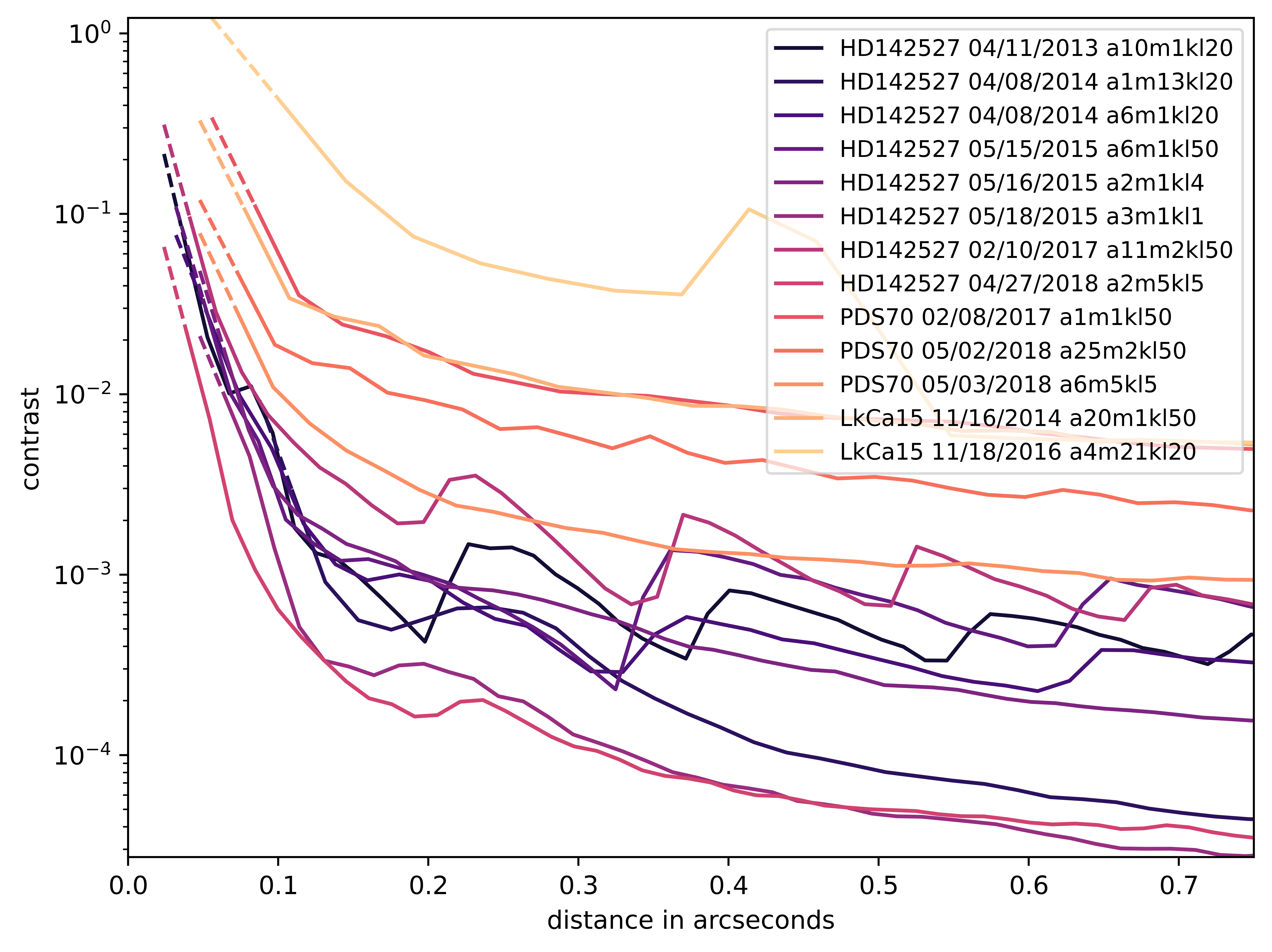
GAPlanetS data have already revealed three low-mass accreting companions and companion candidates: HD 142527 B, LkCa 15 b, and PDS 70 b, reported in Close et al. 2013; Sallum et al. 2015; Wagner et al. 2018a, respectively. In this section, we present uniform reprocessings of the data for each of these targets under the GAPlanetS campaign framework, as well as contrast curves for all epochs (See Figure 6).


V.1.1 HD 142527
The HD 142527 GAPlanetS datasets served as an excellent resource for optimizing and testing registration, centering, flat-fielding, dataset selection, and parameter optimization techniques for the GAPlanetS pipeline. The presence of the robust, high-SNR companion HD 142527 B allowed us to gauge the relative efficacy of various algorithmic choices on the recovery of the real companion at tight separation.
GAPlanetS data were collected for HD 142527 in 2013, 2014, 2015, 2017, and 2018. We include continuum-optimized imaging and contrast results for all epochs in Figure 7, and H optimized reductions for the most difficult detections in Figure 8.
Photometric and astrometric monitoring and orbit fitting of HD 142527 B are the subject of a companion paper (Balmer et al. 2022) and are not discussed in detail here. Importantly, Balmer et al. 2022 refined the orbit of the companion and demonstrated that it is significantly misaligned () with respect to both the inner and outer disk components. We touch briefly on consistency between our astrometric and photometric fits and those of Balmer et al. 2022 in Section VI.
Figure 7 demonstrates that HD 142527 B is easily recovered in H, continuum, and SDI imagery in datasets from 2013 (SNR=10.5/7.5/5.6 for H, continuum, and 1:1 scaled SDI imagery, respectively), 2014 (SNR=6.8/3.6/4.6), May 15 2015 (SNR=9.0/3.7/8.0), May 16, 2015 (SNR=5.7/3.5/4.1) and May 18 2015 (SNR=7.0/5.2/4.5) following the bulk survey strategy of optimizing on false planets injected into continuum images.
The 2017 and 2018 HD 142527 datasets are substantially more difficult detections than the 2013–2015 epochs, as the predicted separation of HD 142527 B is much tighter (005, 6pix). We attempted both continuum-optimized and H companion-optimized reductions of these datasets. The companion is recovered in 2018 H data at an SNR of 3.9 in the direct H optimized reduction, but is not recovered in 2017 under either optimization method. The reason for this is readily visible in the contrast curves of Figure 6, which reveal that even the most highly optimized pyKLIP reduction of the 2017 dataset boasts nearly an order-of-magnitude poorer contrast at the location of the companion than the next-lowest-quality dataset. This is likely a result of both the extremely tight separation of the companion at this epoch and the small amount of on-sky rotation obtained (16.1∘). More detail on the nature of the 2018 recovery is provided in Balmer et al. 2022.
The source of the 140au (Avenhaus et al. 2014) gap in HD 142527 has been debated, in particular whether the binary companion HD 142527 B can be solely responsible for carving the wide central cavity (Fukagawa et al. 2006; Biller et al. 2012; Casassus et al. 2015; Price et al. 2018). In 2014 and 2015, we conducted deep imaging of the system to search for outer companions in the wide disk gap, allowing the detector to saturate out to near or beyond the companion’s location. No additional candidates were found in either epoch.


V.1.2 PDS 70
We observed PDS 70 as part of the GAPlanetS campaign in 2017 and 2018. H emission from PDS 70 b from data taken in 2018 on two consecutive nights was reported in Wagner et al. 2018a, establishing PDS 70 b as an accreting protoplanet. Frame selection, highpass filter, and KLIP parameters were tuned aggressively to allow for robust recovery of the companion at in the combination of post-processed SDI imagery from the two 2018 nights. H line emission was subsequently resolved in both PDS 70 b and c by Haffert et al. 2019 with the Very Large Telescope (VLT) Multi Unit Spectroscopic Explorer (MUSE) instrument, and in ultraviolet accretion continuum emission with the Hubble Space Telescope (HST) by Zhou et al. 2021, lending additional credence to the original detection.
Figure 9 shows the continuum false planet optimized reductions for all three PDS 70 epochs, as well as the combination of the two 2018 nights. Overplotted on these images are the predicted locations of the two known companions at the epoch of observation, derived from the orbital fits of Wang et al. 2021b. Contrast curves for all PDS 70 epochs are shown in Figure 6. By optimizing on false continuum planets injected at a range of separations between the IWA and control radius of each dataset, the GAPlanetS reduction framework is intentionally conservative. Both PDS 70 planets lie considerably outside the control radius; thus, the lack of recovery under the standard pipeline is unsurprising. While neither companions is robustly recovered, a 3 excess signal appears within 1 FWHM of the predicted location of PDS 70 c in both H and ASDI images for the 2017 epoch and in ASDI images for the 2018 May 2 epoch.
Both known planets are recovered with more targeted optimization (see Figure 10). As the PDS 70 b and c companions exist at known locations and their bona fide planetary nature is well established, we follow the same procedure as for the more difficult HD 142527 B recoveries in order to recover their signals where possible. Namely, we optimize directly on the average SNR metric at the known planet location(s) in the H images. We choose to average this SNR metric across both known planet locations in order to achieve a relatively conservative approach to this direct H optimization.
We note that this optimization is done using the H images only and not SDI images. Because of the prevalence of false point-sources induced during subtraction of KLIP-ed continuum imagery, we believe that optimizing on the H images is a more robust approach.
Reductions tuned to maximize the average SNR metric across both planets in 20 KL mode H post-processed imagery are shown in Figure 10, with their optimized KLIP parameters given in the labels on the left-hand side of each subpanel. The companions are only readily visible in SDI imagery using this methodology, but both are marginally recovered. A signal consistent with PDS 70 c is present in all three SDI epochs, with classically computed SNRs of 3.8/2.6/2.9 and 3.1/3.0/3.4 in 1:1 scaled and conservatively scaled SDI images, respectively. It is also marginally recovered in H at an SNR of 3.7 in the 2017 epoch. PDS 70 b is recovered only in the 2018 May 3 epoch at an SNR of 3.3 in 1:1 scaled SDI imagery and 2.8 in conservatively scaled SDI imagery.
We extract detailed astrometry and photometry only from the 2017 H detection of PDS 70 c, as forward model fitting of SDI imagery is more complex and beyond the scope of this work. We note, however, that the positions of the marginal detections of PDS 70 b and PDS 70 c in 2018 SDI imagery are entirely consistent with their whereistheplanet predicted orbital positions (see Figure 10, which incorporates the astrometry of Wagner et al. 2018a and other works.
Our 2017 detection of PDS 70 c extends the time baseline of its astrometry by 9 months. The companion is detected at a separation of 246.94.4mas and a PA of 284.20.6∘. This is inconsistent at the 5 level with the whereistheplanet (Wang et al. 2021a) prediction for the separation of the planet at this epoch (223.20.9mas), though the PA prediction (283.80.2∘) is consistent. Our best-fit photometry suggests a mag of 5.50.2 relative to the stellar continuum, brighter by nearly 2 magnitudes than the 7.70.2 reported from VLT MUSE observations taken a year later by Haffert et al. 2019. Possible sources of these discrepancies are discussed in Section VI.1.

V.1.3 LkCa 15 b
LkCa 15 was observed three times as part of the GAPlanetS campaign, in 2014, 2015, and 2016. The 2014 epoch is the original H discovery epoch for LkCa 15 b, as well as the highest-contrast epoch (see Figure 11). The 2015 data were of very poor quality and were discarded before KLIP optimization due to a failure to recover injected planets at a contrast of 10-1. The 2016 dataset is of intermediate quality, though substantially poorer in contrast than the 2014 epoch, and the companion candidate is not recovered (see Figure 6).
The existence of multiple protoplanet candidates in close proximity to the inner disk rim of LkCa 15 has been the source of some controversy. Recent work by Currie et al. 2019 resolved the inner disk component previously imaged by Thalmann et al. 2016 in polarized intensity, this time in NIR total intensity light with SCExAO on Subaru and in the thermal infrared with Keck/NIRC2. The authors interpret the smooth resolved inner disk rim as inconsistent with the existence of multiple protoplanets at similar separation; however, their results cannot explain observed orbital motion in the sparse aperture masking detections (Sallum et al. 2016), nor is an inner disk artifact consistent with the presence of H excess emission in the companion.
Mendigutía et al. 2018 attempted spectroastrometric detection of H emission from the LkCa 15 b planet candidate and reported symmetric extended H emission. However, their observation relied on long-slit spectroscopy that does not appear to have been well aligned with the predicted position of LkCa 15 b at that epoch
Even if the companion was in the slit, the reported detection threshold was a contrast of 5.5 mag at H, close enough to the mag of 5.20.3 reported in Sallum et al. 2015 that even a small decrease in luminosity relative to the original 2014 November H detection epoch (as might be expected if accretion onto the companion is stochastic) would render the planet undetectable.
As the nature of the point-source candidates in the LkCa 15 disk has been debated and their proximity to the resolved inner disk rim firmly established, we adopt the most conservative approach in this work – optimizing on false continuum planets only. We also overplot an ellipse in Figure 11 at the edge of the imaged inner disk rim. While the LkCa 15 “c” and “d” candidates are coincident with the inner disk rim, the “b” candidate lies significantly inside of it and is less likely to be a scattered light artifact, though we note that disk signal at similar separation to planet candidates can influence extracted KL modes (Lawson et al. 2022) and further vetting of this candidate is warranted.
Because of the tight separations of the companion candidates, the comparatively large PSF (FWHM6pixels, 50mas), and the limited space available inside of the AO control radius for bin 2 data (=15 pixels), we injected only one false planet inside the control radius (at a separation of 12 pixels/010 and a PA of 0∘) to optimize these data.
Using our conservative optimization methodology, we recover the 2014 H excess signal first reported in Sallum et al. 2015 with a classically computed SNR of 5.0 in the H images, 4.9 in the 1:1 scaled H – continuum SDI reduction, and 2.9 in the conservatively scaled SDI reduction.
Best-fit BKA astrometry from the 2014 H epoch produces strong evidence (=18) for a point-source with a separation of 69.76.1 mas, a PA of 242.62.7∘ and a mag of 3.10.3. This is inconsistent at the 1–2 level with the astrometry and photometry derived from the same data in Sallum et al. 2015, which placed the planet at a slightly wider separation (938mas), higher PA (2563∘), and 1 magnitude fainter (Mag=5.20.3). This discrepancy is discussed in greater detail in Section VI.1.
While we recover a clear H signal in the 2014 epoch at the location of the previously reported LkCa 15 “b” planet candidate that is well fit by a point-source forward model, its nature remains ambiguous. The “b” candidate lies inside of the known scattered light inner disk rim, suggesting that it is not part of that structure. Although there is no apparent, comparable, point-source in the continuum images, scaling them up by the stellar H-to-continuum ratio and subtracting it from H suppresses the signal heavily, meaning that it cannot be ruled out as a scattered light source. At the same time, a compact scattered light structure located inside the disk cavity would itself be a notable result.
The optimized 2016 SDI reductions appear to show a low-SNR (2.5) arc of excess emission to the west of the star consistent with the known inner disk rim. The predicted location of LkCa 15 “b” lies inside of this rim, but it is not recovered. The contrast of these data are a factor of 5 or more worse than the 2014 epoch at all separations, making the lack of recovery of the candidate unsurprising. The high pyKLIP movement value converged upon by the continuum false planet optimization equates to a small reference library for PSF subtraction with a large degree of rotation between reference and target images. High rotational mask reductions are often used to resolve disk structures in ADI imagery, and this is likely the reason why the apparent disk rim is seen in 2016 but not 2014. Its appearance in SDI imagery is, however, surprising and could suggest an additional H emission source (i.e. the LkCa 15 b protoplanet) located to the west of the star, adding to the light being scattered by dust grains at this location.
There is also a 3 excess signal in the 2016 images at the predicted location of the “d” protoplanet candidate; however, there is a comparable signal to the south opposite this feature, which is suggestive of a wavefront error (phase) induced speckle.

In summary, we reproduce here, with a systematic and robust pipeline designed to minimize false positives, the original LkCa 15 “b” H detection reported in Sallum et al. 2015. We do not, however, recover the LkCa 15 “c” or “d” protoplanetary candidates, though this does not rule them out as protoplanets, as our achieved contrasts are modest at best.
V.2 Objects with New Protoplanet Candidates
V.2.1 CS Cha
One epoch of GAPlanetS data was obtained for the CS Cha AaAb spectroscopic binary (Kurtovic et al. 2022, unresolved, sep44mas;) in 2015. Although we do not see evidence of the wide polarized companion CS Cha B in post-processed images of this epoch (see Section V.3), we do find tentative evidence of a much more tightly separated point-source candidate with a classically computed SNR of 6.6 at H (PlanetEvidence SNR=4.3) located at a separation of 68mas and a PA of 76∘, as seen in Figure 13.
The observed separation of this candidate is roughly twice the value of the spectroscopic binary CS Cha A’s maximum predicted projected separation, suggesting that the imaged companion is not the other member of the binary. This detection places the candidate companion firmly within the disk’s sub-mm continuum (Francis & van der Marel 2020, 210mas;) and scattered light (Ginski et al. 2018, 92.5 - 337 mas;) cavities and interior to the probable inner edge of the gas cavity (Kurtovic et al. 2022, CO temperature peak at 128mas;). Simulations in Kurtovic et al. 2022 predict a Saturn-mass planet near the inner edge of the gas cavity, roughly consistent with the separation of the detected candidate. We note that their mass estimate is dependent on a viscosity assumption, and the presence of H emission may be suggestive of a more massive companion.
Its moderate contrast of 0.05 (3.2mag) relative to the (spectroscopic binary) primary suggests that the CS Cha “c” candidate may be massive or accreting at a very high rate. When corrected to a contrast relative to the stellar continuum (rather than the actively accreting primary), the contrast is even more moderate – 2.3mag. However, lack of detection in continuum imagery is more suggestive of a planetary nature. Due to these ambiguities and the lack of a second epoch, we refer to this detection as a protoplanet “candidate” throughout the remainder of this work.

V.3 Objects with Known Companions or Companion Candidates in the Literature
Six of the remaining transitional disks in the GAPlanetS sample have previous reports of planetary, brown dwarf, or stellar-mass companions from NIR high-contrast imagery, a sub-mm point-source interpreted as evidence of a circumsecondary disk, or a so-called ALMA “velocity-kink” indicative of possible inflow onto an embedded planet (Rabago & Zhu 2021, e.g.,). In each case, the reported location of the planet candidate(s) at the literature detection epoch is given in Table 4 and shown in all KLIPed images of the system. True companions will in most cases have undergone some small amount of orbital motion since this original detection epoch.
Three of the companions - HD 100546, HD 169142, and SAO 206462 - have previously reported planet candidates at low to moderate separation () from the central star. H, continuum, and ASDI images for all epochs of HD 169142 are shown in Figure 14 in order to demonstrate the difficulty of assessing protoplanet candidates in highly morphologically complex systems, while the other two objects’ reductions are shown in Appendix B. The contrast curves for all HD 100546, HD 169142, and SAO 206462 epochs are shown in Figure 12.
The remaining three objects - TW Hya, HD 100453, and CS Cha - have more distant (05) known or candidate companions, of which only HD 100453 B is recovered in GAPlanetS imagery. PyKLIP ASDI reductions for the highest-contrast epochs of these objects are shown in Figure 16. Optimized imagery of the inner regions of these three systems is shown in Appendix B. Contrast curves for all TW Hya, HD 100453, and CS Cha epochs are given in Figure 15.

V.3.1 HD 169142
GAPlanetS data of HD 169142 were collected on four nights - two consecutive nights in 2014, one night in 2015, and one night in 2017. All four epochs are shown in Figure 14. The data do not show a consistent excess at or near the location of any of the planet candidates across epochs; however, there are marginal signals consistent with H excess near the location of several candidates in single epochs. These signals do not rise to the level of candidates in our analysis because they are neither consistent across epochs nor have sufficiently high SNR. However, some may later prove to be true planetary signals in light of future observations at higher contrast.
We include all epochs of HD 169142 in the main body of the text as a demonstration of the difficulty of candidate identification in morphologically complex systems under variable conditions (and, potentially, intrinsic variability in protoplanet candidates’ H emission). For example, one of the more apparently compelling candidates in the images is a 3.5 point-source just outside the control radius near the Gratton et al. 2019 “D” candidate in the 2014 April 9 epoch (marked with a yellow circle in Figure 14). The lack of similar signal in the higher-contrast 2014 April 8 epoch just 1 day earlier, as well as its proximity to the AO control radius (immediately outside of which a bright ring of variable signal induced by the wavefront control loop appears in raw images), means that it does not rise to the level of a candidate in our analysis. Another 4 excess source appears to the northwest of the star in the 2017 August 30 epoch at similar separation as the Reggiani et al. 2014 and Biller et al. 2014 candidates (also indicated with a yellow circle in Figure 14). The 3 year time baseline between the original candidate identification epochs and this observation may allow for this degree of orbital motion; however, there is not a compelling excess at the same location in the H imagery, and similarly strong excess is not seen near this location in the other epochs, so this candidate is also marginal. We conclude that it and the other candidates at similar separation are most likely scattered light features from a clumpy inner disk ring at this separation, consistent with their lack of recovery in SDI imagery.
V.3.2 HD 100546
The GAPlanetS data for HD 100546 were analyzed in detail in Follette et al. 2017 and Rameau et al. 2017; however, we have taken advantage of improvements to the GAPlanetS pipeline since initial publication and reprocessed the data, allowing us to place more stringent limits on the H luminosity of the HD 100546 “b” and “c” planet candidates, as given in Table 6. No H excess signals were seen in the vicinity of either candidate in either GAPlanetS epoch (see Appendix B, Figure 20).
V.3.3 SAO 206462
GAPlanetS data were collected for SAO 206462 (HD 135344 B) in 2014 and 2015. No H excess signals were detected at or near the location of the Cugno et al. 2019 or Casassus et al. 2021 candidates in either epoch, and the best limit on the contrast at the location of these candidates is provided in Table 6. Images of both SAO 206462 epochs are shown in Appendix B, Figure 21.

V.3.4 TW Hya
GAPlanetS data of TW Hya were collected in 2014 and 2017. The highest-contrast (2014) ASDI epoch is shown in a wide-angle view in Figure 16, together with a zoomed-in view of the region surrounding the location of the candidate previously reported by Tsukagoshi et al. 2019 and Ilee et al. 2022. We note that TW Hya is accreting at an enormously high rate compared to the other objects in the sample, and the primary star is 6-8 times brighter at H than at the continuum in both epochs. This makes the difference between the 1:1 scaled SDI and the conservatively scaled SDI images striking and is an extreme example of the possible impact of incompletely removed stellar residuals on 1:1 scaled SDI images. At the same time, it is a clear demonstration of the power of measuring the stellar H/continuum ratio and scaling continuum imagery by it prior to SDI subtraction, as the residuals are very effectively removed in the conservatively scaled reduction shown in Figure 22. We do not find any evidence of H excess signals at the locations of the Tsukagoshi et al. 2019 or Huélamo et al. 2022 point-source candidates, nor elsewhere in the disk; however, both epochs are shown in Appendix B, Figure 22.

V.3.5 HD 100453
GAPlanetS data were collected for HD 100453 on one night in 2017 and two nights in 2018. The outer M dwarf companion HD 100453 B and a previously known background star at similar separation to the northeast are easily resolved, as seen in Figure 16. No additional point-source candidates are apparent in the imagery, including in the combination of the two 2018 datasets. A gallery of all HD 100453 epochs is shown in Appendix B, Figure 23.
HD 100453 B is a wide M star companion, robustly recovered in both H and continuum imagery in all GAPlanetS epochs, though it is saturated in all but the 2018 May 2 short exposure dataset. For this reason, we extract astrometry and photometry from the companion only at this epoch, and these values are given in Table 5. As the M dwarf companion is well characterized (Collins et al. 2009; Wagner et al. 2018b), we do not examine it in detail in this work.
HD 100453 B exhibits H excess, a clear indication of ongoing accretion, and an estimate for its accretion rate is given in Table 5. In contrast, the known background star to the northeast of the primary star is fully removed via ASDI except in the case of the deepest dataset, when some excess remains because the background star is saturated (see Appendix B, Figure 23).
V.4 Objects without Companion Candidates in the Literature
There are a number of GAPlanetS targets for which there are no previous reports of planet candidates at detectable separations (though there is a report of a very close companion to V1247 Ori, indicated in the images but under the inner mask), and there are no specific morphology-based predictions for protoplanet locations. These systems are HD 141569, PDS 66, UX Tau A, V1247 Ori, and V4046 Sgr. No compelling point-sources are detected in any of the epochs for these objects, though KLIP-ADI and ASDI images are shown for all epochs in Appendix B. Contrast curves for all epochs are given in Figure 17.

VI Survey Results

VI.1 Overview of Companion and Companion Candidate Photometry and Astrometry
In this section, we summarize our recovery of each of the five GAPlanetS companions and companion candidates. In all cases where the candidate recovery is sufficiently robust in H and/or continuum imagery, we extract astrometry and photometry using BKA as described in Section V and report the best-fit values in Table 5.
Figure 18 shows Bayesian KLIP astrometry models for all GAPlanetS point-source detections except for HD 142527 B, whose BKA fits we recompute under the unified GAPlanetS framework and report in Table 5, but which are similar to those described in detail in Balmer et al. 2022. Each image panel shows a stamp of the final optimized post-processed image, the corresponding best-fit forward model, and the residuals.
Our BKA fits returned “strong” evidence ratios for all five companions/candidates reported in Section VI. For PDS 70 c, LkCa 15 “b”, and CS Cha “c”, no point-source is recovered in the continuum, lending credence to the assertion of a planetary nature. HD 142527 B and HD 100453 B are recovered robustly in both H and continuum imagery, consistent with their nature as stellar companions. In both cases, planet-to-star contrast is more moderate at H than in the continuum for all epochs, suggestive of active accretion.
Compared to past observations, we find:
- •
HD 142527 B’s astrometry is entirely consistent with the observed position of the companion at similar epochs from other facilities, as discussed in detail in Balmer et al. 2022. We consider this excellent validation of our instrumental astrometric solution for VisAO.
- •
Although we have conducted HD 142527 reductions under a more conservative KLIP optimization framework, all astrometry is consistent with Balmer et al. 2022 to within error bars except for two of the three continuum epochs where the companion is recovered at SNR3 (2014 April 8 and 2015 May 15 astrometry disagrees with Balmer et al. 2022 at the 2 level). This suggests that BKA fitting is relatively robust to the choice of KLIP parameters, except in cases where SNR is very low.
- •
Measurement of the HD 142527 B companion’s continuum mag is consistent epoch-to-epoch to within error bars. It is also consistent with the continuum mag measured by SPHERE ZIMPOL (Cugno et al. 2019). This suggests that our photometric extractions for GAPlanetS data are broadly consistent with other HCI instruments.
- •
Measurement of HD 142527 B’s H mag is lower than the continuum mag at all epochs, with an average brightness increase of 0.9 mag over the continuum, suggestive of ongoing accretion. Our measurements are consistent with the observed H mag of Cugno et al. 2019 and with one another to within error bars. This is in conflict with the tentative evidence for accretion variability reported in Balmer et al. 2022, likely as a result of improved photometric extraction procedures described in detail in Section VI.2.
- •
PDS 70 c is detected at the same PA as predicted by whereistheplanet in 2017, but at a significantly (5) wider separation. As our astrometric solution has been extensively validated with astrometry of Trapezium cluster members and HD 142527 B, this offset is likely accurate, and the orbital properties of PDS 70 c should be updated.
- •
PDS 70 c’s best-fit H contrast translates to it being nearly 2 mag brighter relative to the host star in the 2017 epoch than the estimate of Haffert et al. 2019. Accretion rate variability for young stars is estimated to be on the order of 0.5 dex (Hartmann et al. 2016), a factor of 2 smaller than the magnitude differential between our observations and Haffert et al. 2019.
- •
LkCa 15 “b”’s astrometry and photometry is marginally (1–2) inconsistent with the values reported for the same dataset in Sallum et al. 2015, appearing at a tighter separation and lower PA. Improvements in the centering algorithm, VisAO astrometric solution, and post-processing techniques likely contribute to the observed astrometric offset of LkCa 15 “b” relative to previous estimates, as does the smaller IWA.
While our characterization of HD 142527 B is consistent with existing literature, for PDS 70 c and LkCa 15 “b”, our measurements of astrometry and photometry present inconsistencies with literature values. There are several possible reasons for this. Perhaps the most likely is that the extracted photometry and astrometry of companions, like many other qualities of post-processed images, are dependent on the choice of pre- (e.g., data quality cut, highpass filter value) and post- (e.g., IWA, annuli, and movement) processing parameters. Based on comparison of our BKA fits of HD 142527 B with those of Balmer et al. 2022 for the same datasets but with different pre- and post-processing choices, we believe that extracted astrometry of high-SNR (SNR3) sources is relatively robust to algorithmic parameters. Photometry, however, appears to be somewhat more sensitive to choices such as the BKA fitting area, especially as they effect the structure of the residuals, to which the photometry is very sensitive11 1 At the same time, we note that extraction of PDS 70 c astrometry and photometry in both continuum false planet optimized extractions (annuli=1, movement=1, numbasis=50) and direct H optimized extractions (annuli=17, movement=4, numbasis=20) is consistent within error bars despite extreme variation in KLIP parameters.. Importantly, uncertainty of this nature is not captured in our error estimates.
Absolute and relative photometric calibration of post-processed high-contrast images is also notoriously difficult. Though we have validated our photometric extractions relative to published photometry of HD 142527 B, and attempted to rigorously quantify photometric uncertainties, systematic errors remain possible.
VI.2 Determination of Accretion Rates and Limits
BKA-derived photometric contrasts for detected companions and final post-processed contrast limits for nondetected companion candidates from the literature are translated to accretion rates following the procedure described in this section. They appear with uncertainties in Tables 5 and 6.
VI.2.1 Computation of H Line Luminosities
In previous work (Close et al. 2014; Sallum et al. 2015; Wagner et al. 2015b; Follette et al. 2017; Rameau et al. 2017, e.g.,), H line luminosities () and limits on this quantity have been computed following the equation:
| (1) |
where is the distance in centimeters, is the instrumental zero-point of the H filter (Males 2013, erg cm2 sec-1 m-1 as determined by), is the width of the H narrowband filter (), is the star’s extinction corrected continuum magnitude in the H bandpass, and is the difference between the star and companion brightness at H in magnitude units (computed as -2.5log10(contrast)).
As the stellar continuum magnitude at H utilized in Equation 1 is not known, we use the apparent magnitude at the Sloan Digital Sky Survey (SDSS) ’ band as a proxy. We note that the ’ band is both centered near H (making the effect of any continuum slope across the bandpass minimal) and 25 times wider than the narrowband H filter width (making the contribution of any stellar H emission small compared to the overall ’ band flux). To achieve uniformity in the ’ band apparent magnitude estimates for our targets, we convert Gaia DR3 , and photometry (Gaia Collaboration et al. 2022a) to SDSS ’ magnitudes following the best-fit conversions of Alam et al. 2015. We note that these values are consistent with the values of the Gaia Synthetic Photometry Catalog 22 2 https://doi.org/10.17876/gaia/dr.3/64 of (Gaia Collaboration et al. 2022b, GPSC;) to within 0.1 mag for all eight GAPlanetS targets that are also in the GPSC.
’-band photometry is subject to nonnegligible extinction in nearby star forming regions, and this effect should be compensated for in estimating “true” ’-band apparent magnitudes for young stars. We estimate line-of-sight extinction to each GAPlanetS target by computing (BP-RP)=(BP-RP)obs-(BP-RP)0, where (BP-RP)obs is the observed Gaia BP-RP color of each system, and (BP-RP)0 is the intrinsic color derived from an update to (Pecaut & Mamajek 2013)33 3 Available at https://www.pas.rochester.edu/~emamajek/EEM_dwarf_UBVIJHK_colors_Teff.txt for a pre-main-sequence star of the same spectral type, assuming the spectral types reported in Table 1. (BP-RP) values have been shown to closely approximate literature values (Andrae et al. 2018, within 0.2mag;); therefore, we convert (BP-RP) to an ’-band extinction following standard Milky Way extinction laws (, ). We list our estimates, which are subtracted from the derived ’ band apparent magnitudes to compute a non-extincted ‘ magnitude estimate, in Table 1. We note that this estimate is based on stellar photometry alone, and that additional extinction toward companion candidates as a result of intervening circumstellar material is possible.
In this work, we also implement two minor corrections to the calculation described in Equation 1 for estimating LHα. First, because the central stars of our targets are themselves still actively accreting, the measured narrowband between the companion and the star is not really a mag relative to the stellar continuum, which would be required to compute an H luminosity. To make it so, we multiply the measured contrast () by the stellar H-to-continuum scale factor (, determined with aperture photometry as described in Section II.3 and reported in Table 2) to compute the companion’s H brightness ratio relative to the stellar continuum(). This value is reported in Tables 5 and 6 as mag. Due to the scale factor correction, it is not a direct magnitude conversion of the observed star-to-companion contrast, but rather a best estimate of the H excess unique to the companion.
LHα is also, properly, a line luminosity, meaning the companion’s continuum luminosity should be removed from the estimated H luminosity before using the derived value as a line luminosity. In the case where we detect continuum emission from the companion (HD 142527 B and HD 100453 B), this is easily done by substituting Cont for into equation 1 and subtracting the resulting continuum luminosity. In the case where an object is not detected at continuum wavelengths (PDS 70 c, LkCa 15 “b”, and CS Cha “c”), the contribution of the object photosphere to the H luminosity is unknown. However, we note that the predicted absolute continuum ’-band magnitude of even a very massive, very young planet is extremely faint (Baraffe et al. 2015, ’=14 for a 10 planet at 1 Myr;) compared to the H absolute magnitudes that we estimate for our planetary companions and companion candidates (MHα of 7.3, 8.8, and 12.3 for CS Cha “c”, LkCa 15 “b”, and PDS 70 c, respectively). It is thus reasonable to assume that any continuum contribution to the observed H luminosity for lower-mass companions is negligible.
In practice, these corrections and approximations make the equation used to compute H line luminosity:
| (2) |
where m is the stellar ’-band apparent magnitude, A is the estimated ’-band extinction, C is the observed H contrast of the companion, S is the stellar H-to-Continuum scale factor, and Lcont is the continuum contribution to the H luminosity (used only in the case of a continuum detection of the companion, otherwise assumed negligible).
As BKA does not natively propagate absolute photometric uncertainties, we compute our own uncertainty estimates for the final companion mag by propagating the uncertainties on a number of individual quantities into magnitude space. These uncertainties are: the 67% credibility interval on the best fit scale factor (the “alpha” value) from the BKA MCMC, uncertainty in the stellar H-to-continuum scale factor (estimated as the standard deviation in the scale factors of individual images in each observing sequence), and uncertainty in the stellar peak used to normalize imagery prior to BKA (estimated as the median photon noise of the best-fit stellar (unsaturated) or ghost (saturated) photometry). We also include uncertainty in the ghost-to-star scale factor in the case of saturated data, a value derived from the standard deviation of the residuals to the linear fit between ghost and stellar Moffat fit peak values in all unsaturated GAPlanetS datasets (23050 at H, 24550 at the Continuum).
Uncertainty on the final H luminosities encompasses uncertainty on mag, as well as uncertainties in the following quantities: the stellar ’-band apparent magnitude (assumed to be 0.1 based on the average discrepancy between our estimates and the GPSC), the ’-band extinction (estimated at 0.2 based on the range of estimates for AR of these objects in the literature), distance (derived from parallax uncertainty in the Gaia catalog), instrumental zero-point (estimated conservatively at 10%), and the companion’s continuum brightness (where detected, estimated following the same procedure as H photometric uncertainty).
VI.2.2 Estimation of Accretion Luminosities and Rates
Accretion luminosities are derived from H line luminosities following the equation:
| (3) |
where the coefficients and represent an empirically or model-derived scaling law between and accretion luminosity. The value of these scaling coefficients is particularly poorly constrained in the substellar regime. We report accretion rates for detected protoplanetary candidates and accretion rate limits for undetected literature companion candidates following both the Aoyama et al. 2021 (, , with scatter of 0.3 dex) and Alcalá et al. 2017 (, , with scatter of 0.5-0.7 dex) scaling relations. The Aoyama relation is theoretically derived from planetary accretion shock models (Aoyama et al. 2018; Marleau et al. 2019, e.g.,), where the principal difference relative to classical magnetospheric accretion models is the contribution of the (non-fully ionized) postshock region to the line emission. The Alcalá relation is an empirically derived relation for a large number of T Tauri stars. For the known stellar companions HD 142527 B and HD 100453 B, we report only the Alcalá-derived accretion rates, as they fall solidly within the mass regime of that sample.
Mass accretion rates/limits () are derived from total accretion luminosities () via the standard relation
| (4) |
where and are the mass and radius of the accreting object (Gullbring et al. 1998). As the masses and radii of protoplanet candidates are poorly constrained or unconstrained, we report most accretion rates and limits as the product of and and adopt a global value of 2 for object radii, which is reasonable for a range of young substellar objects.
For the stellar companion HD 142527 B, we adopt a mass of 0.26 and a radius of 1.2, following Balmer et al. 2022 in order to estimate an accretion rate. For HD 100453 B, we adopt a mass of 0.2 following Collins et al. 2009 and estimate a radius of 0.5 based on the models of Baraffe et al. 2015 for a 15Myr, 0.2 pre-main-sequence star.
In order to estimate uncertainty in derived accretion rates, we adopt the approach recommended in Aoyama et al. 2021, which uses the spread in the – relation derived from their theoretical models instead of the formal error to place uncertainties on values. We note that all values estimated in this work lie in the regime, where the spread in the model relation increases substantially (to 1.5 dex) due to an increased optical depth at . Combined with a 0.5 uncertainty on object radii, we estimate accretion rate uncertainties under these models of 2-3 dex.
For the empirical T Tauri stellar relation, Alcalá et al. 2017 reported a standard deviation of 0.41 dex around the best fit – scaling. Combined with 10% uncertainties on masses and radii, we estimate an uncertainty of 1 dex on accretion rates estimated under the Alcalá et al. 2017 relation.
In general, given the poorly constrained nature of young substellar objects’ masses and radii, a limited understanding of which scaling relations are most appropriate in the substellar regime, and intrinsic photometric uncertainties, we caution that accretion rates should be interpreted as very rough estimates. Their utility lies primarily in comparison with one another; assuming all objects accrete material under the same paradigm, their relative accretion rates under a single accretion scaling relation should reflect reality.
| Object | Date DD-MM-YY | Separation (mas) | PA (deg) | (C)AAReported uncertainty in contrast reflects only the 67% credibility interval of the BKA posterior fit to the photometric scale factor. Full photometric errors are reflected in the column. | () | SNR | BBFor all H fits, this is the relative to the stellar continuum, calculated by multiplying the candidate contrast by the H-to-continuum scale factor for the star(given in Table 2). The uncertainty reported on this quantity reflects a full photometric error accounting, as described in detail in the text. (mag) | () () | ) A17CCAccretion rates estimated from the empirical – scaling law of Alcalá et al. 2017. These are reported as M values in units of /yr for the protoplanets and protoplanet candidates, as their masses are not well constrained. For the stellar companions, the known masses are used to estimate a true accretion rate in /yr. We estimate the uncertainty on accretion rates derived under this model as 1 dex, as described in detail in the text. () | () A21DDAccretion rates estimated from the theoretical – scaling law of Aoyama et al. 2021, reported only for those candidates that are not known stellar companions, as the accretion paradigm applied in these models is planetary in nature. We estimate the uncertainty on accretion rates derived under this model as 2-3 dex, as described in detail in the text. () |
|---|---|---|---|---|---|---|---|---|---|---|
| H Fits to Protoplanet Companions and Candidates | ||||||||||
| PDS 70 c | 2017-02-08 | 246.94.4 | 284.20.6 | -2.530.16 | 11 | 4.5 | 6.020.41 | -5.480.19 | -6.5 | -5.6 |
| LkCa 15 “b” | 2014-11-16 | 69.76.1 | 242.62.7 | -1.520.28 | 18 | 3.5 | 3.140.69 | -3.820.29 | -4.6 | -4.1 |
| CS Cha “c” | 2015-05-15 | 68.11.4 | 76.31.1 | -1.290.03 | 11 | 4.3 | 2.340.08 | -3.000.1 | -3.7 | -3.3 |
| H Fits to Stellar Companions | ) A17 (yr-1) | |||||||||
| HD 142527 B | 2013-04-11 | 82.71.3 | 128.20.6 | -2.680.01 | 453 | 13.6 | 6.830.06 | -4.070.25 | -10.8 | |
| HD 142527 B | 2014-04-08 | 74.51.5 | 120.40.8 | -2.770.02 | 87 | 8.2 | 6.790.05 | -4.070.3 | -10.8 | |
| HD 142527 B | 2015-05-15 | 67.41.8 | 110.71.1 | -2.650.09 | 54 | 4.6 | 6.490.4 | -3.860.39 | -10.5 | |
| HD 142527 B | 2015-05-16 | 71.61.5 | 107.70.8 | -2.760.13 | 58 | 6.2 | 6.760.46 | -3.920.39 | -10.6 | |
| HD 142527 B | 2015-05-18 | 72.61.3 | 109.60.7 | -2.620.01 | 145 | 10.3 | 6.440.3 | -3.930.38 | -10.6 | |
| HD 142527 B | 2018-04-27 | 43.71.3 | 54.41.5 | -2.90.07 | 28 | 4.1 | 6.990.36 | -3.990.39 | -10.7 | |
| HD 100453 B | 2018-05-02 | 1033.913 | 133.10.2 | -2.960.01 | inf | 30.6 | 7.350.3 | -4.540.19 | -11.8 | |
| Continuum Fits to Stellar Companions | ||||||||||
| HD 142527 B | 2013-04-11 | 82.61.4 | 127.90.6 | -3.010.05 | 162 | 6.4 | 7.530.13 | |||
| HD 142527 B | 2014-04-08 | 71.32.2 | 118.31.5 | -2.990.15 | 14 | 4.2 | 7.470.37 | |||
| HD 142527 B | 2015-05-15 | 63.92 | 112.91.5 | -2.950.2 | 12 | 2.8 | 7.380.6 | |||
| HD 142527 B | 2015-05-16 | 76.62.5 | 107.61.2 | -3.140.31 | 11 | 2.2 | 7.840.83 | |||
| HD 142527 B | 2015-05-18 | 73.71.4 | 110.20.8 | -2.850.02 | 88 | 7.5 | 7.120.29 | |||
| HD 142527 B | 2018-04-27 | 42.12.1 | 54.62.3 | -3.270.56 | 5 | 1.80 | 8.171.42 | |||
| HD 100453 B | 2018-05-02 | 1035.113 | 1330.2 | -3.130.01 | inf | 31.1 | 7.810.29 | |||
Note. — The leftmost block of columns give general dataset parameters, where Ntotal is the total number of images in the dataset prior to implementing the data quality cut and ”Bin” is the binning of the wavefront sensor, which determines the location of the control radius (30 pixels for bin 1, 15 for bin 2). The central block of columns give the parameters for the data quality cuts, where Cfakes is the contrast of injected fake planets used to compute contrast curves. The rightmost block of columns are the derived optimal values from pyKLIP-PE, where Nfalse is the number of injected false planets between the Inner Working Angle (IWA) and control radius used to compute the optimal parameters.
Note. — Compilation of reported and predicted positions for objects with GAPlanetS detections (top) and nondetections (bottom). The “Label” in column 2 corresponds to the text label at this candidates’ location in Figures 8, 9, 10, 11, 14, 16, and Appendis B Figures 20, 21, 23, and 27. Text labels correspond to the first letter of the last name of the study author and the epoch of observation (not publication). In cases where the candidate was detected more than once, the full range of dates at which it was recovered is indicated. In these cases, the “Sep Error” and “PA Error” columns indicate the full range of possible positions due to both apparent orbital motion and astrometric uncertainty reported in the original reference, and the “sep” and “PA” columns are the central value for each of these ranges. An “NR” designation indicates that the uncertainty value was not reported in the publication.
| Object | Candidate Label | Separation (mas) | PA (deg) | Observation Epoch(s) | Source | GAPlanetS Best Epoch | Log Contrast at planet | mag |
|---|---|---|---|---|---|---|---|---|
| HD 169142 | O07 | 11620 | 2505 | Jun-07 | Okamoto et al. 2017 | 8-Apr-14 | -3.85 | 9.6 |
| HD 169142 | O12-13 | 340 | 175.0 | 2012–2013 | Osorio et al. 2014 | 8-Apr-14 | -4.17 | 10.4 |
| HD 169142 | R13 | 15632 | 7.411.3 | Jun-13 | Reggiani et al. 2014 | 8-Apr-14 | -3.95 | 9.9 |
| HD 169142 | B13 | 11030 | 014 | Jul-13 | Biller et al. 2014 | 8-Apr-14 | -3.78 | 9.5 |
| HD 169142 | B14 | 180 | 33.0 | Apr-14 | Biller et al. 2014 | 8-Apr-14 | -3.99 | 10.0 |
| HD 169142 | G15-17A | 11515 | 23911.5 | 2015–2018 | Gratton et al. 2019 | 8-Apr-14 | -3.84 | 9.6 |
| HD 169142 | G15-18B | 1898 | 178 | 2015–2018 | Gratton et al. 2019 | 8-Apr-14 | -3.99 | 10.0 |
| HD 169142 | G15-18C | 1978.5 | 3089 | 2015–2018 | Gratton et al. 2019 | 8-Apr-14 | -3.99 | 10.0 |
| HD 169142 | G15-18D | 3177 | 395 | 2015–2018 | Gratton et al. 2019 | 8-Apr-14 | -4.15 | 10.4 |
| HD 169142 | B18 | 105.835.3 | 55.5 4.0 | 15-Jul-18 | Bertrang et al. 2020 | 8-Apr-14 | -3.75 | 9.4 |
| HD 100546 | Q11 | 48040 | 8.90.9 | May-11 | Quanz et al. 2013 | 12-Apr-14 | -4.97 | 12.0 |
| HD 100546 | C15 | 1319 | 150.92 | Jan-15 | Currie et al. 2015 | 12-Apr-14 | -3.79 | 9.1 |
| HD 100546 | S15-16 | 4557 | 11.51 | 2015–2016 | Sissa et al. 2018 | 12-Apr-14 | -4.91 | 11.9 |
| HD 100546 | F15-16 | 964.0 | 10 | 2015–2016 | Fedele et al. 2021 | 12-Apr-14 | -5.30 | 12.9 |
| HD 100453 | G19 | 1074.031.8 | 132.70.8 | Apr-19 | Gonzalez et al. 2020 | 2-May-18-long | -4.76 | 11.6 |
| V1247Ori | W12-13d | 41.56.5 | 305.55.5 | 2012–2013 | Willson et al. 2019 | 11-Dec-15 | -1.94 | 4.7 |
| SAO206462 | C16 | 71.15 | 193 | Mar-16 | Cugno et al. 2019 | 12-Apr-14 | -3.06 | 7.4 |
| SAO206462 | C19 | 425.91.2 | 212.40.7 | Jul-19 | Casassus et al. 2021 | 12-Apr-14 | -4.54 | 11.1 |
| CSCha B | G17 | 1316.55 | 261.40.2 | Feb-Jun 2017 | Ginski et al. 2018 | 15-May-15 | -3.18 | 7.1 |
| TW Hya | I16 | 840.767.2 | 242.52.1 | Dec 2016 | Ilee et al. 2022 | 7-Feb-17 | -4.14 | 8.2 |
| TW Hya | T17 | 865.41 | 2371 | May-17 | Tsukagoshi et al. 2019 | 7-Feb-17 | -4.15 | 8.2 |
| TW Hya | H19 | 16010 | 1901 | 15-Mar-19 | Huélamo et al. 2022 | 7-Feb-17 | -3.11 | 5.6 |
| PDS 70 | Z20d | 110 | 310 | Feb-July 2020 | Zhou et al. 2021 | 2-May-18 | -2.64 | 6.3 |
Note. — Limits for planet candidate nondetections. The “Candidate Label” column indicates the text marking the candidate in our figures. Separation and PA, as well as the errors on these quantities, are derived from the original detection paper, with separations translated to pixels using the VisAO plate scale of 7.95 mas pixel-1 (Balmer et al. 2022). The “Observation Epoch” column indicates the date of the original observations used to identify the candidate(s), and the reference that reported it appears in the “Source” column. The GAPlanetS epoch with the highest achieved contrast at the candidate’s separation is indicated in the “GAPlanetS Best Epoch” column and the logarithm of the achieved contrast at the candidate separation in this epoch is indicated in the “Log contrast at planet” column. This is translated to a limiting H magnitude relative to the stellar continuum by multiplying achieved contrast by the stellar H-to-continuum scale factor, as described in detail in the text.
VI.3 Optimal KLIP Parameters
The products of our optimization processes (outlined in detail in Sections III.1 and III.2 are, for each dataset: (a) an optimal amount of data to discard to minimize contrast for a fixed choice of KLIP parameters, and (b) a set of values for the pyKLIP parameters annuli, movement, and numbasis designed to maximize the sum of all six normalized image quality metrics across false planets injected into the continuum images between the IWA and control radius. In this section, we discuss trends in optimal parameters.
Optimal Data Quality Cuts
appear to be more often low than high, as only 19% (=7) of the optimal cut values were greater than 50%. Only 18% (=7) of datasets have an optimal data quality cut of 0%, indicating that a majority of GAPlanetS reductions are significantly improved by discarding some proportion of images.
Optimal pyKLIP annuli
values were also more commonly low, with 66% (=24) of the optimal annuli values at 10 or fewer.
Optimal pyKLIP movement
optimization showed a strong preference for “aggressive” values of 1 (=17) or 2 (=8), with only 31% of the datasets (=11) showing an optimal movement of 3 or greater.
Optimal pyKLIP numbasis
values showed a peak at 20 KL modes (=13), with values of 50 and 100 somewhat less common (=4 and 2, respectively). Thirty-nine percent (=14) of datasets showed optimal KL mode values of 5 or fewer.
Somewhat surprisingly, none of these optimized parameters show clear trends with system (e.g. AO wavefront sensor binning), stellar (e.g. ’-band magnitude), or atmospheric (e.g. FWHM) variables.
VI.4 Contrasts
As with any HCI survey, one of the principal products of GAPlanetS is detection limits for accreting protoplanets in all imaged systems. These curves are difficult to interpret in bulk for several reasons. First, achieved contrast is highly sensitive to both the guide star magnitude and atmospheric conditions. This is true to some extent for all AO systems, but is especially true at visible wavelengths. Achieved contrast also varies wildly from dataset to dataset in this regime, even for the same object (see Figure 1).
Nevertheless, the bulk contrast curves of the sample can give us a general grasp of performance for this first-generation accreting protoplanet survey and the limits that it places on the prevalence of objects with certain H contrast ratios embedded in transitional disk cavities, with the caveat that variable accretion will make these boundaries somewhat fuzzy. Figure 19 shows optimized contrast curves for the entire GAPlanetS sample colored by stars’ ’-band magnitude.
The median achieved contrast for the survey, as well as the best achieved contrast for each target at a range of separations from 01 to 15 is also provided in Table 7.

| Best Achieved Log Contrast | |||||||
| 01 | 025 | 050 | 075 | 100 | 125 | 150 | |
| Survey Median | -2.34 | -2.90 | -3.34 | -3.45 | -3.62 | -3.69 | -3.76 |
| HD100546 | -2.34 | -2.89 | -3.02 | -3.25 | -3.44 | -3.40 | -3.48 |
| HD100453 | -3.04 | -3.41 | -4.08 | -4.27 | -3.97 | -4.32 | -4.48 |
| HD142527 | -2.44 | -3.15 | -3.36 | -3.43 | -3.55 | -3.65 | -3.82 |
| HD169142 | -2.68 | -3.03 | -3.48 | -3.70 | -3.84 | -3.94 | -3.98 |
| SAO206462 | -2.26 | -3.18 | -3.76 | -4.06 | -4.25 | -4.36 | -4.41 |
| V1247Ori | -2.44 | -2.95 | -3.24 | -3.33 | -3.42 | -3.44 | -3.46 |
| HD141569 | -1.95 | -2.73 | -2.94 | -3.12 | -3.42 | -3.72 | -3.94 |
| V4046Sgr | -2.46 | -3.01 | -3.39 | -3.64 | -3.72 | -3.73 | -3.76 |
| PDS66 | -2.22 | -2.71 | -3.06 | -3.24 | -3.33 | -3.36 | -3.40 |
| TWHya | -2.26 | -3.06 | -3.48 | -3.58 | -3.64 | -3.69 | -3.69 |
| UXTauA | -0.88 | -1.62 | -1.94 | -2.09 | -2.17 | -2.23 | -2.27 |
| CSCha | -1.09 | -2.01 | -2.51 | -2.70 | -2.75 | -2.76 | -2.80 |
| LkCa15 | -1.44 | -2.30 | -2.61 | -2.69 | -2.76 | -2.76 | -2.78 |
| PDS70 | -1.14 | -1.92 | -2.13 | -2.30 | -2.47 | -2.62 | -2.72 |
VI.5 Detection Rates
Computation of robust survey statistics for GAPlanetS is difficult, as this is not a large or unbiased sample, and the nature of some of the candidates is unclear. Nevertheless, the detection rate relative to other HCI surveys is striking and is a result of the highly targeted nature of the GAPlanetS sample (transitional disks; see Section II). We detect two accreting stellar companions across our sample of 14 objects, one at very tight separation (HD 142527 B, 01) and one more distant companion (HD 100453 B, 1”). We also detect four protoplanets or robust protoplanet candidates (PDS 70 b, PDS 70 c, LkCa 15 “b”, and CS Cha “c”) inside the cavities of three additional systems. This makes a total of five systems with accreting companion candidates out of 14 systems targeted, a detection rate of 36% assuming binomial statistics 44 4 More specifically, the Wilson score interval with continuity correction for a detection rate of 0.36 gives a 95% confidence interval of [0.14,0.64].
This is substantially higher than has been found by previous exoplanet direct imaging surveys in the NIR. In a meta-analysis of first-generation direct imaging survey results, Bowler & Nielsen 2018 found that the occurrence rate for planets with masses 5–13 and separations 5–500 AU was around . More recently, the Gemini Planet Imager Exoplanet Survey (GPIES) detected nine companions (six planetary and three brown dwarf) in six systems from among a sample of 300, yielding a planet occurrence rate estimate of 9% for planets between 5 and 13 and 10–100au separation around stars greater than 1.5 solar masses. For brown dwarfs companions, GPIES yielded an even lower occurrence rate: only 0.8 for brown dwarfs between 13 and 80 and 10–100au (Nielsen et al. 2019).
GAPlanetS is not the only survey for protoplanets in the literature. Previously published H direct imaging surveys have yielded no new confirmed planets, though several have recovered HD 142527 B (Cugno et al. 2019; Zurlo et al. 2020a) at high SNR, and/or present new yet-to-be-confirmed candidates (Cugno et al. 2019; Huélamo et al. 2022, e.g.,). The largest previous survey for accreting companions, which had similar selection criteria to GAPlanetS, was the 11-object VLT-SPHERE survey of Zurlo et al. 2020a. They recovered HD 142527 B, but detected no new accreting candidates aside from HD98800 Ba, one of the stellar members of the HD 98800 BaBb circumbinary transitional disk and therefore akin to our (also accreting) central transitional disk host stars. They hypothesize that the prevalence of strong residual speckles in the inner 02 of their post-processed images contributes to their low detection rate, and we note that three of the systems in which we have detected candidates are within this region. When expanding their sample to include three additional archival H observations, as well as PDS 70, their detection rate rises to 2/15 objects, or 13% assuming binomial statistics, consistent with our detection rate within uncertainties 55 5 More specifically, the Wilson score interval with continuity correction for a detection rate of 0.20 gives a 95% confidence interval of [0.02,0.42].
VII Conclusions
VII.1 Summary of Results
In this work, we present observational results from the GAPlanetS HCI campaign, a targeted, multiepoch H adaptive optics study of 14 transitional disk systems with MagAO. Of these targets, we robustly recover previously reported accreting stellar and planetary companions/candidates in four systems: HD 100543, HD 142527, PDS 70, and LkCa 15. We do not robustly recover H emission from previously reported planet candidates in five additional systems, namely: CS Cha (the “B” companion), HD 100546, HD 169142, SAO 206462, and TW Hya. In the remaining five systems (HD 141569, PDS 66, UX Tau A, V1247 Ori, and V4046 Sgr), we do not find evidence of accreting planetary-mass companions. We also report the detection of a single new accreting candidate companion, CS Cha “c”, bringing the detection rate to 5/14, or 36% for the GAPlanetS sample.
While we do not detect many of the previously reported protoplanet candidates from the literature, we note that nondetections here do not speak to the robustness of those previous detections so much as to the limitations of our data. Even relatively high-mass protoplanets are likely to have accretion luminosities below our detection threshold (see Table 6) in many cases. Furthermore, very little small grain dust is required to extinct at H, so in the case of planet candidates that do not lie in highly cleared NIR cavities, H emission from protoplanets may be obscured by intervening small grain material. In other words, the absence of an H signal at the location of a candidate does not imply its nonexistence, or even that it is not accreting.
GAPlanetS results underscore the unique scientific capabilities and challenges of visible-light adaptive optics protoplanet imaging. Differential imaging that exploits the enhanced luminosity of emission lines from accreting companions is a powerful tool to isolate planetary signals and distinguish them from stellar and disk contributions. However, it is not without scientific and technical complexities, including challenges in distinguishing companion emission from reflected circumstellar disk light and mitigating the effects of extreme PSF variation across observations.
Similar to the 11-target H transitional disk survey conducted by Zurlo et al. 2020b, we are able to recover known accreting companions, but the discovery of new accreting systems is seemingly rare, even in these highly targeted disk systems that feature multiple signposts of planet formation. At the same time, this first-generation protoplanet survey achieved only moderate contrasts () in cleared disk regions for most of the targets in the sample, where only the most massive and actively accreting protoplanets are likely to be detectable (Mordasini et al. 2017). We also note the variable SNR of companion recoveries epoch to epoch, a likely result of both variations in observation quality and intrinsic accretion variability, which may explain the many nondetections of planet candidates associated with H searches like GAPlanetS.
On a more technical note, we use new systematic and robust methodologies of image post-processing optimization to improve PSF subtraction and contrast in visible light high-contrast imagery and apply these methods to the GAPlanetS sample. We utilize a contrast-curve minimization strategy to select an optimal amount of raw data to discard prior to full post-processing analysis. We also implement a data-driven strategy to minimize false positives and recover only the most robust candidates, optimizing KLIP parameters for recovery of false planets injected into continuum images. We uniformly apply this technique to the full survey sample. This strategy removes the need for subjective parameter choices often made in direct imaging, without requiring a single uniform set of PSF subtraction parameters for the entire survey sample that may be poorly matched to some datasets. Our data demonstrate the need for a PSF subtraction methodology that is tuned to the conditions (seeing, PSF variability, total rotation) of the dataset, and our approach offers an unbiased method for conducting uninformed companion searches throughout a region of interest in HCI data. We find that this methodology can lead to both detections of new candidates and recoveries of previously known companions.
VII.2 Future Work and Opportunities
Surveying transitional disks for H protoplanet emission remains a powerful and viable method to search for new exoplanets and conduct reconnaissance of the earliest stages of planet formation. To this end, future hardware improvements – i.e., the next-generation of SDI instrumentation – will greatly enhance our ability to discover and characterize such systems. New coronagraph technologies, faster wavefront control, and the use of customized beamsplitters to maximize H throughput are just some of the near-future improvements. The newly commissioned 2040 actuator MagAO-X high-contrast visible light SDI imager (Males et al. 2020) should improve H contrasts by a factor of 10-100x over MagAO, particularly for brighter targets (Close 2020). As a result, the MagAO-X system will be able to place more stringent constraints on the population of protoplanets inside transitional disk gaps. Other visible light instruments are also performing quite well in this regime, including SCExAO’s Visible Aperture Masking Polarimeter Imager for Resolved Exoplanetary Structures (Uyama et al. 2020, VAMPIRES;) and SPHERE’s Zurich Imaging Polarimeter (Schmid et al. 2018, ZIMPOL;).
The improved stability of space-based facilities (e.g., HST, Roman) will also contribute significantly to our understanding of more distant accreting companions, and indeed has already begun to (Zhou et al. 2022; Sanghi et al. 2022, e.g.,).
On the ground and in space, hardware upgrades and improvements in algorithms for PSF subtraction and optimization will reveal many higher-contrast planetary accretion signals than reported here. The ability to detect lower-mass and/or more weakly accreting companions will in turn provide more, and more robust, tests of planet formation and accretion theories. The future of protoplanet imaging is bright.
Appendix A Individual Target Summaries
This appendix contains brief literature reviews for each of the 14 targets observed as part of the GAPlanetS Campaign. Targets are discussed in the order in which they appear in Section V. The reviews focus on: (a) stellar age, mass, and moving group membership estimates, (b) disk morphological characteristics, and (c) previously reported direct and indirect evidence for planet candidates in these systems.
A.1 HD 142527
HD 142527 A is a young (Mendigutía et al. 2014, Myr;) transition disk host. Its Gaia DR3 position and motion (see Table1) are consistent with membership in the Upper Centaurus Lupus star forming region (Gagné et al. 2018, membership probability of 92.10% per Banyan ;). The central star has a mass of (Mendigutía et al. 2014) and is a F6III-V type Herbig Ae/Be star =6 mag(Ofek 2008). HD 142527 A is actively accreting (Mendigutía et al. 2014) from an unresolved inner disk that is likely replenished by gas flowing through the massive cavity ( 30au to 140au(Avenhaus et al. 2017; Avenhaus et al. 2014)). At sub-mm wavelengths, the cavity shows complex spiral arm and horseshoe structures observed (Ohashi 2008; Boehler et al. 2017; Garg et al. 2021, e.g.,). Similarly complex and asymmetric scattered light structures (Fukagawa et al. 2006; Avenhaus et al. 2014; Hunziker et al. 2021, e.g.,) have been observed in the NIR.
The low-mass stellar companion HD 142527 B was first detected via Sparse Aperture Masking at the Very Large Telescope at , and ’, and its mass estimated at 0.1-0.4 via pre-main-sequence model fitting of its infrared photometry (Biller et al. 2012). The first noninterferometric direct detection of the low-mass stellar companion was made with MagAO in 2013 (Close et al. 2014). At a separation of just 86 mas, HD 142527 B was detected in both H and continuum emission using simple classical angular differential imaging. It was found to be 1.2 mag brighter at H than in the continuum. These data served as the first proof of concept that direct H emission from a companion could be isolated at 01 separations with visible light HCI, and led to the development of the GAPlanetS campaign. For a full review of the literature surrounding the relationship between the HD 142527 B companion and the wide central cavity, see Balmer et al. 2022.
A.2 PDS 70
PDS 70 is a 0.82 K7 star (Riaud et al. 2006). Its Gaia DR3 position and motion (see Table1) are consistent with membership in the Upper Centaurus Lupus star forming region (Gagné et al. 2018, membership probability of 98.7% per Banyan ;). The companion PDS 70 b was discovered by Keppler et al. 2018 using SPHERE SHINE data in ’, , and bands, and subsequently recovered in archival NICI imagery. Comparison with various hot- and warm-start evolutionary models suggest a mass of between 5 and 14 for the companion. Comparison of PDS 70 b’s location on the H-R diagram with pre-main-sequence evolutionary models suggest that the system has a significantly younger age (Keppler et al. 2018, 5.41Myr;) than is typical of Upper Centaurus Lupus (Pecaut & Mamajek 2016, 162Myr;). The companion was detected at a separation of 0195 (22AU), well inside the cleared central cavity of PDS 70.
A second companion, PDS 70 c, was detected first in H emission by Haffert et al. 2019, and then recovered in the NIR in reanalyzed VLT SPHERE observations by Mesa et al. 2019. Both planets were detected in VLTI/GRAVITY observations of the system by Wang et al. 2021b, who found that their orbital properties were consistent with being in 2:1 mean motion resonance. A compact sub-mm continuum signal suggestive of a circumplateary disk has also been recovered with ALMA for PDS 70 c (Benisty et al. 2021; Isella et al. 2019), providing further evidence of its protoplanetary nature.
The transitional disk of PDS 70 has been resolved in both NIR scattered light (Hashimoto et al. 2012; Keppler et al. 2018) and in large grain thermal emission in the sub-mm (Hashimoto et al. 2015; Long et al. 2018). The NIR cavity extends to 039, well beyond the observed location of PDS 70 b, and the sub-mm cavity extends even farther to 07 (Long et al. 2018). Long et al. 2018 also found evidence for a inner disk extending to 011. The breadth of the PDS 70 cavity, as well as the variation in cavity radius with wavelength/grain size, is consistent with its nature as a multiplanetary system.
A.3 LkCa 15
LkCa 15 is a 1.250.10 star (Donati et al. 2019) at a distance of 157.2 0.7pc (Gaia Collaboration et al. 2022a, GAIA DR3;). Its Gaia DR3 position and motion (see Table1) are consistent with membership in the Taurus-Auriga star forming region (Gagné et al. 2018, membership probability of 88.2% per Banyan ;), though evolutionary model fits suggest an age of 5 Myr, somewhat older than the canonical age of Taurus-Auriga (Kenyon & Hartmann 2002, 1–2Myr;).
Despite its very faint primary star, which makes natural guide star adaptive optics imaging difficult, The LkCa 15 system is among the most well-studied transitional disks because it was the first with a reported protoplanet candidate inside of its disk gap. This object was first identified in NIR Non-Redundant Masking (NRM) data by Kraus & Ireland 2012, and subsequently argued by Sallum et al. 2015 to have been at least two separate protoplanets (LkCa 15 “b” and “c”) that were coincidentally aligned during the first detection epoch. Only one of those protoplanetary candidates (LkCa 15 b) was detected at H in the initial epoch, but both were detected in multiple LBT NRM epochs (Sallum et al. 2016). Another planet candidate, LkCa 15 d, was detected in one of the LBT epochs.
The system has a well-established inner cavity interior to 03 (Thalmann et al. 2010; Thalmann et al. 2015; Thalmann et al. 2016; Currie et al. 2019, 40AU;). This cavity is not entirely cleared, however, as an inner disk component has been directly imaged in polarized scattered light in the optical with SPHERE ZIMPOL by Thalmann et al. 2015 and in the NIR with SPHERE IRDIS by Thalmann et al. 2016. Photometric and spectroscopic monitoring of LkCa 15 suggests the presence of an inner accretion disk component near the corotation radius that is more highly inclined than the outer disk, as well as magnetospheric accretion funnels that impact the star at high latitudes and an accretion rate of 7.42.8 (Alencar et al. 2018).
A.4 HD 169142
HD 169142 is a 1.85 F0V SpT star (Gratton et al. 2019) at a distance of 111.6 0.4 pc (Gaia Collaboration et al. 2022a, GAIA DR3;). This is significantly closer than its previously assumed 145 pc distance, and properties from the literature have been updated in this work to reflect this change where necessary. The Gaia DR3 position and motion of HD 169142 (see Table1) do not suggest membership in a young moving group (Gagné et al. 2018, 99.9% probability of being a field star per Banyan ;), and its age is estimated at 6 Myr (Grady et al. 2007). The mass accretion rate onto the primary star is estimated at 1.5–2.7 based on fits to the Pa and Br lines obtained with SpeX on the IRTF (Wagner et al. 2015b).
The complex and asymmetric morphology of HD 169142 is highly consistent with the presence of multiple planets. The disk has a cleared central cavity at r15AU with a millimeter and NIR bright cavity rim at 20AU showing E/W asymmetry, suggesting a possible dust trap to the west of the star (Quanz et al. 2013; Osorio et al. 2014; Bertrang et al. 2018; Momose et al. 2015). The disk also hosts an annular gap from 30-55AU that is heavily depleted at millimeter wavelengths and less depleted in NIR scattered light and millimeter gas tracers (Fedele et al. 2017; Momose et al. 2015). The outer disk contains a second ring of large grain material extending from 55-85AU and a more extended small grain dust and gas disk that reaches 12-17 (200AU) (Quanz et al. 2013; Fedele et al. 2017). The outer dust ring was recently resolved with ALMA into three separate narrow rings at 57, 64, and 76 AU (Pérez et al. 2019). The inner regions of the disk host several spiral arms resolved in scattered light (Gratton et al. 2019).
Given its morphological complexity, it is unsurprising that a number of point-sources have been reported inside the cleared regions of the HD 169142 disk. In the inner dust cavity, Reggiani et al. 2014 reported a 12.20.5mag ’ source at 01560032 and a PA of 7.411.3o, and Biller et al. 2014 independently found an L’ point-source at a consistent location within error bars (011003, PA=014o) as well as another candidate at 018 and PA of 33o. Ligi et al. 2018 imaged the disk in the NIR with VLT/SPHERE in both total and polarized intensity. In total intensity with ADI processing, they found several clumps at similar separation (018), but the structures were fairly continuous in PDI and RDI imagery, suggesting that they may be part of an inhomogeneous dust ring at 018. They also found a structure at 010 consistent with the overlapping Reggiani et al. 2014 and Biller et al. 2014 ’ candidate; however, it appeared extended at longer wavelengths, and they interpreted it as a potential second inner dust ring. This hypothesis is further supported by recent Keck/NIRC2 ’ observations, which are consistent with an inner 7AU small grain dust ring (Birchall et al. 2019). The 018 structures observed by Ligi et al. 2018 were followed up with SPHERE in Gratton et al. 2019 and shown to have astrometry consistent with Keplerian orbital motion. A new clump was also identified inside the outer annular gap at a separation of 0335 and a position angle of 35 exhibiting photometry consistent with a 2.2 planet.
Potential circumplanetary disk detections have also been reported around HD 169142. Okamoto et al. 2017 observed an -band mid-IR clump to the west of the star at 01160020 and a PA of 2505o. In the outer annular gap, Osorio et al. 2014 reported a compact 5 excess in 7mm emission at a separation of 034 (PA175) that they interpreted as a possible circumplanetary disk with an estimated mass of 0.6.
Modeling of disk structures have also led to predictions for masses and locations of planets embedded in HD 169142. Kanagawa et al. 2015 estimated the mass of the planet clearing the 40-70AU gap to be 0.4 based on an analytical relationship between planet mass and gap depletion, while Dong & Fung 2017 estimate the mass to be 0.2-2.1 from hydrodynamical + radiative transfer simulations of gap opening. Hydrodynamical modeling by Pérez et al. 2019 suggests that a single mini-Neptune (10⊕) migrating inward from 69 au to 64 au is consistent with the triple-ringed structure of the outer disk.
A.5 HD 100546
HD 100546 is an A0 star (Gray et al. 2017). Its Gaia DR3 position and motion (see Table1) are consistent with membership in the Lower Centaurus Crux star forming region (Gagné et al. 2018, membership probability of 98.90% per Banyan ;) The disk around HD 100546 is morphologically complex, with evidence for an inner clearing, multiple spiral arms, and two planet candidates. The HD 100546 “b” protoplanet candidate was first reported by Quanz et al. 2013 and confirmed by Quanz et al. 2015 and Currie et al. 2015, but more recent attempts to recover the planet have failed (Rameau et al. 2017).
For a full review of the complex multiwavelength morphology of this disk and limits on candidate protoplanets in this system, see Follette et al. 2017. The GAPlanetS data for HD 100546 were analyzed in detail in Follette et al. 2017 and Rameau et al. 2017, but are revisited with improved processing in this study.
A.6 SAO 206462
SAO 206462, also referred to in the literature as HD 135344B, is a F4Ve star (Müller et al. 2011) at a distance of 135 0.4pc (Gaia Collaboration et al. 2022a, GAIA DR3;). Its Gaia DR3 position and motion (see Table1) are consistent with membership in the Upper Centaurus Lupus star forming region (Gagné et al. 2018, membership probability of 99.5% per Banyan ;), which has an age of 162Myr (Pecaut & Mamajek 2016). The disk hosts two potentially planet-induced spiral arms, first seen in scattered light by Muto et al. 2012.
Computational models with a massive outer companion have been shown to create qualitatively similar spiral features (6 at and per Dong et al. 2015, 10 at 100au if S1 is the primary arm or 15 at 150AU if S2 is primary, per Bae et al. 2016). However, direct imaging searches for the presence of massive perturbers in the outer disk of SAO 206462 have ruled out the presence of companions more massive than beyond the spirals, suggesting that the perturber is either located interior to the arms or is less massive than predicted (Maire et al. 2017).
At millimeter wavelengths, high-resolution ALMA imagery of the disk reveals a contiguous ring centered at as well as a more distant azimuthally asymmetric dust crescent centered around with multiwavelength properties consistent with predictions for dust vortices (Cazzoletti et al. 2018). The location of the millimeter overdensity is coincident with some predictions for the location of the perturber responsible for the S1 spiral arm (Muto et al. 2012; Stolker et al. 2016), suggesting that the arm may be incited by dust overdensity at this location (Pérez et al. 2014; Cazzoletti et al. 2018) rather than a point-source perturber. However, computational models have shown that planetary perturbers in the outer disk can also incite similar overdensities (Bae et al. 2016). van der Marel et al. 2016 constrained the large grain dust cavity wall to 40AU with a heavily depleted interior, but also show that the disk hosts a smaller gas cavity in 13CO and C18O that is heavily but not fully depleted (r30AU as in the NIR, ). The 10au inconsistency in gap radii between large thermally emitting grains, NIR-scattering grains, and gas is suggestive of the presence of planets in the gap.
Casassus et al. 2021 imaged the disk in high-resolution J=(2–1) CO isotopologues and adjacent continuum, and in doing so, detected a fine continuum filament (sep , PA ) connecting the inner disk and outer crescent. They also reanalyzed the NIR data from Stolker et al. 2017 to derive a best-fit location for the perturber, which they found to be radially shifted from the center of the filament.
Cugno et al. 2019 used SPHERE to search for H signals inside the disk gap of SAO 206462 and in the outer disk regions where, they point out, the presence of small dust grains is likely to heavily extinct H emission from any embedded planets. They place a limit of 2.410 for a 10.2 planet (derived from the detection limit of Maire et al. 2017) at the outer radius of the scattered light cavity (018). They also reported a tentative detection of a low SNR point-source at a separation of 71mas and a PA of 19∘.
A.7 TW Hya
TW Hya is the nearest (Gaia Collaboration et al. 2022a, 60.1 0.1 pc, GAIA DR3;) disk-bearing T Tauri star to Earth, and its Gaia DR3 position and motion (see Table1) are consistent with membership in the eponymous TW Hya association (Gagné et al. 2018, membership probability of 99.9% per Banyan ;). Pre-main-sequence model fits to the high-resolution NIR spectrum of TW Hya suggest that it is an M0.5 (0.60.1M/odot) star with an age of 83Myr (Sokal et al. 2018).
High-resolution ALMA observations by Andrews et al. 2016 revealed concentric dark rings/gaps centered at 1, 24, 41, and 48au, and fainter gaps at 13, 31 and 34au. The sensitivity of their observations was such that disk emission was not detectable beyond 60–70 au.
The highest-resolution scattered-light images to date were reported in van Boekel et al. 2017. They revealed three concentric, moderately depleted (50-80%) scattered light gaps centered at 7 au, 22 au, and 90 au, as well as a spiral feature in the outer disk beyond the 90 au gap. Teague et al. 2019 searched for comparable structure in the gas disk and found spiral substructure in both the gas velocity and temperature maps.
Estimates for the masses of planets responsible for the 20 and 90au scattered light gaps range from 0.05-0.5 and 0.01-3, respectively (Rapson et al. 2015; Dong et al. 2017; van Boekel et al. 2017; Mentiplay et al. 2019). Results of the numerical simulations of Dong et al. 2017 suggested that the shallow millimeter gaps at 41 and 48au could be generated by a single 30M⊕ planet located between them at 44au, and Bae et al. 2017 suggested that the shock generated by a secondary planet-induced spiral arm might also carve the gap at au.
Recently, Tsukagoshi et al. 2019 reported the presence of a 12 millimeter continuum excess emission located at 52 au and a PA of -133∘ that they suggest is consistent with either a dust clump/vortex or a circumplanetary disk around a Neptune-mass planet, though there is no known gap at this location. Ilee et al. 2022 confirmed this detection of with an 8 millimeter excess at nearly the same location.
A.8 HD 100453
HD 100453A is a Herbig A9.5Ve (1.7) star with a M4V stellar companion (HD 100453 B, ) at 105 separation (Collins et al. 2009; Wagner et al. 2018b). The system, located at a distance of 103.8 0.2pc (Gaia Collaboration et al. 2022a, GAIA DR3;), has a Gaia DR3 distance and motion (see Table1) consistent with membership in the 153 Myr (Pecaut & Mamajek 2016) Lower Centaurus Crux association (Gagné et al. 2018, membership probability of 99.3% per Banyan ;).
Scattered light imagery has revealed a depleted small grain dust cavity extending from the inner working angle of 009 to 014, as well as striking spiral arm features and a number of time-variable “shadows” suggestive of an unresolved inner disk component that is misaligned with the outer disk (Benisty et al. 2016; Long et al. 2018). The disk is resolved in CO (2–1) line emission from 023 to 110, while in scattered light, the spiral arms in the disk extend to 037 and the inner ring of emission extends from 018 to 025 (van der Plas et al. 2019; Wagner et al. 2015a). Millimeter continuum emission reveals an inner cavity extending from the resolution limit of 009 out to 022, and an annular gap from 040 to 048. The observed spiral features are consistent with being driven by the known outer stellar companion HD 100453 B(Dong et al. 2016).
A.9 CS Cha
CS Chamaeleonis is a young Myr (Luhman 2004) spectroscopic binary system (Guenther et al. 2007) comprised of two T-Tauri stars with spectral type K2Ve (Manara et al. 2014). Its distance of 168.8 1.9 pc (Gaia Collaboration et al. 2022a, GAIA DR3;) and sky position suggest membership in the Chamaeleon I association (Ginski et al. 2018). CS Cha hosts a smooth, low-inclination disk with an outer radius of in polarized light (Ginski et al. 2018, ;) and an inner cavity that is estimated to extend to au based on SED modeling (Ribas et al. 2016).
The CS Cha system contains a comoving polarized ( in J-band) companion, CS Cha B, which lies beyond the outer radius of the circumbinary disk at a projected separation of 119 (Ginski et al. 2018). In order to explain the photometry of the system, Ginski et al. 2018 originally proposed that the companion was either a heavily-extincted brown dwarf () or a planetary-mass companion with an unresolved disk or dust envelope; however, follow-up observations with with VLT MUSE by Haffert et al. 2020 suggested that CS Cha B is most likely a heavily disk-obscured mid-M type stellar companion (=0.07-0.71). Haffert et al. 2020 resolved the H emission line of the companion and found that CS Cha B is still actively accreting, with an estimated accretion rate of 410yr-1. They estimate the continuum brightness of the companion at 10 magnitudes fainter than the primary (a contrast of 10-4).
A.10 HD 141569
HD 141569A is a young (Merín et al. 2004, 5Myr;), (White et al. 2016), Herbig A2Ve star (Gray et al. 2017) at a distance of 111.6 0.4 pc (Gaia Collaboration et al. 2022a). Its Gaia DR3 position and motion (see Table1) do not suggest membership in a young moving group (Gagné et al. 2018, 99.9% probability of being a field star per Banyan ;). Aarnio et al. 2008 conducted a search for a comoving group for HD 141569 and found that the system likely formed in isolation. HD 141569A is the primary star of a hierarchical triple with two M-dwarf companions that lie beyond the circumstellar disk.
The disk of HD 141569 A is generally classified as a debris disk (Hughes et al. 2018) and it is significantly depleted in millimeter grains (Wyatt et al. 2015). It has four concentric scattered-light gaps between (Perrot et al. 2016; Konishi et al. 2016), as well as a narrow ring of millimeter emission centered at 2”. The distribution of 13CO (2–1) gas emission in the system is asymmetrical, with a peak 11 from the star at a PA of -36∘ (Miley et al. 2018).
A.11 PDS 66
Also known as MP Mus, PDS 66 is a K1Ve (da Silva et al. 2009) (Avenhaus et al. 2018) star with Gaia DR3 position and motion (see Table1) consistent with membership in the 153 Myr (Pecaut & Mamajek 2016) Lower Centaurus Crux association (Gagné et al. 2018, membership probability of 97.5% per Banyan ;). It should be noted that previously reported distance measurements are significantly different ( pc) than the most recent Gaia distance of 97.90.1 pc (Gaia Collaboration et al. 2022a, GAIA DR3;). The moderately inclined () disk surrounding PDS 66 has a resolved small grain dust gap from to , as reveled in NIR polarized intensity imagery (Wolff et al. 2016). Kastner et al. 2010 used the CO line emission profile to constrain the gas disk’s outer radius to 120 AU. Cortes et al. 2009 detected 3 mm and 12 mm continuum emission towards PDS 66; however, it has not yet been resolved.
A.12 UX Tau A
UX Tau A is a K2Ve star with two companions- UX Tau B at (itself a tight binary with separation) and UX Tau C at (Kraus & Hillenbrand 2009; Schaefer et al. 2014). The system, at a distance of 142.20.7 pc (Gaia Collaboration et al. 2022a, GAIA DR3;), has Gaia DR3 position and motion (see Table1) consistent with membership in the 1-2 Myr (Kenyon & Hartmann 2002) Taurus-Auriga Association (Gagné et al. 2018, membership probability of 98.1% per Banyan ;) Submillimeter Array (SMA) images have revealed a disk of large grains with a cavity interior to , a peak near and an outer extent of (Andrews et al. 2011b). Sub-mm gas emission (Akeson et al. 2019, 1.3mm, CO (2-1) ALMA images;) traces these structures closely. HiCIAO polarimetric imaging of the disk suggests that it is moderately inclined () and extends from an IWA of 016 to 086, but the inner gap detected in thermal emission is not resolved (Tanii et al. 2012).
A.13 V1247 Ori
V1247 Orionis is a single F0V star with a mass of and an age of (Kraus et al. 2013, estimated from PMS evolutionary tracks;). It resides at a distance of 401.33.2 pc (Gaia Collaboration et al. 2022a, GAIA DR3;) and resides within the Ori association (Caballero & Solano 2008). In 2016, Ohta et al. 2016 observed the star in scattered NIR light, detecting an arc-like structure at spanning position angles from to . Kraus et al. 2017 used ALMA to resolve the disk in m continuum, CO 3-2, and H12CO 4-3 emission. These images revealed an asymmetrical crescent at a separation of . The arc-like structure revealed in Ohta et al. 2016 lies interior to the millimeter arc and may represent an accretion stream onto a planet. Kraus et al. 2017 hypothesized that this emission represents a spiral arm inclined relative to the inner disk by approximately , and simulations assuming a planet mass of 3 were able to reproduce these features to high accuracy.
A.14 V4046 Sgr
V4046 Sagittarii is a young binary system composed of two K-type T Tauri stars (Nefs et al. 2012; Czekala et al. 2015, K5Ve/K7Ve, 0.9/0.85 ;) at a distance of 71.5 0.1pc (Gaia Collaboration et al. 2022a, GAIA DR3;) with Gaia DR3 position and motion (see Table1) consistent with membership in the Myr (Bell et al. 2015) Pictoris association (Gagné et al. 2018, membership probability of 98.4% per Banyan ;). The disk was imaged in 15 molecular gas tracers by Kastner et al. 2018, who found that the morphology varied by spectral line. Some tracers exhibited sharp (e.g HC3N and C2H) or diffuse (eg. DCN, H13CO+) ring-like features, while others showed smooth disks (e.g. CO, HCN), with detectable emission extending as far as (12CO). Scattered light images reveal a cavity interior to and a brighter northern edge (Rapson et al. 2015). In the 1.3 millimeter continuum, a narrow ring-like feature has been identified at and a thicker outer ring from to (Martinez-Brunner et al. 2022).
Appendix B Image Galleries for all Epochs
This appendix includes Figures 20–28, in which we provide H, continuum, and SDI reductions (conservative and 1:1 scaled) for all GAPlanetS datasets not shown in the main text, sorted by object. Although we consider all of these datasets nondetections, we note that there are a number of 3 point-sources in many/most datasets. These sources were deemed less compelling in our survey analysis because they either (a) appear in SDI imagery without a clear H counterpart, or (b) do not appear in a consistent location in epochs that are closely spaced in time and similar in quality. At the same time, given the variable image quality and stochastic nature of accretion processes, we note that nondetection in subsequent epochs is not equivocal proof of a false positive. We provide full reductions of all datasets here for future reference, as some of these candidates may prove to be bona fide companions.


References
- Aarnio et al. (2008) Aarnio, A. N., Weinberger, A. J., Stassun, K. G., Mamajek, E. E., & James, D. J. 2008, Astronomical Journal, 136, 2483
- Adams Redai et al. (2023) Adams Redai, J. I., Follette, K. B., Wang, J., et al. 2023, AJ, 165, 57
- Akeson et al. (2019) Akeson, R. L., Jensen, E. L. N., Carpenter, J., et al. 2019, The Astrophysical Journal, 872, 158
- Alam et al. (2015) Alam, S., Albareti, F. D., Allende Prieto, C., et al. 2015, ApJS, 219, 12
- Alcalá et al. (2017) Alcalá, J. M., Manara, C. F., Natta, A., et al. 2017, A&A, 600, A20
- Alencar et al. (2018) Alencar, S. H. P., Bouvier, J., Donati, J.-F., et al. 2018, Astronomy & Astrophysics, 620, A195
- Andrae et al. (2018) Andrae, R., Fouesneau, M., Creevey, O., et al. 2018, A&A, 616, A8
- Andrews et al. (2011a) Andrews, S. M., Rosenfeld, K. A., Wilner, D. J., & Bremer, M. 2011a, Astrophysical Journal Letters, 742, 1
- Andrews et al. (2011b) Andrews, S. M., Wilner, D. J., Espaillat, C., et al. 2011b, Astrophysical Journal, 732
- Andrews et al. (2016) Andrews, S. M., Wilner, D. J., Zhu, Z., et al. 2016, The Astrophysical Journal, 820, L40
- Aoyama et al. (2018) Aoyama, Y., Ikoma, M., & Tanigawa, T. 2018, ApJ, 866, 84
- Aoyama et al. (2021) Aoyama, Y., Marleau, G.-D., Ikoma, M., & Mordasini, C. 2021, ApJ, 917, L30
- Appenzeller (1977) Appenzeller, I. 1977, Astronomy & Astrophysics, 21
- Astropy Collaboration et al. (2013) Astropy Collaboration, Robitaille, T. P., Tollerud, E. J., et al. 2013, A&A, 558, A33
- Astropy Collaboration et al. (2018) Astropy Collaboration, Price-Whelan, A. M., Sipőcz, B. M., et al. 2018, AJ, 156, 123
- Avenhaus et al. (2014) Avenhaus, H., Quanz, S. P., Schmid, H. M., et al. 2014, Astrophysical Journal, 781
- Avenhaus et al. (2017) —. 2017, The Astronomical Journal, 154, 33
- Avenhaus et al. (2018) Avenhaus, H., Quanz, S. P., Garufi, A., et al. 2018, The Astrophysical Journal, 863, 44
- Bae et al. (2016) Bae, J., Zhu, Z., & Hartmann, L. 2016, The Astrophysical Journal, 819, 134
- Bae et al. (2017) —. 2017, The Astrophysical Journal, 850, 201
- Balmer et al. (2022) Balmer, W. O., Follette, K. B., Close, L. M., et al. 2022, arXiv e-prints, arXiv:2206.00687
- Baraffe et al. (2015) Baraffe, I., Homeier, D., Allard, F., & Chabrier, G. 2015, A&A, 577, A42
- Bell et al. (2015) Bell, C. P., Mamajek, E. E., & Naylor, T. 2015, Monthly Notices of the Royal Astronomical Society, 454, 593
- Benisty et al. (2016) Benisty, M., Stolker, T., Pohl, A., et al. 2016, Astronomy & Astrophysics, 42, 1
- Benisty et al. (2021) Benisty, M., Bae, J., Facchini, S., et al. 2021, ApJ, 916, L2
- Bertrang et al. (2018) Bertrang, G. H., Avenhaus, H., Casassus, S., et al. 2018, Monthly Notices of the Royal Astronomical Society, 474, 5105
- Bertrang et al. (2020) Bertrang, G. H. M., Flock, M., Keppler, M., et al. 2020, arXiv e-prints, arXiv:2007.11565
- Betti et al. (2022) Betti, S. K., Follette, K. B., Ward-Duong, K., et al. 2022, ApJ, 935, L18
- Beuzit et al. (2008) Beuzit, J.-L., Feldt, M., Dohlen, K., et al. 2008, in Society of Photo-Optical Instrumentation Engineers (SPIE) Conference Series, Vol. 7014, Ground-based and Airborne Instrumentation for Astronomy II, ed. I. S. McLean & M. M. Casali, 701418
- Biller et al. (2012) Biller, B., Lacour, S., Juhász, A., et al. 2012, Astrophysical Journal Letters, 753, L38
- Biller et al. (2014) Biller, B. A., Males, J., Rodigas, T., et al. 2014, Astrophysical Journal Letters, 792, L22
- Birchall et al. (2019) Birchall, E. K., Ireland, M. J., Federrath, C., et al. 2019, Monthly Notices of the Royal Astronomical Society, 486, 3721
- Boehler et al. (2017) Boehler, Y., Weaver, E., Isella, A., et al. 2017, The Astrophysical Journal, 840, 60
- Bowler & Nielsen (2018) Bowler, B. P., & Nielsen, E. L. 2018, in Handbook of Exoplanets, ed. H. J. Deeg & J. A. Belmonte, 155
- Bradley et al. (2020) Bradley, L., Sipőcz, B., Robitaille, T., et al. 2020, astropy/photutils: 1.0.0
- Buchner (2014) Buchner, J. 2014, arXiv e-prints, arXiv:1407.5459
- Caballero & Solano (2008) Caballero, J. A., & Solano, E. 2008, Astronomy & Astrophysics, 485, 931
- Casassus et al. (2015) Casassus, S., Marino, S., Pérez, S., et al. 2015, ApJ, 811, 92
- Casassus et al. (2021) Casassus, S., Christiaens, V., Cárcamo, M., et al. 2021, MNRAS, 507, 3789
- Cazzoletti et al. (2018) Cazzoletti, P., van Dishoeck, E. F., Pinilla, P., et al. 2018, Astronomy & Astrophysics, 619, A161
- Cieza et al. (2012) Cieza, L. A., Schreiber, M. R., Romero, G. A., et al. 2012, ApJ, 750, 157
- Claudi et al. (2019) Claudi, R., Maire, A. L., Mesa, D., et al. 2019, A&A, 622, A96
- Close (2020) Close, L. M. 2020, AJ, 160, 221
- Close et al. (2013) Close, L. M., Males, J. R., Morzinski, K., et al. 2013, Astrophysical Journal, 774, 94
- Close et al. (2014) Close, L. M., Follette, K. B., Males, J. R., et al. 2014, Astrophysical Journal Letters, 781, L30
- Close et al. (2018) Close, L. M., Males, J. R., Durney, O., et al. 2018, in Society of Photo-Optical Instrumentation Engineers (SPIE) Conference Series, Vol. 10703, Adaptive Optics Systems VI, ed. L. M. Close, L. Schreiber, & D. Schmidt, 107034Y
- Collins et al. (2009) Collins, K. A., Grady, C. A., Hamaguchi, K., et al. 2009, Astrophysical Journal, 697, 557
- Cortes et al. (2009) Cortes, S. R., Meyer, M. R., Carpenter, J. M., et al. 2009, Astrophysical Journal, 697, 1305
- Coulson & Walther (1995) Coulson, I. M., & Walther, D. M. 1995, MNRAS, 274, 977
- Cugno et al. (2019) Cugno, G., Quanz, S. P., Hunziker, S., et al. 2019, Astronomy & Astrophysics, 622, A156
- Curran et al. (2011) Curran, R. L., Argiroffi, C., Sacco, G. G., et al. 2011, A&A, 526, A104
- Currie et al. (2015) Currie, T., Cloutier, R., Brittain, S., et al. 2015, Astrophysical Journal Letters, 814, L27
- Currie et al. (2019) Currie, T., Marois, C., Cieza, L., et al. 2019, The Astrophysical Journal, 877, L3
- Currie et al. (2022) Currie, T., Lawson, K., Schneider, G., et al. 2022, Nature Astronomy
- Czekala et al. (2015) Czekala, I., Andrews, S. M., Jensen, E. L., et al. 2015, Astrophysical Journal, 806
- da Silva et al. (2009) da Silva, L., Torres, C. A. O., de la Reza, R., et al. 2009, Astronomy & Astrophysics, 508, 833
- da Silva et al. (2006) da Silva, L., Girardi, L., Pasquini, L., et al. 2006, A&A, 458, 609
- Dodson-Robinson & Salyk (2011) Dodson-Robinson, S. E., & Salyk, C. 2011, ApJ, 738, 131
- Donati et al. (2019) Donati, J. F., Bouvier, J., Alencar, S. H., et al. 2019, Monthly Notices of the Royal Astronomical Society: Letters, 483, L1
- Dong & Fung (2017) Dong, R., & Fung, J. 2017, ApJ, 835, 146
- Dong et al. (2017) Dong, R., Li, S., Chiang, E., & Li, H. 2017, ApJ, 843, 127
- Dong et al. (2016) Dong, R., Zhu, Z., Fung, J., et al. 2016, ApJ, 816, L12
- Dong et al. (2015) Dong, R., Zhu, Z., Rafikov, R. R., & Stone, J. M. 2015, ApJ, 809, L5
- Dong et al. (2012) Dong, R., Rafikov, R., Zhu, Z., et al. 2012, ApJ, 750, 161
- Duhalde & Krzeminski (1984) Duhalde, O., & Krzeminski, W. 1984, in European Southern Observatory Conference and Workshop Proceedings, Vol. 18, European Southern Observatory Conference and Workshop Proceedings, 119–124
- Facchini et al. (2020) Facchini, S., Benisty, M., Bae, J., et al. 2020, A&A, 639, A121
- Fedele et al. (2021) Fedele, D., Toci, C., Maud, L., & Lodato, G. 2021, A&A, 651, A90
- Fedele et al. (2017) Fedele, D., Carney, M., Hogerheijde, M. R., et al. 2017, Astronomy & Astrophysics, 600, A72
- Feroz et al. (2009) Feroz, F., Hobson, M. P., & Bridges, M. 2009, MNRAS, 398, 1601
- Follette et al. (2013) Follette, K. B., Tamura, M., Hashimoto, J., et al. 2013, Astrophysical Journal, 767
- Follette et al. (2017) Follette, K. B., Rameau, J., Dong, R., et al. 2017, The Astronomical Journal, 153, 264
- Foreman-Mackey et al. (2013) Foreman-Mackey, D., Hogg, D. W., Lang, D., & Goodman, J. 2013, PASP, 125, 306
- Francis & van der Marel (2020) Francis, L., & van der Marel, N. 2020, ApJ, 892, 111
- Fried (1978) Fried, D. L. 1978, Journal of the Optical Society of America (1917-1983), 68, 1651
- Fukagawa et al. (2006) Fukagawa, M., Tamura, M., Itoh, Y., et al. 2006, ApJ, 636, L153
- Fung et al. (2014) Fung, J., Shi, J. M., & Chiang, E. 2014, Astrophysical Journal, 782
- Gagné et al. (2018) Gagné, J., Mamajek, E. E., Malo, L., et al. 2018, The Astrophysical Journal, 856, 23
- Gaia Collaboration et al. (2022a) Gaia Collaboration, Vallenari, A., Brown, A. G. A., et al. 2022a, arXiv e-prints, arXiv:2208.00211
- Gaia Collaboration et al. (2022b) Gaia Collaboration, Montegriffo, P., Bellazzini, M., et al. 2022b, arXiv e-prints, arXiv:2206.06215
- Garcia Lopez et al. (2006) Garcia Lopez, R., Natta, A., Testi, L., & Habart, E. 2006, A&A, 459, 837
- Garg et al. (2021) Garg, H., Pinte, C., Christiaens, V., et al. 2021, MNRAS, 504, 782
- Ginski et al. (2018) Ginski, C., Benisty, M., van Holstein, R. G., et al. 2018, Astronomy & Astrophysics, 616, A79
- Golomb et al. (2019) Golomb, J., Rocha, G., Meshkat, T., et al. 2019, arXiv e-prints, arXiv:1912.01232
- Gonzalez et al. (2020) Gonzalez, J.-F., van der Plas, G., Pinte, C., et al. 2020, MNRAS, 499, 3837
- Grady et al. (2007) Grady, C. A., Schneider, G., Hamaguchi, K., et al. 2007, ApJ, 665, 1391
- Gratton et al. (2019) Gratton, R., Ligi, R., Sissa, E., et al. 2019, Astronomy & Astrophysics, 623, A140
- Gray et al. (2017) Gray, R. O., Riggs, Q. S., Koen, C., et al. 2017, The Astronomical Journal, 154, 31
- Guenther et al. (2007) Guenther, E. W., Esposito, M., Mundt, R., et al. 2007, Astronomy & Astrophysics, 467, 1147
- Gullbring et al. (1998) Gullbring, E., Hartmann, L., Briceño, C., & Calvet, N. 1998, ApJ, 492, 323
- Haffert et al. (2019) Haffert, S. Y., Bohn, A. J., de Boer, J., et al. 2019, Nature Astronomy
- Haffert et al. (2020) Haffert, S. Y., van Holstein, R. G., Ginski, C., et al. 2020, A&A, 640, L12
- Hartmann et al. (2016) Hartmann, L., Herczeg, G., & Calvet, N. 2016, ARA&A, 54, 135
- Hashimoto et al. (2012) Hashimoto, J., Dong, R., Kudo, T., et al. 2012, Astrophysical Journal Letters, 758
- Hashimoto et al. (2015) Hashimoto, J., Tsukagoshi, T., Brown, J. M., et al. 2015, Astrophysical Journal, 799
- Herbig & Goodrich (1986) Herbig, G. H., & Goodrich, R. W. 1986, ApJ, 309, 294
- Houk & Smith-Moore (1994) Houk, N., & Smith-Moore, M. 1994, VizieR Online Data Catalog, III/133
- Huélamo et al. (2011) Huélamo, N., Lacour, S., Tuthill, P., et al. 2011, Astronomy & Astrophysics, 528, L7
- Huélamo et al. (2022) Huélamo, N., Chauvin, G., Mendigutía, I., et al. 2022, arXiv e-prints, arXiv:2210.02212
- Hughes et al. (2018) Hughes, A. M., Duchêne, G., & Matthews, B. C. 2018, Annual Review of Astronomy and Astrophysics, 56, 541
- Hunziker et al. (2021) Hunziker, S., Schmid, H. M., Ma, J., et al. 2021, A&A, 648, A110
- Ilee et al. (2022) Ilee, J. D., Walsh, C., Jennings, J., et al. 2022, MNRAS, 515, L23
- Isella et al. (2019) Isella, A., Benisty, M., Teague, R., et al. 2019, ApJ, 879, L25
- Jovanovic et al. (2015) Jovanovic, N., Martinache, F., Guyon, O., et al. 2015, PASP, 127, 890
- Kanagawa et al. (2015) Kanagawa, K. D., Muto, T., Tanaka, H., et al. 2015, Astrophysical Journal Letters, 806, L15
- Kastner et al. (2010) Kastner, J. H., Hily-Blant, P., Sacco, G. G., Forveille, T., & Zuckerman, B. 2010, Astrophysical Journal Letters, 723, 2008
- Kastner et al. (2018) Kastner, J. H., Qi, C., Dickson-Vandervelde, D. A., et al. 2018, The Astrophysical Journal, 863, 106
- Kenyon & Hartmann (2002) Kenyon, S. J., & Hartmann, L. 2002, The Astrophysical Journal Supplement Series, 101, 117
- Keppler et al. (2018) Keppler, M., Benisty, M., Müller, A., et al. 2018, Astronomy & Astrophysics, 617, A44
- Konishi et al. (2016) Konishi, M., Grady, C. A., Schneider, G., et al. 2016, The Astrophysical Journal, 818, L23
- Kraus & Hillenbrand (2009) Kraus, A. L., & Hillenbrand, L. A. 2009, Astrophysical Journal, 703, 1511
- Kraus & Ireland (2012) Kraus, A. L., & Ireland, M. J. 2012, Astrophysical Journal, 745, 5
- Kraus et al. (2013) Kraus, S., Ireland, M. J., Sitko, M. L., et al. 2013, Astrophysical Journal, 768
- Kraus et al. (2017) Kraus, S., Kreplin, A., Fukugawa, M., et al. 2017, The Astrophysical Journal, 848, L11
- Kurtovic et al. (2022) Kurtovic, N. T., Pinilla, P., Penzlin, A. B. T., et al. 2022, arXiv e-prints, arXiv:2206.04427
- Lafreniere et al. (2007) Lafreniere, D., Marois, C., Doyon, R., Nadeau, D., & Artigau, E. 2007, The Astrophysical Journal, 660, 770
- Lawson et al. (2022) Lawson, K., Currie, T., Wisniewski, J. P., et al. 2022, ApJ, 935, L25
- Ligi et al. (2018) Ligi, R., Vigan, A., Gratton, R., et al. 2018, Monthly Notices of the Royal Astronomical Society, 473, 1774
- Long et al. (2018) Long, Z. C., Akiyama, E., Sitko, M., et al. 2018, The Astrophysical Journal, 858, 112
- Luhman (2004) Luhman, K. L. 2004, The Encyclopedia of Astronomy and Astrophysics, II
- Macintosh et al. (2014) Macintosh, B., Graham, J. R., Ingraham, P., et al. 2014, PNAS, 111, 12661
- Maire et al. (2017) Maire, A. L., Stolker, T., Messina, S., et al. 2017, A&A, 601, A134
- Males (2013) Males, J. R. 2013, PhD thesis, The University of Arizona
- Males et al. (2014) Males, J. R., Close, L. M., Morzinski, K. M., et al. 2014, Astrophysical Journal, 786
- Males et al. (2018) Males, J. R., Close, L. M., Miller, K., et al. 2018, in Society of Photo-Optical Instrumentation Engineers (SPIE) Conference Series, Vol. 10703, Adaptive Optics Systems VI, ed. L. M. Close, L. Schreiber, & D. Schmidt, 1070309
- Males et al. (2020) Males, J. R., Close, L. M., Guyon, O., et al. 2020, in Society of Photo-Optical Instrumentation Engineers (SPIE) Conference Series, Vol. 11448, Society of Photo-Optical Instrumentation Engineers (SPIE) Conference Series, 114484L
- Manara et al. (2014) Manara, C. F., Testi, L., Natta, A., et al. 2014, Astronomy & Astrophysics, 568, A18
- Marleau et al. (2019) Marleau, G.-D., Mordasini, C., & Kuiper, R. 2019, ApJ, 881, 144
- Martinez-Brunner et al. (2022) Martinez-Brunner, R., Casassus, S., Pérez, S., et al. 2022, MNRAS, 510, 1248
- Mawet et al. (2014) Mawet, D., Milli, J., Wahhaj, Z., et al. 2014, Astrophysical Journal, 792
- Mendigutía et al. (2015) Mendigutía, I., de Wit, W. J., Oudmaijer, R. D., et al. 2015, MNRAS, 453, 2126
- Mendigutía et al. (2014) Mendigutía, I., Fairlamb, J., Montesinos, B., et al. 2014, ApJ, 790, 21
- Mendigutía et al. (2018) Mendigutía, I., Oudmaijer, R. D., Schneider, P. C., et al. 2018, Astronomy & Astrophysics, 618, L9
- Mentiplay et al. (2019) Mentiplay, D., Price, D. J., & Pinte, C. 2019, MNRAS, 484, L130
- Merín et al. (2004) Merín, B., Montesinos, B., Eiroa, C., et al. 2004, Astronomy & Astrophysics, 419, 301
- Mesa et al. (2019) Mesa, D., Keppler, M., Cantalloube, F., et al. 2019, A&A, 632, A25
- Meshkat et al. (2013) Meshkat, T., Bailey, V., Rameau, J., et al. 2013, Astrophysical Journal Letters, 775, 1
- Miley et al. (2018) Miley, J. M., Panić, O., Wyatt, M., & Kennedy, G. M. 2018, Astronomy & Astrophysics, 615, L10
- Milli et al. (2012) Milli, J., Mouillet, D., Lagrange, A.-M., et al. 2012, Astronomy & Astrophysics, 545, A111
- Momose et al. (2015) Momose, M., Morita, A., Fukagawa, M., et al. 2015, Publications of the Astronomical Society of Japan, 67, 2
- Monnier et al. (2017) Monnier, J. D., Harries, T. J., Aarnio, A., et al. 2017, The Astrophysical Journal, 838, 20
- Mordasini et al. (2017) Mordasini, C., Marleau, G.-D., & Mollière, P. 2017, Astronomy & Astrophysics, 608, A72
- Morzinski et al. (2013) Morzinski, K., Close, L., Males, J., et al. 2013, 3rd AO4ELT Conference - Adaptive Optics for Extremely Large Telescopes, 3
- Morzinski et al. (2014) Morzinski, K. M., Close, L. M., Males, J. R., et al. 2014, Adaptive Optics Systems IV, 9148, 914804
- Morzinski et al. (2016) —. 2016, Adaptive Optics Systems V, 9909, 990901
- Müller et al. (2011) Müller, A., van den Ancker, M. E., Launhardt, R., et al. 2011, A&A, 530, A85
- Müller et al. (2018) Müller, A., Keppler, M., Henning, T., et al. 2018, Astronomy & Astrophysics, 617, L2
- Muto et al. (2012) Muto, T., Grady, C. A., Hashimoto, J., et al. 2012, ApJ, 748, L22
- Muto et al. (2012) Muto, T., Grady, C. A., Hashimoto, J., et al. 2012, Astrophysical Journal Letters, 748, L22
- Nefs et al. (2012) Nefs, S. V., Birkby, J. L., Snellen, I. A., et al. 2012, Monthly Notices of the Royal Astronomical Society, 425, 950
- Nielsen et al. (2019) Nielsen, E. L., De Rosa, R. J., Macintosh, B., et al. 2019, AJ, 158, 13
- Ofek (2008) Ofek, E. O. 2008, Publications of the Astronomical Society of the Pacific, 120, 1128
- Oh et al. (2016) Oh, D., Hashimoto, J., Tamura, M., et al. 2016, Publications of the Astronomical Society of Japan, 68, 1
- Ohashi (2008) Ohashi, N. 2008, Ap&SS, 313, 101
- Ohta et al. (2016) Ohta, Y., Fukagawa, M., Sitko, M. L., et al. 2016, PASJ, 68, 53
- Okamoto et al. (2017) Okamoto, Y. K., Kataza, H., Honda, M., et al. 2017, AJ, 154, 16
- Okamoto et al. (2017) Okamoto, Y. K., Kataza, H., Honda, M., et al. 2017, The Astronomical Journal, 154, 16
- Osorio et al. (2014) Osorio, M., Anglada, G., Carrasco-González, C., et al. 2014, Astrophysical Journal Letters, 791
- Pascucci et al. (2007) Pascucci, I., Hollenbach, D., Najita, J., et al. 2007, The Astrophysical Journal, 663, 383
- Pecaut & Mamajek (2013) Pecaut, M. J., & Mamajek, E. E. 2013, Astrophysical Journal, Supplement Series, 208
- Pecaut & Mamajek (2016) —. 2016, Monthly Notices of the Royal Astronomical Society, 461, 794
- Pérez et al. (2014) Pérez, L. M., Isella, A., Carpenter, J. M., & Chandler, C. J. 2014, ApJ, 783, L13
- Pérez et al. (2019) Pérez, S., Casassus, S., Baruteau, C., et al. 2019, The Astronomical Journal, 158, 15
- Perrot et al. (2016) Perrot, C., Boccaletti, A., Pantin, E., et al. 2016, Astronomy & Astrophysics, 590, L7
- Pineda et al. (2019) Pineda, J. E., Szulágyi, J., Quanz, S. P., et al. 2019, The Astrophysical Journal, 871, 48
- Pinilla et al. (2014) Pinilla, P., Benisty, M., Birnstiel, T., et al. 2014, A&A, 564, A51
- Price et al. (2018) Price, D. J., Cuello, N., Pinte, C., et al. 2018, MNRAS, 477, 1270
- Quanz et al. (2015) Quanz, S. P., Amara, A., Meyer, M. R., et al. 2015, Astrophysical Journal, 807, 64
- Quanz et al. (2013) Quanz, S. P., Avenhaus, H., Buenzli, E., et al. 2013, Astrophysical Journal Letters, 766
- Rabago & Zhu (2021) Rabago, I., & Zhu, Z. 2021, MNRAS, 502, 5325
- Rameau et al. (2017) Rameau, J., Follette, K. B., Pueyo, L., et al. 2017, The Astronomical Journal, 153, 244
- Rapson et al. (2015) Rapson, V. A., Kastner, J. H., Andrews, S. M., et al. 2015, Astrophysical Journal Letters, 803, L10
- Reggiani et al. (2014) Reggiani, M., Quanz, S. P., Meyer, M. R., et al. 2014, Astrophysical Journal Letters, 792, L23
- Reggiani et al. (2018) Reggiani, M., Christiaens, V., Absil, O., et al. 2018, Astronomy & Astrophysics, 611, 10
- Riaud et al. (2006) Riaud, P., Mawet, D., Absil, O., et al. 2006, Astronomy & Astrophysics, 458, 317
- Ribas et al. (2016) Ribas, A., Bouy, H., Merín, B., et al. 2016, Monthly Notices of the Royal Astronomical Society, 458, 1029
- Robinson & Espaillat (2019) Robinson, C. E., & Espaillat, C. C. 2019, ApJ, 874, 129
- Sallum et al. (2015) Sallum, S., Follette, K. B., Eisner, J. A., et al. 2015, Nature, 527, 342
- Sallum et al. (2016) Sallum, S., Eisner, J., Close, L. M., et al. 2016, in Society of Photo-Optical Instrumentation Engineers (SPIE) Conference Series, Vol. 9907, Optical and Infrared Interferometry and Imaging V, ed. F. Malbet, M. J. Creech-Eakman, & P. G. Tuthill, 99070D
- Salyk et al. (2013) Salyk, C., Herczeg, G. J., Brown, J. M., et al. 2013, ApJ, 769, 21
- Sanghi et al. (2022) Sanghi, A., Zhou, Y., & Bowler, B. P. 2022, AJ, 163, 119
- Santamaría-Miranda et al. (2018) Santamaría-Miranda, A., Cáceres, C., Schreiber, M. R., et al. 2018, MNRAS, 475, 2994
- Schaefer et al. (2014) Schaefer, G. H., Prato, L., Simon, M., & Patience, J. 2014, AJ, 147, 157
- Schmid et al. (2018) Schmid, H. M., Bazzon, A., Roelfsema, R., et al. 2018, A&A, 619, A9
- Sissa et al. (2018) Sissa, E., Olofsson, J., Vigan, A., et al. 2018, Astronomy & Astrophysics, 6, 1
- Sitko et al. (2012) Sitko, M. L., Day, A. N., Kimes, R. L., et al. 2012, ApJ, 745, 29
- Sokal et al. (2018) Sokal, K. R., Deen, C. P., Mace, G. N., et al. 2018, The Astrophysical Journal, 853, 120
- Soummer et al. (2012) Soummer, R., Pueyo, L., & Larkin, J. 2012, Astrophysical Journal Letters, 755, L28
- Stolker et al. (2016) Stolker, T., Dominik, C., Avenhaus, H., et al. 2016, Astronomy & Astrophysics, 595, A113
- Stolker et al. (2017) Stolker, T., Sitko, M., Lazareff, B., et al. 2017, The Astrophysical Journal, 849, 143
- Tanii et al. (2012) Tanii, R., Itoh, Y., Kudo, T., et al. 2012, Publications of the Astronomical Society of Japan, 64, 1
- Teague et al. (2019) Teague, R., Bae, J., Huang, J., & Bergin, E. A. 2019, ApJ, 884, L56
- Thalmann et al. (2010) Thalmann, C., Grady, C. A., Goto, M., et al. 2010, ApJ, 718, L87
- Thalmann et al. (2015) Thalmann, C., Mulders, G. D., Janson, M., et al. 2015, Astrophysical Journal Letters, 808
- Thalmann et al. (2016) Thalmann, C., Janson, M., Garufi, A., et al. 2016, ApJ, 828, L17
- Thanathibodee et al. (2020) Thanathibodee, T., Molina, B., Calvet, N., et al. 2020, ApJ, 892, 81
- Tsukagoshi et al. (2019) Tsukagoshi, T., Muto, T., Nomura, H., et al. 2019, The Astrophysical Journal, 878, L8
- Uyama et al. (2020) Uyama, T., Norris, B., Jovanovic, N., et al. 2020, Journal of Astronomical Telescopes, Instruments, and Systems, 6, 045004
- van Boekel et al. (2017) van Boekel, R., Henning, T., Menu, J., et al. 2017, ApJ, 837, 132
- van der Marel et al. (2016) van der Marel, N., van Dishoeck, E. F., Bruderer, S., et al. 2016, A&A, 585, A58
- van der Marel et al. (2016) van der Marel, N., van Dishoeck, E. F., Bruderer, S., et al. 2016, Astronomy & Astrophysics, 585, A58
- van der Plas et al. (2019) van der Plas, G., Ménard, F., Gonzalez, J.-F., et al. 2019, Astronomy & Astrophysics, 624, A33
- Vieira et al. (2003) Vieira, S. L. A., Corradi, W. J. B., Alencar, S. H. P., et al. 2003, AJ, 126, 2971
- Villenave et al. (2019) Villenave, M., Benisty, M., Dent, W. R. F., et al. 2019, A&A, 624, A7
- Vousden et al. (2016) Vousden, W. D., Farr, W. M., & Mandel, I. 2016, MNRAS, 455, 1919
- Wagner et al. (2015a) Wagner, K., Apai, D., Kasper, M., & Robberto, M. 2015a, The Astrophysical Journal, 813, L2
- Wagner et al. (2018a) Wagner, K., Follete, K. B., Close, L. M., et al. 2018a, The Astrophysical Journal, 863, L8
- Wagner et al. (2018b) Wagner, K., Dong, R., Sheehan, P., et al. 2018b, The Astrophysical Journal, 854, 130
- Wagner et al. (2015b) Wagner, K. R., Sitko, M. L., Grady, C. A., et al. 2015b, Astrophysical Journal, 798
- Wang et al. (2021a) Wang, J. J., Kulikauskas, M., & Blunt, S. 2021a, whereistheplanet: Predicting positions of directly imaged companions, Astrophysics Source Code Library, record ascl:2101.003
- Wang et al. (2015) Wang, J. J., Ruffio, J.-B., De Rosa, R. J., et al. 2015, pyKLIP: PSF Subtraction for Exoplanets and Disks
- Wang et al. (2016) Wang, J. J., Graham, J. R., Pueyo, L., et al. 2016, The Astronomical Journal, 152, 97
- Wang et al. (2021b) Wang, J. J., Vigan, A., Lacour, S., et al. 2021b, AJ, 161, 148
- Weinberger et al. (2000) Weinberger, A. J., Rich, R. M., Becklin, E. E., Zuckerman, B., & Matthews, K. 2000, ApJ, 544, 937
- White et al. (2016) White, J. A., Boley, A. C., Hughes, A. M., et al. 2016, The Astrophysical Journal, 829, 6
- Wichmann et al. (1998) Wichmann, R., Bastian, U., Krautter, J., Jankovics, I., & Rucinski, S. M. 1998, MNRAS, 301, L39
- Willson et al. (2019) Willson, M., Kraus, S., Kluska, J., et al. 2019, A&A, 621, A7
- Wolff et al. (2016) Wolff, S. G., Perrin, M., Millar-Blanchaer, M. A., et al. 2016, The Astrophysical Journal, 818, L15
- Wyatt et al. (2015) Wyatt, M. C., Panić, O., Kennedy, G. M., & Matrà, L. 2015, Astrophysics and Space Science, 357
- Zhou et al. (2014) Zhou, Y., Herczeg, G. J., Kraus, A. L., Metchev, S., & Cruz, K. L. 2014, ApJ, 783, L17
- Zhou et al. (2021) Zhou, Y., Bowler, B. P., Wagner, K. R., et al. 2021, AJ, 161, 244
- Zhou et al. (2022) Zhou, Y., Sanghi, A., Bowler, B. P., et al. 2022, ApJ, 934, L13
- Zhu et al. (2012) Zhu, Z., Nelson, R. P., Dong, R., Espaillat, C., & Hartmann, L. 2012, Astrophysical Journal, 755
- Zurlo et al. (2020a) Zurlo, A., Cugno, G., Montesinos, M., et al. 2020a, A&A, 633, A119
- Zurlo et al. (2020b) —. 2020b, A&A, 633, A119