Full forward model of galaxy clustering statistics with AbacusSummit lightcones2022Full forward model of galaxy clustering statistics with AbacusSummit lightcones–B
Abstract
Novel summary statistics beyond the standard 2-point correlation function (2PCF) are necessary to capture the full astrophysical and cosmological information from the small-scale (Mpc) galaxy clustering. However, the analysis of beyond-2PCF statistics on small scales is challenging because we lack the appropriate treatment of observational systematics for arbitrary summary statistics of the galaxy field. In this paper, we develop a full forward modeling pipeline for a wide range of summary statistics using the large high-fidelity AbacusSummit lightcones that accounts for many systematic effects but also remains flexible and computationally efficient to enable posterior sampling. We apply our forward model approach to a fully realistic mock galaxy catalog and demonstrate that we can recover unbiased constraints on the underlying galaxy–halo connection model using two separate summary statistics: the standard 2PCF and the novel -th nearest neighbor (NN) statistics, which are sensitive to correlation functions of all orders. We will extend this method to a full cosmology emulator in a follow up paper. We expect this to become a powerful approach when applying to upcoming surveys such as DESI where we can leverage a multitude of summary statistics across a wide redshift range to maximally extract information from the non-linear scales.
Keywords:
cosmology: large-scale structure of Universe – galaxies: haloes – methods: statistical – methods: numerical1 Introduction
The spatial distribution of galaxies presents one of the most powerful probes of the fundamental properties of the universe. Over the last few decades, galaxy clustering has emerged as an essential tool in constraining cosmology and galaxy evolution, especially with the advent of wide-field spectroscopic surveys such as the SDSS-III Baryon Oscillation Spectroscopic Survey (Dawson et al. 2013, BOSS;), the SDSS-IV extended Baryon Oscillation Spectroscopic Survey (Dawson et al. 2016, eBOSS;), the ongoing the Dark Energy Spectroscopic Instrument (Levi et al. 2013a; DESI Collaboration et al. 2016, DESI;), and the Prime Focus Spectrograph (Takada et al. 2014, PFS;).
The standard approach to extracting cosmological information from galaxy clustering is through standard rulers and compressed statistics, most notably the baryon acoustic oscillation peak (Eisenstein et al. 2005, BAO;) and the Alcock–Paczynski (AP) effect (Alcock & Paczynski 1979) measured from the 2-point correlation function (2PCF). While the standard techniques are robust to most observational systematics (Ross et al. 2012; Ross et al. 2015), they are also very limited in the amount of information they can extract from the data. One key limitation is that such techniques are limited to large scales, as the theory templates rely on perturbation theories, which are only reliable beyond approximately 30–50Mpc (Carlson et al. 2009; Carlson et al. 2013). However, modern cosmological surveys are designed in a way that their galaxy clustering measurements are most accurate at scales of a few megaparsecs, far below the limits of perturbative models. The small scales are also important because they are highly sensitive to non-linear growth, and thus turn out to be significantly more constraining on cosmic growth history. The other key limit of the standard approaches is that they only rely on compressions of the 2PCF, which is in itself a compression of the full density field. Thus, to fully take advantage of the information content of modern cosmological surveys, we need to develop accurate and unbiased models for statistics beyond the 2PCF, and on scales extending deep into the non-linear regime.
Modeling structure on small scales is challenging. Perturbative models fail because small-scale structure is dominated by high-order contributions of both the density and velocity fields, plus non-perturbative effects arising from the dynamics beyond shell crossing, i.e., formation and evolution of galaxies (or dark matter halos) and baryonic feedback. As an alternative, a new class of models have arisen in recent years leveraging large N-body simulations instead of analytical approaches. Simulations can precisely capture the non-linear evolution of dark matter density and velocity fields, given sufficient computational resources. However, N-body simulations only simulate the gravitational growth of the total matter field and need to be paired with a robust galaxy–dark matter connection model that populates galaxies on top of the simulated matter density field. A series of recent studies have attempted to obtain cosmological constraints using simulation-based models (Zhai et al. 2019; Lange et al. 2022; Chapman et al. 2021; Kobayashi et al. 2022; Yuan et al. 2022a, e.g.).
At the same time, there have been numerous studies demonstrating the significant information gain when incorporating beyond-2PCF statistics. Perhaps the most commonly discussed alternative statistics are the 3-point correlation function (3PCF) and its Fourier counterpart, the bispectrum. Several studies have successfully applied the 3PCF/bispectrum to data and obtained cosmological constraints (Slepian et al. 2017b; Slepian et al. 2017a; Gil-Marín et al. 2017; D’Amico et al. 2022). However, these analyses are still limited to linear scales. Yuan et al. 2018 demonstrated the diverse information content of the squeezed 3PCF on small scales but have yet to apply it to data.
Other extensions to the 2PCF include the marked correlation function, which weights the 2PCF with a secondary tag, such as the environment, to highlight different aspects of clustering, thus complimenting the vanilla 2PCF. A series of studies have found the marked 2PCF to potentially powerful in constraining the cosmological parameter and modifications to general relativity Sheth & van de Weygaert 2004; White & Padmanabhan 2009; White 2016. On the small-scale front, Storey-Fisher et al. 2022 forecasts the cosmological constraining power of marked statistics and void statistics in a simulation-based mock analysis and found that these statistics can bring up to improvements to the constraints on parameters and .
Besides correlation-based statistics, density-based statistics such as the -th nearest neighbor statistics (NN) and wavelet scattering transforms (WST) have also generated considerable interest in recent years. Banerjee & Abel 2021a; Banerjee & Abel 2021b found that the NNs can break degeneracies in the 2-point clustering and potentially improve the cosmology constraints by a factor of a few. Valogiannis & Dvorkin 2022b; Valogiannis & Dvorkin 2022a applied WST to BOSS galaxies in a preliminary analysis of the large scales and found substantial improvement in cosmological parameter constraints.
None of these studies push their beyond-2PCF analysis to small scales on data because they lack not only a robust theory template for such scales, but also a proper treatment of the effects of observational systematics. Such systematics include: (1) redshift-dependent completeness, where the galaxy sample’s number density varies as a function of redshift due to survey selection cuts; (2) survey masks and geometry, where galaxies in certain regions of the survey fail to be observed due to survey windows and various foreground obstructions; and last but not least (3) fibre collision, where galaxies that are too close to each other in projection do not always get redshift measurements. Ross et al. 2012 details these systematic effects in SDSS/BOSS, but these effects are generic to all fibre-fed spectroscopic surveys, including all ground-based experiments such as eBOSS, DESI, and PFS.
The effects of fibre collision are particularly troublesome as they are density dependent and propagate to large scales. Traditionally, one can correct for the effects of missing redshifts through a weighting scheme that essentially assigns the weight of the missing galaxy to its nearest neighbor, as was done for BOSS (Anderson et al. 2014; Reid et al. 2016). However, while this correction works well on large scales, it introduces non-negligible spurious signal on small scales (Guo et al. 2012; Li et al. 2006). More sophisticated correction schemes have since been developed that can produce unbiased corrections for the 2PCF down to small scales (Mohammad et al. 2020; Smith et al. 2019; Bianchi et al. 2018, e.g.), but these techniques are based on recovering pair counts instead of recovering individual redshifts, thus they are only suited for the 2PCF. Because of these limitations, we lack a robust framework to extract the rich information in the non-linear scale clustering with beyond-2PCF statistics and a proper accounting of systematics.
Another important systematic comes from ignoring redshift evolution in the observed density field. Specifically, spectroscopic surveys provide strong cosmological constraints because they access a larger number of modes in a 3D volume. However, the distribution of the matter density field is evolving as a function of redshift, and this evolution is often ignored in existing clustering analyses, leading to a potential bias. This bias will become more significant as current and future surveys push deeper in magnitude, thus probing significantly larger redshift ranges while also reaching higher measurement precision.
In this paper, we formulate a full forward model framework that accounts for the observational systematics and redshift evolution, while also providing sufficient precision and efficiency to allow for fast and accurate model evaluations. This model framework allows for robust analyses of arbitrary galaxy clustering statistics down to highly non-linear scales. We start with the AbacusSummit simulations, which produce high resolution matter density field in large volumes across wide redshift epochs. We cast these simulations on redshift-evolved lightcones, generate galaxies with sophisticated galaxy–halo connection models, and add on a large range of survey systematics to produce a realistic forward model of spectroscopic survey catalogs. Our framework is highly flexible, and is particularly suited for model inferences with future spectroscopic surveys such as DESI and PFS.
The idea of forward modeling observed galaxy field using simulated lightcones is not new (Wechsler et al. 2022; Hahn et al. 2022b; Tam et al. 2022; Sinha et al. 2018, e.g.). However, the novelty of our framework lies in the combination of the precision of the simulations used, the realism and flexibility deployed in the model, and the computational efficiency that enables fast sampling of the posterior parameter space. In terms of precision, the AbacusSummit lightcones we use are specifically designed to meet and exceed the needs of the new generation of spectroscopic surveys, thus our model provides both significantly higher resolution and larger volume than previous approaches. We also achieve considerable model flexibility by allowing for sophisticated and user-customised galaxy–halo connection modeling. Finally, unlike previous approaches, our forward model pipeline is highly optimised and thus allows for efficient sampling of model parameter space. We demonstrate these attributes of our approach by performing model parameter recovery using two sets of clustering statistics on a mock galaxy catalog that has multiple layers the systematics built in. We show that such a forward model approach is computationally efficient and achieves robust parameter constraints.
This is the first of a series of papers that will eventually extend this framework to include a full cosmology model by introducing new AbacusSummit lightcones at close to 100 different cosmologies, develop optimal summary statistics, and finally analyse DESI samples over a wide reshift range and derive joint constraints on cosmology and galaxy bias. We expect that further development of this approach will bring forth a zoo of analyses that finally unlock the rich information of the non-linear scales.
This paper is structured as follows: In Section 2, we describe the tools and steps necessary in such a forward model. In Section 3, we have a dedicated discussion of our proposed treatment of fibre collision. In Section 4, we perform mock parameter recovery with with two different clustering statistics, the 2PCF and the -th nearest neighbor cumulative distribution function (NN-CDF). In Section 5, we expand on this analysis and look beyond to a full cosmology analysis on data. Finally, we conclude in Section 6.

2 Forward model with simulation lightcones
In this section, we describe the forward modeling approach in detail. Figure 1 provides a summary flowchart of the construction of the full forward model. We start with AbacusSummit lightcones, and we populate with mock galaxies using an HOD prescription. Then we apply layers of observational systematics including redshift selection () and survey windows/masks. Finally we compute the desired summaries statistics, which can then be compared with data for likelihood analyses. We describe each of these steps in detail in the following subsections.
2.1 AbacusSummit lightcones
The AbacusSummit simulation suite (Maksimova et al. 2021) is a set of large, high-accuracy cosmological N-body simulations using the Abacus N-body code (Garrison et al. 2019; Garrison et al. 2021), designed to meet and exceed the Cosmological Simulation Requirements of the Dark Energy Spectroscopic Instrument (DESI) survey (Levi et al. 2013b). AbacusSummit consists of over 150 simulations, containing approximately 60 trillion particles at 97 different cosmologies. For this analysis, we use exclusively the “base” configuration boxes within the simulation suite, each of which contains particles within a Gpc volume, corresponding to a particle mass of . 11 1 For more details, see https://abacussummit.readthedocs.io/en/latest/abacussummit.html The AbacusSummit suite also uses a specialised spherical-overdensity based halo finder known as CompaSO (Hadzhiyska et al. 2022a).
In addition to periodic boxes, the simulation suite also provides a set of simulation lightcones at fiducial cosmology (Hadzhiyska et al. 2022b). The basic algorithm associates the halos from a set of coarsely-spaced snapshots with their positions at the time of light-cone crossing by matching halo particles to on-the-fly light cone particles. The resulting halo catalogs provide accurate interpolated position for all available “cleaned” halos in the simulation and are particularly reliable for halos with masses above , which is more than sufficient for the purposes of current redshift surveys. Unlike other methods, which commonly adopt a “cookie-cutting” strategy of selecting halos at their momentary positions and thus ignore the non-negligible distance traversed by halos between redshift epochs, the lightcone catalogues of AbacusSummit provide interpolation that has been shown to be accurate to less than a percent (Hadzhiyska et al. 2022b, for a more detailed discussion, see Section 4 in). For this analysis, we utilise the 25 base lightcones, which are constructed from the 25 base periodic boxes, with each lightcone covering an octant of the sky ( deg2) up to .
Throughout this section, we use CMASS as an example, but the techniques we describe are generic to any spectroscopic galaxy survey. The CMASS sample is approximately 9000 deg2 in area and spans redshift range . Thus, we can exceed the data volume with two base lightcones, though ideally we want to use even more lightcones to further reduce model sample variance.
2.2 AbacusHOD on lightcone
The first step of the forward model is to populate the simulation lightcones with galaxies. To achieve this, we use a Halo Occupation Distribution (Zheng et al. 2005; Zheng et al. 2007, HOD; e.g.) approach, which probabilistically populate dark matter halos with galaxies according to a set of halo properties. For a Luminous Red Galaxy (LRG) sample, the HOD is well approximated by a vanilla model given by (originally shown in Kwan et al. 2015):
| (1) | ||||
| (2) |
where the five vanilla parameters characterizing the model are . characterises the minimum halo mass to host a central galaxy. characterises the typical halo mass that hosts one satellite galaxy. describes the steepness of the transition from 0 to 1 in the number of central galaxies. is the power law index on the number of satellite galaxies. gives the minimum halo mass to host a satellite galaxy. We have added a modulation term to the satellite occupation function to remove the possibility of populating satellite galaxies in small and poorly resolved halos. However, there is evidence that such central-less satellites may exist in a realistic stellar-mass selected catalog (Jiménez et al. 2019).
We have also included an incompleteness parameter , which is a downsampling factor controlling the overall number density of the mock galaxies. This parameter is conceived to account for incompleteness in the observed galaxy sample and is tuned by matching against the mean number density in the observed sample (Rodríguez-Torres et al. 2016; Leauthaud et al. 2016; Guo et al. 2018, e.g.). By definition, .
In addition to determining the number of galaxies per halo, the standard HOD model also dictates the position of velocity of the galaxies. For the central galaxy, its position and velocity are set to be the same as those the halo center, specifically the L2 subhalo center-of-mass for the CompaSO halos. For the satellite galaxies, they are randomly assigned to halo particles with uniform weights, each satellite inheriting the position and velocity of its host particle.
For this paper, we fix two parameters and in the vanilla HOD for simplicity. does not strongly affect clustering and only comes into effect at very small scales. does affect clustering on 2-halo scales, but it tends to be strongly degenerate with . We omit in this preliminary analysis for clearer interpretation of the results. We also ignore redshift-dependence in the HOD, setting and . Thus, in the following analysis, the HOD is fully parameterised by 4 parameters, , and .
In order to sample the model parameter space, each forward model step needs to be computationally efficient so as to minimise the time need to evaluate the full forward model. To this end, we adopt the highly optimised AbacusHOD implementation, which significantly speeds up the HOD calculation per HOD parameter combination (Yuan et al. 2021). The code also enables a range of physically motivated extensions to the vanilla HOD and also redshift-dependent HODs (see Appendix A). The code is publicly available as a part of the abacusutils package at http://https://github.com/abacusorg/abacusutils. Example usage can be found at https://abacusutils.readthedocs.io/en/latest/hod.html.
2.3 Survey systematics
In our forward model, we account for both redshift-dependent completeness and the survey geometry. Both of these systematic effects can significantly bias the measurements but are hard to model from a periodic simulation box. Simulation lightcones allow these effects to be modeled relatively straight-forwardly. A third critical systematic effect is fibre collision, but we reserve that discussion for Section 3.
To apply redshift-dependent completeness, we compute the density of galaxies generated by the HOD , and then run a filtering step where we retain each galaxy with probability . This step ensures the resulting number density profile mimics the observation . This step is computationally efficient and can be trivially parallelised.
Due to the complex geometry of the survey boundaries and masks, any summary statistics measured on a realistic sample suffers from boundary effects. To model such effects in a forward model, ideally one would want to generate a sufficiently large lightcone that would enclose the entire survey footprint. Then, one can simply account for such boundary effects by imposing the survey boundaries and masks on the lightcone mock. However, each of our lightcones is only an octant of the sky, approximately half of the CMASS footprint. Thus, we cannot directly model the entire set of survey boundaries. As a compromise, we trim the data and the lightcone to share identical geometry, at the cost of throwing away a fraction of the data.
Using the CMASS sample as an example, we start by rotating the lightcone coordinates to maximally overlap with the CMASS footprint, as illustrated in Figure 2. In this case, the rotation is only along the RA direction and results in the lightcone spanning 130-220∘ in RA. Then we apply a cut at DEC = 61∘ to remove regions of the lightcone that do not overlap with the CMASS footprint. With this cut, the resulting footprint is fully enclosed in the CMASS survey footprint. We propose to trim both the data and the lightcone to this “rectangular” footprint to guarantee the the model and the data have identify boundary effects.

Finally, we apply the additional survey masks in the model, including the bright star mask, which accounts for the footprints missing due to bright forground stars, the centerpost mask, which accounts for holes in the footprint due to the centerpost of tiles, and masks accounting for bad tiles.
Last but not least, the forward model also needs to account for effects of fibre collisions, the effect where spectroscopic fibres can not be placed infinitely close to each other, resulting in missing galaxies in dense regions. We reserve the treatment of fibre collision to a dedicated discussion in Section 3. In summary, instead of forward modeling fibre collision, which is computationally expensive, we construct a routine to probabilistically recover the redshifts of collided galaxies and demonstrate that the resulting systematic error is subdominant compared the sample variance.
2.4 Summary statistics
Having generated the lightcone galaxy catalogs and forward-modeled the full range of systematics, one can now compute the desired summary statistics and perform likelihood analysis against the data. While our approach is fully applicable to any set of clustering statistics, we focus on the novel -th nearest neighbor statistics and the more widely used 2-point correlation function in this paper. We focus on NNs because they are computationally efficient () while incorporating high-order clustering information. However, because they are directly based on density distributions, NNs are also highly sensitive to systematics that result in missing objects. Such sensitivities highlight the need for a full forward model approach.
2.4.1 -th nearest neighbor statistics
In this section, we give a quick review of the NN formalism and our Python implementation. For detailed derivations and illustrations, we refer the readers to Banerjee & Abel 2021a; Banerjee & Abel 2021b. To define NNs, we first define , the probability of finding exactly data points in a volume , averaged over all query points inside the survey volume. We can write out in terms of its cumulative counterparts as
| (3) |
We can define cumulative distribution functions as
| (4) |
where we have also reformulated the CDFs as a function of radial distance between the query point and the data point . These CDFs as a function of and of order form a series of summary statistics that we later refer to as the NNs. Banerjee & Abel 2021a showed that the NNs automatically includes information from all orders of correlation function without the penalty of increased functional complexity. For plotting purposes, we also define the peaked CDFs (pCDF) as
| (5) |
Conceptually, one can think of the NN-CDF as the cumulative distribution of the distances from query points to the -th nearest neighbors.
The calculation of the NN-CDF is straightforward. We first generate a large grid of query points. For this paper, we adopt a grid spacing of Mpc and then only select the grid points that are within the trimmed survey volume we consider. Then we construct a DTree of the 3D positions of galaxies, from which we inquire the distance to the -th nearest neighbor of all the query points. Finally, we sort the distances from all the query points and construct a CDF.
It is worth noting that the choice of Mpc effectively imposes a minimum scale for the NN-CDF, as scales below grid spacing will be poorly sampled and thus carry significant noise. This point becomes important when we set up the mock test in section 4. In principle, reducing the grid spacing would allow us to access NNs on smaller scales, but at significant computational and memory cost. We argue that this coarse spacing is sufficient for the purpose of this pilot study, but advocate for more advanced techniques for more optimal sampling of query points, such as the one proposed in Appendix A of Garrison et al. 2022.
2.4.2 2-point correlation function
We compare the NN-CDF with the more commonly used 2-point correlation function in this paper. Specifically, we use projected 2PCF :
| (6) |
where and are the transverse and line-of-sight (LoS) separations in comoving units. is the redshift-space 2PCF, which can be computed via the Landy & Szalay 1993 estimator:
| (7) |
where , , and are the normalised numbers of data-data, data-random, and random-random pair counts in each bin of . For implementation, we use the highly-optimised grid-based Corrfunc code (Sinha & Garrison 2020) for fast calculations. In the case of the lightcones, which have a more complex geometry: namely, three boxes intersected by concentric shells (Hadzhiyska et al. 2022b, see Fig. 1 in), we generate randoms by populating an octant of a shell of thickness determined by the lightcone crossing comoving distance for each redshift epoch, disposing of particles outside the three boxes at higher redshifts. is commonly used in cosmology because it marginalises over the LoS positions of galaxies, which tend to suffer from significant redshift uncertainties, especially in the case of photometry-only data. However, the marginalisation comes at the cost of losing out on the information embedded in the LoS structure of . In Section 3, we discuss one source of such redshift uncertainty and an effective remedy for it.
2.5 Computational efficiency
A key requirement of our forward model is that it needs to be not only realistic, but also computationally efficient in order to enable sampling of the posterior parameter space. This will become particularly important when we enable cosmology sampling via an emulator of AbacusSummit lightcones at different cosmologies in a future paper. Such an emulator analysis would require constructing forward models and sampling HOD posteriors on approximately 100 lightcones. To this end, it is essential to characterise and optimise the computational efficiency of each step of the forward model at this stage.
In this section, we report the timing and computational speed-ups we implemented for our forward modeling steps. The timing is done on a modest machine with two Intel Xeon Gold 5218 chips clocked at 2.3 GHz for a total of 32 physical cores and 256 GB DDR4-2666 RAM.
We start with generating mock galaxies on the AbacusSummit lightcone. The halo lightcones of AbacusSummit are organised in the same format as the halo catalogues of AbacusSummit cubic boxes, which allows us to easily transfer the optimised AbacusHOD to run on the lightcones. Generating a CMASS-like LRG sample on a single lightcone covering an octant of the sky takes seconds. This is relatively insignificant compared to later steps modeling systematics and computing summary statistics.
Applying the filter can be trivially parallelised and each evaluation takes seconds across 32 cores. Applying survey mask is significantly slower at seconds per evaluation. The performance is bottlenecked by the existing Python implementations of Mangle22 2 https://github.com/esheldon/pymangle (Swanson et al. 2008; Hamilton & Tegmark 2004), which is necessary to manipulate the archival BOSS survey mask files. While the application of survey masks to the galaxy catalogs can be parallelised, the run time is dominated by overhead at above threads. We note that this performance is highly specific to the BOSS survey mask files, which were developed on outdated methodologies and not optimised for performance. For upcoming datasets such as DESI, we can likely optimise the mask file formats and application algorithms for parallelisation.
Finally, the summary statistics calculation takes seconds for each NN-CDF evaluation ( seconds for each 2PCF evaluation). The rough breakdown of the time spent per NN-CDF evaluation is the following: 1) seconds on transforming spherical coordinates to cartesian coordinates before constructing kDTree; 2) seconds on constructing kDTree; 3) seconds on neighbor queries; 4) seconds on sorting and constructing CDFs. The only step that is currently fully parallelised is step 3, and it scales well with number of cores. Step 1 can be parallelised in principle for modest performance gains. Step 2 is an intrinsically serial task, and we have not come across a successful parallel implementation, but it is a relatively cheap process as it is. Step 4 can be parallelised in principle with parallel mergesort algorithms, but our tests showed insignificant performance gains when using available parallel sorting algorithms compared to Numpy Quicksort.
While the NN-CDF calculation is relatively slow, it does scale well with number of radial bins (only affects step 4) and order (only affects step 3,4). Thus, NN-CDF is computationally advantageous when compared to high-order correlation functions. We also expect to achieve significant speedups by building up a grid-based NN calculator from scratch, adopting many of the techniques used for Corrfunc.
3 fibre collision correction
Fibre collision refers to the effect where spectroscopic fibres are not infinitely thin so one cannot put two fibres infinitely close to each other. For example, in BOSS, the minimum angular distance between two fibres, known as fibre collision radius, is 62′′. Because fibre collision is more common in over-dense regions, its effect correlates strongly with the underlying clustering. Thus, it is a important observational systematic that needs to be addressed and mitigated. In principle, one can overcome this issue by repeatedly visiting the same area of the sky with the telescope, but that significantly reduces the survey efficiency. Thus, a typical survey strategy, such as the ones for BOSS and DESI (Blanton et al. 2003; Abareshi et al. 2022), will only produce spectra for 80-98 of the targets. While the incompleteness is small, it can still produce significant effects on the measured clustering, especially at the precision achievable with DESI (Pinol et al. 2017; Hahn et al. 2017, e.g.).
Several techniques have been developed to correct for fibre collision, such as Guo et al. 2012 and Bianchi & Percival 2017. However, these techniques appeal to properties of 2-point correlation function and are not applicable for arbitrary summary statistics.
In principle, one can forward model the effects of fibre collision given the fibre assignment strategy is publicly available. However, fibre assignment codes involve computational expensive steps such as group finding and neighbor searches. These operations make the fibre assignment code prohibitively expensive to apply in repeated forward model evaluation. Thus, in this section, we demonstrate a novel approach to minimise the effect of fibre collision by applying corrections to the data on the catalog level.
The basic idea is to infer the redshift of the missing galaxies to the best of our abilities. We assume we have accurate photometric measurement of the angular positions of all the missing galaxies, and we also assume we have a corrected full-shape 2PCF measurement down to very small scales, specifically . Both of these assumptions are reasonable for current and upcoming spectroscopic surveys as they are often preceded by a photometric surveys for target selection and that the effects of fibre collision can be removed in the 2PCF with the previously mentioned techniques.
The key insight is that the 2PCF is essentially the probability distribution of the positions of neighboring galaxies around any arbitrary galaxy. Specifically given the transverse separation distance , the redshift-space 2PCF gives a one dimensional PDF for the LoS separation distance . Thus, for each missing galaxy, we identify its closest neighbors in projected plane. We then use the transverse separation of the missing galaxy to its neighbors to sample to statistically infer the LoS position of the missing galaxy. We can also fold in the PDFs from neighbors to improve the constraints on the missing galaxy’s position. In principle, this idea is similar to “clustering-based redshifts” developed in Ménard et al. 2013, except this general approach is particularly suited for the fibre collision problem because every collided galaxy is necessarily close in projection to a target with known redshift.
To test the performance of this technique, we populate the 25 base simulation cones with an HOD matched to CMASS LRGs (see section 4.1), and apply the full set of selections and masks as described in section 2.3, from which we measure the desired galaxy clustering statistics and calculate the average over 25 lightcones as the pre-collision “true” measurement. Then we run a BOSS-like tiling and fibre assignment code on the lightcone catalogs to separate galaxies into ones with assigned fibres and ones without. We can then measure the desired clustering statistics on the galaxies with assigned fibres and assess the effect of fibre collision. We refer the readers to Blanton et al. 2003 for a pedagogical description of the tiling and fibre assignment procedure, but offer a brief summary as follows.
The procedure first applies tiling by drawing overlapping circle tiles around a grid of tile centers on the 2D mock sky, with tile center separation and tile radius set to BOSS values. Then within each tiled region, we run a group finder on the projected 2D galaxy field with linking length set to BOSS fibre collision distance . For each group, we identify the maximum un-collided set, which is the maximum subset of galaxies in the group that are all separated by at least . These galaxies are guaranteed fibres. Then the ones not in the maximum subset are then passed through an additional filtering step, which determines its probability of receiving a fibre based on number of tile overlaps at the location. Specifically, we base these probabilities from BOSS, if there is only one tile, if there are two tiles, if there are three tiles (Reid et al. 2016). As a result, of the galaxies do not receive a fibre, consistent with the collided fraction seen in BOSS CMASS sample (Anderson et al. 2012; Guo et al. 2012; Reid et al. 2016).
Figure 3 showcases the effect of fibre collision on the NN-CDF of the lightcone mocks, averaged over 25 lightcones. The blue curves show the fractional error induced by fibre collision, normalised by the expected sample variance of a CMASS sample. The green bands represent the sample variance to aid visualisation. Clearly, fibre collision has a significant effect on the measured signal. We repeat the same experiment for the projected 2-point correlation function in Figure 4, where the blue curve shows that fibre collision has a significant effect on extending to Mpc. The fibre collision effect on is approximately of the total amplitude, consistent with those reported for BOSS in Anderson et al. 2012; Guo et al. 2012.
Finally we apply the correction scheme as described to recover the redshifts of the fibre collided galaxies, and measure the summary statistics on the corrected galaxy mocks. On the catalog level, the median absolute recovery error on the LoS coordinate of the collided galaxies is Mpc. If we sample the corrected position from the probabilities conditioned on the nearest two neighbors, instead of just the nearest neighbor, we get an even better recovery, with a median error of Mpc.
More importantly, we assess the performance of the correction on the summary statistics, starting with the NN-CDFs. On Figure 3, the orange curves show the corrected NN-CDFs relative to the truth, where the LoS positions are inferred from just the nearest neighbor. For the NN-CDFs, we can see that the correction significantly reduces the error due to fibre collision to within . We also find additional improvements to the performance of the correction when including two nearest neighbors instead of just the nearest neighbor. However, given the current level of sample variance, using just the nearest neighbor is sufficient for the NN-CDFs. The mean residual error due to fibre collision after applying the correction is approximately of the CMASS sample variance uncertainty, which translates to a small increase to the final covariance matrix. We ignore this term in the following analysis in section 4, but we note that this term can become important when applying such techniques to upcoming surveys like DESI, where the effective volume is times that of CMASS (DESI Collaboration et al. 2016).
For the 2PCF, we also find excellent recovery of the underlying true signal. The orange curve of Figure 4 shows the performance of the correction on the projected 2-point correlation function. At scales greater than the fibre collision scale Mpc, the correction almost perfectly recovers the true signal. The residual systematic error is insignificant at approximately of the sample variance. At smaller scales, the scheme still results in large improvements compared to the uncorrected measurement, but the residual relative to the true signal is still significant. However, this is not a significant issue since scales below Mpc are also systematics dominated and remain largely uninformative for cosmological analysis (Yuan et al. 2022a; Lange et al. 2022). However, the success of the correction scheme on the projected 2PCF on larger scales is expected because, by definition, the projected 2PCF marginalises over the LoS positions and is thus not strongly sensitive to fibre collision effects. The large-scale effects we see for the blue curve in Figure 4 is coming from the finite LoS integration length , which we set to Mpc for this analysis.
To summarise, we have shown through these tests that we can successfully remove the effects of fibre collision with our redshift recovery scheme, at least to the level of precision required for a CMASS analysis on relevant scales. Further improvements to the method are likely needed for a future DESI analysis, where will utilise measurements of significantly higher precision and extending down to much smaller scales. We reserve that discussion for a future paper.
4 HOD recovery on mock galaxy lightcones
In this section, we perform a validation test on our lightcone-based forward model by recovering the underlying HOD parameters of a mock galaxy catalog mimicking realistic observations. The purpose is largely to show that parameter inference with lightcone-based full forward models are computational tractable and that such a routine can accurately recover the parameters of interest despite the added layers of model complexity.
4.1 Mock data setup
To construct the target mock galaxy catalog, we start with 20 lightcones at Planck cosmology but with different realisations. In the AbacusSummit suite, these lightcones are generated from the phase 005-024 boxes. The other 5 phases (000-004) are reserved for model evaluations. For each of the 20 lightcones, we apply a fiducial HOD whose baseline parameter values are , , , , , and an completeness parameter . Then we follow the exact steps described in Section 2 and propagate each of the 20 lightcone catalogs through the CMASS redshift-dependent density filter , the survey window function, and survey masks. Then we measure the desired summary statistics on each of the 20 mocks, and compute the average as the final target statistics.
The HOD parameters are picked to roughly match that of the CMASS sample (Yuan et al. 2021; Rodríguez-Torres et al. 2016; Kwan et al. 2015). These parameters correspond to a satellite fraction of and a number density of Mpc-3. The average halo mass of the sample is . For the subsequent analyses, we fix and and only vary , , , and . controls the cut-off mass for satellite galaxies and do not significantly affect clustering for a CMASS LRG-like sample. has a strong degeneracy with as they both control the halo mass at which the central galaxy occupation turns off. By fixing , we remove this degeneracy and thus simplify the parameter interpretation and shorten the sampling runs. We will free these parameters in a final analysis of the data.
To construct the NN() mock data vector, we use the first 10 orders, . For each , we sample the CDF at 50 linearly spaced scales between Mpc and Mpc. We further remove scales where the CDF is less than 0.1 or greater than 0.9 as these points tend to highly covariant and lead to very poorly behaved covariance matrices. These points also do not contribute much physical information as they are noisey and close to the constrained ends of the CDF. As a result, we end up with 219 points across 10 values. We illustrate this “binning” scheme in Figure 5, where the colored markers showcase the full peaked CDFs (pCDFs) and the 219 points we retain. The peaked CDF is adopted for visualisation purposes and is simply defined as . We put quotation marks around the word “binning” to highlight the fact that we are not in fact integrating the CDF into bins, but simply sampling the CDF at a set of scales.
Observing the target NN-CDF data vector, we see that we do not utilise scales below Mpc. Because we expect much of the galaxy–halo connection information is encoded in scales at around or below Mpc, this current NN setup is likely not optimal for galaxy–halo connection science. To probe smaller scales at fixed galaxy number density, we need a higher density of random query points, which significantly impacts computational performance and can quickly overwhelm the memory. One can also resort to optimal sampling techniques such as the one proposed in Appendix A of Garrison et al. 2022. Alternatively, this also means that NN analyses would strongly benefit from higher density samples. Figure 5 also shows that higher s probe larger scales. This also suggests that including higher s likely has diminishing returns, at least in terms of galaxy–halo connection analyses.
Similar to the NN-CDF, we compute the projected 2PCF over the 20 fully forward modeled lightcone catalogs and compute the average as our mock target data vector. Specifically, we choose 14 logarithmic bins between 0.5Mpc and 30Mpc in the transverse separation , and a Mpc. We set the smallest projected scale to match the minimum scale at which our redshift recovery method works well. The target projected 2PCF is visualised with the orange markers in Figure 6. The error bars represent the expected sample variance in a CMASS volume.
To generate the covariance matrix for likelihood evaluations, we utilise the 1800 AbacusSummit covariance boxes, each of volume Mpc. We apply the fiducial HOD to every box and then calculate the summary statistics, without applying the additional layers of systematics. We then calculate the covariance matrix, which we re-scale to match the CMASS volume. We note that this covariance matrix likely underestimates the actual uncertainties because it only accounts for sample variance and not any of the systematic effects. However, for the purpose of a mock test, we just need a well determined (high signal-to-noise) covariance matrix that is representative of the real covariance structure of the summary statistics. We showcase the joint correlation matrices for the NN-CDF and the 2PCF in Figure 7. The correlation matrix is simply the covariance matrix normalised by its diagonal elements.

The NN-CDF only block shows strong off-diagonal terms. The covariance within each block along the diagonal is expected as the cumulative distribution function is covariant by definition. The covariance between different values is also expected as the difference between the different values results also makes sense as the NN-CDF of order is closely related to a sum of the counts-in-sphere statistics up to order (Equation 4). The 2PCF-only block shows significantly less off-diagonal power, especially at small transverse scales, where shot noise dominates. At larger transverse scales, sample variance becomes more important and the bins begin to be correlated. There is moderate cross-correlation between NN-CDF and , particularly between small bins in the NN-CDF and .
4.2 Likelihood model
To recover the underlying HOD parameters from the summary statistics computed on the target mocks, we utilise the 5 remaining lightcones, phase 000-004. For each model evaluation, we propose a set of HOD parameters from a flat prior, populate the 5 lightcones with the proposed HOD, and then apply the systematics effects, including redshift selection, survey window and masks. Finally, we compute the summary statistics averaged over the 5 lightcones, which we compare with the target summary statistics and calculate likelihoods using the aforementioned covariance matrix. For this analysis, we adopt a Gaussian likelihood function that accounts for both the desired summary statistics and also the average density. Specifically,
| (8) |
where is the desired summary statistic, is the covariance matrix, and is the mean number density. is the uncertainty on the measured mean number density. For a CMASS-like sample, we quote (Yuan et al. 2022b; Guo et al. 2015). Here we have assumed a Gaussian likelihood, which is known to be the case for the 2PCF. However, for NN-CDF, we test its Gaussianity with the 1800 realisations we have available through the small boxes. Figure 8 shows the distribution of 3 arbitrary NN-CDF bins across the 1800 realisations, and we do not see any significant non-gaussianity.
4.3 Emulator
Typically, to sample an HOD parameter space until convergence, approximately likelihood evaluations are required. For this analysis, we use the dynesty nested sampler (Speagle & Barbary 2018; Speagle 2020) as it can sample the posterior space more efficiently than an Markov Chain Monte Carlo sampler. However, given that each forward model evaluation takes approximately 1.5 seconds per lightcone on our machine, and we are evaluating 5 lightcones per likelihood call, a 1,000,000 call chain would take more than 80 days. Thus, we adopt an emulator scheme to speed up the likelihood evaluation.
In cosmology, an emulator refers to a scheme where one interpolates sparse likelihood evaluations with a smooth parametrised model, also referred to as the surrogate model or just the emulator. By training such an emulator model, the idea is to replace the expensive likelihood calls with the much cheaper emulator model calls, thus enabling a much faster sampling at the cost of introducing additional errors in the model training. Such emulation schemes have become increasingly popular with the advent of fast yet flexible machine learning models such as neural nets and Gaussian processes, with a series of successful cosmology applications in recent years (Heitmann et al. 2009; Lawrence et al. 2010; Heitmann et al. 2014; Zhai et al. 2019; Zhai et al. 2022; Lange et al. 2022; Kobayashi et al. 2022; Yuan et al. 2022a, e.g. ).
For this analysis, we construct a fully connected neural network as our surrogate model, taking in HOD parameters and outputting the fully forward-modeled summary statistics. For the NN-CDF, we adopt a network of 3 layers as our fiducial model, with 200 nodes in each layer and Randomised Leaky Rectified Linear Units (RReLU) activation. We train the network with the Adam optimiser and a mean squared loss function, where we use the diagonal terms of the mock-based covariance matrix as bin weights. For the 2PCF, we find a 2 layer network to work best, with 100 nodes in each layer and RReLU activation. For testing and validation, we set aside of the training sample as the test set and another as the validation set. For training, we follow a mini-batch routine, where the training set is divided into 100 equal batches, which are then passed the optimiser one at a time.
To generate the training set, we follow the hybrid MCMC+emulator approach first implemented in Yuan et al. 2022a. Since we know the target data vector and the covariance matrix, we can directly sample the likelihood surface with a set of MCMC (Markov Chain Monte Carlo) chains. However, instead of running the chains till convergence, we stop the chain once a certain number of likelihood calls has been reached, as limited by the compute time available. We then use these samples generated by the MCMC as the training set for the emulator. Compared to the standard method where the training set is generated with a space-filling sampling of the parameter space, such as a Latin Hypercube, this method allows for a significantly tighter prior region, resulting in higher density of training samples and thus smaller emulator errors. In this approach, we can also think of the emulator step as continuing the MCMC chain, except with a surrogate likelihood model that is orders of magnitudes faster to calculate. However, with a smaller training range, we also need to make sure that the training is robust against biases towards the mean. We note that similar iterative sampling-emulation ideas were also discussed in Pellejero-Ibañez et al. 2020.
To fit the target NN-CDF, we first run an MCMC chain against the target NN-CDF stopped at 100,000 likelihood calls to generate 100,000 training points. Then we impose a likelihood cut to select the 40,000 training points with the highest likelihoods. This sample then undergoes the 80/10/10 training/validation/test split. The resulting training set is then used to train the neural network, and the validation set is used to check for over-fitting during the training. When the training converges, we test the best-fit model on the test set. We present the following test results.
Figure 9 presents the outsample error of NN() as a fraction of the expected error due to sample variance in a CMASS volume. The blue line denotes the median absolute error whereas the shaded region denotes the extent of the region. clearly, the emulator error is significantly smaller than the expected CMASS sample variance. Averaging over all the tests and bins, we get a representative value of 0.28, which is the mean emulator error as a fraction of the expected sample variance error.
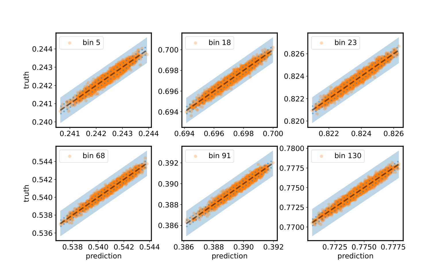
Figure 10 presents the scatter plot of the true values and the emulator-predicted values for a few randomly selected bins. Again, we see that the prediction error is well within the expected CMASS sample variance, which is shown by the blue band. The plot also shows that there is no significant bias towards the mean in the emulator prediction. Thus, we deem the best-fit neural net model to be unbiased and sufficiently accurate to replace the original likelihood calculations without introducing significant additional errors, at least within the training range.
We follow the exact same procedure for the 2PCF. We conduct tests to ensure that the resulting emulator error is subdominant compared to the data error, and that the emulator predictions are not biased towards the mean of the training range. The resulting mean emulator errors as a fraction of the data error are also around for NN() and for the 2PCF. We do not show the figures for the 2PCF for brevity.
4.4 Parameter recovery
Having trained and tested the emulators for the NNs and the 2PCF, we can test the constraints of these two summary statistics by sampling the parameter posteriors given the mock data vectors (Figure 5 and Figure 6) and the mock covariance matrices (Figure 7. For this analysis, we run three chains: one with just NN-CDF, one with just , and one with both data vectors.
For faster sampling, we use the dynesty nested sampler (Speagle & Barbary 2018; Speagle 2020). We also impose flat priors bounded with an ellipsoid for all parameters. The ellipsoid is constructed as the minimum-volume ellipsoid that envelopes all training points. We initiate each nested sampling chain with 2000 live points and a stopping criterion of , where is the evidence. As expected, we achieve excellent fits for both summary statistics, with best-fit /d.o.f .
Figure 5 and Figure 6 showcase the best fit predictions compared to the target data vectors. We achieve good fits visually in both cases. However, because the error bars on the NN-CDF are tiny on an absolute scale, we explicitly show the difference between the best fit and the target data vector in Figure 11, normalised by the CMASS error bars. We see that for most s, the best-fit residual falls well within the CMASS error. At the highest s, there is a slightly larger residual at smaller scales.
We present the resulting 2D marginalised posteriors in Figure 12 and also summarise the 1D marginalised constraints in Table 1. The blue and red contours denote the 1-2 constraints from the NNs and , respectively. The green contours showcase the joint constraints with NN+. The black lines show the truth values. The main conclusion is that our full forward model approach can obtain unbiased recoveries of all model parameters despite the layers of observational systematics. This is significant for analyses with beyond-2PCF statistics on non-linear scales as our full forward approach does not rely on any specific summary statistics. We have demonstrated that a full forward model for any summary statistic that accounts for the full range of observational systematics is computationally viable and should yield unbiased constraints.
| Parameter | Meaning | truth | post. (C.L.) | NN post. (C.L.) | joint post. (C.L.) |
|---|---|---|---|---|---|
| The typical mass scale to host a central | 12.8 | ||||
| The typical mass scale for halos to host one satellite | 13.9 | ||||
| The power-law index for satellites | 1.0 | ||||
| The incompleteness parameter | 0.41 |
Comparing the NN and 2PCF constraints, we see that the NNs derive competitive constraints compared to the 2PCF. Specifically, the NNs yield stronger constraints on while deriving slightly weaker constraints on . The fact that the NNs derive stronger constraints on shows the promise of NNs in a cosmology analysis. This is because is the only parameter controlling the occupation of the centrals since we have fixed . Given that the satellite fraction is small, the central occupation largely controls the 2-halo term in the clustering and thus the linear bias. Thus, strong constraints on translates to strong constraints on the amplitude of the linear power spectrum and the growth of structure. This is consistent with the Fisher analysis results of Banerjee & Abel 2021a.
We do, however, expect that the 2PCF would be more constraining in the satellite occupation parameters than the NNs. On the one hand, the NNs measure the counts of galaxies around randomly selected query points. In a clustered data set, the randomly selected query points will necessarily mostly sample the under-dense regions more than the over-dense regions. The 2PCF, on the other hand, measure the data-data counts, thus it necessarily samples mostly the over-dense regions, boosting the sensitivity to 1-halo scaling clustering Mpc. And because we expect the 2PCF to be more sensitive to 1-halo scale clustering, we expect it to have stronger constraints on satellite occupation parameters and . It is surprising to find the NNs to be competitive even in the satellite occupation parameters. This might be due to the fact that we include higher orders for NNs but only consider the projected 2PCF in this analysis. In our companion paper Yuan & Abel 2022, we develop variations to the standard NN formulation that exceeds the constraining power of the full-shape 2PCF, even on satellite occupation parameters.
It is also worth noting that this is not a fair comparison since we have not used the NN below Mpc (see Figure 5), whereas we used the 2PCF all the way down to Mpc. The cut on the CDF is placed to remove low signal-to-noise points in the NN and is limited by the grid spacing for the query points we used. A denser query point set would increase the signal-to-noise in the NN on small scales but allow us to meaningfully use those scales at the cost of significantly slower likelihood evaluation. In Appendix B, we present an alternative comparison of the two statistics by applying a minimum scale cut of Mpc on the 2PCF, in which case the 2PCF becomes significantly less constraining than the NNs.
Figure 12 also shows significantly stronger joint constraints when the two summary statistics are used simultaneously. This is particularly true for the satellite occupation parameters where we get an approximately factor of 2 improvement in the constraining power. The joint constraints on the central occupation parameter is not significantly stronger than the NN-CDF constraints, again demonstrating the rich information captured by the NNs. The 1D joint posteriors are again summarised in Table 1.
5 Discussions
A key limitation of this analysis is that we have only tested the recovery of HOD parameters at fixed cosmology. The goal of utilizing the full information of the smaller scales is to learn both about galaxy–halo connection and the underlying cosmology. In order to enable the cosmology dependence of the full forward model, we need simulation lightcones at non-standard cosmologies. The Quijote suite provides lightcones with variable cosmologies, but the resolution is not sufficient for modeling small scales (Villaescusa-Navarro et al. 2020). A pilot study using this suite in a forward model is described in Hahn et al. 2022b. Efforts are currently underway to produce high-fidelity lightcones at variable cosmologies from the periodic boxes of the AbacusSummit suite (Hadzhiyska et al. 2022b). We reserve the description of these products and the development of cosmology-dependent full forward models for a future paper.
The use of simulation of lightcones also enables direct modeling of redshift-dependence in the bias model, whether it be an HOD() or another galay–halo connection model. This is particularly important given the depth of current and upcoming surveys. For example, with DESI, the LRG sample is expected to span redshift range whereas the ELG sample is expected to span (Zhou et al. 2020; Raichoor et al. 2020). One clearly expects significantly redshift evolution in the galaxy–halo connection throughout these wide ranges. In a standard approach, one can divide the data into several redshift bins, and analyse each bin with a model template constructed on snapshots of the periodic box at or close to the effective redshift within each bin, such approaches suffer from potential biases due to redshift binning and covariances between different redshift bins that might be hard to account for in a combined analyses. Instead, we propose the use of our lightcone-based forward model approach where we directly parameterise the redshift evolution in the galaxy bias model and compare data to continuous mocks that span the entire redshift range. We would still need to compute the summary statistics in redshift bins, but as long as we make consistent choices between the lightcone and the data, we would not suffer from any biases due to redshift binning. The model covariance between different redshifts are also naturally accounted for. A description of redshift-dependent HOD implementaion in AbacusHOD is presented in Appendix A.
As mentioned in section 2.4.1 and section 4.1, NN analyses of galaxy–halo connection would strongly benefit from a higher density galaxy sample which would open up the smaller scales. This is particularly relevant for the DESI Bright Galaxy Survey (Hahn et al. 2022a), which will target a magnitude limited galaxy sample at . The BGS sample will go significantly fainter but denser than the LRG and ELG sample, and will be a key sample for lensing, high-order statistics, and galaxy–halo connection science. The sample will reach a number density of Mpc-3 at , i.e. 10 times that of the CMASS sample, and Mpc-3 at . Such high number density will allow the NN-CDF to probe 1-halo scales at Mpc. We also expect the BGS sample to be highly redshift-dependent. Thus, a lightcone-based forward model combined with our redshift-dependent HOD model would be the natural choice to study the BGS sample.
While lightcone-based models hold great promises, generating high-precision lightcones of sufficient volume can be a computational challenge. In this analysis, we average over 5 different lightcones (each covering an octant of the sky) at fixed cosmology to achieve the desired volume in the model and ensure the model sample variance is subdominant compared to other sources of uncertainties. With current lightcone implementations such as the one used in Hadzhiyska et al. 2022b, one can only generate one independent lightcone per simulation box. Thus for a cosmology+HOD analysis, one would require repeat simulations per cosmology or a single box that is significantly larger then what is currently available.
However, we might not need repeat lightcones to reduce sample variance after all. At small scales, sample variance is subdominant to other modeling uncertainties and observational systematics, in which case a single lightcone would be sufficient. At larger scales, there are sample variance suppression techniques such as the one developed in Kokron et al. 2022, which uses fast repeat runs of Zel’dovich codes to achieve orders of magnitude reduction to sample variance on large scales. In principle, supplementing lightcone-based predictions with this technique should result in sufficiently precise model templates across a wide range scales.
6 Conclusions
In this paper, we constructed and tested a full forward modeling pipeline for galaxy clustering statistics that utilises high-fidelity simulation lightcones and account for the full range of observational systematics. We demonstrated that one can recover unbiased model constraints using our forward modeling pipeline with the standard 2PCF and the novel -th nearest neighbor statistics (sensitive to correlation functions of all orders) on non-linear scales. While we used two summary statistics as examples, our pipeline is agnostic to the statistics used and we fully expect the technique is broadly applicable to other novel summary statistics. This is significant for analyses of upcoming cosmological surveys where the use of novel summary statistics and of non-linear scales are necessary to extract the full information content of the vast datasets.
As a part of the pipeline, we also introduced a novel treatment of fibre collision effects. Specifically, we use the measured clustering to probabilistically recover the redshifts of fibre collided targets. We tested this technique on both the projected 2PCF and the NNs and found good redshift recovery compared to other systematics budget. This method is promising as it does not appeal to any specific properties of summary statistics and is in principle applicable to a wide array of beyond-2PCF analyses. We propose additional testing of the method and potential enhancements by leveraging additional information, such as combining with photometric redshift inferences.
By testing our pipeline with two different summary statistics, we also produced a realistic comparison of the -th nearest neighbor statistics to the standard 2PCF. We showed that the NNs derive stronger constraints on the linear bias, and the two statistics are similarly informative of the properties of satellite galaxies. We explore additional variations to the NN formalism in the companion paper Yuan & Abel 2022.
Acknowledgements
We would like to thank Risa Wechsler, Arka Banerjee, Ashley Ross, Sebastian Wagner-Carena, Philip Mansfield for useful feedback and suggestions in various stages of this analysis.
This work was supported by U.S. Department of Energy through grant DE-SC0013718 and under DE-AC02-76SF00515 to SLAC National Accelerator Laboratory.
This work used resources of the National Energy Research Scientific Computing Center (NERSC), a U.S. Department of Energy Office of Science User Facility located at Lawrence Berkeley National Laboratory, operated under Contract No. DE-AC02-05CH11231.
The AbacusSummit simulations were conducted at the Oak Ridge Leadership Computing Facility, which is a DOE Office of Science User Facility supported under Contract DE-AC05-00OR22725, through support from projects AST135 and AST145, the latter through the Department of Energy ALCC program.
Data Availability
The simulation data are available at https://abacussummit.readthedocs.io/en/latest/. The AbacusHOD code package is publicly available as a part of the abacusutils package at http://https://github.com/abacusorg/abacusutils. Example usage can be found at https://abacusutils.readthedocs.io/en/latest/hod.html.
References
- Abareshi et al. (2022) Abareshi B., et al., 2022, arXiv e-prints, p. arXiv:2205.10939
- Alcock & Paczynski (1979) Alcock C., Paczynski B., 1979, Nature, 281, 358
- Anderson et al. (2012) Anderson L., et al., 2012, MNRAS, 427, 3435
- Anderson et al. (2014) Anderson L., et al., 2014, MNRAS, 441, 24
- Banerjee & Abel (2021a) Banerjee A., Abel T., 2021a, MNRAS, 500, 5479
- Banerjee & Abel (2021b) Banerjee A., Abel T., 2021b, MNRAS, 504, 2911
- Bianchi & Percival (2017) Bianchi D., Percival W. J., 2017, MNRAS, 472, 1106
- Bianchi et al. (2018) Bianchi D., et al., 2018, MNRAS, 481, 2338
- Blanton et al. (2003) Blanton M. R., Lin H., Lupton R. H., Maley F. M., Young N., Zehavi I., Loveday J., 2003, AJ, 125, 2276
- Carlson et al. (2009) Carlson J., White M., Padmanabhan N., 2009, Phys. Rev. D, 80, 043531
- Carlson et al. (2013) Carlson J., Reid B., White M., 2013, MNRAS, 429, 1674
- Chapman et al. (2021) Chapman M. J., et al., 2021, arXiv e-prints, p. arXiv:2106.14961
- D’Amico et al. (2022) D’Amico G., Donath Y., Lewandowski M., Senatore L., Zhang P., 2022, arXiv e-prints, p. arXiv:2206.08327
- DESI Collaboration et al. (2016) DESI Collaboration et al., 2016, arXiv e-prints, p. arXiv:1611.00036
- Dawson et al. (2013) Dawson K. S., et al., 2013, AJ, 145, 10
- Dawson et al. (2016) Dawson K. S., et al., 2016, AJ, 151, 44
- Eisenstein et al. (2005) Eisenstein D. J., et al., 2005, ApJ, 633, 560
- Garrison et al. (2019) Garrison L. H., Eisenstein D. J., Pinto P. A., 2019, MNRAS, 485, 3370
- Garrison et al. (2021) Garrison L. H., Eisenstein D. J., Ferrer D., Maksimova N. A., Pinto P. A., 2021, MNRAS, 508, 575
- Garrison et al. (2022) Garrison L. H., Abel T., Eisenstein D. J., 2022, MNRAS, 509, 2281
- Gil-Marín et al. (2017) Gil-Marín H., Percival W. J., Verde L., Brownstein J. R., Chuang C.-H., Kitaura F.-S., Rodríguez-Torres S. A., Olmstead M. D., 2017, MNRAS, 465, 1757
- Guo et al. (2012) Guo H., Zehavi I., Zheng Z., 2012, ApJ, 756, 127
- Guo et al. (2015) Guo H., et al., 2015, MNRAS, 446, 578
- Guo et al. (2018) Guo H., Yang X., Lu Y., 2018, ApJ, 858, 30
- Hadzhiyska et al. (2022a) Hadzhiyska B., Eisenstein D., Bose S., Garrison L. H., Maksimova N., 2022a, MNRAS, 509, 501
- Hadzhiyska et al. (2022b) Hadzhiyska B., Garrison L. H., Eisenstein D., Bose S., 2022b, MNRAS, 509, 2194
- Hahn et al. (2017) Hahn C., Scoccimarro R., Blanton M. R., Tinker J. L., Rodríguez-Torres S. A., 2017, MNRAS, 467, 1940
- Hahn et al. (2022a) Hahn C., et al., 2022a, arXiv e-prints, p. arXiv:2208.08512
- Hahn et al. (2022b) Hahn C., et al., 2022b, arXiv e-prints, p. arXiv:2211.00723
- Hamilton & Tegmark (2004) Hamilton A. J. S., Tegmark M., 2004, MNRAS, 349, 115
- Heitmann et al. (2009) Heitmann K., Higdon D., White M., Habib S., Williams B. J., Lawrence E., Wagner C., 2009, ApJ, 705, 156
- Heitmann et al. (2014) Heitmann K., Lawrence E., Kwan J., Habib S., Higdon D., 2014, ApJ, 780, 111
- Jiménez et al. (2019) Jiménez E., Contreras S., Padilla N., Zehavi I., Baugh C. M., Gonzalez-Perez V., 2019, MNRAS, 490, 3532
- Kobayashi et al. (2022) Kobayashi Y., Nishimichi T., Takada M., Miyatake H., 2022, Phys. Rev. D, 105, 083517
- Kokron et al. (2022) Kokron N., Chen S.-F., White M., DeRose J., Maus M., 2022, arXiv e-prints, p. arXiv:2205.15327
- Kwan et al. (2015) Kwan J., Heitmann K., Habib S., Padmanabhan N., Lawrence E., Finkel H., Frontiere N., Pope A., 2015, ApJ, 810, 35
- Landy & Szalay (1993) Landy S. D., Szalay A. S., 1993, ApJ, 412, 64
- Lange et al. (2022) Lange J. U., Hearin A. P., Leauthaud A., van den Bosch F. C., Guo H., DeRose J., 2022, MNRAS, 509, 1779
- Lawrence et al. (2010) Lawrence E., Heitmann K., White M., Higdon D., Wagner C., Habib S., Williams B., 2010, ApJ, 713, 1322
- Leauthaud et al. (2016) Leauthaud A., et al., 2016, MNRAS, 457, 4021
- Levi et al. (2013a) Levi M., et al., 2013a, arXiv e-prints, p. arXiv:1308.0847
- Levi et al. (2013b) Levi M., et al., 2013b, arXiv e-prints, p. arXiv:1308.0847
- Li et al. (2006) Li C., Kauffmann G., Jing Y. P., White S. D. M., Börner G., Cheng F. Z., 2006, MNRAS, 368, 21
- Maksimova et al. (2021) Maksimova N. A., Garrison L. H., Eisenstein D. J., Hadzhiyska B., Bose S., Satterthwaite T. P., 2021, MNRAS,
- Ménard et al. (2013) Ménard B., Scranton R., Schmidt S., Morrison C., Jeong D., Budavari T., Rahman M., 2013, arXiv e-prints, p. arXiv:1303.4722
- Mohammad et al. (2020) Mohammad F. G., et al., 2020, MNRAS, 498, 128
- Pellejero-Ibañez et al. (2020) Pellejero-Ibañez M., Angulo R. E., Aricó G., Zennaro M., Contreras S., Stücker J., 2020, MNRAS, 499, 5257
- Pinol et al. (2017) Pinol L., Cahn R. N., Hand N., Seljak U., White M., 2017, J. Cosmology Astropart. Phys., 2017, 008
- Raichoor et al. (2020) Raichoor A., et al., 2020, Research Notes of the American Astronomical Society, 4, 180
- Reid et al. (2016) Reid B., et al., 2016, MNRAS, 455, 1553
- Rodríguez-Torres et al. (2016) Rodríguez-Torres S. A., et al., 2016, MNRAS, 460, 1173
- Ross et al. (2012) Ross A. J., et al., 2012, MNRAS, 424, 564
- Ross et al. (2015) Ross A. J., Percival W. J., Manera M., 2015, MNRAS, 451, 1331
- Sheth & van de Weygaert (2004) Sheth R. K., van de Weygaert R., 2004, MNRAS, 350, 517
- Sinha & Garrison (2020) Sinha M., Garrison L. H., 2020, MNRAS, 491, 3022
- Sinha et al. (2018) Sinha M., Berlind A. A., McBride C. K., Scoccimarro R., Piscionere J. A., Wibking B. D., 2018, MNRAS, 478, 1042
- Slepian et al. (2017a) Slepian Z., et al., 2017a, MNRAS, 468, 1070
- Slepian et al. (2017b) Slepian Z., et al., 2017b, MNRAS, 469, 1738
- Smith et al. (2019) Smith A., et al., 2019, MNRAS, 484, 1285
- Speagle (2020) Speagle J. S., 2020, MNRAS, 493, 3132
- Speagle & Barbary (2018) Speagle J., Barbary K., 2018, dynesty: Dynamic Nested Sampling package, Astrophysics Source Code Library (ascl:1809.013)
- Storey-Fisher et al. (2022) Storey-Fisher K., Tinker J., Zhai Z., DeRose J., Wechsler R. H., Banerjee A., 2022, arXiv e-prints, p. arXiv:2210.03203
- Swanson et al. (2008) Swanson M. E. C., Tegmark M., Hamilton A. J. S., Hill J. C., 2008, MNRAS, 387, 1391
- Takada et al. (2014) Takada M., et al., 2014, PASJ, 66, R1
- Tam et al. (2022) Tam S.-I., Umetsu K., Amara A., 2022, ApJ, 925, 145
- Valogiannis & Dvorkin (2022a) Valogiannis G., Dvorkin C., 2022a, arXiv e-prints, p. arXiv:2204.13717
- Valogiannis & Dvorkin (2022b) Valogiannis G., Dvorkin C., 2022b, Phys. Rev. D, 105, 103534
- Villaescusa-Navarro et al. (2020) Villaescusa-Navarro F., et al., 2020, ApJS, 250, 2
- Wechsler et al. (2022) Wechsler R. H., DeRose J., Busha M. T., Becker M. R., Rykoff E., Evrard A., 2022, ApJ, 931, 145
- White (2016) White M., 2016, J. Cosmology Astropart. Phys., 2016, 057
- White & Padmanabhan (2009) White M., Padmanabhan N., 2009, MNRAS, 395, 2381
- Yuan & Abel (2022) Yuan S., Abel T., 2022, in prep.
- Yuan et al. (2018) Yuan S., Eisenstein D. J., Garrison L. H., 2018, MNRAS, 478, 2019
- Yuan et al. (2021) Yuan S., Garrison L. H., Hadzhiyska B., Bose S., Eisenstein D. J., 2021, MNRAS, 510, 3301
- Yuan et al. (2022a) Yuan S., Garrison L. H., Eisenstein D. J., Wechsler R. H., 2022a, MNRAS,
- Yuan et al. (2022b) Yuan S., Hadzhiyska B., Bose S., Eisenstein D. J., 2022b, MNRAS, 512, 5793
- Zhai et al. (2019) Zhai Z., et al., 2019, ApJ, 874, 95
- Zhai et al. (2022) Zhai Z., et al., 2022, arXiv e-prints, p. arXiv:2203.08999
- Zheng et al. (2005) Zheng Z., et al., 2005, ApJ, 633, 791
- Zheng et al. (2007) Zheng Z., Coil A. L., Zehavi I., 2007, ApJ, 667, 760
- Zhou et al. (2020) Zhou R., et al., 2020, Research Notes of the American Astronomical Society, 4, 181
Appendix A redshift-dependent HOD
The AbacusHODpackage also enables populating lightcones with redshift-dependent HODs. This is particularly powerful for current and future deep surveys such as DESI and PFS that observe galaxies over a large redshift range. In such samples, modeling redshift evolution not only helps our understanding of galaxy evolution, but also is necessary to avoid biasing the cosmology constraints and thus leverage the full statistical power of the data.
In a first implementation, we add two additional free parameters to the model, and , where we define . These two parameters are the first derivative of and against the scale factor, respectively. Thus, the modified parameters in the AbacusHOD model take the following form for a given choice of a reference redshift, ,
| (9) |
where . Currently, we opt to make only and redshift-dependent for simplicity. In principle, all HOD parameters can be redshift-dependent and the AbacusHOD package can be easily extended to accommodate such complexities.
Appendix B Comparing the statistics on equivalent scales
Figure 12 appears to show the 2PCF as more informative on the HOD than NNs. However, as we pointed out towards the end of section 4.4, we have only utilised the NNs on scales above Mpc due to the relatively sparse query set, whereas we used the 2PCF all the way down to Mpc. Here we facilitate a comparison of the two statistics at equivalent scales, specifically by only using the 2PCF at scales Mpc. We follow the exact same procedure as laid out in section 4 and show the resulting constraints in Figure 13.
We see that the constraining power of the projected 2PCF decreases considerably in both the central and satellite HOD parameters. The constraints on the satellite parameter turns out particularly poor, hitting prior bounds in both directions. The at Mpc still derives strong constraints on the mass parameters and , but the constraining power is now significantly inferior to that of the NN.
Finally, we note that the definition of scales is different between the 2PCF and NNs, with the 2PCF defining the separation between data-data pairs and NNs defining the separation between data-query pairs. The idea of testing on equivalent scales is an attempt to compare the statistics in roughly the same 2-halo regime, but an exactly fair comparison is not possible. We also point to the fact that there are significantly more bins available in the NN than the projected 2PCF. Ultimately, these results highlight the complementarity of the two statistics and the potential information gain by combining the two.