Phase Transitions in Learning and Earning under Price Protection Guarantee
Abstract
Motivated by the prevalence of “price protection guarantee”, which allows a customer who purchased a product in the past to receive a refund from the seller during the so-called price protection period (typically defined as a certain time window after the purchase date) in case the seller decides to lower the price, we study the impact of such policy on the design of online learning algorithm for data-driven dynamic pricing with initially unknown customer demand. We consider a setting where a firm sells a product over a horizon of time steps. For this setting, we characterize how the value of , the length of price protection period, can affect the optimal regret of the learning process. We show that the optimal regret is by first establishing a fundamental impossible regime with novel regret lower bound instances. Then, we propose LEAP, a phased exploration type algorithm for Learning and EArning under Price Protection to match this lower bound up to logarithmic factors or even doubly logarithmic factors (when there are only two prices available to the seller). Our results reveal the surprising phase transitions of the optimal regret with respect to . Specifically, when is not too large, the optimal regret has no major difference when compared to that of the classic setting with no price protection guarantee. We also show that there exists an upper limit on how much the optimal regret can deteriorate when grows large. Finally, we conduct extensive numerical experiments to show the benefit of LEAP over other heuristic methods for this problem.
keywords
dynamic pricing, online learning, price protection, exploration-exploitation tradeoffqf48@cornell.edu SC Johnson College of Business, Cornell University
ruihao.zhu@cornell.edu Stephen M. Ross School of Business, University of Michigan
sjasin@umich.edu ††affiliation: ††affiliation: ††affiliation: ††affiliation: ††affiliation: ††affiliation:
1 Introduction
Rapid development of data science technologies have enabled the incorporation of data-driven decision-making into revenue management. Among others, one of the most successful and prevalent examples is online learning for data-driven dynamic pricing (Kleinberg and Leighton 2003, Harrison et al. 2012, Keskin and Zeevi 2014). In the classic formulation of this problem, there is a firm, hereafter referred to as the seller, who sells a single product to customers over a time horizon without knowing their response to different prices ahead. The seller aims at maximizing her expected total revenue, but she faces the exploration-exploitation (a.k.a. learning and earning) tradeoff: On the one hand, she has to offer different prices to estimate the demand (response) of the customers; on the other hand, she also needs to choose the optimal price to maximize her expected total revenue. For this problem and many of its variants, many works in the literature have developed (nearly) optimal online learning algorithms to strike the right balance between exploration and exploitation (interested readers are referred to den Boer 2015 for a comprehensive survey). To date, companies from different industries, including e-commerce (Mehta et al. 2018), retailing (Bond 2022), and many others, have deployed data-driven dynamic pricing methods to gain more revenue.
In the traditional data-driven dynamic pricing literature, it is typically assumed that the seller can adjust the price as frequently as she wishes. In practice, however, as has been frequently reported (see, e.g., Bondi et al. 2021, Sivakumar 2022), customers can find it frustrating and unfair if the price of a recently purchased product drops to a lower level shortly afterward. This can further cause negative reviews due to customer dissatisfaction and, even worse, customer alienation. Consequently, it becomes clear that directly applying data-driven dynamic pricing in its canonical form may not be beneficial in the long run (Mohammed 2012).

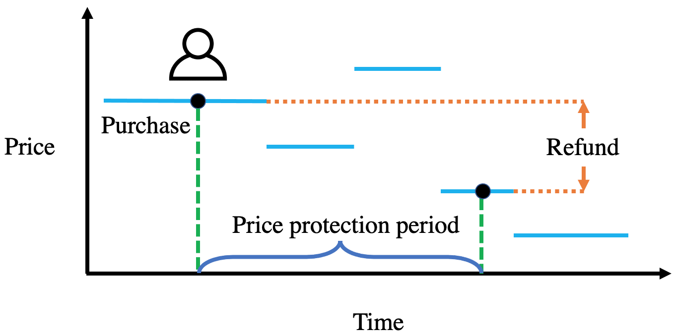
As a (partial) remedy for the inconvenience created by dynamic pricing, many companies have now implemented some forms of price protection guarantees (either explicitly or implicitly) for their products (see Figure 1 for some examples). In a nutshell, such price protection guarantee allows a customer who purchased a product in the past to receive a refund from the seller during the so-called price protection period (typically defined as a certain time window after the purchase date) in case the seller decides to lower the price. Here, the amount of refund is equal to the difference between the price paid and the lowest price found within the price protection period. For example, in Figure 2, suppose for a certain period of time, the seller uses five different prices , and (in descending order), and the customer purchases the product at . Then, thanks to price protection, she will receive a refund of amount so that her actual payment is , which is the lowest price found during the price protection period 11 1 We remark that although some companies only refund customers once during the price protection period while others allow multiple refunds if price drops further, we restrict our attention to the latter for brevity. Our forthcoming results, however, shall be mostly applicable to the former as well.22 2 If multiple price drops occur during the price protection period, one can assume that the customers receive the respective refunds all at once at the end of the price protection period. Alternatively, we could also assume that the customers receive refunds immediately after each price drop. Since the total amount of refunds are the same in both cases, we do not distinguish one from another throughout..
1.1 Main Contributions
While price protection has now become one of the industry standards, its impact on data-driven dynamic pricing, especially on the corresponding online learning process, remains largely unexplored. In this paper, we provide an initial characterization of this effect.
Let be the total number of time steps and be the length of price protection period. Our results and contributions can be summarized as follows:
- 1.
Due to the existence of price protection, directly applying classic approaches that ignores price protection such as Upper Confidence Bound (UCB) algorithm Auer et al. 2002b and Thompson Sampling algorithm Agrawal and Goyal 2012 would suffer linear in regret. We use both theoretical and numerical evidences to support this claim.
- 2.
As such, we begin with the case where there are only two prices available to the seller. We show that the optimal regret is by first establishing a theoretical lower bound. Both of our lower bound instances and the proof techniques are different than traditional regret lower bounds (see the forthcoming Remark 3 for a detailed discussion). Next, we develop LEAP, a novel phased exploration algorithm for Learning and EArning under Price Protection to match this lower bound up to factors. To achieve this, LEAP creatively implements asynchronous price exploration and price elimination schedules. This mechanism allows us to simultaneously avoid excessive refunds and excessive selection of sub-optimal price (see the forthcoming Remark 5 for a detailed discussion). After we complete the analysis for the case with only two price points, we generalize our results to the case with multiple price points and establish the optimal (up to logarithmic factors) regret. We refer to Table 1 for a summary.
Number of prices 2 Regret lower bound Regret upper bound Table 1: Optimal regret of our problem - 3.
Importantly, our results reveal the surprising phase transitions of the optimal regret with respect to the length of price protection period . Specifically, when , price protection has no major effect on the optimal regret when compared to the case without it. When , the optimal regret scales linearly with while, when , the optimal regret would remain at the level of , which serves as an upper limit on the deterioration caused to the optimal regret by price protection guarantee. As the value of varies among different companies, our results is useful for informing the implementation of price protection policy in practice.
- 4.
Finally, we conduct extensive numerical experiments to show that, by properly coordinating price protection and learning, our proposed algorithms are able to achieve significant improvement compared to other benchmark heuristic methods in our setting.
1.2 Related Work
In this section, we provide a detailed review of prior related studies. We start by reviewing existing works in online learning for classic dynamic pricing. Next, we discuss some connections between our setting and that of dynamic pricing in the face of strategic customers. Finally, we discuss existing works in the context of multi-armed bandits with limited adaptivity. Throughout, we will highlight the similarity and key differences between our work and prior works.
Online Learning for Dynamic Pricing: Online learning for dynamic pricing has been intensively studied in the literature, given its wide applications in retailing and e-commerce (den Boer 2015, Ferreira et al. 2016). Many papers have developed near-optimal algorithms for pricing a product over multiple time periods under various settings (see, e.g., Kleinberg and Leighton 2003, Besbes and Zeevi 2009, Araman and Caldentey 2009, Farias and Van Roy 2010, Harrison et al. 2012, Broder and Rusmevichientong 2012, den Boer and Zwart 2014, Keskin and Zeevi 2014, Wang et al. 2014, Keskin and Zeevi 2016, Ferreira et al. 2018, Cohen et al. 2021, Chen and Gallego 2021, Wang et al. 2021, Cheung et al. 2021, Zhu and Zheng 2021, Bastani et al. 2022, Simchi-Levi et al. 2022, Bu et al. 2022). In recent years, there has also been increasing interests in dynamic pricing by taking into account exogenous and/or personalized features (see, e.g., Qiang and Bayati 2016, Javanmard and Nazerzadeh 2019, Keskin et al. 2022, Ban and Keskin 2021, Chen et al. 2022b, Li and Zheng 2019). Different from the above classic works, we mainly focus on online learning for dynamic pricing under price protection.
Dynamic Pricing under Strategic Customers: Our work is closely related to the literature of dynamic pricing in the presence of strategic and patient customers. In the latter, it generally assumes that customers can observe prices throughout a certain period of time, and then purchase at the lowest price possible (see, e.g., Feldman et al. 2016, Birge et al. 2021, Chen et al. 2022a, Zhang and Jasin 2022, and references therein). Prior works show that strategic and patient customers present extra challenge to the seller and may incur larger regret. For example, Birge et al. 2021 studies the markdown pricing problem of a firm that sells a product to a set of myopic and forward-looking customers. Birge et al. 2021 shows the seller’s revenue under demand model uncertainty and strategic customers depends crucially on how forward-looking the customers are. In particular, when the customers’ forward-looking behavior is exogenous and their memory is unbounded, the seller has to suffer a major revenue loss. The authors also characterize conditions under which the seller can achieve asymptotic optimality. Our setting differs from Birge et al. 2021 in several aspects. First, we study a frequentist setting where there is no prior belief over the customer demand models while Birge et al. 2021 studies a Bayesian setting where there is a prior over potential customer demand models. Also, Birge et al. 2021 considers the customers to be forward-looking and they are capable of predicting the future prices of the product. In contrast, our setting assumes the customers would make an instantaneous purchase decision, and then passively receive the refunds from the price protection guarantee. Finally, we do not impose the restriction that the seller can only mark down the price over time.
Feldman et al. 2016 shows in the adversarial setting (i.e., customer demand may not follow a stationary distribution) that if customers can observe the prices for several time steps and wait for the lowest price, then the optimal regret for the seller would become instead of in classic dynamic pricing. Our setting is similar to Feldman et al. 2016 in that customers effectively also pay the lowest price within certain time duration. But we are critically different in that we consider a less pessimistic scenario where the random demand follows a stochastic distribution, and the oracle policy (when the demand distribution is known ahead) can be easily identified.
Zhang and Jasin 2022 studies the setting where customers are patient and are willing to wait for a few periods before deciding to leave the system without making any purchase. Specifically, each customer is endowed with a (potentially different) willingness to pay and willingness to wait, and a customer will buy the product at the first time the price is smaller than or equal to the customer’s willingness to pay. Zhang and Jasin 2022 develops several near-optimal cyclic pricing policy. They also show that standard learning algorithms that ignore patient customer behavior will suffer a significant loss in revenue. Our setting differs from Zhang and Jasin 2022 in at least one crucial component: Since Zhang and Jasin 2022 assumes that a customer will buy the product at the first time the price is smaller than or equal to the customer’s willingness to pay, this price may not be the smallest price within the time periods in which the customer is willing to wait. Moreover, unlike in their setting, the optimal pricing policy in our setting is not cyclic.
Multi-armed Bandits with Limited Adaptivity: From a technical point of view, our setting is related to multi-armed bandits with limited adaptivity (e.g., Gao et al. 2019, Simchi-Levi and Xu 2021, Rouyer et al. 2021). This is so because, in our setup, whenever there is a price decrease, the seller may have to refund the customers. This would implicitly refrain the seller from changing the price. In Simchi-Levi and Xu 2021 and Gao et al. 2019, the authors impose a restriction that the decision-maker (which is the seller in our setting) can only change her actions/policies (which is price in our setting) up to a pre-specified number of times. Simchi-Levi and Xu 2021 reveals an interesting phase transition behavior of the optimal regret w.r.t. the number of changes allowed. Moreover, both papers confirm that (doubly) logarithmic amount of adaptivity would be enough to attain the optimal regret. As a matter of fact, part of our optimal learning strategy to plan pricing in batches (i.e., minimizing the number of price changes) is motivated by Simchi-Levi and Xu 2021 and Gao et al. 2019. However, different than this line of work, there is no explicit constraint on the number of price changes in our model. Instead, this constraint enters the play implicitly as a kind of regularization. It turns out that this difference leads to drastically different results, from algorithm design to the phase transitions of the optimal regret. We refer to Section 4.3 for more detailed discussions.
In Rouyer et al. 2021, the authors assume that a unit cost would be incurred whenever an action change takes place. Similar to Rouyer et al. 2021, the cost of price changes in our setting is incorporated into the objective function as a regularization. In some sense, results for stochastic bandits with switching cost developed in Rouyer et al. 2021 can be viewed as a special case of our results with .
2 Problem Formulation
In this section, we introduce the notations that will be be used throughout paper. In addition, we will also introduce the learning protocol for our problem.
2.1 Notations
We define to be the set for any positive integer For , we use to denote the -norm of a vector We use to denote the logarithm with base When is left unspecified, this is the natural logarithm. We adopt the asymptotic notations and as defined in (Cormen et al. 2009). When logarithmic factors are omitted, we write them as and With some abuse, these notations are used when we try to avoid the clutter of writing out constants explicitly. The indicator variable is denoted as
2.2 Model
Model Primitives: We consider a firm, hereafter refereed to as the seller, that sells a single product over a horizon of time steps. For each time step the seller must first set a price and then observes the i.i.d. customer demand We let be the initially unknown expected demand w.r.t. price We use to denote the expected reward of offering price for For ease of exposition, we often refer to as price To simplfy notation, we define for all whenever or
Price Protection Guarantee: Motivated by practice, we assume that the seller provides price protection guarantee for a total of time steps. That is, even if a customer purchases the product in time step at an initial price her final payment would be the minimum among the prices of this period and the immediate next time periods, i.e., In other words, she would be refunded the difference between and the minimum of
Objective: Since the actual payment of a customer who arrives at time step is , the total revenue of the seller throughout the entire time horizon can be written as
and the total refund throughout the horizon can be written as
It is also useful to think of revenue from an instantaneous point of view. At time step , if the seller sets the price to , then she will receive an instantaneous reward (i.e., payment) of . At the same time, this decision may also incur refunds for customers arriving between time step to time step . Consider any time step satisfying . By time the end of time step , the actual payment of the customer arriving at time period is . Therefore, if is selected at time period , the additional refund for the customer of time step is . This means the net revenue at time period for the seller when selecting can be written as
| (1) |
We denote the second term, i.e., the instantaneous refund, as .
The objective of the seller is to maximize her expected cumulative revenue by following a possibly randomized non-anticipatory pricing policy Specifically, denoting as the history at time at each time step the seller follows to pick a price We use the notion of expected regret to measure the performance of the seller. Specifically, regret is defined as the difference between the maximum expected cumulative revenue of the seller could attain should her knows all ’s ahead (note that, in this case, the seller would follow a fixed price policy, see Remark 1 for more details) and the cumulative revenue of i.e.,
| (2) |
We point out that the regret in our setting shall depend on both and but we avoid the explicit dependence for notational brevity.
Remark 1.
If there is no price protection, the optimal policy for a seller with full knowledge of all ’s would be constantly selecting the price with the highest . If the seller follows the same policy in the case with price protection, she would still achieve the maximum expected revenue (i.e., since no refund would be incurred). Hence, under price protection, the optimal policy is still constantly selecting the price with highest when all ’s are known to the seller.
Additional Notations: To facilitate our discussion, for any time step we will use to denote the number of times that price is selected up to the beginning of time step i.e.,
The corresponding empirical mean of up to the beginning of time step is denoted as
2.3 Blooper Reel
In this section, to provide an initial, but concrete understanding of the challenges of data-driven dynamic pricing in the presence of price protection guarantee, we consider two celebrated dynamic pricing algorithms, the Upper Confidence Bound (UCB) algorithm (Auer et al. 2002b, Kleinberg and Leighton 2003) and the Thompson Sampling (TS) algorithm (Agrawal and Goyal 2012). It is well known that, in absence of the price protection mechanism, both the UCB and the TS algorithms are capable of attaining the minimax optimal regret (i.e., ) for the classic problem of dynamic pricing. Due to their proximity, it is tempting to apply the UCB and the Thompson Sampling algorithms to our problem. However, as we show below, a direct application of the UCB algorithm can result in linear regret even when the price protection period is small.
We first discuss the popular UCB algorithm introduced in Auer et al. 2002b: For each time step UCB selects the price that maximizes the index i.e.,
| (3) |
The following proposition tells us that the above UCB algorithm could incur regret even when the price protection period is small.
Proposition 1.
Suppose that and there are only two prices . Then, there exists a demand distribution such that UCB algorithm will incur regret.
[Proof Sketch] The complete proof of this proposition is given in Section A.1 of the Appendix. In a nutshell, we provide an instance of demand distributions such that if , then UCB would pick as the difference between and (i.e., the second terms in (3)) would dominate the difference between and (i.e., the first terms in (3)) and vice versa. Consequently, UCB would alternate between and , which would incur regret (due to refund under price protection).
Remark 2 (Further Discussions on UCB).
In Section A.2 of the Appendix, we provide numerical examples to support the claim in Proposition 1. It is evident that the results in Proposition 1 can be easily generalized to more than two prices, i.e., Moreover, it turns out that the above findings can go beyond the canonical UCB. In Section A.3 of the Appendix, we provide further discussions on how even a general family of UCB algorithm can fail to provide meaningful performance guarantee under the price protection mechanism.
We also use numerical examples to further demonstrate that both the UCB algorithm (Auer et al. 2002b) and the Thompson Sampling algorithm (Agrawal and Goyal 2012) incur linear regret due to the price protection mechanism. Specifically, we use the following instance. (i.e., there are only two prices), with The demand under the two prices are In this case, the expected reward of selecting and are and respectively. The time horizon varies from to with a step size of and the length of price protection period is set to be For each , we compute the expected regret by averaging over iterations. The results are shown in Figure 3(a), and the portion of (expected) refund in (expected) regret under different is shown in Figure 3(b). Typical sample paths of UCB and Thompson Sampling on this instance when are shown in Figure 3(c) and Figure 3(d).


From Figure 3(a), one can see that the expected regrets of the UCB and the Thompson Sampling algorithms scale linearly with Furthermore, one can see from Figure 3(b) that refund takes up of more than of regret throughout, which indicates that the majority of the regret comes from the refund under the price protection mechanism.
One reason that both UCB and Thompson Sampling incur linear regrets is as follows: Although both algorithms select more frequently, they do not completely eliminate the selection of . Whenever is selected, a major refund would be incurred. As can be seen from Figure 3(c) and Figure 3(d), selecting , especially when gets large, would cause a refund for almost all time steps before that. Since , both UCB or Thompson sampling thus incur linear in regret.
To this end, one might be curious if a simple modification of the UCB and the Thompson Sampling, which take the price protection mechanism into account, could resolve the issue. We conduct further numerical experiments in the forthcoming Section 5.1 to show that even a natural modification of either UCB or Thompson Sampling algorithm that that takes into account refund would still incur linear regret.
3 Price Protection with Two Prices: A First Look
The above discussions show that the presence of price protection guarantee can dramatically change the landscape of the dynamic pricing problem from its classical form. Most importantly, directly applying existing algorithms designed for the setting without price protection guarantee to our setting can generate highly unsatisfactory performance.
In particular, the price protection guarantee creates an extra layer of difficulty to the dynamic pricing problem as any (unnecessary) decrease of price may result in undesirable loss of revenue. At the same time, in order to identify the optimal price, experimenting among different prices is indispensable Gao et al. 2019, Simchi-Levi and Xu 2021 (we refer the readers to the forthcoming Remark 4 and Section 4.3 for a comparison between the two settings).
To gain some preliminary insights on how to strike the right balance between exloration and exploitation, we begin with the case where there are only two candidate prices, i.e., and Without loss of generality, we assume that In Section 3.1, we characterize a theoretical lower bound, which establishes a fundamental impossibility result for the special case with two prices. Next, we turn our attention to regret minimization. In Section 3.2, we propose LEAP, an algorithm for Learning and EArning under Price protection. LEAP is a phased exploration type algorithm that judiciously balances exploration, exploitation, and price adjustment (see the forthcoming Remark 4 for intuition on this design). In each phase, it explores both prices according to a pre-specified price exploration schedule, and it also has a -dependent price elimination schedule. Specifically, when is not too large (i.e., ), these two schedules are asynchronous, i.e., price elimination can happen in the middle of a phase of price exploration. This turns out to be beneficial in further reducing expected regret when compared to the synchronous design, and may be of independent interest (see the forthcoming Remark 5 for a detailed discussion on this design). When is large (i.e., ), these two schedules are synchronous and LEAP becomes similar to the explore-then-commit algorithm (see, e.g., chapter 6 of Lattimore and Szepesvári 2020), which could help to avoid excessive refund. In Section 3.3, we analyze the expected regret upper bound of LEAP, and compare its design against classic phased exploration algorithms for learning and earning (see, e.g., Auer and Ortner 2010). Combining the above, our results indicate that the upper and lower bound match each other up to factor. Most surprisingly, under the two price case, the optimal regret for our problem exhibits different growing patterns w.r.t. different ranges of price protection period which we refer to as the phase transition phenomenon. We provide an in-depth discussion for this finding in Section 3.4.
3.1 Lower Bound
Below, we establish a theoretical lower bound, which presents a fundamental impossibility regime for our problem.
Theorem 1.
For any and any non-anticipatory policy , there exists and the corresponding distributions of demand such that the regret of is
[Proof Sketch.] The complete proof is provided in Section B of the Appendix. Depending on the value of we distinguish three different cases.
Case 1. For this case, one can use the standard lower bound argument for multi-armed bandit (see, e.g., Theorem 5.1 of Auer et al. 2002a) to show that the lower bound is .
Case 2. For this case, we assume the demand of is deterministic and known in advance, and we come up with two different choices of demand for In instance 1, selecting would bring lower expected payment than selecting while in instance 2, selecting would bring higher expected payment than selecting
As such, if a policy selects for times before some time period such that, it would not be able to distinguish which instance is presented and suffers expected regret if instance 2 is presented; while if it selects for times before time period then either the price protection guarantee or the avoidance of refund (i.e., by not selecting ) during the last time steps would also incur expected regret if instance 1 is presented.
Case 3. The proof for this case is similar to that of Case 2 except that in instance 1, selecting would bring lower expected payment than selecting while in instance 2, selecting would bring higher expected payment than selecting
As such, if a policy selects for times before some time period it would not be able to distinguish which instance is presented and suffers expected regret if instance 2 is presented; while if it selects for before time period then either the price protection mechanism or the avoidance of refund (i.e., by not selecting ) during the last time steps would also incur expected regret if instance 1 is presented.
Remark 3 (Novelty of Our Regret Lower Bound).
Despite the connections between our setting and the standard multi-armed bandits, our lower bound proof is different from the classic lower bound proof for multi-armed bandits in a subtle, yet critical way. To see this more clearly, in both Case 2 and Case 3 above, we distinguish two different sub-cases based on the exact number of times is selected (i.e., ) instead of the expected number of times is selected (i.e., ), as in Theorem 5.1 of Auer et al. 2002a or Theorem 15.2 of Lattimore and Szepesvári 2020. It turns out that this subtle difference is extremely important in making sure that the price protection guarantee can incur adequate refund. Otherwise, in Case 2 above, for instance, suppose a policy only has . Even if it keeps selecting after time step the expected regret incurred by the price protection guarantee could be as low as (this happens if is a policy such that with probability while with probability ). Associated with these are a set of carefully designed information-theoretic tools different from those in Auer et al. 2002a and Lattimore and Szepesvári 2020. We refer interested readers to Section B.2 of the Appendix for a more involved discussion.
3.2 Algorithm for Learning and Earning under Price Protection (LEAP)
In the previous discussions in Section 2.3, we can observe that ordinary learning and earning strategies cannot achieve meaningful regret guarantee because they do not take the price protection guarantee into account. To this end, we develop LEAP, which explores the two prices in phases (of possibly increasing length), and eliminates the under-performing price once its detected. The formal description of LEAP is provided in Algorithm 1. It follows different steps w.r.t. different values of . We discuss the two cases and separately below.
Case 1.
In this case, LEAP works in multiple phases. In each phase, if there is only one plausible price left, LEAP would simply selects that price; otherwise, if neither of the two prices is eliminated, LEAP would select and for equal number of times. The price with higher empirical mean reward would be selected first. Then, whenever a certain amount of demand data associated with each price is collected, it performs a statistical test to see if the averaged reward of one price significantly exceeds that of the other price. If that is the case, LEAP would eliminate the under-performing price, and stay with the other for the rest of the time. We remark that different than existing phased exploration type algorithms (see, e.g., Auer and Ortner 2010, Gao et al. 2019), the statistical test of LEAP can be done throughout each phase instead of only at the end of a phase, and there could possibly be multiple tests in each phase (see the forthcoming Remark 5 for a discussion on this).
Specifically, LEAP maintains two sequences of time steps, the first one keeps track of the different phases of LEAP. The second keeps track of the time steps when statistical tests would be performed. We begin with the sequence that determines the phases of LEAP. Let and we define the following quantities :
| (4) |
We remark that the definitions in (4) follows from Gao et al. 2019. With this, each phase begins at time step and ends at time step The algorithm begins by viewing both and as plausible prices. In each phase if none of and is removed, LEAP would first select the price with higher empirical mean reward, computed with data from all previous phases, i.e.,
for half of the phase, and then select the other price.
For the sequence of time steps when statistical tests are done, we use and
| (5) |
We remark that the definitions in (5) follows from Auer and Ortner 2010. For whenever both and arrives at LEAP would first compute and respectively. Then, the statistical test states that if
| (6) |
holds for either or the corresponding price would be removed and LEAP would stay with the other price for the rest of the time horizon.
Case 2.
In this case, if we continue to follow the design for the case when the expected regret incurred by the refund would be overwhelming due to the relatively large price protection period. Therefore, LEAP would simply select each price for number of times (first and then ) and then selects the price with larger empirical mean reward for the rest of the time, i.e.,
3.3 Regret Analysis and Design Rationale
In this section, we analyze the performance of LEAP, and provide the design rationale as well as a detailed comparison between LEAP and existing phased exploration algorithms. We begin with the case where
Proposition 2.
When the expected regret of LEAP is
[Proof Sketch] The complete proof of this Proposition is provided in Appendix C.
We first note that by virtue of LEAP, there are at most many times of selecting after Therefore, the price protection guarantee would incur at most regret.
To proceed, we assume w.l.o.g. that is the optimal price, i.e., and denote as the difference in expected reward between the two prices. We consider the case where for some whose value is to be specified (see Theorem 3.1 of Auer and Ortner 2010) as when the expected regret is at most (excluding regret from price protection).
Let be the smallest such that and be the first time step where both and exceeds We remark that can be much larger than due to the exploration schedule is implemented based on ’s. Moving forward, we consider two different cases, depending on whether either price is removed before the beginning of time step
Similar to the proof of Theorem 3.1 in Auer and Ortner 2010, defining as the first time step when both and are at least by standard concentration of measure arguments (e.g., Hoeffding’s inequality), and would be at most apart from each other for both with probability at least . One can thus establish that is unlikely to be eliminated while is very likely to be eliminated after time step (as by definition of ). Therefore, the expected regret incurred by mistakenly eliminating or not eliminating after time step is at most (note that the regret is at most excluding refund).
Different than the proof of Theorem 3.1 in Auer and Ortner 2010, however, the analysis for expected regret incurred by properly eliminating before time can be dramatically different. This is because, the first time step when holds for both can be much larger than due to the asynchronous price exploration and price elimination schedules (see the forthcoming Remark 5 for a discussion on the benefit of this design).
To this end, we let be the first phase such that which means Suppose is eliminated before phase we must have that until the end of phase is selected by at most times, and would incur an expected regret of order Suppose is eliminated during phase we note that in phase if is selected first in phase it would be selected for at most times; Otherwise, it would be selected for at most times. By our design of LEAP, it can be shown that the probability that would be selected first during phase is at most Putting these together, we could see that the expected regret under this case is at most where we utilize the definition of ’s in (4) and hence .
Altogether, the expected regret (excluding refund from price protection) of LEAP is of order
By setting the expected regret (excluding refund from price protection) is at most The statement follows by further incorporating the expected regret from the refund.
We now turn our attention to the case when
Proposition 3.
When the expected regret of LEAP is
The complete proof of this proposition is provided in Appendix D. We point out that in this proposition, we save a factor when compared to the conventional results (see, e.g., section 1.2 of Slivkins 2019) by avoiding a direct application of the Hoeffding’s inequality. Combining the above, we have the following theorem regarding the regret upper bound of LEAP.
Theorem 2.
The expected regret of LEAP is
This theorem follows immediately from Proposition 2 and Proposition 3.
Remark 4 (On Phased Exploration Design).
The phased exploration design of LEAP is indeed quite natural. As one can clearly see, whenever there is a price drop from to refund can be incurred due to the price protection guarantee. This prompts us to consider limiting the price changes. As shown in Gao et al. 2019, Simchi-Levi and Xu 2021, phased exploration algorithms are able to provide nearly optimal performance when the number of policy updates and/or action changes are limited, we thus follow a similar design for LEAP.
Remark 5 (The Benefit of Asynchronous Design ()).
Phased exploration algorithms have been widely used in the multi-armed bandits literature. Nevertheless, almost all existing phased exploration algorithms consider exclusively synchronous exploration and elimination schedules, i.e., elimination could only take place at the end of a phase. Among others, Auer and Ortner 2010 considers an exponentially growing exploration schedule, i.e., ’s would be defined similar to in (5) and there are phases. When directly applying their algorithm to our setting would result in an expected regret of order On the other hand, Gao et al. 2019 considers a double exponentially growing exploration schedule, i.e., ’s would be defined as in (4) and there are phases. Hence, directly applying their algorithm to our setting would result in an expected regret of order The degradation from to in the first term is due to the fact that, Gao et al. 2019 aims at minimizing policy adaptivity (i.e., number of policy updates), and hence, a sub-optimal price may be retained for a long period of time even when it is detected (because elimination only takes place at the end of a phase). In return, with exponentially fewer number of phases, Gao et al. 2019 reduces the amount of refund from to .


As such, one would prefer Auer and Ortner 2010 when while Gao et al. 2019 when and the expected regret of this mixture is
It is thus interesting to see if one can acquire the same (or even improved) guarantee with an one-size-fit-all algorithm. In the above, LEAP provides an affirmative answer, and it enjoies an improved regret bound when As pointed out in the sketched proof of Proposition 2, this is critically made possible by following the exploration schedule of Gao et al. 2019 while elimination schedule of Auer and Ortner 2010. With these, the asynchronous design of LEAP can simultaneously ensure that it only has phases while the sub-optimal price is eliminated in time.
We refer to Figure 4 for a conceptual comparison of the three synchronous versus asynchronous designs. There, we assume that is the optimal price.
3.4 Phase Transitions and Discussions
In this section, we discuss an important implication of Theorem 1 and Theorem 2. By comparing the results of these two theorems, one can easily verify that the regret upper bound achieved by LEAP, after ignoring the factor, is unimprovable within all non-anticipatory pricing strategies. Motivated by this observation, we define the optimal (worst case) regret as
| (7) |
Hence, can be interpreted as the statistical complexity of the pricing problem under price protection guarantee when there are only two prices, in a sense that no admissible pricing strategy can perform uniformly better than this rate over all possible instances. We state a corollary.
Corollary 1.
The optimal regret defined in (7) for the two price case is
From Corollary 1, one can clearly see that the increasing patterns of the optimal regret rate are different when the price protection period belongs to different ranges. As the price protection period increases, the optimal regret first remains at the level of when , and then gradually increases to when and finally reaches the level of when This is depicted in Figure 5. One can see that there are three distinct ranges of , i.e., and referred to as three phases, and the optimal regret shows different property in each phase. We refer to the transitions between the regret-increasing transitions in different phases as phase transitions.
We also remark that, with some slight modifications to the proofs, all the results presented in Theorems 1 and 2 continue to hold in the asymptotic regime where the relationship between and are depicted by asymptotic notations rather than precise inequality signs, i.e.letting be , we have:
Interestingly, the above findings indicate that when the presence of price protection guarantee has virtually no significant impact to the statistical complexity of data-driven dynamic pricing problem; while when the statistical complexity of the problem starts to increase due to the price protection guarantee. Critically, the complexity of the problem will never exceed even if becomes very large. As pointed out in Section 1, different companies may set different length of price protection period, our results thus provide a thorough and complete characterization of how the presence of price protection guarantee can impact the statistical complexity of the dynamic pricing problem.
4 General Learning and Earning under Price Protection
In this section, we extend our findings to the general case where there could be prices. We first establish the lower bound for this general case in Section 4.1. Then, in Section 4.2, we present a new algorithm LEAP++, which achieves this lower bound up to logarithmic factors. Finally, in Section 4.3, we provide further discussions of the results.
4.1 Lower Bound
In this section, we present a lower bound for the general case. The lower bound shares a similar spirit as that in Theorem 1.
Theorem 3.
For any satisfying and any non-anticipatory policy , there exists and the corresponding distributions of demand such that the regret of is
4.2 Generalized Algorithm for Learning and Earning under Price Protection (LEAP++)
In this section, we propose LEAP++, an algorithm for the general problem of learning and earning in the presence of price protection guarantee. Below, we first present a generic template of LEAP++. The precise algorithm would be instantiated by different sub-algorithm(s) depending on the relationship between , and .
Similar to our algorithm for the two price setting in Section 3.2, all sub-algorithms considered here would enjoy a phased exploration nature, which would dynamically maintain the set of plausible prices. During each phase, would uniformly explore each plausible prices (starting form the lowest price to the highest, to avoid excessive refund). At the end of a phase, prices that are deemed to be sub-optimal with high probability (via a statistical test) would be eliminated. This procedure iterates until the end of the time horizon.
Different sub-algorithms might have different price exploration and price elimination schedules. Specifically, each sub-algorithm would choose a sequence of time steps where phase would begin at time step and ends at time step The set of plausible prices at the beginning of each phase is denoted as with , representing that every price is plausible at the beginning. During phase all the prices in would be selected for equal number of times in the ascending value order. At the end of phase a statistical test that depends on the algorithm and all available historical information (the dependence on which is omitted) will be performed. All the prices that are sub-optimal with high probability would be eliminated, and the remaining would constitute A formal description of this framework is presented in Algorithm 2.
Remark 6 (Exploration Schedule).
We point out that in some cases, may be chosen adaptively, i.e., depending on (see, e.g., Auer and Ortner 2010). In this case, LEAP++ would not pre-specify the sequence ’s. Instead, it would determine this on the fly. As such, in Algorithm 2, ’s are not defined in the initialization step, but are computed at the beginning of each phase.
To see an intuition of our design, we present a result that could convert the regret of when no price protection guarantee is offered to the regret of when there is price protection guarantee. Defining as the expected regret of when no price protection guarantee is offered and is selected according to we have the following proposition.
Proposition 4.
Suppose the price protection period is for any phased exploration algorithm that follows the template in Algorithm 2, we have
The proof of this proposition follows immediately from the design of , i.e., since refund could only happen when we switch from phase and enter the new phase , and since there are at most switches with each such switch incurring at most refund.
In what follows, we instantiate LEAP++ with different sub-algorithms for different value of and establish the corresponding upper bound for expected regret.
Case 1.
In this case, LEAP++ adopts the phased exploration version of the UCB algorithm discussed in Auer and Ortner 2010. We set the length of phase as
i.e., all remaining prices are selected times at the end of phase The time step is thus defined as
and with some abuse of notations, the statistical test at the end of each phase which also outputs the remaining price for next phase, is defined as
Case 2.
In this case, LEAP++ adopts the batched multi-armed bandit algorithm discussed in Gao et al. 2019. We set , and the statistical test at the end of each phase is defined as
Case 3.
In this case, LEAP++ adopts the explore-then-commit algorithm discussed in section 6 of Lattimore and Szepesvári 2020. We set and
In other words, LEAP++ first selects each price times. Then, it chooses the price with the highest empirical mean reward throughout the rest of the time periods.
The following theorem gives us the regret upper bound of LEAP++.
Theorem 4.
For any the upper bound of LEAP++ is
This theorem makes use of the results from Auer and Ortner 2010, Gao et al. 2019 and Proposition 4, and its complete proof is provided in Appendix F.
Remark 7 (On the Sub-Algorithms for Case 1 and Case 2).
Our decision to apply different algorithms for Case 1 and Case 2 is purely for the purpose of optimizing the logarithmic factors in the regret upper bound (as previously discussed in Remark 5). One can definitely combine these two cases by applying the same algorithm (e.g., either using the phased exploration version of the UCB algorithm discussed in Auer and Ortner 2010 or the batched multi-armed bandit algorithm discussed in Gao et al. 2019), and the regret upper bound stated in Theorem 4 still holds.
4.3 Additional Discussions
Combining Theorem 3 and Theorem 4, one can verify that the regret upper bound achieved by LEAP++, after ignoring the logarithmic factors, is unimprovable within all non-anticipatory pricing strategies. Similar to Section 3.4, we define the optimal (worst case) regret as
| (8) |
Here, measures the statistical complexity of the general learning and earning problem under price protection. We also have the following corollary
Corollary 2.
The optimal regret defined in (8) is
From Corollary 2, one can see that the optimal regret rate also exhibits three phases. As the price protection period increases, the optimal regret first remains at the level of when , then gradually increases according to when and finally reaches the level of when All these results could also be extended to the asymptotic regimes (in terms of and ).
Further Comparisons with Bandits with Limited Adaptivity: With all the above discussions, it is clear that our setting is related to the setting of bandits with limited adaptivity (e.g., Gao et al. 2019, Simchi-Levi and Xu 2021). In what follows, we provide a detailed comparisons between the two settings in terms of modeling, phase transitions of the optimal regret, and algorithm design.
- •
Modeling: From the modeling perspective, bandits with limited adaptivity imposes a hard constraint on the amount of adaptivity (e.g., number of policy updates or action changes) for the decision-maker, and she is not allowed to violate this constraint. Different than theirs, a price drop in our setting would result in a -dependent cost, which means price protection is closer to a soft constraint. In other words, the seller is allowed to change the price arbitrarily, but with the cost of a potential refund. We also emphasize that, in our setting, only price decrease may incur refund and price increase would not. In contrast, in bandits with limited adaptivity, any change of action or policy would contribute to the adaptivity constraint.
- •
Phase Transitions of Optimal Regret: The above difference turns out to significantly change the landscape of the problem as we have already shown in the regret upper and lower bounds. In particular, our setting only exhibits three phases in the optimal regret as grows. In contrast, in bandits with limited adaptivity, more phases could be possible. For instance, in Simchi-Levi and Xu 2021, phase transition takes place whenever the amount of adaptivity (referred to as switching budget in Simchi-Levi and Xu 2021) is increased by .
- •
Algorithm Design: Last but not the least, our setting also requires a more proactive algorithmic framework, which means that the algorithms have to take different values of into account. For instance, LEAP and LEAP++ would proactively decrease the number of phases as increases. When is not too large, they are similar to the classic phased exploration algorithm; when grows larger, they would eventually degenerates to a explore-then-commit algorithm. In contrast, algorithms in Simchi-Levi and Xu 2021, Gao et al. 2019 can usually treat the adaptivity constraint as an input parameter and then apply a one-size-fit-all algorithm to solve the problem.
5 Numerical Experiments
In this section, we conduct extensive numerical experiments to further evaluate the performance of the proposed algorithms.
5.1 Numerical Experiments for Two Prices: LEAP vs. Modified Bandits Algorithms
We first consider the two price setting. We compare the performance of LEAP with the modified versions of UCB and Thompson Sampling. In Section 2.3, we have demonstrated that both UCB and Thompson Sampling suffer linear regrets due to ignoring the impact of price protection guarantee. One natural idea is to modify these algorithms as follows: in each time step, the seller selects the price that maximizes her (estimated) instantaneous revenue (computed based on (1) and historical data) plus information gain. Based on this idea, we present the following two heuristics:
UCB with price protection (UCB-PP): In each time step, the seller selects the price that maximizes , i.e.,
Thompson Sampling with price protection (TS-PP): It maintains a posterior distribution over the reward parameters ’s. At each time step, it first samples from the posterior distribution, and then adjusted them to , which can be viewed as the expected instantaneous revenue of selecting price at time step . Finally, the algorithm selects the price that maximizes . The details of TS-PP is presented in Algorithm 3.
Setup: We test the algorithms on the following instance: the prices are set to be and . In this instance, the optimal price is . varies from to with a step size of . For each , we average the results over independent iterations. We consider both of the small and large regimes. For the small case, we choose and, for large , we choose . For both sets of experiments, we report the regret of different algorithms as well as the portion of refunds in the corresponding regrets.
Results: The results for the case are shown in Figure 6 whereas the results for the case are shown in Figure 7.


In Figure 6(a) and Figure 7(a), we present the log-log plot for the averaged regret of LEAP, UCB-PP, and TS-PP. From the figures, one can clearly see that LEAP is able to achieve significantly smaller regret compared to competing methods. One can also verify that LEAP’s regret growth is roughly when and when which is consistent with our previous theoretical results (see, e.g., Theorem 2). In both cases, we can easily verify that neither UCB-PP nor TS-PP achieves a sub-linear regret 33 3 We remark that in log-log plot, if the regret growth line of an algorithm has a slope of , then the regret of this algorithm is .
In Figure 6(b) and Figure 7(b), we take a deeper look at the source of regret. From the results, we can see that refunds account for about 15% to 25% of LEAP’s regret when and it accounts for about of LEAP’s regret when . For UCB-PP and TS-PP, by incorporating refunds into decision-making, they do reduce the level of refund to an extremely low level (i.e., in regret). However, such modifications come at the cost of high regret. As can be seen in Figure 6(c), Figure 6(d), Figure 7(c) and Figure 7(d), this is so because incorporating refund into price selection would deter the algorithms from lowering the price and, hence, they cannot correctly identify the optimal price, which is exactly in our setup.
5.2 Numerical Experiments for Multiple Prices: LEAP vs. LEAP++
Recall that, in Section 4, we developed LEAP++to deal with the setting with multiple prices. We now use numerical experiment to show that simply (naively) adopting LEAP to this case may not yield a good performance. Thus, it is necessary to use LEAP++.
Adopting LEAP to Multiple Prices: We first present how to apply LEAP to the multiple prices case. The quantities and are defined as in (4) and (5). The algorithm begins by viewing all prices as plausible prices. Suppose there are plausible prices remaining in phase . Then, in phase , each price is selected equally times, and the prices are selected according to their empirical mean rewards in all previous phases. For all if for all , LEAP would compute all . If
holds for some , then the corresponding price would be removed. If some price is removed using the above test, the current phase will terminate early; otherwise, the current phase resumes.
Setup: We mainly compare the sensitivity of LEAP and LEAP++ towards the number of prices. Here, we fix the time horizon and choose the number of prices as where For each the prices are set to be The demand is set to be when is odd, and when is even. That is, the expected reward of is when is odd, or when is even. The price protection period is set to be
Results: The results are shown in Figure 8(a) and Figure 8(b).


From Figure 8(a) one can see that the regret of LEAP is significantly larger than the regret of LEAP++. The slope of LEAP’s regret is approximately and the slope of LEAP++’s regret is approximately . The main source of a higher regret for LEAP is due to the larger refund, as can shown in Figure 8(b). One can see that, as increases, the refund under LEAP grows almost linearly in . The reason for this is that, in each phase, LEAP++ selects the prices in ascending value order, which ensures that refunds only occur at the end of a phase. In contrast, LEAP selects prices in the order of empirical mean reward, which could cause alternating selection for high and low prices (e.g., first, then followed by , , and , ), and incurs unnecessary refunds within each phase.
5.3 Cost of Price Protection
In this section, we show how price protection guarantee affects the seller’s regret and revenue.
Setup: We compare the regret and revenue when there is price protection guarantee with those without price protection guarantee. For the case with price protection we use LEAP++ while, for the case without price protection, we use UCB and Thompson Sampling. We set the prices to be and the demand is The time horizon is chosen to range from to with step size . When there is a price protection, the price protection period is set to be and . The results are shown in Figure 9(a) and Figure 9(b).


Results: One can see from Figure 9(a) that, with price protection guarantee and the regret of LEAP++ is approximately 5 times of that of UCB without price protection, and approximately 10 times of that of Thompson Sampling without price protection. For the case with , the regret LEAP++ is slightly more than that of UCB and approximately 4 times of that of Thompson Sampling. However, the four cases do not have significant difference in terms of total revenues. One can see from Figure 9(b) the total revenue under the four cases are very close to each other, which implies that the presence of price protection guarantee does not cause significant decrease in total revenue when is large.
One can also notice that the regret of LEAP++ is smaller when then when . The reason of this can be explained as follows: although LEAP++ has a better upper bound when , having at most compared to the when , the constant term for for the upper bound with can be much larger than that with ; thus, empirically LEAP++ could have a lower regret when compared to . This also implies that it is reasonable for the seller to have a long price protection period without having too much additional regret.
6 Conclusion
In this paper, we study the impact of price protection on online learning for dynamic pricing with initially unknown customer demand. We consider a setting in which a firm sells a product over a horizon of time periods under price protection guarantee. That is, any customer purchasing the product can receive a refund, the amount of which equals to the difference between the price paid and the lowest price found within the price protection period, defined as the immediate time steps after the purchase. We develop algorithms that are rate-optimal (up to logarithmic factors), and we also observe an interesting phase transition phenomena on the optimal regret as a length of protection period increases.Finally, we also conduct numerical experiments to demonstrate the empirical benefit of our algorithms compared to the standard UCB and Thompson Sampling algorithms as well as their adapted variants. Our result shows the importance of taking into account the impact of price protection guarantee when designing a data-driven dynamic pricing policy.
Acknowledgments.
The authors would love to sincerely thank Yining Wang for tremendously helpful discussions for the work.References
- Agrawal and Goyal (2012) Agrawal, Shipra, Navin Goyal. 2012. Analysis of thompson sampling for the multi-armed bandit problem. Proceedings of the 25th Annual Conference on Learning Theory .
- Araman and Caldentey (2009) Araman, Victor F, René Caldentey. 2009. Dynamic pricing for nonperishable products with demand learning. Operations research 57(5) 1169–1188.
- Audibert et al. (2009) Audibert, Jean-Yves, Sébastien Bubeck, et al. 2009. Minimax policies for adversarial and stochastic bandits. 7 1–122.
- Auer et al. (2002a) Auer, P., N. Cesa-Bianchi, Y. Freund, R. Schapire. 2002a. The nonstochastic multiarmed bandit problem. SIAM Journal on Computing, 2002, Vol. 32, No. 1 : pp. 48–77.
- Auer et al. (2002b) Auer, Peter, Nicolo Cesa-Bianchi, Paul Fischer. 2002b. Finite-time analysis of the multiarmed bandit problem. Machine learning, 47, 235–256 .
- Auer and Ortner (2010) Auer, Peter, Ronald Ortner. 2010. Ucb revisited: Improved regret bounds for the stochastic multi-armed bandit problem. Periodica Mathematica Hungarica.
- Ban and Keskin (2021) Ban, Gah-Yi, N Bora Keskin. 2021. Personalized dynamic pricing with machine learning: High-dimensional features and heterogeneous elasticity. Management Science 67(9) 5549–5568.
- Bastani et al. (2022) Bastani, Hamsa, David Simchi-Levi, Ruihao Zhu. 2022. Meta dynamic pricing: Transfer learning across experiments. Management Science 68(3) 1865–1881.
- Besbes and Zeevi (2009) Besbes, Omar, Assaf Zeevi. 2009. Dynamic pricing without knowing the demand function: Risk bounds and near-optimal algorithms. Operations Research 57(6) 1407–1420.
- Birge et al. (2021) Birge, John R., Hongfan Chen, N. Bora Keskin. 2021. Markdown policies for demand learning with forward-looking customers. SSRN 3299819 .
- Bond (2022) Bond, Casey. 2022. Target is tracking you and changing prices based on your location. Huffpost URL https://www.huffpost.com/entry/target-tracking-location-changing-prices_l_603fd12bc5b6ff75ac410a38.
- Bondi et al. (2021) Bondi, Sara, Maura Goldrick, Jamie Wilkie, Boudhayan Sen, Emily Reasor. 2021. The dos and don’ts of dynamic pricing in retail. McKinsey & Company URL https://www.mckinsey.com/capabilities/growth-marketing-and-sales/our-insights/the-dos-and-donts-of-dynamic-pricing-in-retail.
- Broder and Rusmevichientong (2012) Broder, Josef, Paat Rusmevichientong. 2012. Dynamic pricing under a general parametric choice model. Operations Research 60(4) 965–980.
- Bu et al. (2022) Bu, Jinzhi, David Simchi-Levi, Yunzong Xu. 2022. Online pricing with offline data: Phase transition and inverse square law. Management Science .
- Chen and Gallego (2021) Chen, Ningyuan, Guillermo Gallego. 2021. Nonparametric pricing analytics with customer covariates. Operations Research .
- Chen et al. (2022a) Chen, Xi, Jianjun Gao, Dongdong Ge, Zizhuo Wang. 2022a. Bayesian dynamic learning and pricing with strategic customers. Production and Operations Management 31(8) 3125–3142.
- Chen et al. (2022b) Chen, Xi, David Simchi-Levi, Yining Wang. 2022b. Privacy-preserving dynamic personalized pricing with demand learning. Management Science 68(7) 4878–4898.
- Cheung et al. (2021) Cheung, Wang Chi, David Simchi-Levi, Ruihao Zhu. 2021. Hedging the drift: Learning to optimize under non-stationarity. Management Science 68(3) 1696–1713.
- Cohen et al. (2021) Cohen, Maxime C, Sentao Miao, Yining Wang. 2021. Dynamic pricing with fairness constraints. Available at SSRN 3930622 .
- Cormen et al. (2009) Cormen, Thomas H., Charles E. Leiserson, Ronald L. Rivest, Clifford Stein. 2009. Introduction to Algorithms. MIT Press.
- Cover and Thomas (2006) Cover, Thomas, Joy Thomas. 2006. Elements of Information Theory, 2nd Edition. Wiley.
- den Boer (2015) den Boer, Arnoud V. 2015. Dynamic pricing and learning: Historical origins, current research, and new directions. Surveys in Operations Research and Management Science .
- den Boer and Zwart (2014) den Boer, Arnoud V, Bert Zwart. 2014. Simultaneously learning and optimizing using controlled variance pricing. Management science 60(3) 770–783.
- Farias and Van Roy (2010) Farias, Vivek F, Benjamin Van Roy. 2010. Dynamic pricing with a prior on market response. Operations Research 58(1) 16–29.
- Feldman et al. (2016) Feldman, Michal, Tomer Koren, Roi Livni, Yishay Mansour, Aviv Zohar. 2016. Online pricing with strategic and patient buyers. Advances in Neural Information Processing Systems 29 .
- Ferreira et al. (2016) Ferreira, Kris Johnson, Bin Hong Alex Lee, David Simchi-Levi. 2016. Analytics for an online retailer: Demand forecasting and price optimization. Manufacturing & service operations management 18(1) 69–88.
- Ferreira et al. (2018) Ferreira, Kris Johnson, David Simchi-Levi, He Wang. 2018. Online network revenue management using thompson sampling. Operations Research .
- Gao et al. (2019) Gao, Zijun, Yanjun Han, Zhimei Ren, Zhengqing Zhou. 2019. Batched multi-armed bandits problem. Proceedings of the 33rd International Conference on Neural Information Processing Systems .
- Garivier and Cappé (2011) Garivier, Aurélien, Olivier Cappé. 2011. The kl-ucb algorithm for bounded stochastic bandits and beyond 359–376.
- Harrison et al. (2012) Harrison, J Michael, N Bora Keskin, Assaf Zeevi. 2012. Bayesian dynamic pricing policies: Learning and earning under a binary prior distribution. Management Science 58(3) 570–586.
- Javanmard and Nazerzadeh (2019) Javanmard, Adel, Hamid Nazerzadeh. 2019. Dynamic pricing in high-dimensions. The Journal of Machine Learning Research 20(1) 315–363.
- Keskin and Zeevi (2016) Keskin, N., A. Zeevi. 2016. Chasing demand: Learning and earning in a changing environments. Mathematics of Operations Research, 2016, 42(2), 277–307.
- Keskin et al. (2022) Keskin, N Bora, Yuexing Li, Jing-Sheng Song. 2022. Data-driven dynamic pricing and ordering with perishable inventory in a changing environment. Management Science 68(3) 1938–1958.
- Keskin and Zeevi (2014) Keskin, N. Bora, Assaf Zeevi. 2014. Dynamic pricing with an unknown demand model: Asymptotically optimal semi-myopic policies. Operations Research 62(5):1142–1167.
- Kleinberg and Leighton (2003) Kleinberg, Robert, Tom Leighton. 2003. The value of knowing a demand curve: Bounds on regret for online posted-price auctions. Proceedings of the 44th Annual IEEE Symposium on Foundations of Computer Science (FOCS) .
- Lattimore and Szepesvári (2020) Lattimore, T., C. Szepesvári. 2020. Bandit Algorithms. Cambridge University Press.
- Li and Zheng (2019) Li, Xiaocheng, Zeyu Zheng. 2019. Dynamic pricing with external information and inventory constraint. SSRN 3458662 .
- Maillard et al. (2011) Maillard, Odalric-Ambrym, Rémi Munos, Gilles Stoltz. 2011. A finite-time analysis of multi-armed bandits problems with kullback-leibler divergences 497–514.
- Mehta et al. (2018) Mehta, Neel, Parth Detroja, Aditya Agashe. 2018. Amazon changes prices on its products about every 10 minutes – here’s how and why they do it. Insider URL https://www.businessinsider.com/amazon-price-changes-2018-8.
- Mohammed (2012) Mohammed, Rafi. 2012. Why online retailers’ new pricing strategy will backfire. Harvard Business Review URL https://hbr.org/2012/12/why-online-retailers-new-prici.
- Qiang and Bayati (2016) Qiang, Sheng, Mohsen Bayati. 2016. Dynamic pricing with demand covariates .
- Rigollet and Hütter (2018) Rigollet, R., J. Hütter. 2018. High Dimensional Statistics. Lecture Notes.
- Rouyer et al. (2021) Rouyer, Chloe, Yevgeny Seldin, Nicolo Cesa-Bianchi. 2021. An algorithm for stochastic and adversarial bandits with switching costs. arXiv:2102.09864 [cs.LG] .
- Simchi-Levi et al. (2022) Simchi-Levi, David, Rui Sun, Huanan Zhang. 2022. Online learning and optimization for revenue management problems with add-on discounts. Management Science .
- Simchi-Levi and Xu (2021) Simchi-Levi, David, Yunzong Xu. 2021. Phase transitions in bandits with switching constraints. arXiv:1905.10825v4 [cs.LG] .
- Sivakumar (2022) Sivakumar, Bharath. 2022. Dynamic pricing – definition, advantages, disadvantages & examples. Feedough URL https://www.feedough.com/dynamic-pricing-definition-examples/.
- Slivkins (2019) Slivkins, Aleksandrs. 2019. Introduction to multi-armed bandits. arXiv:1904.07272 [cs.LG].
- Wang et al. (2021) Wang, Yining, Boxiao Chen, David Simchi-Levi. 2021. Multimodal dynamic pricing. Management Science 67(10) 6136–6152.
- Wang et al. (2014) Wang, Zizhuo, Shiming Deng, Yinyu Ye. 2014. Close the gaps: A learning-while-doing algorithm for single-product revenue management problems. Operations Research 62(2) 318–331.
- Zhang and Jasin (2022) Zhang, Huanan, Stefanus Jasin. 2022. Online learning and optimization of (some) cyclic pricing policies in the presence of patient customers. Manufacturing & Service Operations Management 24(2) 1165–1182.
- Zhu and Zheng (2021) Zhu, Feng, Zeyu Zheng. 2021. Dynamic pricing in a non-stationary growing environment. SSRN 3637905 .
Supplementary and Proofs
Appendix A Proof of Proposition 1 and Additional Discussion
A.1 Proof of Proposition 1
In what follows, we assume the distributions of the reward for both prices are supported over the interval for some . We claim that the UCB algorithm will alternately choose and , i.e., for all , either or We prove our claim by induction. By virtue of the UCB, it would select both and once at the first two time steps. Suppose for all , either or Now consider we assume w.l.o.g. that Then, and . Now consider time step
Here, the second inequality follows from the fact that and each ’s are supported on . Therefore at time step , UCB would select , and the induction claim thus holds for .
By induction we have that for all either or Therefore, is selected at least times, and each time is selected, will be selected within 2 time steps. In other words, refund is incurred whenever is selected, and UCB would result refund/regret.
A.2 Numerical Example for Proposition 1
In this test, we set the expected reward of the two prices to be the same, and then consider both the UCB Auer et al. 2002b and the Thompson Sampling Agrawal and Goyal 2012 algorithms. Specifically, we let the demand under the two prices are . The time horizon varies from 500 to with a step size The length of price protection period is set to It is easy to verify that , which means all the regret incurred (if there is any) would be due to refund under the price protection mechanism.

For each , we present the averaged results over iterations, and report the expected regret. The results under different are shown in Figure 10. From Figure 10, one can see that the expected regret of both UCB and Thompson Sampling scale linearly as This coincides with the claim in Proposition 1 that if the two prices have similar expected reward, then under the price protection mechanism, both the canonical UCB and Thompson Sampling could incur linear regret, even with relatively short price protection period.
A.3 Additional Discussion
In this section, we show that a larger class of UCB algorithms could also incur linear regret under the price protection mechanism. We first propose a general framework of the UCB algorithms.
Here is a function that is strictly increasing w.r.t. (since the upper confidence bound is generally higher with a higher empirical mean) and strictly decreasing w.r.t. (since the upper confidence bound is generally lower when a price is more explored). Note that the framework is quite general, and whenever . Besides the UCB in Auer et al. 2002b, many other popular UCB algorithms also satisfy the framework in Algorithm 4. Examples include the MOSS introduced in Audibert et al. 2009, which selects the price in each time step according to
where and the KL-UCB introduced in Garivier and Cappé 2011 and Maillard et al. 2011, which selects the price in each time step according to
where and
Proposition 5.
Suppose there are two prices and the demand under both prices are deterministic and , and . Under this instance, any UCB algorithm satisfying the framework in Algorithm 4 will incur regret.
We claim that in this case the UCB algorithm will alternately choose and , i.e., for all , either or We prove our claim by induction. Since the UCB requires that each price is selected once in the first prices, we have that either or Suppose for all , either or We assume w.l.o.g. that , then and . Therefore
where the last inequality is derived by the assumption that is strictly decreasing w.r.t. . Therefore if , and the claim holds for . By induction we have that for all either or Therefore, is selected at least times, and each time is selected, will be selected within 2 time steps, thus refund will be incurred whenever is selected, and the UCB algorithm will incur refund.
Appendix B Proof of Theorem 1
We first present a result which shall be used extensively throughout this proof.
Proposition 6.
Suppose there exists such that holds almost surely for all . Given a price protection period for any time step if price is selected at least times up to time i.e., then if is selected during the time interval the refund incurred is
The proof of this result is provided in Section B.1. Now, depending on the value of we distinguish three different cases.
Case 1. For this case, one can use standard lower bound argument for multi-armed bandit (see, e.g., theorem 5.1 of Auer et al. 2002a) to show that the lower bound is
Case 2. For this case, we proceed according to the following steps.
- •
Step 1. Indistinguishable Instances: We consider two different instances of demand parameters and We set and . Here, setting the price to would deterministically bring in the earning For selecting it would lead to a reward follows a Bernoulli distribution with support on and and mean in instance . Moreover,
In both instances, . We also enforce that and there are two absolute constants such that
In other words, the only difference between the two instances is the choice of and the only randomness would come from setting price to
- •
Step 2. Key Event and Sample Space: For any policy to determine if has selects for sufficiently many times, we define and the event on price is selected more than times up to time i.e.,
(9) Associated with these is the sample space/history (for )
(10) which records the time steps when is offered and the realized demand. We remark that since is non-anticipatory and there is no randomness when is selected, whether holds or not is completely determined by its first times when is offered, i.e., can be interpreted as a subset of Throughout the rest of the proof, any probability is defined over and we use to denote the probability w.r.t. instance
- •
Step 3. Complete the Proof: To this end, we make the following observation:
- 1.
Suppose holds, then for instance 1, if is never chosen in the rest time steps, then the regret incurred by falsely selecting is at least
while if is ever selected in the rest time steps, by Proposition 6, the refund would incur expected regret;
- 2.
Suppose does not hold, then for instance 2, the expected regret incurred by falsely selecting is at least
(11) where we use the fact that in both inequalities.
Consequently, the expected regret of any policy on the two instances is at least
(12) By the Bretagnolle–Huber inequality (see, e.g., theorem 14.2 of Lattimore and Szepesvári 2020), we have
(13) where the last step uses the fact that for
- 1.
Here, we remark that the choice of sample space in Step 2 is critical to our proof and we refer interested readers to Section B.2 for a more detailed discussion.
Case 3. : For this case, we follow most of the reasoning in Case 2, but with a different except that we consider a different pair of
- •
Step 1. Indistinguishable Instances: We consider the following mean demand parameters
In both instances, . We also enforce that and there are two absolute constants such that
We shall consider an environment where the underlying is equal to either with probability i.e.,
(14) - •
Step 2. Key Event and Sample Space: For any policy to determine if has selects for sufficiently many times, we define and the event on price is selected more than times up to time i.e.,
(15) Associated with these is the sample space/history (for )
(16) which records the time steps when is offered and the realized demand. Same as before, can be interpreted as a subset of Throughout the rest of the proof, any probability is defined over and we use to denote the probability w.r.t. instance
- •
Step 3. Complete the Proof: To this end, we make the following observation:
- 1.
Suppose holds, then for instance 1, if is never selected in the rest of the time steps, then the regret incurred by falsely selecting is at least while if is ever selected in the rest of the time steps, then by Proposition 6, the refund would incur expected regret;
- 2.
Suppose does not hold, then for instance 2, the expected regret incurred by falsely selecting is at least
(17) where we use the fact that and hence, in the first step.
Consequently, the expected regret of any policy on the two instances is at least
(18) By the Bretagnolle–Huber inequality (see, e.g., theorem 14.2 of Lattimore and Szepesvári 2020), we have
(19) where the last step again uses the fact that for
- 1.
B.1 Proof of Proposition 6
We denote all the time intervals when is selected (i.e., ) as That is, if and then for some otherwise, for all
Among others, we use the partition with the smallest which means (as otherwise, we could combine and ). W.l.o.g., we assume the cardinality of each is at most i.e., for all (or we only consider the last time steps for each ).
Now, we can easily see that all the offered price will be followed by a within time steps and hence incurs refund of order
B.2 Comparisons to Classic Lower Bound Proof Techniques
Compared to classic proofs for regret lower bounds (see, e.g., theorem 15.2 of Lattimore and Szepesvári 2020 or theorem 5.1 of Auer et al. 2002a), our proof critically leverages the fact that, when the demand under is completely deterministic, whether would be selected by more than number of times is completely determined by the first samples of Hence, we can work with a reduced sample space instead of the complete sample space (as theorem 15.2 of Lattimore and Szepesvári 2020 or theorem 5.1 of Auer et al. 2002a).
One immediate benefit of this is that when we apply the Bretagnolle–Huber inequality in (13) (and (19)), we are able to obtain lower bounds of (and ) instead of the much looser (and ) were we working with the complete sample space. The latter cannot hopefully give us the desired lower bound. To the best of our knowledge, this reduced sample space technique was first presented in section 2.4 of Slivkins 2019.
Appendix C Proof of Proposition 2
We first note that
which indicates that Therefore, That is to say, there are at most many times of selecting after (upon the beginning or the half point of each phase). Therefore, the price protection mechanism would incur at most regret.
To proceed, we assume w.l.o.g. that is the optimal price, i.e., and denote
as the difference in expected reward between the two prices. We consider the case where for some to be specified (see theorem 3.1 of Auer and Ortner 2010) as when the expected regret is at most
Let be the smallest such that i.e.,
We would have (as ) and
| (20) |
We let be the first time step where both and exceeds i.e.,
| (21) |
We remark that can be much larger than due to the exploration schedule is implemented based on ’s. To proceed, we consider two different cases, depending on whether either price is removed before the beginning of time step
Case A. Both and are not eliminated until time step : The proof of this case is similar to that of Auer and Ortner 2010, but we include it here for completeness. In this case, both and would have been selected for times. To capture this, we define the event
By Hoeffding’s inequality (see, e.g., (5.6) and (5.7) in Lattimore and Szepesvári 2020) and the fact that is 1/4-subGaussian, we would have
| (22) |
Conditioned on we have
where the second inequality follows from (20) and all the others are by In other words, event would indicate that would be removed after phase Otherwise, it must be that does not hold, which happens with probability at most according to (22). Consequently, the contribution to expected regret of this case (we pessimistically upper bound the per round regret as ) is at most
| (23) |
Here, we slightly overload the notation by using to denote the conditional expected regret of under event
Case B. Either or is eliminated before time step : In this case, we further distinguish two different scenarios (note that LEAP cannot remove both and when there are only two prices):
- •
Case B1. is eliminated before time step : The proof of this case is again similar to that of Auer and Ortner 2010. Suppose is eliminated before time step then there must exists such that
(24) where is the first time step when both and are at least To this end, we define the event,
Again, from the Hoeffding’s inequality, Conditioned on
(25) Combining (24) and (25), this would lead to the contradiction that In other words, if is eliminated after the it must be that does not hold.
Summing this over all possible the expected regret is at most (again, we pessimistically upper bound the per round regret as )
(26) where the second and last inequalities utilizes the definition of and the associated facts that and
- •
Case B2. is eliminated before time step : This case can be drastically different than Auer and Ortner 2010 since can be much larger than To deal with this, we are going to leverage our design that the price with high average reward in the previous phase would be selected first.
To formalize this, we let be the first phase such that i.e., Then, we would have Note that
(27) where we overload the notation a bit by defining
For the first term in (• ‣ C), suppose is eliminated before phase we must have that until the end of phase i.e., is selected by at most times, and would incur an expected regret of
(28) For the second term in (• ‣ C), we note that during phase if is selected first in phase it would be selected for at most times; Otherwise, it would be selected for at most times, i.e.,
(29) For the first term, recall that LEAP would first select the price with higher empirical mean reward computed with data up to phase i.e., we have
(30) where the second inequality uses the fact that implies that has to hold for at least one
Since each and is thus -subGaussian, and note that each price has accrued at pieces of historical data by the end of phase we have that is -subGaussian (see, e.g., corollary 1.7 of Rigollet and Hütter 2018). From a standard deviation bound (see, e.g., Lemma 1.4 of Rigollet and Hütter 2018) that for every
Hence, by the Markov’s inequality and a union bound, we have
Putting this back together with (• ‣ C) and (• ‣ C), we have
where we have use the definition of i.e., (4)), that and Combining this with (28), we have that (• ‣ C) can be upper bounded as
(31)
Summarizing (C), (• ‣ C), (• ‣ C), and the case when we have that, the expected regret (excluding refund from price protection) of LEAP is of order
| (32) |
By setting the expected regret (excluding refund from price protection) is at most The statement follows by further incorporating the expected regret from the refund.
Appendix D Proof of Proposition 3
For the first time periods, both prices are selected times. If is selected starting from time step the expected regret coming from the refund mechanism is at most
Now, suppose w.l.o.g. that price is the optimal price, and define
| (33) |
The regret is thus Note that
| (34) | ||||
where the second inequality uses the fact that implies that has to hold for at least one we only need to upper bound the last term in (D).
Since each and is thus -subGaussian, we have that is -subGaussian (see, e.g., corollary 1.7 of Rigollet and Hütter 2018). From a standard deviation bound (see, e.g., Lemma 1.4 of Rigollet and Hütter 2018) that for every
Hence, by the Markov’s inequality and a union bound, we have
Putting this back to (D), we have
Consequently, the expected regret (excluding refund) is upper bounded as
The statement holds by combining this with the expected regret from refund.
Appendix E Proof of Theorem 3
To facilitate our discussion, we further define be the number of times that price is not selected before time period (we notice that this is also equal to ), i.e.,
Similar to the proof of Theorem 1, we first establish a result regarding the refund mechanism, which shall be used extensively throughout the rest of the proof.
Proposition 7.
Suppose holds almost surely. Given a price protection period , for any time step , if the prices other than are selected at least times, i.e., , and is selected during the time interval , then the refund incurred is at least .
The proof of this result is provided in Section E.1. Depending on the value of , we distinguish three different cases.
Case 1. For this case, one can use the standard lower bound argument for the multi-armed bandit (see, e.g., theorem 5.1 of Auer et al. 2002a) to show that the lower bound is .
Case 2. For this case, we proceed according to the following steps.
- •
Step 1. Indistinguishable Instances: We first construct the following baseline instance, i.e., instance 1. The demand parameters in instance 1 satisfy:
Then we construct other instances based on the instance 1. For each , we keep unchanged and set the demand parameters of instance as follows:
For instance , setting the price to be will deterministically bring a payment of , while selecting for will lead to a random instantaneous payment following a Bernoulli distribution with support on and and mean (we require so that reward is attainable with some demand in ).
In all of the instances, we choose . We also enforce that there exists two constants satisfying
- •
Step 2. Key Event and Sample Space: For any policy to determine if has selected each price for sufficiently many times, we define and the event on every price is selected for at least times in total before time step , i.e.,
Note that the premise of this case imposes that , we thus have that , therefore . Our definitions of and are valid.
Associated with these is a sequence of sample space/history (for ):
which records the price selected and the realized payment (does not include refund) in each time period. We further require that if for some time step , , then for all . Therefore, the sample space only contains information before the are selected less than times in total.
We remark that since is non-anticipatory and there is no randomness when is selected, whether holds or not is completely determined by the first times when the prices other than are selected, i.e., can be interpreted as a subset of . Throughout the rest of the proof, any probability or expectation is defined on and we use and to denote the probability and expectation w.r.t. instance .
- •
Step 3. Complete the Proof: We first make two observations
- 1.
Suppose holds, then for instance 1, if is never chosen in the last time steps, then the regret incurred by falsely selecting would be
Otherwise, Proposition 7 indicates that the refund incurred will be at least
- 2.
Suppose does not hold, then for any instance we have that the regret incurred by falsely selecting is at least
where we use multiple times of the premise that and hence
Combining the above, we know that for any the regret of on instance 1 and instance is at least
(35) We then try to show that for at least one By the Bretagnolle-Huber inequality (see, e.g., theorem 14.2 in Lattimore and Szepesvári 2020), we have that for any
(36) Defining as the number of times that is selected among the first times that prices are selected, i.e.,
(37) we can also show the following proposition by choosing
Proposition 8.
For any , we have
The proof of this proposition is provided in Section E.2. To apply this result, we note that for any possible history, we have
Taking the expectation on instance 1, we further have
To this end, we define as the least selected price among in the first time steps when is not selected, i.e., then,
Therefore, following (36) and Proposition 8, we have
(38) where the last step uses the fact that for and
- 1.
Case 3. For this case, we proceed according to the following steps.
- •
Step 1. Indistinguishable Instances: We first construct the following baseline instance (instance 1). The demand parameters in instance 1 are as follows:
Then we construct other instances based on the baseline instance. For each we set the demand parameters of instance as follows:
For instance , setting the price to be will deterministically bring a revenue of , while selecting for will lead to a reward following a Bernoulli distribution with mean .
In all of the instances, we choose . We also enforce that there exists two constants satisfying
- •
Step 2. Key Event and Sample Space: For any policy to determine if has selected each price for sufficiently many times, we define and the event on every price is selected for at least times in total before time period , i.e.,
Note that the premise of this case imposes that , we thus have that , therefore Our definitions of and are valid.
Associated with these is a sequence of sample space/history (for ):
which records the price selected and the realized payment (does not include refund) in each time period. We further require that if for some time step , , then for all . Therefore, the sample space only contains information before the are selected less than times in total.
We remark that since is non-anticipatory and there is no randomness when is selected, whether holds or not is completely determined by the first times when the prices other than are selected, i.e., can be interpreted as a subset of . Throughout the rest of the proof, any probability or expectation is defined on and we use and to denote the probability and expectation w.r.t. instance .
- •
Step 3. Complete the Proof: We first make two observations
- 1.
Suppose holds, then for instance 1, if is never chosen in the last time steps, then the regret incurred by falsely selecting would be
Otherwise, Proposition 7 indicates that the refund incurred will be at least
- 2.
Suppose does not hold, then for any instance we have that the regret incurred by falsely selecting is at least
where we use multiple times of the premise that
Combining the above, we know that for any the regret of on instance 1 and instance is at least
(39) We then try to show that for at least one By the Bretagnolle-Huber inequality (see, e.g., theorem 14.2 in Lattimore and Szepesvári 2020), we have that for any
(40) We still use the notation defined in (37). Similar to Proposition 8, we can also show the following proposition by choosing
Proposition 9.
For any , we have
The proof of this proposition is very similar to that of Proposition 8 and is thus omitted. To apply this result, we note that for any possible history, we have
Taking the expectation w.r.t. instance 1, we further have
To this end, we define as the least selected price among in the first time steps when is not selected, i.e., then,
Therefore, following (40) and Proposition 8, we have
(41) where the last step uses the fact that for and
- 1.
E.1 Proof of Proposition 7
We denote all time intervals when is not selected as . That is, if and , then for some ; otherwise, for all . Among others, we use the partition with the smallest , that is .
If there exists such that , then the last time steps of will incur a refund of at least ; otherwise for all time step when is not selected, is selected within time steps, which will incur a refund of at least . Therefore the refund incurred is at least .
E.2 Proof of Proposition 8
Similar to , we define a sequence of sample space for the first time steps:
which records the price selected and the realized instantaneous payment (excluding refund) in each time step of . Similar to the definition of , we also require that if for some time step , the number of times that the are selected in total already exceeds , then for all .
We denote to be all possible trajectories, and for each trajectory , we denote the number of times that are recorded as (the time periods recorded as are ignored), i.e.,
| (42) |
By the chain rule of the KL divergence (see, e.g., theorem 2.5.3 of Cover and Thomas 2006), we have
| (43) |
If , then regardless of instance, , and
Therefore
| (44) |
Since for all , we have
| (45) |
Combining (43)(44)(45) we have
Therefore
Appendix F Proof of Theorem 4
We distinguish three different cases:
Case 1. : By Theorem 3.1 of Auer and Ortner 2010 we have , and . By Proposition 4 we have that in this case .
Case 2. : By Theorem 4 of Gao et al. 2019 we have , and . By Proposition 4 we have that in this case .
Case 3. : We first discuss the upper bound for . We assume w.l.o.g. that , and we denote where Then the regret without refund will be
Since , we have
By the definition of we have that , therefore for any realization of demand, and we have
Since , are -subgaussian random variables, and are -subgaussian random variables. By the maximal inequality (see, e.g., theorem 1.14 of Rigollet and Hütter 2018), we have
Therefore the regret without refund will be upper bounded by
and if we choose then the regret will be .
Then we consider the refund incurred. Since the prices remain the same after the first time steps, the refund is upper bounded by . Combining the two parts of discussions we have that the regret in this case is .