Generalized topological bulk-edge correspondence in bulk-Hermitian continuous systems with non-Hermitian boundary conditions

Orr Rapoport Email: orrrapoport@mail.tau.ac.il Affiliation: Raymond and Beverly Sackler School of Physics and Astronomy, Tel Aviv University, Tel Aviv, 6997801, Israel Moshe Goldstein Affiliation: Raymond and Beverly Sackler School of Physics and Astronomy, Tel Aviv University, Tel Aviv, 6997801, Israel

Abstract

The bulk-edge correspondence (BEC) is the hallmark of topological systems. In continuous (non-lattice) Hermitian systems with an unbounded wave vector, it was recently shown that the BEC of Chern insulators is modified. How would it be further affected in non-Hermitian systems, experiencing loss and/or gain? In this work, we take the first step in this direction, by studying a bulk-Hermitian continuous system with non-Hermitian boundary conditions. We find in this case that edge modes emerge at the roots of the scattering matrix, as opposed to the Hermitian case, where they emerge at its poles (or, more accurately, coalescence of roots and poles). This entails a nontrivial modification to the relative Levinson’s theorem. We then show that the topological structure remains the same as in the Hermitian case, and the generalized BEC holds, provided one employs appropriately modified contours in the wave-vector plane so that the scattering matrix phase winding counts the edge modes correctly. We exemplify all this using a paradigmatic model of waves in a shallow ocean or active systems in the presence of odd viscosity, as well as 2D electron gas with Hall viscosity. We use this opportunity to examine the case of large odd viscosity, where the scattering matrix becomes $2\times 2$ , which has not been discussed in previous works on the Hermitian generalized BEC.

I Introduction

The study of topological band structure has been of great theoretical and experimental interest in recent years, with applications in various fields in physics, including solid state physics (Hasan and Kane 2010; Bansil et al. 2016; Qi and Zhang 2011; Haldane 1988), photonics (Khanikaev et al. 2013; Lu et al. 2014; Ozawa et al. 2019; Harari et al. 2018; Bandres et al. 2018), mechanical systems (Xin et al. 2020; Ma et al. 2019; Zhang et al. 2018; Kane and Lubensky 2014; Prodan and Prodan 2009; He et al. 2016), electronic circuits (Lee et al. 2018), and active matter (Shankar et al. 2022; Shankar et al. 2017; Souslov et al. 2017; Souslov et al. 2019). At the heart of this field lies the bulk-edge correspondence (BEC), which is the relation between a topological invariant calculated on the bulk, and the number of available topologically-protected edge modes (Thouless et al. 1982; Hatsugai 1993a; Hatsugai 1993b). Even though topological effects are usually considered on lattice models, there are unique consequences for continuous (nonlattice) systems (Bal 2019; Tauber et al. 2019; Souslov et al. 2019; Tauber et al. 2020; Silveirinha 2019; Van Mechelen and Jacob 2018; Van Mechelen et al. 2021). In particular, it has been shown in a system with nontrivial Chern number that the effect of a noncompact space for the wave vector $\mathbf{k}$ leads to a generalized BEC: One must account for the behavior at $\left|\mathbf{k}\right|\to\infty$ in order for the BEC to be obeyed (Graf et al. 2021).

Another central concept in recent studies is non-Hermitian systems, appropriate for classical wave systems with loss and/or gain, as well as an effective description of open quantum systems (Rotter 2009; Yokomizo and Murakami 2019; Ashida et al. 2020; Bender 2007). In the context of topology, recent studies have shown that the BEC is affected by non-Hermiticity (Bergholtz et al. 2021; Shen et al. 2018; Gong et al. 2018; Esaki et al. 2011; Kunst et al. 2018) in several ways, the most well-known of which is the non-Hermitian skin effect, which violates the BEC (Lee 2016; Martinez Alvarez et al. 2018; Yao and Wang 2018; Yokomizo and Murakami 2020; Xiong 2018; Leykam et al. 2017; Kunst and Dwivedi 2019; Lee and Thomale 2019; Imura and Takane 2019; Longhi 2021).

It is thus natural to ask how topology is affected by non-Hermiticity in continuous non-lattice systems. We take here the first step in bringing together these two concepts, by considering the simplest such system, where the bulk remains Hermitian, and non-Hermiticity is obtained only from the choice of a certain boundary condition. For this end we study the shallow-water model (Vallis 2017), which originally describes shallow ocean waves, but also applies to active matter systems in the presence of odd viscosity (Souslov et al. 2019), as well as 2D electron gas in the presence of a magnetic field and with Hall viscosity (Cohen and Goldstein 2018).

In this work, we build upon the Hermitian generalized BEC of Chern insulators introduced in Ref. (Graf et al. 2021). There, using a relative version of Levinson’s theorem (Graf and Porta 2013), the BEC is amended to account for the behavior at $\left|\mathbf{k}\right|\to\infty$ . The main idea in using Levinson’s theorem in this context, is that the edge states can be thought of as bound states in terms of the motion perpendicular to the edge, while the parallel wavevector acts as a parameter. The theorem states that since poles (or, more accurately, singularities where roots and poles coincide) of the scattering matrix of bulk modes at the edge correspond to the emergence of bound states, then recording the phase of the scattering matrix along a contour near these poles must count the number of edge states, as the phase changes by $2\pi$ near each of them — increasing for modes emerging from the bottom of the upper bulk band and decreasing for modes merging into it. Now, the bulk Chern number can be related to the phase accumulation of the scattering matrix along a closed contour in the $\mathbf{k}$ plane. The latter is composed of two contributions: a finite- $\mathbf{k}$ part counting all edge modes by the relative Levinson’s theorem, as just explained, and an additional contribution from the (unbounded) band top, namely, at $\left|\mathbf{k}\right|\to\infty$ . This last contribution amends the apparent mismatch in the BEC ¹¹ 1 A different approach has recently been presented in Ref. (Tauber and Thiang 2023). There the spectral flow of the edge modes as a function of an appropriate parametrization of the family of boundary conditions (15) was considered, leading to a BEC which in a sense averages over this family. However, in many situations a fixed boundary condition is considered, with no straightforward generalization to an appropriate family, in particular non-Hermitian ones. Hence we prefer to study fixed boundary conditions in the non-Hermitian case.

Our main result is demonstrating and explaining a generalized BEC for the non-Hermitian edge problem we consider, using a modified version of the relative Levinson’s theorem. In the non-Hermitian case, since edge mode dispersions have nonzero imaginary parts, they intersect (merge into/emerge from) the bulk bands away from their top/bottom. This is related to the separation of the roots and poles of the scattering matrix, so that edge mode intersections with the bulk bands now occur at roots of the scattering matrix. Thus, the claim in the non-Hermitian relative Levinson’s theorem is that the phase of the scattering matrix records edge mode intersections with the bulk bands, provided one chooses a contour going above these zeros.

Non-Hermitian relative Levinson’s theorem:

Let $\left(K_{x,\alpha},K_{y,\alpha}\right)\in\mathbb{R}\times\mathbb{R}_{+},\alpha=1,2,...,N$ , be the momenta at which edge mode dispersions intersect with the bulk band (merge into it or emerge from it), and let $k_{y_{0}}>\max_{\alpha}\left(K_{y,\alpha}\right)$ . Then

\lim_{\begin{subarray}{c}k_{x_{1}}\rightarrow-\infty\\ k_{x_{2}}\rightarrow\infty\end{subarray}}\arg\left[S\left(k_{x},k_{y_{0}}\right)\right]|_{k_{x_{1}}}^{k_{x_{2}}}=2\pi n,

(1)

where $S$ is the scattering matrix of the bulk eigenmodes at the boundary, and $n$ is the signed number of edge modes emerging from ( $+$ ) and merging into $(-$ ) the upper bulk band at its bottom.

Adding the band-top contribution as in the Hermitian case, we will arrive at the non-Hermitian generalized BEC:

Non-Hermitian generalized bulk-edge correspondence:

C_{+}=\mathrm{Ind}\left(S\left(\left|\mathbf{k}\right|\rightarrow\infty\right)\right)+n,

(2)

where $C_{+}$ is the first Chern number of the upper bulk band, $\mathrm{Ind}\left(S\right)$ is the winding number of $S$ over a contour $\gamma$ , $\mathrm{Ind}\left(S\right)=\frac{1}{2\pi i}\int_{\gamma}S^{-1}dS$ , and by $\mathrm{Ind}\left(S\left(\left|\mathbf{k}\right|\rightarrow\infty\right)\right)$ we mean $\gamma$ is taken as a contour along the top of the (unbounded) upper bulk band.

The above statement of the generalized BEC is exactly as in theorem 2.9 in Ref. (Graf et al. 2021). The difference lies in the modification to the relative Levinson’s theorem, which is a direct generalization of theorem 3.2 in Ref. (Graf et al. 2021). The main difference that should be noted is that one must take a contour “above” the roots, i.e., $k_{y_{0}}>K_{y,\alpha}$ , due to the separation of roots and poles of the scattering matrix. This causes the phase accumulation to be smeared, and thus equality is achieved only in the limit of covering the entire real $k_{x}$ line, unlike the Hermitian case where it is enough to take finite $k_{x_{1}},k_{x_{2}}$ large enough so that all $K_{x,\alpha}$ are in the domain $\left(k_{x_{1}},k_{x_{2}}\right)$ , as well as the limit $k_{y}\rightarrow 0$ (approaching the bottom of the upper bulk band).

In this work, we examine in addition the case of large odd viscosity for both the Hermitian and non-Hermitian edge systems, which has not been discussed in previous works on the Hermitian case. We show that large odd viscosity leads to a $2\times 2$ scattering matrix instead of a scalar, necessitating generalized definitions and methods of calculation, but ultimately resulting in the same generalized BEC. In particular, the phase used in the non-Hermitian relative Levinson’s theorem is that of $\det S$ .

The rest of this paper is organized as follows. In Sec. II, we set the stage by introducing the shallow-water model (Vallis 2017), which also describes active systems (Souslov et al. 2019) or 2D electron gas in the presence of a magnetic field (Cohen and Goldstein 2018), and which we will use throughout to exemplify our claims. We will also review the general method of using the scattering matrix to account for the BEC mismatch in the Hermitian case, mainly repeating known results. In Sec. III, we introduce a family of non-Hermitian boundary conditions, and show their effect on the scattering matrix, especially that now its roots are related to edge mode emergence. As a result, the relative Levinson’s theorem is modified. We prove the theorem using a topological argument and use it to characterize the resulting non-Hermitian generalized BEC. We verify all these results numerically. In Sec. IV, we consider the case of large odd viscosity for both Hermitian and non-Hermitian systems, which has not been treated before in works regarding the Hermitian case. We finish in Sec. V with discussion and conclusions. We defer some calculations and remarks to the appendices. In Appendix A we briefly present the case of negative odd viscosity (namely, with opposite sign with respect to the Coriolis term), where, for both Hermitian and non-Hermitian cases, although bulk topology is trivial, edge modes may appear, and are accounted for by the behavior of $S$ at $\left|\mathbf{k}\right|\to\infty$ , in accordance with the generalized BEC. In Appendix B, we prove that the family of Hermitian boundary conditions we consider indeed preserves Hermiticity for the edge problem, whereas the non-Hermitian boundary conditions break it, and specifically cause dissipation. In Appendix C, we show that in the non-Hermitian system with $1\times 1$ scattering matrix, $\left|S\right|<1$ in the domain of the wavevector plane where it is well-defined, as appropriate for a dissipative boundary condition. In Appendix D, we discuss the “anomaly of Levinson’s theorem” at $\left|\mathbf{k}\right|\to\infty$ , observed in Ref. (Graf et al. 2021), and show analytically that it occurs for the strictly non-Hermitian system, but not for the no-slip condition. In Appendix E, we discuss two possible numerical evaluation methods for the phase of the scattering matrix and prove their equivalence. In Appendix F, we extend the results of Appendix C to the non-Hermitian system with large odd viscosity, where $S$ is a $2\times 2$ matrix, and show that $\left|\det S\right|<1$ in the domain of the wavevector plane where it is well-defined, again in accordance with loss rather than gain. In Appendix G, we give more details on the separation of roots and poles of the scattering matrix in the non-Hermitian system with large odd viscosity.

Refer to caption — Figure 1: Dispersion plots for different values of $a$ , for the parameter-dependent Hermitian boundary condition (15). Filled in light blue are the bulk bands, projected on the $\left(k_{x},\omega\right)$ plane. The borders of the bulk bands, obtained for $k_{y}=0$ [see Eq. (12)], are in blue. Here $f=1,\nu=0.2$ , similarly to Fig. 1 in Ref. (Graf et al. 2021). We count the number of edge modes by intersections with the upper bulk band (positive for a mode emerging from the bulk band and negative for a mode merging with it). For $\left|a\right|>\sqrt{2}$ , one finds two edge modes, fitting the usual BEC, but for $-\sqrt{2}<a<0$ , three edge modes are seen, and for $0<a<\sqrt{2}$ only one. All have the parameter-independent mode $\omega=-k_{x}$ , and all edge mode dispersion intersections with the upper band occur at its bottom, namely, with $k_{y}=0$ .

II Recap of the Hermitian shallow-water model

In this section we present the fully Hermitian version of the model and the generalized BEC, following Ref. (Graf et al. 2021). This recap acts as a preparation, and basis for comparison with our results for non-Hermitian systems, presented in later sections.

Consider the shallow-water model: Assume the typical wavelength in the fluid is much larger than its depth, so pressure is approximately hydrostatic and the velocity can be averaged over columns of fluid. Thus the problem is effectively two-dimensional. We denote by $h$ the total height of the surface, by $H$ the mean height of the surface with respect to the bottom, by $\eta$ the height of the surface relative to its mean, i.e., $\eta=h/H$ , and by $\mathbf{V}=\left(U,V\right)$ the two-component velocity field. The three quantities $\eta,U,V$ are all functions of the two-dimensional coordinates $\mathbf{X}=\left(X,Y\right)\in\mathbb{R}^{2}$ and time $t\in\mathbb{R}$ . Assume an incompressible and homogeneous fluid. Under these assumptions, the linearized shallow-water equations for a rotating frame are found from mass and momentum conservation (Vallis 2017),

$\displaystyle\partial_{t}h$	$\displaystyle=-H\left(\partial_{X}U+\partial_{Y}V\right),$
$\displaystyle\partial_{t}U$	$\displaystyle=-g\partial_{X}h-\left(f+\tilde{\nu}\nabla_{\mathbf{X}}^{2}\right)V,$
$\displaystyle\partial_{t}V$	$\displaystyle=-g\partial_{Y}h+\left(f+\tilde{\nu}\nabla_{\mathbf{X}}^{2}\right)U,$	(3)

where $f$ is the Coriolis term, $g$ is the gravitational acceleration, and $\tilde{\nu}$ is the kinematic odd viscosity term (Avron 1998), i.e, per mass density. Note that we neglect dissipative terms, and specifically even viscosity. We divide all equations by $\sqrt{gH}$ and define dimensionless velocities $\mathbf{v}=\mathbf{V}/\sqrt{gH}$ to find

$\displaystyle\partial_{t}\eta$	$\displaystyle=-\sqrt{gH}\left(\partial_{X}u+\partial_{Y}v\right),$
$\displaystyle\partial_{t}u$	$\displaystyle=-\sqrt{gH}\partial_{X}\eta-\left(f+\tilde{\nu}\nabla_{\mathbf{X}}^{2}\right)v,$
$\displaystyle\partial_{t}v$	$\displaystyle=-\sqrt{gH}\partial_{Y}\eta+\left(f+\tilde{\nu}\nabla_{\mathbf{X}}^{2}\right)u.$	(4)

We thus see that we can redefine the coordinates $\mathbf{x}=\mathbf{X}/\sqrt{gH}$ so that time and space are in the same units. We finally redefine $\nu=\tilde{\nu}/gH$ and write the system of PDEs for the problem with dimensionless $\eta,u,v$ , which we will use throughout,

$\displaystyle\partial_{t}\eta$	$\displaystyle=-\partial_{x}u-\partial_{y}v,$
$\displaystyle\partial_{t}u$	$\displaystyle=-\partial_{x}\eta-\left(f+\nu\nabla^{2}\right)v,$
$\displaystyle\partial_{t}v$	$\displaystyle=-\partial_{y}\eta+\left(f+\nu\nabla^{2}\right)u.$	(5)

We assume throughout positive $f,\nu$ , and for this and the next section we also assume $f\nu<1/4$ , meaning not-too-large odd viscosity; the case $f\nu>1/4$ has not been addressed before even in the fully Hermitian case, and we will explore it later on, in Sec. IV. The case of negative $f,\nu$ has the same topological structure as will be presented below, up to inversion of sign ( $C_{+}=-2$ ). The case of $f\nu<0$ , namely, one of them is negative and the other positive, leads to trivial bulk topology ( $C_{+}=0$ ), and yet edge modes may appear, following the generalized BEC. This is discussed further in Appendix A.

A few more words on the model are due before moving forward. This model was used to demonstrate topologically-protected modes in the context of geophysical waves in Ref. (Tauber et al. 2020), where small odd viscosity is required for regularization, yet is less physically motivated. This same model also applies for active chiral materials (Souslov et al. 2019), and for 2D electron gas in a magnetic field (Cohen and Goldstein 2018), where for both the odd viscosity term is indeed physical, and can attain large values. In the electronic system, odd viscosity is manifested by the Hall viscosity, and Coriolis is replaced by a perpendicular magnetic field, which breaks time reversal symmetry (Avron et al. 1995; Bradlyn et al. 2012).

II.1 Bulk eigenmodes

The system (5) is analogous to the time-dependent Schrödinger equation

	$\displaystyle i\partial_{t}\psi$	$\displaystyle=H\psi,\,\psi=\left(\begin{array}[]{c}\eta\\ u\\ v\end{array}\right),$
	$\displaystyle H$	$\displaystyle=\begin{pmatrix}0&p_{x}&p_{y}\\ p_{x}&0&-i\left(f-\nu\mathbf{p}^{2}\right)\\ p_{y}&i\left(f-\nu\mathbf{p}^{2}\right)&0\end{pmatrix},$		(9)

with $p_{x}=-i\partial_{x},p_{y}=-i\partial_{y},p^{2}=p_{x}^{2}+p_{y}^{2}=-\nabla^{2}$ . In the bulk domain, $L^{2}(\mathbb{R}^{2})^{\otimes 3}$ , this Hamiltonian is self-adjoint. Since it is also translation-invariant in both directions, we have the bulk eigenmodes

\psi=\hat{\psi}e^{i\left(k_{x}x+k_{y}y-\omega t\right)},\,\hat{\psi}=\begin{pmatrix}\hat{\eta}\\ \hat{u}\\ \hat{v}\end{pmatrix},

(10)

with $\left(k_{x},k_{y}\right)\in\mathbb{R}^{2},\mathbf{k}^{2}=k_{x}^{2}+k_{y}^{2}$ , leading to the eigenvalue problem

\hat{H}\hat{\psi}=\omega\hat{\psi},\,\hat{H}=\begin{pmatrix}0&k_{x}&k_{y}\\ k_{x}&0&-i\left(f-\nu\mathbf{k}^{2}\right)\\ k_{y}&i\left(f-\nu\mathbf{k}^{2}\right)&0\end{pmatrix}.

(11)

This system admits three eigenvalues for each $\left(k_{x},k_{y}\right)$ , meaning three bands in the bulk dispersion

\omega_{\pm}\left(\mathbf{k}\right)=\pm\sqrt{\mathbf{k}^{2}+\left(f-\nu\mathbf{k}^{2}\right)^{2}},\ \omega_{0}\left(\mathbf{k}\right)=0.

(12)

Since $\omega_{+}\left(k_{x},k_{y}\right)>\omega_{+}\left(k_{x},0\right)$ for all $\left(k_{x},k_{y}\right)$ , the projection of the bulk dispersion on $\left(k_{x},\omega\right)$ is given by $\omega_{+}\left(k_{x},0\right)$ and the area above it (see Fig. 1).

For later use, the eigenvectors corresponding to the upper band are given by

	$\displaystyle\hat{\psi}^{\infty}\left(k_{x},k_{y}\right)$	$\displaystyle=\frac{1}{\sqrt{2}}\frac{1}{k_{x}-ik_{y}}\begin{pmatrix}\mathbf{k}^{2}/\omega^{2}\\ k_{x}-ik_{y}q\\ k_{y}+ik_{x}q\end{pmatrix},$
	$\displaystyle q\left(\mathbf{k}\right)$	$\displaystyle=\frac{f-\nu\mathbf{k}^{2}}{\omega},\ \omega=\omega_{+}\left(\mathbf{k}\right).$		(13)

Note that $q\rightarrow 1$ for $\left|\mathbf{k}\right|\rightarrow 0$ , and $q\rightarrow-1$ for $\left|\mathbf{k}\right|\to\infty$ , making the solution at $\infty$ dependent on the angle of the wavevector $\mathbf{k}$ , and thus regular anywhere but $\infty$ . In order to investigate the solution around $\infty$ one can move the singularity to an arbitrary finite complex point $\zeta$ :

\hat{\psi}^{\zeta}=t_{\infty}^{\zeta}\hat{\psi}^{\infty},\ t_{\infty}^{\zeta}\left(z\right)=\frac{\bar{z}-\bar{\zeta}}{z-\zeta},

(14)

where $z=k_{x}+ik_{y}$ in this context. For abstract proofs $\zeta=i\zeta_{y}$ with real positive $\zeta_{y}$ is useful, and for numerical calculations around $\left|\mathbf{k}\right|\to\infty$ , $\zeta=0$ suffices.

From the bulk eigenmodes (13) we see there is no nonvanishing, regular global eigensection, namely, at least two sections are required for the bulk eigenmodes to be well-defined on the compactified wavevector plane $\mathbb{R}^{2}\cup\left\{\infty\right\}\cong S^{2}$ . Thus the bulk dispersion bands carry nontrivial topology. It has been shown [see Eq. (31) below] that the bulk Chern number for the upper band, denoted $C_{+}$ , equals $2$ , assuming positive $f,\nu$ . Since $C_{+}$ is a bulk topological invariant, it is independent of the boundary conditions to be discussed next.

II.2 Edge eigenmodes

We use the same Hamiltonian (9), but now the problem is defined in the upper half-plane $\left(x,y\right)\in\mathbb{R}\times\mathbb{R}_{+}$ , i.e., there is a boundary along the $x$ axis. Following Ref. (Graf et al. 2021), we define the parameter-dependent boundary condition:

v|_{y=0}=0,\left(\partial_{x}u+a\partial_{y}v\right)|_{y=0}=0,

(15)

where $a\in\mathbb{R}$ is a parameter. The first part of this boundary condition means that velocity perpendicular to the surface vanishes. The second part is a family of conditions that will allow to explore the manifestation of the generalized BEC. For $a=1$ it means that $\eta$ is fixed at the boundary [due to the first of Eqs. (5)], and for $a=-1$ it reduces to the no-stress condition $T_{xy}|_{y=0}=0$ , meaning no parallel force acts on the fluid at the boundary. As shown in Appendix B, the system is Hermitian with these boundary conditions for any value of $a$ .

We now present the method to find the edge mode dispersion. Since the half-plane maintains translation invariance in the $x$ direction, we have solutions of the form

\psi=\tilde{\psi}e^{i(k_{x}x-\omega t)},\tilde{\psi}=\begin{pmatrix}\tilde{\eta}\\ \tilde{u}\\ \tilde{v}\end{pmatrix}.

(16)

Hence the edge dispersion will be discrete eigenvalue solutions to $H\left(k_{x}\right)$ . We use an ansatz of states bound to the edge,

\tilde{\eta}=\eta_{0}e^{-\kappa y},\tilde{u}=u_{0}e^{-\kappa y},\tilde{v}=v_{0}e^{-\kappa y},

(17)

meaning we require $\mathrm{Re}\left(\kappa\right)>0$ . This is a more physically-motivated approach than directly solving the general eigenvalue equation and finding retroactively which solution are edge modes (as in Ref. (Tauber et al. 2020)), but of course leads to the same results. Plugging this form into Eqs. (5), we can substitute $\eta_{0}$ and find two equations for $u_{0},v_{0}$ :

	$\displaystyle\frac{i}{\omega}\left(\omega^{2}-k_{x}^{2}\right)u_{0}$	$\displaystyle=\left(f+\nu\left(\kappa^{2}-k_{x}^{2}\right)-\frac{k_{x}\kappa}{\omega}\right)v_{0},$
	$\displaystyle-\frac{i}{\omega}\left(\omega^{2}+\kappa^{2}\right)v_{0}$	$\displaystyle=\left(f+\nu\left(\kappa^{2}-k_{x}^{2}\right)+\frac{k_{x}\kappa}{\omega}\right)u_{0}.$		(18)

Assume $u_{0},v_{0}\neq 0$ (the case where one of them vanishes will be discussed later on). A nontrivial solution to the above system of linear equations in $u_{0},v_{0}$ requires equating the determinant of the coefficients to zero, which results in the equation:

\frac{1}{\omega^{2}}\left(\omega^{2}-k_{x}^{2}\right)\left(\omega^{2}+\kappa^{2}\right)=\\ \left(f+\nu\left(\kappa^{2}-k_{x}^{2}\right)+\frac{k_{x}\kappa}{\omega}\right)\left(f+\nu\left(\kappa^{2}-k_{x}^{2}\right)-\frac{k_{x}\kappa}{\omega}\right).

(19)

This is a polynomial of degree $4$ in $\kappa$ . Under the assumption $f\nu<1/4$ we have $\kappa\in\mathbb{R}$ for all four solutions and for all $k_{x}$ . Since we are interested in bound edge modes, we only take solutions with a positive overall sign,

\kappa_{1,2}=+\sqrt{k_{x}^{2}+\frac{1-2f\nu\pm\sqrt{1+4\nu\left(\nu\omega^{2}-f\right)}}{2\nu^{2}}}.

(20)

We see that exactly two values of $\kappa$ are positive, and two are negative, independently of the boundary condition. We can now plug $\kappa_{j}$ back into Eqs. (18) in order to obtain a relation between $u_{0},v_{0}$ ,

u_{0}=\frac{\omega\left(f+\nu\left(\kappa_{j}^{2}-k_{x}^{2}\right)\right)-k_{x}\kappa_{j}}{i\left(\omega^{2}-k_{x}^{2}\right)}\text{$\equiv$}\lambda_{j}v_{0}.

(21)

In order to use the boundary condition, we construct a superposition of the solutions with the two values of $\kappa$ ,

\tilde{\psi}=\begin{pmatrix}\tilde{u}\\ \tilde{v}\end{pmatrix}=A\begin{pmatrix}\lambda_{1}\\ 1\end{pmatrix}e^{-\kappa_{1}y}+B\begin{pmatrix}\lambda_{2}\\ 1\end{pmatrix}e^{-\kappa_{2}y}.

(22)

Plugging this solution into Eqs. (15) gives a linear system of equations, this time in the coefficients $A,B$ , which has a unique nontrivial solution if its matrix of coefficients is non-invertible. Thus, equating the determinant to zero yields the third desired equation,

a\left(\omega^{2}-k_{x}^{2}\right)=k_{x}\omega\nu\left(\kappa_{1}+\kappa_{2}\right)-k_{x}^{2}.

(23)

We now have three equations, (20),(23), tying together $\kappa_{1},\kappa_{2},\omega$ , where of course $\kappa_{1}$ and $\kappa_{2}$ appear symmetrically. It should be noted that the boundary conditions (15) cannot be met for a single edge mode, i.e., a superposition of at least two modes is required. On the other hand, as seen from in Eq. (20), only two values of $\kappa$ have the correct sign, independently of the boundary condition. Taking the square of Eq. (23) and plugging in both $\kappa_{1},\kappa_{2}$ results in a polynomial equation of degree 4 in $\omega^{2}$

$\displaystyle 0$	$\displaystyle=a^{4}\omega^{8}+2k_{x}^{2}\left[-2a^{3}(a-1)+2\nu^{3}k_{x}^{2}-a^{2}(1-2f\nu+2\nu^{2}k_{x}^{2})\right]\omega^{6}$
	$\displaystyle+k_{x}^{4}\left[6a^{2}(a-1)^{2}+1-4f\nu+4a(a-1)(1-2f\nu+2\nu^{2}k_{x}^{2})\right]\omega^{4}$
	$\displaystyle+2k_{x}^{6}\left[-2a\left(a-1\right)^{3}-\left(a-1\right)^{2}(1-2f\nu+2\nu^{2}k_{x}^{2})\right]\omega^{2}+k_{x}^{8}(a-1)^{4}.$	(24)

Of course by taking the square we have added artificial solutions, so after finding the roots numerically we need to check their validity by plugging them into Eq. (23) and verifying that $\mathrm{Re}\left(\kappa_{j}\right)>0$ .

We shortly address the cases either of $u_{0}=0$ or $v_{0}=0$ . We find that only $v_{0}=0$ complies with the boundary condition, and leads to $\omega=-k_{x}$ , which is the well-known Kelvin wave. The requirement of $\mathrm{Re}\left(\kappa_{j}\right)>0$ leads to the constraint that this mode is defined only for $k_{x}\in\left[-k_{0},k_{0}\right],k_{0}\equiv\sqrt{f/\nu}$ (see Ref. (Tauber et al. 2020)). We will see this parameter-independent mode persists for all following cases, independent of the parameters of the boundary conditions. Here, for (15), we see that $v_{0}=0$ everywhere means that the boundary condition reduces to $\partial_{x}u|_{y=0}=0$ , and indeed any mode that obeys this condition is independent of the parameter $a$ .

II.3 Generalized BEC using scattering theory

II.3.1 Scattering matrix

The most general bulk solution in the presence of the boundary at $y=0$ is a scattering state — a superposition of an ingoing wave, an outgoing wave, and an evanescent wave (bound to the edge), all originating from the aforementioned bulk eigenmodes $\hat{\psi}^{\infty}$ [see Eq. (13)]

	$\displaystyle\tilde{\psi_{s}}^{\zeta}$	$\displaystyle=\psi_{\mathrm{in}}^{\zeta}+S_{\zeta}\psi_{\mathrm{out}}^{\zeta}+T_{\zeta}\psi_{\mathrm{ev}}^{\infty}=\hat{\psi}^{\zeta}\left(k_{x},-k_{y}\right)e^{-ik_{y}y}$
		$\displaystyle+S_{\zeta}\hat{\psi}^{\zeta}\left(k_{x},k_{y}\right)e^{ik_{y}y}+T_{\zeta}\hat{\psi}^{\infty}\left(k_{x},\kappa_{\mathrm{ev}}\right)e^{i\kappa_{\mathrm{ev}}y},$		(25)

where $S_{\zeta}\left(k_{x},k_{y}\right)$ is defined as the scattering matrix (which is a scalar in the current case), determining the ratio between the ingoing and outgoing parts. Note that this form assumes $\mathrm{Re}\left(k_{y}\right)>0$ ; indeed, for the bulk dispersion (12), $\frac{d\omega_{+}}{dk_{y}}\propto\text{sgn$\left(k_{y}\right)$}$ , so $e^{ik_{y}y}$ ( $e^{-ik_{y}y}$ ) has positive (negative) group velocity and therefore is outgoing (incoming) with relation to the edge. We also define $\kappa_{\mathrm{ev}}$ as the other solution for $k_{y}$ that admits the same frequency but leads to an evanescent wave

\kappa_{\mathrm{ev}}\left(k_{x},k_{y}\right)=+i\sqrt{k_{y}^{2}+2k_{x}^{2}+\frac{1-2\nu f}{\nu^{2}}}\in i\mathbb{R}_{+}.

(26)

Notice that taking the opposite sign in Eq. (26) would give a divergent, hence non-physical wave, which for later use we denote by $\kappa_{\mathrm{div}}=-\kappa_{\mathrm{ev}}$ . The scattering matrix is calculated by plugging the superposition (25) into the boundary conditions (15). After some algebra one gets

$\displaystyle S_{\zeta}\left(k_{x},k_{y}\right)$	$\displaystyle=-\frac{g_{\zeta}\left(k_{x},-k_{y}\right)}{g_{\zeta}\left(k_{x},k_{y}\right)},\,\,T_{\zeta}\left(k_{x},k_{y}\right)=-\frac{h_{\zeta}\left(k_{x},k_{y}\right)}{g_{\zeta}\left(k_{x},k_{y}\right)},$
$\displaystyle g_{\zeta}\left(k_{x},k_{y}\right)$	$\displaystyle=\begin{vmatrix}k_{x}\hat{u}_{\zeta}\left(k_{x},k_{y}\right)+ak_{y}\hat{v}_{\zeta}\left(k_{x},k_{y}\right)&k_{x}\hat{u}_{\infty}\left(k_{x},\kappa_{\mathrm{ev}}\right)+a\kappa_{\mathrm{ev}}\hat{v}_{\infty}\left(k_{x},\kappa_{\mathrm{ev}}\right)\\ \hat{v}_{\zeta}\left(k_{x},k_{y}\right)&\hat{v}_{\infty}\left(k_{x},\kappa_{\mathrm{ev}}\right)\end{vmatrix},$
$\displaystyle h_{\zeta}\left(k_{x},k_{y}\right)$	$\displaystyle=\begin{vmatrix}k_{x}\hat{u}_{\zeta}\left(k_{x},k_{y}\right)+ak_{y}\hat{v}_{\zeta}\left(k_{x},k_{y}\right)&k_{x}\hat{u}_{\zeta}\left(k_{x},-k_{y}\right)-ak_{y}\hat{v}_{\zeta}\left(k_{x},-k_{y}\right)\\ \hat{v}_{\zeta}\left(k_{x},k_{y}\right)&\hat{v}_{\zeta}\left(k_{x},-k_{y}\right)\end{vmatrix}.$	(27)

Direct inspection shows that $|S_{\zeta}|=1$ , meaning it is unitary and hence purely characterized by its phase, $\arg\left(S_{\zeta}\right)=-2\arg\left(g_{\zeta}\left(k_{x},k_{y}\right)\right)$ .

We note that the solutions of the bulk (25) and edge (22), at the intersections between their dispersions, are related in a continuous manner. We show these relations explicitly, and note that they are independent of the boundary condition. Simply plugging the bulk dispersion (12) into the edge wavevectors $\kappa_{j}$ (20), we find

\kappa_{1}=ik_{y},\kappa_{2}=\mathrm{Im}\left(\kappa_{\mathrm{ev}}\right),

(28)

(as $\kappa_{1,2}$ are interchangeable, the assignment is arbitrary). Furthermore, this relation leads to the ratio of $u,v$ to be exactly the same for the bulk and the edge modes at their intersection [see Eq. (22)]

	$\displaystyle\frac{\hat{u}_{\zeta}\left(k_{x},-k_{y}\right)}{\hat{v}_{\zeta}\left(k_{x},-k_{y}\right)}$	$\displaystyle=\lambda_{1},$
	$\displaystyle\frac{\hat{u}_{\infty}\left(k_{x},\kappa_{\mathrm{ev}}\right)}{\hat{v}_{\infty}\left(k_{x},\kappa_{\mathrm{ev}}\right)}$	$\displaystyle=\lambda_{2}.$		(29)

These simple continuity relations between bulk and edge modes prove useful in later calculations.

II.3.2 Generalized BEC

The BEC is the statement that the bulk index, namely, a topological invariant, coincides with the edge index, counting the number of protected edge modes in the gap. We briefly repeat the definitions of the bulk index and the edge index for our system. The bulk index for the upper band, which is the Chern number, is given in general by

C_{+}=\\ \frac{i}{2\pi}\int_{\mathbb{R}^{2}}dk_{x}dk_{y}\left[\left\langle\partial_{k_{x}}\psi_{+}\left|\partial_{k_{y}}\psi_{+}\right.\right\rangle-\left\langle\partial_{k_{y}}\psi_{+}\left|\partial_{k_{x}}\psi_{+}\right.\right\rangle\right],

(30)

where $\psi_{+}$ are the corresponding eigenmodes (13) (one must note that this integral is indeed a well-defined topological invariant in this problem only for $\nu\neq 0$ . For further discussion on this point see the following references). In Refs. (Tauber et al. 2019; Souslov et al. 2019) it was shown that for the system at hand we have

C_{+}=\mathrm{sign}\left(f\right)+\mathrm{sign}\left(\nu\right).

(31)

The edge index is defined by (see Refs. (Hatsugai 1993b; Tauber et al. 2020))

\mathcal{L}_{\mathrm{edge}}=n_{b}-n_{a},

(32)

where $n_{a},n_{b}$ are the signed numbers of intersections of edge mode dispersion curves with the bulk dispersion for the positive band $\omega_{+}$ in the ( $k_{x},\omega$ ) plane: $n_{b}$ (below) is counted positive for an emerging mode from the bottom of the band, and negative for a mode merging into the bottom of the band; and conversely $n_{a}$ (above) is counted negative for modes emerging from the top of the band and positive for modes disappearing into the top of the band. In our system obviously $n_{a}=0$ , because the upper bulk band dispersion is unbounded from above, see Eq. (12). Thus, in our problem the BEC should have led to $C_{+}=n_{b}$ . Since Eq. (31) gives $C_{+}=2$ , one would expect a net of two edge modes to emerge from the upper bulk band for all values of $a$ . This, however, turns out not to be the case, as we now elaborate.

Numerical calculations show that under the parameter-dependent boundary condition (15), the number of edge modes changes with the parameter $a$ through four regimes. (i) For $a<-\sqrt{2}$ , there are two edge modes. (ii) For $-\sqrt{2}<a<0$ , there are three edge modes. (iii) For $0<a<\sqrt{2}$ , there is a single edge mode. (iv) For $a>\sqrt{2}$ there are again two edge modes. Thus we have a match with the Chern number for $\left|a\right|>\sqrt{2}$ and a mismatch for $\left|a\right|<\sqrt{2}$ (see Fig. 1). This mismatch is accounted for by a generalization of the BEC to take into account the behavior at $\left|\mathbf{k}\right|\to\infty$ , using a relative version of Levinson’s theorem.

The relative version of Levinson’s theorem for edge modes emerging from/merging with the bulk dispersion at finite $k_{x}$ was introduced in Ref. (Graf and Porta 2013) (theorem 6.11). It states

\lim_{k_{y}\rightarrow 0^{+}}\left(\arg S_{\zeta}\left(k_{x},k_{y}\right)\right)|_{k_{x}^{1}}^{k_{x}^{2}}=2\pi n\left(k_{x}^{1},k_{x}^{2}\right),

(33)

meaning that for a finite segment $\left[k_{x}^{1},k_{x}^{2}\right]$ , taking $k_{y}\rightarrow 0^{+}$ , i.e., approaching the bottom of the bulk band $\omega_{+}\left(\mathbf{k}\right)$ from above, the phase of the scattering matrix counts the net number of edge modes that appear and disappear in that segment. Thus, for a sufficiently long segment of the line it indeed counts all edge modes that (dis)appear in the bottom of the upper band, namely $n_{b}$ . This allows one to arrive at a generalized BEC: The bulk Chern number $C_{+}$ can be related to the phase accumulation of the scattering matrix $S_{\zeta}$ over an appropriate closed contour in the $(k_{x},k_{y})$ plane. Before continuing with the consequences of this statement, it is worth mentioning the relation of $S_{\zeta}$ to the bulk topology, which is the at heart of the proof. The idea is that $\psi_{\mathrm{in}}=\hat{\psi}^{\zeta}\left(k_{x},-k_{y}\right),\psi_{\mathrm{out}}=\hat{\psi}^{\zeta}\left(k_{x},k_{y}\right)$ are regular sections of the sphere isomorphic to the compactified $\left(k_{x},k_{y}\right)$ plane, $S^{2}\cong\mathbb{R}^{2}\cup\left\{\infty\right\}$ , at $S^{2}\backslash\left\{\zeta\right\}$ and $S^{2}\backslash\left\{\bar{\zeta}\right\}$ , respectively. Therefore, the scattering matrix acts as the transition matrix between the sections, and its winding along an appropriate closed circular contour on the sphere introduced in Ref. (Graf et al. 2021) is exactly the bulk Chern number $C_{+}=\frac{1}{2\pi i}\oint S_{\zeta}^{-1}dS$ . We do not repeat the entire discussion, but it is important to note that along the chosen contour, $S_{\zeta}$ is well-defined and does not vanish. Now, the winding of $S_{\zeta}$ along the closed contour (which, as just said, equals $C_{+}$ ) can be decomposed into a $k_{y}\to 0^{+}$ contribution, counting the edge modes per the relative Levinson’s theorem, and a contribution from $k_{y}\to\infty$ , resulting in the generalized BEC (see theorem 2.9 in Ref. (Graf et al. 2021))

C_{+}=\mathrm{Ind}\left(S_{\zeta}\left(k_{y}\rightarrow\infty\right)\right)+n_{b},

(34)

where we define the winding number of $S_{\zeta}$ over a contour $\gamma$ by $\mathrm{Ind}\left(S_{\zeta}\right)=\frac{1}{2\pi i}\int_{\gamma}S_{\zeta}^{-1}dS$ .

One main idea in the proof of the relative Levinson’s theorem (33) is the role of the poles of $S_{\zeta}$ in the complex $k_{y}$ plane. We repeat it briefly for better understanding of its later generalizations. Up to normalization we can write the scattering state (25) (suppressing $k_{x}$ dependence) as

\tilde{\psi}_{s}=g_{\zeta}\left(k_{y}\right)\hat{\psi}^{\zeta}\left(-k_{y}\right)e^{-ik_{y}y}-g_{\zeta}\left(-k_{y}\right)\hat{\psi}^{\zeta}\left(k_{y}\right)e^{ik_{y}y}\\ -h_{\zeta}\left(k_{y}\right)\hat{\psi}^{\infty}\left(\kappa_{\mathrm{ev}}\right)e^{i\kappa_{\mathrm{ev}}y}.

(35)

Now treat $k_{x}$ as a parameter and follow the complex trajectory of $K_{y}$ , a root of $g_{\zeta}\left(k_{y}\right)$ , or equally, a pole of $S_{\zeta}\left(k_{y}\right)$ . Note that as long as $\mathrm{Im}\left(K_{y}\right)>0$ , the scattering state above is in fact an edge state, since the second and third terms decay exponentially away from the edge, whereas for $\mathrm{Im}\left(K_{y}\right)<0$ the second term diverges. Thus, whenever a complex pole $K_{y}$ of $S_{\zeta}$ approaches the real $k_{y}$ axis, an edge mode dispersion intersects with the bulk. Note that this same argument works for the complex roots of $S_{\zeta}$ as well, but with the opposite imaginary part (see Fig. 2), since $S_{\zeta}\left(k_{x},-k_{y}\right)=\left(S_{\zeta}\left(k_{x},k_{y}\right)\right)^{-1}$ , see Eq. (27). Roots of the scattering matrix can be thought of as boundary-absorption resonances — points in parameter space where an incoming wave results only in a wave bound to the edge, and no outgoing term. Since $S_{\zeta}$ is unitary for real $k_{y}$ , a complex $k_{y}$ pole of $S_{\zeta}$ can only approach the real $k_{y}$ axis together with a corresponding root at $-k_{y}$ . Further, from the structure of $S_{\zeta}$ we conclude that the roots and poles of the scattering matrix coincide as singularities with finite limits, and give rise to phase of the form $\left[-\left(\bar{z}-K_{x}\right)/\left(z-K_{x}\right)\right]$ in the $\left(k_{x},k_{y}\right)$ plane, with $z=k_{x}+ik_{y}$ and real $K_{x}$ [Fig. 3(b)]. This also fits the fact that edge mode dispersion intersections with the bulk band dispersion must occur at the bottom of the band, which is trivially achieved at $k_{y}=0$ for any $k_{x}\in\mathbb{R}$ , see Eq. (12). Thus, the phase of the scattering matrix senses bulk-edge dispersion intersections, by changing by $2\pi$ near them (increasing for modes emerging from the bottom of the upper bulk band and decreasing for modes merging into it).

In Fig. 3 we demonstrate the generalized BEC numerically. For the chosen parameter $a$ , there are three edge modes in the dispersion plot [Fig. 3(a)]. Accordingly, at each of their intersections with the bulk, the phase of the scattering matrix increases locally by $2\pi$ [Fig. 3(c)]. The BEC mismatch is accounted for by counting the contribution from the top of the band, i.e., $\left|\mathbf{k}\right|\to\infty$ , and indeed the phase of the scattering matrix accumulates $-2\pi$ there [Fig. 3(d)], namely, $\mathrm{Ind}\left(S_{\zeta}\left(k_{y}\rightarrow\infty\right)\right)=-1$ . For the numerical calculation of $n_{b}$ , namely, finite- $k_{x}$ edge modes, $S_{\infty}$ is used with a straight line contour, $\gamma$ , along the bottom of the band, i.e., constant small $k_{y}$ and increasing $k_{x}$ [Fig. 3(b)]. For the calculation of $\mathrm{Ind}\left(S_{\zeta}\left(k_{y}\rightarrow\infty\right)\right)$ along the top of the band, $S_{0}$ is used, with a similar straight line contour, $\gamma$ , at large constant $k_{y}$ .

III Non-Hermitian edge problem

In this section we add dissipation to the edge problem via a non-Hermitian boundary condition, while keeping the bulk problem Hermitian. We show that the edge modes decay in time, and accordingly the scattering matrix is not unitary. However, a modified version of the relative Levinson’s theorem (1) still holds, with the appropriate contours shifted away from the bottom of the upper bulk band, which maintains the generalized BEC in this case.

III.1 Edge problem

Consider a family of “partial-slip” boundary conditions (Maxwell 1879; Torre et al. 2015; Falkovich and Levitov 2017; Kiselev and Schmalian 2019), with the real parameter $\tilde{a}\geq 0$ , which interpolates between the no-slip condition $u|_{y=0}=0$ at $\tilde{a}=0$ , and the no-stress condition $T_{xy}|_{y=0}=0$ as $\tilde{a}\rightarrow\infty$ , where $T_{xy}$ is the stress tensor:

v|_{y=0}=0,u|_{y=0}=-\tilde{a}T_{xy}|_{y=0}.

(36)

The first equation means vanishing perpendicular velocity at the boundary as before, and the second relates the velocity parallel to the edge with the force acting on the fluid at the edge, i.e., it physically represents friction at the edge. Thus, $\tilde{a}$ may be interpreted as the slip length for particles at the boundary. Note that this boundary condition is inherently dissipative, even without dissipative viscosity. We prove this rigorously in Appendix B. Plugging in the expression for the stress tensor, and using the translation invariance along the edge, the boundary conditions can be written as

v|_{y=0}=0,u|_{y=0}=\tilde{a}\nu\left(ik_{x}u-\partial_{y}v\right)|_{y=0}.

(37)

The bulk spectrum is not modified by the new boundary conditions. As for the edge modes, following the same recipe as in the Hermitian problem, we assume the ansatz (22), plug it into the boundary conditions (37), and find a dispersion equation for $\omega,\kappa_{1},\kappa_{2}$ (for $u_{0},v_{0}\neq 0$ ),

-i\tilde{a}\nu\left(\omega^{2}-k_{x}^{2}\right)=\left[-k_{x}+\omega\nu\left(\kappa_{2}+\kappa_{1}\right)\right]\left(ik_{x}\tilde{a}\nu-1\right),

(38)

which can be simplified to finding the roots of a complex polynomial of degree 4 of $\omega^{2}$ (up to verifying $\mathrm{Re}\left(\kappa_{j}\right)>0$ ), using Eq. (20)

0=\tilde{a}^{4}\nu^{4}\omega^{8}+\left[-2\tilde{a}^{2}\nu^{2}\left(2i\tilde{a}\nu k_{x}+4\tilde{a}^{2}\nu^{2}k_{x}^{2}-\left(1-i\tilde{a}\nu k_{x}\right)^{2}\left(2k_{x}^{2}\nu^{2}+1-2f\nu\right)\right)+4\nu^{2}\left(1-i\tilde{a}\nu k_{x}\right)^{4}\right]\omega^{6}\\ +\left\{\left[2i\tilde{a}\nu k_{x}+4\tilde{a}^{2}\nu^{2}k_{x}^{2}-\left(1-i\tilde{a}\nu k_{x}\right)^{2}\left(2k_{x}^{2}\nu^{2}+1-2f\nu\right)\right]^{2}-2\tilde{a}^{2}\nu^{2}\left(k_{x}^{2}-4i\tilde{a}\nu k_{x}^{3}-4\tilde{a}^{2}\nu^{2}k_{x}^{4}\right)\right.\\ \left.-\left(1-i\tilde{a}\nu k_{x}\right)^{4}\left[\left(2\nu^{2}k_{x}^{2}+1-2f\nu\right)^{2}+4\nu f-1\right]\right\}\omega^{4}\\ +2\left[2i\tilde{a}\nu k_{x}+4\tilde{a}^{2}\nu^{2}k_{x}^{2}-\left(1-i\tilde{a}\nu k_{x}\right)^{2}\left(2k_{x}^{2}\nu^{2}+1-2f\nu\right)\right]\left(k_{x}^{2}-4i\tilde{a}\nu k_{x}^{3}-4\tilde{a}^{2}\nu^{2}k_{x}^{4}\right)\omega^{2}+\left(k_{x}^{2}-4i\tilde{a}\nu k_{x}^{3}-4\tilde{a}^{2}\nu^{2}k_{x}^{4}\right)^{2}.

(39)

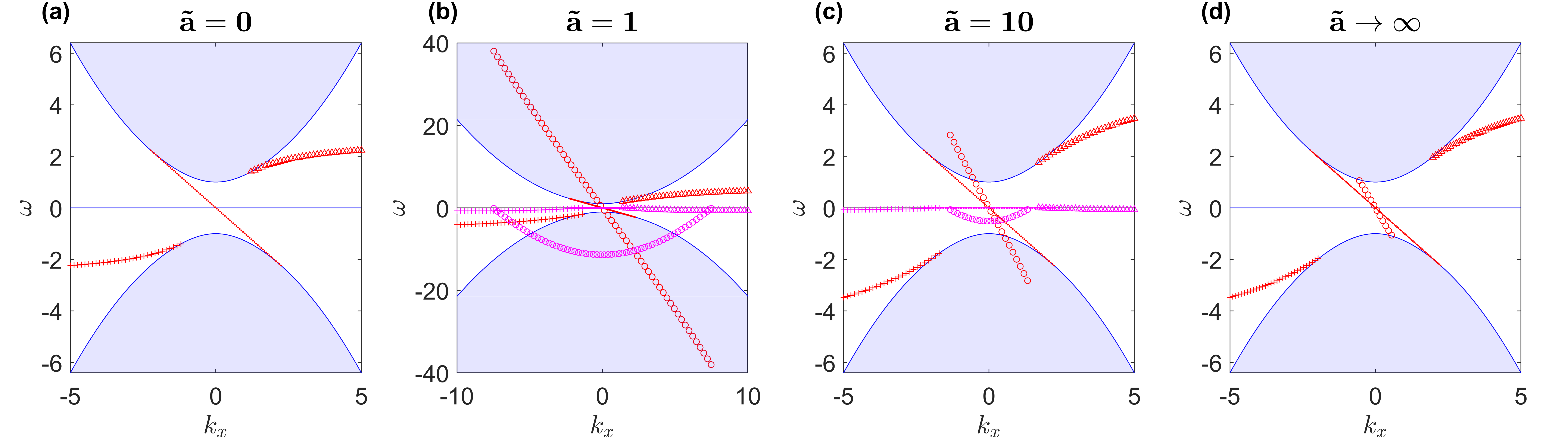
It is easy to check that the Kelvin wave solution $\omega=-k_{x}$ , $v=0$ , still holds in this case, and is independent of $\tilde{a}$ , since $v=0$ means that the boundary condition (37) is reduced to $u|_{y=0}=0$ . Equivalently, we see that the Kelvin wave edge mode obeys both the no-slip condition and the no-stress condition, hence it obeys a linear interpolation between them. Numerically, one finds the other edge modes have complex dispersions with $\mathrm{Im}\left(\omega\right)<0$ , for $\tilde{a}>0$ , meaning that they indeed decay in time (see Fig. 4). This leads to a result unique to the non-Hermitian case — the edge mode dispersions can intersect with the bulk band away from its bottom, since the edge dispersion can “bypass” the bulk dispersion bottom via the imaginary frequency axis.

We briefly describe the dependence of edge mode dispersions on the parameter $\tilde{a}$ (see Fig. 4), with the important point being that there is such a dependence, so the usual BEC is broken, as in the Hermitian case. For $\tilde{a}=0$ (no-slip), there are two edge modes emerging at finite $k_{x}$ and no phase accumulation for $S_{0}$ at infinity; for $\tilde{a}=\infty$ (no-stress), there are three edge modes at finite $k_{x}$ and the appropriate correction at infinity (as seen in Ref. (Tauber et al. 2020)) — these are the Hermitian cases. For any finite $\tilde{a}>0$ , there are three edge modes as well, where two of them emerge not from the bottom of the band. One of them can be continuously related to the mode in the no-slip case, and the other “comes from infinity” — meaning that as $\tilde{a}$ decreases it emerges from the upper band and disappears in the lower band at larger values of $k_{x}$ . For large $\tilde{a}$ , it approaches the third mode in the no-stress case, whose dispersion is almost linear, $\omega\approx-2k_{x}$ ²² 2 In a non-Hermitian system there are in principle other possibilities, such as a residual spectrum, or a point spectrum which covers a 2D domain in the complex plane (Eidelman et al. 2004). By studying the equation $(I\omega-H)\Psi=\Phi$ for arbitrary $\Phi$ one can show these options do not occur, the underlying reason being that the corresponding homogeneous equation always has exactly two modes which decay away from the edge for any $\omega$ away from the bulk spectrum.

III.2 Generalized BEC

As before, we use the scattering state solution (25) with the boundary conditions (37) in order to find the scattering matrix. The structure is the same as before

$\displaystyle S_{\zeta}\left(k_{x},k_{y}\right)$	$\displaystyle=-\frac{\tilde{g}_{\zeta}\left(k_{x},-k_{y}\right)}{\tilde{g}_{\zeta}\left(k_{x},k_{y}\right)},\,\,T_{\zeta}\left(k_{x},k_{y}\right)=-\frac{\tilde{h}_{\zeta}\left(k_{x},k_{y}\right)}{\tilde{g}_{\zeta}\left(k_{x},k_{y}\right)},$
$\displaystyle\tilde{g}_{\zeta}\left(k_{x},k_{y}\right)$	$\displaystyle=\left\|\begin{pmatrix}\left(\tilde{a}\nu ik_{x}-1\right)\hat{u}_{\zeta}\left(k_{x},k_{y}\right)-\tilde{a}\nu ik_{y}\hat{v}_{\zeta}\left(k_{x},k_{y}\right)&\left(\tilde{a}\nu ik_{x}-1\right)\hat{u}_{\infty}\left(k_{x},\kappa_{ev}\right)-\tilde{a}\nu i\kappa_{ev}\hat{v}_{\infty}\left(k_{x},\kappa_{ev}\right)\\ \hat{v}_{\zeta}\left(k_{x},k_{y}\right)&\hat{v}_{\infty}\left(k_{x},\kappa_{ev}\right)\end{pmatrix}\right\|,$
$\displaystyle\tilde{h}_{\zeta}\left(k_{x},k_{y}\right)$	$\displaystyle=\left\|\begin{pmatrix}\left(\tilde{a}\nu ik_{x}-1\right)\hat{u}_{\zeta}\left(k_{x},k_{y}\right)-\tilde{a}\nu ik_{y}\hat{v}_{\zeta}\left(k_{x},k_{y}\right)&\left(\tilde{a}\nu ik_{x}-1\right)\hat{u}_{\infty}\left(k_{x},-k_{y}\right)+\tilde{a}\nu ik_{y}\hat{v}_{\infty}\left(k_{x},-k_{y}\right)\\ \hat{v}_{\zeta}\left(k_{x},k_{y}\right)&\hat{v}_{\infty}\left(k_{x},-k_{y}\right)\end{pmatrix}\right\|.$	(40)

Note that the scattering matrix is no longer unitary. We show analytically in Appendix C that $\left|S_{\zeta}\left(k_{x},k_{y}\right)\right|<1$ for all $k_{y}>0$ , which is the physical half-plane, where the incoming and outgoing waves have the correct propagation direction (towards and away from the boundary, respectively), in accordance with the dissipative nature of the boundary condition (37). Conversely, since the scattering matrix has the property $S_{\zeta}\left(k_{x},-k_{y}\right)=S_{\zeta}^{-1}\left(k_{x},k_{y}\right)$ as before, we see that $\left|S_{\zeta}\left(k_{x},k_{y}\right)\right|>1$ for all $k_{y}<0$ , which is the unphysical half-plane, where the order of incoming and outgoing waves is inverted in the scattering state (25). Specifically, for each complex root $K_{y}>0$ , there is a corresponding pole at $-K_{y}<0$ . These results are supported by our numerical calculations, see Fig. 5.

We now discuss the generalized BEC in the non-Hermitian case. First we review the numerical results shown in Fig. 5, and then use them to motivate our more general claims. We see in the plot of the scattering matrix phase [panels 5(b)–(c)] that the roots and the poles of the scattering matrix are separated, unlike the Hermitian case where they coalesce at $K_{y}=0$ . From Fig. 2, we see that all the roots are in the physical half-plane, $K_{y}>0$ ; this is natural since $|S_{\zeta}(k_{x},k_{y})|<1$ only in that half-plane. However, we still find that the phase accumulated on a contour encircling a root-pole pair is $4\pi$ as before (compare with Fig. 3). Hence, here the root-pole pair has phase of the form of the complex function $\left\{-\left[\bar{z}-\left(K_{x}+iK_{y}\right)\right]/\left[z-\left(K_{x}+iK_{y}\right)\right]\right\}$ , where $z=k_{x}+ik_{y}$ , with non-real $K_{x}+iK_{y}$ , instead of real $K_{x}$ in the Hermitian case. In accordance with these observations, we see [Fig. 5(d)] that in order for the phase of the scattering matrix to count an edge mode merging/emerging at $K_{y}$ , we must take a contour “above” it, i.e., with $k_{y}>K_{y}$ . Indeed, the contour with the smaller $k_{y}$ does not sense the edge mode with $K_{y}>k_{y}$ .

We thus see that the complex dispersion of the edge modes allows intersections with the bulk band away from its bottom. This calls for a way to identify bulk-edge dispersion intersections. For that we will show that the above observations are in fact a special case of a general rule, namely that the bulk-edge dispersion intersections correspond to the roots of the scattering matrix: We use the continuity relations in Eqs. (28) and (29) to write the edge mode ansatz (22) in terms of the bulk eigenmodes, at the mode emergence. Thus, the requirement that this solution obeys the boundary condition (37) results in the equation for the edge dispersion, at the points in the wavevector plane where it coincides with the bulk dispersion (suppressing $k_{x}$ dependence),

\tilde{a}\nu\left(ik_{y}-\mathrm{Im}\left(\kappa_{\mathrm{ev}}\right)\right)\hat{v}_{\infty}\left(\kappa_{\mathrm{ev}}\right)\hat{v}_{\zeta}\left(-k_{y}\right)\\ =\left(ik_{x}\tilde{a}\nu-1\right)\left[\hat{u}_{\infty}\left(\kappa_{\mathrm{ev}}\right)\hat{v}_{\zeta}\left(-k_{y}\right)-\hat{u}_{\zeta}\left(-k_{y}\right)\hat{v}_{\infty}\left(\kappa_{\mathrm{ev}}\right)\right].

(41)

Since the frequency is already set in terms of the other quantities, this is indeed an equation in $k_{x},k_{y}$ . On the other hand, inspection of Eq. (40) yields exactly the same equation upon requiring $S_{\zeta}\left(k_{x},k_{y}\right)=0$ .

Next, we deduce from the above observations that a modification of the relative Levinson’s theorem is required in order for the non-Hermitian generalized BEC to hold. Since the edge mode dispersions intersect with the bulk band at the roots of the scattering matrix, which are separated from its poles, and are thus away from the bottom of the band, we must consider contours with $k_{y}$ large enough. Therefore, in order to count all edge modes, we must take a contour with $k_{y}>\tilde{K}_{y}=\max_{\alpha}\left(K_{y,\alpha}\right)$ , but this comes at a price, that the phase accumulated for modes merging/emerging for all other edge modes (at $K_{y,\alpha}<\tilde{K}_{y}$ ) is smeared [see Fig. 5(d)]. For this reason, the straight line contour must be taken with its edges $k_{x_{1}}\rightarrow-\infty,k_{x_{2}}\rightarrow\infty$ . In practice, for numerical calculations it is enough to use finite $k_{x_{1}},k_{x_{2}}$ which are large enough such that $K_{x,\alpha}$ are all inside of $\left(k_{x_{1}},k_{x_{2}}\right)$ ; For any given $k_{y}>\tilde{K}_{y}$ and any desired resolution $\delta$ , there exist $k_{x_{1}},k_{x_{2}}$ large enough so that $\arg\left[S_{\zeta}\left(k_{x},k_{y}\right)\right]|_{k_{x_{1}}}^{k_{x_{2}}}=2\pi n-\delta$ . We note, similarly to the discussion in Ref. (Graf et al. 2021) Sec. 3.1, that even though the scattering matrix has real roots embedded in the bulk band, it retains its role as the transition matrix between sections, since the contours taken in the $\left(k_{x},k_{y}\right)$ plane avoid these roots, as well as the singularities at $\zeta$ .

We finally arrive at the proof of the non-Hermitian relative Levinson’s theorem (see Sec. I). We use the continuous transition between the Hermitian and non-Hermitian regimes, given by the partial-slip boundary condition (37), as well as the usual argument regarding topological invariants, that the winding of $S_{\zeta}$ , which is an integer, is by continuity constant as a parameter is changed, as long as no roots or singularities of $S_{\zeta}$ cross the contour. We define $b=1/\tilde{a}$ , and start from the no-stress condition at $b=0$ . We then continuously increase $b$ to some value $b_{0}>0$ . We denote by $K_{x}\left(b\right),K_{y}\left(b\right)$ a real root of the scattering matrix $S_{\zeta}\left(k_{x},k_{y}\right)$ for the parameter $b$ of the boundary condition. The continuous change in $b$ causes $K_{y}\left(b\right)$ to continuously increase from $0$ to $K_{y}\left(b_{0}\right)$ , and $K_{x}\left(b\right)$ may move as well. Along this transition, for any value of $b$ we take a straight line contour along $k_{x}\in\left(-\infty,\infty\right)$ , and constant $k_{y}\left(b\right)=K_{y}\left(b\right)+\epsilon$ . For this choice, we see that for any $b\in\left[0,b_{0}\right]$ , the phase of the scattering matrix along the contour counts this edge mode correctly, since the winding of $S_{\zeta}$ is an integer and a continuous function of $k_{x},k_{y},b$ , and the chosen contour avoids the root $K_{y}\left(b\right)$ of $S_{\zeta}$ , as well as its singularity $\zeta$ . Thus, we can use a single contour so that the phase of the scattering matrix counts this edge mode for all $b\in\left[0,b_{0}\right]$ by choosing $k_{y}=K_{y}\left(b_{0}\right)+\epsilon$ . Indeed, still this single contour is a continuous change from the one taken in the Hermitian case for $b=0$ , and thus the winding of $S_{\zeta}$ along the two of them is the same. To complete the proof of the non-Hermitian generalized BEC we note that the same argument is valid for the winding of the scattering matrix along the top of the band, $\mathrm{Ind}\left(S_{\zeta}\left(k_{y}\rightarrow\infty\right)\right)$ . We again start from the no-stress condition at $b=0$ and increase $b$ continuously. There is a straight line contour at large constant $k_{y}$ such that $\mathrm{Ind}\left(S_{\zeta}\left(k_{y}\rightarrow\infty\right)\right)=-1$ (see Fig. 3), which remains constant under the above transition, since it is a continuous function of $b$ . Thus the sum $\mathrm{Ind}(S_{\zeta}(k_{y}\to\infty))+n_{b}$ remains equal to its value at $b=0$ , that is, to the bulk Chern number $C_{+}$ , which is the non-Hermitian generalized BEC, Eq. (2).

A final point relates to the nature of the edge modes at infinity. In Ref. (Graf et al. 2021) it was shown that even when there is no mismatch in the regular BEC, there is an anomaly in Levinson’s theorem at infinity, for the boundary conditions (15). In Appendix D we show a different result for the partial-slip condition (37): While the anomaly appears for any $\tilde{a}>0$ , it vanishes for the no-slip condition, $\tilde{a}=0$ .

IV Large odd viscosity

Here we consider the case of large values of odd viscosity, $f\nu>1/2$ (and comment on the regime $1/4\leq f\nu\leq 1/2$ ). In this case we will see that the minimum of the band dispersion is no longer a single point but rather a circle in the $\left(k_{x},k_{y}\right)$ plane, which will require a modification in the contour we use. More importantly, we will find a region in which there are two propagating bulk solutions at given $\omega,k_{x}$ , hence we will get a $2\times 2$ scattering matrix $S$ , rather than a scalar. First we review the properties of the problem in this regime, which apply to both the Hermitian and non-Hermitian cases, and then we treat each system separately and demonstrate the generalized BEC numerically. We stress that even though the shape of the bulk dispersion is changed, its topology remains as before, namely, by Eq. (31), we have $C_{+}=2$ .

We assume $f,\nu>0$ throughout, and consider first the shape of the bulk dispersion. From Eq. (12), for $f\nu>1/2$ we see that $\omega_{+}\left(\mathbf{k}\right)$ assumes the shape of a Mexican hat, instead of a parabola in the previous case. We note that for $1/4\leq f\nu\leq 1/2$ some calculations are more cumbersome [it is not obvious that $\kappa_{i}\in\mathbb{R}$ , see Eq. (20)] but the results are the same as for $f\nu<1/4$ , as we will briefly explain below. Therefore, for the rest of this section we discuss the regime $f\nu>1/2$ . The minimum of the Mexican hat $\omega_{+}\left(k_{x},k_{y}\right)$ dispersion is then achieved for every point $\left(k_{x},k_{y}\right)$ on the circle (see Ref. (Souslov et al. 2019) for a similar discussion),

k_{x}^{2}+k_{y}^{2}=\frac{2f\nu-1}{2\nu^{2}}\equiv K_{c}^{2}.

(42)

The second important effect comes from the definitions of $\kappa,\kappa_{\mathrm{ev}}$ in Eqs. (20) and (26), for the edge modes and bulk scattering problem, respectively. It turns out that inside the circle (42), the inner root in Eq. (20) is complex, making the solutions $\kappa_{j}$ complex. This appears not to be a problem, since in order for the states in the ansatz (17) to be bound it is sufficient to require $\mathrm{Re}\left(\kappa_{j}\right)>0$ , regardless of the imaginary part. Because every complex number has two square roots which are additive inverses, we can always choose one of them with $\mathrm{Re}\left(\kappa_{j}\right)>0$ , leaving previous calculations of the edge modes intact. For $\kappa_{\mathrm{ev}}$ , appearing in the bulk mode scattering problem, there is a more significant modification. From Eq. (26) we find that $\kappa_{\mathrm{ev}}\in i\mathbb{R}$ if and only if

2k_{x}^{2}+k_{y}^{2}>\frac{2\nu f-1}{\nu^{2}},

(43)

which was trivially satisfied for $f\nu<1/2$ ; as a result, the behavior for $1/4\leq f\nu\leq 1/2$ is similar to $f\nu<1/4$ , as stated above. In contrast, for $f\nu>1/2$ there is an elliptical domain in $\left(k_{x},k_{y}\right)$ ,

2k_{x}^{2}+k_{y}^{2}\leq\frac{2\nu f-1}{\nu^{2}}\equiv K_{e}^{2},

(44)

inside which $\kappa_{\mathrm{ev,div}}$ are real and opposite in sign, i.e., they do not correspond to evanescent/divergent solutions anymore, but rather to propagating waves. Hence, when constructing the superposition state (25), there are four terms: two incoming and two outgoing waves. This requires revising the calculation of the scattering matrix, which is now of dimension $2\times 2$ , and generalizing the definition of its phase. Note that the circle (42) is contained inside the ellipse, with tangent points at $k_{x}=\pm K_{c},k_{y}=0$ .

Let us outline the calculation of the scattering matrix in this case. For clarity we denote in this section $k_{y,1}=k_{y},k_{y,2}=-\kappa_{\mathrm{ev}}\left(k_{y}\right)>0$ , and recall all terms in the scattering state are multiplied by $e^{i(k_{x}x-\omega t)}$ . Note that the circle (42) is the solution to the equation $\left|k_{y,2}\left(k_{y,1}\right)\right|=\left|k_{y,1}\right|$ [see Eq. (26)], and for $k_{y,1}$ outside the circle we find $k_{y,2}\left(k_{y,1}\right)$ inside, and vice versa. We choose a convention for the scattering state based on the case where $k_{y,1}$ is positive and outside the circle (but still inside the ellipse), so as before $e^{-ik_{y,1}y}$ is an incoming wave. Here it is important to note that the dependence of the group velocity on $k_{y}$ is inverted inside the circle (42), so $e^{ik_{y,2}y}$ is an incoming wave for the corresponding $k_{y,2}>0$ inside the circle. Accordingly, we define the full scattering state, for $k_{y,1},k_{y,2}$ in their respective domains, by

\tilde{\psi_{s}}=A\hat{\psi}^{\infty}\left(k_{x},-k_{y,1}\right)e^{-ik_{y,1}y}+B\hat{\psi}^{\infty}\left(k_{x},k_{y,2}\right)e^{ik_{y,2}y}\\ +C\hat{\psi}^{\infty}\left(k_{x},k_{y,1}\right)e^{ik_{y,1}y}+D\hat{\psi}^{\infty}\left(k_{x},-k_{y,2}\right)e^{-ik_{y,2}y},

(45)

where the first two terms are incoming waves. The scattering matrix $S$ is defined by the linear relation between the coefficients of outgoing and incoming terms

\begin{pmatrix}C\\ D\end{pmatrix}=S\begin{pmatrix}A\\ B\end{pmatrix}.

(46)

As usual in scattering problems, by linearity, the simplest way to calculate the matrix elements is to consider each incoming wave separately, and to use the boundary conditions to find how it affects the amplitudes of the two outgoing waves. As the $2\times 2$ matrix form of $S$ is only relevant inside the ellipse, it is sufficient to consider $\hat{\psi}^{\infty}$ [see Eq. (13)], without moving the singularity from infinity. Another conclusion is that one must count separately the edge modes inside the ellipse and outside of it by “gluing” the contours of each domain at the domain edges (see below).

We note that for the above choice $k_{y,1},k_{y,2}$ inside the ellipse are (trivially) continuously related to $k_{y},\kappa_{\mathrm{ev}}$ outside, respectively, with both $k_{y,2},\kappa_{\mathrm{ev}}$ vanishing along the ellipse [see Eq. (26)]. Thus we see that the terms in the first column of $S$ inside the ellipse, namely the terms $S_{11},S_{21}$ , have the same meaning as $S_{\infty},T_{\infty}$ outside [see Eq. (27)], that is, they relate the amplitude of the incoming wave with those of the outgoing and evanescent waves, respectively. Indeed, taking the limits $k_{y,2}\rightarrow 0$ inside and $\kappa_{\mathrm{ev}}\rightarrow 0$ outside leads to

S=\begin{pmatrix}S_{\infty}&0\\ T_{\infty}&-1\end{pmatrix}

(47)

along the ellipse [see Eqs. (49),(52) below for the Hermitian and non-Hermitian cases, respectively]. As a result, we see that $S_{\infty}$ outside the ellipse is continuously related to $\det S$ (whose role will be explained below) inside, up to a minus sign. As in Sec. II.3.1 we can again see continuity relations at the bulk-edge dispersion intersection between $k_{y,1},k_{y,2}$ of the bulk scattering state and $\kappa_{1},\kappa_{2}$ of the edge state ( $j=1,2$ and are interchangeable),

\kappa_{j}=ik_{y,j}.

(48)

We stress that the above form of the scattering wave (45) is not unique, with the particular convention specified above taken for the sake of continuity. A similar choice was made in Sec. II.3.1, where we set $e^{-ik_{y}y}$ as the incoming term in Eq. (25), which fixed $k_{y}>0$ as the physical half-plane, and $k_{y}<0$ as unphysical, namely, that in the unphysical half-plane the scattering matrix relates the incoming waves as dependent on the outgoing waves. This claim is equivalently represented by the property $S_{\infty}\left(-k_{y}\right)=\left(S_{\infty}\left(k_{y}\right)\right)^{-1}$ that we saw above. Similarly, in the current case we conclude that for the given choice in Eq. (45), only the region between the ellipse and the circle with $k_{y}>0$ corresponds to the physical scattering matrix, whereas the other domains inside the ellipse are all unphysical due to the signs of $k_{y,1},k_{y,2}$ , meaning that the outgoing wave precedes the incoming one in at least one of the terms: (i) Positive $k_{y,1}$ inside the circle makes both $e^{-ik_{y,1}y}$ and $e^{ik_{y,2}y}$ outgoing, since $k_{y,2}$ is positive and outside the circle. (ii) Negative $k_{y,1}$ inside the circle makes $e^{ik_{y,2}y}$ outgoing, again since $k_{y,2}$ is positive and outside the circle. (iii) Negative $k_{y,1}$ outside the circle makes $e^{-ik_{y,1}y}$ outgoing. In particular, we get that case (i) above is related to the inverse scattering matrix $S^{-1}$ , since all ingoing and outgoing terms are inverted. Indeed, for both Hermitian and non-Hermitian cases we find the $2\times 2$ scattering matrix satisfies $S\left(-k_{y,1},-k_{y,2}\right)=\left(S\left(k_{y,1},k_{y,2}\right)\right)^{-1}$ [see Eqs. (49),(52) below]. Note that we could have chosen other conventions for the scattering state, for example, to define negative $k_{y,1}$ inside the circle and positive $k_{y,2}$ outside the circle, such that the incoming wave terms would be $e^{-ik_{y,1}y},e^{-ik_{y,2}y}$ . This would of course change the expression for $S$ (and the contours taken below), but not the underlying topological structure.

Returning to our convention (45), the inversion of $S$ when $k_{y,1}$ moves from outside the circle to its inside, is related to the fact that $S$ is defective along the circle. For our scattering state (45) we see that both $k_{y,1}$ and $k_{y,2}$ are positive, so that along the edge of the circle we have $k_{y,2}\left(k_{y,1}\right)=k_{y,1}$ (see above), i.e., the two pairs of incoming and outgoing terms coalesce. As seen in the above discussion, the edge of the circle separates the physical and unphysical domains, as did the $k_{x}$ axis in the small odd viscosity regime. Hence, even though the $2\times 2$ scattering matrix is not well-defined along the edge of the circle, we can still discuss its formal properties there. One such property is $\det S=-1$ along the edge of the circle [see Eqs. (49),(52)], in the same way that $S_{\infty}\left(k_{x},k_{y}=0\right)=-1$ in the small viscosity regime. We also conclude that for both $S_{\infty}$ outside the ellipse and $\det S$ inside, we have singularities at the edges of the ellipse, $k_{x}=\pm K_{c},k_{y}=0$ , since $k_{y,1}=k_{y,2}=0$ inside and similarly $k_{y}=\kappa_{\mathrm{ev}}=0$ outside, so the scattering state is ill-defined.

Regarding the calculation of the phase of $S$ for the relative Levinson’s theorem, the correct expression for the $2\times 2$ scattering matrix is $\arg\left(\det S\right)$ , as hinted in Ref. (Graf and Porta 2013) in Sec. 6.3. There, in the proof of the BEC, the scattering matrix plays the role of the transition matrix, and thus its winding is the first Chern number. For the transition matrix it is known that the winding is given by the winding of the product of its eigenvalues, namely its determinant. In Appendix E we discuss two methods for numerical evaluation of the phase of the scattering matrix, and prove their equivalence, from which the utilization of $\det S$ is also evident.

IV.1 Hermitian edge problem

The results of the calculation in the Hermitian case, with the parameter dependent boundary condition (15), are summarized by

	$\displaystyle S\left(k_{x},k_{y,1}\right)$	$\displaystyle=-\frac{1}{G\left(k_{x},k_{y,1},-k_{y,2}\right)}\begin{pmatrix}G\left(k_{x},-k_{y,1},-k_{y,2}\right)&G\left(k_{x},k_{y,2},-k_{y,2}\right)\\ G\left(k_{x},k_{y,1},-k_{y,1}\right)&G\left(k_{x},k_{y,1},k_{y,2}\right)\end{pmatrix},$
	$\displaystyle G\left(k_{x},k_{y,1},k_{y,2}\right)$	$\displaystyle=\begin{vmatrix}k_{x}\hat{u}_{\infty}\left(k_{x},k_{y,1}\right)+ak_{y,1}\hat{v}_{\infty}\left(k_{x},k_{y,1}\right)&k_{x}\hat{u}_{\infty}\left(k_{x},k_{y,2}\right)+ak_{y,2}\hat{v}_{\infty}\left(k_{x},k_{y,2}\right)\\ \hat{v}_{\infty}\left(k_{x},k_{y,1}\right)&\hat{v}_{\infty}\left(k_{x},k_{y,2}\right)\end{vmatrix},$		(49)

The following properties are immediately found upon inspection

	$\displaystyle G\left(k_{x},k_{y,1},k_{y,2}\right)$	$\displaystyle=-G\left(k_{x},k_{y,2},k_{y,1}\right),$
	$\displaystyle G\left(k_{x},-k_{y,1},-k_{y,2}\right)$	$\displaystyle=-\overline{G\left(k_{x},k_{y,1},k_{y,2}\right)},$		(50)

which together imply the numerators in the off-diagonal terms in $S$ are real. We thus find

\det S=\frac{G\left(k_{x},-k_{y,1},k_{y,2}\right)}{G\left(k_{x},k_{y,1},-k_{y,2}\right)},

(51)

from which, using the above properties, we see that $\left|\det S\right|=1$ , in consistency with the unitarity of $S$ ³³ 3 To be more precise, $S$ as written above is not unitary, but similar to a unitary matrix $\tilde{S}$ by $\tilde{S}=TST^{-1}$ , where $T=\text{diag$\left(1,\sqrt{\left|k_{y,2}/k_{y,1}\right|}\right)$}$ . This is due to the dependence of the amplitude of the eigenmodes (13) on the wavevector $\mathbf{k}$ .

Similarly to the case of small odd viscosity with a Hermitian boundary condition, numerical calculation shows the edge mode dispersions intersect with the bulk at the bottom of the band, which here is the circle (42), with finite $K_{y}$ . Thus, we split the contour to two parts which we glue together: (i) Outside and away from the ellipse we keep the straight line contour along the bottom of the band as before, see Eq. (12). (ii) Inside the ellipse and close to it outside we take the upper half-circle in the clockwise direction, namely $k_{x}^{2}+k_{y}^{2}=K_{c}^{2}+\epsilon$ , with positive $k_{y}$ and small $\epsilon$ . Our numerical results indeed show the phase of $\det S$ accumulated along this path inside the ellipse counts the edge modes according to the relative Levinson’s theorem, see Fig. 6. Furthermore, the proof of the standard (Hermitian) relative Levinson’s theorem follows the same route as in Sec. II.3.2, where we treat $k_{x}$ as a parameter and follow a complex root $K_{y}$ of $S$ as it approaches the real $k_{y}$ axis. The point to note here is that this argument works for the scattering state with two incoming and two outgoing terms (45), since both $k_{y,2},k_{y,1}$ approach the real $k_{y}$ axis together, because of the dependence $k_{y,2}\left(k_{y,1}\right)$ [see Eq. (26)].

To summarize, even though this case requires more cumbersome calculations for the $2\times 2$ scattering matrix, by using $\arg\left(\det S\right)$ instead of $\arg\left(S\right)$ , and a different contour inside the ellipse, the topological structure of the original problem is kept: The number of edge modes changes with the parameter $a$ through four regions as in Sec. II.3.2, and corrected at infinity in the same manner, so that the generalized BEC (34) holds.

IV.2 Non-Hermitian edge problem

In this final case we consider both large odd viscosity, which leads to a $2\times 2$ scattering matrix (49) inside the ellipse (44), and the non-Hermitian partial-slip boundary condition (37), which leads to edge modes decaying in time, $\mathrm{Im}\left(\omega\right)<0$ . The results show the combined effects of these two modifications. We observe the separation of the roots and poles of the scattering matrix ( $\det S$ ) away from the minimum of the band, that is, the circle (42). The dependence on the parameter $\tilde{a}$ remains as in Sec. III — for $\tilde{a}=0$ there are two finite- $k_{x}$ edge modes emerging from the bottom of the bulk band, and for $\tilde{a}>0$ there are three finite- $k_{x}$ edge modes, where the featureless $\omega=-k_{x}$ mode remains as before, whereas the other two modes now emerge outside the circle, that is, away from the bottom of the band. Moreover, the topological structure remains as before, namely the generalized BEC is obeyed with the use of the non-Hermitian relative Levinson’s theorem (1), i.e., we take a contour “above” the roots in order for $\arg\left(\det S\right)$ to count the number of edge-bulk dispersion intersections correctly.

Similarly to the previous case, the calculation of the scattering matrix inside the ellipse (44) results in the form given in Eq. (49), with the difference only in $G$ , which is now given by

\tilde{G}\left(k_{x},k_{y,1},k_{y,2}\right)=\begin{vmatrix}\left(i\tilde{a}\nu k_{x}-1\right)\hat{u}_{\infty}\left(k_{x},k_{y,1}\right)-i\tilde{a}\nu k_{y,1}\hat{v}_{\infty}\left(k_{x},k_{y,1}\right)&\left(i\tilde{a}\nu k_{x}-1\right)\hat{u}_{\infty}\left(k_{x},k_{y,2}\right)-i\tilde{a}\nu k_{y,2}\hat{v}_{\infty}\left(k_{x},k_{y,2}\right)\\ \hat{v}_{\infty}\left(k_{x},k_{y,1}\right)&\hat{v}_{\infty}\left(k_{x},k_{y,2}\right)\end{vmatrix}.

(52)

Direct calculation shows the determinant is of the same form as before [see Eq. (51)], but with $\tilde{G}$ instead of $G$ . Here $\det S$ is not pure phase, and does not have the second property in Eq. (50). In Appendix F we show analytically that $\left|\det S\right|<1$ in the physical domain (inside the ellipse and outside the circle with positive $k_{y,1}$ ), as expected from dissipative (as opposed to gain) boundary conditions. This is supported by our numerical calculations, which further show that $S$ has two distinct eigenvalues $\lambda_{j},j=1,2$ . These obey $\left|\lambda_{j}\right|\leq 1$ in the physical domain, with equality achieved along the circle (42). Hence $S$ is always diagonalizable in our system, even though it is no longer unitary.

Similarly to the case of small odd viscosity in Sec. III.2, we can again see, using the continuity relations (48), that the equation for edge dispersion at these points is exactly the same as requiring $\det S=0$ . Indeed, we see (Fig. 7) that again roots and poles are separated, such that the roots are in the physical domain (outside the circle) and the poles are in the unphysical domain (inside the circle). This is also illustrated in Appendix G.

As in the previous case, we glue two contours: (i) Outside and away from the ellipse a straight line contour along the bottom of the band. (ii) Inside the ellipse and close to it outside, for an edge mode dispersion that intersects the bulk band at $\left(K_{x},K_{y}\right)$ we take $R^{2}=\left(K_{x}\right)^{2}+\left(K_{y}\right)^{2}+\epsilon$ and evaluate $\arg\left(\det S\right)$ along $k_{x}^{2}+k_{y}^{2}=R^{2}$ with $k_{y}>K_{y}>0$ . Our numerical results indeed show the phase of $\det S$ accumulated along this path inside the ellipse counts the edge modes according to the relative Levinson’s theorem, and the winding along the top of the bulk band recovers the generalized BEC, see Fig. 7.

V Discussion and conclusions

In this work we have expanded our understanding of the generalized BEC to the simplest non-Hermitian case, where the bulk problem is Hermitian, and non-Hermiticity arises only from the boundary condition we have introduced. We have seen that the relative Levinson’s theorem can be generalized so as to apply even in this case, while the behavior at infinite wave vector was not affected, allowing us to adjust the generalized BEC to systems with non-Hermitian boundary conditions. We have also allowed large odd viscosity, where the scattering matrix becomes a $2\times 2$ matrix in some parts of the wavevector plane. Upon suitably generalizing the definition of phase of the scattering matrix, we found it also obeys the same form of generalized BEC, even with the non-Hermitian boundary condition.

In future works we intend to use the partial-slip boundary condition together with a non-Hermitian bulk problem, by adding even (dissipative) viscosity as well as friction terms to Eqs. (5). There one can expect exceptional rings to affect the BEC (Zhen et al. 2015; Bergholtz et al. 2021; Souslov et al. 2019). Further down the road we envision taking this model back to the context of solid-state systems, and specifically for edge magnetoplasmons emerging in two-dimensional electron gas under the influence of a magnetic field, where the long-range Coulomb interaction presents the main challenge (Cohen and Goldstein 2018). Another possible route for the future, in order to model more realistic systems, is to take into account the effects of disorder (Burmistrov et al. 2019), on top of non-Hermiticity. The tools developed here may also be relevant to testing the BEC in dissipation-induced topological states (Goldstein 2019; Shavit and Goldstein 2020; Beck and Goldstein 2021). Systems in other topological classes (beyond Chern insulators) (Hasan and Kane 2010; Bansil et al. 2016; Qi and Zhang 2011) would also be interesting to study.

Acknowledgements.

Our work has been supported by the Israel Science Foundation (ISF) and the Directorate for Defense Research and Development (DDR&D) grant No. 3427/21 and by the US-Israel Binational Science Foundation (BSF) Grant No. 2020072.

Appendix A Negative odd viscosity obeys the generalized BEC

The case of $f\nu<0$ obeys the same generalized BEC in both Hermitian and non-Hermitian cases. Assume $f>0,\,\nu<0$ (the case $f<0,\,\nu>0$ has the same topological structure, but with inverted signs). The bulk eigenmodes in Eq. (13) are regular on $\mathbb{R}^{2}\cup\left\{\infty\right\}$ , since $q\rightarrow 1$ for $|\mathbf{k}|\to\infty$ , independently of the angle, which implies trivial bulk topology, in agreement with the bulk topological invariant being $C_{+}=0$ , which was calculated in Refs. (Tauber et al. 2019; Souslov et al. 2019) [see Eq. (31)]. Note that there is no need to move a singularity of the bulk eigenmodes, so $S_{\infty}$ is used for the calculations along the top of the upper band as well.

Similarly to the main text, our numerical calculations give the dependence of the number of finite- $\mathbf{k}$ edge modes emerging from $(+)$ or merging into $(-)$ the upper bulk band on the parameters of the boundary conditions: (i) For the Hermitian boundary condition (15) we find $0,-1,1,0$ edge modes for $a\in\left(-\infty,-\sqrt{2}\right),\left(-\sqrt{2},0\right),\left(0,\sqrt{2}\right),\left(\sqrt{2},\infty\right)$ , respectively. (ii) For the non-Hermitian boundary condition (36) we find $0,-1,-1$ edge modes for $\tilde{a}=0,\tilde{a}\in\left(0,\infty\right),\tilde{a}=\infty$ , respectively. The apparent mismatch with the bulk Chern number $C_{+}$ is amended by the behavior of the scattering matrix at $|\mathbf{k}|\to\infty$ , see Eq. (2). Note that the sign of the term $\mathrm{Ind}\left(S\left(\left|\mathbf{k}\right|\rightarrow\infty\right)\right)$ is inverted here with relation to the case of positive $f,\nu$ , and that the parameter independent Kelvin wave solution, $\omega=-k_{x}$ , $\emph{doesnot}$ occur.

Appendix B Proof of the Hermiticity of the boundary condition (15) and the dissipative nature of the boundary condition (36)

In this appendix we prove that the Hermitian boundary conditions (15) indeed preserve the Hermiticity of the edge problem for any $a\in\mathbb{R}$ (as was already shown in Ref. (Graf et al. 2021), in a less physically-motivated approach), whereas the non-Hermitian partial-slip boundary conditions (36) break Hermiticity for any finite $\tilde{a}$ , and specifically lead to loss and not gain.

Consider $H$ , the Hamiltonian in the main text, Eq. (9) and vectors in the edge problem, $\phi,\psi\in L_{2}\left(\mathbb{R}\times\mathbb{R}_{+}\right)^{\otimes 3}$ , i.e., on the half-plane $\left(x,y\right)\in\mathbb{R}\times\mathbb{R}_{+}$ . Both boundary conditions we consider include the condition

\varphi_{3}|_{y=0}=0,

(53)

and from the definition of the $L_{2}$ space we have the additional assumptions

\lim_{x\rightarrow\pm\infty}\varphi_{i}=\lim_{y\rightarrow+\infty}\varphi_{i}=0,

(54)

for $i=1,2,3$ and for all $\varphi\in L_{2}\left(\mathbb{R}\times\mathbb{R}_{+}\right)^{\otimes 3}$ . We first prove the Hermiticity of the edge problem, namely, $\langle\phi|H|\psi\rangle=\langle\psi|H|\phi\rangle^{*}$ , for the boundary condition (15), for all $a\in\mathbb{R}$ . Direct calculation, using integration by parts and the assumptions (53) and (54), leads to

\langle\phi|H|\psi\rangle=\int_{0}^{\infty}dy\int_{-\infty}^{\infty}dx\left\{\psi_{2}^{*}(-i\partial_{x})\phi_{1}+\psi_{1}^{*}(-i\partial_{x})\phi_{2}+\psi_{3}^{*}(-i\partial_{y})\phi_{1}+\psi_{1}^{*}(-i\partial_{y})\phi_{3}\right.\\ \left.+\psi_{3}^{*}\left[i\left(f+\nu\nabla^{2}\right)\right]\phi_{2}+\psi_{2}^{*}\left[-i\left(f+\nu\nabla^{2}\right)\right]\phi_{3}\right\}^{*}-i\nu\int_{-\infty}^{\infty}dx\left[\phi_{2}^{*}\partial_{y}\psi_{3}+\psi_{2}\partial_{y}\phi_{3}^{*}\right]_{y=0}^{\infty}\\ =\langle\psi|H|\phi\rangle^{*}+i\nu\int_{-\infty}^{\infty}dx\left(\phi_{2}^{*}\partial_{y}\psi_{3}+\psi_{2}\partial_{y}\phi_{3}^{*}\right)|_{y=0},

(55)

where specifically the boundary terms resulting from the density gradient (e.g. $\phi_{2}^{*}\partial_{x}\psi_{1}$ ) and Coriolis (e.g. $\phi_{2}^{*}f\psi_{3}$ ) vanish. Since the boundary condition (15) implies $\partial_{y}\varphi_{3}=-a^{-1}\partial_{x}\varphi_{2}$ , the remaining boundary term, related to the odd viscosity, vanishes as well

i\nu\int_{-\infty}^{\infty}dx\left(\phi_{2}^{*}\partial_{y}\psi_{3}+\psi_{2}\partial_{y}\phi_{3}^{*}\right)|_{y=0}\\ =-i\frac{\nu}{a}\int_{-\infty}^{\infty}dx\left(\phi_{2}^{*}\partial_{x}\psi_{2}+\psi_{2}\partial_{x}\phi_{2}^{*}\right)|_{y=0}\\ =-i\frac{\nu}{a}\int_{-\infty}^{\infty}dx\partial_{x}\left(\phi_{2}^{*}\psi_{2}\right)|_{y=0}=0.

(56)

So indeed $\langle\phi|H|\psi\rangle=\langle\psi|H|\phi\rangle^{*}$ for all $a\in\mathbb{R}$ . Recall that $a=-1$ is the no-stress condition, so we have proved its Hermiticity along the way as well. Furthermore, we note that the above calculation also shows that the no-slip condition ( $\varphi_{2}|_{y=0}=0$ ) leads to a Hermitian edge problem, since the last term in Eq. (55) vanishes trivially.

For the partial-slip boundary conditions (36) with $\tilde{a}>0$ , we consider the expectation value, $\langle\psi|H_{1}|\psi\rangle$ , of the operator $H_{1}=\left(H-H^{\dagger}\right)/2i=\mathrm{Im}\left(H\right)$ , and show that it is strictly non-positive, which implies that the operator $H_{1}$ is negative-semidefinite. In fact, we will show that the edge frequency eigenvalues of $H$ have negative imaginary part, $\mathrm{Im}\left(\omega\right)<0$ , which leads to edge modes decaying in time (except for the boundary-condition independent $\omega=-k_{x}$ edge mode, for which $v=0$ everywhere so the second term in Eq. (55) vanishes, which means it is Hermitian). Thus, the edge problem with the partial-slip boundary conditions has strictly non-real spectrum, so it is non-Hermitian. Again using the assumptions (53),(54), we see that the density gradient and Coriolis terms do not contribute to the expectation value $\langle\psi|H_{1}|\psi\rangle$ , since all the corresponding boundary terms vanish upon using integration by parts. Hence, we may focus solely on the terms involving odd viscosity. The viscous terms appear in the Hamiltonian as $\left(H\mathbf{v}\right)_{a}=-i\left(\nabla\cdot T\right)_{a}$ , with $\mathbf{v}=\left(u,v\right)^{T}$ , so we may write (employing Einstein summation)

\langle\psi|H_{1}|\psi\rangle=\mathrm{Im}\left(\langle\psi|H|\psi\rangle\right)\\ =\mathrm{Im}\left(-i\int_{0}^{\infty}dy\int_{-\infty}^{\infty}dxv_{a}^{*}\partial_{b}T_{ab}\right)\\ =-\mathrm{Re}\left(\int_{0}^{\infty}dy\int_{-\infty}^{\infty}dxv_{a}^{*}\partial_{b}T_{ab}\right).

(57)

Using integration by parts and the assumptions above, we find

\langle\psi|H_{1}|\psi\rangle=\mathrm{Re}\left[\int_{0}^{\infty}dy\int_{-\infty}^{\infty}dx\left(\partial_{b}v_{a}^{*}\right)T_{ab}\right]\\ +\mathrm{Re}\left[\int_{-\infty}^{\infty}\left(u^{*}T_{xy}\right)|_{y=0}dx\right].

(58)

The first term in the above expression vanishes, since we only consider odd viscosity: Substituting $T_{ab}=-\nu_{abcd}^{-}\partial_{d}v_{c}$ , we observe that

\mathrm{Re}\left[\int_{0}^{\infty}dy\int_{-\infty}^{\infty}dx\left(\partial_{b}v_{a}^{*}\right)T_{ab}\right]\\ =-\mathrm{Re}\left[\int_{0}^{\infty}dy\int_{-\infty}^{\infty}dx\nu_{abcd}^{-}\left(\partial_{b}v_{a}^{*}\right)\left(\partial_{d}v_{c}\right)\right],

(59)

and note that the term $\nu_{abcd}^{-}\left(\partial_{b}v_{a}^{*}\right)\left(\partial_{d}v_{c}\right)$ is pure imaginary, since, by definition, the odd part satisfies $\nu_{abcd}^{-}=-\nu_{cdab}^{-}$ (Avron 1998). For any $\tilde{a}>0$ , we plug in the boundary condition (36), $u|_{y=0}=-\tilde{a}T_{xy}|_{y=0}$ , and find that the second term in Eq. (58) is indeed negative

\langle\psi|H_{1}|\psi\rangle=-\frac{1}{\tilde{a}}\mathrm{Re}\left[\int_{-\infty}^{\infty}\left(u^{*}u\right)|_{y=0}dx\right]<0.

(60)

Thus, as expected in the main text, $\tilde{a}>0$ leads to dissipation of all edge modes [except for the $\omega=-k_{x}$ one, for which $u=0$ at the edge for all $\tilde{a}$ , see Eq. (37)], while $\tilde{a}<0$ would be unphysical, as it leads to gain ( $\mathrm{Im}\left(\omega\right)>0$ ) in the edge problem. We briefly note that the Hermitian boundary conditions obey $\langle\psi|H_{1}|\psi\rangle=0$ , but of course this is not enough to prove Hermiticity, since non-Hermitian operators may have strictly real spectrum as well, hence above we resorted to a direct proof of Hermiticity.

Appendix C The scattering matrix decreases amplitudes in the non-Hermitian case

In this appendix we show that for a $1\times 1$ scattering matrix, $\left|S_{\zeta}\left(k_{x},k_{y}\right)\right|<1$ for $k_{y}>0$ , which corresponds to the boundary condition (37) causing dissipation (i.e., loss rather than gain), in the domain where it is well-defined in terms of direction of wave propagation. Note that here, as in the Hermitian case, moving the singularity does not affect the absolute value of the scattering matrix, since

S_{\zeta}\left(k_{x},k_{y}\right)=\frac{t_{\infty}^{\zeta}\left(k_{x},-k_{y}\right)}{t_{\infty}^{\zeta}\left(k_{x},k_{y}\right)}S_{\infty}\left(k_{x},k_{y}\right).

(61)

Since, by Eq. (14), $\left|t_{\infty}^{\zeta}\left(k_{x},k_{y}\right)\right|=1$ , it is indeed enough to consider $S_{\infty}$ . By continuity, it is enough to show that $\left|S_{\infty}\right|=1$ if and only if $k_{y}=0$ , using the fact that we have seen the roots (where $\left|S_{\infty}\right|=0<1$ ) are in $k_{y}>0$ . One direction is trivial: plug $k_{y}=0$ and see $S_{\infty}=-1$ . For the other direction, we write the equation

\left|S_{\infty}\right|^{2}=1,

(62)

and assume $k_{y}\neq 0$ . We expand using Eq. (40) and the definitions of the bulk modes (13) to find

0=\nu\omega_{+}\mathrm{Im}\left(\kappa_{\mathrm{ev}}\right)\mathbf{k}^{2}\left(2\mathbf{k}^{2}+\frac{1-2f\nu}{\nu^{2}}\right)+\\ +k_{x}\mathbf{k}^{2}\left[2\nu^{2}\mathbf{k}^{4}+\mathbf{k}^{2}\left(3-4f\nu\right)\right.\\ \left.+\left(-\frac{f}{\nu}+\frac{1}{\nu^{2}}\left(1-2f\nu\right)+2f^{2}\right)\right].

(63)

Working under the assumption that $f\nu<1/4$ we see that the first term is strictly positive. The second term vanishes only at

\mathbf{k}_{\pm}^{2}=\frac{1}{\nu^{2}}\left(f\nu+\frac{-3\pm 1}{4}\right)<0,

(64)

so it is strictly positive as well. Therefore, for any $\mathbf{k}^{2}\neq 0$ , the entire RHS in Eq. (63) is positive, and indeed there are no other solutions to the equation.

Appendix D The anomaly of Levinson’s theorem at infinity for the non-Hermitian case

Similarly to Sec. 3.5 of Ref. (Graf et al. 2021), we expand $S_{0}$ [Eq. (40)] in the non-Hermitian case at $\left|\mathbf{k}\right|\rightarrow\infty$ , and show an anomaly of Levinson’s theorem occurs for all $\tilde{a}>0$ but not for the no-slip condition, $\tilde{a}=0$ . Even though the anomaly is absent from the $\tilde{a}=0$ case, we find the winding of $S_{0}$ at infinity to be in agreement with our numerical results in the main text.

First, we briefly explain the anomaly as presented in Ref. (Graf et al. 2021). There it is shown for the family of boundary conditions (15), that the winding of the scattering matrix along the top of the upper bulk band, corresponds to no edge mode at $\left|\mathbf{k}\right|\rightarrow\infty$ . More explicitly, this means that for $\left|a\right|<\sqrt{2}$ , where the BEC is amended by the winding of the scattering matrix along the top of the band, there are no edge modes at $\left|\mathbf{k}\right|\rightarrow\infty$ , in the sense that there are no poles of $S_{0}$ there. The opposite is true for $\left|a\right|>\sqrt{2}$ , namely, while the edge index of the finite- $\mathbf{k}$ edge modes matches the Chern number, and accordingly there is no winding of the scattering matrix at $\left|\mathbf{k}\right|\rightarrow\infty$ , there are edge modes there (poles of $S_{0}$ ). We will now show that with the non-Hermitian boundary conditions (37), similar behavior occurs for $\tilde{a}>0$ , where $S_{0}$ winds at infinity and there are no edge modes there, but not for $\tilde{a}=0$ , where there are neither winding nor edge modes.

For the non-Hermitian boundary condition (37), we expand $g_{0}\left(k_{x},-k_{y}\right)$ [see Eq. (40)] at $\left|\mathbf{k}\right|\rightarrow\infty$ and find

g_{0}\left(k_{x},-k_{y}\right)\sim\frac{i}{2}\left[\tilde{a}\nu\left(2ik_{x}+k_{y}+\kappa_{\mathrm{ev}}\right)-2\right],

(65)

\arg\left(S_{0}\right)=2\arg\left(g_{0}\left(k_{x},-k_{y}\right)\right),

(66)

and from Eq. (26),

\kappa_{\mathrm{ev}}\sim i\sqrt{2k_{x}^{2}+k_{y}^{2}}.

(67)

For $\tilde{a}>0$ the leading order expansion is thus

g_{0}\left(k_{x},-k_{y}\right)\sim\frac{i}{2}\left[\tilde{a}\nu\left(2ik_{x}+k_{y}+\kappa_{\mathrm{ev}}\right)\right].

(68)

Next, we take the reciprocal coordinates

k_{x}=\frac{\lambda_{x}}{\lambda_{x}^{2}+\lambda_{y}^{2}},k_{y}=\frac{\lambda_{y}}{\lambda_{x}^{2}+\lambda_{y}^{2}},

(69)

which exchange $0$ and $\infty$ , and thus, using Eq. (67), we get

g_{0}\left(k_{x},-k_{y}\right)\sim-\frac{\tilde{a}\nu}{2\left(\lambda_{x}^{2}+\lambda_{y}^{2}\right)}\left(2\lambda_{x}+\sqrt{2\lambda_{x}^{2}+\lambda_{y}^{2}}-i\lambda_{y}\right).

(70)

From this expression we now show that $S_{0}$ does wind at $\left|\mathbf{k}\right|\rightarrow\infty$ , and yet, there are no roots of $S_{0}$ there. For the calculation of the winding of $S_{0}$ , the prefactor in Eq. (70) is irrelevant, while the last term, $-i\lambda_{y}$ , determines that the phase will be accumulated from below the real line. Futhermore, for any (small) constant $k_{y}>0$ we have

\lim_{\lambda_{x}\rightarrow\pm\infty}2\lambda_{x}+\sqrt{2\lambda_{x}^{2}+\lambda_{y}^{2}}=\pm\infty.

(71)

We note that in the parametrization Eq. (69), $\lambda_{x}$ traverses the real line in the opposite direction to $k_{x}$ . Therefore, as $k_{x}$ varies from $-\infty$ to $\infty$ , the phase $\arg\left(g_{0}\left(k_{x},-k_{y}\right)\right)$ is changed from from $0$ to $-\pi$ . Finally, with (66) we obtain $\Delta\left[\arg\left(S_{0}\right)\right]=-2\pi$ , i.e., $\mathrm{Ind}\left(S_{0}\left(k_{y}\rightarrow\infty\right)\right)=-1$ , as expected from the numerical results presented in the main text, see Fig. 5.

For the roots of $S_{0}$ , we again use the expansions (68) and (67), along with the expansion of Eq. (12)

\omega\sim\nu\left(k_{x}^{2}+k_{y}^{2}\right)\sim\nu\left(k_{x}^{2}+\kappa_{\mathrm{ev}}^{2}\right).

(72)

Since $g_{0}$ is homogeneous in $k_{x},k_{y}$ [see Eq. (68)], we may use the ansatz

k_{y}=ic_{+}k_{x},\,\kappa_{\mathrm{ev}}=-ic_{-}k_{x}.

(73)

Thus, from requiring $g_{0}=0$ we have the equation

2+c_{+}-c_{-}=0,

(74)

while from Eq. (67) we have the constraint

c_{+}^{2}+c_{-}^{2}=2.

(75)

Their only joint solution is $c_{+}=-1,c_{-}=1$ , but this is not a valid solution, since plugging it into Eq. (72) leads to $\omega=0$ , which is not in the upper bulk band. So again, as expected, there is no root of $S_{0}$ at $\left|\mathbf{k}\right|\rightarrow\infty$ .

Finally we consider the expansion of $g_{0}$ for $\tilde{a}=0$ . From (65) we see that $g_{0}\sim-i$ to leading order. Thus, there is no winding of $S_{0}$ , and also no roots of $S_{0}$ , in contrast to the previous case. We note that higher orders in the expansion will have lower powers of $\mathbf{k}$ , so they cannot add roots.

Appendix E Equivalence of numerical methods for evaluation of the phase of the scattering matrix

We briefly introduce the two methods for numerical calculation of the phase of the scattering matrix, which apply to both matrix and scalar $S$ for both the Hermitian and non-Hermitian cases, and prove they are equivalent. The first method is to evaluate directly the phase of the complex number $\varphi=\arg\left(\det S\right)$ . This method is straightforward, but when the phase winds over more than one $2\pi$ cycle, one must “unwrap” the phase accordingly. The second option is to numerically integrate over $d\varphi=\mathrm{Im}\left(\mathrm{Tr}\left(S^{-1}dS\right)\right)$ , which by nature results in relative phase, and thus its value depends on the starting point. Since we are interested in the phase difference accumulated along some finite contour, this is not a problem.

Let us show in a general framework why these two methods are equivalent: For all matrices it is known that $\ln\left(\det S\right)=\mathrm{Tr}\left(\ln S\right)$ . Also, for every complex number $\arg\left(z\right)=\mathrm{Im}\left(\ln\left(z\right)\right)$ (assuming main branch). We now define the phase of a matrix $S$ to be $\varphi=\mathrm{Im}\left(\mathrm{Tr}\left(\ln S\right)\right)$ , so $\varphi=\mathrm{Im}\left(\ln\left(\det S\right)\right)=\arg\left(\det S\right)$ . On the other hand, $d\varphi=\mathrm{Im}\left(\mathrm{Tr}\left(d\left(\ln S\right)\right)\right)\overset{(*)}{=}\mathrm{Im}\left(\mathrm{Tr}\left(S^{-1}dS\right)\right)$ , with $(*)$ relying on the cyclic property of the trace. Thus we get $\arg\left(\det S\right)=\int\mathrm{Im}\left(\mathrm{Tr}\left(S^{-1}dS\right)\right)$ , as wanted. Note that this is true even if $S$ does not commute with itself at different points along the integration contour, and even if $S$ is not unitary (which is especially important in the non-Hermitian case).

Appendix F The scattering matrix decreases amplitudes in the non-Hermitian case with large odd viscosity

Similar to the calculation in Appendix C, we now show that $\left|\det S\right|<1$ for $k_{y}>0$ inside the ellipse (44) and outside the circle (42), for the $2\times 2$ scattering matrix in the non-Hermitian case. It is enough from continuity to show that $\left|\det S\right|=1$ if and only if $k_{y,1}=k_{y,2}$ , since the solution to the equation $k_{y,2}\left(k_{y,1}\right)=k_{y,1}$ is exactly the circle, and we have shown above that the roots (where $\left|\det S\right|=0<1$ ) are outside the circle. As before, one direction is trivial — plugging $k_{y,1}=k_{y,2}$ into Eqs. (51),(52) yields $\det S=-1$ . For the other direction we expand the equation

\left|\det S\right|^{2}=1

(76)

to find

0=-\left(1-\frac{k_{x}^{2}}{\omega^{2}}\right)\tilde{a}\nu\left(k_{y,1}+k_{y,2}\right)\left(q\left(k_{y,2}\right)-q\left(k_{y,1}\right)\right).

(77)

Using Eq. (13) we see

q\left(k_{y,2}\right)-q\left(k_{y,1}\right)=\frac{\nu}{\omega}\left(k_{y,1}^{2}-k_{y,2}^{2}\right),

(78)

so indeed the equation

0=-\left(1-\frac{k_{x}^{2}}{\omega^{2}}\right)\tilde{a}\nu\left(k_{y,1}+k_{y,2}\right)^{2}\frac{\nu}{\omega}\left(k_{y,1}-k_{y,2}\right)

(79)

has a single solution $k_{y,1}=k_{y,2}$ (and $\omega=-k_{x}$ which is irrelevant for a scattering state solution).

Appendix G $\left|\det S\right|$ in the non-Hermitian case with large odd viscosity

In Fig. 8, by plotting $\left|\det S\right|$ , we show that the roots of $\det S$ are in the physical domain, namely outside the circle (42) and inside the ellipse (44), in the upper half-plane, and the poles are in the unphysical domain, inside the upper half of the circle. As mentioned in the main text, in the Hermitian case the root and pole coalesce at the edge of the circle, which is the bottom of the bulk band, while in the non-Hermitian case they are separated along the edge of the circle, as the imaginary part of the edge dispersion allows them to emerge away from the bottom of the bulk band.

Let us note that the hill on the negative part of the $k_{y}$ axis, seen in Fig. 8, has a finite height, and is thus not a pole for the shown parameters. For other values of $\tilde{a}$ there are two poles in the unphysical domain, one inside the circle and one outside, both with negative $k_{y}$ along the $k_{y}$ axis. They do not correspond to roots or poles in the physical domain, and thus bear no physical meaning.

References

Hasan and Kane (2010) M. Z. Hasan and C. L. Kane, Colloquium: Topological insulators, Rev. Mod. Phys. 82, 3045 (2010).
Bansil et al. (2016) A. Bansil, H. Lin, and T. Das, Colloquium: Topological band theory, Rev. Mod. Phys. 88, 021004 (2016).
Qi and Zhang (2011) X. L. Qi and S. C. Zhang, Topological insulators and superconductors, Rev. Mod. Phys. 83, 1057 (2011).
Haldane (1988) F. D. M. Haldane, Model for a Quantum Hall Effect without Landau Levels: Condensed-Matter Realization of the "Parity Anomaly", Phys. Rev. Lett. 61, 2015 (1988).
Khanikaev et al. (2013) A. B. Khanikaev, S. Hossein Mousavi, W. K. Tse, M. Kargarian, A. H. MacDonald, and G. Shvets, Photonic topological insulators, Nat. Mater. 12, 233 (2013).
Lu et al. (2014) L. Lu, J. D. Joannopoulos, and M. Soljačić, Topological photonics, Nat. Photonics 8, 821 (2014).
Ozawa et al. (2019) T. Ozawa, H. M. Price, A. Amo, N. Goldman, M. Hafezi, L. Lu, M. C. Rechtsman, D. Schuster, J. Simon, O. Zilberberg, and I. Carusotto, Topological photonics, Rev. Mod. Phys. 91, 015006 (2019).
Harari et al. (2018) G. Harari, M. A. Bandres, Y. Lumer, M. C. Rechtsman, Y. D. Chong, M. Khajavikhan, D. N. Christodoulides, and M. Segev, Topological insulator laser: Theory, Science 359, eaar4003 (2018).
Bandres et al. (2018) M. A. Bandres, S. Wittek, G. Harari, M. Parto, J. Ren, M. Segev, D. N. Christodoulides, and M. Khajavikhan, Topological insulator laser: Experiments, Science 359, eaar4005 (2018).
Xin et al. (2020) L. Xin, Y. Siyuan, L. Harry, L. Minghui, and C. Yanfeng, Topological mechanical metamaterials: A brief review, Curr. Opin. Solid State Mater. Sci. 24, 100853 (2020).
Ma et al. (2019) G. Ma, M. Xiao, and C. T. Chan, Topological phases in acoustic and mechanical systems, Nat. Rev. Phys. 1, 281 (2019).
Zhang et al. (2018) X. Zhang, M. Xiao, Y. Cheng, M.-H. Lu, and J. Christensen, Topological sound, Commun. Phys. 1, 97 (2018).
Kane and Lubensky (2014) C. L. Kane and T. C. Lubensky, Topological boundary modes in isostatic lattices, Nat. Phys. 10, 39 (2014).
Prodan and Prodan (2009) E. Prodan and C. Prodan, Topological Phonon Modes and Their Role in Dynamic Instability of Microtubules, Phys. Rev. Lett. 103, 248101 (2009).
He et al. (2016) C. He, X. Ni, H. Ge, X.-C. Sun, Y.-B. Chen, M.-H. Lu, X.-P. Liu, and Y.-F. Chen, Acoustic topological insulator and robust one-way sound transport, Nat. Phys. 12, 1124 (2016).
Lee et al. (2018) C. H. Lee, S. Imhof, C. Berger, F. Bayer, J. Brehm, L. W. Molenkamp, T. Kiessling, and R. Thomale, Topolectrical Circuits, Commun. Phys. 1, 39 (2018).
Shankar et al. (2022) S. Shankar, A. Souslov, M. J. Bowick, M. C. Marchetti, and V. Vitelli, Topological active matter, Nat. Rev. Phys. 4, 380 (2022).
Shankar et al. (2017) S. Shankar, M. J. Bowick, and M. C. Marchetti, Topological Sound and Flocking on Curved Surfaces, Phys. Rev. X 7, 031039 (2017).
Souslov et al. (2017) A. Souslov, B. C. van Zuiden, D. Bartolo, and V. Vitelli, Topological sound in active-liquid metamaterials, Nat. Phys. 13, 1091 (2017).
Souslov et al. (2019) A. Souslov, K. Dasbiswas, M. Fruchart, S. Vaikuntanathan, and V. Vitelli, Topological Waves in Fluids with Odd Viscosity, Phys. Rev. Lett. 122, 128001 (2019).
Thouless et al. (1982) D. J. Thouless, M. Kohmoto, M. P. Nightingale, and M. den Nijs, Quantized Hall Conductance in a Two-Dimensional Periodic Potential, Phys. Rev. Lett. 49, 405 (1982).
Hatsugai (1993a) Y. Hatsugai, Edge states in the integer quantum Hall effect and the Riemann surface of the Bloch function, Phys. Rev. B 48, 11851 (1993a).
Hatsugai (1993b) Y. Hatsugai, Chern number and edge states in the integer quantum Hall effect, Phys. Rev. Lett. 71, 3697 (1993b).
Bal (2019) G. Bal, Continuous bulk and interface description of topological insulators, J. Math. Phys. 60, 081506 (2019).
Tauber et al. (2019) C. Tauber, P. Delplace, and A. Venaille, A bulk-interface correspondence for equatorial waves, J. Fluid Mech. 868, R2 (2019).
Tauber et al. (2020) C. Tauber, P. Delplace, and A. Venaille, Anomalous bulk-edge correspondence in continuous media, Phys. Rev. Res. 2, 013147 (2020).
Silveirinha (2019) M. G. Silveirinha, Proof of the Bulk-Edge Correspondence through a Link between Topological Photonics and Fluctuation-Electrodynamics, Phys. Rev. X 9, 011037 (2019).
Van Mechelen and Jacob (2018) T. Van Mechelen and Z. Jacob, Quantum gyroelectric effect: Photon spin-1 quantization in continuum topological bosonic phases, Phys. Rev. A 98, 023842 (2018).
Van Mechelen et al. (2021) T. Van Mechelen, W. Sun, and Z. Jacob, Optical N-invariant of graphene’s topological viscous Hall fluid, Nat. Commun. 12, 4729 (2021).
Graf et al. (2021) G. M. Graf, H. Jud, and C. Tauber, Topology in Shallow-Water Waves: A Violation of Bulk-Edge Correspondence, Commun. Math. Phys. 383, 731 (2021).
Rotter (2009) I. Rotter, A non-Hermitian Hamilton operator and the physics of open quantum systems, J. Phys. A Math. Theor. 42, 153001 (2009).
Yokomizo and Murakami (2019) K. Yokomizo and S. Murakami, Non-Bloch Band Theory of Non-Hermitian Systems, Phys. Rev. Lett. 123, 066404 (2019).
Ashida et al. (2020) Y. Ashida, Z. Gong, and M. Ueda, Non-Hermitian physics, Adv. Phys. 69, 249 (2020).
Bender (2007) C. M. Bender, Making sense of non-Hermitian Hamiltonians, Reports Prog. Phys. 70, 947 (2007).
Bergholtz et al. (2021) E. J. Bergholtz, J. C. Budich, and F. K. Kunst, Exceptional topology of non-Hermitian systems, Rev. Mod. Phys. 93, 015005 (2021).
Shen et al. (2018) H. Shen, B. Zhen, and L. Fu, Topological Band Theory for Non-Hermitian Hamiltonians, Phys. Rev. Lett. 120, 146402 (2018).
Gong et al. (2018) Z. Gong, Y. Ashida, K. Kawabata, K. Takasan, S. Higashikawa, and M. Ueda, Topological Phases of Non-Hermitian Systems, Phys. Rev. X 8, 031079 (2018).
Esaki et al. (2011) K. Esaki, M. Sato, K. Hasebe, and M. Kohmoto, Edge states and topological phases in non-Hermitian systems, Phys. Rev. B 84, 205128 (2011).
Kunst et al. (2018) F. K. Kunst, E. Edvardsson, J. C. Budich, and E. J. Bergholtz, Biorthogonal Bulk-Boundary Correspondence in Non-Hermitian Systems, Phys. Rev. Lett. 121, 026808 (2018).
Lee (2016) T. E. Lee, Anomalous Edge State in a Non-Hermitian Lattice, Phys. Rev. Lett. 116, 133903 (2016).
Martinez Alvarez et al. (2018) V. M. Martinez Alvarez, J. E. Barrios Vargas, and L. E. F. Foa Torres, Non-Hermitian robust edge states in one dimension: Anomalous localization and eigenspace condensation at exceptional points, Phys. Rev. B 97, 121401(R) (2018).
Yao and Wang (2018) S. Yao and Z. Wang, Edge States and Topological Invariants of Non-Hermitian Systems, Phys. Rev. Lett. 121, 086803 (2018).
Yokomizo and Murakami (2020) K. Yokomizo and S. Murakami, Non-Bloch band theory and bulk-edge correspondence in non-Hermitian systems, Prog. Theor. Exp. Phys. 2020, 12 (2020).
Xiong (2018) Y. Xiong, Why does bulk boundary correspondence fail in some non-hermitian topological models, J. Phys. Commun. 2, 035043 (2018).
Leykam et al. (2017) D. Leykam, K. Y. Bliokh, C. Huang, Y. D. Chong, and F. Nori, Edge Modes, Degeneracies, and Topological Numbers in Non-Hermitian Systems, Phys. Rev. Lett. 118, 040401 (2017).
Kunst and Dwivedi (2019) F. K. Kunst and V. Dwivedi, Non-Hermitian systems and topology: A transfer-matrix perspective, Phys. Rev. B 99, 245116 (2019).
Lee and Thomale (2019) C. H. Lee and R. Thomale, Anatomy of skin modes and topology in non-Hermitian systems, Phys. Rev. B 99, 201103(R) (2019).
Imura and Takane (2019) K.-I. Imura and Y. Takane, Generalized bulk-edge correspondence for non-Hermitian topological systems, Phys. Rev. B 100, 165430 (2019).
Longhi (2021) S. Longhi, Bulk-edge correspondence and trapping at a non-Hermitian topological interface, Opt. Lett. 46, 6107 (2021).
Vallis (2017) G. K. Vallis, Atmospheric and Oceanic Fluid Dynamics (Cambridge University Press, Cambridge, UK, 2017) pp. 1–946.
Cohen and Goldstein (2018) R. Cohen and M. Goldstein, Hall and dissipative viscosity effects on edge magnetoplasmons, Phys. Rev. B 98, 235103 (2018).
Graf and Porta (2013) G. M. Graf and M. Porta, Bulk-Edge Correspondence for Two-Dimensional Topological Insulators, Commun. Math. Phys. 324, 851 (2013).
(53) A different approach has recently been presented in Ref. (Tauber and Thiang 2023). There the spectral flow of the edge modes as a function of an appropriate parametrization of the family of boundary conditions (15) was considered, leading to a BEC which in a sense averages over this family. However, in many situations a fixed boundary condition is considered, with no straightforward generalization to an appropriate family, in particular non-Hermitian ones. Hence we prefer to study fixed boundary conditions in the non-Hermitian case.
Avron (1998) J. E. Avron, Odd viscosity, J. Stat. Phys. 92, 543 (1998).
Avron et al. (1995) J. E. Avron, R. Seiler, and P. G. Zograf, Viscosity of Quantum Hall Fluids, Phys. Rev. Lett. 75, 697 (1995).
Bradlyn et al. (2012) B. Bradlyn, M. Goldstein, and N. Read, Kubo formulas for viscosity: Hall viscosity, Ward identities, and the relation with conductivity, Phys. Rev. B 86, 245309 (2012).
Maxwell (1879) J. C. Maxwell, VII. On stresses in rarified gases arising from inequalities of temperature, Philos. Trans. R. Soc. London 170, 231 (1879).
Torre et al. (2015) I. Torre, A. Tomadin, A. K. Geim, and M. Polini, Nonlocal transport and the hydrodynamic shear viscosity in graphene, Phys. Rev. B 92, 165433 (2015).
Falkovich and Levitov (2017) G. Falkovich and L. Levitov, Linking Spatial Distributions of Potential and Current in Viscous Electronics, Phys. Rev. Lett. 119, 066601 (2017).
Kiselev and Schmalian (2019) E. I. Kiselev and J. Schmalian, Boundary conditions of viscous electron flow, Phys. Rev. B 99, 035430 (2019).
(61) In a non-Hermitian system there are in principle other possibilities, such as a residual spectrum, or a point spectrum which covers a 2D domain in the complex plane (Eidelman et al. 2004). By studying the equation $(I\omega-H)\Psi=\Phi$ for arbitrary $\Phi$ one can show these options do not occur, the underlying reason being that the corresponding homogeneous equation always has exactly two modes which decay away from the edge for any $\omega$ away from the bulk spectrum.
(62) To be more precise, $S$ as written above is not unitary, but similar to a unitary matrix $\tilde{S}$ by $\tilde{S}=TST^{-1}$ , where $T=\text{diag$\left(1,\sqrt{\left|k_{y,2}/k_{y,1}\right|}\right)$}$ . This is due to the dependence of the amplitude of the eigenmodes (13) on the wavevector $\mathbf{k}$ .
Zhen et al. (2015) B. Zhen, C. W. Hsu, Y. Igarashi, L. Lu, I. Kaminer, A. Pick, S.-L. Chua, J. D. Joannopoulos, and M. Soljačić, Spawning rings of exceptional points out of Dirac cones, Nature 525, 354 (2015).
Burmistrov et al. (2019) I. S. Burmistrov, M. Goldstein, M. Kot, V. D. Kurilovich, and P. D. Kurilovich, Dissipative and Hall Viscosity of a Disordered 2D Electron Gas, Phys. Rev. Lett. 123, 026804 (2019).
Goldstein (2019) M. Goldstein, Dissipation-induced topological insulators: A no-go theorem and a recipe, SciPost Phys. 7, 067 (2019).
Shavit and Goldstein (2020) G. Shavit and M. Goldstein, Topology by dissipation: Transport properties, Phys. Rev. B 101, 125412 (2020).
Beck and Goldstein (2021) A. Beck and M. Goldstein, Disorder in dissipation-induced topological states: Evidence for a different type of localization transition, Phys. Rev. B 103, L241401 (2021).
Tauber and Thiang (2023) C. Tauber and G. C. Thiang, Topology in Shallow-Water Waves: A Spectral Flow Perspective, Ann. Henri Poincaré 24, 107 (2023).
Eidelman et al. (2004) Y. Eidelman, V. Milman, and A. Tsolomitis, Functional Analysis: An Introduction, Graduate Studies in Mathematics, Vol. 66 (American Mathematical Society, Providence, Rhode Island, 2004) pp. 1–171.

68, 69