Localizing genuine multipartite entanglement in noisy stabilizer states

Harikrishnan K. J. and Amit Kumar Pal Affiliation: Department of Physics, Indian Institute of Technology Palakkad, Palakkad 678 623, India

August 11, 2026

Abstract

Characterizing large noisy multiparty quantum states using genuine multipartite entanglement is a challenging task. In this paper, we calculate lower bounds of genuine multipartite entanglement localized over a chosen multiparty subsystem of multi-qubit stabilizer states in the noiseless and noisy scenario. In the absence of noise, adopting a graph-based technique, we perform the calculation for arbitrary graph states as representatives of the stabilizer states, and show that the graph operations required for the calculation has a polynomial scaling with the system size. As demonstrations, we compute the localized genuine multipartite entanglement over subsystems of large graphs having linear, ladder, and square structures. We also extend the calculation for graph states subjected to single-qubit Markovian or non-Markovian Pauli noise on all qubits, and demonstrate, for a specific lower bound of the localizable genuine multipartite entanglement corresponding to a specific Pauli measurement setup, the existence of a critical noise strength beyond which all of the post measured states are biseparable. The calculation is also useful for arbitrary large stabilizer states under noise due to the local unitary connection between stabilizer states and graph states. We demonstrate this by considering a toric code defined on a square lattice, and computing a lower bound of localizable genuine multipartite entanglement over a non-trivial loop of the code. Similar to the graph states, we show the existence of the critical noise strength in this case also, and discuss its interesting features.

I Introduction

In the last three decades, characterizing multiparty quantum states using multipartite entanglement Horodecki et al. 2009; Gühne and Tóth 2009 as figure of merit has been established as one of the most important and yet challenging problems. These quantum states are used as resource in quantum information processing tasks, such as measurement-based quantum computation Raussendorf and Briegel 2001; Walther et al. 2005; Briegel et al. 2009, quantum cryptography Ekert 1991; Karlsson et al. 1999; Jennewein et al. 2000; Naik et al. 2000; Gisin et al. 2002, and quantum dense coding Bennett and Wiesner 1992; Mattle et al. 1996; Sen De involving multiple senders and receivers Bruß et al. 2004; Bruß et al. 2006; Das et al. 2014; Das et al. 2015. Additionally, multipartite entanglement has also been proved a crucial ingredient in problems related to quantum many-body systems Amico et al. 2008; Chiara and Sanpera 2018, photosynthetic complexes Sarovar et al. 2010; Zhu et al. 2012; Lambert et al. 2013, and even AdS/CFT correspondence in quantum gravity Balasubramanian et al. 2014; Hubeny 2015; Pastawski et al. 2015; Almheiri et al. 2015; Jahn et al. 2019; Harper 2021. These observations have driven the world-wide effort to create multiparty-entangled quantum states in laboratory using trapped ions Leibfried et al. 2005; Monz et al. 2011, cold atoms and optical lattices Mandel et al. 2003; Bloch 2005; Treutlein et al. 2006; Cramer et al. 2013, photons Prevedel et al. 2009; Gao et al. 2010; Yao et al. 2012; Wang et al. 2018, nuclear magnetic resonance Negrevergne et al. 2006, and superconducting qubits Barends et al. 2014.

Among the multiparty quantum states of interest, stabilizer states Nielsen and Chuang 2010; Hayashi et al. 2008 form an extremely important class of states containing genuinely multipartite entanglement (GME) Horodecki et al. 2009, i.e., these states are not separable in any bipartition. Stabilizer states are used widely in several areas of quantum information theory. Arguably, the most prominent examples of these states are the graph states Hein et al. 2006, encompassing (a) the multi-qubit GHZ states Greenberger et al. 1989 having immense applications in quantum communication Bose et al. 1998; Hillery et al. 1999 and quantum metrology Giovannetti et al. 2004, and (b) the cluster states Hein et al. 2004 used as resource in one-way quantum computation, and in building quantum networks Wallnöfer et al. 2019. Stabilizer states are also used in fault-tolerant quantum error corrections Gottesman 1997; Gottesman 2010, and in establishing secure quantum communication Dür et al. 2005; Chen and Lo 2007. Experimental realization and manipulation of stabilizer states have also been possible Wunderlich and Plenio 2010; Nigg et al. 2014; Bell et al. 2014; Kelly et al. 2015; Greganti et al. 2015; Linke et al. 2017; Wright et al. 2019, thereby highlighting the potential for testing theoretical results in the laboratory.

Stabilizer states with a large number of qubits are required to perform quantum error correction where error occurs on multiple physical qubits. Therefore, it is natural to look for methodologies to characterize large stabilizer states as well as its subsystems under different types of noise using GME. In this respect, graph states have received a great deal of the attention due to the fact that all stabilizer states can be connected to graph states via local unitary transformations Van den Nest et al. 2004a, leading to translation of the results on GME obtained for the graph states Hein et al. 2004; Hein et al. 2006 to the case of arbitrary stabilizer states. However, while a few studies exist on characterizing noisy graph states using bipartite Cavalcanti et al. 2009; Aolita et al. 2010 and genuine multipartite entanglement Hein et al. 2005; Ali 2014; Ali and Gühne 2014, in general, calculation for mixed states in the presence of noise becomes difficult due to the scarcity of computable GME measures for mixed states Horodecki et al. 2009. Therefore, a full understanding of the behaviour of GME in noisy stabilizer states and it its different multiparty subsystems, is far from complete. This brings us to the investigation of the GME over chosen subsystems of a multi-qubit system described by a stabilizer state with and without noise, which is the focus of this paper.

Towards this, we adopt a measurement-based protocol DiVincenzo et al. 1998; Verstraete et al. 2004a; Popp et al. 2005 for quantifying entanglement in subsystems of stabilizer states, which has been established as an appropriate approach Hein et al. 2006; Amaro et al. 2018; Amaro et al. 2020 over the partial-trace based methods Horodecki et al. 2009. This leads to localizable entanglement (LE) – the maximum average entanglement over the chosen subsystem, maximized over all possible single-qubit projection measurements over all qubits in the rest of the system Verstraete et al. 2004a; Popp et al. 2005 – defined in the same vein as the entanglement of assistance DiVincenzo et al. 1998. Apart from being crucial in quantifying two-qubit entanglement in pure Hein et al. 2006 as well as noisy stabilizer states Amaro et al. 2018; Amaro et al. 2020, LE and related ideas have also been proven a key element in studying the entanglement length Verstraete et al. 2004a; Popp et al. 2005; Verstraete et al. 2004b; Jin and Korepin 2004 and quantum phase transitions Skrøvseth and Bartlett 2009; Smacchia et al. 2011; Montes and Hamma 2012; K. J. and Pal 2022 in quantum spin models, and in defining entanglement percolation Acín et al. 2007 in quantum networks. Extensive investigations into the features of LE in generic multi-qubit quantum states in the presence of noise have also been performed Wang et al. 2014; Banerjee et al. 2020; Banerjee et al. 2022; Krishnan et al. 2023.

The studies on the role of LE in characterizing noiseless and noisy quantum states have mostly considered a bipartite split of the chosen subsystem – often a two-qubit subsystem Verstraete et al. 2004a; Popp et al. 2005; Hein et al. 2006; Amaro et al. 2018; Amaro et al. 2020; Verstraete et al. 2004b; Jin and Korepin 2004; Skrøvseth and Bartlett 2009; Smacchia et al. 2011; Montes and Hamma 2012; K. J. and Pal 2022; Acín et al. 2007. The exponential growth of the Hilbert space with the number of qubits has also confined these studies to systems of small number of qubits. While exploration of the behaviour of the localizable GME (LGME) on multiparty subsystems of paradigmatic pure states have been attempted Sadhukhan et al. 2017, LGME on subsystems of noisy multipartite quantum states of arbitrary size, to the best of our knowledge, remain unexplored.

In this paper, we focus specifically on arbitrary stabilizer states Nielsen and Chuang 2010; Hayashi et al. 2008 in noiseless scenarios as well as under noise corresponding to specific noise models, and compute LGME along with its lower bounds to investigate its features. Selecting graph states Hein et al. 2006 as a candidate stabilizer state, we calculate the LGME and its lower bounds over a selected subsystem using a graphical approach for single-qubit measurements Elliott et al. 2008; Elliott et al. 2009, and demonstrate the results in typical graphs having linear, ladder, and square graph structures. We also extend the calculation in situations where the graph states (or, the stabilizer states) are subjected to single-qubit local Pauli noises Nielsen and Chuang 2010; Holevo and Giovannetti 2012 of Markovian Yu and Eberly 2006 and non-Markovian Daffer et al. 2004; Shrikant et al. 2018; Gupta et al. 2022 variants, and investigate at which noise strength the localized genuine multipartite entanglement cease to exist. The calculations can also be extended for arbitrary stabilizer states due to their connection to graph states by local unitary operations Van den Nest et al. 2004a; Lang and Büchler 2012. We demonstrate this by considering a toric code Dennis et al. 2002; Kitaev 2006 defined on a square lattice. A more detailed yet non-technical overview of the main results, discussed in Secs. III-V, can be found in Sec. II. Sec. VI contains the concluding remarks and an overview of possible future directions.

II Overview of the Main Results

In this Section, we present an overview of the subsequent sections containing the technical details and different results. In Sec. III, we consider the noiseless scenario, and provide a description of the graph states and their important features in Sec. III.1. The formal definition of LE is given in Sec. III.2, and the LGME on a chosen subsystem corresponding to single-qubit Pauli measurements on arbitrary graph states are discussed. Since the measurements are restricted to single-qubit Pauli measurements on all qubits outside the chosen subsystem, our calculation provides a lower bound of the LGME. Specifically, we show that

(a)

for a fixed Pauli measurement setup, the resulting graphs corresponding to the post-measured states are independent of the measurement outcomes, and
(b)

the post-measured graph states differ from each other only by local unitary operations, thereby having identical entanglement properties.

These results lead to the lower bound of the LGME on an arbitrary subsystem of a graph to be the maximum of the GME over the set of connected subgraphs on the chosen subsystem, obtained from the post-measured graphs once the Pauli measurements are incorporated. In these calculations, we employ graph operations to implement the Pauli measurements, and show that the graph operations involved in this process has a polynomial scaling with the system size. By virtue of the local unitary connection between an arbitrary stabilizer state and the graph states, the above results hold for arbitrary stabilizer states also.

We further show that depending on the structure of the graph, the set of all possible single-qubit Pauli measurement can be divided into two classes – (1) one, where all measurement outcomes are equally probable, and (2) another, where only a subset of outcomes having equal probability of occurrence are allowed, and the rest are forbidden. These classifications do not affect the calculation in the case of pure states (see Sec. III.2.2). However, in situations where the qubits in the system are subjected to Pauli noise of Markovian and non-Markovian types, which we discuss in Sec. IV,

(a)

the post-measured states corresponding to only the first category of Pauli measurement setups are equally probable and are local unitarily connected to each other.
(b)

On the other hand, if the Pauli measurement setup belongs to the second category, transitions may happen between the allowed and forbidden sets of measurement outcomes, and the post-measured states are not, in general, connected by local unitary operators, thereby loosing the advantages in calculation.

A brief description of the specific noise channels used in this paper can be found in Sec. IV.1, while the interesting features of the Pauli measurements on noisy graph states and the subsequent calculation of the lower bound of LGME are discussed in Sec. IV.2.

In Sec. IV.3, we construct specific Pauli measurement setups belonging to the first category for typical graph states, such as the linear graph, ladder graph, and square graph, under Markovian and non-Markovian Pauli noise, and determine a lower bound for LGME. The main results summarized in this section are as follows.

(a)

There exists a critical noise strength for all four types of Pauli noise considered in this paper, beyond which all the post-measured states corresponding to the chosen Pauli measurement setup become biseparable.
(b)

From the numerical data, we estimate the dependence of this critical noise strength on the degree of non-Markovianity, quantified by the non-Markovianity parameter
(c)

We further infer that the critical noise strength is independent of the system size.

The methodology to compute lower bounds of LGME, as adopted in this paper, holds for arbitrary stabilizer states due to their local unitary connection to the graph states. To demonstrate this, in Sec. V, we consider the toric code defined on a square lattice, and compute a lower bound of the LGME on a non-trivial loop representing a logical operator in both noisy and noiseless scenario by constructing an appropriate Pauli measurement setup. We show that

(a)

it is always possible to localize GME over a non-trivial loop of the toric code in the absence of noise, and
(b)

similar to the noisy graphs, a critical noise strength exists for each type of Pauli noise such that all of the post-measured states corresponding to the chosen Pauli measurement setup become biseparable beyond it.

In the case of the BF noise, we determine the form of the critical noise strength analytically as a function of the non-Markovianity parameter, and prove its system-size independence. In the case of other Pauli noise, our data suggests a decrease in the value of the critical noise strength with increasing system size, and increasing non-Markovianity parameter. We also construct an appropriate Pauli measurement setup that can provide a lower bound of localizable bipartite entanglement between two non-trivial loops of the toric code.

III LGME in graph states

In this Section, we discuss salient features of graph states, and present the definition of LE. We also calculate LE and one of its lower bounds corresponding to localization maximized for Pauli measurements.

III.1 Graph states

A graph Diestel 2000; West 2001 $G(V,L)$ is a collection of $N$ nodes $V\equiv\{1,2,\cdots,N\}$ , and a set of links $L\equiv\{(i,j)\}$ , $i\neq j$ , $i,j\in V$ . We are interested in graphs that are simple, i.e., have only one edge between two nodes, connected, i.e., each node is connected to at least another node in the graph, and undirected, i.e., both nodes corresponding to a link are equivalent. Assuming that a qubit is situated on every node of such as graph $G$ , a graph state $\ket{G}$ is defined with respect to $G$ as Hein et al. 2006

\displaystyle\ket{G}

\displaystyle=

\displaystyle\left[\otimes_{(i,j)\in G}C_{(i,j)}^{Z}\right]\ket{+}^{\otimes N}.

(1)

Here, $\ket{+}=(\ket{0}+\ket{1})/\sqrt{2}$ is the eigenstate of $\sigma^{1}$ corresponding to the eigenvalue $+1$ , and

\displaystyle C_{(i,j)}^{Z}

\displaystyle=

\displaystyle\frac{1}{2}\left[(\sigma^{0}_{i}+\sigma^{3}_{i})\sigma^{0}_{j}+(\sigma^{0}_{i}-\sigma^{3}_{i})\sigma^{3}_{j}\right],

(2)

with $\sigma^{\alpha}$ , $\alpha=0,1,2,3$ , being the $2\times 2$ identity matrix and the $x$ , $y$ , and $z$ components of the Pauli matrices respectively. Graph states can also be considered as multiqubit stabilizer states Gottesman 1997; Hein et al. 2006; Nielsen and Chuang 2010 defined by a set of stabilizer generators $\{g_{a_{i}}\}\subset\mathcal{P}^{N}$ with

\displaystyle g_{i}=\sigma^{1}_{i}\otimes_{j\in\mathcal{N}_{i}}\sigma^{3}_{j},

(3)

where $\mathcal{P}^{N}$ is the $N$ -qubit Pauli group, and $\mathcal{N}_{i}$ is the neighborhood of the node $i$ constituted of nodes having a direct link with the node $i$ . Here, $\text{supp}(g_{i})=i\cup\mathcal{N}_{i}$ , called the support of $g_{i}$ , are the qubits on which $g_{i}$ acts non-trivially, i.e., $\sigma_{j}\neq I_{j}$ $\forall$ $j\in i\cup\mathcal{N}_{i}$ , with $\sigma_{j}$ being the contribution in $g_{i}$ corresponding to the node $j$ . The generators are mutually commuting, and therefore share a common eigenspace, given by

\displaystyle\ket{\text{G}_{\alpha}}=Z_{\alpha}\ket{G}=\otimes_{i\in V}\left(\sigma_{i}^{3}\right)^{\alpha_{i}}\ket{G},

(4)

where $\alpha_{i}=0,1$ $\forall i\in V$ , $Z_{\alpha}=\otimes_{i\in V}\left(\sigma_{i}^{3}\right)^{\alpha_{i}}$ , and $\alpha\equiv\alpha_{1}\alpha_{2}\cdots\alpha_{N}$ is a multi-index. Note that $\ket{G}$ is given $\ket{\text{G}_{0}}$ , corresponding to $\alpha_{i}=0$ $\forall i\in V$ , which is the eigenstate having eigenvalue $+1$ for all $g_{i}$ , i.e.,

\displaystyle g_{{i}}\ket{G}=(+1)\ket{G}\quad\forall i\in V.

(5)

The states $\{\ket{\text{G}_{\alpha}};\alpha=0,1,2,\cdots,2^{N}-1\}$ form a complete basis of the Hilbert space of the $N$ -qubit system, and any state, $\rho$ , of the system that is diagonal in this basis, having the form

\displaystyle\rho=\sum_{\alpha=0}^{2^{N}-1}p_{\alpha}\ket{\text{G}_{\alpha}}\bra{\text{G}_{\alpha}},

(6)

is called the graph-diagonal (GD) state for an arbitrary probability distribution $\{p_{\alpha}\}$ , with $\sum_{\alpha}p_{\alpha}=1$ .

Refer to caption — Figure 1: (a) Subsystems $S$ and $S^{\prime}$ of an arbitrary graph $G$ . The nodes in $S^{\prime}$ are labelled as $j=1,2,3,4$ (see Sec. III.2.1), and a Pauli measurement setup $\sigma^{2}_{1}\sigma^{1}_{2}\sigma^{3}_{3}\sigma^{1}_{4}$ , denoted by $\alpha\equiv\alpha_{1}\alpha_{2}\alpha_{3}\alpha_{4}=2131$ is assumed for demonstration. (b) The Pauli measurement setup $\sigma^{2}_{1}\sigma^{1}_{2}\sigma^{4}_{3}\sigma^{1}_{4}$ ( $\alpha=2131$ ) can be transformed to $\sigma^{3}_{1}\sigma^{3}_{2}\sigma^{3}_{3}\sigma^{3}_{4}$ corresponding to $\alpha=\beta=3333$ via the application of the unitary operators $U^{2}_{1}$ , $U^{1}_{2}$ , and $U^{1}_{4}$ (definitions given in Eq. (17)), which are denoted within parenthesis in the figure. The connectivity of the graph remains unchanged. (c) The graph state $\rho_{\alpha}$ (depicted in (b)) can be transformed to $\rho^{\prime}_{\alpha}$ (see Eq. (23)), where $G^{\prime}_{\alpha}$ is a graph on the same nodes with different connectivity, as shown in (c). The unitary operators $V_{j}$ , defined through the Eqs. (24)-(25), are shown within square brackets. The subsystem $S^{\prime}_{1}$ is constituted of the nodes that belong to the (combined) neighborhood of all the nodes in $S$ , while $S^{\prime}_{2}$ is the set of the rest of the nodes in $S^{\prime}$ ( $S^{\prime}_{1}\cup S^{\prime}_{2}=S^{\prime}$ , and $S^{\prime}_{1}\cap S^{\prime}_{2}=\emptyset$ ). Note that the unitary operators $V_{j}$ for $j\in S_{1}^{\prime}$ are either identity, or $R_{j}$ , which keeps $\sigma^{3}_{j}$ invariant. However, for qubit $j=4$ in $S_{2}^{\prime}$ , $V_{4}=H_{4}$ , which results in $H_{4}\sigma^{3}_{4}H_{4}^{\dagger}=\sigma^{1}_{4}$ . Therefore, after the reduction of the graph according to Eq. (23), the measurement setup in $S_{2}^{\prime}$ is not necessarily all $\sigma^{3}$ .

III.2 Localizable entanglement in graph states

Let us now assume that the subsystem $S$ contains $n$ $(2\leq n\leq N-1)$ qubits labelled by $1,2,\cdots,n$ , while the rest of the qubits $\{n+1,n+2,\cdots,N\}$ constitute the rest of the system $S^{\prime}$ . Let us also assume that the state of the system is $\rho$ . Localizable entanglement Verstraete et al. 2004a; Verstraete et al. 2004b; Popp et al. 2005 over the subsystem $S$ is the maximum average entanglement that can be localized over $S$ by performing single-qubit projection measurements on all the qubits in $S^{\prime}$ . Here, the maximization is performed over the complete set of single-qubit projection measurements. We denote the LE by $E_{S}$ , given by

\displaystyle E_{S}

\displaystyle=

\displaystyle\underset{\{M_{k}\}}{\max}\sum_{k}p_{k}E(\varrho_{S}^{k}),

(7)

where $E$ is a chosen bipartite or multipartite entanglement measure Horodecki et al. 2009; Gühne and Tóth 2009 computed over the unmeasured qubits after measurement. The set $\{M_{k}\}$ is the complete set of single-qubit projection measurements $M_{k}$ on qubits in $S^{\prime}$ , $p_{k}$ is the probability of obtaining the measurement outcome $k$ , given by

\displaystyle p_{k}

\displaystyle=

\displaystyle\text{Tr}\left[(I\otimes M_{k})\rho(I\otimes M_{k})^{\dagger}\right],

(8)

$\varrho_{S}^{k}$ denotes the post-measured state on $S$ corresponding to the measurement outcome $k$ , given by

\displaystyle\varrho_{S}^{k}=\text{Tr}_{S^{\prime}}\left[\varrho_{k}\right]

(9)

with

\displaystyle\varrho_{k}=\frac{1}{p_{k}}\left[(I\otimes M_{k})\rho(I\otimes M_{k})^{\dagger}\right],

(10)

and $I$ is the identity operator on the Hilbert space of $S$ . For brevity, we write

\displaystyle\varrho_{k}=\frac{1}{p_{k}}\left[M_{k}\rho M_{k}^{\dagger}\right].

(11)

We consider rank- $1$ single qubit projective measurements on the qubits in $S^{\prime}$ , such that the measurement operator $M_{k}$ takes the form

\displaystyle M_{k}=\otimes_{i\in S^{\prime}}P_{k_{i}},

(12)

where $P_{k_{i}}=\ket{k_{i}}\bra{k_{i}}$ are projectors corresponding to $\ket{k_{i}}\in\{\ket{\mathbf{0}_{i}},\ket{\mathbf{1}_{i}}\}$ , with

	$\displaystyle\ket{\mathbf{0}_{i}}$	$\displaystyle=$	$\displaystyle\cos\frac{\theta_{i}}{2}\ket{0_{i}}+\text{e}^{\text{i}\phi_{i}}\sin\frac{\theta_{i}}{2}\ket{1_{i}},$
	$\displaystyle\ket{\mathbf{1}_{i}}$	$\displaystyle=$	$\displaystyle\sin\frac{\theta_{i}}{2}\ket{0_{i}}-\text{e}^{\text{i}\phi_{i}}\cos\frac{\theta_{i}}{2}\ket{1_{i}}.$		(13)

$\{\ket{0_{i}},\ket{1_{i}}\}$ being the computational basis in the Hilbert space of qubit $i$ . The measurement outcome-index $k$ can be identified as a multi-index $k\equiv k_{{n+1}}k_{{n+2}}\cdots k_{N}$ . Therefore, the optimization involved in Eq. (7) reduces to a $2(N-n)$ -parameter optimization problem over real parameters $(\theta_{i},\phi_{i})$ , $i\in S^{\prime}$ , with $0\leq\theta_{i}\leq\pi$ , $0\leq\phi_{i}\leq 2\pi$ .

Note that for systems with large $N$ , computation of $E_{S}$ can, in general, be computationally demanding. In this paper, we focus on the LE over a subsystem $S$ of a graph state $\ket{G}$ via only single-qubit Pauli measurements. A Pauli measurement-setup (PMS) in $S^{\prime}$ is defined by a configuration $\sigma^{\alpha_{n+1}}_{n+1}\sigma^{\alpha_{n+2}}_{n+2}\dots\sigma^{\alpha_{N}}_{N}$ of single-qubit Pauli measurements on the qubits in $S^{\prime}$ , which is denoted by the label $\alpha\equiv\alpha_{n+1}\alpha_{n+2}\cdots\alpha_{N}$ . There can be a total of $3^{N-n}$ such setups, since $\alpha_{i}=1,2,3$ , $i=n+1,n+2,\cdots,N$ ¹¹ 1 Note here that we discard $\alpha_{i}=0$ in order to ensure measurement on all qubits in $S^{\prime}$ . Let us denote the maximum LE obtained from all possible PMSs (i.e., all possible $\alpha$ ) by $E^{\mathcal{P}}_{S}$ , where Banerjee et al. 2020; Banerjee et al. 2022; Amaro et al. 2018; Amaro et al. 2020

\displaystyle E_{S}^{\mathcal{P}}=\max_{\alpha}\sum_{k_{\alpha}=0}^{2^{N-n}-1}p_{k_{\alpha}}E(\varrho^{k_{\alpha}}_{S}),

(14)

$k_{\alpha}$ being the label for the measurement outcomes corresponding to the PMS $\alpha$ . We further discard the subscript $\alpha$ from the measurement outcome $k$ to keep the text uncluttered. Due to the restriction on the set of measurements, $E_{S}^{\mathcal{P}}$ is referred to as the restricted LE (RLE) Banerjee et al. 2020; Banerjee et al. 2022; Amaro et al. 2018; Amaro et al. 2020, and the corresponding LGME the restricted LGME (RLGME). Note that by definition of LE,

\displaystyle 0\leq E_{S}^{\mathcal{P}}\leq E_{S}.

(15)

While it is known that the Pauli measurements optimizes $E_{S}$ localized for subsystems $S$ constituted of only two qubits Briegel and Raussendorf 2001; Hein et al. 2006, to the best of our knowledge, a similar result for subsystems constituted of multiple qubits is yet to be proved. In our numerical investigation, for an arbitrary graph state (also for an arbitrary stabilizer state, see Sec. V) in the noiseless scenario (i.e., for pure states), we always find $E_{S}=E_{S}^{\mathcal{P}}$ . Motivated by this, in the following, we discuss the computation of $E_{S}^{\mathcal{P}}$ in arbitrary graph states.

III.2.1 Localization via Pauli measurements

To analytically compute $E_{S}^{\mathcal{P}}$ for an arbitrary graph state $\rho=\ket{G}\bra{G}$ corresponding to a graph $G$ , for ease of calculation, let us first re-index the qubits in $S^{\prime}$ as $j=i-n$ , where $j=1,2,3,\cdots,N-n$ . We denote the projectors $P_{k_{j}}^{\alpha_{j}}$ corresponding to a Pauli measurement on the qubit $j\in S^{\prime}$ as

\displaystyle P_{k_{j}}^{\alpha_{j}}=\frac{1}{2}\left[\sigma^{0}_{j}+(-1)^{k_{j}}\sigma^{\alpha_{j}}_{j}\right],

(16)

with $k_{j}=\pm 1$ being the measurement outcomes, and $\ket{k_{j}}$ is the eigenstate of $\sigma^{\alpha_{j}}_{j}$ corresponding to the eigenvalue $k_{j}$ . Note that a single-qubit $\sigma^{\alpha_{j}}_{j}$ ( $\alpha_{j}=1,2$ ) measurement on a given graph state $\ket{G}$ is equivalent to a $\sigma^{3}_{j}$ measurement on the graph state $U^{\alpha_{j}\dagger}_{j}\rho_{G}U^{\alpha_{j}}_{j}$ , where $U^{\alpha_{j}}_{j}$ is a Clifford unitary operator from the set $\{\sigma^{3}_{j},H_{j},R_{j}\}$ , $H_{j}$ being the Hadamard operator, and $R_{j}=\sqrt{\sigma^{3}_{j}}$ . Explicitly,

\displaystyle U^{1}_{j}=H_{j},\;\;U^{2}_{j}=R_{j}H_{j},

(17)

such that

	$\displaystyle\sigma^{1}_{j}$	$\displaystyle=$	$\displaystyle H_{j}\sigma^{3}_{j}H_{j},$
	$\displaystyle\sigma^{2}_{j}$	$\displaystyle=$	$\displaystyle R_{j}H_{j}\sigma^{3}_{j}H_{j}R_{j}^{\dagger}.$		(18)

Therefore, for a specific PMS $\alpha$ , the measurement operator on $S^{\prime}$ having the form

\displaystyle M_{k}^{\alpha}=\otimes_{j\in S^{\prime}}P_{k_{j}}^{\alpha_{j}}

(19)

would result in an overall Clifford unitary operator of the form

\displaystyle\mathbf{U}_{\alpha}=\otimes_{j\in S^{\prime}}U^{\alpha_{j}}_{j},\alpha_{j}=1,2,

(20)

on the subsystem $S^{\prime}$ (see Fig. 1), such that $\mathbf{U}^{\dagger}_{\alpha}M_{k}^{\alpha}\mathbf{U}_{\alpha}\rightarrow M^{\alpha}_{k}$ with $\alpha_{j}=3$ $\forall j\in S^{\prime}$ after the transformation. Note that $\mathbf{U}_{\alpha}$ is specific to the chosen PMS $\alpha$ . This further implies (from Eq. (11))

\displaystyle\varrho_{k}

\displaystyle=

\displaystyle\mathbf{U}_{\alpha}M^{\alpha}_{k}\rho_{\alpha}M^{\alpha\dagger}_{k}\mathbf{U}^{\dagger}_{\alpha}

(21)

with

\displaystyle\rho_{\alpha}

\displaystyle=

\displaystyle\mathbf{U}^{\dagger}_{\alpha}\rho\mathbf{U}_{\alpha}

(22)

being specific to the original choice of $\alpha$ . Fig. 1(a) depicts an $8$ -qubit graph state for demonstration, four of which are measured in Pauli basis, and the corresponding $U_{i}^{\alpha_{i}}$ for transforming all Pauli measurements to $\sigma^{3}$ measurements are shown in Fig. 1(b).

To further simplify, note that the state $\mathbf{U}_{\alpha}\ket{G}$ can be written as Elliott et al. 2008; Elliott et al. 2009

\displaystyle\mathbf{U}^{\dagger}_{\alpha}\ket{G}=\text{e}^{\pm\text{i}\phi}\mathbf{V}_{\alpha}\ket{G^{\prime}_{\alpha}},

(23)

where $\text{e}^{\pm\text{i}\phi}$ is an irrelevant global phase, $G^{\prime}_{\alpha}$ is a reduced graph with modified connectivity that depends explicitly on $\alpha$ and is defined on the nodes of the graph $G$ . Here,

\displaystyle\mathbf{V}_{\alpha}=\otimes_{i\in G^{\prime}_{\alpha}}V_{i}

(24)

is a unitary operator such that $V_{i}$ are local Clifford unitaries, and

\displaystyle V_{j}^{\dagger}P_{k_{j}}^{3}V_{j}=P_{k_{j}}^{3}\forall j\in S^{\prime}_{1},

(25)

where $k_{j}=\pm 1$ and $S^{\prime}_{1}$ being the collection of qubits that construct the neighborhood of the qubits belonging to $S$ . We denote the set of the rest of the qubits in $S^{\prime}$ by $S^{\prime}_{2}$ , where $S^{\prime}=S^{\prime}_{1}\cup S^{\prime}_{2}$ and $S_{1}^{\prime}\cap S_{2}^{\prime}=\emptyset$ . The transformation

\displaystyle\rho_{\alpha}\rightarrow\rho^{\prime}_{\alpha}=\mathbf{V}_{\alpha}\ket{G^{\prime}_{\alpha}}\bra{G^{\prime}_{\alpha}}\mathbf{V}^{\dagger}_{\alpha},

(26)

corresponding to Eq. (23), can be performed via a series of local transformations on the underlying graph $G$ using a graphical representation of the states $\rho_{\alpha}$ and $\rho^{\prime}_{\alpha}$ Elliott et al. 2008; Elliott et al. 2009, from which the graph $G^{\prime}_{\alpha}$ can also be extracted. This transformation is a rather technical one that involves (a) redefining the attributes of the nodes of the graphs according to the single-qubit unitary operators $U_{j}^{\dagger}$ and $V_{j}$ applied to them, and (b) transforming the underlying graph along with the local unitary operators using a specific set of local graph operations. It ensures that

P1.

$V_{j}$ corresponding to $j\in S^{\prime}_{2}$ are from the set $\{I_{j},\sigma^{3}_{j},H_{j},H_{j}\sigma^{3}_{j},R_{j},R_{j}\sigma^{3}_{j}\}$ ,
P2.

$V_{i}$ corresponding to a node $i$ that is (a) either in the neighborhood of a node $j\in S^{\prime}_{2}$ with $V_{j}\in\{H_{j},H_{j}\sigma^{3}_{j}\}$ , or (b) in $S^{\prime}_{1}$ , are from the set $\{I_{i},\sigma^{3}_{i},R_{i},R_{i}\sigma^{3}_{i}\}$ , and
P3.

Any two nodes $j$ and $j^{\prime}$ $\in S^{\prime}_{2}$ having $V_{j}=H_{j}$ or $V_{j^{\prime}}=H_{j}\sigma^{3}_{j}$ does not have a link connecting them,

thereby satisfying Eq. (25). For the interested readers, details on this graph transformation can be found in Appendix A, while readers not interested in technical details can continue with this section. The transformation $\rho_{\alpha}\rightarrow\rho^{\prime}_{\alpha}$ , according to Eq. (23), is depicted in Fig. 1(c), along with the sets $S_{1}^{\prime}$ and $S_{2}^{\prime}$ , and the unitary operators $V_{i}$ . The same transformation has also been depicted using the graph transformation notation in the Fig. 21 in Appendix A. The overall protocol for obtaining the reduced graph $G^{\prime}_{\alpha}$ scales polynomially with the number of measured nodes, as discussed in Appendix A.2.

Given a successful reduction of the graph $G\rightarrow G^{\prime}_{\alpha}$ for a specific PMS $\alpha$ , the subgraph $G^{\alpha}_{S}$ on the chosen subsystem $S$ in $G^{\prime}_{\alpha}$ can be obtained by deleting all links between the nodes in $S$ and all other nodes in $S^{\prime}$ . Using the above protocol, the following proposition can be proved for $E(\varrho_{S}^{k})$ and the state $\ket{G^{\alpha}_{S}}$ (see Appendix B for the proof).

$\blacksquare$ Proposition 1. For a given Pauli measurement setup on a subsystem $S^{\prime}$ of an arbitrary graph state, the average entanglement post-measurement on the subsystem $S$ , where $S\cup S^{\prime}$ constitutes the entire system, is (a) independent of the measurement outcomes, (b) depends only on the chosen Pauli measurement setup, and (c) is given by

\displaystyle E(\varrho_{S}^{k})=E\left(\ket{G^{\alpha}_{S}}\bra{G^{\alpha}_{S}}\right),

(27)

where $E$ is the chosen entanglement measure.

Consequently, using the definition of $E^{\mathcal{P}}_{S}$ (see Eq. (14)), the following corollary can also be written.

$\square$ Corollary 1.1 The value of $E_{S}^{\mathcal{P}}$ on the subsystem $S$ can be determined by performing an optimization over all the reduced graphs obtained from all possible Pauli measurement setups on $S^{\prime}$ , and is given by

\displaystyle E_{S}^{\mathcal{P}}=\underset{\alpha}{\max}\left[E\left(\ket{G^{\alpha}_{S}}\bra{G^{\alpha}_{S}}\right)\right].

(28)

III.2.2 Allowed and forbidden sets of outcomes

A discussion on the different measurement outcomes $k$ corresponding to the measurement operators $M^{\alpha}_{k}$ is in order here. By design of the graph transformation (see Appendix A) ensuring P1.-P3., $\sigma^{3}_{i}$ measurements over the set of nodes $\mathcal{Z}$ that form the combined neighborhood of the nodes in $S^{\prime}_{2}$ with $V_{j}=H_{j},H_{j}\sigma^{3}_{j}$ , and the nodes in $S$ remains unchanged due to the unitary transformations $\mathbf{V}_{\alpha}$ ²² 2 Clearly, $L\leq|\mathcal{Z}|\leq N-n$ , $|\mathcal{Z}|$ being the size of $\mathcal{Z}$ , and $L$ being the size of $S_{1}^{\prime}$ .. Therefore, following Sec. III.2.1, for a specific $\alpha$ , we write the transformed $M^{\alpha}_{k}$ as $M^{\alpha}_{lm}$ , where we now re-label the measurement outcomes corresponding to $j\in\mathcal{Z}$ as $l$ , and the same corresponding to nodes outside $\mathcal{Z}$ as $m$ . Note that now the index $m$ corresponds to the nodes $j\in S^{\prime}_{2}$ , for which $V_{j}=H_{j},H_{j}\sigma^{3}_{j}$ , i.e., for which a projection in the basis of $\sigma^{1}_{j}$ has to be applied as part of $M^{\alpha}_{lm}$ . The projections on the nodes in $\mathcal{Z}$ leaves each of these node completely decoupled from the rest of the graph (since $\alpha_{j}=3$ $\forall j\in\mathcal{Z}$ ), and applies either $I$ or $\sigma^{3}$ unitaries on the node depending on the outcomes $l$ corresponding to its neighborhood³³ 3 See discussions related to Eqs. (63) and (67)-(68) in Appendix B for clarity.. An isolated node $j$ in a graph is in the state $\ket{+_{j}}$ , and is product with the rest of the graph (see Sec. III.1). However, depending on the outcome $l$ on its neighborhood, after projecting all nodes in $\mathcal{Z}$ , the isolated node $j\in S^{\prime}_{2}$ with $V_{j}=H_{j},H_{j}\sigma^{3}_{j}$ either (a) remain in the state $\ket{+_{j}}$ (if $I$ applies to node $j$ ), or (b) changes to the state $\ket{-_{j}}$ (if $\sigma^{3}$ operator applies on $j$ ). Therefore, further projection on such nodes in $\sigma^{1}$ basis may result in $\langle m_{j}|+_{j}\rangle=0$ , or $\langle m_{j}|-_{j}\rangle=0$ , which leads to a set of outcomes $lm$ , and consequently $lm\equiv k$ being forbidden⁴⁴ 4 The probabilities for finding these outcomes vanish. for a given Pauli measurement setup $\alpha$ .

We demonstrate the occurrence of the forbidden and allowed set of measurement outcomes with an example of a single four-qubit connected graph depicted in Fig. 2(a). The region $S$ is constituted of the qubits $a$ and $b$ , while the measured subsystem $S^{\prime}\equiv\{1,2\}$ . For demonstration, we choose the PMS given by $\alpha\equiv 11$ ( $\alpha_{1}=1,\alpha_{2}=1$ ). The four possible measurement outcomes corresponding to these measurements would be $k\equiv k_{1}k_{2}=(+1)(+1)$ , $(+1)(-1)$ , $(-1)(+1)$ , and $(-1)(-1)$ . The PMS can be converted to a $\sigma^{3}$ measurement setup on qubits $1$ and $2$ by the unitary operator $U_{\alpha}=H_{1}\otimes H_{2}$ , which changes the measurement basis ( $\alpha_{1}:1\rightarrow 3$ , $\alpha_{2}:1\rightarrow 3$ ), but not the measurement outcomes (see Fig. 2(b)). Following the discussion in Sec. III.2.1, we now label the outcomes corresponding to qubit $1$ $(2)$ as $l_{1}$ $(m_{2})$ . The state $\rho_{\alpha}$ can now be transformed as $\rho^{\prime}_{\alpha}$ with $\mathbf{V}_{\alpha}=H_{a}\otimes\sigma^{3}_{b}\otimes I_{1}\otimes H_{2}$ , and a transformed graph $G^{\prime}_{\alpha}$ (see Fig. 2(c)). Clearly, the $\sigma^{3}$ measurement on qubit $2$ is now transformed to a $\sigma^{1}$ measurement, implying $\alpha_{2}=3\rightarrow\alpha_{2}=1$ , while $\alpha_{1}=3$ on qubit $1$ remains unchanged, and $l_{1}=\pm 1$ , $m_{2}=\pm 1$ . Application of $M_{l_{1}=+1}^{\alpha_{1}=3}$ $\left(M_{l_{1}=-1}^{\alpha_{1}=3}\right)$ on qubit $1$ decouples qubits $1$ and $2$ from the rest of the graph, and applies $I$ $(\sigma^{3})$ on qubit $2$ , leaving it in the state $\ket{+_{j}}$ $\left(\ket{-_{j}}\right)$ . Therefore, further application of $M_{m_{2}=-1}^{\alpha_{2}=1}$ $\left(M_{m_{2}=+1}^{\alpha_{2}=1}\right)$ on qubit $2$ yields $0$ , implying that the $k_{1}k_{2}\equiv l_{1}m_{2}=(+1)(-1),(-1)(+1)$ outcomes will never occur. Similar situation arises in the case of the example shown in Fig. 1, where due to $V_{j=4}$ being a Hadamard operator, half of the set of $16$ possible outcomes $k\equiv k_{1}k_{2}k_{3}k_{4}$ are forbidden, given by the set

$\displaystyle(+1)(+1)(-1)(+1)$	,	$\displaystyle(+1)(+1)(+1)(-1)$
$\displaystyle(+1)(-1)(+1)(+1)$	,	$\displaystyle(+1)(-1)(-1)(-1)$
$\displaystyle(-1)(+1)(-1)(+1)$	,	$\displaystyle(-1)(+1)(+1)(-1)$
$\displaystyle(-1)(-1)(+1)(+1)$	,	$\displaystyle(-1)(-1)(-1)(-1)$

We point out here that the occurrence of such forbidden sets of measurement outcomes depend completely on the choice of the specific PMS $\alpha$ . Therefore, one can divide the PMSs into two categories, (a) the ones forming the set $\Gamma$ , for which all the measurement outcomes are allowed, and (b) the ones constituting the set $\overline{\Gamma}$ , for which occurrence of such forbidden set is possible. For instance, in the example presented in Fig. 2, $\alpha\equiv 33$ , i.e., $\alpha_{1}=3,\alpha_{2}=3$ represents a PMS belonging to $\Gamma$ . Note also that the subgraph $G^{\alpha}_{S}$ after the application of $M^{\alpha_{1}=3}_{l_{1}=\pm 1}$ (in Fig. 2, this corresponds to the nodes $a$ and $b$ , and the link connecting these two nodes), being fully decoupled from the nodes in $S^{\prime}_{2}$ , is not affected by the application of $M^{\alpha_{2}=1}_{m_{2}}$ on the nodes in $S^{\prime}_{2}$ . Therefore, in the case of pure graph states, this does not change the value of $E(\varrho^{k}_{S})$ , and hence $E^{\mathcal{P}}_{S}$ .

Figure 3: Transformation of a graph as per the discussion in Sec. III.2.1 and Appendix A when

\sigma^{1}

measurements are performed on qubits

1

and

2

situated on the path connecting the qubits

a

and

b

in subsystem

S

(denoted by the shaded region). In the reduced graph, a link exists between the qubits

a

and

b

, such that decoupling of

S

from the rest of the qubits leads to a connected qubit-pair on

S

, resulting in a maximally entangled Bell-pair. The components of the local unitary transformations

\mathbf{U}_{\alpha}^{\dagger}

(

\mathbf{V}_{\alpha}

is identity here) are shown in parenthesis.

III.3 Examples

By virtue of Proposition 1 and Corollary 1.1, it is now possible to localize entanglement over a subsystem $S$ of a multi-qubit system, via an optimization over $3^{N-n}$ reduced graph states $\{\ket{G^{\prime}_{\alpha}}\}$ , resulting from all possible PMSs, labelled by $\alpha$ , where $N-n$ is the size of $S^{\prime}$ . The localized entanglement over $S$ is genuinely multipartite in nature if the subgraph $G^{\alpha}_{S}$ , corresponding to the state $\ket{G^{\alpha}_{S}}$ , in $G^{\prime}_{\alpha}$ is a connected one. Therefore, to obtain RLGME, one can perform the optimization in Eq. (28) over only those $G^{\prime}_{\alpha}$ for which $G^{\alpha}_{S}$ is connected. While this restriction over the optimization may still yield a large number of connected graphs over $S$ making the optimization difficult, in the case of typical regular graphs, eg. the linear graph, the graph with a ladder structure, and the square graph, the number of $G^{\prime}_{\alpha}$ resulting in a connected subgraph $G^{\alpha}_{S}$ is considerably low, and therefore advantageous. Moreover, the connected subgraphs $G^{\alpha}_{S}$ can be further classified into different orbits such that the members of individual orbits are connected to each other via local complementation operations and graph isomorphism Hein et al. 2004; Hein et al. 2005; Hein et al. 2006, thereby having identical GME. Therefore, the number of connected subgraphs that one needs to consider for performing the optimization in Eq. (28) can be reduced to the number of orbits, as we demonstrate in the following examples. Note also that in order to quantify the LGME, one needs to compute a GME measure over $G^{\alpha}_{S}$ , which can still be a non-trivial task due to the possible optimizations involved in the calculation. In this paper, we use the Schmidt measure Hein et al. 2004; Hein et al. 2006 and the generalized geometric measure (GGM) Sen De; Biswas et al. 2014; Sadhukhan et al. 2017 for this purpose in the noiseless scenario, the definition of which can be found in Appendix. C.

III.3.1 Two-qubit subsystems in arbitrary graph

We first re-visit the extensively investigated case of the two-qubit subsystem on an arbitrary graph. It is well-known Hein et al. 2006 that the optimal PMS corresponding to localizing maximum entanglement on the chosen two-qubit subsystem $S$ in an arbitrary graph $G$ is given by either (a) $\sigma^{3}$ measurement on all qubits except the chosen subsystem if a direct link exists between the selected qubits in the graph, or (b) $\sigma^{1}$ measurements on all qubits on a chosen path between the two qubits belonging to $S$ , and $\sigma^{3}$ measurements everywhere else. The former involves a decoupling of $S$ from the rest of the qubits in $G$ , thereby leaving only a connected pair of qubits on $S$ . On the other hand, in the latter prescription, the $\sigma^{1}$ measurements create a direct link between the two chosen qubits, while the $\sigma^{3}$ measurement decouples $S$ from the rest of the qubits. The purpose of maximizing the localizable entanglement is fulfilled due to the fact that a connected graph of two qubits is equivalent to a maximally entangled Bell state, or its local unitary equivalents, which are also maximally genuinely multiparty entangled. It is straightforward to see that for an arbitrary graph $G$ , the PMS described in the prescription (b), via the the graph transformations introduced in Sec. III.2.1, leads to a reduced graph where the selected nodes are connected by a direct link, thereby leading to maximal entanglement over $S$ . See Fig. 3 for a demonstration. It is worthwhile to note that there may be a number of paths between the chosen qubits in $G$ , each of which results in a specific optimal PMS for the LE, and subsequently a specific reduced graph with a link between the qubits in $S$ . However, each such PMS guarantees the creation of a Bell-pair or its local unitary equivalent on $S$ .

Figure 4: (a) Connected subsystem of qubits situated at the boundary or bulk of a linear graph. (b) The only connected graph

G^{\alpha}_{S}

that may occur on such a subsystem

S

in a linear graph as a result of the application of the PMSs, denoted by

\alpha

, on the graph is a linear graph on

S

Figure 5: (a) A plaquette of four qubits as the chosen subsystem

S

on a square graph, situated at the corner, bulk, or boundary of the graph. (b) If the plaquette

S

is located at the bulk or the boundary, there are

38

possibilities for the four-qubit connected subgraph

G^{\alpha}_{S}

in the reduced graphs

\{G^{\prime}_{\alpha}\}

. These

38

four-qubit graphs can be further divided into two orbits, shown as two separate shaded blocks (i) and (ii), containing

5

and

33

subgraphs respectively. (c) If the four-qubit plaquette is located at one corner of the graph, then the number of possibilities for

G^{\alpha}_{S}

is reduced to

13

, all of which belong to the same orbit.

III.3.2 Connected subsystems in linear graphs

We next consider a subsystem of qubits, $S$ , in a linear graph. Here, $S$ forms a connected patch, such that each of the qubits in this patch is connected via a link with at least one other qubit in the same patch (see Fig. 4). We further assume that $S$ contains more than two qubits. As discussed above, we are interested only in the PMSs that provide a connected $G^{\alpha}_{S}$ on $S$ . We find that the application of the protocol discussed in Sec. III.2.1 leads to only linear connected graphs on $S$ (see Fig. 4(b)), irrespective of whether $S$ is situated in the bulk, or at the boundary of the linear graph (see Fig. 4(a)), for all PMSs that lead to a connected $G^{\alpha}_{S}$ . Therefore, RLGME over a connected subsystem $S$ on a linear graph equals to the GME in a linear graph of size $|S|=n$ , which is known to be $\lfloor n/2\rfloor$ Hein et al. 2004 when Schmidt measure is used for quantification.

III.3.3 Connected subsystems in square graph

We next consider a square graph, and take one of the plaquettes as the chosen subsystem $S$ . The plaquette can be located in the bulk, or at the corner, or at one of the boundaries of the graph (see Fig. 5(a)). In the situations where it is located in the bulk, or at the boundary, application of the methodology described in Sec. III.2.1 and Appendix. A leads to a total of $38$ possible connected $G^{\alpha}_{S}$ (see Fig. 5(b)) in the reduced graphs $\{G^{\prime}_{\alpha}\}$ , obtained from all possible PMSs, labelled by $\alpha$ . The 38 connected subgraphs can further be divided into two orbits – (i) one containing the star subgraphs and the fully connected subgraph on $S$ (see Fig. 5(b)), and (ii) the other containing the rest $33$ connected subgraphs. Since the members of individual orbits are connected to each other via local complementation (see Appendix A for definition) and graph isomorphism, they have identical entanglement properties, and it is therefore sufficient to consider a representative from each of the orbits to perform the optimization in Eq. (28). The lower and the upper bound of the Schmidt measure for $G^{\alpha}_{S}$ in (i) are found to be equal to $1$ , while for $G^{\alpha}_{S}$ in (ii), it is $2$ . This implies that the values of the Schmidt measure in these two cases are $1$ and $2$ respectively, leading to $E_{S}^{\mathcal{P}}=1$ and $E_{S}^{\mathcal{P}}=2$ respectively.

On the other hand, if the chosen four-qubit plaquette is located at one of the corners of the square graph, the number of connected subgraphs $G^{\alpha}_{S}$ reduces to $13$ (see Fig. 5(c)), all of which belong to the same orbit. Therefore, it is sufficient to compute the Schmidt measure of any one of these $13$ subgraphs. Similar to the former case, here also the upper and lower bounds of the Schmidt measure are found to be equal, having a value $2$ , which leads to $E_{S}^{\mathcal{P}}=2$ .

Figure 6: (a) A set of

2R

connected qubits, where

R(<N/2)

is the number of rungs, as the chosen subsystem

S

on a graph with a ladder structure with two legs and

N/2

rungs,

N

being the total number of qubits. The subsystem

S

can be situated at the bulk, or the boundary of the graph. (b) For

R=2

and

S

is connected and is located at the boundary, only three distinct connected subgraphs

G^{\alpha}_{S}

are possible on

S

, all of which belong to a single orbit. (c) However, if the connected subsystem

S

with

R=2

is in the bulk of the system, there are

7

possibilities for the four-qubit connected subgraph

G^{\alpha}_{S}

, including the four-qubit star graph, which can be divided into two orbits, (i) and (ii), shown in two different shaded blocks. (d) If the subsystem

S

is connected, and is constituted of

R>2

rungs, then a total of

9

possibilities for the connected subgraphs

G^{\alpha}_{S}

arise.

III.3.4 Connected subsystems in Ladders

We now consider a graph having a ladder structure (see Fig. 6(a)) where two legs are connected by rungs and the nodes of the graph are the points where the rungs meet the legs. We choose a connected subsystem consisted of a number, say, $R$ , of rungs of the ladder as $S$ , and apply the protocol described in Sec. III.2.1 and Appendix A. For $R=2$ , and $S$ situated at the boundary, the set of connected subgraphs $\{G^{\alpha}_{S}\}$ consists of only three four-qubit graphs, given in Fig. 6(b), and $E_{S}^{\mathcal{P}}=2$ as in the cases described earlier. On the other hand, of the two-rung subsystem is situated in the bulk of the ladder, then the four-qubit star graphs also appear in the set of connected subgraphs $\{G^{\alpha}_{S}\}$ , containing a total of $7$ distinct graph structures that can be divided into two orbits (see Fig. 6(c), with two orbits marked by (i) and (ii)). Here, we have reduced the number of graphs in an orbit by discarding the four-qubit graphs that are connected directly by local complementations with any one of the members of the orbit. In this case also, the RLGME, as quantified by the Schmidt measure, is obtained as $E_{S}^{\mathcal{P}}=2$ .

We now consider the scenario of a connected subsystem $S$ with $R>2$ rungs. We find that the set of connected $G^{\alpha}_{S}$ on $S$ in $G^{\prime}_{\alpha}$ , obtained from the PMSs denoted by $\alpha$ , contains only $9$ distinct connected graph structures, shown in Fig. 6(d), labelled as $1-9$ , where graphs that are connected to the structures 5-9 via local complementation are discarded. Moreover, each of these $9$ connected graphs on $G^{\alpha}_{S}$ has the same value for the lower and upper bounds of the Schmidt measure, implying that the value of the measure is equal to either of the bounds. In the case of $R=3$ $(n=6)$ , the value of the Schmidt measure for the structure $4$ is $2$ , while all of the other graphs in Fig. 6(d) has the value of the Schmidt measure equals to $3$ , implying that $E_{S}^{\mathcal{P}}=3$ . On the other hand, for all cases with $R>3$ $(n>6)$ , for each of the structures $1-9$ , the Schmidt measure is given by $n/2$ , implying that the RLGME, as quantified by the Schmidt measure, is $n/2$ .

We further consider a connected subsystem $S$ in the form of a linear graph on one of the legs of the ladder (see Fig. 7(a)), where the size, $n$ , of $S$ is increasing. In this situation, with increasing $n$ , the number, $M$ , of connected subgraphs $\{G^{\alpha}_{S}\}$ increases exponentially (see Fig. 7(b)) with $n$ as

\displaystyle M=10^{\alpha+\beta n},

(29)

where $\alpha$ and $\beta$ depends on $N$ , and can be determined from fitting the data to Eq. (29)⁵⁵ 5 For example, with $N=16$ , $\alpha=-0.781$ and $\beta=0.481$ .. However, the RLGME, as quantified by the Schmidt measure, has the value $\lfloor n/2\rfloor$ .

Note. We also compute the RLGME in terms of the GGM, which is a measure for the GME present in a quantum state, for each of the above cases, and find it to be $1/2$ for all the examples. This implies that genuine multipartite entanglement is localized on all the chosen subsystems $S$ in all the examples. We comment on the loss of LGME with introduction of noise in Sec. IV.

III.4 Localizable bipartite entanglement

It is worthwhile to point out here that one can also compute localizable bipartite entanglement over a chosen bipartition of the subsystem $S$ using the same methodology. However, the optimization in Eq. (28), in this case, has to be performed over all possible subgraphs $G^{\alpha}_{S}$ , connected or otherwise, obtained from all possible reduced graphs $G^{\prime}_{\alpha}$ , resulting from the PMSs. Therefore, for an arbitrary graph $G$ , the optimization can be more demanding compared to the calculation of RLGME. However, a few conclusions can be drawn without performing the optimization. For example,

(a)

if at least one connected $G^{\alpha}_{S}$ is obtained for the subsystem $S$ , and
(b)

if the chosen bipartition $A:B$ of $S$ is such that $A$ is made of only $1$ qubit, and $B$ consists of the rest of the qubits in $S$ ,

then maximum bipartite entanglement will be localized between $A$ and $B$ since all qubits in a connected graph has maximally mixed marginals Hein et al. 2006; Verstraete et al. 2003 (see Appendix C.1). Note that this is the case for all the examples discussed above. Further, if $n=2,3$ in addition to the conditions (a) and (b), where $|S|=n$ , then maximum bipartite entanglement can be localized over all bipartitions in $S$ . For $n>3$ , relaxing condition (b) and assuming $A$ to be the smaller subsystem constituted of at least $2$ qubits $\{i,j\}\in G^{\alpha}_{S}$ , $\rho_{A}=\text{Tr}_{B}\left(\ket{G^{\alpha}_{S}}\bra{G^{\alpha}_{S}}\right)$ is either maximally mixed, or a rank- $2$ mixed state Hein et al. 2006. In the case of the former, $\ket{G^{\alpha}_{S}}$ is maximally entangled in the bipartition $A:B$ , whereas in the case of the latter, it is not. Similar conclusions on the localizable bipartite entanglement over the partition $A:B$ in $S$ hold.

Figure 7: (a) Connected subsystem of qubits of size

n

(

2\leq n\leq 8

) in the form of a linear subgraph on one of the legs of the two-leg ladder graph. (b) Variation of

\log_{10}M

with

n

for

N=16

, where

M

is the total number of connected subgraphs

\{G^{\alpha}_{S}\}

resulting from the reduced graphs

\{G^{\prime}_{\alpha}\}

, obtained by the application of all PMSs on

S^{\prime}

. The data is fitted to a straight line of slope

0.481

and intercept

-0.788

. See Eq. (29)

IV LGME in noisy graph states

We now provide a brief description of the noise models considered in this paper, and discuss the calculation of $E_{S}^{\mathcal{P}}$ , and one of its lower bounds corresponding to a specific PMS in graph states under Markovian and non-Markovian noisy channels.

IV.1 Single-qubit Pauli noise on graph states

To describe the effect of single-qubit Pauli noise on the graph states, we use the Kraus operator formalism as

\displaystyle\rho=\Lambda(\rho_{0})=\sum_{s}K_{s}\rho_{0}K^{\dagger}_{s},

(30)

where $\{K_{s}\}$ are the Kraus operators satisfying

\displaystyle\sum_{s}K_{s}^{\dagger}K_{s}=I,

(31)

with $I$ being the identity operator in the Hilbert space of the $N$ -qubit graph. The states $\rho_{0}=\ket{G}\bra{G}$ , and $\rho$ denote respectively the pure graph state, and the mixed state of the system under noise. In the case of Pauli noise, individual Kraus operators are $K_{s}=\sqrt{q_{s}}J_{s}$ , where

	$\displaystyle J_{s}$	$\displaystyle=$	$\displaystyle\otimes_{i=1}^{N}\sigma^{s_{i}},$		(32)
	$\displaystyle q_{s}$	$\displaystyle=$	$\displaystyle\prod_{i=1}^{N}q_{s_{i}},$		(33)

with $s_{i}\in\{0,1,2,3\}\forall i\in G$ , and $\sum_{s_{i}=0}^{3}q_{s_{i}}=1$ . Note here that the index $s$ on the left hand side can be interpreted as the multi-index $s\equiv s_{1}s_{2}\dots s_{N}$ . The factorized form of $q_{s}$ implies that no spatial correlation exists between the qubits in the graph. In this paper, we focus on non-dissipative Pauli channels. More specifically, we consider Markovian bit-flip (BF), bit-phase-flip (BPF), phase-damping (PD), and depolarizing (DP) noise channels. In terms of the probabilities associated to different Pauli operators in the maps, the BF, BPF, PD, and DP channels are given by

\displaystyle q_{0}

\displaystyle=

\displaystyle 1-\frac{q}{2},q_{1}=\frac{q}{2},q_{2},q_{3}=0,

(34)

\displaystyle q_{0}

\displaystyle=

\displaystyle 1-\frac{q}{2},q_{2}=\frac{q}{2},q_{1},q_{3}=0,

(35)

\displaystyle q_{0}

\displaystyle=

\displaystyle 1-\frac{q}{2},q_{3}=\frac{q}{2},q_{1},q_{2}=0,

(36)

and

\displaystyle q_{0}=1-\frac{3q}{4},q_{1}=q_{2}=q_{3}=\frac{q}{4},

(37)

respectively, where $0\leq q\leq 1$ , and we assume $q$ to be identical for all qubits.

There exists non-Markovian versions of the single-qubit Pauli noise, such as the non-Markovian PD⁶⁶ 6 The non-Markovian version of the BF and the BPF channels can also be defined in a similar fashion. and DP channels Daffer et al. 2004; Shrikant et al. 2018; Gupta et al. 2022, given by

$\displaystyle q_{0}$	$\displaystyle=$	$\displaystyle\left(1-\frac{q}{2}\right)\left[1-\epsilon\frac{q}{2}\right],$
$\displaystyle q_{3}$	$\displaystyle=$	$\displaystyle\frac{q}{2}\left[1+\epsilon\left(1-\frac{q}{2}\right)\right],$
$\displaystyle q_{1}$	$\displaystyle=$	$\displaystyle q_{2}=0,$	(38)

and

	$\displaystyle q_{0}$	$\displaystyle=$	$\displaystyle\left(1-\frac{3q}{4}\right)\left[1-\frac{9\epsilon q}{4}\right],$
	$\displaystyle q_{1}$	$\displaystyle=$	$\displaystyle q_{2}=q_{3}=\frac{q}{4}\left[1+3\epsilon\left(1-\frac{3q}{4}\right)\right],$		(39)

respectively, with $0\leq q\leq 1$ , and $0\leq\epsilon\leq 1$ . The Markovian PD and the DP channels are recovered from their non-Markovian counterparts for $\epsilon=0$ .

Note here that the stabilizer description of graph states implies that application of $\sigma_{i}^{s_{i}}$ , $s_{i}=1,2$ , on the qubit $i$ in the graph state leads to

	$\displaystyle\sigma_{i}^{1}\ket{G}$	$\displaystyle=$	$\displaystyle\otimes_{j\in\mathcal{N}_{i}}\sigma_{i}^{3}\ket{G},$
	$\displaystyle\sigma_{i}^{2}\ket{G}$	$\displaystyle=$	$\displaystyle\sigma_{i}^{3}\otimes_{j\in\mathcal{N}_{i}}\sigma_{i}^{3}\ket{G}.$		(40)

Therefore, all Pauli noise described in Eqs. (34), (37), and (39) are equivalent to PD noise (Eq. 36), with a modified probability distribution $\{\tilde{q}_{s}\}$ , which is not necessarily factorized (i.e., can not be written in a form similar to Eq. (33)). Note also that a PD noise on a connected graph state results in a GD state (Eq. (6)), where all the diagonal elements of the density matrix are not-necessarily non-zero.

$U$	$\sigma^{s}$	$\sigma^{s^{\prime}}=U^{\dagger}\sigma^{s}U$
$H$	$\sigma^{1}$	$\sigma^{3}$
$H$	$\sigma^{2}$	$\sigma^{2}$
$H$	$\sigma^{3}$	$\sigma^{1}$
$R$	$\sigma^{1}$	$\sigma^{2}$
$R$	$\sigma^{2}$	$\sigma^{1}$
$R$	$\sigma^{3}$	$\sigma^{3}$
$RH$	$\sigma^{1}$	$\sigma^{2}$
$RH$	$\sigma^{2}$	$\sigma^{3}$
$RH$	$\sigma^{3}$	$\sigma^{1}$

Table 1: Transformation of Pauli matrices up to a phase factor under the Clifford operation

U

, where

U

represents the unitary operations

U_{i}

and

V_{i}

corresponding to the transformation of the graph state

\rho\rightarrow\rho_{\alpha}\rightarrow\rho^{\prime}_{\alpha}

(see Sec. III.2.1). The transformation of the Pauli noise, as described in Sec. IV.1, can also be determined using these transformations.

Figure 8: The PMS used for the lower bound calculation in noisy (a) linear (boundary, bulk), (b) ladder (boundary, bulk) and (c) square (corner, boundary, bulk) graph structures. The red nodes indicates the unmeasured four nodes on which a GD state of linear graph will be localized. The blue(green) nodes indicates

\sigma^{3}(\sigma^{1})

measurements. Translation to any higher system size only requires additional

\sigma^{3}

measurements on the additional nodes maintaining the

\sigma^{1}

measurement pattern w.r.t. localizing four nodes.

IV.2 Localizable entanglement via Pauli measurements

We now discuss the calculation of $E^{\mathcal{P}}_{S}$ . For a chosen $\alpha$ representing a specific PMS, we proceed in a fashion similar to the pure graph states (see Sec. III.2.1), and transform $\alpha_{j}\rightarrow 3$ $\forall j\in S^{\prime}$ via the application of the local Clifford operation $\mathbf{U}_{\alpha}$ . Explicitly, we write

	$\displaystyle\varrho_{k}$	$\displaystyle=$	$\displaystyle M_{k}^{\alpha}\left[\sum_{s}q_{s}J_{s}\rho_{0}J_{s}^{\dagger}\right]M^{\alpha\dagger}_{k},$		(41)
		$\displaystyle=$	$\displaystyle\mathbf{U}_{\alpha}\left[\sum_{s}q_{s}M^{\alpha}_{k}J_{s^{\prime}}\rho_{\alpha}J_{s^{\prime}}^{\dagger}M^{\alpha\dagger}_{k}\right]\mathbf{U}^{\dagger}_{\alpha},$		(41)

where definitions of $M^{\alpha}_{k}$ and $\rho_{\alpha}$ are as in Sec. III.2.1 respectively, and

\displaystyle J_{s^{\prime}}

\displaystyle=

\displaystyle\mathbf{U}^{\dagger}_{\alpha}J_{s}\mathbf{U}_{\alpha}.

(42)

Further transformation of $\rho_{\alpha}\rightarrow\rho^{\prime}_{\alpha}$ modifies Eq. (41) as

\displaystyle\varrho_{k}

\displaystyle=

\displaystyle\mathbf{U}_{\alpha}\mathbf{V}_{\alpha}\tilde{\varrho}_{k}\mathbf{V}^{\dagger}_{\alpha}\mathbf{U}^{\dagger}_{\alpha},

(43)

with

\displaystyle\tilde{\varrho}_{k}

\displaystyle=

\displaystyle\sum_{s}q_{s}M^{\alpha}_{lm}J_{s^{\prime\prime}}\ket{G_{\alpha}^{\prime}}\bra{G^{\prime}_{\alpha}}J_{s^{\prime\prime}}^{\dagger}M^{\alpha\dagger}_{lm},

(44)

where we have followed the notations introduced in Sec. III.2.1, and

\displaystyle J_{s^{\prime\prime}}=\mathbf{V}_{\alpha}^{\dagger}J_{s^{\prime}}\mathbf{V}_{\alpha}.

(45)

Note here that since both $\mathbf{U}$ and $\mathbf{V}$ are Clifford unitaries, Pauli noise is mapped to Pauli noise (see Table 1), and the transformation $s\rightarrow s^{\prime}\rightarrow s^{\prime\prime}$ leads to the multi-index $s^{\prime\prime}\equiv s^{\prime\prime}_{1}s^{\prime\prime}_{2}\dots s^{\prime\prime}_{N-n}$ with $s^{\prime\prime}_{j}=1,2,3$ for $j\in S^{\prime}$ . Note further that

\displaystyle\sigma^{\alpha^{\prime}_{j}}_{j}P_{l_{j},m_{j}}^{\alpha_{j}}\sigma^{\alpha^{\prime}_{j}}_{j}\rightarrow P_{l^{\prime}_{j},m_{j}^{\prime}}^{\alpha_{j}},

(46)

where $l_{j}^{\prime}=l_{j}$ and $m^{\prime}_{j}=m_{j}$ ( $l_{j}^{\prime}\neq l_{j}$ and $m^{\prime}_{j}\neq m_{j}$ ) if $\alpha_{j}=\alpha_{j}^{\prime}$ ( $\alpha_{j}\neq\alpha_{j}^{\prime}$ ), $\alpha_{j},\alpha_{j}^{\prime}=1,2,3$ , leading to

\displaystyle\tilde{\varrho}_{k}

\displaystyle=

\displaystyle\sum_{s}q_{s}J_{s^{\prime\prime}}M^{\alpha}_{l^{\prime}m^{\prime}}\ket{G_{\alpha}^{\prime}}\bra{G^{\prime}_{\alpha}}M^{\alpha\dagger}_{l^{\prime}m^{\prime}}J_{s^{\prime\prime}}^{\dagger}.

(47)

Figure 9: Variations of

q_{c}

as a function of

\epsilon

in the case of the (a) BF, (b) BPF, (c) PD, and (d) DP noise, for a connected subsystem

S

of four qubits (see Figs. 8(a) and (b)) located at the boundary, or bulk of a linear graph, and a graph in the shape of a ladder. All the axes in all figures are dimensionless.

We now separately consider the two types of PMSs, constituting the sets $\Gamma$ and $\overline{\Gamma}$ , where $\Gamma\cup\overline{\Gamma}$ is the full set of all possible PMSs, and $\Gamma\cap\overline{\Gamma}=\emptyset$ . The set $\Gamma$ is defined such that for a specific PMS $\alpha\in\Gamma$ , all outcomes $k$ are equally probable with probability $2^{-(N-n)}$ , which is not true for a PMS belonging to $\overline{\Gamma}$ . Under this consideration, the optimization of RLGME can be considered as $E_{S}^{\mathcal{P}}=\max\{E_{S}^{\Gamma},E_{S}^{\overline{\Gamma}}\}$ , where (see Eq. (14))

	$\displaystyle E_{S}^{\Gamma}$	$\displaystyle=$	$\displaystyle\underset{\alpha\in\Gamma}{\max}\sum_{k_{\alpha}=0}^{2^{N-n}-1}p_{k_{\alpha}}E\left(\varrho^{k_{\alpha}}_{S}\right),$
	$\displaystyle E_{S}^{\overline{\Gamma}}$	$\displaystyle=$	$\displaystyle\underset{\alpha\in\overline{\Gamma}}{\max}\sum_{k_{\alpha}=0}^{2^{N-n}-1}p_{k_{\alpha}}E\left(\varrho^{k_{\alpha}}_{S}\right),$		(48)

where we have re-instated the index $\alpha$ in $k$ to make the equations comprehensive. Starting with the set $\Gamma$ , the following proposition can be written (see Appendix D for the proof.)

$\blacksquare$ Proposition 2. For a subsystem $S$ of an arbitrary graph state subjected to single-qubit Pauli noise on all qubits, if the chosen Pauli measurement setup on $S^{\prime}$ with $S\cup S^{\prime}$ constituting the entire system is such that $\alpha\in\Gamma$ , then the average entanglement post-measurement on the subsystem $S$ is independent of the measurement outcomes, and depends only on $\alpha$ .

Using Proposition 2 in Eq. (IV.2), Corollary 2.1 is straightforward.

$\square$ Corollary 2.1. The value of $E^{\Gamma}_{S}$ on the subsystem $S$ is given by

\displaystyle E_{S}^{\Gamma}=\underset{\alpha\in\Gamma}{\max}\left[E\left(\varrho^{k}_{S}\right)\right].

(49)

See Eq. (85) for the definition of $\varrho^{k}_{S}$ . Note that Eq. (49) reduces to Eq. (28) in the absence of noise, and in a situation when $\overline{\Gamma}$ is a null set.

Similar to the proof of Proposition 1 and Corollary 1.1 (see Appendix B), the proof of Proposition 2 and Corollary 2.1 is also established on the fact that for $\alpha\in\Gamma$ , the post-measured states $\varrho^{k}_{S}$ on $S$ corresponding to different $k$ are local-unitarily connected to each other, where the unitary operators are constructed by single-qubit unitary operators. Therefore $\varrho_{S}^{k}$ for different $k$ have the same entanglement content (see Appendix D). In contrast, In the situation where $\overline{\Gamma}$ has a non-zero cardinality, and for a PMS $\alpha\in\overline{\Gamma}$ , $\varrho_{S}^{k}$ corresponding to different $k$ are, in general, not connected by local unitary operators. In this case, explicit calculation depends on the fact that the change $lm\rightarrow l^{\prime}m^{\prime}$ may result in a transition between allowed and forbidden sets of outcomes, making the computation for the post-measured states $\varrho^{k}_{S}$ difficult. For interested readers, we demonstrate the calculation step-by-step in Appendix E in both the cases of $\alpha\in\Gamma$ and $\alpha\in\overline{\Gamma}$ , using the example of the graph in Fig. 2. However, in all the specific examples considered in this paper, we restrict ourselves to specific PMSs belonging to $\Gamma$ , as discussed in Sec. IV.3 and V, where Proposition 2 and Corollary 2.1 are applicable.

IV.3 Examples

We now revisit the examples considered in Sec. III.3, but in the presence of single-qubit Pauli noise of different types, which adds obstacles in quantifying the LGME. On one hand, understanding how to characterize mixed states in terms of GME is far from complete, and computable measures of multipartite entanglement in mixed states are scarce Horodecki et al. 2009. On the other hand, in the case of the mixed states, the manifestation of the effect of the measurement outcomes is different compared to the pure graph states, indicating the necessity of rigorous optimization over all $3^{N-n}$ PMSs. To overcome these challenges, we focus on a lower bound of the RLGME (and in consequence, of LGME), which can be obtained by judiciously choosing a PMS, labelled by $\alpha_{c}$ . Since the definition of RLGME involves a maximization over all possible $\alpha$ , the average entanglement $E_{S}^{\alpha_{c}}$ obtained for the chosen PMS $\alpha_{c}$ provides a lower bound of $E_{S}^{\mathcal{P}}$ , and therefore of $E_{S}$ i.e., $E_{S}^{\alpha_{c}}\leq E_{S}^{\mathcal{P}}\leq E_{S}$ . The existence of LGME on $S$ is guaranteed by an $\alpha_{c}$ such that $E_{S}^{\alpha_{c}}>0$ . We refer to $E_{S}^{\alpha_{c}}$ as the floor of LGME (FLGME).

Figure 10: Variations of

q_{c}

as a function of

\epsilon

in the case of the (a) BF, (b) BPF, (c) PD, and (d) DP noise, for a connected subsystem

S

of four qubits (see Fig. 8(c)) located at the boundary, corner, or bulk of a square graph. All the axes in all figures are dimensionless.

A word on the choice of the PMS labelled by $\alpha_{c}$ is in order here. We choose $\alpha_{c}$ such that

(a)

$\alpha_{c}\in\Gamma$ , i.e., all measurement outcomes corresponding to the PMS $\alpha_{c}$ are equally probable with probability $1/2^{N-n}$ ,
(b)

the subgraph $G^{\alpha_{c}}_{S}$ on $S$ in the reduced graph $G^{\prime}_{\alpha_{c}}$ is a connected graph, and
(c)

the pattern of the PMS can be generalized to any system size.

We find that such a PMS $\alpha_{c}$ can be constructed in terms of only $\sigma^{1}$ and $\sigma^{3}$ measurements for all the examples discussed in Sec. III.3. See Fig. 8 for a demonstration.

In this section, we particularly focus on the evolution of a quantum state from having GME localized on a chosen subsystem to a state where the post-measured states on $S$ are biseparable. Noticing that the post-measured states on $S$ after Pauli measurements are GD states in the case of Pauli noise (see Sec. IV.2), we choose four-qubit subsystems as $S$ , for which the criteria for the GD state being genuine multipartite entangled is known Gühne et al. 2011 (see Appendix G.2 for details). Using this criteria, for each PMS labelled by $\alpha$ , a critical value of $q$ , denoted by $q_{c}$ , can be determined such that for $q_{c}\leq q\leq 1$ , all post-measured states corresponding to the PMS $\alpha$ are biseparable. For the choice of $\alpha=\alpha_{c}$ , the values of $q_{c}$ are plotted (see Figs. 9 and 10) against the non-Markovianity parameter $\epsilon$ corresponding to the different types of Pauli noise (see Sec. IV.1) for the different cases discussed in Sec. III.3, where the subsystem $S$ is a four-qubit one. From the figures, the following observations can be made.

(a)

For the PMS denoted by $\alpha_{c}$ and for a specific type of Pauli noise, the values of $q_{c}$ depend on the effective neighbourhood $S_{1}^{\prime\prime}$ of $S$ (see the discussion in Appendix F for the definition of $S_{1}^{\prime\prime}$ ). As one moves from the periphery (corner or boundary) to the bulk of the graph, $|S_{1}^{\prime\prime}|$ increases, and $q_{c}$ decreases.
(b)

Note, however, that in the case of PD noise (Figs. 9(c) and 10(c)), $|S_{1}^{\prime\prime}|$ remains the same in the case of the bulk, the boundary, and the corner, which manifests in $q_{c}$ remaining the same for all these cases.
(c)

Moreover, for all types of Pauli noise and for a specific category of subsystem $S$ (bulk, boundary, or corner), the value of $q_{c}$ decreases with increasing $\epsilon$ , implying a quicker loss of FLGME with increasing non-Markovianity in the noise.
(d)

In the case of the BF, BPF, and PD noise, $q_{c}$ has a quadratic dependence on $\epsilon$ ( $q_{c}\sim a_{2}\epsilon^{2}+a_{1}\epsilon+a_{0}$ ), while in the case of the DP noise, a cubic dependence ( $q_{c}\sim a_{3}\epsilon^{3}+a_{2}\epsilon^{2}+a_{1}\epsilon+a_{0}$ ) is observed, The values of the parameters $a_{i}$ s $(i=1,2,3)$ depends on the type of noise, the choice of the graph, and the location of the subsystem $S$ in the graph, while $a_{0}$ is the value of $q_{c}$ for $\epsilon=0$ .

We point out here that for a specific type of Pauli noise, the values of $q_{c}$ are independent of system size, $N$ , for the chosen PMS $\alpha_{c}$ (cf. Dür and Briegel 2004). The values of $q_{c}$ in the Markovian cases can be extracted from the data for $\epsilon=0$ (see Sec. IV.1). Due to the maximization involved in the definition of LGME, the actual critical noise strength beyond which the LGME perishes is greater than, or equal to $q_{c}$ . Note further that in the case of noisy systems with even noise models as simple as Pauli noise, it is not guaranteed whether $E_{S}=E_{S}^{\mathcal{P}}$ . While the equality can occur for specific noise types and for specific values of the noise strength, in general, $E_{S}^{\mathcal{P}}<E_{S}$ . This calls for a comment on the performance of $E_{S}^{\alpha_{c}}$ and $E_{S}^{\mathcal{P}}$ as lower bounds of $E_{S}$ . We revisit this in Sec. V, with an example of a stabilizer state from Kitaev’s toric code Dennis et al. 2002; Kitaev 2006.

Note that in the above examples, $(q_{i},\epsilon_{i})$ s on different qubits are assumed to the identical. One can also consider a scenario where different noise of different strengths and different non-Markovianity parameters apply to the qubits (see Appendix D and F), and similar methodologies apply. For a demonstration, consider the example of the $8$ -qubit graph shown in Fig. 11(a), where different types of noises with different strengths $q$ as well as different values of the non-Markovianity parameter $\epsilon$ are applied on different qubits. For the graph shown in Fig. 11(a), Eq. (109) of Appendix F representing the probability associated to the subclass $(r,m)=(2,1)$ constituted of qubits $2$ , $3$ , and $4$ , takes the form

$\displaystyle P_{1}(2,1)$	$\displaystyle=$	$\displaystyle p_{2}+p_{3}+p_{4}-2(p_{2}p_{3}+p_{3}p_{4}+p_{2}p_{a})$
		$\displaystyle+p_{2}p_{3}p_{4}$
$\displaystyle P_{0}(2,1)$	$\displaystyle=$	$\displaystyle 1-P_{1}(2,1).$	(50)

where $p_{i}=\frac{q_{i}}{2}\left[1+\epsilon_{i}\left(1-\frac{q_{i}}{2}\right)\right]$ for $i=2,3,4$ are the probability for occurrence of noise on $i$ th qubit. In Fig. 11(b), we plot the FLGME as a function of the noise parameters $q_{b}$ and $q_{3}$ . We point out here that this example deals with different types of Pauli noise, different noise strengths, as well as different non-Markovianity parameters for different qubits, and thereby is a typical case of the most general scenario covered by the noise model and the methodology considered in this paper.

Figure 12: A toric code of

18

qubits on a square lattice, where each of the plaquettes

p

and the vertices

v

are constituted of four qubits. Periodic boundary condition is assumed along both the horizontal and the vertical directions on the lattice.

V Application in topological quantum codes

Since any stabilizer state can be mapped to a graph state via local unitary transformations belonging to the Clifford group Van den Nest et al. 2004a, the methodology discussed in Secs. III-IV can also be applied to any stabilizer state, as long as the structure of the graph underlying the local unitarily connected graph state is known. In this section, we demonstrate this by applying the protocol to the toric code Dennis et al. 2002; Kitaev 2006 defined on a square lattice, where each qubit in the system is placed on one of the edges of the lattice (see Fig. 12). Two types of stabilizer operators, namely, the plaquette operators $\mathcal{S}_{p}=\otimes_{i\in p}\sigma^{3}_{i}$ , and the vertex operators $\mathcal{S}_{v}=\otimes_{i\in v}\sigma^{1}_{i}$ are defined on the toric code, where $p$ and $v$ are respectively the plaquette and the vertex index. The stabilizer state $\ket{\mathcal{S}}$ on the toric code is given by the common eigenstate of all the stabilizer operators corresponding to the $(+1)$ eigenvalue, i.e.,

\displaystyle\mathcal{S}_{p}\ket{\mathcal{S}}=(+1)\ket{\mathcal{S}},\quad\mathcal{S}_{v}\ket{\mathcal{S}}=(+1)\ket{\mathcal{S}}.

(51)

Under periodic boundary condition assumed along both the horizontal and the vertical directions, the square lattice can embedded on a genus- $1$ torus, hosting two non-trivial loops. We denote the sets of nodes, in the horizontal and vertical directions, on which these non-trivial loops are defined, by $H$ and $V$ , respectively (see Fig. 12), and represent four non-trivial loop operators as

\displaystyle\mathcal{L}_{\alpha}^{1}=\otimes_{i\in\alpha}\sigma_{i}^{1},\quad\mathcal{L}_{\alpha}^{3}=\otimes_{i\in\alpha}\sigma_{i}^{3},

(52)

with $\alpha=H,V$ .

Figure 13: Transformation of a stabiliser state

\ket{\mathcal{S}}

corresponding to a toric code defined on a

N_{P}=3

square lattice via application of Hadamard operators on the control qubits. The control qubits are denoted by the blue nodes. The chosen subsystem

S

is a non-trivial vertical loop of size

n=N_{P}

, on which a star graph can be obtained via a careful choice of the set of control qubits.

In this section, we apply the methodology discussed in Secs. III-IV on the stabilizer states $\ket{\mathcal{S}}$ , and localize GME on the non-trivial loops in the horizontal or the vertical directions. Note that in the case of a square lattice of $N_{P}\times N_{P}$ -architecture hosting a Kitaev model, where $N_{P}$ is the number of plaquettes in the horizontal or vertical direction, the number of qubits in the system grows as $N=2N_{P}^{2}$ , while the size of a non-trivial loop is $N_{P}$ . Therefore, the protocol discussed in Secs. III-IV requires an optimization over all the reduced graphs having a connected subgraph $G^{\alpha}_{S}$ on $S$ , which are obtained from $3^{N_{P}(2N_{P}-1)}$ PMSs. While computation for pure states is still possible for moderately large system size, in the case of noisy toric codes, this is practically impossible to compute when $N_{P}$ (and subsequently $N$ ) is large. However, following the same approach as in the case of the noisy graph states, one may compute FLGME, as we discuss below.

Figure 14: Variations of

E(\varrho_{S}^{\text{GHZ}})

as a function of

q

in the case of the BF noise applied to all qubits in a toric code defined on a

N_{P}=3

square lattice, where

S

is a non-trivial loop representing

\mathcal{L}^{3}_{H,V}

, and the non-Markovianity parameter

\epsilon

takes values

\epsilon=0,0.25,0.75

, and

1

. Genuine multiparty concurrence is chosen as the entanglement measure. All the axes in all figures are dimensionless.

The stabilizer state $\ket{\mathcal{S}}$ can be mapped to a graph state via Hadamard operations on judiciously chosen qubits Lang and Büchler 2012, referred to as the control qubits, such that a star subgraph can be obtained on $S$ . In Fig. 13, an example of the mapping is presented for a toric code defined on an $N_{P}=3$ square lattice, where $S$ is chosen to be a non-trivial loop of $\mathcal{L}_{H,V}^{3}$ type. We choose a PMS $\alpha_{c}$ that, throughout the protocol discussed in Sec. III.2.1 and Appendix A, keeps the star structure of the graph $G^{\alpha_{c}}_{S}$ unchanged. This can be achieved by

(a)

measuring $\sigma^{1}$ on the control qubits, and
(b)

measuring $\sigma^{3}$ on the rest of the qubits,

which we refer to as the star measurement setup (SMS). Note that for a star subgraph $G^{\alpha_{c}}_{S}$ is local unitary equivalent to an $n$ -qubit GHZ state, which is a genuinely multiparty entangled state, leading us to the following proposition.

$\blacksquare$ Proposition 3. It is always possible to localize GME on a non-trivial loop of a toric code via single-qubit Pauli measurements on the rest of the system.

Computation of FLGME reveals that on the non-trivial loop of the toric code, LGME is bounded from below by $E_{S}^{\alpha_{c}}=1$ , as long as Schmidt measure is used for quantifying GME over $S$ . If GGM is used, $E_{S}^{\alpha_{c}}=1/2$ .

Figure 15: In (a)-(c), we depict variations of

E(\varrho_{S}^{\text{GHZ}})

as a function of

q

in the case of the (a) PD, (b) BPF, and (c) DP noise, applied to all qubits in a toric code defined on a

N_{P}=3

square lattice, where

S

is a non-trivial loop representing

\mathcal{L}^{3}_{H,V}

, and the non-Markovianity parameter

\epsilon

takes values

\epsilon=0,0.25,0.75

, and

1

. Genuine multiparty concurrence is chosen as the entanglement measure. In (d)-(f), we show variations of

q_{c}

as a function of

N_{P}

in the case of the (d) PD, (e) BPF, and (f) DP noise, for a non-trivial loop of a toric code defined on a

N_{P}\times N_{P}

square lattice, for

\epsilon=0,0.25,0.75

, and

1

. In all figures,

\epsilon=0

stands for the case of Markovian noise. All the axes in all figures are dimensionless.

In order to determine FLGME under noise, we follow the methodology described in Sec. E.1. We consider the toric code to be subjected to the Markovian and non-Markovian single-qubit Pauli noise discussed in Sec. IV.1, and investigate the evolution of the FLGME, which we now discuss. We first consider the case of BF noise applied to all qubits in the toric code. Our choice of $\alpha_{c}$ ensures that $|S^{\prime\prime}_{1}|=0$ , further implying that the corresponding FLGME $E_{S}^{\alpha_{c}}$ is given by $E_{S}^{\alpha_{c}}=E(\varrho_{S})$ , where $\varrho_{S}$ is a GD state obtained when the hub of the star subgraph on $S$ in $G^{\prime}_{\alpha_{c}}$ is subjected to PD noise, and the rest of the qubits in $S$ are subjected to BF noise⁷⁷ 7 This can be seen easily by following the modification of the noise through the protocol described in Sec. III.2.1 and Appendix A.. We also note that the star subgraph on $S$ is equivalent to the $N_{P}$ -qubit GHZ state via Hadamard operations on the qubits with BF noise, implying that $E(\varrho_{S})=E(\varrho_{S}^{\text{GHZ}})$ , $\varrho_{S}^{\text{GHZ}}$ being the mixed state obtained when PD noise is applied to all qubits on the GHZ state. In the case of non-Markovian phase damping noise Krishnan et al. 2023,

	$\displaystyle\varrho_{S}^{\text{GHZ}}$	$\displaystyle=$	$\displaystyle\frac{1}{2}\Big[(\ket{0}\bra{0})^{\otimes N_{P}}+(\ket{1}\bra{1})^{\otimes N_{P}}$
			$\displaystyle+(1-f)^{N_{P}}\left((\ket{0}\bra{1})^{\otimes{N_{P}}}+(\ket{1}\bra{0})^{\otimes{N_{P}}}\right)\Big],$

with

\displaystyle f

\displaystyle=

\displaystyle q\left[1+\epsilon\left(1-\frac{q}{2}\right)\right].

(54)

Using this, the FLGME, as quantified by the genuine multiparty concurrence Hashemi Rafsanjani et al. 2012 (see Appendix G) as the GME measure, $E$ , is given by $2\max[0,\lambda]$ with

\displaystyle\lambda

\displaystyle=

\displaystyle\left|\frac{(1-f)^{N_{P}}}{2}\right|.

(55)

It is now straightforward to see that $E(\varrho_{S}^{\text{GHZ}})=0$ at a critical value of $q$ given by

\displaystyle q_{c}=\frac{1+\epsilon-\sqrt{1+\epsilon^{2}}}{\epsilon},

(56)

while for all other values of $0\leq q<q_{c}$ and $q_{c}<q<1$ , $E(\varrho_{S}^{\text{GHZ}})>0$ (see Fig. 14). Note also that $q_{c}$ is independent of the system size $N_{P}$ .

Figure 16: Variations of

E_{S}

E_{S}^{\mathcal{P}}

, and

E_{S}^{\alpha_{c}}

as a function of

q

in the case of the stabilizer state corresponding to a

2\times 2

(

N_{P}=2

) toric code subjected to (a) BF, (b) BPF, (c) PD, and (d) DP channels on all qubits with

\epsilon=1.0

. All quantities plotted are dimensionless.

Figure 17: Variations of

E^{\alpha_{c}}_{A:B}

as a function of

q

in the case of the BF noise applied to all qubits in a toric code defined on a

N_{P}=6

square lattice for various distances,

d

, between the non trivial loops. Both the axes in the figure are dimensionless. See Appendix H for the description of

\alpha_{c}

We also perform similar investigations in the case of the PD, BPF, and DP noise. For each of these noise, using the results discussed in Appendix G, we determine the values of $q_{c}$ beyond which all post-measured states corresponding to the SMS $\alpha_{c}$ becomes biseparable⁸⁸ 8 For $\epsilon\neq 0$ , there may be revival of the FLGME after it decays to zero. In such cases, we consider $q_{c}$ to be the first instance at which FLGME vanishes. For example, see $2\times 2$ toric code under non-Markovian PD noise (Fig. 16(c)). In contrast to the BF noise, $q_{c}$ is found to decrease monotonically with increasing $N_{P}$ , implying a faster loss of FLGME for larger system. The variations of $q_{c}$ as a function of the system size $N_{P}$ , for different values of $\epsilon$ , is given in Fig. 15. Note also that for a fixed system size $N_{P}$ , $q_{c}$ decreases monotonically with increasing non-Markovianity parameter $\epsilon$ .

We now estimate the performance of $E_{S}^{\alpha_{c}}$ and $E_{S}^{\mathcal{P}}$ as lower bounds of $E_{S}$ . For demonstration, we consider Kitaev’s toric code on a square lattice of dimension $2\times 2$ , subjected to single-qubit Pauli noise on all qubits, where $E_{S}$ and $E_{S}^{\mathcal{P}}$ as a function of the noise strength $q$ are computed, taking $S$ to be the two-qubit non-trivial loop on the code. In all cases of bit-flip, bit-phase-flip, phase-damping, and depolarizing channels, we find $E_{S}=E_{S}^{\mathcal{P}}$ for all noise strengths $0\leq q\leq 1$ and for all non-Markovianity parameters $0\leq\epsilon\leq 1$ , with examples corresponding to $\epsilon=1.0$ for different types of noise depicted in Fig. 16. The performance of the bound $E_{S}^{\alpha_{c}}$ , on the other hand, depends on the judicious choice of $\alpha_{c}$ , and $E_{S}^{\mathcal{P}}=E_{S}^{\alpha_{c}}$ iff an optimal Pauli measurement setup is chosen as $\alpha_{c}$ . For the choice of the SMS as $\alpha_{c}$ , in Fig. 16, we plot $E_{S}^{\alpha_{c}}$ as functions of $q$ for $\epsilon=1.0$ . It is clear from the figures that along with the choice of $\alpha_{c}$ , the performance of $E_{S}^{\alpha_{c}}$ as a lower bound of $E_{S}^{\mathcal{P}}$ depends also on the type of noise as well as noise strength. For example, in the case of the bit-flip noise, $E_{S}^{\mathcal{P}}=E_{S}^{\alpha_{c}}$ for all values of $q$ , while for the bit-phase-flip noise, there exists range of $q$ over which $E_{S}^{\mathcal{P}}$ ( $=E_{S}$ ) is non-zero, while $E_{S}^{\alpha_{c}}$ is not.

We point out here that the protocol discussed in Sec. III.2.1 and Appendix A, and the methodology for obtaining a lower bound of localizable entanglement in the presence of noise works as long as a suitable $\alpha_{c}$ can be constructed. For example, one may also aim to compute the lower bound for the localizable bipartite entanglement over a specific bipartiton $AB$ of the subsystem $S$ . We demonstrate this by computing a lower bound $E^{\alpha_{c}}_{A:B}$ of the localizable bipartite entanglement between two non-trivial loops in the toric code, where the two loops combined form the subsystem $S$ . The appropriate PMS $\alpha_{c}$ used for this calculation is discussed in Appendix H, while negativity Peres 1996; Horodecki et al. 1996; Życzkowski et al. 1998; Vidal and Werner 2002; Plenio 2005a; Plenio 2005b (see Appendix G) is used as the bipartite entanglement measure $E$ . Variations of $E^{\alpha_{c}}_{A:B}$ as a function of $q$ is depicted for an $N_{P}=6$ square lattice, and for increasing distances between the two chosen non-trivial loops of $\mathcal{L}_{H,V}^{3}$ type in Fig. 17. Note that with increasing distance, $E^{\alpha_{c}}_{A:B}$ between two non-trivial loops decreases when $q$ is fixed.

VI Conclusion and Outlook

In this paper, we investigate LGME on subsystems of arbitrary large stabilizer states in noiseless and noisy scenarios. We demonstrate the calculation of lower bounds of LGME for pure stabilizer states using multi-qubit graph states as their representatives, and adopting a graph-based technique for performing single-qubit Pauli measurements on graphs. We also show that the calculation of a lower bound of LGME using the graphical technique has a polynomial scaling with the system size. We calculate LGME over subsystems of linear, ladder, and square graphs of arbitrary sizes. We further expand the calculation in the case of arbitrary graph states in the presence of single-qubit Pauli noise of Markovian and non-Markovian types. Using the linear, ladder, and square graphs of arbitrary sizes as examples, we demonstrate the existence of a critical noise strength corresponding to a lower bound of LGME for a specific Pauli measurement setup, beyond which all post-measured states corresponding to the chosen measurement setup become biseparable. The results for the graph states can be translated directly to arbitrary stabilizer states due to their local unitary connection with graph states. We demonstrate this by considering the stabilizer state corresponding to a toric code defined on a square lattice. We also provide a specific Pauli measurement setup to determine a lower bound of the localizable bipartite entanglement between two non-trivial loops situated a distance apart in the code.

We conclude with a brief overview of the future research directions arising out of this paper. The graph-based methodology for computing appropriate lower bounds of LGME over chosen subsystems of arbitrary stabilizer states open up the possibility of thoroughly studying and characterizing LGME on subsystems of topological quantum codes, including the toric code Dennis et al. 2002; Kitaev 2006 and the color code Bombin and Martin-Delgado 2006; Bombin and Martin-Delgado 2007 in the absence and presence of naturally occurring local Pauli noise in experiments Schindler et al. 2013; Bermudez et al. 2017. It also provides avenues to explore localizable bipartite entanglement between two non-trivial loops representing different logical operators in the codes, and provides the motivation to look for appropriate witness operators to construct witness-based lower bounds of LGME, in the same vein as in Amaro et al. 2018; Amaro et al. 2020. Moreover, our paper provides a way of characterizing parts of a large quantum network build out of stabilizer states Englbrecht et al. 2022.

In view of the importance of devising methodologies that are applicable in noisy intermediate-scale quantum (NISQ) devices Bharti et al. 2022, which are ideal test-beds for dynamics of open quantum systems, we point out that determination of LGME using our proposed methodology requires (a) Pauli measurements on subsets of qubits in a multi-qubit system, and (b) determination of entanglement of a quantum state post measurement. Regarding the former, measuring Pauli operators in NISQ devices is possible, and is studied extensively (see Bharti et al. 2022 and the references therein). With respect to the latter, we point out that while we focus on genuine multipartite entanglement measures, one can also perform a similar study with other types of entanglement, eg. bipartite entanglement. This requires detecting and quantifying entanglement of arbitrary states in NISQ devices, which has been an active area of research in recent times. Specific algorithms towards this goal already exist using the positive map criterion Wang et al. 2020, for computing tangle Pérez-Salinas et al. 2020 for three-qubit systems, and for computing entanglement spectrum LaRose et al. 2019; Cerezo et al. 2022. Moreover, we point out here that the localizable entanglement can be connected to entanglement witness operators Amaro et al. 2018; Amaro et al. 2020; K. J. and Pal 2022, the expectation value of which, computed in the post-measured states, can provide a lower bound of localizable entanglement – bipartite, or multipartite. In the case of stabilizer states, these witness operators, are typically designed with stabilizer operators, which are constituted of Pauli matrices, and whose expectation values can be accessed in NISQ devices (Hamilton et al. 2022, see also Bharti et al. 2022, and the references therein). Therefore, our methodology can potentially be applied to NISQ devices also, while the specific algorithm remains to be worked out.

Acknowledgements.

We acknowledge the support from the Science and Engineering Research Board (SERB), India through the Start-Up Research Grant (SRG) (File No. - SRG/2020/000468 Date: 11 November 2020), and the use of QIClib – a modern C++ library for general purpose quantum information processing and quantum computing.

Appendix A Operations on graph

Figure 18: Attributes for the nodes of a graph according to the application of (1)

I_{i}

, (2)

\sigma^{3}_{i}

, (3)

H_{i}

, (4)

H_{i}\sigma_{i}^{3}

, (5)

R_{i}

, (6)

R_{i}\sigma^{3}_{i}

, (7)

H_{i}R_{i}

, and (8)

H_{i}R_{i}\sigma^{3}_{i}

on a node in the graph. We denote the different attributes by the corresponding numbers in the text.

In this Section, we discuss a number of graph operations, and the related local unitary operations on the corresponding graph states. In order to distinguish between different unitary operations on a specific node of a graph, we provide different attributes, $a$ , to each node. We particularly focus on the unitary operations $\{\sigma^{3},H,R=\sqrt{\sigma^{3}}\}$ , where the node attributes corresponding to different combinations of these unitary operations are shown in Fig. 18. The importance of these unitaries is discussed in Sec. III.2.1. Note that the attributes depicted in Fig. 18 can be considered to be different combinations of three basic binary attributes – (a) shape $(s)$ (circle $(c)$ , or diamond $(d)$ ), (b) fill $(f)$ (red $(r)$ , or white $(w)$ ), and (c) sign $(sg)$ (plus $(+)$ or minus $(-)$ , where we represent the plus sign by the absence of the sign to keep the figures uncluttered). At the graph level, we often describe the operations in terms of changing one or more of these attributes, while each such operation corresponds to a local unitary operation on the corresponding graph state.

Local complementation

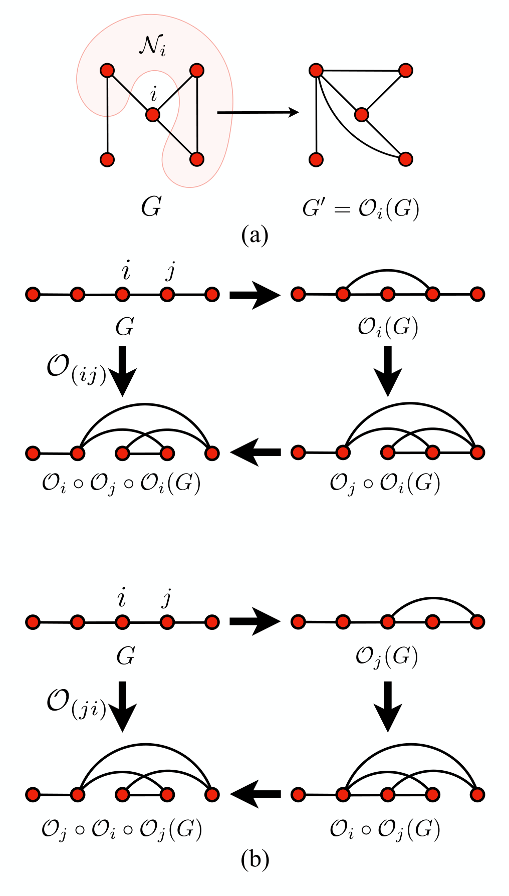
Local complementation Van den Nest et al. 2004b; Van den Nest et al. 2004c; Hein et al. 2006; Bouchet 1991; Bouchet 1993 of a connected graph $G$ w. r. t. a node $i\in G$ is a simple local graph operation, performed by deleting (creating) all the links $(j,k)$ between the nodes $j$ and $k$ $\in\mathcal{N}_{i}$ , if $(j,k)$ is present (absent) in the graph. Here, $\mathcal{N}_{i}$ is the neighborhood of the node $i$ , constituted of all the nodes in the graph that are connected to the node $i$ via a link. An example of the local complementation operation is demonstrated in Fig. 19(a) for a graph with $5$ nodes. Let $G^{\prime}=\mathcal{O}_{i}(G)$ represents the graph resulting from the local complementation on the node $i$ in $G$ . The corresponding graph states, $\ket{G^{\prime}}$ and $\ket{G}$ , are connected by an LC operation on the node $i$ and its neighboring nodes, as Van den Nest et al. 2004a $\ket{G^{\prime}}=U_{\text{LC}}^{i}\ket{G}$ , with

\displaystyle U_{\text{LC}}^{i}

\displaystyle=

\displaystyle\text{e}^{-\text{i}\frac{\pi}{4}\sigma^{1}_{i}}\otimes_{j\in\mathcal{N}_{i}}\text{e}^{\text{i}\frac{\pi}{4}\sigma^{3}_{j}}

(57)

Local complementation along an edge

Local complementation along an edge $(i,j)\in G$ is a sequence of three local complementations on $G$ w.r.t the nodes $i$ and $j$ , given by $\mathcal{O}_{(ij)}=\mathcal{O}_{i}\circ\mathcal{O}_{j}\circ\mathcal{O}_{i}$ , where $\mathcal{O}_{j}\circ\mathcal{O}_{i}(G)=\mathcal{O}_{j}\left(\mathcal{O}_{i}(G)\right)$ . Local complementation along an edge is symmetric with an interchange of $i$ with $j$ , i.e., $\mathcal{O}_{(ij)}\equiv\mathcal{O}_{(ji)}$ . This is demonstrated in Fig. 19(b) in the case of a linear graph with $5$ nodes. Evidently, local complementation along an edge represents a local unitary operation on the corresponding graph state, which is constituted by the unitaries of the form $U^{i}_{\text{LC}}$ , as given in Eq. (57).

Flip

The flip operation $\mathcal{F}_{i}^{a}$ on the node $i$ in $G$ reverses one of the binary attributes, shape, fill, and sign of the node, where the superscript $a$ in $\mathcal{F}_{i}^{a}$ represents the value of the flipped binary attribute, with $a=s,f,sg$ . The flip operations are consolidated in Fig. 20.

Reshape

Reshaping is an operation that is specific to the shape attribute of a node. We denote this operation by $\mathcal{R}_{i}^{s}$ , where the superscript $s$ is the shape attribute of the node prior to applying $\mathcal{R}^{s}_{i}$ , on which the action of $\mathcal{R}^{s}_{i}$ depends. If the shape of a node is a circle, then $\mathcal{R}_{i}^{c}$ results in only a flip of the shape that changes the shape attribute from circle to diamond, i.e., $\mathcal{R}_{i}^{c}\equiv\mathcal{F}_{i}^{c}$ . On the other hand, if the shape of a node is a diamond, then $\mathcal{R}_{i}^{d}$ is equivalent to (a) a flip of the shape that changes the shape attribute from diamond to circle, and (b) a flip of the sign from $+$ ( $-$ ) to $-$ ( $+$ ). These rules are also consolidated in Fig. 20.

A.1 Obtaining the reduced graph

We now discuss the graph transformation $G\rightarrow G^{\prime}_{\alpha}$ for a specific choice of the PMS $\alpha$ , which is a key ingredient of the protocol for computing $E^{\mathcal{P}}_{S}$ over an arbitrary $S$ in an arbitrary $G$ , as discussed in Sec. III.2.1. Starting from $\rho$ corresponding to an arbitrary graph $G$ , we achieve this in two steps, Step A and Step B. In Step A, we graphically represent the state $\rho_{\alpha}=\mathbf{U}^{\dagger}_{\alpha}\rho\mathbf{U}_{\alpha}$ (see Eq. (22)). Next, we perform Step B to obtain the graphical representation of the state $\rho^{\prime}_{\alpha}=\mathbf{V}_{\alpha}\ket{G^{\prime}_{\alpha}}\bra{G^{\prime}_{\alpha}}\mathbf{V}^{\dagger}_{\alpha}$ , from which the graph $G^{\prime}_{\alpha}$ can be straightforwardly extracted.

Step A. As stated in Sec. III.2.1, we are specifically interested in the single-qubit unitary operations $\{\sigma^{3}_{i},H_{i},R_{i}\}$ on the qubit $i$ . Based on the graph operations described above, these unitaries can be represented as follows Elliott et al. 2008; Elliott et al. 2009.

A.1

$H_{i}$ on any node: $\mathcal{F}_{i}^{f}$ ( $\mathcal{F}_{i}^{r}(G)$ or $\mathcal{F}_{i}^{w}(G)$ , depending on whether $f=r$ or $w$ for the node $i$ ).
A.2

$R_{i}$ on a node with $f=r$ : $\mathcal{R}_{i}^{s}$ ( $\mathcal{R}_{i}^{c}(G)$ or $\mathcal{R}_{i}^{d}(G)$ , depending on whether $s=c$ or $d$ for the node $i$ ).
A.3

$R_{i}$ on a node with $f=w$ , $s=c$ , $sg=+$ : $\mathcal{R}^{s}_{\mathcal{N}_{i}}\circ\mathcal{O}_{i}$ , where $\mathcal{R}^{s}_{\mathcal{N}_{i}}$ represents $\mathcal{R}^{s}_{j}$ operations on all nodes $j\in\mathcal{N}_{i}$ .
A.4

$R_{i}$ on a node with $f=w$ , $s=c$ , $sg=-$ : $\mathcal{F}^{sg}_{\mathcal{N}_{i}}\circ\mathcal{R}^{s}_{\mathcal{N}_{i}}\circ\mathcal{O}_{i}$ , where $\mathcal{R}^{s}_{\mathcal{N}_{i}}$ represents $\mathcal{R}^{s}_{j}$ operations on all nodes $j\in\mathcal{N}_{i}$ , and $\mathcal{F}^{sg}_{\mathcal{N}_{i}}$ stands for $\mathcal{F}^{sg}_{j}$ $\forall j\in\mathcal{N}_{i}$ .
A.5

$R_{i}$ on a node with $f=w$ , $s=d$ , $sg=+$ : $\mathcal{F}^{sg}_{\mathcal{N}_{i}}\circ\mathcal{R}^{s}_{\mathcal{N}_{i}}\circ\mathcal{O}_{i}\circ\mathcal{F}^{d}_{i}\circ\mathcal{F}^{w}_{i}$ where $\mathcal{F}^{sg}_{\mathcal{N}_{i}},\mathcal{R}^{s}_{\mathcal{N}_{i}}$ denotes flip and reshape operations respectively on entire neighbourhood of the node.
A.6

$R_{i}$ on a node with $f=w$ , $s=d$ , $sg=-$ : $\mathcal{R}^{s}_{\mathcal{N}_{i}}\circ\mathcal{O}_{i}\circ\mathcal{F}^{d}_{i}\circ\mathcal{F}^{w}_{i}$
A.7

$\sigma^{3}_{i}$ on a node with $f=r$ : $\mathcal{F}^{sg}_{i}$ ( $\mathcal{R}_{i}^{+}(G)$ or $\mathcal{R}_{i}^{-}(G)$ , depending on whether $sg=\pm$ for the node $i$ )
A.8

$\sigma^{3}_{i}$ on a node with $f=w$ , $s=c$ : $\mathcal{F}_{\mathcal{N}_{i}}^{sg}$ . Where $\mathcal{F}^{sg}_{\mathcal{N}_{i}}$ denotes flip of sign on all neighbourhood nodes.
A.9

$\sigma^{3}_{i}$ on a node with $f=w$ , $s=d$ : $\mathcal{F}^{sg}_{i}\circ\mathcal{F}_{\mathcal{N}_{i}}^{sg}$

For ease of representation, we denote the graph operations corresponding to the rules $A.1,\cdots,A.9$ as $\mathcal{A}_{1},\cdots,\mathcal{A}_{9}$ , where, for example, $\mathcal{A}_{3}\equiv\mathcal{R}_{\mathcal{N}_{i}}^{s}\circ\mathcal{O}_{i}$ . Note that a subset of the transformations $\{\mathcal{A}_{1},\cdots,\mathcal{A}_{9}\}$ according to a specific unitary operator $\mathbf{U}_{\alpha}$ corresponding to a specific PMS $\alpha$ provides a graphical representation of the state $\rho_{\alpha}$ (see Eq. (22) and the corresponding discussions).

Step B. To achieve this step, we additionally use two graph transformations, referred to as the equivalence transformations, that correspond to Eq. (23) in Sec. III.2.1. These graph transformations, denoted by $\mathcal{B}_{1}$ and $\mathcal{B}_{2}$ , are described below.

B.1

The graph operations constituting $\mathcal{B}_{1}$ on a node $i$ with $s=d$ are as follows, in the specified order: (1) flip the fill of the node $i$ , (2) perform local complementation on the node $i$ , (3) reshape the neighbors of the node $i$ in the transformed graph, (4) flip the sign of the node $i$ , and (5) if $sg=-$ for the node $i$ in the resulting graph, then flip the signs of the neighbors of the node $i$ in the transformed graph also.
B.2

The graph operations constituting $\mathcal{B}_{2}$ on a link $(i,j)\in G$ , such that both $i$ and $j$ have $s=c$ , are as follows, in the specified order: (1) flip the fills of the nodes $i$ and $j$ , (2) perform a local complementation along the edge $(i,j)$ , (3) flip the signs of the nodes that are connected to both of $i$ and $j$ in the transformed graph, and (4) if either of the nodes $i$ and $j$ in the transformed graph has $sg=-$ , flip the sign of that node as well as the signs of its neighbors in the transformed graph.

We now present the algorithm for obtaining $G^{\prime}_{\alpha}$ in the form of a pseudo code, using the above equivalence transformations.

input (1) The graphical representation of $\rho_{\alpha}$ , as obtained from Step A, with nodes of eight different attributes and the links, and (2) sets $S^{\prime}$ and $S$ of measured and unmeasured nodes.

1.
obtain the set $\mathcal{D}_{dw}$ of all nodes with $s=d$ , $f=w$ (i.e., type $7$ and type $8$ nodes (see Fig. 18)), and the set $\mathcal{L}_{cw}$ of all pairs $(i,j)$ of nodes with $s=c$ , $f=w$ , (i.e., (type $3$ , type $3$ ), (type $3$ , type $4$ ), (type $4$ , type $3$ ), and (type $4$ , type $4$ ) links) such that the link $(i,j)$ exists. The sizes of these sets are given by $|\mathcal{D}_{dw}|$ and $|\mathcal{L}_{cw}|$ , respectively.
1. (a)
  while $|\mathcal{L}_{cw}|>0$ or $|\mathcal{D}_{dw}|>0$ , do
  1. (I)
    
    operate $\mathcal{B}_{1}$ on all nodes $i\in\mathcal{D}_{dw}$
  2. (II)
    
    operate $\mathcal{B}_{2}$ on all $(i,j)\in\mathcal{L}_{cw}$
2. (b)
  
  determine $|\mathcal{L}_{cw}|$ , $|\mathcal{D}_{dw}|$ .
3. (c)
  
  if $|\mathcal{L}_{cw}|>0$ or $|\mathcal{D}_{dw}|>0$ , repeat (a)-(c).
4. else exit
2.
obtain the set $\mathcal{E}_{B}$ of all boundary links $(i,j)$ having node $i\in S^{\prime}$ , and node $j\in S$ , such that $i$ is either of type $3$ , type $4$ nodes (see Fig. 18). Let us denote the set of these nodes $i\in S^{\prime}$ as $\mathcal{N}_{S}$ .
1. (a)
  for all $(i,j)\in\mathcal{E}_{B}$ such that $i\in\mathcal{N}_{S}$ , do
  1. (I)
    
    if $j$ has $s=c$ , apply $\mathcal{B}_{2}$ on $(i,j)$
  2. else first apply $\mathcal{B}_{1}$ to node $j$ , and then to node $i$
3.

extract the unitary operation $\mathbf{V}$ from the node attributes
4.

replace all nodes by type 1 nodes (see Fig. 18) converting it to a normal graph, and extract the connectivity of $G^{\prime}_{\alpha}$ .

output (1) The reduced graph $G^{\prime}_{\alpha}$ , and (2) the unitary $\mathbf{V}$ in terms of the set of unitaries $\{V_{i},i\in G^{\prime}_{\alpha}\}$ .

Implementation of the algorithm presented in the pseudo code upto step 2 ensures the following for $\rho^{\prime}_{\alpha}$ .

(a)

The neighborhood $S_{1}^{\prime}$ of $S$ has at least one node, and the nodes in $S_{1}^{\prime}$ can be only of the types $1$ , $2$ , $5$ , or $6$ (see Fig. 18), so that $\sigma^{3}$ measurement on these nodes remain unchanged.
(b)

The nodes in $S_{2}^{\prime}$ , in addition to being of the types $1$ , $2$ , $5$ , or $6$ , can also be of the types $3$ or $4$ (see Fig. 18). This ensures that only $\sigma^{3}$ and $\sigma^{1}$ measurements are allowed in $S_{2}^{\prime}$ .
(c)

If a type $3$ node, or a type $4$ node occurs in $S_{2}^{\prime}$ , then its neighborhood will be constituted of types $1$ , $2$ , $5$ , and $6$ nodes only.

Because of these characteristics of $\rho^{\prime}_{\alpha}$ , it is always possible to fully disconnect types $3$ and $4$ nodes of $S_{2}^{\prime}$ by measuring $\sigma^{3}$ only on the nodes of types $1$ , $2$ , $5$ , and $6$ . Note that when $\sigma^{3}$ is measured on a node $i\in\{\text{type }1,\text{type }2,\text{type }5,\text{type }6\}$ , the outcomes $\pm 1$ are equiprobable, and the graph post-measurement can be obtained by

1.

deleting all the edges between the node $i$ and its neighbours $\mathcal{N}_{i}$ ,
2.

replacing the node $i$ with type $3$ (type $4$ ) node if the outcome is $+1$ ( $-1$ ), and
3.

performing $\mathcal{F}_{\mathcal{N}_{i}}^{sg}$ if the outcome is $-1$ .

If one now measures $\sigma^{3}$ on a node $i\in\{\text{type }3,\text{type }4\}$ belonging to $S_{2}^{\prime}$ , due to the absence of connection between the node and the rest of the graph, the measurement leaves the graph unaltered, and the measurement outcome is $+1$ ( $-1$ ) for the node of type $3$ (type $4$ ) with certainty.

A.2 Scaling with system-size

We now explore how the protocol discussed in Sec. III.2.1 and Appendix A scales with the number of measured nodes $|S^{\prime}|=N-n=m$ in a graph $G$ , which is given by the dependence of the total number of graph operations, $C$ , performed during the protocol on $m$ . Since the graph $G$ changes during each step of the protocol, it is in general difficult to obtain the exact dependence of $C$ on $m$ . However, to estimate an upper bound, $C^{\prime}$ , of $C$ , consider a fully connected graph of size $N$ , where $\sigma^{2}$ measurement⁹⁹ 9 This is the costliest Pauli measurement in terms of graph operations. See Appendix A. on $m$ nodes are performed so that a maximum number of graph operations in terms of flipping of the node attributes and creation or deletion of the links in local complementations have to be performed. The measurement transformation $\sigma^{2}\rightarrow\sigma^{3}$ in Step A on $m$ nodes corresponds to $2m$ graph operations. On the other hand, the number of graph operations during the reduction in Step B is upper bounded by $m$ iteration of $\mathcal{B}_{1}$ , each of which requires at most $N^{2}-N+4$ graph operations. Therefore, the dependence of $C$ on $m$ is overall upper bounded by

C^{\prime}=m(N^{2}-N+6).

(58)

In the limit $N\approx m$ ¹⁰¹⁰ 10 This is typically the case when the actual system is large enough compared to the subsystem on which entanglement is localized.

C^{\prime}=m^{3}-m^{2}+6m,

(59)

which is a polynomial dependence on $m$ .

In order to test this estimate, in Fig. 22, we present the numerical data for the variation of $C$ with $m$ , for cubic, square, and linear graphs states on $N=8^{3}=343$ , $N=18^{2}=324$ , and $N=325$ nodes, respectively. We randomly choose $n$ nodes from the graph, and perform $\sigma^{2}$ measurement on $m=N-n$ nodes, followed by a calculation of $C$ . We see that the numerical data is always upper bounded by $C^{\prime}$ , as per our estimation. Note here that the actual values of the total graph operations depend on the structure of the chosen graph, as expected.

Figure 22: Variation of the total number of graph operations with the number of measured nodes,

m

, in cubic, square and linear graphs on respectively

N=343,324

, and

325

nodes. To draw the variation of the analytically estimated upper bound,

C^{\prime}

, we use

N=324

Appendix B Proof of Proposition 1

Proof.

For reasons that will be clear shortly, we relabel the measurement outcomes corresponding to qubits in $S^{\prime}_{1}$ $(S^{\prime}_{2})$ by $l$ $(m)$ , such that $l_{j}=k_{j}$ ( $m_{j}=k_{j}$ ) if $j\in S^{\prime}_{1}$ ( $S^{\prime}_{2}$ ). We can therefore regroup the outcome-index $k$ as $k\equiv lm$ with $l\equiv l_{1}l_{2}\dots l_{L}$ , and $m\equiv m_{L+1}m_{L+2}\dots m_{N}$ , where we have assumed, without any loss in generality, that $L$ is the size of $S^{\prime}_{1}$ such that $S^{\prime}_{2}$ has $N-n-L$ qubits. In this notation, $M^{\alpha}_{k}\equiv M_{lm}^{\alpha}$ , and using Eq. (23) in Eq. (21), we obtain

	$\displaystyle\varrho_{k}$	$\displaystyle=$	$\displaystyle\mathbf{U}_{\alpha}M_{lm}^{\alpha}\rho_{\alpha}M_{lm}^{\alpha\dagger}\mathbf{U}^{\dagger}_{\alpha}$		(60)
		$\displaystyle=$	$\displaystyle\mathbf{U}_{\alpha}\mathbf{V}_{\alpha}M_{lm}^{\alpha}\ket{G^{\prime}_{\alpha}}\bra{G^{\prime}_{\alpha}}M_{lm}^{\alpha\dagger}\mathbf{V}^{\dagger}_{\alpha}\mathbf{U}^{\dagger}_{\alpha},$		(60)

with $M_{lm}^{\alpha}\leftarrow\mathbf{V}_{\alpha}^{\dagger}M_{lm}^{\alpha}\mathbf{V}_{\alpha}$ , such that after this transformation, $\alpha_{j}=3$ only $\forall j\in S^{\prime}_{1}$ . Note that $\mathbf{V}_{\alpha}$ can change only the measurement basis, not the measurement outcome. The graph transformation algorithm discussed in Appendix A ensures that the measurement on any of the qubits in $S_{2}^{\prime}$ can be either a $\sigma^{3}$ , or a $\sigma^{1}$ , i.e., $\alpha_{j}=1,3$ if $j\in S^{\prime}_{2}$ . Now, application of $M^{\alpha}_{lm}$ on the graph state $\ket{G^{\prime}_{\alpha}}$ results in the normalized state of the form

	$\displaystyle M_{lm}^{\alpha}$		$\displaystyle\ket{G^{\prime}_{\alpha}}\bra{G^{\prime}_{\alpha}}M_{lm}^{\alpha\dagger}=\mathbf{W}_{lm}\big[\left(\otimes_{j\in S^{\prime}_{1}}\ket{l_{j}}\bra{l_{j}}\right)\otimes$		(61)
			$\displaystyle\left(\otimes_{j\in S^{\prime}_{2}}\ket{m_{j}}\bra{m_{j}}\right)\otimes\left(\ket{G^{\alpha}_{S}}\bra{G^{\alpha}_{S}}\right)\big]\mathbf{W}_{lm}^{\dagger},$		(61)

where $G^{\alpha}_{S}$ is the subgraph on $S$ in $G^{\prime\prime}_{\alpha}$ , which is obtained by performing the graph transformations corresponding to the single-qubit Pauli measurements on the graph $G^{\prime}_{\alpha}$ for all qubits in $S^{\prime}$ . These transformations, for a measurement on a single qubit, are given by Hein et al. 2004; Hein et al. 2006

	$\displaystyle\sigma^{1}_{j}:\quad$	$\displaystyle G^{\prime}_{\alpha}$	$\displaystyle\rightarrow\mathcal{O}_{a}(\mathcal{O}_{j}(\mathcal{O}_{a}(G^{\prime}_{\alpha}))\backslash j),$		(62)
	$\displaystyle\sigma^{3}_{j}:\quad$	$\displaystyle G^{\prime}_{\alpha}$	$\displaystyle\rightarrow G^{\prime}_{\alpha}\backslash j,$		(63)

with $a$ being any node in the neighborhood $\mathcal{N}_{j}$ of the node $j\in G^{\prime}_{\alpha}$ , and $G^{\prime}_{\alpha}\backslash j$ is obtained from $G^{\prime}_{\alpha}$ by deleting all links connected to the node $j$ . The graph operation $\mathcal{O}_{j}(G)$ w.r.t. a node $j$ represents a local complementation Van den Nest et al. 2004b; Van den Nest et al. 2004c; Hein et al. 2006; Bouchet 1991; Bouchet 1993 operation (see also Appendix A for the definition). These single-qubit Pauli measurements on all $j\in S^{\prime}$ also results in Clifford unitary operators operating post-measurement on the qubits constituting the graph, leading to the unitary operations $\mathbf{W}_{lm}$ , given by Hein et al. 2004; Hein et al. 2006

\displaystyle\mathbf{W}_{lm}

\displaystyle=

\displaystyle\left(\otimes_{j\in S^{\prime}_{1}}W_{l_{j}}^{3}\right)\left(\otimes_{j\in S^{\prime}_{2}}W_{m_{j}}^{1,3}\right),

(64)

where for each $j$ ,

$\displaystyle W_{+1}^{1}$	$\displaystyle=$	$\displaystyle\text{e}^{\text{i}\frac{\pi}{4}\sigma^{2}_{a}}\otimes_{b\in\mathcal{N}_{j}\backslash(\mathcal{N}_{a}\cup a)}\sigma^{3}_{b},$	(65)
$\displaystyle W_{-1}^{1}$	$\displaystyle=$	$\displaystyle\text{e}^{-\text{i}\frac{\pi}{4}\sigma^{2}_{a}}\otimes_{b\in\mathcal{N}_{a}\backslash(\mathcal{N}_{j}\cup j)}\sigma^{3}_{b},$	(66)
$\displaystyle W^{3}_{+1}$	$\displaystyle=$	$\displaystyle I_{j},$	(67)
$\displaystyle W^{3}_{-1}$	$\displaystyle=$	$\displaystyle\otimes_{b\in\mathcal{N}_{j}}\sigma^{3}_{b},$	(68)

with $a$ being chosen as in Eq. (62).

It is worthwhile to point out here that Eqs. (62)-(63) indicate that $G^{\prime\prime}_{\alpha}$ , and consequently $G^{\alpha}_{S}$ is independent of the measurement outcomes $l$ and $m$ . Using (61) in Eq. (60), and tracing out the subsystem $S^{\prime}$ , we obtain

\displaystyle\varrho_{S}^{k}=\mathbf{V}_{S,\alpha}\mathbf{W}_{S,l}\ket{G^{\alpha}_{S}}\bra{G^{\alpha}_{S}}\mathbf{W}_{S,l}^{\dagger}\mathbf{V}_{S,\alpha}^{\dagger},

(69)

where the subscript $S$ is introduced in the unitary operators to signify the components of the unitaries that have support only on $S$ , and we have dropped the index $m$ from $\mathbf{W}_{S}$ as the components of $\mathbf{W}$ on $S$ are governed only by $l$ . Therefore,

\displaystyle E(\varrho_{S}^{k})=E\left(\ket{G^{\alpha}_{S}}\bra{G^{\alpha}_{S}}\right),

(70)

which is independent of the measurement outcomes $l$ and $m$ . This proves Proposition 1. ∎

Appendix C Entanglement in pure graph states

Here we discuss quantification and characterization of bipartite and multipartie entanglement in graph states.

C.1 Bipartite entanglement

Let us consider a system of qubits $V\equiv\{1,2,\cdots,N\}$ forming a connected graph $G$ . Let us now consider a bipartition of the system $V$ as $A\cup B=V$ , and $A\cap B=\emptyset$ , where $d_{A}=\dim(\mathcal{H}_{A})$ ( $d_{B}=\mathcal{H}_{B}$ ), $\mathcal{H}_{A}$ ( $\mathcal{H}_{B}$ ) being the Hilbert space associated to $A$ ( $B$ ). For each pure state $\ket{G}$ in $\mathcal{H}_{A}\otimes\mathcal{H}_{B}$ , orthonormal basis $\{b_{A}^{i}\}\in\mathcal{H}_{A}$ and $\{b_{B}^{j}\}\in\mathcal{H}_{B}$ exist such that in Schmidt decomposed form,

\displaystyle\ket{G}=\sum_{i=1}^{d}\sqrt{\lambda_{i}}\ket{b_{A}^{i}b_{B}^{i}},

(71)

with $d=\min\{d_{A},d_{B}\}$ , and non-negative Schmidt coefficients $\sqrt{\lambda_{i}}$ with $\lambda_{i}\geq 0$ and $\sum_{i=1}^{d}\lambda_{i}=1$ . The marginals of $\ket{G}$ , given by

	$\displaystyle\rho_{A}(B)$	$\displaystyle=$	$\displaystyle\text{Tr}_{B(A)}[\ket{G}\bra{G}]$		(72)
		$\displaystyle=$	$\displaystyle\sum_{i=1}^{d}\lambda_{i}\ket{b_{A(B)}^{i}}\bra{b_{A(B)}^{i}},$		(72)

has the spectrum $\{\lambda_{i};i=1,\cdots,d\}$ . The state $\ket{G}$ is maximally entangled (ME) Horodecki et al. 2009; Gühne and Tóth 2009 in the bipartition $A:B$ if $\lambda_{i}=1/d$ $\forall i$ , which corresponds to the marginal of the subsystem of dimension $d$ to be maximally mixed, i.e., $I/d$ , where $I$ is the identity matrix on the Hilbert space of dimension $d$ . Otherwise, $\ket{G}$ is non-maximally entangled (NME) in the partition $A:B$ . In situations where $\ket{G}$ is maximally entangled across any bipartition (see also Gisin and Bechmann-Pasquinucci 1998; Higuchi and Sudbery 2000), they are referred to as the absolutely maximally entangled (AME) states Facchi et al. 2008; Gour and Wallach 2010; Arnaud and Cerf 2013; Goyeneche et al. 2015; Enríquez et al. 2016. To compute the bipartite entanglement $E_{A:B}(G)$ between the partitions $A$ and $B$ of $G$ , one needs to compute the marginals $\rho_{A(B)}$ for $\ket{G}$ , which can be obtained in terms of the generators $\tilde{g}_{i}^{A(B)}$ as Hein et al. 2004; Hein et al. 2006

\displaystyle\rho_{A(B)}

\displaystyle=

\displaystyle\frac{1}{d_{A(B)}}\sum_{\left\{\tilde{g}_{i}^{A(B)}\right\}}\tilde{g}_{i}^{A(B)},

(73)

where

\displaystyle\left\{\tilde{g}_{i}^{A(B)}\right\}=\left\{g_{i}|\text{supp}\left(g_{i}\right)\in A(B)\right\},

(74)

i.e., $\left\{\tilde{g}_{i}^{A(B)}\right\}$ is the subset of $\{g_{i}\}$ with support on $i\in A(B)$ . For an arbitrary connected graph $G$ , the single-qubit marginals corresponding to all qubits are maximally mixed Verstraete et al. 2003; Hein et al. 2006, implying $\ket{G}$ is ME in all bipartitions of a qubit and the rest. Also, note that for $N=2,3$ , $d=2$ (see Eq. (71)), and $\ket{G}$ is AME. On the other hand, in case of $G$ with arbitrary $N>3$ , and assuming $A$ to be the smaller subsystem constituted of $2$ qubits $\{i,j\}\in G$ (i.e., $d=4$ ), $\rho_{A}=\rho_{ij}$ is either maximally mixed, or a rank- $2$ mixed state Hein et al. 2006. In the case of the former, $\ket{G}$ is ME in the bipartition $A:B$ , whereas in the case of the latter, it is not.

Note that it is sufficient to investigate connected graphs. In the case of graphs that are not connected, the bipartite entanglement present in the graph will be decided by the bipartite entanglement present in the graph states corresponding to the connected segments of the full graph.

C.2 Multipartite entanglement

We now discuss the multipartite entanglement in graph states. A multi-qubit quantum state is genuinely multiparty entangled if it is not separable in any possible bipartition. Connected pure graph states are known to be genuinely multiparty entangled Hein et al. 2004, where the degree of entanglement can be quantified using the Schmidt measure Hein et al. 2004; Hein et al. 2006, and the generalized geometric measure Sen De; Sadhukhan et al. 2017.

C.2.1 Schmidt measure

A pure state of $N$ qubits can be written as

\ket{\psi}=\sum_{i=1}^{R}c_{i}\ket{\psi^{(1)}_{i}}\otimes...\otimes\ket{\psi^{(N)}_{i}},

(75)

where $c_{i}$ s are complex numbers subject to normalization $\sum_{i}|c_{i}|^{2}=1$ , $\ket{\psi^{(l)}_{i}}$ belongs to the Hilbert space of the qubit $l$ , $l=1,2,\dots,N$ , and $R$ is an integer $<2^{N}$ . The Schmidt measure of $\ket{\psi}$ is given by Hein et al. 2004; Eisert and Briegel 2001

E(\ket{\psi}\bra{\psi})=\log_{2}(r),

(76)

where $r$ is the minimum possible value of $R$ over all possible linear decompositions of $\ket{\psi}$ into product states. In general, Schmidt measure is a difficult one to compute for an arbitrary pure multi-qubit state. However, there exist computable lower and upper bounds of the measure for certain multi-qubit states, including the graph states. A lower bound to the Schmidt measure in the case of graph states can be obtained as follows Hein et al. 2004. For a given graph $G$ and a bipartition $A:B$ such that $G=A\cup B$ , the adjacency matrix $\Gamma_{G}$ can be written, without any loss in generality, as

\displaystyle\Gamma_{G}=\begin{pmatrix}\Gamma_{A}&\Gamma_{AB}^{T}\\ \Gamma_{AB}&\Gamma_{B}\end{pmatrix}

(77)

by rearranging the nodes, where $T$ denotes the transposition operation. The Schmidt measure of the graph state w.r.t. the partition $A:B$ is given by the rank of the matrix $\Gamma_{AB}$ , i.e,

E(\ket{G}\bra{G})=\text{rank}[\Gamma_{AB}].

(78)

The lower bound to the Schmidt measure w.r.t the partitioning of the system into smallest possible subsystems¹¹¹¹ 11 In the present case, each partition would hold one qubit. is given by maximizing $E(\ket{G}\bra{G})$ over all possible bipartitions Hein et al. 2004, as

E_{L}(\ket{G}\bra{G})=\max_{\forall\{A:B\}}E(\ket{G}\bra{G}).

(79)

On the other hand, an upper bound to Schmidt measure in the case of graph states is given by the Pauli persistency, defined as the minimum number of local Pauli measurements required to completely disentangle the state Hein et al. 2004. We exploit the measurement protocol for the evaluation of this upper bound as follows. For a graph state $\ket{G}$ on $N$ qubits, and for a chosen Pauli measurement setup $\mathcal{P}$ on these $N$ qubits, let us denote the the reduced graph, obtained according to Eq.(23), by $G^{\prime}$ . The minimal vertex cover of this reduced graph $G^{\prime}$ is defined as the minimum cardinality of the subset of nodes in $G^{\prime}$ such that upon deletion of edges on them leaves behind a completely disconnected graph on $N$ vertices and we denote it by $M(G^{\prime})$ . An upper bound to the Schmidt measure of $\ket{G}$ is given by minimizing $M(G^{\prime})$ over all possible Pauli measurements i.e,

E_{U}(\ket{G}\bra{G})=\min_{\mathcal{P}}M(G^{\prime}).

(80)

C.2.2 Generalized geometric measure

Let us consider a $K$ -separable $N$ -qubit quantum state $\ket{\phi_{K}}$ , which can be divided into $K$ product state partitions, where $2\leq K\leq N$ . The GME in an $N$ -qubit state $\ket{\psi}$ is quantified by the $K$ -geometric measure (K-GM) of entanglement, defined as the minimum distance of the state $\ket{\psi}$ from the set $\mathcal{S}_{K}$ of all possible $K$ -separable states, i.e.,

\displaystyle E(\ket{\psi})=1-\underset{\mathcal{S}_{K}}{\max}|\langle{\phi_{K}}|\psi\rangle|^{2}.

(81)

The original definition of the geometric measure is recovered for $K=N$ , while at the other extremum $K=2$ , the measure is called the generalized geometric measure (GGM). The optimization in the definition of the GGM can be achieved via a maximization of the Schmidt coefficients across all possible bipartitions of $\ket{\psi}$ Biswas et al. 2014, leading to

\displaystyle E=1-\underset{\mathcal{S}_{A:B}}{\max}\{\lambda^{2}_{A:B}\},

(82)

where $\lambda_{A:B}$ is the Schmidt coefficient of $\ket{\psi}$ maximized over the set $\mathcal{S}_{A:B}$ of all arbitrary $A:B$ bipartitions of the $N$ -qubit system. The GGM of a pure state of arbitrary number of qubits, $N$ , can be computed using Eq. (82).

Appendix D Proof of Proposition 2

Proof.

Using

\displaystyle J_{s^{\prime\prime}}

\displaystyle=

\displaystyle J_{S,s^{\prime\prime}}\otimes J_{S^{\prime},s^{\prime\prime}}

(83)

and

\displaystyle q_{s}=q_{S,s}\times q_{S^{\prime},s}

(84)

with $q_{S(S^{\prime}),s}=\prod_{j\in S(S^{\prime})}q_{s_{j}}$ , and $\sum_{(S^{\prime},s)}q_{S^{\prime},s}=\sum_{(S,s)}q_{S,s}=1$ , one can trace out $S^{\prime}$ from $\varrho_{k}$ to obtain

\displaystyle\varrho^{k}_{S}=\mathbf{V}_{S,\alpha}\tilde{\varrho}^{k}_{S}\mathbf{V}_{S,\alpha}^{\dagger}

(85)

with

\displaystyle\tilde{\varrho}_{S}^{k}=\sum_{(S,s)}q_{S,s}J_{S,s^{\prime\prime}}\tilde{\rho}_{S}J_{S,s^{\prime\prime}}^{\dagger},

(86)

where $\tilde{\rho}_{S}$ is a GD state in the graph-state basis corresponding to the graph $G_{S}^{\alpha}$ on the subsystem $S$ , obtained from $G^{\prime}_{\alpha}$ (see Eq. (69)). We write $\tilde{\rho}_{S}$ as,

\displaystyle\tilde{\rho}_{S}=\sum_{\psi}\lambda_{\psi}(\alpha,s)\ket{\psi}\bra{\psi}

(87)

$\{\ket{\psi}\}$ being the graph basis in the Hilbert space of $S$ where $\psi\in[0,2^{n}-1]$ , and $\psi$ can be identified as $\psi\equiv\psi_{1}\psi_{2}\dots\psi_{n}$ , where $\psi_{i}\in\{0,1\}\forall i\in S$ . In this notation $\ket{0}\bra{0}\equiv\ket{G_{S}^{\alpha}}\bra{G_{S}^{\alpha}}$ , and (see Sec. III.1)

\displaystyle\ket{\psi}

\displaystyle=

\displaystyle\otimes_{i\in S}(\sigma_{i}^{3})^{\psi_{i}}\ket{G_{S}^{\alpha}}

(88)

Note that the mixing probabilities $\lambda_{\psi}(\alpha,s)$ are in general functions of the PMS, $\alpha$ , and the type of the noise, $s$ . These probabilities and subsequently the state $\tilde{\rho}_{S}$ can be calculated from the knowledge of the connectivity between the sets of qubits $S$ and $S_{1}^{\prime\prime}$ , where $S_{1}^{\prime\prime}\subseteq S_{1}^{\prime}$ such that $s_{j}=1,2$ $\forall j\in S_{1}^{\prime\prime}$ , i.e., the noise on $S_{1}^{\prime\prime}$ does not commute with the measurement, which is $\sigma^{3}$ for all qubits in $S_{1}^{\prime}$ . A technical account of the prescription for calculating $\tilde{\rho}_{S}$ is given in the Appendix F for the interested readers.

Note further that an application of Eq. (86) on $\tilde{\rho}_{S}$ leads to another GD state on $S$ . To determine this, we (a) first obtain the GD state resulting from the application of Eq. (86) on $\ket{\psi}\bra{\psi}\equiv\ket{0}\bra{0}=\ket{G^{\alpha}_{S}}\bra{G^{\alpha}_{S}}$ (using Eq. (IV.1)) as

	$\displaystyle\sum_{(S,s)}q_{S,s}J_{S,s^{\prime\prime}}\ket{0}\bra{0}J_{S,s^{\prime\prime}}^{\dagger}=\sum_{\psi^{\prime}}\lambda_{\psi^{\prime}}(\alpha,s)\ket{\psi^{\prime}}\bra{\psi^{\prime}},$
			(89)

and (b) then use Eqs. (87) and (89) in Eq. (86), with the aid of Eq. (88), to obtain

	$\displaystyle\tilde{\varrho}^{k}_{S}$	$\displaystyle=$	$\displaystyle\sum_{(S,s)}q_{S,s}J_{S,s^{\prime\prime}}\left[\sum_{\psi}\lambda_{\psi}\ket{\psi}\bra{\psi}\right]J_{S,s^{\prime\prime}}^{\dagger}$		(90)
		$\displaystyle=$	$\displaystyle\sum_{\psi,\psi^{\prime}}\lambda_{\psi}\lambda_{\psi^{\prime}}\ket{\psi\oplus\psi^{\prime}}\bra{\psi\oplus\psi^{\prime}},$		(91)

where $\psi\oplus\psi^{\prime}$ represents modular two addition of the binary strings $\psi$ and $\psi^{\prime}$ . Also to arrive at Eq. (91), we use $\sigma^{3}\sigma^{j}\sigma^{3}=\sigma^{j},j\in\{1,2,3\}$ upto irrelevant multiplicative factors.

From Eq. (85), it is clear that

\displaystyle E(\varrho^{k}_{S})=E(\tilde{\varrho}^{k}_{S}).

(92)

Moreover, note that for two distinct outcomes $k_{1}$ and $k_{2}$ having their respective components in $S_{1}^{\prime\prime}$ as $l^{\prime}_{1}$ and $l^{\prime}_{2}$ ¹²¹² 12 Note that $l_{1}^{\prime}$ and $l_{2}^{\prime}$ can be seen as the parts of corresponding $l^{\prime}$ s that belong to $S^{\prime\prime}_{1}$ , $l_{2}^{\prime}=l^{\prime}_{1}\oplus L^{\prime}$ in binary representation, where $L^{\prime}$ is another binary string of the same length as $l^{\prime}_{1},l_{2}^{\prime}$ . Therefore, a sum over $l_{1}^{\prime}$ (see Eq. (47)¹³¹³ 13 Note that the sum over $s$ in Eq. (47) can be seen as an effective sum over all possible $l_{1}^{\prime}$ is equivalent to a sum over $l^{\prime}_{2}$ for a fixed $L^{\prime}$ . This results in local unitary connected states for the two outcomes $k_{1}$ and $k_{2}$ as

\displaystyle\tilde{\varrho}^{k_{1}}_{S}=\mathbf{W}^{L^{\prime}}_{S}\tilde{\varrho}^{k_{2}}_{S}\mathbf{W}^{L^{\prime}}_{S},

(93)

where $\mathbf{W}^{L^{\prime}}_{S}$ is a local unitary operator acting on $S$ , having the form,

\mathbf{W}^{L^{\prime}}_{S}=\prod_{j\in S_{1}^{\prime\prime}}\otimes_{i\in\mathcal{N}_{j}\cap S}(\sigma^{3}_{i})^{L_{j}^{\prime}},

(94)

where $L^{\prime}_{j}$ is the outcome on the $j$ th qubit, $j\in S_{1}^{\prime\prime}$ . Therefore, $E(\tilde{\varrho}^{k_{1}}_{S})=E(\tilde{\varrho}^{k_{2}}_{S})$ for any two distinct outcomes $k_{1},k_{2}$ , which, along with Eq. (92), leads to

\displaystyle E_{S}(\varrho^{k_{1}}_{S})=E_{S}(\varrho^{k_{2}}_{S}).

(95)

Hence the proof. ∎

Appendix E Calculating localizable entanglement for the graph in Fig. 2 under noise

To demonstrate the calculation of localizable entanglement in the presence of noise, we consider the graph in Fig. 2(a), where each qubit is subjected to BPF noise.

E.1 When no outcomes are forbidden

Let us consider $\sigma^{3}$ measurements performed on qubits $1$ and $2$ constituting $S^{\prime}$ . Since $U_{j}=V_{j}=I$ corresponding to qubits $j=1,2$ in the case depicted in Fig. 2(a), the reduced graph is equivalent to the original graph, and $s^{\prime\prime}=s^{\prime}=s$ in Eqs. (41)-(47). The change $l_{1}\rightarrow l_{1}^{\prime}$ and $m_{2}\rightarrow m_{2}^{\prime}$ in Eq. (47) due to the values of $s$ , according to Eq. (46), are tabulated in Table 2A. Note that in this specific example, all four measurement outcomes $k\equiv l_{1}m_{2}$ are equally probable, and remain so even after the change $l_{1}\rightarrow l_{1}^{\prime}$ and $m_{2}\rightarrow m_{2}^{\prime}$ . Since both qubits in $S^{\prime\prime}_{1}=\{1,2\}$ are connected to the two qubits in $S$ , the normalized state $\tilde{\rho}_{S}$ (see Eq. (87)) corresponding to outcome $k=(+1)(+1)\equiv 00$ , occurring with a probability $1/4$ , can be written in a row vector notation as

\displaystyle\sum_{\psi}\lambda_{\psi}\ket{\psi}\bra{\psi}\equiv\bigg[1-q+\frac{q^{2}}{2},0,0,q-\frac{q^{2}}{2}\bigg]

(96)

where $\lambda_{\psi}$ is the value in the position $\psi$ of the row. Similarly, equivalent to Eq. (89), one may write

\displaystyle\sum_{\psi^{\prime}}\lambda_{\psi^{\prime}}\ket{\psi^{\prime}}\bra{\psi^{\prime}}\equiv\bigg[1-q+\frac{q^{2}}{2},0,0,q-\frac{q^{2}}{2}\bigg].

(97)

Combining the above equations in the case where $S_{2}^{\prime}=\emptyset$ and $k=l=(+1)(+1)\equiv 00$ , one obtains, equivalent to Eq. (91),

	$\displaystyle\tilde{\varrho}^{(+1)(+1)}_{S}$	$\displaystyle=$	$\displaystyle\bigg[\left(1-q+\frac{q^{2}}{2}\right)^{2}+\left(q-\frac{q^{2}}{2}\right)^{2},0,0,$		(98)
			$\displaystyle 2\left(1-q+\frac{q^{2}}{2}\right)\left(q-\frac{q^{2}}{2}\right)\bigg].$		(98)

The states $\tilde{\varrho}^{k}_{S}$ for $k=(+1)(-1),(-1)(+1),(-1)(-1)$ are also equally probable with probability $1/4$ , and can be obtained from $\tilde{\varrho}^{(+1)(+1)}_{S}$ via local unitary transformations, where the local unitary operators can also be seen from table 2A. For example outcomes $k=(+1)(+1)\equiv 00$ and $k=(-1)(+1)\equiv 10$ are connected by $L=10$ , and the corresponding states by the local unitary operator $\mathbf{W}^{L}_{S}=\sigma_{1}^{3}\otimes\sigma^{3}_{2}$ .

\alpha\in\Gamma

(all outcomes are allowed)

	$s_{1}=0,s_{2}=0$	$s_{1}=0,s_{2}=2$	$s_{1}=2,s_{2}=0$	$s_{1}=2,s_{2}=2$
$k\equiv l_{1}m_{2}$	$k^{\prime}\equiv l_{1}^{\prime}m_{2}^{\prime}$
$(+1)(+1)$	$(+1)(+1)$	$(+1)(-1)$	$(-1)(+1)$	$(-1)(-1)$
$(+1)(-1)$	$(+1)(-1)$	$(+1)(+1)$	$(-1)(-1)$	$(-1)(+1)$
$(-1)(+1)$	$(-1)(+1)$	$(-1)(-1)$	$(+1)(+1)$	$(+1)(-1)$
$(-1)(-1)$	$(-1)(-1)$	$(-1)(+1)$	$(+1)(-1)$	$(+1)(+1)$

\alpha\in\overline{\Gamma}

(some outcomes are allowed)

	$s_{1}=0,s_{2}=0$	$s_{1}=0,s_{2}=2$	$s_{1}=2,s_{2}=0$	$s_{1}=2,s_{2}=2$
$k\equiv l_{1}m_{2}$	$k^{\prime}\equiv l_{1}^{\prime}m_{2}^{\prime}$
$(+1)(+1)$ (a)	$(+1)(+1)$ (a)	$(+1)(-1)$ (f)	$(-1)(+1)$ (f)	$(-1)(-1)$ (a)
$(+1)(-1)$ (f)	$(+1)(-1)$ (f)	$(+1)(+1)$ (a)	$(-1)(-1)$ (a)	$(-1)(+1)$ (f)
$(-1)(+1)$ (f)	$(-1)(+1)$ (f)	$(-1)(-1)$ (a)	$(+1)(+1)$ (a)	$(+1)(-1)$ (f)
$(-1)(-1)$ (a)	$(-1)(-1)$ (a)	$(-1)(+1)$ (f)	$(+1)(-1)$ (f)	$(+1)(+1)$ (a)

Table 2: Change of outcomes due to Pauli noise on a qubit in the case of the example shown in Fig. 2, where BPF noise is applied to all qubits, and A.

\sigma^{3}

and B.

\sigma^{1}

measurements are performed on qubits

1

and

2

. In the case of B, allowed and forbidden outcomes are labelled by (a) and (f).

E.2 When forbidden set of outcomes is present

For $\alpha\in\overline{\Gamma}$ , there exists a set of outcomes that are forbidden (see Sec. III.2.2). In such cases, results discussed in the previous section hold except for the calculation of $\tilde{\rho}_{S}$ , and the explicit calculation depends on the fact that the change $lm\rightarrow l^{\prime}m^{\prime}$ may result in a transition between allowed and forbidden sets of outcomes. We demonstrate this using the graph shown in Fig. 2(a), where each qubit is subjected to BPF noise, and $\sigma^{1}$ measurements are performed on qubits $1$ and $2$ constituting $S^{\prime}$ . Since $U_{j}=H$ corresponding to qubits $j=1,2$ , and $V_{1}=H,V_{2}=I$ in this case, one has to work with the reduced graph shown in Fig. 2(b). Also, $s^{\prime\prime}=s^{\prime}=s$ in Eqs. (41)-(47), since BPF does not change under Hadamard operation. The transformations $l_{1}\rightarrow l_{1}^{\prime}$ and $m_{2}\rightarrow m_{2}^{\prime}$ in Eq. (47) due to the values of $s$ , according to Eq. (46), are tabulated in Table 2B. Since $S_{2}^{\prime}=\{1\}$ and $S^{\prime}_{1}=S^{\prime\prime}_{1}=\{2\}$ are connected to the two qubits in $S$ , $\tilde{\rho}_{S}$ corresponding to the outcome $k=lm=(+1)(+1)\equiv 00$ occurring with probability $(1-q+q^{2}/2)/2$ , can be written as (equivalent to Eq. (87))

\displaystyle\sum_{\psi}\lambda_{\psi}\ket{\psi}\bra{\psi}

\displaystyle\equiv

\displaystyle\bigg[\frac{1-q+\frac{q^{2}}{4}}{1-q+\frac{q^{2}}{2}},0,0,\frac{\frac{q^{2}}{4}}{1-q+\frac{q^{2}}{2}}\bigg],

It is worthwhile to point out that in contrast to the case discussed in Sec. E.1, the probabilities are no longer independent of $q$ – an artefact due to the transition between the outcomes belonging to the allowed and forbidden sets. Proceeding as before, one can write the normalized $\tilde{\varrho}^{(+1)(+1)}_{S}$ as

	$\displaystyle\tilde{\varrho}^{(+1)(+1)}_{S}$	$\displaystyle=$	$\displaystyle\bigg[1-q+\frac{q^{2}}{4}+\frac{(q-\frac{q^{2}}{2})\frac{q^{2}}{4}}{1-q+\frac{q^{2}}{2}},0,0,$		(100)
			$\displaystyle\frac{q^{2}}{4}+\frac{(q-\frac{q^{2}}{2})(1-q+\frac{q^{2}}{4})}{1-q+\frac{q^{2}}{2}}\bigg].$		(100)

In a similar fashion, one may also obtain $\tilde{\varrho}^{(+1)(-1)}_{S}$ as

\tilde{\varrho}^{(+1)(-1)}_{S}=\bigg[\frac{1}{2},0,0,\frac{1}{2}\bigg],

(101)

which clearly indicates that $\tilde{\varrho}^{(+1)(-1)}_{S}$ and $\tilde{\varrho}^{(+1)(+1)}_{S}$ are not connected by local unitary operators. Thus, in general, a local unitary connection among states corresponding to all the allowed outcomes does not exists, thereby taking away the advantage in the computation, as opposed to the case described in Sec. E.1, specifically in situations where the system-size is large. Note also that the outcomes which are initially forbidden at $q=0$ need not necessarily remain forbidden for $q>0$ . In the above example, $k=(-1)(+1)$ is forbidden at $q=0$ , but acquires a non zero probability $q(1-q/2)/2$ for $q>0$ .

Appendix F Determination of $\tilde{\rho}_{S}$

Here we discuss the calculation of $\tilde{\rho}_{S}$ (see Sec.D and Sec. E.1). Let us define $S_{1}^{\prime\prime}\subseteq S_{1}^{\prime}$ such that $S_{1}^{\prime\prime}$ consists of all nodes in $S_{1}^{\prime}$ that have $s^{\prime\prime}\in\{1,2\}$ . Let us further divide the nodes in $S^{\prime\prime}_{1}$ into $n$ classes, $n$ being the size of $S$ , such that the each of the nodes in the $m$ th class, $\mathcal{C}_{m}$ ( $m=1,2,\cdots,n$ ), is connected to $m$ nodes in $S$ . Since $m$ nodes from $S$ can be chosen in $\genfrac{(}{)}{0.0pt}{1}{n}{m}$ possible ways, the $m$ th class can be further divides into $\genfrac{(}{)}{0.0pt}{1}{n}{m}$ subclasses, which we denote by $\mathcal{C}^{r}_{m}$ , where each $\mathcal{C}_{m}^{r}$ has a size $|\mathcal{C}_{m}^{r}|$ , $1\leq r\leq\genfrac{(}{)}{0.0pt}{1}{n}{m}$ . See Fig. 23 for an example of a possible class structure in the case of $n=3$ .

Figure 23: Schematic representation of the class-structure of the subsystem

S^{\prime\prime}

of a graph, where entanglement is to be localized over a subsystem

S

of size

3

. To keep the figure uncluttered, only the subsystems

S^{\prime\prime}_{1}

S

, the links between

S^{\prime\prime}_{1}

and

S

, and the links between the nodes in

S

are drawn.

We once again use the binary representation to work using the graph state basis $\{\ket{\psi}\}$ (see Sec. D), where $\ket{G_{S}}=\ket{0}$ . The local unitary corrections (either $I$ or $\sigma^{3}$ ) applied to $\ket{G_{S}}$ can be represented in binary representation as

\displaystyle\ket{\psi}

\displaystyle=

\displaystyle\mathbf{W}^{\psi}\ket{0},\text{ with }\mathbf{W}^{\psi}=\otimes_{j=1}^{n}(\sigma^{3}_{j})^{\psi_{j}}.

(102)

In this representation, one can determine the effective correction of each of the subclasses $\mathcal{C}^{r}_{m}$ in the $m$ th class on $S$ by a parity bit, denoted by $\gamma(r,m)$ , such that for $\gamma(r,m)=0$ ( $\gamma(r,m)=1$ ), there will be no correction (a $\sigma^{3}$ correction) applied to each node in $S$ that are connected to the nodes in $\mathcal{C}^{r}_{m}$ (See Eqs.(67),(68)). The overall correction, denoted by $\mathbf{W}^{\psi}$ , applied on $S$ will be the product of all corrections due to all subclasses from all of the classes:

\mathbf{W}^{\psi}=\prod_{m=1}^{n}\prod_{r=1}^{\genfrac{(}{)}{0.0pt}{1}{n}{m}}(\sigma^{3}_{\mathcal{N}_{(r,m)}})^{\gamma(r,m)},

(103)

where $\mathcal{N}_{(r,m)}$ denotes the set of all nodes in $S$ connected to the subclass $C_{m}^{r}$ .

Note that there may exist different combinations of $\gamma(r,m)$ giving rise to the same correction $\mathbf{W}^{\psi}$ . For example, in the case of $n=3$ (Fig.(23), both $\gamma(r,m)=0\forall m,r$ and $\gamma(r,m)=1\forall m,r$ give rise to the trivial correction $I\otimes I\otimes I$ in S. Defining the total number of possible subclasses with $m\geq 2$ as

D=\sum_{m=2}^{n}{\genfrac{(}{)}{0.0pt}{1}{n}{m}},

(104)

there will be a total of $n+D$ subclasses for $S$ since $\genfrac{(}{)}{0.0pt}{1}{n}{1}=n$ . The purpose of this division into $D$ and $n$ will be evident soon. We now denote a binary string of $n+D$ bits as

	$\displaystyle\gamma=\gamma(1,1)\gamma(2,1)\dots\gamma(n,1)\gamma(1,2)\gamma(2,2)\dots\gamma(n,2)$
	$\displaystyle\dots\gamma(1,n)\gamma(2,n)\dots\gamma(1,n).$

The first $n$ of the parity bits in $\gamma$ are reserved for $m=1$ class, and the rest $D$ bits are assigned to the remaining $D$ subclasses of the classes $m=2,\cdots,n$ . In this notation mixing probabilities, $\lambda_{\psi}$ , are given by,

\displaystyle\lambda_{\psi}=\sum_{\gamma=0}^{2^{D}-1}\prod_{m=1}^{n}\prod_{r=1}^{\genfrac{(}{)}{0.0pt}{1}{n}{m}}P_{\gamma(r,m)}(r,m)

(106)

with

	$\displaystyle P_{\gamma(r,m)}(r,m)=\frac{1}{2}[1+(-1)^{\gamma(r,m)}(1-2q_{n})^{\|\mathcal{C}^{r}_{m}\|}],$
			(107)

and

\gamma(i,1)=\psi_{i}\oplus\bigoplus_{\begin{subarray}{c}\{(r,m)\},m>1\\ i\in\mathcal{N}_{(r,m)}\end{subarray}}\gamma_{(r,m)}

(108)

where $i$ denotes a qubit in $S$ , $i\in\mathcal{N}_{(r,m)}$ condition picks up only those subclasses in which a connection exists between $i$ and $\mathcal{C}_{m}^{r}$ , $\oplus$ denotes modular $2$ addition, and $q_{n}$ is the total probability of occurrence of change of outcome on a single qubit, $l_{j}\rightarrow l_{j}^{\prime}$ (see Eq. 46), for various noises considered in this paper. For an example $q_{n}=q/2$ for Markovian BF and $q_{n}=0$ for Markovian PD noises. An explicit calculation with $n=2$ can be found in Amaro and Müller 2020.

We point out here that the above calculation assumes identical noise strengths and non-Markovianity parameters on each qubit, irrespective of the type of noise present on the qubit in a specific subclass. However, one can also generalize to a scenario where $(q_{i},\epsilon_{i})$ on different qubits in a subclass are different, which originates from different $(q_{i},\epsilon_{i})$ on different qubits in the original graph. This leads to a form of $P_{\gamma(r,m)}(r,m)$ given by

	$\displaystyle P_{1}(r,m)$	$\displaystyle=$	$\displaystyle\sum_{\begin{subarray}{c}\beta=1,\\ \oplus\beta_{i}=1\end{subarray}}^{2^{\|\mathcal{C}_{m}^{r}\|}}\prod_{i\in\mathcal{C}_{m}^{r}}p_{i}^{\beta_{i}}(1-p_{i})^{1\oplus\beta_{i}},$
	$\displaystyle P_{0}(r,m)$	$\displaystyle=$	$\displaystyle 1-P_{1}(r,m),$		(109)

where $\beta=\beta_{1}\beta_{2}...\beta_{|\mathcal{C}_{m}^{r}|}$ is a multi-index with $\beta_{i}\in\{0,1\}$ , and $p_{i}$ is the probability of occurrence of noise on qubit $i$ , given by

\displaystyle p_{i}=\frac{q_{i}}{2}\left[1+\epsilon_{i}\left(1-\frac{q_{i}}{2}\right)\right]

(110)

for the BF and the BPF noise, and

\displaystyle p_{i}=\frac{q_{i}}{4}\left[1+3\epsilon_{i}\left(1-\frac{3q_{i}}{4}\right)\right]

(111)

for the DP noise. An example of this scenario can be found in Sec. IV.3.

Appendix G Entanglement in graph states under noise

In the presence of noise, and for states with more than two qubits, the problem of quantifying entanglement is significantly more complicated. For a given bipartition of a graph state under Pauli noise, the bipartite entanglement can be quantified by negativity Vidal and Werner 2002. On the other hand, for certain class of mixed states obtained when graph states are subjected to noise, such as the graph-diagonal states, useful criteria for detecting multipartite entanglement directly from the density matrix of the state exists Gühne and Seevinck 2010; Gühne et al. 2011. One can also compute a genuine multiparty concurrence Hashemi Rafsanjani et al. 2012 for graph states under noise with an $X$ -state as the density matrix. We briefly discuss these in this section.

G.1 Negativity as a bipartite measure for a graph-diagonal state

For a graph-diagonal state $\rho$ representing a graph with two partitions $A$ and $B$ , the negativity between $A$ and $B$ is defined as Vidal and Werner 2002

\displaystyle\mathcal{N}_{AB}=\frac{||\rho^{T_{A}}||-1}{2},

(112)

where $T_{A}$ denotes the transposition of $\rho$ w.r.t. the subsystem $A$ , and $||\mathcal{A}||=\text{Tr}\left[\sqrt{\mathcal{A}^{\dagger}\mathcal{A}}\right]$ for the matrix $\mathcal{A}$ .

G.2 Genuine multiparty entanglement in graph diagonal states

Determination of the multipartite entanglement measures is difficult in the case of mixed states. However, in the case of specific types of mixed states, such as the graph diagonal states of certain types or number of parties, criteria for the state to be genuine multiparty entangled, or biseparable, or fully separable can be determined using the density matrix of the state Gühne and Seevinck 2010. We first consider the example of a mixed state of $N$ qubits which is diagonal in the graph state basis (see Eqs. (4)-(6)) corresponding to an $N$ -qubit star graph, where

\displaystyle\ket{G}

\displaystyle=

\displaystyle\frac{1}{\sqrt{2}}\left[\ket{0_{0}}\otimes_{i=1}^{N-1}\ket{+_{i}}+\ket{1_{0}}\otimes_{i=1}^{N-1}\ket{-_{i}}\right],

with the node “ $0$ ” being the hub to which all other nodes $i=1,2,\cdots,N-1$ , are attached. We refer to this state as the star-graph-diagonal (SGD) state. Since an $N$ -qubit star graph can be converted to the $N$ -qubit GHZ state via single-qubit Hadamard operations on all qubits except the qubit “ $0$ ” of the star-graph, the SGD state can be transformed to a GHZ-diagonal (GHZD) state, given by Eqs. (4)-(6), with $\ket{G}$ replaced by the $N$ -qubit GHZ state. Therefore, the biseparability criteria of an $N$ qubit GHZD state Gühne and Seevinck 2010 is equivalent to that of the $N$ -qubit SGD state. An $N$ -qubit GHZD state $\rho$ is biseparable if the matrix elements $\rho_{(i,j)}$ , $1\leq i,j\leq 2^{N}$ , of $\rho$ in the computational basis satisfy

\left|\rho_{(1,2^{N})}\right|\leq\sum_{i=1}^{2^{N-1}-1}\left[\rho_{(1+i,1+i)}\rho_{(2^{N}-i,2^{N}-i)}\right]^{\frac{1}{2}}.

(114)

Violation of (114) indicates presence of GME in the state.

Figure 24: (a) Pauli measurement setup to create a direct link between two subsystems

A

B

of a connected graph joined by a path (shaded), where the edge nodes are denoted by black dots. (b) Measurement transformations on each node on the path, including the edge nodes, where qubits outside the path are omitted for brevity. (c) The first of the five consecutive

\mathcal{B}_{1}

operation on the nodes on the path that connects

A

and

B

during the graph reduction. (d) After the completion of graph reduction and the

\sigma^{3}

measurements,

A

and

B

are connected by a direct link, and the corresponding graph state is equivalent to the state for this graph, up to local unitary operations (denoted by “LU”).

Note that the above example includes a full description of separability of all GD states on a three-qubit graph, since all possible connected graphs on three qubits are local unitary equivalent to a star graph, representing a three-qubit GHZ state. Apart from the above example, the biseparability criteria for the case of four qubit GD states is also known Gühne et al. 2011. Consider the four qubit graph state $\ket{G}_{1234}$ , where the qubits are labelled such that $1$ and $4$ are the edge qubits. For a diagonal state, $\rho$ , in the graph state basis, where the fidelities in the said basis are defined as $F_{ijkl}=\bra{ijkl}\rho\ket{ijkl}$ with $\ket{ijkl}=(\sigma^{3})^{i}\otimes(\sigma^{3})^{j}\otimes(\sigma^{3})^{k}\otimes(\sigma^{3})^{l}\ket{G}_{1234}$ , $\forall i,j,k,l\in\{0,1\}$ , the biseparability criteria is given by

$\displaystyle F_{\alpha\beta\gamma\delta}\leq\frac{1}{2}\sum_{i,j}$	$\displaystyle(F_{\alpha ij\delta}+F_{\overline{\alpha}ij\delta}+F_{\alpha ij\overline{\delta}}),$
$\displaystyle F_{\alpha\beta\gamma\delta}+F_{\overline{\alpha}\mu\nu\overline{\delta}}\leq\frac{1}{2}\sum_{i,j}$	$\displaystyle(F_{\alpha ij\delta}+F_{\overline{\alpha}ij\delta}+F_{\alpha ij\overline{\delta}}$	(116)
	$\displaystyle+F_{\overline{\alpha}ij\overline{\delta}}).$	(116)

Here, $\overline{\alpha}=(1+\alpha)\mod 2$ . A violation of either of the inequalities (G.2) or (116) indicates existence of GME in the state $\rho$ .

G.3 Genuine multiparty concurrence

We also point out that the density matrix of a GHZD state has the form of an $X$ state. For such states, one may compute the genuine multiparty concurrence Hashemi Rafsanjani et al. 2012(GMC) as a multipartite entanglement measure for $X$ -states, which is defined as $C_{GM}=2\max_{j}[0,\lambda]$ with

\displaystyle\lambda

\displaystyle=

\displaystyle\left|\rho_{(j,2^{N}-j-1)}\right|-\sum_{i=1,i\neq j}^{2^{N-1}-1}\left[\rho_{(1+i,1+i)}\rho_{(2^{N}-i,2^{N}-i)}\right]^{\frac{1}{2}}.

We use this measure specifically in the case of the topological quantum codes under noise (see Sec. V).

Appendix H Measurement protocol for localizing connected subsystem

In this section, we introduce a PMS through which any two subsystems $A,B$ of a connected graph $G$ can be directly connected by a link, given that there exists a path in the original graph $G$ connecting the two subsystems $A$ and $B$ . Let us denote the nodes in the path that is connected to a qubit in either $A$ or $B$ as edge nodes . The PMS, then, would be such that (see Fig. 24)

(a)

$\sigma^{2}$ measurement is performed on one of the edge nodes, while $\sigma^{1}$ measurement is performed on the rest of the nodes in the path, and
(b)

$\sigma^{3}$ measurement is performed on all other nodes in the graph.

Note that the $\sigma^{3}$ measurements on qubits not in the path leave only $A$ , $B$ and the path connected. Further, starting from the $\sigma^{2}$ measurement on the edge node, a series of $\mathcal{B}_{1}$ operations occur during the graph reduction (see Sec. A.1) along the path, so that $A$ and $B$ , at the end, become connected by a direct link. Note also that if both the edge nodes share only one link each with $A$ and $B$ respectively, then the above PMS results in a direct link between $A$ and $B$ without changing the connectivity within $A$ and $B$ . We use this PMS in the case of Fig. (17), with additional basis transformations according to Table 1 due to the Hadamard operations on the control nodes connecting the stabilizer state from the toric code, and the local unitarily connected graph.

References

Horodecki et al. (2009) Ryszard Horodecki, Paweł Horodecki, Michał Horodecki, and Karol Horodecki, “Quantum entanglement,” Rev. Mod. Phys. 81, 865–942 (2009).
Gühne and Tóth (2009) Otfried Gühne and Géza Tóth, “Entanglement detection,” Phys. Rep. 474, 1–75 (2009).
Raussendorf and Briegel (2001) Robert Raussendorf and Hans J. Briegel, “A one-way quantum computer,” Phys. Rev. Lett. 86, 5188–5191 (2001).
Walther et al. (2005) P. Walther, K. J. Resch, T. Rudolph, E. Schenck, H. Weinfurter, V. Vedral, M. Aspelmeyer, and A. Zeilinger, “Experimental one-way quantum computing,” Nature 434, 169–176 (2005).
Briegel et al. (2009) H. J. Briegel, D. E. Browne, W. Dür, R. Raussendorf, and M. Van den Nest, “Measurement-based quantum computation,” Nat. Phys. 5, 19 (2009).
Ekert (1991) Artur K. Ekert, “Quantum cryptography based on bell’s theorem,” Phys. Rev. Lett. 67, 661–663 (1991).
Karlsson et al. (1999) Anders Karlsson, Masato Koashi, and Nobuyuki Imoto, “Quantum entanglement for secret sharing and secret splitting,” Phys. Rev. A 59, 162–168 (1999).
Jennewein et al. (2000) Thomas Jennewein, Christoph Simon, Gregor Weihs, Harald Weinfurter, and Anton Zeilinger, “Quantum cryptography with entangled photons,” Phys. Rev. Lett. 84, 4729–4732 (2000).
Naik et al. (2000) D. S. Naik, C. G. Peterson, A. G. White, A. J. Berglund, and P. G. Kwiat, “Entangled state quantum cryptography: Eavesdropping on the ekert protocol,” Phys. Rev. Lett. 84, 4733–4736 (2000).
Gisin et al. (2002) Nicolas Gisin, Grégoire Ribordy, Wolfgang Tittel, and Hugo Zbinden, “Quantum cryptography,” Rev. Mod. Phys. 74, 145–195 (2002).
Bennett and Wiesner (1992) Charles H. Bennett and Stephen J. Wiesner, “Communication via one- and two-particle operators on einstein-podolsky-rosen states,” Phys. Rev. Lett. 69, 2881–2884 (1992).
Mattle et al. (1996) Klaus Mattle, Harald Weinfurter, Paul G. Kwiat, and Anton Zeilinger, “Dense coding in experimental quantum communication,” Phys. Rev. Lett. 76, 4656–4659 (1996).
Sen (De) Aditi Sen(De) and Ujjwal Sen, “Quantum advantage in communication networks,” Phys. News 40, 17–32 (2011), arXiv:1105.2412 .
Bruß et al. (2004) D. Bruß, G. M. D’Ariano, M. Lewenstein, C. Macchiavello, A. Sen(De), and U. Sen, “Distributed quantum dense coding,” Phys. Rev. Lett. 93, 210501 (2004).
Bruß et al. (2006) Dagmer Bruß, Maciej Lewenstein, Aditi Sen(De), Ujjwal Sen, Giacomo Mauro D’Ariano, and Chiara Macchiavello, “Dense coding with multipartite quantum states,” International Journal of Quantum Information 04, 415–428 (2006).
Das et al. (2014) Tamoghna Das, R. Prabhu, Aditi Sen(De), and Ujjwal Sen, “Multipartite dense coding versus quantum correlation: Noise inverts relative capability of information transfer,” Phys. Rev. A 90, 022319 (2014).
Das et al. (2015) Tamoghna Das, R. Prabhu, Aditi Sen(De), and Ujjwal Sen, “Distributed quantum dense coding with two receivers in noisy environments,” Phys. Rev. A 92, 052330 (2015).
Amico et al. (2008) Luigi Amico, Rosario Fazio, Andreas Osterloh, and Vlatko Vedral, “Entanglement in many-body systems,” Rev. Mod. Phys. 80, 517–576 (2008).
Chiara and Sanpera (2018) Gabriele De Chiara and Anna Sanpera, “Genuine quantum correlations in quantum many-body systems: a review of recent progress,” Reports on Progress in Physics 81, 074002 (2018).
Sarovar et al. (2010) Mohan Sarovar, Akihito Ishizaki, Graham R. Fleming, and K. Birgitta Whaley, “Quantum entanglement in photosynthetic light-harvesting complexes,” Nat. Phys. 6, 462 (2010).
Zhu et al. (2012) Jing Zhu, Sabre Kais, AlÃ¡n Aspuru-Guzik, Sam Rodriques, Ben Brock, and Peter J. Love, “Multipartite quantum entanglement evolution in photosynthetic complexes,” J. Chem. Phys. 137, 074112 (2012).
Lambert et al. (2013) Neill Lambert, Yueh-Nan Chen, Yuan Chung Cheng, Che-Ming Li, Guang Yin Chen, and Franco Nori, “Quantum biology,” Nat. Phys. 9, 10–18 (2013).
Balasubramanian et al. (2014) Vijay Balasubramanian, Patrick Hayden, Alexander Maloney, Donald Marolf, and Simon F Ross, “Multiboundary wormholes and holographic entanglement,” Classical and Quantum Gravity 31, 185015 (2014).
Hubeny (2015) Veronika E Hubeny, “The AdS/CFT correspondence,” Classical Quant. Grav. 32, 124010 (2015).
Pastawski et al. (2015) Fernando Pastawski, Beni Yoshida, Daniel Harlow, and John Preskill, “Holographic quantum error-correcting codes: toy models for the bulk/boundary correspondence,” J. High. Energy Phys. 2015, 149 (2015).
Almheiri et al. (2015) Ahmed Almheiri, Xi Dong, and Daniel Harlow, “Bulk locality and quantum error correction in ads/cft,” J. High Energy Phys. 4, 163 (2015).
Jahn et al. (2019) Alexander Jahn, Marek Gluza, Fernando Pastawski, and Jens Eisert, “Holography and criticality in matchgate tensor networks,” Science advances 5, eaaw0092 (2019).
Harper (2021) Jonathan Harper, “Multipartite entanglement and topology in holography,” Journal of High Energy Physics 2021, 116 (2021).
Leibfried et al. (2005) D. Leibfried, E. Knill, S. Seidelin, J. Britton, R. B. Blakestad, J. Chiaverini, D. B. Hume, W. M. Itano, J. D. Jost, C. Langer, R. Ozeri, R. Reichle, and D. J. Wineland, “Creation of a six-atom ‘schrödinger cat’state,” Nature 438, 639–642 (2005).
Monz et al. (2011) Thomas Monz, Philipp Schindler, Julio T. Barreiro, Michael Chwalla, Daniel Nigg, William A. Coish, Maximilian Harlander, Wolfgang Hänsel, Markus Hennrich, and Rainer Blatt, “14-qubit entanglement: Creation and coherence,” Phys. Rev. Lett. 106, 130506 (2011).
Mandel et al. (2003) Olaf Mandel, Markus Greiner, Artur Widera, Tim Rom, Theodor W. Hansch, and Immanuel Bloch, “Controlled collisions for multi-particle entanglement of optically trapped atoms,” Nature 425, 937–940 (2003).
Bloch (2005) Immanuel Bloch, “Exploring quantum matter with ultracold atoms in optical lattices,” J. Phys. B: At. Mol. Opt. Phys. 38, S629–S643 (2005).
Treutlein et al. (2006) P. Treutlein, T. Steinmetz, Y. Colombe, B. Lev, P. Hommelhoff, J. Reichel, M. Greiner, O. Mandel, A. Widera, T. Rom, I. Bloch, and TheodorW. Hänsch, “Quantum information processing in optical lattices and magnetic microtraps,” Fortschritte der Physik 54, 702–718 (2006).
Cramer et al. (2013) M. Cramer, A. Bernard, N. Fabbri, L. Fallani, C. Fort, S. Rosi, F. Caruso, M. Inguscio, and M. B. Plenio, “Spatial entanglement of bosons in optical lattices,” Nature Communications 4, 2161 (2013).
Prevedel et al. (2009) R. Prevedel, G. Cronenberg, M. S. Tame, M. Paternostro, P. Walther, M. S. Kim, and A. Zeilinger, “Experimental realization of dicke states of up to six qubits for multiparty quantum networking,” Phys. Rev. Lett. 103, 020503 (2009).
Gao et al. (2010) Wei-Bo Gao, Chao-Yang Lu, Xing-Can Yao, Ping Xu, Otfried Gühne, Alexander Goebel, Yu-Ao Chen, Cheng-Zhi Peng, Zeng-Bing Chen, and Jian-Wei Pan, “Experimental demonstration of a hyper-entangled ten-qubit schrödinger cat state,” Nature Physics 6, 331–335 (2010).
Yao et al. (2012) Xing-Can Yao, Tian-Xiong Wang, Ping Xu, He Lu, Ge-Sheng Pan, Xiao-Hui Bao, Cheng-Zhi Peng, Chao-Yang Lu, Yu-Ao Chen, and Jian-Wei Pan, “Observation of eight-photon entanglement,” Nature Photonics 6, 225–228 (2012).
Wang et al. (2018) Xi-Lin Wang, Yi-Han Luo, He-Liang Huang, Ming-Cheng Chen, Zu-En Su, Chang Liu, Chao Chen, Wei Li, Yu-Qiang Fang, Xiao Jiang, Jun Zhang, Li Li, Nai-Le Liu, Chao-Yang Lu, and Jian-Wei Pan, “18-qubit entanglement with six photons’ three degrees of freedom,” Phys. Rev. Lett. 120, 260502 (2018).
Negrevergne et al. (2006) C. Negrevergne, T. S. Mahesh, C. A. Ryan, M. Ditty, F. Cyr-Racine, W. Power, N. Boulant, T. Havel, D. G. Cory, and R. Laflamme, “Benchmarking quantum control methods on a 12-qubit system,” Phys. Rev. Lett. 96, 170501 (2006).
Barends et al. (2014) R. Barends, J. Kelly, A. Megrant, A. Veitia, D. Sank, E. Jeffrey, T. C. White, J. Mutus, A. G. Fowler, B. Campbell, Y. Chen, Z. Chen, B. Chiaro, A. Dunsworth, C. Neill, P. O’Malley, P. Roushan, A. Vainsencher, J. Wenner, A. N. Korotkov, A. N. Cleland, and John M. Martinis, “Superconducting quantum circuits at the surface code threshold for fault tolerance,” Nature 508, 500 (2014).
Nielsen and Chuang (2010) M. A. Nielsen and I. L. Chuang, Quantum Computation and Quantum Information (Cambridge University Press, 2010).
Hayashi et al. (2008) Masahito Hayashi, Damian Markham, Mio Murao, Masaki Owari, and Shashank Virmani, “Entanglement of multiparty-stabilizer, symmetric, and antisymmetric states,” Phys. Rev. A 77, 012104 (2008).
Hein et al. (2006) M Hein, W Dür, Jens Eisert, Robert Raussendorf, M Van den Nest, and H J. Briegel, “Entanglement in graph states and its applications,” arXiv:quant-ph/0602096 (2006).
Greenberger et al. (1989) D. M. Greenberger, M. A. Horne, and A. Zeilinger, Bell’s theorem, quantum theory and conceptions of the universe (Kluwer, Netherlands, 1989).
Bose et al. (1998) S. Bose, V. Vedral, and P. L. Knight, “Multiparticle generalization of entanglement swapping,” Phys. Rev. A 57, 822–829 (1998).
Hillery et al. (1999) Mark Hillery, Vladimír Bužek, and André Berthiaume, “Quantum secret sharing,” Phys. Rev. A 59, 1829–1834 (1999).
Giovannetti et al. (2004) Vittorio Giovannetti, Seth Lloyd, and Lorenzo Maccone, “Quantum-enhanced measurements: Beating the standard quantum limit,” Science 306, 1330–1336 (2004).
Hein et al. (2004) M. Hein, J. Eisert, and H. J. Briegel, “Multiparty entanglement in graph states,” Phys. Rev. A 69, 062311 (2004).
Wallnöfer et al. (2019) J. Wallnöfer, A. Pirker, M. Zwerger, and W. Dür, “Multipartite state generation in quantum networks with optimal scaling,” Scientific Reports 9, 314 (2019).
Gottesman (1997) D. Gottesman, Stabilizer Codes and Quantum Error Correction (Ph.D Thesis, CalTech, Pasadena, 1997).
Gottesman (2010) Daniel Gottesman, “An introduction to quantum error correction and fault-tolerant quantum computation,” in Quantum information science and its contributions to mathematics, Proceedings of Symposia in Applied Mathematics, Vol. 68 (2010) pp. 13–58.
Dür et al. (2005) W. Dür, J. Calsamiglia, and H.-J. Briegel, “Multipartite secure state distribution,” Phys. Rev. A 71, 042336 (2005).
Chen and Lo (2007) Kai Chen and Hoi-Kwong Lo, “Multi-partite quantum cryptographic protocols with noisy ghz states,” Quantum Info. Comput. 7, 689–715 (2007).
Wunderlich and Plenio (2010) Harald Wunderlich and Martin B. Plenio, “Estimating purity and entropy in stabilizer state experiments,” International Journal of Quantum Information 08, 325–335 (2010).
Nigg et al. (2014) D. Nigg, M. Müller, E. A. Martinez, P. Schindler, M. Hennrich, T. Monz, M. A. Martin-Delgado, and R. Blatt, “Quantum computations on a topologically encoded qubit,” Science 345, 302–305 (2014).
Bell et al. (2014) B. A. Bell, D. A. Herrera-Martí, M. S. Tame, D. Markham, W. J. Wadsworth, and J. G. Rarity, “Experimental demonstration of a graph state quantum error-correction code,” Nature Communications 5, 3658 (2014).
Kelly et al. (2015) J. Kelly, R. Barends, A. G. Fowler, A. Megrant, E. Jeffrey, T. C. White, D. Sank, J. Y. Mutus, B. Campbell, Yu Chen, Z. Chen, B. Chiaro, A. Dunsworth, I.-C. Hoi, C. Neill, P. J. J. O’Malley, C. Quintana, P. Roushan, A. Vainsencher, J. Wenner, A. N. Cleland, and John M. Martinis, “State preservation by repetitive error detection in a superconducting quantum circuit,” Nature 519, 66 (2015).
Greganti et al. (2015) Chiara Greganti, Marie-Christine Roehsner, Stefanie Barz, Mordecai Waegell, and Philip Walther, “Practical and efficient experimental characterization of multiqubit stabilizer states,” Phys. Rev. A 91, 022325 (2015).
Linke et al. (2017) Norbert M. Linke, Mauricio Gutierrez, Kevin A. Landsman, Caroline Figgatt, Shantanu Debnath, Kenneth R. Brown, and Christopher Monroe, “Fault-tolerant quantum error detection,” Sci. Adv. 3, 10 (2017).
Wright et al. (2019) K. Wright, K. M. Beck, S. Debnath, J. M. Amini, Y. Nam, N. Grzesiak, J.-S. Chen, N. C. Pisenti, M. Chmielewski, C. Collins, K. M. Hudek, J. Mizrahi, J. D. Wong-Campos, S. Allen, J. Apisdorf, P. Solomon, M. Williams, A. M. Ducore, A. Blinov, S. M. Kreikemeier, V. Chaplin, M. Keesan, C. Monroe, and J. Kim, “Benchmarking an 11-qubit quantum computer,” arXiv:1903.08181 (2019).
Van den Nest et al. (2004a) Maarten Van den Nest, Jeroen Dehaene, and Bart De Moor, “Graphical description of the action of local clifford transformations on graph states,” Phys. Rev. A 69, 022316 (2004a).
Cavalcanti et al. (2009) Daniel Cavalcanti, Rafael Chaves, Leandro Aolita, Luiz Davidovich, and Antonio Acín, “Open-system dynamics of graph-state entanglement,” Phys. Rev. Lett. 103, 030502 (2009).
Aolita et al. (2010) L. Aolita, D. Cavalcanti, R. Chaves, C. Dhara, L. Davidovich, and A. Acín, “Noisy evolution of graph-state entanglement,” Phys. Rev. A 82, 032317 (2010).
Hein et al. (2005) M. Hein, W. Dür, and H.-J. Briegel, “Entanglement properties of multipartite entangled states under the influence of decoherence,” Phys. Rev. A 71, 032350 (2005).
Ali (2014) Mazhar Ali, “Dynamics of genuine multipartite entanglement under local non-markovian dephasing,” Physics Letters A 378, 2048–2053 (2014).
Ali and Gühne (2014) Mazhar Ali and Otfried Gühne, “Robustness of multiparticle entanglement: specific entanglement classes and random states,” Journal of Physics B: Atomic, Molecular and Optical Physics 47, 055503 (2014).
DiVincenzo et al. (1998) D. P. DiVincenzo, C. A. Fuchs, H. Mabuchi, J. A. Smolin, A. Thapliyal, and A. Uhlmann, “Entanglement of assistance,” arXiv:quant-ph/9803033 (1998).
Verstraete et al. (2004a) F. Verstraete, M. Popp, and J. I. Cirac, “Entanglement versus correlations in spin systems,” Phys. Rev. Lett. 92, 027901 (2004a).
Popp et al. (2005) M. Popp, F. Verstraete, M. A. Martín-Delgado, and J. I. Cirac, “Localizable entanglement,” Phys. Rev. A 71, 042306 (2005).
Amaro et al. (2018) David Amaro, Markus Müller, and Amit Kumar Pal, “Estimating localizable entanglement from witnesses,” New J. Phys. 20, 063017 (2018).
Amaro et al. (2020) David Amaro, Markus Müller, and Amit Kumar Pal, “Scalable characterization of localizable entanglement in noisy topological quantum codes,” New Journal of Physics 22, 053038 (2020).
Verstraete et al. (2004b) F. Verstraete, M. A. Martín-Delgado, and J. I. Cirac, “Diverging entanglement length in gapped quantum spin systems,” Phys. Rev. Lett. 92, 087201 (2004b).
Jin and Korepin (2004) B.-Q. Jin and V. E. Korepin, “Localizable entanglement in antiferromagnetic spin chains,” Phys. Rev. A 69, 062314 (2004).
Skrøvseth and Bartlett (2009) Stein Olav Skrøvseth and Stephen D. Bartlett, “Phase transitions and localizable entanglement in cluster-state spin chains with ising couplings and local fields,” Phys. Rev. A 80, 022316 (2009).
Smacchia et al. (2011) Pietro Smacchia, Luigi Amico, Paolo Facchi, Rosario Fazio, Giuseppe Florio, Saverio Pascazio, and Vlatko Vedral, “Statistical mechanics of the cluster ising model,” Phys. Rev. A 84, 022304 (2011).
Montes and Hamma (2012) Sebastián Montes and Alioscia Hamma, “Phase diagram and quench dynamics of the cluster- $xy$ spin chain,” Phys. Rev. E 86, 021101 (2012).
K. J. and Pal (2022) Harikrishnan K. J. and Amit Kumar Pal, “Distinguishing phases via non-markovian dynamics of entanglement in topological quantum codes under parallel magnetic field,” Phys. Rev. A 105, 052421 (2022).
Acín et al. (2007) Antonio Acín, J. Ignacio Cirac, and Maciej Lewenstein, “Entanglement percolation in quantum?networks,” Nat. Phys. 3, 256 (2007).
Wang et al. (2014) Xin-Wen Wang, Shi-Qing Tang, Ji-Bing Yuan, and Le-Man Kuang, “Manipulation of tripartite-to-bipartite entanglement localization under quantum noises and its application to entanglement distribution,” Journal of Physics B: Atomic, Molecular and Optical Physics 48, 025502 (2014).
Banerjee et al. (2020) Ratul Banerjee, Amit Kumar Pal, and Aditi Sen(De), “Uniform decoherence effect on localizable entanglement in random multiqubit pure states,” Phys. Rev. A 101, 042339 (2020).
Banerjee et al. (2022) Ratul Banerjee, Amit Kumar Pal, and Aditi Sen(De), “Hierarchies of localizable entanglement due to spatial distribution of local noise,” Phys. Rev. Research 4, 023035 (2022).
Krishnan et al. (2023) Jithin G. Krishnan, Harikrishnan K. J., and Amit Kumar Pal, “Controlling gain with loss: Bounds on localizable entanglement in multiqubit systems,” Phys. Rev. A 107, 042411 (2023).
Sadhukhan et al. (2017) Debasis Sadhukhan, Sudipto Singha Roy, Amit Kumar Pal, Debraj Rakshit, Aditi Sen(De), and Ujjwal Sen, “Multipartite entanglement accumulation in quantum states: Localizable generalized geometric measure,” Phys. Rev. A 95, 022301 (2017).
Elliott et al. (2008) Matthew B. Elliott, Bryan Eastin, and Carlton M. Caves, “Graphical description of the action of clifford operators on stabilizer states,” Phys. Rev. A 77, 042307 (2008).
Elliott et al. (2009) Matthew B Elliott, Bryan Eastin, and Carlton M Caves, “Graphical description of pauli measurements on stabilizer states,” Journal of Physics A: Mathematical and Theoretical 43, 025301 (2009).
Holevo and Giovannetti (2012) A. S. Holevo and V. Giovannetti, “Quantum channels and their entropic characteristics,” Rep. Prog. Phys. 75, 046001 (2012).
Yu and Eberly (2006) T. Yu and J. H. Eberly, “Quantum open system theory: Bipartite aspects,” Phys. Rev. Lett. 97, 140403 (2006).
Daffer et al. (2004) Sonja Daffer, Krzysztof Wódkiewicz, James D. Cresser, and John K. McIver, “Depolarizing channel as a completely positive map with memory,” Phys. Rev. A 70, 010304 (2004).
Shrikant et al. (2018) U. Shrikant, R. Srikanth, and Subhashish Banerjee, “Non-markovian dephasing and depolarizing channels,” Phys. Rev. A 98, 032328 (2018).
Gupta et al. (2022) Rivu Gupta, Shashank Gupta, Shiladitya Mal, and Aditi Sen(De), “Constructive feedback of non-markovianity on resources in random quantum states,” Phys. Rev. A 105, 012424 (2022).
Lang and Büchler (2012) Nicolai Lang and Hans Peter Büchler, “Minimal instances for toric code ground states,” Phys. Rev. A 86, 022336 (2012).
Dennis et al. (2002) Eric Dennis, Alexei Kitaev, Andrew Landahl, and John Preskill, “Topological quantum memory,” J. Math. Phys. 43, 4452–4505 (2002).
Kitaev (2006) Alexei Kitaev, “Anyons in an exactly solved model and beyond,” Ann. Phys. 321, 2 – 111 (2006).
Diestel (2000) R. Diestel, Graph Theory (Springer, Heidelberg, 2000).
West (2001) D. B. West, Introduction to Graph Theory (Prentice Hall, Upper Saddle River, 2001).
Briegel and Raussendorf (2001) Hans J. Briegel and Robert Raussendorf, “Persistent entanglement in arrays of interacting particles,” Phys. Rev. Lett. 86, 910–913 (2001).
Sen (De) Aditi Sen(De) and Ujjwal Sen, “Channel capacities versus entanglement measures in multiparty quantum states,” Phys. Rev. A 81, 012308 (2010).
Biswas et al. (2014) Anindya Biswas, R. Prabhu, Aditi Sen(De), and Ujjwal Sen, “Genuine-multipartite-entanglement trends in gapless-to-gapped transitions of quantum spin systems,” Phys. Rev. A 90, 032301 (2014).
Verstraete et al. (2003) Frank Verstraete, Jeroen Dehaene, and Bart De Moor, “Normal forms and entanglement measures for multipartite quantum states,” Phys. Rev. A 68, 012103 (2003).
Gühne et al. (2011) Otfried Gühne, Bastian Jungnitsch, Tobias Moroder, and Yaakov S. Weinstein, “Multiparticle entanglement in graph-diagonal states: Necessary and sufficient conditions for four qubits,” Phys. Rev. A 84, 052319 (2011).
Dür and Briegel (2004) W. Dür and H.-J. Briegel, “Stability of macroscopic entanglement under decoherence,” Phys. Rev. Lett. 92, 180403 (2004).
Hashemi Rafsanjani et al. (2012) S. M. Hashemi Rafsanjani, M. Huber, C. J. Broadbent, and J. H. Eberly, “Genuinely multipartite concurrence of $n$ -qubit $x$ matrices,” Phys. Rev. A 86, 062303 (2012).
Peres (1996) Asher Peres, “Separability criterion for density matrices,” Phys. Rev. Lett. 77, 1413–1415 (1996).
Horodecki et al. (1996) Michal Horodecki, Pawel Horodecki, and Ryszard Horodecki, “Separability of mixed states: necessary and sufficient conditions,” Phys. Lett. A 223, 1 – 8 (1996).
Życzkowski et al. (1998) Karol Życzkowski, Paweł Horodecki, Anna Sanpera, and Maciej Lewenstein, “Volume of the set of separable states,” Phys. Rev. A 58, 883–892 (1998).
Vidal and Werner (2002) G. Vidal and R. F. Werner, “Computable measure of entanglement,” Phys. Rev. A 65, 032314 (2002).
Plenio (2005a) M. B. Plenio, “Logarithmic negativity: A full entanglement monotone that is not convex,” Phys. Rev. Lett. 95, 090503 (2005a).
Plenio (2005b) M. B. Plenio, “Publisher’s note: Logarithmic negativity: A full entanglement monotone that is not convex [phys. rev. lett. 95, 090503 (2005)],” Phys. Rev. Lett. 95, 119902 (2005b).
Bombin and Martin-Delgado (2006) H. Bombin and M. A. Martin-Delgado, “Topological quantum distillation,” Phys. Rev. Lett. 97, 180501 (2006).
Bombin and Martin-Delgado (2007) H. Bombin and M. A. Martin-Delgado, “Topological computation without braiding,” Phys. Rev. Lett. 98, 160502 (2007).
Schindler et al. (2013) Philipp Schindler, Daniel Nigg, Thomas Monz, Julio T Barreiro, Esteban Martinez, Shannon X Wang, Stephan Quint, Matthias F Brandl, Volckmar Nebendahl, Christian F Roos, Michael Chwalla, Markus Hennrich, and Rainer Blatt, “A quantum information processor with trapped ions,” New Journal of Physics 15, 123012 (2013).
Bermudez et al. (2017) A. Bermudez, X. Xu, R. Nigmatullin, J. O’Gorman, V. Negnevitsky, P. Schindler, T. Monz, U. G. Poschinger, C. Hempel, J. Home, F. Schmidt-Kaler, M. Biercuk, R. Blatt, S. Benjamin, and M. Müller, “Assessing the progress of trapped-ion processors towards fault-tolerant quantum computation,” Phys. Rev. X 7, 041061 (2017).
Englbrecht et al. (2022) Matthias Englbrecht, Tristan Kraft, and Barbara Kraus, “Transformations of stabilizer states in quantum networks,” Quantum 6, 846 (2022).
Bharti et al. (2022) Kishor Bharti, Alba Cervera-Lierta, Thi Ha Kyaw, Tobias Haug, Sumner Alperin-Lea, Abhinav Anand, Matthias Degroote, Hermanni Heimonen, Jakob S. Kottmann, Tim Menke, Wai-Keong Mok, Sukin Sim, Leong-Chuan Kwek, and Alán Aspuru-Guzik, “Noisy intermediate-scale quantum algorithms,” Rev. Mod. Phys. 94, 015004 (2022).
Wang et al. (2020) K. Wang, Z. Song, X. Zhao, Z. Wang, and X. Wang, “Detecting and quantifying entanglement on near-term quantum devices,” arXiv:2012.14311 (2020).
Pérez-Salinas et al. (2020) Adrián Pérez-Salinas, Diego García-Martín, Carlos Bravo-Prieto, and José I. Latorre, “Measuring the tangle of three-qubit states,” Entropy 22 (2020), 10.3390/e22040436.
LaRose et al. (2019) Ryan LaRose, Arkin Tikku, Étude O’Neel-Judy, Lukasz Cincio, and Patrick J. Coles, “Variational quantum state diagonalization,” npj Quantum Information 5, 57 (2019).
Cerezo et al. (2022) M. Cerezo, Kunal Sharma, Andrew Arrasmith, and Patrick J. Coles, “Variational quantum state eigensolver,” npj Quantum Information 8, 113 (2022).
Hamilton et al. (2022) K. E. Hamilton, N. Laanait, A. Francis, S. E. Economou, G. S. Barron, K. Yeter-Aydeniz, T. Morris, H. Cooley, M. Kang, A. F. Kemper, and R. Pooser, “An entanglement-based volumetric benchmark for near-term quantum hardware,” arXiv:2209.00678 (2022).
Van den Nest et al. (2004b) Maarten Van den Nest, Jeroen Dehaene, and Bart De Moor, “Efficient algorithm to recognize the local clifford equivalence of graph states,” Phys. Rev. A 70, 034302 (2004b).
Van den Nest et al. (2004c) Maarten Van den Nest, Jeroen Dehaene, and Bart De Moor, “Graphical description of the action of local clifford transformations on graph states,” Phys. Rev. A 69, 022316 (2004c).
Bouchet (1991) André Bouchet, “An efficient algorithm to recognize locally equivalent graphs,” Combinatorica 11, 315–329 (1991).
Bouchet (1993) André Bouchet, “Recognizing locally equivalent graphs,” Discrete Mathematics 114, 75–86 (1993).
Gisin and Bechmann-Pasquinucci (1998) N Gisin and H Bechmann-Pasquinucci, “Bell inequality, bell states and maximally entangled states for n qubits,” Physics Letters A 246, 1–6 (1998).
Higuchi and Sudbery (2000) A. Higuchi and A. Sudbery, “How entangled can two couples get?” Physics Letters A 273, 213–217 (2000).
Facchi et al. (2008) Paolo Facchi, Giuseppe Florio, Giorgio Parisi, and Saverio Pascazio, “Maximally multipartite entangled states,” Phys. Rev. A 77, 060304 (2008).
Gour and Wallach (2010) Gilad Gour and Nolan R. Wallach, “All maximally entangled four-qubit states,” Journal of Mathematical Physics 51, 112201 (2010), https://doi.org/10.1063/1.3511477 .
Arnaud and Cerf (2013) Ludovic Arnaud and Nicolas J. Cerf, “Exploring pure quantum states with maximally mixed reductions,” Phys. Rev. A 87, 012319 (2013).
Goyeneche et al. (2015) Dardo Goyeneche, Daniel Alsina, José I. Latorre, Arnau Riera, and Karol Życzkowski, “Absolutely maximally entangled states, combinatorial designs, and multiunitary matrices,” Phys. Rev. A 92, 032316 (2015).
Enríquez et al. (2016) M Enríquez, I Wintrowicz, and K Życzkowski, “Maximally entangled multipartite states: A brief survey,” Journal of Physics: Conference Series 698, 012003 (2016).
Eisert and Briegel (2001) Jens Eisert and Hans J. Briegel, “Schmidt measure as a tool for quantifying multiparticle entanglement,” Phys. Rev. A 64, 022306 (2001).
Amaro and Müller (2020) David Amaro and Markus Müller, “Design and experimental performance of local entanglement witness operators,” Phys. Rev. A 101, 012317 (2020).
Gühne and Seevinck (2010) Otfried Gühne and Michael Seevinck, “Separability criteria for genuine multiparticle entanglement,” New Journal of Physics 12, 053002 (2010).

Localizing genuine multipartite entanglement in noisy stabilizer states

Abstract

I Introduction

II Overview of the Main Results

III LGME in graph states

III.1 Graph states

III.2 Localizable entanglement in graph states

III.2.1 Localization via Pauli measurements

III.2.2 Allowed and forbidden sets of outcomes

III.3 Examples

III.3.1 Two-qubit subsystems in arbitrary graph

III.3.2 Connected subsystems in linear graphs

III.3.3 Connected subsystems in square graph

III.3.4 Connected subsystems in Ladders

III.4 Localizable bipartite entanglement

IV LGME in noisy graph states

IV.1 Single-qubit Pauli noise on graph states

IV.2 Localizable entanglement via Pauli measurements

IV.3 Examples

V Application in topological quantum codes

VI Conclusion and Outlook

Acknowledgements.

Appendix A Operations on graph

Local complementation

Local complementation along an edge

Flip

Reshape

A.1 Obtaining the reduced graph

A.2 Scaling with system-size

Appendix B Proof of Proposition 1

Proof.

Appendix C Entanglement in pure graph states

C.1 Bipartite entanglement

C.2 Multipartite entanglement

C.2.1 Schmidt measure

C.2.2 Generalized geometric measure

Appendix D Proof of Proposition 2

Proof.

Appendix E Calculating localizable entanglement for the graph in Fig. 2 under noise

E.1 When no outcomes are forbidden

E.2 When forbidden set of outcomes is present

Appendix F Determination of ρ~S\tilde{\rho}_{S}

Appendix G Entanglement in graph states under noise

G.1 Negativity as a bipartite measure for a graph-diagonal state

G.2 Genuine multiparty entanglement in graph diagonal states

G.3 Genuine multiparty concurrence

Appendix H Measurement protocol for localizing connected subsystem

References

Appendix F Determination of $\tilde{\rho}_{S}$