Abstract

An Overview of Lattice Results for Parton Distribution Functions

Luigi Del Debbio^1,*

1 Higgs Centre for Theoretical Physics,

School of Physics and Astronomy,

The University of Edinburgh,

Edinburgh EH9 3FD, Scotland

* luigi.del.debbio@ed.ac.uk

August 11, 2026

51st International Symposium on Multiparticle Dynamics (ISMD2022)
Pitlochry, Scottish Highlands, 1-5 August 2022 10.21468/SciPostPhysProc.?

Abstract

Following a ground-breaking proposal by Ji [1], numerical simulations of Quantum Chromo Dynamics (QCD) on a Euclidean lattice have provided new, valuable information on the structure of hadrons. In this talk, we briefly review the lattice approach to the reconstruction of parton densities, highlighting the connection between lattice observables and parton densities, with a focus on theoretical issues. Since parton distributions are extracted from lattice data by solving an inverse problem, we discuss some of the difficulties that affect these determinations and how they can be formulated in a Bayesian framework.

1 Introduction

A detailed understanding of the structure of hadrons, and of nucleons in particular, is central to the current and future experimental explorations of nature at particle accelerators. Two notable examples are the forthcoming runs of the Large Hadron Collider (LHC) at CERN and the experimental programme at the Electron Ion Collider (EIC), which is under construction in the US. As far as the LHC is concerned, the focus for future runs will be on increasing the luminosity and therefore the precision of the experimental measurements. Our current understanding of proton collisions being based on factorization theorems, a detailed knowledge of Parton Distribution Functions (PDFs) is necessary in order to be able to exploit the increase in statistical precision. The EIC, on the other hand, is designed specifically to investigate the internal structure of nucleons by probing the dynamics of quarks and gluons in head-on collisions of protons (or heavier nuclei) with a beam of electrons. The interplay between theory and experiment will ultimately provide the most accurate description of hadronic matter.

As a result, we expect in the near future significant progress in the determination of PDFs and in our understanding of the strong force in general, leading to a description of nucleons and possibly nuclei and atoms from first principles, i.e. from the QCD lagrangian. Lattice QCD is by now a mature tool for accurate QCD predictions and will play an active role in this area.

In this proceedings, we start by reviewing the field-theoretical definition of parton distributions, explaining how the nucleon structure is encoded in field correlators that are defined on the light-cone and can be computed in quantum field theories. We will then introduce a simple toy model in order to highlight the relation between these light-cone quantities and Euclidean correlators that are amenable to Monte Carlo simulations. We will see that the Euclidean correlators, after being properly renormalized, can be treated exactly like experimental data for which there exists a factorization theorem.

As a consequence of these factorization theorems, PDFs can only be extracted by solving an inverse problem. In the final part of this review, we discuss some features of inverse problems and their solution in a Bayesian framework.

2 Theoretical Background

The current understanding of inelastic scattering processes that involve hadrons is based on factorization theorems. In kinematical regimes where there is a separation of scales, factorization theorems allow us to separate soft, non perturbative contributions from high-energy partonic dynamics, up to corrections given by powers of the ratio of the scales of the problem. The typical example of such processes is Deep Inelastic Scattering (DIS), where a lepton scatters off a nucleon through the exchange of a photon with a very large transferred momentum, as shown in Fig. 1.

Refer to caption — Figure 1: DIS process, where a lepton with momentum $k$ scatters of a nucleon with momentum $p$ . In the deep inelastic regime, the four- momentum squared $Q^{2}=-q^{2}$ is much larger than the typical hadronic scale $\Lambda^{2}$ .

The hadronic contribution to the cross section is encoded in the tensor

\displaystyle H_{\mu\nu}

\displaystyle=\sum_{X}(2\pi)^{D}\delta\left(p-p_{X}-q\right)\,\langle p|J_{\mu}(0)|X\rangle\langle X|J_{\nu}(0)|p\rangle\,,

which contains the matrix element of the electromagnetic current between the nucleon in the initial state $|p\rangle$ and a generic hadronic state $|X\rangle$ in the final state. Using covariance under Lorentz transformations, the non perturbative dynamics due to the strong interactions is encoded in two form factors,

\displaystyle H_{\mu\nu}=

\displaystyle F_{1}(x,Q^{2})\left(\frac{q_{\mu}q_{\nu}}{q^{2}}-g_{\mu\nu}\right)+F_{2}(x,Q^{2})\left(p+\frac{1}{2x}q\right)_{\mu}\left(p+\frac{1}{2x}q\right)_{\nu}\,.

In the deep inelastic regime, the norm of the transferred four-momentum is large compared to the typical hadronic scale, $\Lambda^{2}/Q^{2}\ll 1,$ and the form factors can be factorized as

\displaystyle F_{i}(x,Q^{2})=\int_{x}^{1}\frac{d\xi}{\xi}\,C_{i}(\xi,Q^{2},\mu^{2})f_{R}(x/\xi,\mu^{2})+\mathcal{O}(\Lambda^{2}/Q^{2})\,,

(1)

where the coefficient function $C_{i}$ is related to a partonic cross section that can be computed in perturbation theory, while the effect of the strong interactions in the nucleon is encoded in the PDF $f_{R}$ . The suffix $R$ in this expression indicates that the PDFs are physical, finite quantities, defined in a particular renormalization scheme. Corrections to the factorized expression are suppressed by powers of $\Lambda^{2}/Q^{2}$ . The core of the argument that underlies factorization is the fact that the hadronic matrix elements are dominated by diagrams as the one shown in Fig. 2. See e.g. Ref. [2] for a concise discussion in the context of a scalar field theory.

Looking at the structure of the diagram, it is clear that the non perturbative contribution to the hadronic tensor is given by the matrix element of a fermion bilinear (corresponding to the two fermion lines that connect the two halves of the diagram) between nucleon states. When all the details are worked out, the PDF is obtained as the integral of the matrix element of the fermion bilinear along the light-cone direction $z^{-}$ ,

\displaystyle f(x)=\int\frac{dz^{-}}{2\pi}\,e^{i(xp^{+})z^{-}}\,\langle p|\bar{\psi}(-z^{-}/2)\,\Gamma\lambda^{A}\,\mathcal{U}\,\psi(z^{-}/2)|p\rangle\,,

(2)

where $\Gamma$ determines the spin structure of the bilinear, while $\lambda^{A}$ is a matrix in flavor space and $\mathcal{U}$ is a Wilson line from $-z^{-}/2$ to $z^{-}/2$ which guarantees gauge invariance. The expression in Eq. (2) yields the bare PDF. It is UV-divergent and needs to be renormalized in the desired scheme in order to match the function $f_{R}(x)$ that appears in the factorization formula, Eq. (1).

Similar arguments apply for less inclusive quantities, which lead to the introduction of Wigner functions, the basis for the definition of Generalized Parton Distribution Functions (GPDFs) and Transverse Momentum Dependent Parton Distribution Functions (TMDs),

	$\displaystyle W(x,k_{\perp},b_{\perp})$	$\displaystyle=\int\frac{d^{2}\Delta_{\perp}}{(2\pi)^{2}}e^{-i\Delta_{\perp}\cdot b_{\perp}}\,\frac{1}{2}\int\frac{dz^{-}d^{2}z_{\perp}}{(2\pi)^{3}}e^{i\left[(xp^{+})z^{-}-k_{\perp}\cdot z_{\perp}\right]}\,\times$
		$\displaystyle\quad\quad\times\langle p+\frac{\Delta_{\perp}}{2}\|\bar{\psi}(-z/2)\,\Gamma\lambda_{A}\,\mathcal{U}\,\psi(z/2)\|p-\frac{\Delta_{\perp}}{2}\rangle\,.$

We see explicitly from this equation that Wigner functions are defined as off-diagonal elements of field bilinears, with the possibility of injecting a transverse momentum $k_{\perp}$ .

3 Lattice QCD and PDFs: a toy model

At first sight, it is difficult to imagine that lattice QCD, defined in Euclidean space, can provide information on the PDFs, since the latter are extracted from correlators evaluated along the light-cone. Indeed, for several decades, the only quantities that were amenable to Monte Carlo simulations were the moments of the PDFs, which are defined from the OPE as matrix elements of local operators, see e.g. Ref. [3, 4]. The seminal work in Ref. [1] introduced Euclidean matrix elements, where the fields in the fermion bilinear are separated in a purely spatial direction. These matrix elements allow the extraction of the PDFs using a factorization formula. In this respect, they are on the same footing as physical observables, and indeed they can be incorporated in phenomenological fits, as discussed in Refs. [5, 6]. It is pedagogical to study these Euclidean correlators in a simple scalar field theory, along the lines of the work originally presented in Ref. [2]. In this simple framework, the conceptual steps can be understood without being distracted by complex calculations. Hence, we are going to consider the matrix elements

\displaystyle\mathcal{M}=\langle p|\phi(z)\phi(0)|p\rangle\,,

(3)

in a scalar $\phi^{3}$ field theory in $D$ dimensions,

\displaystyle S[\phi]=\int d^{D}x\,\left(\frac{1}{2}\partial_{\mu}\phi(x)\partial^{\mu}\phi-\frac{1}{2}m^{2}\phi(x)^{2}-\frac{\lambda}{3!}\phi(x)^{3}\right)\,.

(4)

In order to establish the necessary factorization theorem, we need to

1.

Renormalize the bilinear for $z$ along the light-cone and for a Euclidean separation.
2.

Find a relation between these two renormalized quantities, in the form of a factorization theorem, with IR-finite coefficient functions.

The results summarised here were originally discussed in Ref. [7].

3.1 Renormalization

In order to address the renormalization of the bilinears, we are going to consider their matrix elements between partonic states (i.e. elementary fields $\phi$ ), which we denote $\hat{\mathcal{M}}(\nu,z^{2})$ . Lorentz invariance implies that the matrix element can only depend on the scalar quantities $\nu=p\cdot z$ and $z^{2}$ . We use dimensional regularization and $\overline{\mathrm{MS}}$ for renormalization. The tree level and one-loop diagrams that are needed to renormalize the field bilinear are summarised in Fig. 3.

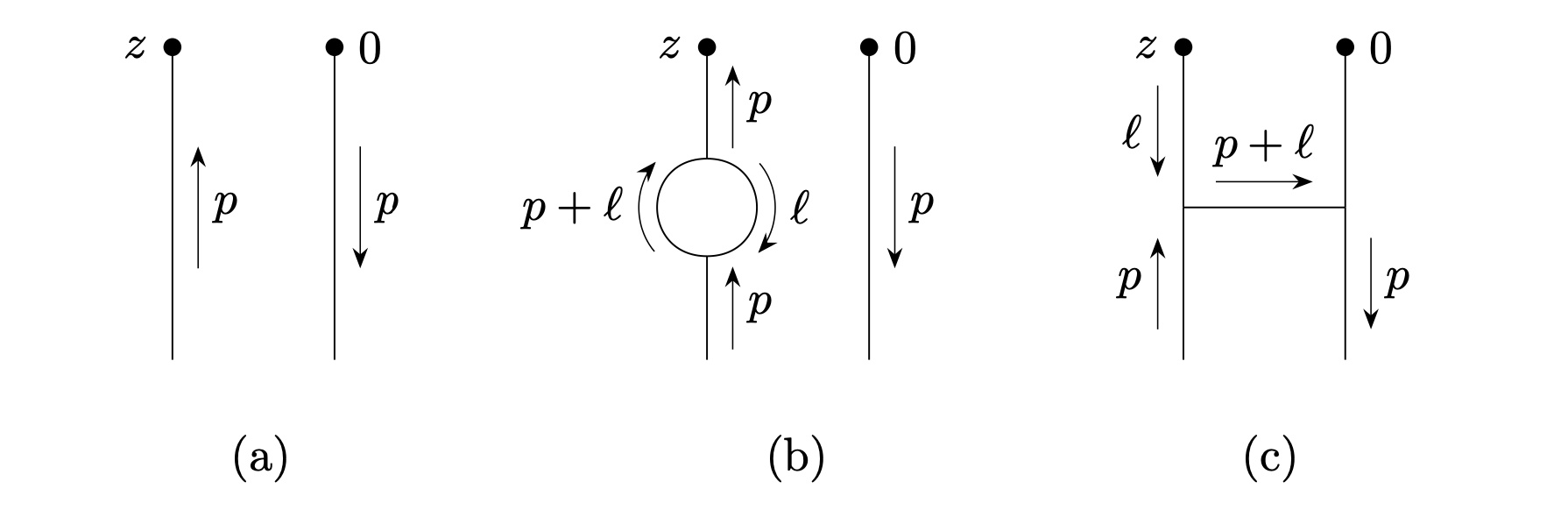
At tree-level, as shown in diagram (a), the matrix element only depends on $\nu$ ,

\displaystyle\widehat{\mathcal{M}}_{a}(\nu,z^{2})=\exp[-ip\cdot z]=\exp[-i\nu]=\widehat{\mathcal{M}}^{(0)}(\nu,0)\,.

Note that there is no difference between the light-cone and the Euclidean expression at tree level. In both cases the result only depends on the variable $\nu$ .

For a light-cone separation, $z^{2}=0$ , the bilinear at one-loop is logarithmically divergent. The renormalized matrix element is

	$\displaystyle\widehat{\mathcal{M}}_{R}\left(\nu;\mu^{2}\right)$	$\displaystyle=\left[1+\frac{\alpha}{6}\left(\log\frac{m^{2}}{\mu^{2}}+b\right)\right]\widehat{\mathcal{M}}^{(0)}\left(\nu,0\right)$		(5)
		$\displaystyle+\alpha\,\int_{0}^{1}dx\,\left(1-x\right)\,\log\frac{\mu^{2}}{m^{2}\left(1-x+x^{2}\right)}\widehat{\mathcal{M}}^{(0)}\left(x\nu,0\right)\,,$		(6)

where the one-loop corrections are proportional to the coupling $\alpha=\lambda^{2}/(64\pi^{3})$ . The multiplicative renormalization in the first line is the usual renormalization of the field, which appears in diagram (b). The convolution in the second line comes from diagram (c) in Fig. 3 and is the typical divergence that appears when such bilinears are concerned. Note that we have suppressed the dependence on $z^{2}$ since in the light-cone case we always have $z^{2}=0$ . The renormalized light-cone matrix element is the quantity that is directly related to the PDF.

For a Euclidean separation, $z^{2}=-z_{3}^{2}$ , the finite value of $z^{2}$ acts as a regulator and the one-loop calculation is finite after the usual renormalization of the field $\phi$ ,

	$\displaystyle\widehat{\mathcal{M}}_{R}\left(\nu,z_{3}^{2};\mu^{2}\right)$	$\displaystyle=\left[1+\frac{\alpha}{6}\left(\log\frac{m^{2}}{\mu^{2}}+b\right)\right]\widehat{\mathcal{M}}^{(0)}\left(\nu,0\right)$		(7)
		$\displaystyle~+\alpha\int_{0}^{1}dx\,\left(1-x\right)\,2K_{0}\left(mz_{3}\right)\widehat{\mathcal{M}}^{(0)}\left(x\nu,0\right)\,,$		(8)

where $K_{0}$ is a Bessel function, which is singular only at the origin $z_{3}=0$ .

3.2 Factorization

In order to obtain a factorization theorem, we expand the expression for the Euclidean correlator for $mz_{3}\ll 1$ ,

\displaystyle 2K_{0}\left(Mz_{3}\right)=-\log\left(m^{2}z_{3}^{2}\right)+2\log\left(2e^{-{}_{E}}\right)+\mathcal{O}\left(m^{2}z_{3}^{2}\right)\,.

We see explicitly that the function in the convolution is IR-divergent when $m\to 0$ . However, this divergence matches exactly the divergence in the convolution for the light-cone quantity. When relating the two renormalized expressions, the dependence on $m^{2}$ cancels and we obtain a relation that is IR-finite, as required in a factorization theorem. By inverting the relation between the light-cone renormalized correlator and the renormalized PDF $f_{r}$ , we can write

		$\displaystyle\widehat{\mathcal{M}}_{R}\left(\nu,-z_{3}^{2};\,\mu^{2}\right)=\int_{-1}^{1}d\xi\,\tilde{C}\left(\xi\nu,\mu^{2}z_{3}^{2}\right)\hat{f}_{R}\left(\xi,\mu^{2}\right)+O(m^{2}z_{3}^{2})$		(9)
		$\displaystyle\tilde{C}\left(\xi\nu,\mu^{2}z_{3}^{2}\right)=e^{i\xi\nu}-\alpha\int_{0}^{1}dx\,\left(1-x\right)\log\left(\mu^{2}z_{3}^{2}\frac{e^{2{}_{E}}}{4}\right)e^{ix\xi\nu}\,.$		(10)

The left-hand side of this equation is a Euclidean correlator, which can be computed using standard techniques in Monte Carlo simulations of QCD. The right-hand side is a convolution that involves the PDF as defined from the light-cone correlator. It is interesting to notice that the dependence on $z^{2}$ only appears at $O(\alpha)$ . This is the equivalent of the well-known violations of Bjorken scaling in DIS. Note also that the factorization formula receives corrections that are powers of $mz_{3}$ , i.e. factorization works at small distances, with power suppressed corrections, just like in DIS, with small distances replacing large momentum transfer.

There are a multitude of lattice observables that have been defined starting from the Euclidean correlator in position space discussed here, see e.g. Ref. [8, 9] for recent reviews and exhaustive references. All of these lattice observables are related to light-cone correlators and therefore to PDFs following the steps outlined above. First the lattice quantities need to be properly renormalized and then the renormalized observable – extrapolated to the continuum limit – is matched to PDFs via some factorization theorem. After this procedure has been completed the lattice observables are exactly on the same footing as experimental observables, e.g. like the structure functions $F_{i}$ introduced above in the context of DIS [7, 10].

4 Bayesian Inverse Problems

Determining the PDF from a finite set of lattice data using Eq. (9) is a typical example of an inverse problem. Lattice simulations can provide a finite number of input points, which are used to constrain a function, i.e. an element of an infinite-dimensional space. Such problem is clearly ill-defined and the solution does depend on a number of assumptions that need to be made. The formulation of the problem is summarised as a sketch in the diagram in Fig. 4. We aim to determine a function $f$ , in this particular case a function of one real variable $x$ . The model space, denoted $\mathcal{M}$ in the figure, is an infinite-dimensional space. The data set $A$ is a dicrete set, each point in the data set is some functional of the function $f$ , $z=\mathcal{G}(f)$ . Clearly the system is underdetermined, since it would require an infinite amount of data in order to uniquely determine the function $f$ . A more constructive way to phrase the problem can be formulated in a Bayesian framework [11]. Our knowledge, or prejudice, about the function $f$ is encoded in some prior $p(f)$ , which is then updated using the dataset:

p(f|A)\propto p(A|f)p(f)\,,

(11)

where on the right-hand side we have introduced the likelihood function $p(A|f)$ . In principle one could try to work in infinite-dimensional spaces and define a probability measure. While this is a possibility, it is easier to reduce the problem by parametrizing the function $f$ and work with a probability density in the finite-dimensional space of the parameters that define the model. Clearly the choice of the parametrization induces a bias that needs to be taken into account.

Figure 4: Schematic representation of an inverse problem. On the left of the figure we see the space of data, with some dataset

A

. On the right we have the space of measurable functions

\mathcal{M}(\mathcal{X},\mathcal{Y})

and the subset

\mathcal{F}

that we explore with a given parametrization.

4.1 NNPDF fits of lattice data

As explained in the previous section, lattice data are on the same footing as experimental input into PDFs fits. In a series of papers, some of the lattice data have been incorporated in the general fitting framework developed by the NNPDF collaboration [5, 6]. It is worthwhile to emphasise that the lattice data are handled like any other dataset in NNPDF, with no need to adjust the methodology. The only input needed is a robust estimate of the statistical covariance and the systematic errors. This is modeled by considering the data, $z$ , as stochastic variables distributed according to a multi-dimensional Gaussian distribution, centred at the value of the experimental measurement $Z$ , with a covariance $C$ , which we denote as

z\sim\mathcal{N}(Z,C)\,.

(12)

Parametrization

In the NNPDF formalism, the parametrization of the function $f$ is provided by neural networks, see Ref. [12] for the details of the latest implementation. A sufficiently large architecture provides a parametrization that is flexible enough to minize the functional bias. We denote the neural net parametrization as $g[\theta]$ , where $\theta$ is the set of parameters (biases and weights of the neural network).

Posterior Distribution.

The posterior distribution in the space of functions – i.e. in the space of functions that are parametrized by the neural networks – is described by a Monte Carlo set of replicas. The replicas implement a bootstrap propagation of the statistical fluctuations of data into the space of functions [13]. Each replica $z^{(k)}$ is obtained by generating a set of pseudo-data,

z^{(k)}=Z+\varepsilon^{(k)},~~k=1,\ldots N_{\mathrm{rep}}\,,

(13)

where $\varepsilon^{(k)}$ are distributed according to $\mathcal{N}(0,C)$ .

The set of replicas yields an ensemble of pseudo-data that reproduces the statistical distribution of the experimental data as encoded in the covariance matrix. For each replica, we perform a fit, i.e. we minimize a loss function, subject to constraints ¹¹ 1 The details of the training procedure are very important, but beyond the scope of these proceedings. We advise the interested reader to scrutinise the algorithm with great care, and refer them to the detailed explanations in Ref. [12].

	$\displaystyle{\chi^{2}}^{(k)}[\theta]$	$\displaystyle=\frac{1}{N_{\mathrm{dat}}}\sum_{ij}\left(g[\theta]^{(k)}-z^{(k)}\right)_{i}C^{-1}_{ij}\left(g[\theta]^{(k)}-z^{(k)}\right)_{j}+\mathrm{priors}\,,$		(14)
	$\displaystyle\theta^{(k)}$	$\displaystyle=\arg\min_{\theta}{\chi^{2}}^{(k)}[\theta]\,.$		(15)

Hence for each replica, we obtain a parametrization of the PDFs. This set of fitted parameters, $\left\{\theta^{(k)};k=1,\ldots,N_{\mathrm{rep}}\right\}$ , yields the desired posterior distribution in the space of functions. Note that this ensemble of replicas is an example of importance sampling of the posterior distribution in the space of functions parametrized by the neural networks.

Results of the fits to lattice data were presented in Refs. [5, 7]. A few examples are reported in Fig. 5 and 6. It is important to remark that the lattice error in these analysis is dominated by systematic errors.

Figure 5: PDFs extracted from lattice data using the NNPDF methodology. Results from Ref. [5]. The NNPDF fit to experimental data is shown in blue for comparison.

Despite the large errors, it is remarkable that a fairly small number of lattice data points provides a powerful constraint for the PDFs. It is clear that improved lattice simulations, with better control of systematic errors, could target the kinematical regions were the current uncertainties are large and have a significant impact.

5 Recent fits

Since the analyses in Refs. [5, 7], a large number of new simulations have appeared that have measured a broader variety of observables, and have improved both the statistical and systematic errors. These more recent simulations have also focused on helicity distributions, TMDs and GDPs, which are less precisely determined from fits to experimental data. These are areas where the lattice simulations are most likely to have a lasting impact. We do not have time to make an exhaustive review of contemporary results, for which we refer the reader to the recent proceedings of the Lattice conference [9]. In order to entice the audience, we report here a few results from recent publications. This is not an exhaustive list of result, but does give an idea of the potential for lattice QCD.

Unpolarised Gluon.

The HadStruc collaboration has performed a careful study of the unpolarised gluon distribution [14]. The study is interesting in many respects. In particular, the study takes into account the mixing of the gluon and the singlet bilinears under renormalization and introduces a new parametrization of the PDFs for their fits. The result is reported here in Fig. 7. Note that the pion mass in this work is still relatively large, $m_{\pi}\simeq 358~\mathrm{MeV}$ .

Another Unpolarized Gluon.

An independent determination of the unpolarised gluon distribution is presented in Ref. [15]. Despite the fact that a wider range of pion masses is explored, there are still systematic discrepancies between these determinations and the fits to experimental data, which deserve to be clarified. It would be interesting to perform a combined analysis of these results using the NNPDF methodology as explained in the previous Section. These determinations are the benchmarks that the lattice results need to satisfy in order to show that systematic errors are under control. Results are shown in Fig. 8.

Helicity and Transversity.

Ref. [16] is one example of a study that goes beyond the unpolarized distributions and addresses the determination of helicity and transversity parton distributions. These distributions are less constrained by experimental data, so that the impact of lattice simulations here is likely to be highly significant. Results are reported in Fig. 9.

6 Conclusion

Since the original work in Ref. [1], there has been a momentous activity in the lattice community in order to extract PDFs from numerical simulations of lattice QCD. Following a series of well-founded criticisms in Refs. [17, 18] the theoretical status of these studies has been carefully examined, and it is now clear that lattice data in Euclidean spacetime can be related to light-cone PDFs by factorization theorems after the lattice observables have been properly renormalized and extrapolated to the continuum limit.

In this respect, lattice data can be treated exactly like any other experimental data. The extraction of the PDFs requires the solution of an ill-defined inverse problem, whose result depends on the choice of priors. This is a delicate point, which needs to be analysed with great care. A Bayesian formulation facilitates the explicit formulation of the assumptions underlying the prior disribution. Having clarified the prior, the posterior distribution is given by Bayes theorem, and can be sampled e.g. by Monte Carlo methods as suggested in the NNPDF approach.

As the high-energy physics community is driven towards precision analyses at hadronic colliders, a faithful determination of the errors on the Parton Distribution Functions becomes increasingly important. We expect to see significant progress in this area, especially from the synergy of different approaches.

Acknowledgements

LDD is grateful to the collaborators who were involved in the studies used for these proceedings. T Giani and C Monahan contributed significantly to shaping the author’s understanding of the theoretical issues.

Funding information

LDD is supported by the U.K. Science and Technology Facility Council (STFC) grant ST/P000630/1.

References

[1] X. Ji, Parton physics on a euclidean lattice, Phys. Rev. Lett. 110, 262002 (2013), 10.1103/PhysRevLett.110.262002.
[2] J. C. Collins, INTRINSIC TRANSVERSE MOMENTUM. 1. NONGAUGE THEORIES, Phys. Rev. D 21, 2962 (1980), 10.1103/PhysRevD.21.2962.
[3] D. J. Gross and S. B. Treiman, Light-cone structure of current commutators in the gluon-quark model, Phys. Rev. D 4, 1059 (1971), 10.1103/PhysRevD.4.1059.
[4] H. Georgi and H. D. Politzer, Electroproduction scaling in an asymptotically free theory of strong interactions, Phys. Rev. D 9, 416 (1974), 10.1103/PhysRevD.9.416.
[5] K. Cichy, L. Del Debbio and T. Giani, Parton distributions from lattice data: the nonsinglet case, JHEP 10, 137 (2019), 10.1007/JHEP10(2019)137, 1907.06037.
[6] L. Del Debbio, T. Giani, J. Karpie, K. Orginos, A. Radyushkin and S. Zafeiropoulos, Neural-network analysis of Parton Distribution Functions from Ioffe-time pseudodistributions, JHEP 02, 138 (2021), 10.1007/JHEP02(2021)138, 2010.03996.
[7] L. Del Debbio, T. Giani and C. J. Monahan, Notes on lattice observables for parton distributions: nongauge theories, JHEP 09, 021 (2020), 10.1007/JHEP09(2020)021, 2007.02131.
[8] K. Cichy, Overview of lattice calculations of the x-dependence of PDFs, GPDs and TMDs, EPJ Web Conf. 258, 01005 (2022), 10.1051/epjconf/202225801005, 2111.04552.
[9] A. Scapellato, C. Alexandrou, K. Cichy, M. Constantinou, K. Hadjiyiannakou, K. Jansen and F. Steffens, Generalized parton distributions of the proton from lattice QCD, PoS LATTICE2021, 129 (2022), 10.22323/1.396.0129, 2111.03226.
[10] C. Monahan, Recent Developments in $x$ -dependent Structure Calculations, PoS LATTICE2018, 018 (2018), 10.22323/1.334.0018, 1811.00678.
[11] L. Del Debbio, T. Giani and M. Wilson, Bayesian approach to inverse problems: an application to NNPDF closure testing, Eur. Phys. J. C 82(4), 330 (2022), 10.1140/epjc/s10052-022-10297-x, 2111.05787.
[12] R. D. Ball et al., The path to proton structure at 1% accuracy, Eur. Phys. J. C 82(5), 428 (2022), 10.1140/epjc/s10052-022-10328-7, 2109.02653.
[13] B. Efron and R. J. Tibshirani, An Introduction to the Bootstrap, No. 57 in Monographs on Statistics and Applied Probability. Chapman & Hall/CRC, Boca Raton, Florida, USA (1993).
[14] T. Khan, R. S. Sufian, J. Karpie, C. J. Monahan, C. Egerer, B. Joó, W. Morris, K. Orginos, A. Radyushkin, D. G. Richards, E. Romero and S. Z. and, Unpolarized gluon distribution in the nucleon from lattice quantum chromodynamics, Physical Review D 104(9) (2021), 10.1103/physrevd.104.094516.
[15] Z. Fan, R. Zhang and H.-W. Lin, Nucleon gluon distribution function from 2 + 1 + 1-flavor lattice QCD, International Journal of Modern Physics A 36(13), 2150080 (2021), 10.1142/s0217751x21500809.
[16] C. Alexandrou, M. Constantinou, K. Hadjiyiannakou, K. Jansen and F. Manigrasso, Flavor decomposition for the proton unpolarized, helicity and transversity parton distribution functions, PoS LATTICE2021, 231 (2022), 10.22323/1.396.0231.
[17] G. C. Rossi and M. Testa, Note on lattice regularization and equal-time correlators for parton distribution functions, Phys. Rev. D 96(1), 014507 (2017), 10.1103/PhysRevD.96.014507, 1706.04428.
[18] G. Rossi and M. Testa, Euclidean versus Minkowski short distance, Phys. Rev. D 98(5), 054028 (2018), 10.1103/PhysRevD.98.054028, 1806.00808.