Topology-based Approximations for Contingency Constraints in Power Transmission NetworksJournal: International Journal of Electrical Power & Energy Systems
Abstract
It is crucial for maintaining the security of supply that transmission networks continue to operate even if a single line fails. Modeling security in power system capacity expansion problems introduces many extra constraints if all possible outages are accounted for, which leads to a high computational burden. Typical approaches to avoid this burden consider only a subset of possible outages relevant to a given dispatch situation. However, this relies on knowing the dispatch situation beforehand, and it is not suitable for investment optimization problems where the generation fleet is not known in advance. In this paper, we introduce a heuristic approach to model the fully secured feasible space using a smaller number of constraints in a way that only depends on the topology of transmission networks. In our proposed approach, the network’s security is modelled by comparing the polytope of the feasible space of nodal net power obtained from the security-constrained linearized AC optimal power flow problem. To approximate this polytope, a buffer capacity factor is defined for transmission lines in the secure case, thereby avoiding the introduction of many additional constraints. In this way, three approaches are introduced for obtaining a buffer capacity factor consisting of approximate, robust and line-specific approaches. Finally, the performance of our proposed approaches is assessed in different scales of transmission networks for determining the proposed buffer capacity factors, contingency analysis and economic evaluation. Moreover, we find that our proposed heuristics provide excellent approximations of the fully secured solutions with a much lower computational burden.
Keywords:
Linear optimal power flow , polytope , power system , reliability , security , transmission network.1 Introduction
1.1 Motivation
Security and reliability are defined as two of the most important goals of power systems to supply power demand continuously [1]. Thus, criteria have been introduced to retain the power system in a secure state when a single outage of power system components occurs [2]. Conventionally, security is modelled by many extra constraints to account for all outages, which leads to a high computational burden, even when the flow physics is linearized (a common approach for operational and capacity expansion problems). Typical approaches to avoid this burden are to consider only a subset of possible outages which are relevant for a given dispatch situation, iteratively adding the outage constraints until the network can be demonstrated by experimentation to be secure [3]. This approach depends on the dispatch situation and is unsuitable for investment optimization, where many dispatch situations are considered simultaneously and the generation is not known in advance. In the following section we summarise different approaches in the literature for modelling security constraints, so-called security-constrained linear optimal power flow (SCLOPF), to guarantee the power grid’s reliability and prevent line overloading and cascading failures in the system.
1.2 Related Works
Authors in [2, 4] presented how the current injection method retains the power system’s security in the optimal power flow problem by compensating power flow of the failed line based on injecting the virtual currents to prevent overloading in rest of the lines in the transmission network. Authors in [5] presented a mixed-integer program for the linearized AC optimal dispatch problem with transmission switching considering constraints. In [5], it has been evaluated how transmission switching can keep the security of the power system based on criteria. The transmission switching problem was also considered by authors in [6, 7]. A joint unit commitment and transmission switching problem considering constraints has been presented in [6]. A bi-level stochastic optimal switching model has been introduced for determining line switching strategy considering limitations in [7]. A preventive SCOPF problem has been proposed in [8] where authors assessed the performance of their proposed model in planning and operation problems of the power system. In the preventative SCOPF problems, the proposed problem consists of decision-making variables which are feasible for both pre-contingency (before single line outages) and post-contingency (after single line outages), simultaneously [9]. Ref. [10] proposed a risk-based decomposed model for contingencies in the power system. In [11], contingencies relaxation has been proposed. Authors in [12] presented a security-constrained multi-objective optimal power flow method considering security constraints. Ref. [13] proposed a mixed-integer programming model for linear optimal power flow considering conditions for preventing cascading failures in the power network. In [14], an algorithm has been proposed for reducing the constraints introduced by contingency scenarios of the SCOPF problem and finding the feasible space for nodal power injected based on a geometric algorithm. In [15], authors introduced an optimal topology control model considering constraints in the power systems. In [16], an umbrella constraint discovery problem has been introduced where the SCOPF problem is approximated by the linearised AC power flow. Authors in [17] proposed a framework for modeling zonal electricity markets and developed cutting-plane algorithms for considering security conditions.
1.3 Contributions
Although various models have been introduced in the literature to model security conditions in different applications of power systems, most of them are dependent on properties of components of the system, e.g. generators and loads, which increases the computational burden beyond what is solvable in reasonable time in the context of multi-period capacity expansion models. Moreover, there exist numerous alternative approaches with regards to contingency conditions in light of new technologies such as large-scale energy storage systems, e.g. batteries, that can be placed at the connecting nodes of transmission lines outage which can compensate as virtual lines for some time. In this paper, we present a topology-based security method for transmission line outages in a preventive SCOPF problem that can be applied in power system expansion problems. In other words, the power system’s security is solely studied based on the topology of the transmission network without relying on information about generators, loads and energy storage systems. Thus, this paper proposes a heuristic model for security constraints of the transmission grid by adding buffer capacity factor for transmission lines. In this way, we propose three heuristic approaches, consisting of robust, approximate and line-specific, without adding constraints for every single line outage. Our proposed models for security constraints are based on a secured linear optimal power flow formulation by adding a buffer capacity factor for each transmission line. For instance, the loading of a line may be limited to 70% of its real thermal capacity as an industry-standard [18, 19]. This way, the remaining 30% of the thermal capacity is kept as a reserve to guarantee security and reliability if another line fails [20]. However, the approximation has never been justified or shown to be robust, nor have line-specific factors been developed. Using a buffer capacity factor on the line capacities instead of the full set of constraints saves many heavy constraints and non-zero values in the constraint matrix. However, a price is paid for the lower computational burden as the heuristic approaches presented herein may be too optimistic or too conservative. The main contributions of this paper can be summarized as follows:
- 1.
We propose a heuristic approach for security constraints of the transmission power grid based on adding a buffer capacity factor for transmission lines that dramatically reduces number of necessary constraints.
- 2.
We investigate three approaches to find the buffer capacity factor for all or individual transmission lines.
- 3.
The performance of the fully secured network is compared with our proposed heuristic approaches.
- 4.
A sensitivity analysis of the proposed approaches is performed in different network topologies and German transmission networks.
The rest of this paper is organized as follows. Section 2 presents the problem formulation for the linearized AC optimal power flow problem under security constraints. In Section 3, our heuristic approaches to model secure network are introduced. Then, the simulation results are discussed in Section 4. Finally, our findings are summarised in Section 5.
2 Problem Formulation
2.1 Linearized AC Optimal Power Flow Problem
We consider the linearized AC optimal power flow (LOPF) problem that seeks to minimize the operational cost of generator dispatch under network constraints with fixed capacities. Nonlinear and non-convex formulations of power flow have not been considered in this paper because they cannot be solved within reasonable time in the context of large capacity planning problems. The problem is classified as a linear problem (LP) and no capacity expansion of generation, storage or transmission infrastructure is assumed. The objective function for the LOPF problem is given by (1).
| (1) |
where represents operation cost for generator at time . This way, represents the dispatched power of generator at time . The LOPF problem is constrained by physical equations and constraints which are presented in the following. Eq. (2) presents the balancing constraint based on Kirchhoff’s Current Law (KCL) requiring matching generation and demand at bus and time
| (2) |
where maps generator at bus . In other words, if generator is located at bus , otherwise . Besides, represents electricity demand at bus and time , and states power flow in line and time . Moreover, represents the incidence matrix between buses and lines as represented by (3)
| (3) |
Moreover, maximum and minimum limitations of dispatched power of generators are expressed by (4)
| (4) |
where represents the time-dependent potential of power generation for generator at time . Also, Eq. (5) states the constraint for avoiding emission exceeds a desired target level.
| (5) |
where is the specific emission of the fuel, is the generator efficiency, and is a fraction of the emissions in electricity [21].
2.2 Power Flow Constraints
In this section, nodal and line-specific power flow equations and constraints of the LOPF problem are represented. Power nodal balancing is one of the fundamental equations in the power system. In this paper, power loss is ignored for simplicity. Then, we obtain
| (6) |
where , and it represents net power injection at bus and time . Thus, positive (negative) value of presents network generation (load). Here, bus is chosen as a slack bus in the grid. In other words, are independent values and is the dependent value at each time snapshot. Authors in [22, 23, 24, 25] present the relation between power flow and nodal net power is given by (7)
| (7) |
where represents power transfer distribution factor (PTDF) between line and bus which is given by . Moreover, is a diagonal matrix of branch susceptance as it arrays are given by (8)
| (8) |
where is a reactance for line . Moreover, is a pseudo-inverse matrix of , as nodal susceptance matrix, which is obtained by . Thus, as is assumed as a slack bus, then . Maximum and minimum constraints of power flow are represented in (9)
| (9) |
where is the capacity of line . To model the secure network, it is necessary to define the secure network. The secure network is only secure as long as there is no line outage. According to security conditions, Eq. (10) is obtained based on (7) and (9)
| (10) |
In this way, independent nodal net powers () make the dimensional space at each time snapshot based on (10). In other words, at time , Eq. (10) constrains the –dimensional polytope with at most faces where is number of transmission lines in the network. We define this as the secure polytope .
2.3 Security Constraints
In this section, security constraints are presented that guarantee no overloading occurs in transmission lines if there is a single line outage ( criteria). In this way, if line fails, the flow in line at time after the outage of line () is related to the flows before the line outage in lines () and () based on the line outage distribution factor (LODF) represented in Eq. (11) [26]. Based on Eqs. (7) and (11), Eq. (12) is obtained [26]
| (11) | |||
| (12) |
where the and matrices are model coefficients and calculated before outage of line . Moreover is calculated according to Refs. [26, 27, 28] by Eq. (13)
| (13) |
where in case of . If there is an outage in one line (e.g. line fails), the power flow in lines after a single line outage is limited their corresponding thermal capacity which is given by (14)
| (14) |
Additionally, according to (13) and (14), Eq. (2.3) is obtained:
| (15) |
Thus, for a fully secured network, both Eqs. (10) and (2.3) must hold. This adds constraints from Eq. (2.3) to the constraints from Eq. (10) ( secure network) at each time snapshot. In this way, at time , the fully secured network can be represented by an –dimensional polytope consisting of constraints which is often computationally infeasible for large networks that consider a wide range of operating conditions. Thus, an approximation approach is needed to model security conditions for large networks. Our proposed heuristic methods are described in the following section.
3 Methodology
In our proposed methodology, we approximate the shape of the secure polytope by taking the secure polytope and introducing buffer capacity factors for each line to constrain it further. In this approach, we modify Eq. (9) to:
| (16) |
where represents buffer capacity factor for line which is between and , and it expresses the share of line nominal capacity that can be used. Thus, we define a new –dimensional polytope with at most faces in the space of possible nodal net powers. By definition, it is a subset of the secure polytope as long as for all lines.
3.1 Proposed heuristic approaches
We present three different approaches – consisting of robust, approximate, and line-specific – to choose the buffer capacity factors to get the best match between the polytope and the polytope (). While the same buffer capacity factor is allocated for all lines in robust and approximate approaches, the specific amount of buffer capacity factors are determined for each line in the line-specific approach. Additionally, while is entirely inside the in the robust and line-specific approaches, is not entirely inside the in the approximate approach and the volume of is equal to the volume of the in the approximate one. For contracting , firstly, we must shape and polytope of each single line failure scenario of the network. In this way, and present the polytopes if only lines and are failed, respectively. Hence, represents the common space between and polytope of all single line failure scenario
| (17) |
3.1.1 Robust approach
The robust approach is the most conservative one. In this approach, the buffer capacity factor is the same for all lines , and is chosen so that the resulting polytope is entirely inside the polytope of the fully secured network, , as shown in Fig. 1. This guarantees that any nodal imbalance inside will always be secure. However, it may be over-constrained such that there are more cost-effective dispatch solutions outside that are still secure, i.e. there may be better solutions in the set .
3.1.2 Approximate approach
This approach also has the same buffer capacity factor for every line, , but now is chosen such that the resulting polytope has the same volume as the fully secured polytope , i.e. which is less constraining than the robust approach where . This means the feasible space is the same size as the polytope, in the hope that the economic dispatch is better approximated by having a larger feasible space than the conservative robust approach. Now, like the robust case, we may still have secure solutions that are outside , i.e. the set is non-trivial, but we may also have solutions in that are now no longer secure, i.e. the set is non-trivial. Since , we have that the volume of these two non-trivial spaces is equal as represented by Eq. 18. The step-by-step implementation diagram of our proposed robust and approximate approaches are illustrated in Fig. 1.
| (18) |
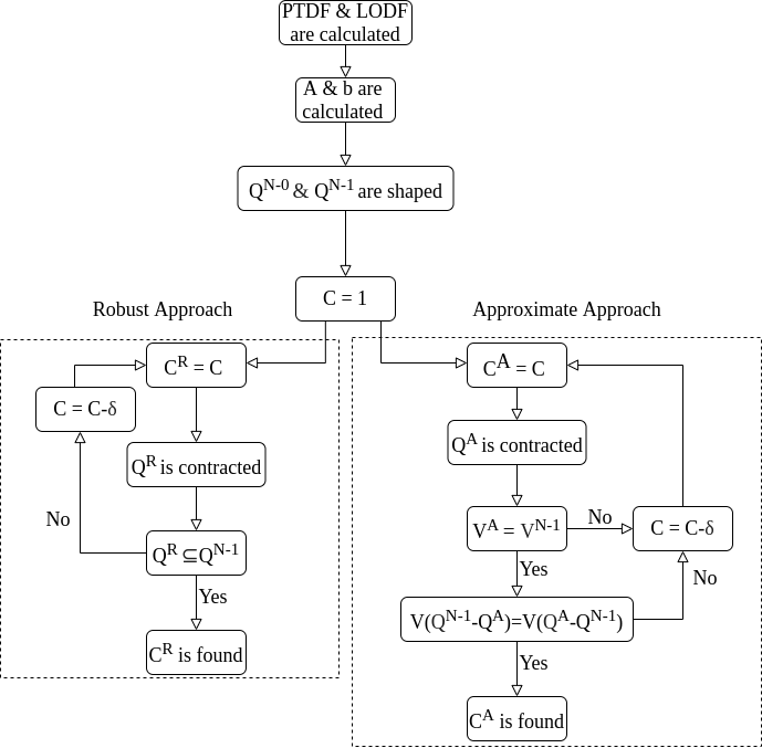
3.1.3 Line-specific approach
This approach builds on the robust approach by using the freedom to set the individual buffer capacity factor for each line, , in a way that keeps the overall polytope be inside while increasing the volume of the polytope. Thus, the maximum power transfer capacity for each line is determined based on the redundant capacity factor, , according to the Edmond-Karp algorithm [29, 30]. This way, if , it represents that power flow above the nominal capacity of line does not cause overloading in the rest of the lines in the network in the case of a single line outage of line . The redundant capacity factor for line is calculated based on the LOPF problem in the network after (i) removing line with start node and end node , (ii) adding power generation at node and load at node until one line becomes overloaded in the transmission network, and vice versa. Based on and , is determined iteratively as presented in Algorithm 1. The algorithm starts with the robust polytope, then increases for each line based on its corresponding , then incrementally reduces until the resulting polytope is robust, i.e. within .
3.2 Finding the volume of the polytope
As highlighted in Section 3.1.2, is found based on comparison between and . To determine the volume of the polytopes generated from our proposed approximate approach, a set of random samples is used, where is a –dimensional vector and represents for a single time. In this way, we use a quasi-random low-discrepancy series, e.g. the Halton sequence [31] to improve the convergence over pseudo-random sampling. Thus, the space in the bounding box of Eqs. (19) and (20) is covered more efficiently based on the polytope defined by Eq. (2.3).
| (19) | ||||
| (20) |
where and are the left-hand side and the right-hand side of Eq. (2.3), respectively. In this way, is a – dimensional vector and is a – dimensional matrix. Besides, and present lower and upper bounds of , respectively. Finally, samples constrained to (21) are selected for determining the volume of the polytope.
| (21) |
where is number of selected samples from and is total number of generated samples from in the bounding box and are not selected. This way, the volume of the polytope is calculated based on a hit-miss integration by Eq. (22):
| (22) |
where represents volume of the polytope.
3.3 Methodology for large numbers of buses
Our proposed heuristic approaches to find buffer capacity factors are based on estimating volumes of polytopes. It is noteworthy that estimating volumes of polytopes does not perform well on large-dimensional spaces because of the curse of dimensionality. To circumvent this problem, we apply the algorithms proposed in Section 3.1 on many smaller subsets of the buses separately. Moreover, a large number of subsets of buses is necessary for accurate results, which is a drawback for this method. For instance, for a network with 50 buses, we can take a group of buses, e.g. , buses and explore the –dimensional polytope defined by the space of possible dispatches of these buses, with all other buses having zero power dispatch. Thus, all line constraints are still active, and this is equivalent to only examining columns of the matrix in equation (21), but keeping all the rows that represent all the line constraints in the model as represented in (23).
| (23) |
In this way, the corresponding matrix for subset is given in (24).
| (24) |
Moreover, matrix is represented as consisting of for all subsets.
| (25) |
Geometrically this is equivalent to taking cross-sections of the polytope along particular subsets of dimensions while setting the coordinates of other dimensions to zero. By sampling many such subsets of nodes, corresponding to different cross-sections of the polytope, we can build information on the whole polytope. In this way, subsets can be selected by random selections or by clustering buses that are geographically close to each other using k-means algorithm [32]. In this way, and , which are represented as robust and approximate buffer capacity factors for cluster , respectively, are determined according to robust and approximate approaches described in Section 3.1. According to the definition of , we have
| (26) |
As presented in Eq. (26), the for the system must be the minimum of the line-specific buffer capacity factors of all lines. In this way, if we split the network to subsets, subset contains its corresponding lines and robust buffer capacity factor, , which is the minimum of line-specific buffer capacity factor for lines belonged to subset . Thus, the for the network split to several clusters can be defined as the minimum of robust buffer capacity of all subsets as represented in (27).
| (27) |
However, for determining , we need to figure out the relation between the buffer capacity factor and the volume of as compare to the volume of . In this paper, we define a criteria so-called volume ratio () for subset , which is given in (28). Regarding to the definition of the approximate approach in Section 3.1, one of the conditions for finding for the whole polytope is . In this way, we propose a criterion which is called the common volume ratio, , as represented in (29). Thus, is chosen to minimise the differences of the individual volume ratios from unity, see (30).
| (28) | |||
| (29) | |||
| (30) |
An alternative method for finding line-specific capacity factors () is proposed for large-scale networks based on the method for finding the robust subset factor (). In this way, the network is split to subsets in which buses and belong in the same subset if they connect directly with a transmission line. This way, matrix for the subset of line where is ended to buses as represented in (31)
| (31) |
In other words, each subset consists of only two buses that are connected with a transmission line and its line-specific buffer capacity factor, , equals the robust buffer capacity factor for the corresponding subset, , as seen in (32)
| (32) |


4 Simulation results
In this section, the performance of our proposed approaches to determine buffer capacity factors are studied. The LOPF problem is simulated in PyPSA [21]. The simulation results of our proposed approaches are evaluated in different test grids, including a 3-bus triangular network, some small-scale network topologies and a 50-bus Germany network as a large-scale network derived from PyPSA-Eur, an open-source model of the European electricity transmission system [33].
4.1 3-bus network
In this section, the performance of our proposed methodologies is studied in a 3-bus triangular network. Fig. 2a displays the scenario when there exist no line outage in the network. The scenarios are also illustrated in Fig. 2b where only one line outage has occurred in each of the scenarios. Assuming bus is a slack bus, there are two nodal net power injections ( and ) in the system. Thus, there exists a 2-dimensional polytope (so-called polygon) [34]. Fig. 3 demonstrates the feasible region between and in and scenarios, respectively. According to Fig. 3, feasible region between and for the fully secured network is illustrated in Fig. 4a. As mentioned in Section 3.1, we propose three approaches consisting of robust, approximate and line-specific approaches in this paper. Fig. 4c shows the polygons of feasible regions between and based on the approximate approach and fully secured network in a 3-bus triangular grid. The total volumes of both polygons, as well as the volumes of mismatched regions, are equal, as shown in Fig. 4c. On the other hand, the polygons of feasible regions between and based on the robust approach and fully secured network are illustrated in Fig. 4b. The polygon that came from the robust approach is completely covered by the polygon of fully secured network, and this is a reason why this approach is called robust. In other words, the feasible region of the robust approach is a subset of the feasible of the fully secured network, so (which is not a line-dependant factor) guarantees the reliability of the system in case of a single-line outage in the transmission network.
4.2 Small-scale networks

In this section, the performance of the proposed approaches for small-scale network topologies is evaluated European networks, which is derived from highly aggregated European transmission network, without cross-border connections with their neighborhoods as shown in Fig. 5. buffer capacity factor of each line obtained by the line-specific for small-scale European networks. Table 1 presents the values of and for small-scale networks. As seen in Table 1, is less than in all networks. Moreover, is around 0.7 for all small-scale networks. However, is not around 0.7 for all networks which is because of their specific topology. Table 1, for some of transmission lines are higher than . Additionally, the relation between the redundant capacity and buffer capacity factor is represented in Fig. . Thus, increment of is in line with the increment of . In other words, the lines with higher redundant capacity could have higher buffer capacity factor as seen in Fig. . Besides, the volume-in criteria (), which is defined in Eq. (33), obtained by approximate, robust and line-specific approaches, is displayed in Fig. 6.
| (33) |
According to Fig. 6, is maximum in the approximate approach. Moreover, of the line-specific approach is higher than the robust one presenting the effectiveness of the line-specific approach. However, note that even if the volume-in is high for the approximate approach, there will be parts of outside , making some solutions infeasible for .
| Network | Network | ||||
|---|---|---|---|---|---|
| (a) | 0.66 | 0.59 | (d) | 0.71 | 0.62 |
| (b) | 0.84 | 0.74 | (e) | 0.8 | 0.78 |
| (c) | 0.72 | 0.67 | (f) | 0.7 | 0.55 |
4.3 Large-scale network: German transmission system

In this section, the buffer capacity factor for the Germany network as a large-scale case study is found by our proposed methodology for a large number of buses as presented in Section 3.3. Fig. 7(a) displays 50-bus German transmission. Besides, Fig. 7(b) shows the total annual energy generation of energy carriers in the German transmission network. Additionally, a carbon emission reduction scenario is considered in this paper so that is just 10% of the electricity sector emissions in Germany in 1990. Table 2 presents buffer capacity factors for different subsets of the 50-bus Germany network based on the proposed clustering algorithm. The subsets represented in Table 2 are obtained by the k-means clustering algorithm and based on geographic proximity. As seen in Table 2, we assume 13 subsets for the 50-bus Germany network and determine and for each subset.
As seen in Table 2, for the 50-bus Germany network is which is obtained based on Eq. (26) which is the minimum of robust buffer capacity factor for each subset. On the other hand, Fig. 8(a) shows the impact of buffer capacity factor on in all subsets of the Germany network. As in k-means clustering, each bus belongs only to one cluster, we miss lines that cross clusters. In other words, the results came from k-means clustering do not guarantee security of our proposed robust approach. Thus, the robust buffer capacity factor is found by 100 random samples to cover all transmission lines in the transmission network, and is found which confirms outcomes presented by Table 2.
| Cluster | Cluster | ||||
|---|---|---|---|---|---|
| 0 | 0.62 | 0.77 | 7 | 0.66 | 0.75 |
| 1 | 0.67 | 0.76 | 8 | 0.66 | 0.77 |
| 2 | 0.73 | 0.81 | 9 | 0.65 | 0.73 |
| 3 | 0.8 | 0.81 | 10 | 0.71 | 0.83 |
| 4 | 0.71 | 0.75 | 11 | 0.78 | 0.85 |
| 5 | 0.59 | 0.68 | 12 | 0.61 | 0.73 |
| 6 | 0.77 | 0.83 | Total | 0.59 | 0.74 |
As seen in Fig. 8(a), increment of the buffer capacity factor increases for all subsets. However, their corresponding increment patterns are not the same. Moreover, for each subset is different as presented in Table 2. As shown in Fig. 8(b) and according to Eq. (30), there exists a minimum in the common volume criteria curve with buffer capacity equals as presented in Table 2. Fig. 9 illustrates the map of line-specific buffer capacity factors in Germany network which is calculated based on Eq. (32). According to Fig. 9, is in range of and for each line of the transmission network where lines with higher are more secure. Additionally, Fig. 10 shows the impact of buffer capacity factor on total number of secure transmission lines. As seen in Fig. 10, for all transmission lines are secured which proves equals for the German transmission network.

Additionally, the economic impact of the different buffer capacity factor approaches is studied in the German transmission network. In this analysis, operations are optimized for a full year of weather and load data for the 50 buses of the Germany network, assuming a generation fleet that yields a 90% CO2 reduction compared to 1990. This leads to a penetration of wind and solar power generation based on Fig. 7(b). Fig. 11(a) illustrates the impact of the buffer capacity factor on the yearly operational cost in Eq. (1), in the 50-bus Germany network. According to Fig. 11(a), increasing the amount of the buffer capacity factor decreases the operational cost of the system. Moreover, the operational cost of the system in the fully secured network is equal to the operational cost of the system with buffer capacity in the range of as seen in Fig. 11(a). As the approximate buffer capacity factor, , is found to be in Section 4.3, it can be concluded that the operational costs of the system in the fully secured network is close to the operational cost of the system with which confirms the intuitions from the industry that a buffer capacity factor of is suitable [20]. It is also noticeable that the close operational system costs do not necessarily imply that the operational results are the same. Moreover, Fig. 11(a) illustrates that the operational cost based on our proposed heuristic approach with the line-specific approach is higher than the operational cost in the fully secured case and less than the proposed robust approach. Furthermore, it has been found that operational costs of the system for a fully secured , approximate with line-specific buffer capacity factors, and approximate with approximate buffer capacity factor are very close. On the other hand, it is noteworthy that the approximate buffer capacity does not guarantee security of all transmission lines, whereas all lines are secured based on line-specific buffer capacity factor. Hence, the line-specific approach is the best approach among our proposed approaches to approximate the fully secured conditions in the network, while using uniform approximate buffer capacity factor can only provide approximation of operational costs of the fully secured .
| Computational | Memory | |
| time [Sec] | usage [MB] | |
| with uniform | 270 | 860 |
| buffer capacity factor | ||
| with line-specific | 326 | 860 |
| buffer capacity factor | ||
| fully secured | 3786 | 5582 |
According to Fig. 11(a), the robust case that guarantees no overloading is more expensive than the fully secured case since its feasible space is smaller. Moreover, the operational cost of the line-specific approach is lower than the robust one. Thus, while line-specific and robust approaches guarantee no overloading caused by a single-line outage in the network, the operational cost of the line-specific case is less than the robust one showing the benefit of the line-specific approach. Table 3 presents the computational time and memory usage of our proposed heuristic approaches with the uniform (approximate and robust) and line-specific buffer capacity factors in comparison with the fully secured problem. As seen in Table 3, the computational time and memory usage in our proposed method is significantly less than the fully secured case, which is because of fewer constraints in our proposed approximate case. Moreover, Fig. 11(b) shows total cases and snapshots where the transmission network is overloaded in at least one line for different buffer capacity factors. As shown in Fig. 11(b), there exists no overloading in the system for the buffer capacity factor less than (as has been obtained according to Fig. 10 and Table 2). In other words, Fig. 11(b) proves that the transmission network with a robust buffer capacity factor is guaranteed to be fully secured, i.e. no transmission line is ever overloaded.
5 Conclusion
In this paper, we have introduced a novel heuristic method for modeling the fully secured network considering contingencies based on the topology of the transmission network in the security-constrained linearized AC optimal power flow problem. To this end, the network’s secure feasible space has been determined by comparing the polytopes of the feasible region among nodal net power. Additionally, secure feasible regions have then been approximated using far fewer constraints by using the constraints with buffer capacity factors that have been obtained by line-specific, robust and approximate approaches to constrain the maximum loading of lines. The algorithms have been applied on smaller subsets and clusters of the buses to find line-specific, robust and approximate buffer capacity factors for networks with many buses. According to the simulations results of the test networks, it has been found that:
- 1.
The industry heuristic of buffer capacity is roughly suitable for the Germany network to provide fast results (since there are fewer constraints) while not producing significant overloading, and giving a system cost similar to the actual case.
- 2.
For absolute robustness while having fast results, you need to shrink the feasible space smaller than the true polytope, which leads to overestimation of the system cost. This can be mitigated by a novel line-specific buffer capacity, which better estimates the shape of the polytope while remaining robust.
- 3.
These speed-ups are particularly important when we include investment optimisation, which tends to increase the computational burden. Including fully secured constraints while optimising over a full year to dimension generation, storage, and transmission assets would be impossible, so these heuristics provide a good alternative that is still accurate.
In the future, maintaining security preventatively can be superseded with methods that use distributed flexibility to deal with contingencies like line failures reactively as they arise, thus allowing network assets to be fully used in regular operation.
Acknowledgement
This paper was conducted as part of the CoNDyNet2 project, which was supported by the German Federal Ministry of Education and Research under grant number 03EK3055E.
References
- [1] G. Schnyder, H. Glavitsch, Integrated security control using an optimal power flow and switching concepts, IEEE Transactions on Power Systems 3 (2) (1988) 782–790.
- [2] G. Glanzmann, G. Andersson, Incorporation of n-1 security into optimal power flow for facts control, in: 2006 IEEE PES Power Systems Conference and Exposition, IEEE, 2006, pp. 683–688.
- [3] D. A. Tejada-Arango, P. Sánchez-Martın, A. Ramos, Security constrained unit commitment using line outage distribution factors, IEEE Transactions on power systems 33 (1) (2017) 329–337.
- [4] G. Hug-Glanzmann, G. Andersson, N- 1 security in optimal power flow control applied to limited areas, IET generation, transmission & distribution 3 (2) (2009) 206–215.
- [5] K. W. Hedman, R. P. O’Neill, E. B. Fisher, S. S. Oren, Optimal transmission switching with contingency analysis, IEEE Transactions on Power Systems 24 (3) (2009) 1577–1586.
- [6] K. W. Hedman, M. C. Ferris, R. P. O’Neill, E. B. Fisher, S. S. Oren, Co-optimization of generation unit commitment and transmission switching with n-1 reliability, IEEE Transactions on Power Systems 25 (2) (2010) 1052–1063.
- [7] H. Zhang, H. Cheng, J. Zhang, J. Lu, C. Li, Stochastic optimal transmission switching considering n-1 security constraints, in: 2018 IEEE Power & Energy Society General Meeting (PESGM), IEEE, 2018, pp. 1–5.
- [8] F. Dong, L. Huang, B. P. Lam, X. Xu, Practical applications of preventive security constrained optimal power flow, in: 2012 IEEE Power and Energy Society General Meeting, IEEE, 2012, pp. 1–5.
- [9] V. H. Hinojosa, F. Gonzalez-Longatt, Preventive security-constrained dcopf formulation using power transmission distribution factors and line outage distribution factors, Energies 11 (6) (2018) 1497.
- [10] K. Karoui, H. Crisciu, A. Szekut, M. Stubbe, Large scale security constrained optimal power flow, in: 16th Power System Computation Conference, Glasgow Scotland, Citeseer, 2008, pp. 14–18.
- [11] F. Capitanescu, Approaches to obtain usable solutions for infeasible security-constrained optimal power flow problems due to conflicting contingencies, in: 2019 IEEE Milan PowerTech, IEEE, 2019, pp. 1–6.
- [12] Y. Li, Y. Li, Security-constrained multi-objective optimal power flow for a hybrid ac/vsc-mtdc system with lasso-based contingency filtering, IEEE Access (2019).
- [13] N. Fan, R. Chen, J.-P. Watson, N-1-1 contingency-constrained optimal power flow by interdiction methods, in: 2012 IEEE Power and Energy Society General Meeting, IEEE, 2012, pp. 1–6.
- [14] R. Weinhold, R. Mieth, Fast security-constrained optimal power flow through low-impact and redundancy screening, IEEE Transactions on Power Systems 35 (6) (2020) 4574–4584.
- [15] G. Poyrazoglu, H. Oh, Optimal topology control with physical power flow constraints and n-1 contingency criterion, IEEE Transactions on Power Systems 30 (6) (2015) 3063–3071.
- [16] A. J. Ardakani, F. Bouffard, Identification of umbrella constraints in dc-based security-constrained optimal power flow, IEEE Transactions on Power Systems 28 (4) (2013) 3924–3934.
- [17] I. Aravena, Q. Lete, A. Papavasiliou, Y. Smeers, Transmission capacity allocation in zonal electricity markets, Technical report, UCLouvain (2020).
- [18] T. Brown, P.-P. Schierhorn, E. Tröster, T. Ackermann, Optimising the european transmission system for 77% renewable electricity by 2030, IET Renewable Power Generation 10 (1) (2016) 3–9.
- [19] D. P. Schlachtberger, T. Brown, S. Schramm, M. Greiner, The benefits of cooperation in a highly renewable european electricity network, Energy 134 (2017) 469–481.
- [20]
M. Gathmann,
Mastering
power grid dynamics.
URL https://new.siemens.com/global/en/company/stories/energy/mastering-power-grid-dynamics.html - [21]
T. Brown, J. Hörsch, D. Schlachtberger,
PyPSA: Python for Power System
Analysis, Journal of Open Research Software 6 (4) (2018).
arXiv:1707.09913,
doi:10.5334/jors.188.
URL https://doi.org/10.5334/jors.188 - [22] A. J. Wood, B. F. Wollenberg, G. B. Sheblé, Power generation, operation, and control, John Wiley & Sons, 2013.
- [23] J. Hörsch, H. Ronellenfitsch, D. Witthaut, T. Brown, Linear optimal power flow using cycle flows, Electric Power Systems Research 158 (2018) 126–135.
- [24] V. Hinojosa, J. Velásquez, Improving the mathematical formulation of security-constrained generation capacity expansion planning using power transmission distribution factors and line outage distribution factors, Electric Power Systems Research 140 (2016) 391–400.
- [25] V. Hinojosa, F. Gonzalez-Longatt, Stochastic security-constrained generation expansion planning methodology based on a generalized line outage distribution factors, in: 2017 IEEE Manchester PowerTech, IEEE, 2017, pp. 1–6.
- [26] H. Ronellenfitsch, D. Manik, J. Hörsch, T. Brown, D. Witthaut, Dual theory of transmission line outages, IEEE Transactions on Power Systems 32 (5) (2017) 4060–4068.
- [27] T. Guler, G. Gross, M. Liu, Generalized line outage distribution factors, IEEE Transactions on Power systems 22 (2) (2007) 879–881.
- [28] J. Guo, Y. Fu, Z. Li, M. Shahidehpour, Direct calculation of line outage distribution factors, IEEE Transactions on Power Systems 24 (3) (2009) 1633–1634.
- [29] J. Edmonds, R. M. Karp, Theoretical improvements in algorithmic efficiency for network flow problems, Journal of the ACM (JACM) 19 (2) (1972) 248–264.
- [30] D. Witthaut, M. Rohden, X. Zhang, S. Hallerberg, M. Timme, Critical links and nonlocal rerouting in complex supply networks, Physical review letters 116 (13) (2016) 138701.
- [31] L. Kuipers, H. Niederreiter, Uniform distribution of sequences, Courier Corporation, 2012.
- [32] T. Kanungo, D. M. Mount, N. S. Netanyahu, C. D. Piatko, R. Silverman, A. Y. Wu, An efficient k-means clustering algorithm: Analysis and implementation, IEEE transactions on pattern analysis and machine intelligence 24 (7) (2002) 881–892.
- [33] J. Hörsch, F. Hofmann, D. Schlachtberger, T. Brown, Pypsa-eur: An open optimisation model of the european transmission system, Energy strategy reviews 22 (2018) 207–215.
- [34] C. D. Toth, J. O’Rourke, J. E. Goodman, Handbook of discrete and computational geometry, CRC press, 2017.