Abstract

NON COMMON PATH ABERRATIONS CORRECTION

jean-baptiste ruffio¹¹ 1 Institut Supérieur de l’aéronautique et de l’espace, ISAE-Supaéro, Toulouse, France ²² 2 Université Paul Sabatier, Toulouse III, France

Application of Electric Field Conjugation on SPHERE and use of Phase Diversity on the AOF.

master thesis
Adaptive Optics Department, ESO, Garching, Germany

Scientific Supervisor: Markus Kasper ³³ 3 Adaptive Optics Department, ESO, Garching, Germany
University Supervisor: Sébastien Massenot 1

august 2014 – version 1.0

Jean-Baptiste Ruffio: Non Common Path Aberrations Correction , Application of Electric Field Conjugation on SPHERE and use of Phase Diversity on the AOF., © august 2014

Abstract

The primary goal of this thesis was the correction of Non-Common-Path-Aberrations in the SPHERE instrument for helping it meeting its contrast requirements. SPHERE’s purpose is the search and characterization of giant exo-planets around nearby stars. The author implemented a method called Electric Field Conjugation that he tested in simulation as well as on the real system. A full week was booked in SPHERE schedule a few days before the second commissioning in June 2014. It gave the opportunity to the author to travel to the VLT in Chile and experiment directly on the system. The contrast gain objective of another order of magnitude in a medium-sized area has successfully been reached bringing SPHERE raw speckle contrast from about $10^{-6}$ to $10^{-7}$ . The algorithm has therefore proven its value and will be further investigated and hopefully automated by the SPHERE team based on the codes developed by the author. However it is important to keep in mind that Electric Field Conjugation is more effective for follow-up studies in order to improve the quality of the observations. Indeed the area for a good correction is very limited. It can’t be used for exo-planets discovery unless the corrected area is made big enough but the performance will be less.

Electric Field Conjugation is only one of the many algorithms for correcting speckles and that is why the author got interested in another project. ESO’s Adaptive Optics Facility is currently being tested on the ASSIST test bench at ESO headquarters in Garching, Germany. This bench suffers from a bad quality Point Spread Function and the goal of the author was to understand why an existing method called Phase Diversity couldn’t improve the Strehl Ratio. Therefore he implemented a new and more flexible code and performed a series of tests. The ASSIST test bench was indeed booked during a week in Mai 2014. After validating the code and exploring different parameters the AOF team got convinced that the problem was not coming from low order phase aberration that could be corrected using the Deformable Mirror and Phase Diversity. In average the performance of the author’s algorithm on ASSIST was an improvement of the Strehl Ratio of about $10\%$ from $60$ to $70\%$ with a peak at almost $80\%$ at a wavelength of $1.6\mu m$ .

In this world there is room for everyone. And the good earth is rich and can provide for everyone. The way of life can be free and beautiful, but we have lost the way. Greed has poisoned men’s souls, has barricaded the world with hate, has goose-stepped us into misery and bloodshed. We have developed speed, but we have shut ourselves in. Machinery that gives abundance has left us in want. Our knowledge has made us cynical. Our cleverness, hard and unkind. We think too much and feel too little. More than machinery we need humanity. More than cleverness we need kindness and gentleness. Without these qualities, life will be violent and all will be lost.

Hinkel The Great Dictator - Final Speech of the Barber,^†^†margin: Youtube link. ^†^†margin: Youtube link.

— Charlie Chaplin.

Acknowledgements

First I would like to thank my supervisor Markus Kasper for this opportunity to work in a great environment such as ESO. Few are the interns having the opportunity to travel to Chile and visit le Very Large Telescope. By the way thank you to Norbert Hubin who agreed to finance this trip. Despite the distance Markus made himself available for answering any of my questions and who knows how annoying I am.
Then big thanks to Johann Kolb who accepted my contribution to his project when I was getting low in tasks to do.
Thank you to Christophe Vérinaud for welcoming me in Grenoble and helping me understand Electric Field Conjugation.
Thank you to Bruce Macintosh for recommending me to Markus Kasper and therefore making this internship possible.
And I have to thank Anthony Berdeu for the skype-chat preventing me from working. Mh…Actually I might be the one preventing him from working!

Finally thank you to André Miede for developing and making available the template classicthesis used for this document. A real postcard has been sent to him as he wished.

\manualmark

ection]chapter

Acronyms

AOF: Adaptive Optics Facility
ASSIST: Adaptive Secondary Setup and Instrument Simulator
COFFEE: COronagraphic PHase diversitY
DOTF: Differential Optical Transfer Function
EFC: Electric Field Conjugation
EPICS: Exoplanet Imaging Camera and Spectrograph
FFREE: Fresnel-FRee Experiment for EPICS
ESO: European Southern Observatory
GALACSI: Ground Atmospheric Layer Adaptive Optics for Spectroscopic Imaging
GRAAL: GRound-layer Adaptive optics Assisted by Laser
HOT: High Order Testbench
IM: Interaction Matrix
IPAG: Institut de Planétologie et d’Astrophysique de Grenoble
IRDIS: Infra-Ref Dual-beam Imager and Spectrograph
ONERA: Office National d’Études et de Recherches Aérospatiales
PD: Phase Diversity
PSF: Point Spread Function
PSI: Phase Sorting Technique
RMS: Root-Mean-Square
SPHERE: Spectro-Polarimetric High-contrast Exoplanet REsearch
UT3: Unit Telescope 3
VLT: Very Large Telescope

^†^†margin: 1 Introduction

The Spectro-Polarimetric High-contrast Exoplanet REsearch (SPHERE) instrument has been installed at the Very Large Telescope (VLT) in spring 2014. SPHERE includes a very powerful Adaptive Optics for correcting the wavefront distortion due to the atmospheric turbulence. However even the best Adaptive Optics systems still suffer apparition of noise called speckles originating from defects inside the optical train and after the Adaptive Optics system. Methods have therefore been developed to measure the wavefront distortion using the science camera. A shape of the deformable mirror is inferred to suppress the speckles. One of this method is called Electric Field Conjugation (EFC). The goal of the Master Thesis is to implement it for SPHERE using Matlab. In addition of this main goal another phase aberration correction techniques was implement for the Adaptive Optics Facility which is a project of secondary Deformable Mirror for the VLT. This method is called Phase diversity and aims at improving the quality of the Point Spread Function by removing low order aberrations. This document first emphasizes the general context and the aims of the thesis in an introductory chapter. Then it is followed by one part for each the Phase Diversity and the Electric Field Conjugation method. These two parts are built in the same manner: first basic elements of theory are given, then simulated respectively experimental results are exposed. Besides there is one bibliographic section called State of the Art and a list of references per part. To finish almost every chapter has a paragraph emphasizing the author’s contributions.

The demonstrations of the methods even though very interesting have been pushed to the appendix. A week of tests for each instrument SPHERE and the AOF has been performed. The very essential of these tests has been exposed in the following. The complete set of tests for SPHERE is presented in the appendix while the complete tests for the AOF are available in a separate technical report.

Warning

The author acknowledge that the $30$ pages requirement of Université Paul Sabatier, Toulouse III, France is not formally fulfilled as the table of contents states $47$ . It is explained by the layout of this document which is very light with big margins and a lot of white pages for clarity. However it doesn’t contain more than $12$ thousand words which gives $26$ pages using a standard $500$ words pages with $11\text{pt}$ according to http://www.wordstopages.com/.

1 Context

Extrasolar planets or exo-planets are very faint objects orbiting very close to their host star. They are therefore very difficult to observe but thanks to technological and data processing techniques improvements it became one of the most dynamic research field in Astronomy. Nowadays the most common way to detect exo-planets is to use indirect methods. They are indirect because they consist in observing the different perturbations of the host star due to the presence of a close-orbiting body^†^†margin: For instance transits or radial velocity for the common ones ^†^†margin: For instance transits or radial velocity for the common ones . However for the past ten years a couple of exo-planets around nearby stars have been directly imaged opening a new era for detecting and characterizing exo-planets. The development of eXtreme ^†^†margin: Extreme means very efficient. ^†^†margin: Extreme means very efficient. Adaptive Optics systems have triggered the development of a new generation of instrument dedicated to exo-planets imaging. Direct imaging is briefly described in the following. The other methods short descriptions as well as their advantages and limitations can be found in Appendix 8.A.

Direct imaging allows one to get the light of the planet itself. Its great advantage is the possibility of characterizing the planet by studying the spectrum of its atmosphere for instance. Indirect methods will only provide with basic parameters like mass, size and orbital parameters.^†^†margin: Sometimes also a very low resolution spectrum… ^†^†margin: Sometimes also a very low resolution spectrum… Besides direct imaging is not constraint by the limitations inherent to indirect methods which need significant induced perturbations on the host star. The direct detection is limited by the separation power or resolution of the telescope and the brightness of the planet which determines a required contrast to achieve. The contrast is the ratio between the intensity of the star and the intensity of the planet. It is easier to detect bright planets far from the star. The ultimate goal of high contrast imaging is to observe an earth-like planet with evidence of life but it is not even sure that the next generation of 40 meters telescopes will suffice. Direct imaging instruments are usually coronagraphs with eXtreme Adaptive Optics. Coronagraphs are described in Section 9.D.2 and Adaptive Optics system in Appendix 9.C. Two such instruments have recently been built both on a eight meter class telescopes : SPHERE on the Very Large Telescope (VLT) and GPI on GEMINI-South.^†^†margin: SPHERE is European and GPI is American-Canadian ^†^†margin: SPHERE is European and GPI is American-Canadian

SPHERE

SPHERE stands for Spectro-Polarimetric High-contrast Exo-planet Research described in Beuzit et al. 2008 [3]. It is being commissioned at the VLT during this summer 2014. It includes three science paths: a differential infrared imager and spectrograph called IRDIS, an integral field spectrograph and a visible light polarimeter.

Gemini Planet Imager (GPI)

GPI described in Macintosh et al. 2006 [10] was a few months ahead and it has already begun its science phase at the Gemini south telescope. It is very similar to SPHERE but it possesses a single scientific instrument: a infrared Integral Field Spectrometer with a polarimetric mode. Figure 1 shows the first light image of an already known planet Beta Pictoris b.

Refer to caption — Figure 1: Gemini Planet Imager’s first light image of Beta Pictoris b, a planet orbiting the star Beta Pictoris. Source: www.gemini.edu.

2 Master Thesis

2.1 Motivations and Objectives

The purpose of the master thesis was to correct Non-Common-Path-Aberrations of optical instruments. The Non-Common-Path-Aberrations^†^†margin: For a description of the non-common-path see Section 9.C.3. ^†^†margin: For a description of the non-common-path see Section 9.C.3. are phase aberrations due to the optics defects but not seen by the wavefront sensor of the Adaptive Optics system. More particularly it was meant to be done on SPHERE. The method chosen for correcting these aberrations is Electric Field Conjugation and it will be described later on. However the author quickly realized that this would not keep him occupied for five months. At the mean time the Adaptive Optics Facility (AOF) was being tested on a bench called ASSIST in the laboratory of ESO in Garching. This bench suffered from a bad quality and unstable Point Spread Function measured by a relatively low Strehl Ratio^†^†margin: Low means $50-80\%$ . For more on Strehl Ratio see Appendix 9.B. ^†^†margin: Low means $50-80\%$ . For more on Strehl Ratio see Appendix 9.B. . A solution to improve Point Spread Functions is to apply a method called Phase Diversity. It is an algorithm for correcting Non-Common-Path-Aberrations. The algorithm used by ESO was developed by ONERA⁴⁴ 4 Office National d’Études et de Recherches Aérospatiales (ONERA) using IDL⁵⁵ 5 Interactive Data Language (IDL) and it didn’t give the expected results. The author took that opportunity to work on this other algorithm. The goal of the author was to help better understanding the ASSIST bench and try to improve the image quality or at least identify the causes. It went through coding a new algorithm on Matlab.

However the main goal of the thesis was still to work on SPHERE. In the framework of high-contrast imaging what determines the accuracy of an instrument is the contrast it is able to achieve. The contrast is indeed limited by the existence of random speckles in the image and it is not possible to detect planets fainter that the speckles themselves. The different causes for the speckles are first the atmospheric turbulence and then the optical aberrations. The Adaptive Optics deals with the main part of the atmospheric turbulence. The residual atmospheric speckles are short lived and randomly distributed so that a long exposure time makes them negligible. Indeed they average themselves with time forming a uniform background tending to zero relatively to the planet which doesn’t move and therefore strengthen its flux. At the end only what are called the quasi-static speckles are left. This speckles are constant on long time scales^†^†margin: Here long time scale means the exposure time which is the most critical. Longer time scales can be otherwise calibrated and shorted time scales are averaged like with the atmospheric speckles. ^†^†margin: Here long time scale means the exposure time which is the most critical. Longer time scales can be otherwise calibrated and shorted time scales are averaged like with the atmospheric speckles. so that long exposure makes them brighter in the same way as the planet. These are the speckles caused by optical aberrations in the instrument. The goal of Electric Field Conjugation is to correct for these aberrations and therefore improving the contrast. However the goal of the internship was less to reach a given contrast than to give preliminary results for validating the principles and therefore justifying the need of further investigations.

2.2 Methodology

The methodology was the same in both cases for the Phase Diversity as well as for the Electric Field Conjugation algorithm. The first step has been to get a deep understanding of the theory behind each method. In order to do so the author read the associated reference papers and made the demonstrations all over again^†^†margin: The demonstration was even improved for EFC. ^†^†margin: The demonstration was even improved for EFC. . The demonstration can be found in Appendix. Then simulation codes on Matlab were implemented to verify the overall principles and to perform some sensitivity studies. Both algorithms are based on a single Fourier Optics library of functions developed by the author for this occasion. Afterwards experiments were done on real systems which are respectively the AOF and SPHERE. To finish all the results were recorded in the present report and other documentations.

2.3 Means

The AOF is a future upgrade of the VLT UT4 which aims to create a adaptive telescope by replacing the secondary mirror by a deformable one. The AOF also includes several instruments optimized for this configuration. The AOF is currently being tested for two years 2014-2015 on a bench called ASSIST⁶⁶ 6 Adaptive Secondary Setup and Instrument Simulator (ASSIST) in Garching, Germany. ASSIST includes the Secondary Deformable Mirror and one of the two Adaptive Optics modules GRAAL⁷⁷ 7 GRound-layer Adaptive Optics Assisted by Laser (GRAAL) or GALACSI⁸⁸ 8 Ground Atmospheric Layer Adaptive Optics for Spectroscopic Imaging (GALACSI). The author was present when the first Adaptive Optics module GRAAL was tested. A full week from June $2^{th}$ to $7^{th}$ was dedicated to Phase Diversity tests with the author’s code.

Electric Field Conjugation was applied on the instrument IRDIS of SPHERE at UT3 of the VLT in Paranal, Chile. IRDIS means Infra-Red Dual-beam Imager and Spectrograph. IRDIS is one of the three instruments of SPHERE. The author had the opportunity to spend a week at the summit of Paranal between the $24^{th}$ and the $29^{th}$ of june 2014 for testing the method. This took place a week before the second commissioning of SPHERE. ^†^†margin: The overall stay in Chile was from June, 23 and July, 2. ^†^†margin: The overall stay in Chile was from June, 23 and July, 2. Besides the author spent a week from the April $19^{th}$ to $26^{th}$ at the Institut de Planétologie et d’Astrophysique de Grenoble (IPAG), Grenoble, France for preparing the experiment on a test bench called FFREE. FFREE stands for Fresnel-FREE Experiment for EPICS. However a week was to short for the author to really experiment on the bench. This visit was still a good opportunity to talk about the method with Christophe Vérinaud who actually already applied the method on FFREE.

3 State of the Art

There are a lot of different methods with different names for correcting non-common-path phase aberrations in regular or coronagraphic environments: EFC, COFFEE, PSI, DOTF…. However they are based on the same principle which is to create diversity in the phase for estimating the Electric Field from intensity measurements. The diversity indeed works as a sort of interferometer. Using the science camera to do the measurements allows one to correct for the Non-Common-Path-Aberrations as the same optical path is used for the science and for the correction. A list of references is given in Appendix 8.B^†^†margin: These references is in Appendix because the author read only the abstracts and don’t feel confortable about them. ^†^†margin: These references is in Appendix because the author read only the abstracts and don’t feel confortable about them. . Besides another bibliographical section is available for each part one Phase Diversity and one for Electric Field Conjugation.

The methods above should be applied before the measurements are made. However two post-processing methods are worth mentioning here because they are very efficient and widely used. Both methods are usually used in combination.

The first one is called Angular Differential Imaging (ADI) Marois et al. 2006 [13]. The principle of Angular Differential Imaging is to build a model of the speckles using a few sky-rotated images as shown in Figure 2. In practice the images are taken after disabling the sky rotation compensation of the telescope. The planet will then rotate around the star as the sky is rotating during the night while the speckles will remain constant in the image. The speckles model is then subtracted from the images and finally the rotated images are combined.

The second method called Spectral Differential Imaging also builds a model of the speckles. However this time it uses their wavelength dependency.^†^†margin: But the position of the planet is not wavelength dependent. ^†^†margin: But the position of the planet is not wavelength dependent. The speckles indeed follow the behaviour of the Point Spread Function which widen as the wavelength gets lower. The speckles can then be retrieved from radially scaled images taken at different wavelength. If the spectral range of the images is to limited for excluding the planet from the model it can also make use of spectral features in the planet not present in the star. For example the planets usually include methane in their atmosphere making them very faint compared to the star in the methane absorption band. Therefore one can subtract a scaled image at such wavelengths from another image where there isn’t methane dimming.

References

Aller-Carpentier [2011] Emmanuel Aller-Carpentier. Extreme Adaptive Optics system optimization for High Contrast Imaging with the high Order Test bench. PhD thesis, Universidad Autonoma de Madrid, 2011.
Batalha et al. [2013] Nathalie M. Batalha et al. Planetary candidates observed by kepler. iii. analysis of the first 16 months of data. The Astrophysical Journal. Supplement Series., 2013.
Beuzit et al. [2008] J.-L. Beuzit, M. Feldt, K. Dohlen, D. Mouillet, P. Puget, F. Wildi, L. Abe, J. Antichi, A. Baruffolo, P. Baudoz, A. Boccaletti, M. Carbillet, J. Charton, R. Claudi, M. Downing, C. Fabron, P. Feautrier, E. Fedrigo, T. Fusco, J.-L. Gach, R. Gratton, T. Henning, N. Hubin, F. Joos, M. Kasper, M. Langlois, R. Lenzen, C. Moutou, A. Pavlov, C. Petit, J. Pragt, P. Rabou, F. Rigal, R. Roelfsema, G. Rousset, M. Saisse, H.-M. Schmid, E. Stadler, C. Thalmann, M. Turatto, S. Udry, F. Vakili, and R. Waters. Sphere: a ’planet finder’ instrument for the vlt. In Society of Photo-Optical Instrumentation Engineers (SPIE) Conference Series, volume 7014 of Society of Photo-Optical Instrumentation Engineers (SPIE) Conference Series, July 2008. 10.1117/12.790120. URL http://adsabs.harvard.edu/abs/2008SPIE.7014E..18B.
Bordé and Traub [2006] Pascal J. Bordé and Wesley A. Traub. High-contrast imaging from space: Speckle nulling in a low aberration regime. Astrophysical Journal, 2006.
Born and Wolf [1980] Max Born and Emil Wolf. Principle of Optics. Cambridge University Press, 6 edition, 1980.
Cavarroc et al. [2005] C. Cavarroc, A. Boccaletti, P. Baudoz, T. Fusco, and D. Rouan. Fundamental limitations on earth-like planet detection with extremely large telescopes. Astronomy & Astrophysics, September 2005.
Codona [2013] J. L. Codona. Differential optical transfer function wavefront sensing. Optical Engineering, 2013.
Codona et al. [2008] Johanan L. Codona, Matthew A. Kenworthy, and Michael Lloyd-Hart. A novel wfs technique for high-contrast imaging: Phase sorting interferometry (psi). SPIE, 2008.
Loose [2011] Christina Loose. Speckle characterisation and supression for high-contrast imaging on an extreme adaptive optics testbench. Master’s thesis, Technische Universität München, 2011.
Macintosh et al. [2006] B. Macintosh, J. Graham, D. Palmer, R. Doyon, D. Gavel, J. Larkin, B. Oppenheimer, L. Saddlemyer, J. K. Wallace, B. Bauman, J. Evans, D. Erikson, K. Morzinski, D. Phillion, L. Poyneer, A. Sivaramakrishnan, R. Soummer, S. Thibault, and J.-P. Veran. The gemini planet imager. In Society of Photo-Optical Instrumentation Engineers (SPIE) Conference Series, volume 6272 of Society of Photo-Optical Instrumentation Engineers (SPIE) Conference Series, june 2006. 10.1117/12.672430. URL http://adsabs.harvard.edu/abs/2006SPIE.6272E..0LM.
Mahajan [1982] Virendra N. Mahajan. Strehl ratio for primary aberrations: some analytical results for circular and annular pupils. Journal of the Optical Society of America, 72(9), September 1982.
Mahajan [1983] Virendra N. Mahajan. Strehl ratio for primary aberrations in terms of their aberration variance. Journal of the Optical Society of America, 73(6), June 1983.
Marois et al. [2006] Christian Marois, David Lafrenière, René Doyon, and Bruce Daniel Macintosh, Macintosh. Angular differential imaging: A powerful high-constrast imaging technique. The Astrophysical Journal, April 2006.
Martinache [2011] Frantz Martinache. Kernel-phases for high-contrast detection beyond the reolsution limit. SPIE, 2011.
Paul et al. [2013] B. Paul, L. M. Mugnier, H.-F. Sauvage, and K. Dohlen. High-order myopic coronagraphic phase diversity (coffee) for wave-front control in high-contrast imaging ssystem. Optical Society of America, 2013.
Soummer et al. [2009] R. Soummer, L. Pueyo, A. Ferrari, C. Aime, A. Sivaramakrishnan, and N. Yaitskova. Apodized pupil lyot coronagraphs for arbitrary apertures. ii. theoretical properties and application to extremely large telescopes. The Astrophysical Journal, April 2009.
Soummer [2004] Rémi Soummer. Apodized pupil lyot coronagraphs for arbitrary telescope apertures. The Astrophysical Journal, December 2004.
Wildi et al. [2011] Francois Wildi, Francesco Pepe, Bruno Chazelas, Gaspare Lo Curto, and Christophe Lovis. The performance of the new fabry-perot calibration system of the radial velocity spectrograph harps. In Techniques and Instrumentation for Detection of Exoplanets, 2011.

Part I Phase Diversity

^†^†margin: 2 Theory

This part will develop the theory behind Phase Diversity. It is mainly based on the article by blancJOSAA2003 [blancJOSAA2003]. The purpose of this part is for the author to have a reference of his current understanding of the method but there is otherwise nothing new to science here.

Authors’s Contributions

The author didn’t make any contribution to Phase Diversity theory. However he made sure to demonstrate by himself almost all the results.

Phase Diversity is the name of a method for estimating phase static-aberration in non coronographic optical systems from the science detector images. It is simply a Maximum a posteriori estimator where the estimated parameters are the modes amplitudes and the extended source shape also called object. The modes ^†^†margin: Modes are usually Zernike polynomials… ^†^†margin: Modes are usually Zernike polynomials… are the base on which the pupil phase is expanded. The possibility to estimate at the same time the phase perturbations and the extent of the light source is the interesting particularity of Phase Diversity. The principle of any estimator is to estimate parameters from measurements using a model to link them both. For Phase Diversity the measurements are focused and defocused images and the model for reconstructing the data from the parameters is simple Fourier optics. The defocus is the diversity which removes the indetermination caused by the fact that we are measuring intensities and not directly complex amplitudes^†^†margin: It is still not clear to the author if there is really an indetermination in the case of estimating only a few modes but whatever. The more data the better! ^†^†margin: It is still not clear to the author if there is really an indetermination in the case of estimating only a few modes but whatever. The more data the better! . The difference between Maximum A Posteriori and Maximum Likelihood is the use of a priori knowledge on the estimated parameters. It is also called regularization in the frame of ill-posed inverse problems but it is the same.

Once the aberrations are estimated it can be corrected directly in the optical path thanks to a Deformable Mirror. Another way to use Phase Diversity is to restore an image by use of deconvolution. Indeed the estimated object would be the original image before the convolution with a bad Point Spread Function.

Two Maximum A Posteriori estimators are developed in [blancJOSAA2003]. The first one is a joint estimator where the extended source and the aberrations are estimated together while the second estimator integrates the object out of the likelihood. The second estimator has better mathematical properties however only the first one has been implemented successfully in Matlab by the author. Therefore only the joint estimator is included in the main body of this document and the second estimator can be found in Appendix 10.C.

This section is organized as follow: First a short bibliography, then the definition of the problem, afterwards the description of the Joint Maximum A Posteriori estimator and to finish a description of how to apply Phase Diversity to a real system.

4 State of the Art

^†^†margin: There are many more references but the author didn’t take the time to read them so they are not cited here. ^†^†margin: There are many more references but the author didn’t take the time to read them so they are not cited here.

Phase Diversity was first proposed by gonsalves1982 [gonsalves1982]. blancJOSAA2003 [blancJOSAA2003] developped a new estimator where the object is integrated out of the problem drastically reducing the number of unknowns. This document is mainly based on this paper. However the idea was already presented at a SPIE conference with blanc2000 [blanc2000]. Phase Diversity was extensively developed and studied by blancPhD2002 during her PhD [blancPhD2002]. JohannPhD2005 also applied Phase Diversity for his PhD [JohannPhD2005]. His contribution was to measure the Projection Matrix instead of simulating it. ^†^†margin: See Section 7.2 for details on the Projection Matrix ^†^†margin: See Section 7.2 for details on the Projection Matrix

5 Problem Definition

The detailed definition of the model is given in Appendix 10.A. The estimation problem is expressed as follow:

the unknowns

The $M$ Zernike coefficients of the phase,

A=(a_{4},\dots,a_{M+3})^{\mathsf{T}},

and the object with $N^{2}$ pixels $o_{ij}$ . The object is the shape of the extended light source.

O=(o_{11},o_{12},\dots,o_{21},\dots,o_{NN})^{\mathsf{T}}.

The aberration phase is expanded on Zernike polynomials $\mathcal{Z}_{k}$ as,^†^†margin: See Section 10.A.5 ^†^†margin: See Section 10.A.5

\phi(x,y)=\sum_{k=4}^{M+3}a_{k}\mathcal{Z}_{k}(x,y).

(1)

the (noisy) measurements

The focused and defocused images with $N^{2}$ pixels $i^{f,d}_{ij}$ each.

	$\displaystyle I^{f}$	$\displaystyle=(i^{f}_{11},i^{f}_{12},\dots,i^{f}_{21},\dots,i^{f}_{NN})^{\mathsf{T}},$
	$\displaystyle I^{d}$	$\displaystyle=(i^{d}_{11},i^{d}_{12},\dots,i^{d}_{21},\dots,i^{d}_{NN})^{\mathsf{T}}.$

the model

with $N^{f}$ and $N^{d}$ the random Gaussian vectors with mean and standard deviation equal to $(0,\sigma^{2})$ .

\begin{cases}I^{f}=H^{f}(A)\times O+N^{f}&focused image,\\ I^{d}=H^{d}(A)\times O+N^{d}&defocused image.\end{cases}

$H^{f}$ and $H^{d}$ are matrices allowing the convolution of the simulated Point Spread Function with the object $O$ . The simulated Point Spread Function depends on the aberrations $A$ and so does $H^{f}$ and $H^{d}$ . The expression of the convolution matrices is given in Appendix 11.A.

6 Joint Maximum A Posteriori

6.1 Bayesian Approach

In this case the Maximum A Posteriori estimator corresponds to the following minimization problem,

\left(\tilde{A},\tilde{O}\right)=\underset{A,O}{\text{argmin}}\underbrace{-\text{Ln}\left(f\left(A,O,I^{f},I^{d}\right)\right)}_{L_{JMAP}}.

(2)

The complete expression of $J_{JMAP}$ is given by,^†^†margin: The expression for the Maximum Likelihood is simply the third line if ignoring the constants ^†^†margin: The expression for the Maximum Likelihood is simply the third line if ignoring the constants

$\displaystyle L_{JMAP}$	$\displaystyle=\frac{N^{2}}{2}\text{Ln}2\pi+\frac{N^{2}}{2}\text{Ln}2\pi+\frac{M}{2}\text{Ln}2\pi+\frac{N}{2}\text{Ln}2\pi$	Big constant
	$\displaystyle+N^{2}\text{Ln}\sigma^{2}+\frac{1}{2}\text{Ln}\left\lvert R_{a}\right\rvert+\frac{1}{2}\text{Ln}\left\lvert R_{o}\right\rvert$	Uncertainties
	$\displaystyle+\frac{1}{2\sigma^{2}}(I^{f}-H^{f}O)^{\mathsf{T}}(I^{f}-H^{f}O)$	$\displaystyle\dots$
	$\displaystyle+\frac{1}{2\sigma^{2}}(I^{d}-H^{d}O)^{\mathsf{T}}(I^{d}-H^{d}O)$	$\displaystyle\dots\text{Model}$
	$\displaystyle+\frac{1}{2}A^{\mathsf{T}}R_{a}^{-1}A+\frac{1}{2}(O-O_{m})^{\mathsf{T}}R_{o}^{-1}(O-O_{m}))$	A priori	(3)

$R_{a}$ and $R_{o}$ are the covariance matrices of the a priori knowledge of the aberration vector respectively the object. The full demonstration is available in Section 10.B.1. Only the last two lines depend on the unknowns.

6.2 Object Estimation

The minimization of $L_{JMAP}$ (47) for the variable $O$ only is a least square problem. Therefore it is possible to find a closed-form expression of $O$ depending on the aberration vector $A$ and the other parameters. This closed-form expression is given by,

\tilde{O}=\left(H^{f\mathsf{T}}H^{f}+H^{d\mathsf{T}}H^{d}+\sigma^{2}R_{o}^{-1}\right)^{-1}\left(H^{f\mathsf{T}}I^{f}+H^{d\mathsf{T}}I^{d}+\sigma^{2}R_{o}^{-1}O_{m}\right).

(4)

The demonstration is given in Section 10.B.2.

6.3 Fourier Space

The problem can then be expressed in Fourier space according to the demonstration in Section 10.B.3. The criterion becomes,

$\displaystyle L_{JMAP}(O,A)$	$\displaystyle=\text{cst}+N^{2}\text{Ln}\sigma^{2}+\frac{1}{2}\text{Ln}\left\lvert R_{a}\right\rvert+\frac{1}{2}\text{Ln}\left\lvert R_{o}\right\rvert$
	$\displaystyle+\sum_{k,l=1}^{N}\frac{1}{2\sigma^{2}}\left\lvert\widehat{i^{f}}_{kl}-\widehat{h^{f}}_{kl}\widehat{o}_{kl}\right\rvert^{2}$
	$\displaystyle+\sum_{k,l=1}^{N}\frac{1}{2\sigma^{2}}\left\lvert\widehat{i^{d}}_{kl}-\widehat{h^{d}}_{kl}\widehat{o}_{kl}\right\rvert^{2}$
	$\displaystyle+\sum_{k,l=1}^{N}\frac{1}{2\sigma^{2}}\frac{\left\lvert\widehat{o}_{kl}-\widehat{o_{m}}_{kl}\right\rvert^{2}}{s_{o,kl}}$
	$\displaystyle+\frac{1}{2}A^{\mathsf{T}}R_{a}^{-1}A,$	(5)

With $\widehat{x}$ representing the Fourier Transform of $x$ and $s_{o,kl}$ are the eigen-values of $R_{o}$ . The estimation of the object is given by,

\widehat{\tilde{o}}_{kl}=\frac{\widehat{h^{f}}_{kl}^{\ast}\widehat{i^{f}}_{kl}+\widehat{h^{d}}_{kl}^{\ast}\widehat{i^{d}}_{kl}+\sigma^{2}\frac{\widehat{o_{m}}_{kl}}{s_{o,kl}}}{\left\lvert\widehat{h^{f}}_{kl}\right\rvert^{2}+\left\lvert\widehat{h^{d}}_{kl}\right\rvert^{2}+\frac{\sigma^{2}}{s_{o,kl}}}.

(6)

7 Application

7.1 Measurements

Phase Diversity needs a pair of focused and defocused images acquired with the science camera for the estimation of the phase aberration. There are different ways to introduce the defocus in the system for instance moving directly the detector or the source, introducing a beam splitter or using the Deformable Mirror. The principle is to shape it as a converging or diverging mirror creating the defocus as shown in Figure 3. The defocus function is the fourth Zernike polynomial when using a single indexation. In the case of polynomials normalized by their Root-Mean-Square value and according to simulations the best defocus amplitude depending on the wavelength is given by $\delta_{rms,nm}=0.3\lambda_{nm}$ . The other options for applying a defocus are describing in Section 10.D.1.

7.2 Projection Matrix

The estimation with Phase Diversity is based on a model of the optics with Fourier Transforms. However the orientation of the modelled pupil might not match the real pupil which could cause the estimation to be irrelevant as one doesn’t know how to apply it to the Deformable Mirror. In addition the real system doesn’t reproduce exactly theoretical modes. Tuning the simulation so that it solves all these uncertainties would be complicated and really time-consuming. This is the reason why JohannPhD2005 [JohannPhD2005] decided to measure a matrix transforming estimated coefficients into the coefficients for feeding the system. This matrix would be the inverse of a so called Projection Matrix. The column vectors of the Projection Matrix are the estimation of the pupil phase when a mode is applied on the Deformable Mirror. In order to fill out the matrix one needs to apply each mode, then takes focus and defocused images with that mode and then run the estimation. The Projection Matrix is built by concatenating all the estimations. Doing like this would works assuming there is no existing aberrations in the optics. A way to remove the contribution of the aberrations is to apply the mode positively and negatively. On one hand the half subtraction of the two will isolate the sole contribution of the mode. On the other hand the mean isolate the sole aberrations.^†^†margin: The phase in the pupil is indeed equal to the sum of the phase of the mode and the aberrations. When the sign of the mode is flipped the sign of the aberrations doesn’t change. ^†^†margin: The phase in the pupil is indeed equal to the sum of the phase of the mode and the aberrations. When the sign of the mode is flipped the sign of the aberrations doesn’t change. An example of Projection Matrix and the corresponding isolated aberrations can be found in Figure 21.

7.3 Iterations

In theory the application of the method is straightforward.

1.

Acquisition of a focused and defocused images as described in Section 7.1. The images are then cropped to a small stamp around the center of Point Spread Function and the stamps are normalized by their mean.
2.

Estimation of the phase aberration using Phase Diversity. This is done using an iterative optimization algorithm.
3.

Inversion of the Projection Matrix and multiplication of the estimated aberrations vector by the inverse for obtaining the correction vector. This vector is a set of mode amplitudes that should be applied on the Deformable Mirror.
4.

Application of the correction vector to the Deformable Mirror.

In practice it might need a few iterations to converge toward a nice correction. One just needs to apply several times the steps above.

^†^†margin: 3 Results

This chapter exposes the simulated or experimental results of Phase diversity applied on the ASSIST bench for testing the AOF during the June $2^{th}$ - $7^{th}$ week.

Authors’s Contributions

The author reimplemented a Phase Diversity code from scratch on Matlab and used it for the simulations and the experiments reported in this chapter.^†^†margin: Implementing a new code allowed the author to vary many parameters. ^†^†margin: Implementing a new code allowed the author to vary many parameters. The code produces consistent results in simulation and experiments and reduces the optical aberrations in ASSIST.

The full set of tests is available in the technical report ruffioAOFPDtest [ruffioAOFPDtest].^†^†margin: They are not in Appendix like for EFC. ^†^†margin: They are not in Appendix like for EFC. Only the essential tests are given here.

8 Simulations

The simulations were used to validate the estimation algorithm and check that it was at least able to recover artificially introduced aberrations. Besides it was used to run some sensitivity studies.

The code has been validated on simulated data built with the same model as the one used inside the phase diversity algorithm. First an aberration vector of the first $33$ Zernike modes is randomly created. The amplitude is defined by a normal law with standard deviation equal to $50\text{nm rms}$ ^†^†margin: The unit of the coefficients is the nm rms because the Zernike polynomials are normalized to a unit RMS value. ^†^†margin: The unit of the coefficients is the nm rms because the Zernike polynomials are normalized to a unit RMS value. and then multiplied by an inverse square function in order to artificially lower down the highest orders. Then two $32\times 32$ pixels images with one focused and the other one defocused are built using a Fast Fourier Transform method. The array used for the Fourier Transform is bigger than the image and in this case $128\times 128$ pixels. A simple Gaussian noise is then added so that the signal to noise ratio be $500$ . To finish images are normalized to a unit mean value.

8.1 Zernike Estimation

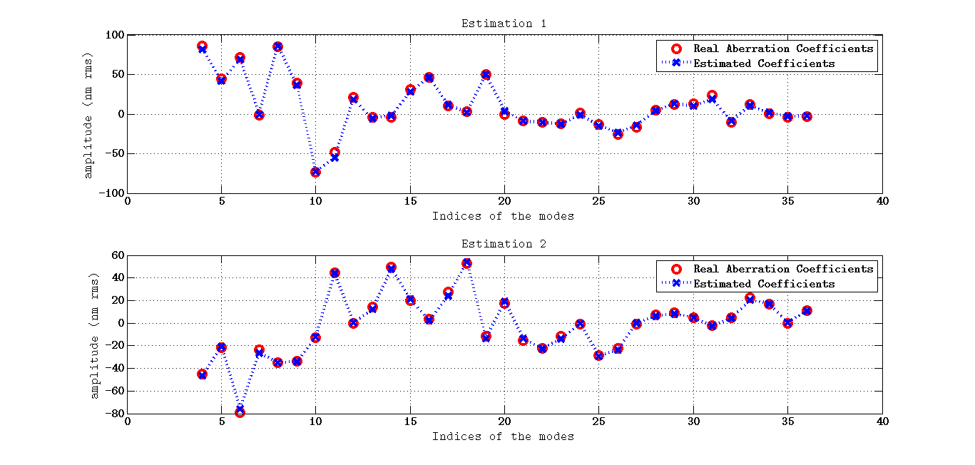
Figure 4 shows two examples of Phase Diversity estimation on $33$ Zernike coefficients with synthetic aberrations. The mean performance over $150$ simulations of Phase Diversity is given in Table 1.

infinity norm	rms	$2$ -norm
$5.1$	$2.0$	$11.7$

Table 1: Mean performance of Phase Diversity over 150 simulations. A simulation includes a new aberration vector, a new Gaussian noise pattern for the image and a new estimation. The performance is expressed as the Infinity Norm of the error which is the maximum absolute value, the Root-Mean-Square and finally the

2

-Norm which is the square root of the sum of the squares.

8.2 Image Reconstruction

Once the coefficients are estimated it is possible to reconstruct simulated images like in Figure 5.

8.3 Object Reconstruction

Phase Diversity estimates the object as well. Figure 6 shows the estimation of a point source in simulation.

9 Adaptive Optics Facility

The team for the tests included Johann Kolb and the author himself.

Results presented here are only two of the many tests performed on the ASSIST test bench for the AOF. The complete set of result is available in the technical report ruffioAOFPDtest [ruffioAOFPDtest]. An entire week was booked for these tests. In total $16$ iterations tests were performed as well as code validation tests like the linearity check briefly mentioned below. Another important experiment was the definition of spiders^†^†margin: The spiders are the structural elements fixing the secondary mirror from the edges of the primary mirror. ^†^†margin: The spiders are the structural elements fixing the secondary mirror from the edges of the primary mirror. but it has been skipped for this document.

9.1 Linearity Test

The linearity test is one of the first test that the author performed on the AOF. It is a good way to verify the behaviour of the algorithm. To do so we applied different amplitudes to the $14^{th}$ Zernike mode^†^†margin: The defocus is the $4^{th}$ ^†^†margin: The defocus is the $4^{th}$ on the AOF, recorded images and applied Phase Diversity. Eight different amplitudes have been tested from $0$ to $350\text{nm rms}$ with a step of $50\text{nm rms}$ . This mode was selected because it is usually well detected by the algorithm with low residuals on the other modes. For every coefficient we apply a positive and a negative offset for reconstructing the sole contribution of the mode by difference and the sole aberration by addition. The short result of the test is shown in Figure 7 and the complete results can be found in ruffioAOFPDtest [ruffioAOFPDtest].

One can see that the linearity is very good until a saturation of the amplitude of the estimated coefficient at $200\text{nm rms}$ even if it begins to deviate at $150\text{nm rms}$ . Besides the other modes are perturbed when the saturation is reached because the algorithm try to use other modes to reconstruct the aberration. ^†^†margin: It is very likely to be the $2\pi$ phase aberration limit indicated by ONERA. ^†^†margin: It is very likely to be the $2\pi$ phase aberration limit indicated by ONERA.

9.2 Iterations

Figure 8 shows the Point Spread Function of the AOF after and before Phase Diversity correction. Visually the image becomes clearly more symmetrical and portions of rings appears. The analysis of the two iterations is presented in Figure 9. The Projection Matrix used is available in Appendix 12.A Figure 21. One can see that the Strehl Ratio jump of $17\%$ at the first iteration and then go down a little. However the estimated aberrations are always converging toward zero. One should remember that it is only one of the $16$ iterations test performed on the AOF.^†^†margin: For the complete set of results see ruffioAOFPDtest [ruffioAOFPDtest]. ^†^†margin: For the complete set of results see ruffioAOFPDtest [ruffioAOFPDtest]. $17\%$ is the biggest jump that the author could reach in one iteration. Otherwise the highest Strehl reached was close to $80\%$ . However the Strehl is still quite unstable and the improvement is globally chaotic when iterating^†^†margin: Chaotic means that the Strehl Ratio went up and down. ^†^†margin: Chaotic means that the Strehl Ratio went up and down. . See the discussion in Chapter 4 for more comments.

^†^†margin: 4 Discussion

During the first half of 2014 the AOF was in Maintenance and Commissioning mode with GRAAL in ESO’s laboratory in Garching. There is therefore no immediate scientific goal to the current experiments on ASSIST.^†^†margin: Even if some performance requirements are tested. ^†^†margin: Even if some performance requirements are tested. The main purpose is to better understand the system in order to be able to identify possible problems. One of the problems AOF’s people faced was a very poor quality Point Spread Function. The usual method to improve the Strehl Ratio is to apply Phase Diversity. However it assumes that the problem comes from phase error in the non-common optical path. But the existing algorithm didn’t succeed. Different explanations were suggested but the main one was the existence of spiders in the pupil while the algorithm didn’t take account for them. The new author’s code actually proved using simulations and experimental tests^†^†margin: These tests are shown in ruffioAOFPDtest [ruffioAOFPDtest]. ^†^†margin: These tests are shown in ruffioAOFPDtest [ruffioAOFPDtest]. that it had not a noticeable impact on the result. Other paths to improve the estimation were explored but without success^†^†margin: For example a better sampled pupil has been tried or different hyper-parameters. ^†^†margin: For example a better sampled pupil has been tried or different hyper-parameters. . The author’s algorithm has proven itself reliable as it passed the linear test and it visually succeeds in removing the very low order aberrations. However the new code didn’t give better Strehl Ratio^†^†margin: The Strehl was stuck below $80\%$ ^†^†margin: The Strehl was stuck below $80\%$ and it is still very unstable so it convinced the team that the problem is not caused by low order phase aberrations that can be solved with the Deformable Mirror. The Strehl Ratio is also something complex to estimate and the existing algorithm are not very stable and robust. One could therefore partially question these values. Other explanation could include amplitude errors but they have not been estimated yet.^†^†margin: The pupil amplitude variations should indeed turn around $20-25\%$ . ^†^†margin: The pupil amplitude variations should indeed turn around $20-25\%$ . The existence of a half ring in the left image of Figure 8b strongly points toward this explanation. Indeed a Deformable Mirror can correct amplitude aberrations in only one half of the Point Spread Function.

References

Aller-Carpentier [2011] Emmanuel Aller-Carpentier. Extreme Adaptive Optics system optimization for High Contrast Imaging with the high Order Test bench. PhD thesis, Universidad Autonoma de Madrid, 2011.
Batalha et al. [2013] Nathalie M. Batalha et al. Planetary candidates observed by kepler. iii. analysis of the first 16 months of data. The Astrophysical Journal. Supplement Series., 2013.
Beuzit et al. [2008] J.-L. Beuzit, M. Feldt, K. Dohlen, D. Mouillet, P. Puget, F. Wildi, L. Abe, J. Antichi, A. Baruffolo, P. Baudoz, A. Boccaletti, M. Carbillet, J. Charton, R. Claudi, M. Downing, C. Fabron, P. Feautrier, E. Fedrigo, T. Fusco, J.-L. Gach, R. Gratton, T. Henning, N. Hubin, F. Joos, M. Kasper, M. Langlois, R. Lenzen, C. Moutou, A. Pavlov, C. Petit, J. Pragt, P. Rabou, F. Rigal, R. Roelfsema, G. Rousset, M. Saisse, H.-M. Schmid, E. Stadler, C. Thalmann, M. Turatto, S. Udry, F. Vakili, and R. Waters. Sphere: a ’planet finder’ instrument for the vlt. In Society of Photo-Optical Instrumentation Engineers (SPIE) Conference Series, volume 7014 of Society of Photo-Optical Instrumentation Engineers (SPIE) Conference Series, July 2008. 10.1117/12.790120. URL http://adsabs.harvard.edu/abs/2008SPIE.7014E..18B.
Bordé and Traub [2006] Pascal J. Bordé and Wesley A. Traub. High-contrast imaging from space: Speckle nulling in a low aberration regime. Astrophysical Journal, 2006.
Born and Wolf [1980] Max Born and Emil Wolf. Principle of Optics. Cambridge University Press, 6 edition, 1980.
Cavarroc et al. [2005] C. Cavarroc, A. Boccaletti, P. Baudoz, T. Fusco, and D. Rouan. Fundamental limitations on earth-like planet detection with extremely large telescopes. Astronomy & Astrophysics, September 2005.
Codona [2013] J. L. Codona. Differential optical transfer function wavefront sensing. Optical Engineering, 2013.
Codona et al. [2008] Johanan L. Codona, Matthew A. Kenworthy, and Michael Lloyd-Hart. A novel wfs technique for high-contrast imaging: Phase sorting interferometry (psi). SPIE, 2008.
Loose [2011] Christina Loose. Speckle characterisation and supression for high-contrast imaging on an extreme adaptive optics testbench. Master’s thesis, Technische Universität München, 2011.
Macintosh et al. [2006] B. Macintosh, J. Graham, D. Palmer, R. Doyon, D. Gavel, J. Larkin, B. Oppenheimer, L. Saddlemyer, J. K. Wallace, B. Bauman, J. Evans, D. Erikson, K. Morzinski, D. Phillion, L. Poyneer, A. Sivaramakrishnan, R. Soummer, S. Thibault, and J.-P. Veran. The gemini planet imager. In Society of Photo-Optical Instrumentation Engineers (SPIE) Conference Series, volume 6272 of Society of Photo-Optical Instrumentation Engineers (SPIE) Conference Series, june 2006. 10.1117/12.672430. URL http://adsabs.harvard.edu/abs/2006SPIE.6272E..0LM.
Mahajan [1982] Virendra N. Mahajan. Strehl ratio for primary aberrations: some analytical results for circular and annular pupils. Journal of the Optical Society of America, 72(9), September 1982.
Mahajan [1983] Virendra N. Mahajan. Strehl ratio for primary aberrations in terms of their aberration variance. Journal of the Optical Society of America, 73(6), June 1983.
Marois et al. [2006] Christian Marois, David Lafrenière, René Doyon, and Bruce Daniel Macintosh, Macintosh. Angular differential imaging: A powerful high-constrast imaging technique. The Astrophysical Journal, April 2006.
Martinache [2011] Frantz Martinache. Kernel-phases for high-contrast detection beyond the reolsution limit. SPIE, 2011.
Paul et al. [2013] B. Paul, L. M. Mugnier, H.-F. Sauvage, and K. Dohlen. High-order myopic coronagraphic phase diversity (coffee) for wave-front control in high-contrast imaging ssystem. Optical Society of America, 2013.
Soummer et al. [2009] R. Soummer, L. Pueyo, A. Ferrari, C. Aime, A. Sivaramakrishnan, and N. Yaitskova. Apodized pupil lyot coronagraphs for arbitrary apertures. ii. theoretical properties and application to extremely large telescopes. The Astrophysical Journal, April 2009.
Soummer [2004] Rémi Soummer. Apodized pupil lyot coronagraphs for arbitrary telescope apertures. The Astrophysical Journal, December 2004.
Wildi et al. [2011] Francois Wildi, Francesco Pepe, Bruno Chazelas, Gaspare Lo Curto, and Christophe Lovis. The performance of the new fabry-perot calibration system of the radial velocity spectrograph harps. In Techniques and Instrumentation for Detection of Exoplanets, 2011.

Part II Electric Field Conjugation

^†^†margin: 5 Theory

This chapter develops the theory behind Electric Field Conjugation. The essential of this part is inspired from giveon2011 [giveon2011]. The core method is something that has been used extensively in laboratory however it is not yet very common on-sky.

Electric Field Conjugation is a method to darken a predefined area in a coronagraphic image using a Deformable Mirror and the science camera. The nice side of this method is its simplicity. Indeed there is no estimation theory involved here and it is conceived so that everything is linear. The only real mathematical tool used is the Singular Value Decomposition but basic knowledge on Pseudo-Inverse is sufficient. The idea of Electric Field Conjugation is to record images while applying so called probes positively and negatively on the Deformable Mirror. The probes are shapes of the Deformable Mirror which result in adding a known complex amplitude to the speckles in the focal plane. Based on some assumptions the subtraction of the two images is linearly proportional to the electric field in the focal plane. Besides using Fourier Optics the electric field itself is linearly related to the phase in the pupil at least to the first order and therefore to the shape of the Deformable Mirror. Altogether it means that the relation between the shape of the Deformable Mirror and its effect on the intensity in the detector is linear. It means that one is able to define a shape of the Deformable Mirror for cancelling out the speckles. This shape is in practice expanded on a base of modes. For example the effect of Fourier modes is to enlighten a spot at a position defined by the frequency of the sine in the pupil.

Author’s Contributions

One contribution has been to make the mathematical demonstration cleaner. The Taylor expansions were indeed not rigorously made which requires some not well justified approximations. The author solved the problem in the case of coronagraphic images. The author also suggested to use singular modes instead of Fourier modes which should be in theory more efficient. ^†^†margin: The definition of a probe and a mode will be detailed in Section 14. ^†^†margin: The definition of a probe and a mode will be detailed in Section 14.

The section begins first with a short bibliography of Electric Field Conjugation. Then it develops the intensity expression in the focal plane.^†^†margin: Because of number of pages requirement most of the interesting demonstrations are in Appendix. ^†^†margin: Because of number of pages requirement most of the interesting demonstrations are in Appendix. Using this model it explains how the electric field can be estimated in the focal plane using intensity measurements. Then it develops how the speckle correction can be performed using probes and modes themselves described in the following section. To finish a more practical description of Electric Field Conjugation is given for whoever wants to apply it in real life.

10 State of the Art

Many different types of correction algorithm have been developed based on the estimation of the complex electric field in the focal plane.^†^†margin: The author didn’t read all the papers so he will only cite the ones he knows. ^†^†margin: The author didn’t read all the papers so he will only cite the ones he knows. During his master thesis at the European Southern Observatory (ESO) the author based his work on the formulation of the problem by giveon2011 in [giveon2011] and [giveon2007]. Others similar methods have been tried elsewhere for example martinacheSUBARUEFC [martinacheSUBARUEFC] with a Speckle Nulling technique on-sky at the Subaru telescope. However the algorithm presented in this document seems more straightforward. thomas2010 in [thomas2010] shows results of Electric Field Conjugation at the Laboratory of Adaptive Optics in Santa Cruz. She reached an additional order of magnitude in a $5\times 5(\lambda/d)$ rectangle area at a distance of $6.5(\lambda/d)$ . However thomas2010 kept separated the estimation of the electric field and the correction in her algorithm. Besides she based the estimation on a simulation of the bench which requires a very good knowledge of it. The method developed by the author and Markus Kasper is simpler to implement because all the calibrations are measured and there is no estimation of the electric field.

A previous master student jankowsky2012 worked on Electric Field Conjugation in 2012 at the ESO for his master thesis [jankowsky2012]. He tried to apply Electric Field Conjugation on the High Order Testbench (HOT)^†^†margin: The High Order Testbench purpose was to test Extreme Adaptive Optics systems. ^†^†margin: The High Order Testbench purpose was to test Extreme Adaptive Optics systems. from ESO in the same way it was applied on a bench at the Institut de Planétologie et d’Astrophysique de Grenoble (IPAG) called Fresnel-FRee Experiment for EPICS⁹⁹ 9 EPICS means Exoplanet Imaging Camera and Spectrograph (FFREE). However the speckles on FFREE were artificially added using a phase screen before trying to suppress them. This experience reached a maximum contrast improvement of $40$ in term of the Root-Mean-Square of the speckles in a rectangle area. The results can be found in verinaudFREEEFC [verinaudFREEEFC].

11 Model

The complex amplitude in the pupil plane is defined by,

\mathcal{P}(x,y)=\mathcal{P}_{m}(x,y)e^{i(\phi(x,y)+\psi(x,y)+\omega(x,y))},

(7)

With $P_{m}(x,y)$ the pupil mask.^†^†margin: Note that the model doesn’t include amplitude aberrations. ^†^†margin: Note that the model doesn’t include amplitude aberrations. $x$ and $y$ are the spatial coordinates in the pupil normalized by the pupil mask diameter. $\phi(x,y)$ , $\psi(x,y)$ and $\omega(x,y)$ are the phase respectively of the aberrations, the probes and the correction phase. The correction phase is later expanded on modes.

Electric Field Conjugation is dealing with coronagraphic images so that the complex amplitude in the focal plane can’t be computed using simply one Fourier Transform. However it would use a series of Fourier Transforms to take into account the succession of pupil and focal planes in which are the apodizer, the focal-mask and the Lyot-stop.^†^†margin: For more about the Apodized-Lyot-Coronagraph see Section 9.D.2. ^†^†margin: For more about the Apodized-Lyot-Coronagraph see Section 9.D.2. This transformation is a combination of linear operators so that it is also linear and it is noted $\mathcal{C}$ standing for Coronagraph. Therefore the complex amplitude in the focal plane is given by,

\mathcal{D}(\xi,\eta)=\mathcal{C}\left(\mathcal{P}\right)=\mathcal{C}\left(\mathcal{P}_{m}e^{i(\phi+\psi+\omega)}\right),

(8)

With $D(\xi,\eta)$ the complex amplitude in the focal plane. $\xi$ and $\eta$ are the spatial coordinates in the focal plane normalized by $\lambda/d$ ^†^†margin: The unit of $\xi$ and $\eta$ is sometimes called resel. ^†^†margin: The unit of $\xi$ and $\eta$ is sometimes called resel. .

The phase $\omega$ is ignored for now and $\phi$ and $\psi$ are assumed small compared to unity. In order to make the notation more compact the operator $\mathcal{C}$ will now be noted with an upper bar. ^†^†margin: The upper bar is sometimes used for conjugation but here the conjugate of $z$ is noted $z^{\ast}$ . ^†^†margin: The upper bar is sometimes used for conjugation but here the conjugate of $z$ is noted $z^{\ast}$ . Expanding the expression of the intensity $\mathcal{I}=\mathcal{D}\mathcal{D}^{\ast}$ with a second Taylor expansion gives,

$\displaystyle\mathcal{I}$	$\displaystyle=\left\lvert\overline{\mathcal{P}_{m}}\right\rvert^{2}$	$\displaystyle 0\,\text{Order,}$
	$\displaystyle+2\text{Re}\left[i\left(\overline{\mathcal{P}_{m}}\right)^{\ast}\left(\overline{\mathcal{P}_{m}\phi}+\overline{\mathcal{P}_{m}\psi}\right)\right]$	$\displaystyle 1^{st}\,\text{Order,}$
	$\displaystyle-2\text{Re}\left[\overline{\mathcal{P}_{m}}\left(\overline{\mathcal{P}_{m}\frac{\phi^{2}}{2}}+\overline{\mathcal{P}_{m}\frac{\psi^{2}}{2}}+\overline{\mathcal{P}_{m}\psi\phi}\right)^{\ast}\right]$	$\displaystyle 2^{nd}\,\text{Order,}$
	$\displaystyle+\left\lvert\overline{\mathcal{P}_{m}\phi}\right\rvert^{2}+\left\lvert\overline{\mathcal{P}_{m}\psi}\right\rvert^{2}+2\text{Re}\left[\left(\overline{\mathcal{P}_{m}\phi}\right)^{\ast}\overline{\mathcal{P}_{m}\psi}\right]$	$\displaystyle\dots$	(9)

The complete demonstration is given in Appendix Appendix 13.A.

12 Electric Field Estimation

The principle of Electric Field Conjugation is to apply the probe $\psi$ positively and negatively. As it is demonstrated in Appendix 13.B and assuming a perfect coronagraph the difference between the two resulting images is linearly proportional to the electric field of the speckles. The only terms remaining of the difference in (9) are indeed the one proportional to $\psi$ . Using vector and matrix representation of the variables the problem takes the form,^†^†margin: The function in the pupil or in the focal plane are discretized and shaped in vector form. ^†^†margin: The function in the pupil or in the focal plane are discretized and shaped in vector form.

\underbrace{\left[\begin{array}[]{c}\frac{1}{2}(I_{1}^{+}-I_{1}^{-})\\ \frac{1}{2}(I_{2}^{+}-I_{2}^{-})\end{array}\right]}_{\delta I_{\Phi}}=2\underbrace{\left[\begin{array}[]{cc}\text{Re}\left[C\Psi_{1}\right]&\text{Im}\left[C\Psi_{1}\right]\\ \text{Re}\left[C\Psi_{2}\right]&\text{Im}\left[C\Psi_{2}\right]\\ \end{array}\right]}_{E}\left[\begin{array}[]{c}\text{Re}\left[C\Phi\right]\\ \text{Im}\left[C\Phi\right]\end{array}\right],

(10)

With $\Psi_{1}$ and $\Psi_{2}$ two different probe vectors and $I_{1}$ respectively $I_{2}$ the vector of the pixel intensities for the respective probes. $I_{k}^{+}$ and $I_{k}^{-}$ correspond to the use of the positive and the negative offset of the probe.
(10) is the core of Electric Field conjugation

13 Correction

The goal of Electric Field Conjugation is to cancel the term $\phi$ using the correction phase $\omega$ in,

\mathcal{P}=\mathcal{P}_{m}e^{i(\phi+\omega)},

(11)

so that the speckles disappear. $\omega$ is created using the Deformable Mirror so that it can be defined as a vector of commands $A$ for the actuators. The demonstration in Appendix 13.C shows that $A$ can be obtained from,

GA=-\delta I_{\Phi}\quad\text{or}\quad A=-R\delta I_{\Phi},

(12)

With $G$ a so called Interaction Matrix and $R$ its inverse called the Reconstruction Matrix. ^†^†margin: The expression of $G$ is given in Appendix 13.C. ^†^†margin: The expression of $G$ is given in Appendix 13.C. The Interaction Matrix $G$ should be either computed through simulations or directly measured. ^†^†margin: It is quite common to simulate the Interaction Matrix however measurements prevent one from hidden parameters, biases or more generally wild assumptions. ^†^†margin: It is quite common to simulate the Interaction Matrix however measurements prevent one from hidden parameters, biases or more generally wild assumptions.

14 Dark Hole Definition

14.1 Modes

The modes are a base of functions on which the correction phase $\omega(x,y)$ is expanded. The base should be complete enough so that every pixel of the area can be corrected. The number of independent modes is limited by the number of actuators. ^†^†margin: In the experiences done by the author on SPHERE it seems like there is no further improvement when using more than $\simeq 150$ modes. ^†^†margin: In the experiences done by the author on SPHERE it seems like there is no further improvement when using more than $\simeq 150$ modes.

The problem as defined in (12) was presented with $A=[a_{1}\,a_{2}\,\dots\,a_{K}]^{\mathsf{T}}$ being the actuators commands however it is actually more generally the coordinate vector of the phase $\Omega$ in the base of the modes.

\Omega=\sum_{k=1}^{K}a_{k}Z_{k}=ZA,

(13)

With $Z_{k}$ the modes as vectors containing the pupil phase values and $Z$ the matrix formed with the column vectors $Z_{k}$ . The method to obtain the commands vector from the modes for the actuators is given in Section 13.D.1.

The contribution of a mode to the electric field in the focal plane is to the first order equal to the Fourier Transform of the phase times the pupil mask.^†^†margin: It comes from a first order Taylor expansion and the linearity of $\mathcal{C}$ in Equation 8. ^†^†margin: It comes from a first order Taylor expansion and the linearity of $\mathcal{C}$ in Equation 8. So one can roughly infer the effect of a mode directly from the phase instead of from the complex amplitude.

It is then straightforward to define sine and cosine functions which are called Fourier modes. Their Fourier Transform being a pair of Dirac functions the effect on the detector will be two symmetric non coronagraphic Point Spread Function^†^†margin: If they are not on axis the coronagraph is negligible. ^†^†margin: If they are not on axis the coronagraph is negligible. centred on a pixel defined by the frequency of the wave. A detailed description of the Fourier modes with closed form expression and example figure is given in Section 13.D.2 and Figure 22.

More efficient modes can be defined from the Singular Value Decomposition of the Interaction Matrix. The author called them Singular Modes. The detailed explanation is given in Section 13.D.3.

14.2 Probes Definition

The probes noted $\psi$ in the previous sections are phase function produced by the Deformable Mirror for introducing diversity into the measurement and then retrieving the electric field from intensities. Their effect in the focal plane should cover all the area of interest^†^†margin: Even if it is also possible to patch probes. ^†^†margin: Even if it is also possible to patch probes. . Two probes should have different phase for any point in the focal plane falling in the area. The best probes would have orthogonal vectors which means a difference in phase of $\frac{\pi}{2}$ in the focal plane. giveon2011 [giveon2011] gives an example of probes for making a rectangle in the detector. Their closed form expression, their explanation and a figure is available in appendix Appendix 13.E and Figure 23. ^†^†margin: New formula for rotated probes is also available. ^†^†margin: New formula for rotated probes is also available.

14.3 Area

The area of interest also called dark hole can have any shape. However Electric Field Conjugation cannot correct for both phase and amplitude aberrations if the area overlap with itself when mirrored. It means for instance that as long as the area remains in one half of the image the algorithm is able to correct amplitude aberration as well. This is due to the fact that the Deformable Mirror can only act on the phase. ^†^†margin: However the author doesn’t know yet a proper explanation for this… ^†^†margin: However the author doesn’t know yet a proper explanation for this…

Besides the spatial frequency in the pupil is limited by the distance between two actuators. The limitation in spatial frequency in the pupil plane results in the impossibility of correcting speckles too far from the center. For example if the Deformable Mirror has an array of $40\times 40$ actuators it can produce a maximum of $40/2=20$ periods on its surface and therefore the limit of correction would be at $20(\lambda/d)$ . Even inside the boundaries the efficiency of the correction is not constant with the distance to the center. Some frequencies are indeed not well reproduced by the discrete array of actuators. In practice one can neither correct too close of the center because of the residual leaking light of the coronagraph. Because of all these constraints the area should not be too far, neither too close and not too big…

15 Application

15.1 Measurements

The measurements for Electric Field Conjugation consist in doing the following for each probe,

1.

Apply probe positively and negatively to the Deformable Mirror and take an image for both.
2.

Extract the pixels of the area of interest from both images.
3.

Reshape the pixels in vector form.
4.

Subtract the vector of the positive probe to the vector of the negative probe and divide by two.

Then one needs to concatenate the resulting vectors of each probe for building the measurement vector called $\delta I_{\Phi}$ in (12).
It is important that the centroid of the Point Spread Function doesn’t move during the measurements and it has to be at the same relative sub-pixel position than when building the Interaction Matrix $G$ .
In practice a dark exposure was also taken before and after the acquisition of the image. Besides each image where taken twice in order to estimate the photon noise in the correction vector. ^†^†margin: A reference image with no applied probe can also be taken for measuring the intensity in the dark area. ^†^†margin: A reference image with no applied probe can also be taken for measuring the intensity in the dark area. For SPHERE a template was implemented on the instrument to run this sequence of image acquisition. The template instructions are given in kasperNCPATemplate2014 [kasperNCPATemplate2014].

15.2 Interaction Matrix

The Interaction Matrix can be either simulated or directly measured. An example of synthetic matrix is given in Figure 10.^†^†margin: It is easier and more secure to measure it. However this calibration takes a long time when performed on a real system. For example building a Interaction Matrix for SPHERE with two probes and a hundred modes takes roughly two hours. ^†^†margin: It is easier and more secure to measure it. However this calibration takes a long time when performed on a real system. For example building a Interaction Matrix for SPHERE with two probes and a hundred modes takes roughly two hours. Beforehand one needs to notice that the columns of $G$ are measurement vectors when a single mode is applied $\delta I_{\Omega}$ . Therefore building the Interaction Matrix consists in applying each mode one by one and then construct the measurement vector as explained in Section 15.1. This naive approach would work only if there were no existing aberration while doing it. The solution to get rid of the aberrations is to apply the modes positively and negatively and then subtracting the two resulting measurement vectors. The demonstration is given in appendix Appendix 13.F.

To conclude the steps for building the Interaction Matrix consists in doing for each mode and for each probe,

1.

Take an image for all possible combinations of positive and negative probes and positive and negative modes.
2.

Extract the pixels of the area of interest from all images.
3.

Reshape the pixels in vector form.
4.

Subtract the vectors of the positive probe to the vectors of the negative probe for each mode and divide by two.
5.

Subtract the difference vectors from last step of the positive and the negative mode.

Then one needs to concatenate the vectors of the different probes for building the measurement vector. To finish the resulting vectors should be concatenated together as column vectors for building the Interaction Matrix.

15.3 Iterations

Once the measurement vector $\delta I_{\Phi}$ is build one just needs to multiply it with the Reconstruction Matrix,

A=-R\delta I_{\Phi}=-G^{\dagger}\delta I_{\Phi}.

(14)

^†^†margin: Note that even if a Pseudo-Inverse is used here the author uses in practice a filtered Singular Value Decomposition. ^†^†margin: Note that even if a Pseudo-Inverse is used here the author uses in practice a filtered Singular Value Decomposition.

Again $A$ is the coordinate vector of the correction phase in the modal base. The command vector $\alpha$ for the Deformable Mirror can then be computed from $A$ using the influence functions using,

\alpha=I_{f}^{\dagger}ZA,

(15)

With $I_{f}$ the influence function matrix and $Z$ the matrix to transform modal base coordinates into pupil phase. The computation of the commands can also be done by adding the commands of each mode with the correct amplitude of $A$ .

Once the correction commands are applied another iteration can be performed. Electric Field Conjugation assumes the linearity of the system so it needs a few steps to reach the best correction. ^†^†margin: For an example of simulated EFC iterations see Section 16. ^†^†margin: For an example of simulated EFC iterations see Section 16.

In order to measure the performance of the iterations one can measure the standard deviation of the intensity inside the area of interest. The ratio between the standard deviation of the last step and the first image corresponds to the contrast improvement.

^†^†margin: 6 Results

This chapter exposes the simulated or experimental results of Electric Field Conjugation applied on SPHERE.

Author’s Contributions

This whole section is author’s contribution. The simulation were done using Matlab. The author developed a set of functions for computing Fourier optics optionally including perturbations or coronagraphs for instance. An overview of the code is available in EFCPDCodes [EFCPDCodes]. When experimenting on SPHERE the author did also all the data reduction and the computation of the correction vectors with tools he implemented.

16 Simulations

For the author the first goal of the simulations were to check his understanding of the method. The simulation are indeed not required for applying Electric Field Conjugation on a real system^†^†margin: This is true only if one measures the Interaction Matrix instead of using a synthetic one. ^†^†margin: This is true only if one measures the Interaction Matrix instead of using a synthetic one. . However a few tools of the simulations were still used on the real system. For example the definition of the probes and the modes commands for feeding the Deformable Mirror are the same. Besides the image reduction is identical in simulation and on the instrument.

Then the simulations were used to give an idea of what could be expected and how to reach the best performance. This aspect has a limited range because the model is too perfect compared to the real system.

Note

Because of the number of pages requirement almost all the simulations can be found in Appendix 14.A. ^†^†margin: In Appendix 14.A one can also find the improvement with singular modes, the effect of the distance of the area and the combined effect of the number of modes and the number of pixels of the area. ^†^†margin: In Appendix 14.A one can also find the improvement with singular modes, the effect of the distance of the area and the combined effect of the number of modes and the number of pixels of the area.

16.1 Simulation Principles

The principle of the simulation is to do the following actions, ^†^†margin: Note that an how-to tutorial is available in [EFCPDCodes]. ^†^†margin: Note that an how-to tutorial is available in [EFCPDCodes].

1.

Define the optics,
2.

Load the influence functions of the Deformable Mirror,
3.

Construct the probes and the modes,
4.

Construct the Interaction Matrix by simulating images with the probes and the modes,
5.

Invert the Interaction Matrix,
6.

Apply a few iterations of Electric Field Conjugation,
7.

And analyze the results.

16.2 General Parameters

The coronagraph of SPHERE is an Apodized-Lyot-Coronagraph which is simply modeled by its different planes: apodization function, focal plane mask and Lyot-Stop ^†^†margin: For more about the Apodized-Lyot-Coronagraph see Section 9.D.2. ^†^†margin: For more about the Apodized-Lyot-Coronagraph see Section 9.D.2. . The masks correspond to the configuration used on SPHERE and especially in Section 17.1.

If nothing is specified Fourier modes refer to modes centred on the unit grid. It means they are spaced by $1(\lambda/d)$ ¹⁰¹⁰ 10 This is roughly $3$ pixels for IRDIS SPHERE. in both axes in the detector. Singular modes are here defined from the Singular Value Decomposition of an Interaction Matrix built with a pixel based set of modes.^†^†margin: When simulating with singular modes a new Interaction Matrix with only the singular modes is built. However the result by just filtering the pixel defined Interaction Matrix to keep the same number of singular modes is almost equivalent in simulation. ^†^†margin: When simulating with singular modes a new Interaction Matrix with only the singular modes is built. However the result by just filtering the pixel defined Interaction Matrix to keep the same number of singular modes is almost equivalent in simulation. The modes respectively the probes have an amplitude of $0.01\text{rad}$ respectively $0.1\text{rad}$ . The probe needs higher amplitude because it is spread on a bigger area. To finish the noise in the phase for creating the speckles has a standard deviation of $0.01\text{rad}$ .

16.3 Simulated Iterations

The first test is to verify that running Section 16.1 indeed creates a dark hole in the speckles of the image.

For a simple rectangle case the result of two iterations is given in Figure 11 and the mean performance values over ten simulations is given in Table 2.

modes	rms	intensity
$132$ Fourier	$140$	$183$

Table 2: Contrast improvement for the study case of Figure 11 with a

5\times 10(\lambda/d)

rectangle

10(\lambda/d)

away from the center. The gain is computed in term of the Root-Mean-Square value and the total intensity in the dark hole area. The values are the result of the mean over ten simulations.

17 SPHERE

The team for the tests included Markus Kasper, Christophe Vérinaud and the author himself.

17.1 General Parameters

The experiments on SPHERE were done using an Apodized-Lyot-Coronograph ^†^†margin: The APO1 apodizer, the ALC2 mask (4 $\lambda/d$ in diameter) and ST_ALC Lyot-Stop were used. See the technical documentation [SPHEREcoro2012]. ^†^†margin: The APO1 apodizer, the ALC2 mask (4 $\lambda/d$ in diameter) and ST_ALC Lyot-Stop were used. See the technical documentation [SPHEREcoro2012]. configuration and the internal fibre as a infrared light source. A narrow-band filter in H-band at $1.6\mu m$ was used.

The first attempts were realized with the Adaptive Optics in open-loop. The tip-tilt correction was however in closed-loop so that the image doesn’t move too much on the detector. Open-loop is indeed slightly easier to manage because applying a shape to the Deformable Mirror corresponds simply to the addition of a voltage vector to the commands. When doing so in closed-loop the feedback would automatically kill the shape for going back to a flat wavefront. However the assumption of negligible internal convection in SPHERE^†^†margin: SPHERE is closed and cooled environment. ^†^†margin: SPHERE is closed and cooled environment. was too optimistic so that the experiment had to be done in closed-loop. In that case the reference slopes of the wavefront sensor need to be used for applying shapes to the Deformable Mirror instead of the voltages. When doing so a problem of synchronization between the image acquisition and the Deformable Mirror occurred. Indeed loading reference slopes needs time but the delay is random.^†^†margin: The delay is up to two seconds. ^†^†margin: The delay is up to two seconds. Therefore when acquiring images the right shape of the mirror was sometimes applied at the middle of the integration time. The solution found was to pause the system for two seconds between the sending of the reference slopes and the image acquisition. ^†^†margin: This is not optimized and lot of time is wasted because of that. However the system does not have a proper synchronization with a flag telling when it is ready to go. So there is no choice until it is implemented. ^†^†margin: This is not optimized and lot of time is wasted because of that. However the system does not have a proper synchronization with a flag telling when it is ready to go. So there is no choice until it is implemented. Including overheads one image requires in total about ten seconds. An example of a mode and an example of a probe are given in Appendix in Figure 27.

All the image acquisition part was done using on-board SPHERE software but all the data reduction and the computation of the commands or slopes vectors were done using external Matlab codes.

The amplitudes of the probes and of the modes were adjusted by hand. The used amplitudes were not always recorded so that the author can’t give their value. Still it can be noticed that the amplitude of the probes was decreased^†^†margin: However this was not proven to have an effect… ^†^†margin: However this was not proven to have an effect… at each iteration to follow the intensity drop in the dark hole. The criteria for a fine amplitude were that one could visually see the effect of a probe or a mode but without being brighter than the speckles.

Warning

A mistake was made in the scripts when iterating with simulated interaction matrices so that the author can’t be exactly sure that the right matrices were used. This is particularly relevant for the first rectangle case where the simulated Interaction Matrix works surprisingly well. It could be that in fact it was the measured matrix which was used. In order to validate this result one should try it again.

17.2 Rectangle

The first successful attempt of Electric Field Conjugation iterations was performed on a $5\times 10(\lambda/d)$ rectangle at a distance of $10(\lambda/d)$ of the center. Fourier modes and singular modes were tested as well as a synthetic Interaction Matrix. The resulting corrected area for the best case with $132$ Fourier modes is shown in Figure 12. The performance for all the tests is given in Table 3. One can find the complete results in Appendix in Figure 28, Figure 29 and Figure 30.

17.3 Arc

The second experiment was done on a quarter of a ring with a width of $5(\lambda/d)$ and a mean radius of $10(\lambda/d)$ . $125$ singular modes were used. Again a comparison between a synthetic and a measured Interaction Matrix was performed. However in this case the synthetic matrix didn’t performed well. The results are given in Table 4 and the resulting dark hole for the measured Interaction Matrix is shown in Figure 13. One can find the complete results in Appendix in Figure 31, Figure 32 and Figure 33.

17.4 Big Rectangle

The last test was done on a big area formed by a $8\times 16(\lambda/d)$ rectangle at a distance of $11(\lambda/d)$ of the center. A synthetic Interaction Matrix with 306 Fourier modes was used. The results are given in Table 5 and the images are shown in Figure 14. One can find the complete results in Appendix in Figure 34 and Figure 35.

modes	im	cond.	rms	rms (small)
$132$ Fourier	Measured	$87$	$10.1$	$13.3$
$109$ Singular	Measured	$33$	$9.1$	$12.5$
$109$ Singular	Synthetic	$36$	$7.1$	$7.8$

Table 3: Maximum contrast gain when iterating on a

5\times 10(\lambda/d)

rectangle at a distance of

10(\lambda/d)

of the center with different sets of modes. The columns are respectively indicating from left to right the set of modes, the type of Interaction Matrix, its conditioning number, the Root-Mean-Square contrast improvement in the area respectively in a smaller area without the edges.

modes	im	cond.	rms	rms (small)
$125$ Singular	Measured	$10$	$6.1$	$7.2$
$125$ Singular	Synthetic	$5$	$1.3$	$1.3$

Table 4: Maximum contrast gain when iterating on a quarter of a ring with a width of

5(\lambda/d)

and a mean radius of

10(\lambda/d)

using

125

singular modes. The columns are respectively indicating from left to right the set of modes, the type of Interaction Matrix, its conditioning number, the Root-Mean-Square contrast improvement in the area respectively in a smaller area without the edges.

modes	im	cond.	rms	rms (small)
$306$ Fourier	Synthetic	$36$	$2.0$	$2.3$

Table 5: Maximum contrast gain when iterating on a

8\times 16(\lambda/d)

rectangle at a distance of

11(\lambda/d)

of the center with

306

Fourier modes and a synthetic Interaction Matrix. The fourth respectively the last columns indicates the Root-Mean-Square contrast improvement in the area a smaller area without the edges.

^†^†margin: 7 Discussion and Perspective

The ultimate goal of high contrast imaging is the observation of an earth like planet in the habitable zone of its host star. In the case of $G2$ -type star like the Sun with an habitable zone around $1\text{AU}$ ^†^†margin: $1\text{AU}\approx 1.5\,10^{11}\text{m}$ ^†^†margin: $1\text{AU}\approx 1.5\,10^{11}\text{m}$ the required contrast is $2\,10^{-10}$ . Although it depends slightly on the albedo and the orbital position of the planet. This contrast is still clearly not achievable yet. The first step would probably be to look around an $M$ -type star because it requires a contrast of about only $10^{-8}$ . However the habitable zone is situated much closer to the star around $0.1\text{AU}$ and it becomes challenging to have a good contrast at this kind of separations. By definition of the parsec^†^†margin: $1\text{parsec}\approx 3.1\,10^{16}\text{m}$ ^†^†margin: $1\text{parsec}\approx 3.1\,10^{16}\text{m}$ the angular separation between a planet and its star separated by $1\text{AU}$ and $1\text{parsec}$ away from Earth is $0.1\text{arcsec}$ . This corresponds to $2.4(\lambda/d)$ ^†^†margin: It is about $8$ pixels on IRDIS SPHERE. ^†^†margin: It is about $8$ pixels on IRDIS SPHERE. for an instrument on the Very Large Telescope at a wavelength of $1.6\mu m$ . In the case of SPHERE it already falls in the Coronagraphic halo. Besides this value is inversely proportional to the distance of the stars. ^†^†margin: The closest star Proxima Centauri is at $1.3\text{parsec}$ . ^†^†margin: The closest star Proxima Centauri is at $1.3\text{parsec}$ . This is therefore a job for Extremely Large Telescopes with resolution of around $0.006$ to $0.007\text{arcsec}$ in $J$ band. They would hopefully be able to image the habitable zone of nearby stars between $1$ to $10\text{parsec}$ . SPHERE was never meant to observe Earth-like planets anyway but to observe giant extra-solar-planets at a distance of $1$ to $100\text{AU}$ of their star and in a range of $5$ to $15(\lambda/d)$ on the detector. A fine contrast is possible either with a relatively faint star or with a really bright young planet still emitting heat from its formation.

SPHERE has a raw coronagraphic speckle contrast of about $8\,10^{-6}$ . It might be possible to gain a factor $7$ with Spectral Differential Imaging marois2006 [marois2006] and another factor $10$ with Angular Differential Imaging. However this stays to be demonstrated during the next SPHERE commissionings^†^†margin: For now the integration time previously used was too short. ^†^†margin: For now the integration time previously used was too short. . So far with the previous commissionings a contrast of $5\,10^{-7}$ was demonstrated. The highest demonstrated gains with Spectral respectively Differential Imaging are $30$ respectively $10$ . These techniques brings the contrast of SPHERE up to $1.1\,10^{-7}$ .

Electric Field Conjugation has just proven to be able to divide another factor $10$ bringing the contrast to $10^{-8}$ . It is really getting closer to the ideal value. Although it is really a net gain only with very long exposure observations. Indeed the photon noise of the averaged speckles from the atmosphere would otherwise be dominant. The caveat of Electric Field Conjugation is that the position of the planet has to be known in advance for defining the dark hole. This method can therefore most efficiently be used for follow up studies once the planet has been discovered.^†^†margin: Or one could be very lucky… ^†^†margin: Or one could be very lucky… However Electric Field Conjugation has proven to be very efficient and it will very likely become a key element for improving the contrast on SPHERE.

Spectral or Angular Differential Imaging and Electric Field Conjugation are all three dealing with the same speckles. One could find surprising that the contrast improvement of each method can be multiplied when applied together. This is however validated by the experience. Even if it is not really intellectually convincing the reason is probably that each uses a different property of the speckles.

The size of the main mirror of the telescope is also important for improving the contrast. The gain corresponds to the square ratio of the size of the mirrors while keeping the quasi-static aberrations at a constant level. For example the gain of the Extremely Large Telescope in comparison with the Very Large Telescope is $\left(\frac{39\text{m}}{8\text{m}}\right)^{2}s=25$ .

The last option to gain contrast is to go in space but then the costs have no equivalent. It is interesting to remember that the price of the James Webb Telescope is estimate at about $\$9$ billions in 2013^†^†margin: When it was estimated at $\$0.5$ billions in 2007… ^†^†margin: When it was estimated at $\$0.5$ billions in 2007… . The price of an Extremely Large Telescope is only estimated to $\$1$ billion even if it is true that these projects are hardly beginning to be built…This makes a perfect transition for another master thesis realised by Anthony Berdeu at the Institut de Recherche en Astrophysique et Planétologie, Toulouse, France where he studied the possibilities of Fresnel Lenses for observing from space in ultraviolet light. Reducing the wavelength would indeed improve the resolution of the instrument.

On the technical side of Electric Field Conjugation, the singular modes were not proven to be more efficient than the Fourier modes. This is probably due to the existence of other limitations such as the centring of the image. Indeed the experiments showed a saturation of the contrast gain when increasing the number of modes. The next step would be to verify the performance of the synthetic Interaction Matrix because of the mistake in the Matlab scripts. Then it would be interesting to understand better the limitations of the algorithm like the importance of the centring^†^†margin: The centring was proven to have a great impact on Figure 29a. ^†^†margin: The centring was proven to have a great impact on Figure 29a. , the amplitude of the modes and the probes or the integration time. These would probably help to apply a good correction on larger area in order to maybe allow planets detection and not only characterization. To finish the whole algorithm should be hard-coded in SPHERE software for an easy use on sky.

References

Aller-Carpentier [2011] Emmanuel Aller-Carpentier. Extreme Adaptive Optics system optimization for High Contrast Imaging with the high Order Test bench. PhD thesis, Universidad Autonoma de Madrid, 2011.
Batalha et al. [2013] Nathalie M. Batalha et al. Planetary candidates observed by kepler. iii. analysis of the first 16 months of data. The Astrophysical Journal. Supplement Series., 2013.
Beuzit et al. [2008] J.-L. Beuzit, M. Feldt, K. Dohlen, D. Mouillet, P. Puget, F. Wildi, L. Abe, J. Antichi, A. Baruffolo, P. Baudoz, A. Boccaletti, M. Carbillet, J. Charton, R. Claudi, M. Downing, C. Fabron, P. Feautrier, E. Fedrigo, T. Fusco, J.-L. Gach, R. Gratton, T. Henning, N. Hubin, F. Joos, M. Kasper, M. Langlois, R. Lenzen, C. Moutou, A. Pavlov, C. Petit, J. Pragt, P. Rabou, F. Rigal, R. Roelfsema, G. Rousset, M. Saisse, H.-M. Schmid, E. Stadler, C. Thalmann, M. Turatto, S. Udry, F. Vakili, and R. Waters. Sphere: a ’planet finder’ instrument for the vlt. In Society of Photo-Optical Instrumentation Engineers (SPIE) Conference Series, volume 7014 of Society of Photo-Optical Instrumentation Engineers (SPIE) Conference Series, July 2008. 10.1117/12.790120. URL http://adsabs.harvard.edu/abs/2008SPIE.7014E..18B.
Bordé and Traub [2006] Pascal J. Bordé and Wesley A. Traub. High-contrast imaging from space: Speckle nulling in a low aberration regime. Astrophysical Journal, 2006.
Born and Wolf [1980] Max Born and Emil Wolf. Principle of Optics. Cambridge University Press, 6 edition, 1980.
Cavarroc et al. [2005] C. Cavarroc, A. Boccaletti, P. Baudoz, T. Fusco, and D. Rouan. Fundamental limitations on earth-like planet detection with extremely large telescopes. Astronomy & Astrophysics, September 2005.
Codona [2013] J. L. Codona. Differential optical transfer function wavefront sensing. Optical Engineering, 2013.
Codona et al. [2008] Johanan L. Codona, Matthew A. Kenworthy, and Michael Lloyd-Hart. A novel wfs technique for high-contrast imaging: Phase sorting interferometry (psi). SPIE, 2008.
Loose [2011] Christina Loose. Speckle characterisation and supression for high-contrast imaging on an extreme adaptive optics testbench. Master’s thesis, Technische Universität München, 2011.
Macintosh et al. [2006] B. Macintosh, J. Graham, D. Palmer, R. Doyon, D. Gavel, J. Larkin, B. Oppenheimer, L. Saddlemyer, J. K. Wallace, B. Bauman, J. Evans, D. Erikson, K. Morzinski, D. Phillion, L. Poyneer, A. Sivaramakrishnan, R. Soummer, S. Thibault, and J.-P. Veran. The gemini planet imager. In Society of Photo-Optical Instrumentation Engineers (SPIE) Conference Series, volume 6272 of Society of Photo-Optical Instrumentation Engineers (SPIE) Conference Series, june 2006. 10.1117/12.672430. URL http://adsabs.harvard.edu/abs/2006SPIE.6272E..0LM.
Mahajan [1982] Virendra N. Mahajan. Strehl ratio for primary aberrations: some analytical results for circular and annular pupils. Journal of the Optical Society of America, 72(9), September 1982.
Mahajan [1983] Virendra N. Mahajan. Strehl ratio for primary aberrations in terms of their aberration variance. Journal of the Optical Society of America, 73(6), June 1983.
Marois et al. [2006] Christian Marois, David Lafrenière, René Doyon, and Bruce Daniel Macintosh, Macintosh. Angular differential imaging: A powerful high-constrast imaging technique. The Astrophysical Journal, April 2006.
Martinache [2011] Frantz Martinache. Kernel-phases for high-contrast detection beyond the reolsution limit. SPIE, 2011.
Paul et al. [2013] B. Paul, L. M. Mugnier, H.-F. Sauvage, and K. Dohlen. High-order myopic coronagraphic phase diversity (coffee) for wave-front control in high-contrast imaging ssystem. Optical Society of America, 2013.
Soummer et al. [2009] R. Soummer, L. Pueyo, A. Ferrari, C. Aime, A. Sivaramakrishnan, and N. Yaitskova. Apodized pupil lyot coronagraphs for arbitrary apertures. ii. theoretical properties and application to extremely large telescopes. The Astrophysical Journal, April 2009.
Soummer [2004] Rémi Soummer. Apodized pupil lyot coronagraphs for arbitrary telescope apertures. The Astrophysical Journal, December 2004.
Wildi et al. [2011] Francois Wildi, Francesco Pepe, Bruno Chazelas, Gaspare Lo Curto, and Christophe Lovis. The performance of the new fabry-perot calibration system of the radial velocity spectrograph harps. In Techniques and Instrumentation for Detection of Exoplanets, 2011.

Conclusion

\manualmark

As a first conclusion Electric Field Conjugation was proven to be able to bring another order of magnitude to the contrast of SPHERE in a $5\times 10(\lambda/d)$ rectangle area. This fulfils the primary objective of the thesis. Besides Electric Field Conjugation appeared to be a very simple method that can be applied on virtually any coronagraphic instruments with an Adaptive Optics system. Indeed the idea of measuring the Interaction Matrix removes the need of a model that can be tricky to parametrized even if it requires several hours to calibrate. Unexpectedly the model developed by the author for simulation purposes appeared to give very reasonable performance as well. These encouraging results advocate for further studies and automation of the method on SPHERE. It is very likely to become in the future a key feature on SPHERE for follow-up observations.

The second conclusion concerns the Adaptive Optics Facility. Its problem of low Strehl Point Spread Function has been answered by the negative: it is not caused by low order phase aberration in the optical path otherwise Phase Diversity would have somehow better worked.

Part III Appendix Introduction

^†^†margin: 8 Context

Appendix 8.A Exo-planets Detection Methods

Description of exoplanets detection method other than direct imaging.

8.a.1 Transits

The most prolific method to detect exoplanets has clearly been the transits method. The principle is to monitor the star light intensity during a long period of time and then to detect periodic very faint drops of intensity or eclipses when a planet cross the line of sight as shown in Figure 15. The proportion of exoplanet orbits crossing the line of sight is very small but when observing a large number of stars it becomes significant. Besides the bigger the orbit radius, the lower the ratio of planets causing eclipses but also the further the planet the deeper is the intensity drop. These criteria introduce a bias in the observations.^†^†margin: However this biais is known and can be corrected. ^†^†margin: However this biais is known and can be corrected. In addition one can only detect planets with orbital period a couple of times less than the total observation period. Several surveys have successfully discovered thousands of planets using space telescopes like Kepler or Corot. For instance Kepler identified over 2300 planet candidates in its first sixteen months of operation Batalha et al. 2013 [2]. However transits are not considered has a proof of existence and other techniques like radial velocity have to be used to confirm any planet candidate.

8.a.2 Radial velocity

Radial velocity studies the variation in Doppler shift of the star light spectrum as shown in Figure 16. The host star as well as the planet orbits around the center of mass of the binary system. Therefore an Earth observer will detect slight radial motion of the star if the orbit plane is not too inclined in regards to the line of sight. When the star moves away from the Earth the light shifts to longer wavelength while it shifts to shorter one if it moves toward us. The required instrument is a spectrograph with a stable reference light source. However only the radial velocity can be measured and that’s why transit can be useful to constraint the orbit inclination. In the case of radial velocity it is easier to detect planets with higher orbit radii and bigger masses. The involved velocities of the stars lie around $12\text{ms}^{-1}$ for a Jupiter-Sun system and only $1\text{cm s}^{-1}$ for an Earth-Sun system. An example of such instrument is HARPS for High Accuracy Radial Velocity Planet Searcher mounted on ESO’s La Silla $3.6\text{m}$ telescope. HARPS can detect velocities of $10\text{cm s}^{-1}$ over one night and only $1\text{m s}^{-1}$ over 60 days Wildi et al. 2011 [18].^†^†margin: It is more difficult to be precise on long period because the calibrator needs to be stable enough. ^†^†margin: It is more difficult to be precise on long period because the calibrator needs to be stable enough.

8.a.3 Others

Other less common methods exist like astrometry, timing or gravitational microlensing.

astrometry: measures the movement of the centroid of the star in the sky. It has globally the same limitations as radial velocity. However it has the advantage to give the inclination and the eccentricity of the orbit which is directly related to the planet mass. As an indication $\alpha$ Centauri is at a distance of $1.34\text{pc}$ would move by only $7.34\text{mas}$ if a Jupiter were to orbit around it.
timing: measures the variation of a periodic signal emitting from the star for example pulsars. The required conditions are quite rare.
gravitational microlensing: measures the light curve of star passing behind another star with a planet. The gravitational lensing increases the amount of light received and the presence of a planet appears as a very narrow secondary maximum. Such events are extremely rare.

For other clearer and extensive description Wikipedia stays your best friend:

http://en.wikipedia.org/wiki/Methods_of_detecting_exoplanets

Appendix 8.B State of the Art: Phase Aberrations Correction

A few references to different methods for correcting phase aberration are given here.

^†^†margin: Thanks to Markus Kasper for giving this list! ^†^†margin: Thanks to Markus Kasper for giving this list!

One can cite COFFEE¹¹¹¹ 11 COFFEE stands for COronagraphic PHase diversitY. in Paul et al. 2013 [15]. COFFEE is an adaptation of Phase Diversity for coronagraphic systems. Speckle Nulling in Bordé and Traub 2006 [4] which is very similar to Electric Field Conjugation. The Phase Sorting Technique (PSI) Codona et al. 2008 [8] uses the random noise of the phase as interferometer to probe the quasi-static speckles. The random noise is measured with the Wavefront Sensor and this knowledge combined with short exposure frames of a science camera allows one to infer the speckles electric field. Codona 2013 [7] developped a technique for non coronagraphic system called DOTF for Differential optical transfer function. It is meant to measure the complex field in the pupil using a couple of images differing by an artificial modification of the pupil. There is also Martinache 2011 [14] and many others…^†^†margin: The author read only the abstracts of these papers which are not really self-explaining… ^†^†margin: The author read only the abstracts of these papers which are not really self-explaining…

^†^†margin: 9 Optics

Appendix 9.A Fourier Optics

According to Wikipedia because only Wikipedia gives clear and short definition of things.^†^†margin: The author tried for days to understand a convincing demonstration of Fourier Optics without success. His problem is that Huygens-Fresnel principle is something that needs to be proven. And the demonstration if it exists might be too long or too complicated for the author… ^†^†margin: The author tried for days to understand a convincing demonstration of Fourier Optics without success. His problem is that Huygens-Fresnel principle is something that needs to be proven. And the demonstration if it exists might be too long or too complicated for the author…

http://en.wikipedia.org/wiki/Fourier_optics

Fourier optics is the study of classical optics using Fourier transforms and can be seen as the dual of the Huygens-Fresnel principle.

The most famous reference book for optical science is Born and Wolf 1980 [5]. From this book page 370 Huygens-Fresnel principle states that,

Every point of a wave-front may be considered as a centre of a secondary disturbance which gives rise to spherical wavelets, and the wave-front at any later instant may be regarded as the envelope of these wavelets.

Huygens-Fresnel principle is an extension of the purely geometrical Huygens’ Construction with the postulate of interfering secondary wavelets.

Fourier Optics states that the complex amplitude of the focal plane can be reconstructed from the complex amplitude of the pupil plane through a Fourier Transform. This is the Fraunhofer diffraction formula^†^†margin: The fundamental formula of Fourier Optics is given page 385 equation (38). ^†^†margin: The fundamental formula of Fourier Optics is given page 385 equation (38). applicable in the far field approximation. Far field approximation is equivalent to being at the focal plane of convergent lens put after the pupil aperture. Indeed any parallel rays before the lens have equal light path at the convergence point so it is like being infinitely far from the pupil. See Fresnel diffraction for near field. The Fraunhofer formula is defined as,

\mathcal{D}(\xi,\eta)=C\iint_{\mathbb{R}^{2}}\!\mathcal{P}(x,y)e^{-2i\pi(x\xi+y\eta)}\,\mathrm{d}x\mathrm{d}y.

(16)

With $\mathcal{P}(x,y)$ the complex amplitude in the Pupil plane and $\mathcal{D}(\xi,\eta)$ the complex amplitude in the Detector plane. Besides $\mathcal{P}$ should be null outside the pupil mask defined by $\mathcal{P}_{m}(x,y)$ . $x$ and $y$ are the spatial coordinates in the pupil normalized by the pupil mask diameter, $d$ . $\xi$ and $\eta$ are the spatial coordinates in the focal plane normalized by $\lambda/d$ ^†^†margin: The unit of $\xi$ and $\eta$ is sometimes called resel. ^†^†margin: The unit of $\xi$ and $\eta$ is sometimes called resel. .

Complete diffraction formula might include other terms especially wavelength dependency but things are kept simple here. For instance one can consider monochromatic light.

Appendix 9.B Strehl Ratio

The definition of the Strehl Ratio is the fraction between the peak intensity of the noisy Point Spread Function and the prefect one.

s=\frac{\mathcal{I}_{\phi}(0,0)}{\mathcal{I}_{\phi=0}(0,0)}

(17)

With $s$ the Strehl Ratio, $\mathcal{I}(0,0)$ the peak intensity in the focal plane and $\phi$ the phase aberration. The term perfect refers here to a Point Spread Function without speckles. ^†^†margin: A perfect Point Spread Function can have spider for instance. ^†^†margin: A perfect Point Spread Function can have spider for instance. Speckles indeed scatter light of the perfect Point Spread Function over the detector and tend to lower its peak value as the overall energy is conserved. However in practice it would be really difficult to know the absolute peak value to expect in the detector when there is no speckle. That’s why the computation of the Strehl Ratio is usually performed by fitting a model to the image. The fitted model is considered to be the perfect Point Spread Function. There is no such thing as a standardized method to compute Strehl Ratio which makes it very difficult to compare Strehl Ratio from different sources.

The pupil complex amplitude is defined as,

\mathcal{P}=\mathcal{P}_{m}e^{i\phi},

(18)

With $\mathcal{P}_{m}$ the pupil mask including the constant real amplitude. ^†^†margin: It means $\mathcal{P}_{m}$ does not necessarily equal $1$ . ^†^†margin: It means $\mathcal{P}_{m}$ does not necessarily equal $1$ .

It is also possible to compute the Strehl Ratio from the aberrations in the pupil phase. The most known expression is the approximated Marechal formula,

s=1-\sigma_{\phi}^{2},

(19)

With $\sigma_{\phi}$ the standard deviation of the phase aberration $\sqrt{\langle(\phi-\langle\phi\rangle)^{2}\rangle}$ . ^†^†margin: $\langle.\rangle$ is the notation for the mean. ^†^†margin: $\langle.\rangle$ is the notation for the mean. Other related expressions are developed in Mahajan 1982 [11] and summarized in [12]. The demonstration is interesting and reproduced below. At least it allows to know exactly the approximations made for each formula.

First the Strehl Ratio can be expressed with a sole dependence to the phase aberration,

$\displaystyle s$	$\displaystyle=\frac{\mathcal{I}_{\phi}(0,0)}{\mathcal{I}_{\phi=0}(0,0)}=\lvert\frac{\mathcal{F}(P_{\phi})(0,0)}{\mathcal{F}(P_{\phi=0})(0,0)}\rvert^{2},$
	$\displaystyle=\lvert\frac{\int_{\mathbb{R}^{2}}\!\mathcal{P}_{m}(x,y)e^{i\phi(x,y)}e^{-2i\pi(0.x+0.y)}\,\mathrm{d}x\mathrm{d}y}{\int_{\mathbb{R}^{2}}\!\mathcal{P}_{m}(x,y)e^{i0}e^{-2i\pi(0.x+0.y)}\,\mathrm{d}x\mathrm{d}y}\rvert^{2},$
	$\displaystyle=\lvert\frac{\int_{\mathbb{R}^{2}}\!\mathcal{P}_{m}(x,y)e^{i\phi(x,y)}\,\mathrm{d}x\mathrm{d}y}{\int_{\mathbb{R}^{2}}\!\mathcal{P}_{m}(x,y)\,\mathrm{d}x\mathrm{d}y}\rvert^{2},$	$\displaystyle\equiv\lvert\langle e^{i\phi}\rangle\rvert^{2},$
	$\displaystyle=\lvert e{-i\langle\phi\rangle}\rvert^{2}\lvert\frac{\int_{\mathbb{R}^{2}}\!\mathcal{P}_{m}(x,y)e^{i\phi(x,y)}\,\mathrm{d}x\mathrm{d}y}{\int_{\mathbb{R}^{2}}\!\mathcal{P}_{m}(x,y)\,\mathrm{d}x\mathrm{d}y}\rvert^{2},$	$\displaystyle\lvert e^{-i\langle\phi\rangle}\rvert=1,$
	$\displaystyle=\lvert\frac{\int_{\mathbb{R}^{2}}\!\mathcal{P}_{m}(x,y)e^{i(\phi(x,y)-\langle\phi\rangle)}\,\mathrm{d}x\mathrm{d}y}{\int_{\mathbb{R}^{2}}\!\mathcal{P}_{m}(x,y)\,\mathrm{d}x\mathrm{d}y}\rvert^{2},$
$\displaystyle s$	$\displaystyle=\lvert\langle e^{i(\phi-\langle\phi\rangle)}\rangle\rvert^{2}.$		(20)

Besides,

e^{i(\phi-\langle\phi\rangle)}=\cos(\phi-\langle\phi\rangle)+i\sin(\phi-\langle\phi\rangle),

(21)

So,

s=\lvert\langle\cos(\phi-\langle\phi\rangle)\rangle\rvert^{2}+\lvert\langle\sin(\phi-\langle\phi\rangle)\rangle\rvert^{2}

(22)

However $(\phi-\langle\phi\rangle)$ can be assumed small so that $\cos(\phi-\langle\phi\rangle)\simeq 1$ and $\sin(\phi-\langle\phi\rangle)\simeq 0$

Therefore one gets,

$\displaystyle s$	$\displaystyle\geq\lvert\langle\cos(\phi-\langle\phi\rangle)\rangle\rvert^{2}$
	$\displaystyle\geq\lvert\langle 1-\frac{(\phi-\langle\phi\rangle)^{2}}{2}+o((\phi-\langle\phi\rangle)^{3})\rangle\rvert^{2}$
	$\displaystyle\geq\lvert 1-\frac{1}{2}\langle(\phi-\langle\phi\rangle)^{2}\rangle+\langle o((\phi-\langle\phi\rangle)^{3})\rangle\rvert^{2}$
$\displaystyle s$	$\displaystyle\geq\lvert 1-\frac{1}{2}\langle(\phi-\langle\phi\rangle)^{2}\rangle\rvert^{2}+\langle o((\phi-\langle\phi\rangle)^{3})\rangle$	(23)

Which gives directly the Marechal equation,

s_{1}\approx\left(1-\frac{1}{2}\sigma_{\phi}^{2}\right)^{2}

(24)

Then a Taylor expansion gives,

s_{2}\approx 1-\sigma_{\phi}^{2}

(25)

Which is also the Taylor expansion of the exponential so one could also tell,

s_{3}\approx e^{-\sigma_{\phi}^{2}}

(26)

Appendix 9.C Adaptive Optics

Description of Adaptive Optics System.

9.c.1 Overview-Speckles

The theoretical width of the impulse response ^†^†margin: Also called PSF for Point Spread Function. ^†^†margin: Also called PSF for Point Spread Function. of the optical system is proportional to $\frac{\lambda}{D}$ where $\lambda$ is the wavelength and $D$ is the diameter of the mirror. However other perturbations tend to spread the light around a bigger area. For example the atmospheric turbulence lowers the resolution from at least an order of magnitude and it can be a lot more. This is due to the presence of so called-speckles. Adaptive Optics is a technology allowing the real time correction of the wavefront distortion. The most recent Adaptive Optics system allows a resolution close to the limit of diffraction.

High Contrast Imaging

Even with that correction the difference in brightness of the two objects makes the detection challenging and this is independent from the turbulence. The solution is to use a coronagraph which blocks the light of the star allowing longer exposure time without saturation of the detector. A coronagraph and a powerful Adaptive Optics system are what characterize an high contrast imaging instrument. However another type of speckles remains called quasi-static speckles.

9.c.2 Wavefront Sensing

An Adaptive Optics system is basically composed of a Deformable Mirror followed by a Wavefront Sensor as shown in figure Figure 17. The light beam is split into a science path and a sensing path where the Wavefront Sensor is positioned. The Wavefront Sensor measures the slopes of the wavefront and then the control loop translates these slopes into shapes for the DM. The frequency at which the correction works is of the order of the $kHz$ .

The Schack-Hartmann sensor is the most common type of Wavefront Sensor currently used. Its principle is described in figure Figure 18. The main component is an array of small lenslets which image the pupil plane. Each lenslet will focus on a detector creating a regular grid if the wavefront is flat. The direction of propagation of a wave is perpendicular to the wavefront so if some deformations are induced the lenslet will focus at a shifted point. If $\alpha$ is the slope of the wavefront, the distance of the focal point to its nominal position in the detector will be $\delta=\alpha f$ where f is the focal distance of the lenslet. By measuring the shifts it is possible to infer the slope of the wavefront in front of each lenslet.

9.c.3 Non-Common-Path

The Non-Common-Path corresponds to the sensing and the science channel represented in Figure 17. The Non-Common-Path-Aberrations can’t be corrected by the closed-loop of the Adaptive Optics System. Indeed all aberrations included in the sensing path will be corrected however these aberrations were not part of the path taken by the light going to the science camera. Therefore the correction is actually adding non existing aberrations in the science detector. Regarding the science channel it is more obviously not seen by the Wavefront Sensor and therefore not corrected.

9.c.4 Calibration and correction

A calibration is required in order to know what shape to apply for correcting a known deformation. The calibration product is an Interaction Matrix formed by several measurements vectors $C_{n}$ of the slopes resulting from a given shape of the Deformable Mirror. Considering a set of different shapes of the Deformable Mirror one can record the measurements in a matrix $C$ so that,

C=(C_{1},C_{2},C_{3},\dots,C_{N}).

(27)

A reference $Z_{n}$ with an undisturbed wavefront is also taken for each measurement and subtracted from it. The corrected Interaction Matrix is $I$ where,

I=C-Z.

(28)

This matrix relates a shape of the Deformable Mirror with the resulting deformation of the wavefront. The shape of the Deformable Mirror is expressed in a setting vector $S$ and the slopes of the wavefront are recorded in the vector $M$ .

IS=M.

(29)

An Adaptive Optics correction works the other way around and equation Equation 29 needs to be inverted. We measure the slopes $M$ and we want to infer the Deformable Mirror setting $S$ . The system is not necessarily square so that a Pseudo-Inverse can be used. $R=I^{-1}$ is called the Reconstruction Matrix.

Appendix 9.D Coronagraph

9.d.1 Perfect Coronagraph

A perfect coronagraph is able to remove all the light of the perfect on-axis Point Spread Function. However it would not be able to remove the coherent speckles of this Point Spread Function.^†^†margin: Some people call coherent light the perfect Point Spread Function to oppose with the speckles. However it is very confusing because the speckles have coherent light with the Point Spread Function so the author is not going to use this term. ^†^†margin: Some people call coherent light the perfect Point Spread Function to oppose with the speckles. However it is very confusing because the speckles have coherent light with the Point Spread Function so the author is not going to use this term. Cavarroc et al. 2005 [6] uses a formula based on the Strehl Ratio to compute the effect of a perfect coronagraph in the pupil plane.

\mathcal{P}_{C}=\mathcal{P}_{m}\left(\sqrt{s}-e^{i\phi}\right)

(30)

With $\mathcal{P}_{C}$ the complex amplitude in the pupil plane after the coronagraph, $\mathcal{P}=\mathcal{P}_{m}e^{i\phi}$ the complex amplitude in the pupil before the coronagraph and $s$ the Strehl Ratio. The Strehl Ratio can be computed using the standard deviation of the phase in the pupil as shown in Appendix 9.B.

The Strehl Ratio can be seen as the ratio of two perfect Point Spread Functions. The peak value of the one on top of the fraction would be equal to the peak value of the Point Spread Function with speckles. The Strehl Ratio can therefore be seen as a fraction of the pupil real amplitude,

\sqrt{s}=\frac{\mathcal{P}_{m,phi}}{\mathcal{P}_{m,phi=0}}

(31)

Then (30) can be written as,

\mathcal{P}_{C}=\mathcal{P}_{m,phi}-\mathcal{P}_{m}e^{i\phi}

(32)

where the subtraction of the perfect Point Spread Function from the noisy one is clear. ^†^†margin: However the author doesn’t understand why one doesn’t simply write $\mathcal{P}_{m}-\mathcal{P}_{m}e^{i\phi}$ ^†^†margin: However the author doesn’t understand why one doesn’t simply write $\mathcal{P}_{m}-\mathcal{P}_{m}e^{i\phi}$

9.d.2 Apodized-Lyot-Coronagraph

The Apodized-Lyot-Coronagraph is the most advanced type of coronagraph at the time of writing. It consists in a series of focal and pupil planes like in Figure 19. Figure 20 shows the different planes of an example of Apodized-Lyot-Coronagraph.

The complex amplitude at the entrance of the telescope in the first pupil plane is defined as $\mathcal{P}_{0}$ .

9.d.2.1 Apodizer

The First pupil plane called $A$ in Figure 19 includes the apodizer which helps removing the rings of the Point Spread Function. It modifies the amplitude profile of the pupil from a hat function to something closer to a Gaussian. ^†^†margin: The Fourier Transform of a Gaussian is a Gaussian. ^†^†margin: The Fourier Transform of a Gaussian is a Gaussian. Usually it is a mask with a variable density of black dots to partially absorb the light.

The complex amplitude in the pupil plane becomes,

\mathcal{P}=\mathcal{A}*\mathcal{P}_{0},

(33)

With $\mathcal{A}$ the apodization function.

The apodizer is not the key feature of the coronagraph but it improves the efficiency of the Lyot-Coronograph.

For example Soummer 2004 [17] gives a method to optimize an apodizer for a given pupil even with a central obscuration.

9.d.2.2 Focal Mask

The focal mask is an obstruction disk at the center of the focal plane $B$ in Figure 19. If one wants only to separate the light it can also be a mirror with hole at the center.

The complex amplitude in the focal plane becomes here,

\mathcal{D}=\mathcal{M}_{F}\mathcal{F}(\mathcal{A}*\mathcal{P}_{0}),

(34)

With $\mathcal{M}_{F}$ the focal mask function.

The size of the disk is wavelength dependent. The bigger the wavelength the bigger the width of the Point Spread function and the bigger the focal mask.

9.d.2.3 Lyot Stop

The Lyot stop is a mask in the pupil plane which blocks the light at the edges of the pupil $C$ in Figure 19. It helps reducing the diffracted light from the Focal Mask. Indeed the presence of the focal mask tend to push the light at the edge of the pupil. It can be demonstrated using Fourier Transforms.

References

Aller-Carpentier [2011] Emmanuel Aller-Carpentier. Extreme Adaptive Optics system optimization for High Contrast Imaging with the high Order Test bench. PhD thesis, Universidad Autonoma de Madrid, 2011.
Batalha et al. [2013] Nathalie M. Batalha et al. Planetary candidates observed by kepler. iii. analysis of the first 16 months of data. The Astrophysical Journal. Supplement Series., 2013.
Beuzit et al. [2008] J.-L. Beuzit, M. Feldt, K. Dohlen, D. Mouillet, P. Puget, F. Wildi, L. Abe, J. Antichi, A. Baruffolo, P. Baudoz, A. Boccaletti, M. Carbillet, J. Charton, R. Claudi, M. Downing, C. Fabron, P. Feautrier, E. Fedrigo, T. Fusco, J.-L. Gach, R. Gratton, T. Henning, N. Hubin, F. Joos, M. Kasper, M. Langlois, R. Lenzen, C. Moutou, A. Pavlov, C. Petit, J. Pragt, P. Rabou, F. Rigal, R. Roelfsema, G. Rousset, M. Saisse, H.-M. Schmid, E. Stadler, C. Thalmann, M. Turatto, S. Udry, F. Vakili, and R. Waters. Sphere: a ’planet finder’ instrument for the vlt. In Society of Photo-Optical Instrumentation Engineers (SPIE) Conference Series, volume 7014 of Society of Photo-Optical Instrumentation Engineers (SPIE) Conference Series, July 2008. 10.1117/12.790120. URL http://adsabs.harvard.edu/abs/2008SPIE.7014E..18B.
Bordé and Traub [2006] Pascal J. Bordé and Wesley A. Traub. High-contrast imaging from space: Speckle nulling in a low aberration regime. Astrophysical Journal, 2006.
Born and Wolf [1980] Max Born and Emil Wolf. Principle of Optics. Cambridge University Press, 6 edition, 1980.
Cavarroc et al. [2005] C. Cavarroc, A. Boccaletti, P. Baudoz, T. Fusco, and D. Rouan. Fundamental limitations on earth-like planet detection with extremely large telescopes. Astronomy & Astrophysics, September 2005.
Codona [2013] J. L. Codona. Differential optical transfer function wavefront sensing. Optical Engineering, 2013.
Codona et al. [2008] Johanan L. Codona, Matthew A. Kenworthy, and Michael Lloyd-Hart. A novel wfs technique for high-contrast imaging: Phase sorting interferometry (psi). SPIE, 2008.
Loose [2011] Christina Loose. Speckle characterisation and supression for high-contrast imaging on an extreme adaptive optics testbench. Master’s thesis, Technische Universität München, 2011.
Macintosh et al. [2006] B. Macintosh, J. Graham, D. Palmer, R. Doyon, D. Gavel, J. Larkin, B. Oppenheimer, L. Saddlemyer, J. K. Wallace, B. Bauman, J. Evans, D. Erikson, K. Morzinski, D. Phillion, L. Poyneer, A. Sivaramakrishnan, R. Soummer, S. Thibault, and J.-P. Veran. The gemini planet imager. In Society of Photo-Optical Instrumentation Engineers (SPIE) Conference Series, volume 6272 of Society of Photo-Optical Instrumentation Engineers (SPIE) Conference Series, june 2006. 10.1117/12.672430. URL http://adsabs.harvard.edu/abs/2006SPIE.6272E..0LM.
Mahajan [1982] Virendra N. Mahajan. Strehl ratio for primary aberrations: some analytical results for circular and annular pupils. Journal of the Optical Society of America, 72(9), September 1982.
Mahajan [1983] Virendra N. Mahajan. Strehl ratio for primary aberrations in terms of their aberration variance. Journal of the Optical Society of America, 73(6), June 1983.
Marois et al. [2006] Christian Marois, David Lafrenière, René Doyon, and Bruce Daniel Macintosh, Macintosh. Angular differential imaging: A powerful high-constrast imaging technique. The Astrophysical Journal, April 2006.
Martinache [2011] Frantz Martinache. Kernel-phases for high-contrast detection beyond the reolsution limit. SPIE, 2011.
Paul et al. [2013] B. Paul, L. M. Mugnier, H.-F. Sauvage, and K. Dohlen. High-order myopic coronagraphic phase diversity (coffee) for wave-front control in high-contrast imaging ssystem. Optical Society of America, 2013.
Soummer et al. [2009] R. Soummer, L. Pueyo, A. Ferrari, C. Aime, A. Sivaramakrishnan, and N. Yaitskova. Apodized pupil lyot coronagraphs for arbitrary apertures. ii. theoretical properties and application to extremely large telescopes. The Astrophysical Journal, April 2009.
Soummer [2004] Rémi Soummer. Apodized pupil lyot coronagraphs for arbitrary telescope apertures. The Astrophysical Journal, December 2004.
Wildi et al. [2011] Francois Wildi, Francesco Pepe, Bruno Chazelas, Gaspare Lo Curto, and Christophe Lovis. The performance of the new fabry-perot calibration system of the radial velocity spectrograph harps. In Techniques and Instrumentation for Detection of Exoplanets, 2011.

Part IV Appendix Phase Diversity

^†^†margin: 10 PD Theory

Appendix 10.A Model

10.a.1 Intensity

The aberrations and the defocus are modelled thanks to an additional phase in the complex amplitude of the pupil.

The focused and defocused images will be computed using Fourier Optics,^†^†margin: Curly font is used for continuous variables and straight font will be used after discretization. ^†^†margin: Curly font is used for continuous variables and straight font will be used after discretization.

\begin{cases}\mathcal{H}^{f}(\xi,\eta)=\left\lvert\mathcal{F}\left(\mathcal{P}_{m}(x,y)e^{i\phi(x,y)}\right)\right\rvert^{2}&focused,\\ \mathcal{H}^{d}(\xi,\eta)=\left\lvert\mathcal{F}\left(\mathcal{P}_{m}(x,y)e^{i(\phi(x,y)+\delta(x,y))}\right)\right\rvert^{2}&defocused.\end{cases}

(35)

With $\mathcal{H}$ the intensity in the focal plane, $\mathcal{F}$ the Fourier Transform, $\phi$ the phase of the aberrations and $\delta$ the defocused expressed in radian.

10.a.2 Extended source

Equation (35) is expressing the Point Spread Function of the system but it was stated that Phase Diversity models extended light source which is called object. Assuming that the object $\mathcal{O}(\xi,\eta)$ is not coherent the real image results from a convolution between the Point Spread Function and the object. The convolution of two functions is noted $f\ast g$ .

\begin{cases}\mathcal{G}^{f}(\xi,\eta)=\left(\mathcal{H}^{f}\ast\mathcal{O}\right)(\xi,\eta)=\left\lvert\mathcal{F}\left(\mathcal{P}_{m}e^{i\phi}\right)\right\rvert^{2}\ast\mathcal{O}&focused,\\ \mathcal{G}^{d}(\xi,\eta)=\left(\mathcal{H}^{d}\ast\mathcal{O}\right)(\xi,\eta)=\left\lvert\mathcal{F}\left(\mathcal{P}_{m}e^{i(\phi+\delta)}\right)\right\rvert^{2}\ast\mathcal{O}&defocused.\end{cases}

(36)

10.a.3 Complete model

The measured intensities will be noted $\mathcal{I}^{f}$ and $\mathcal{I}^{d}$ for the focused respectively defocused images. Here the spatial dependency is forgotten in the notation and replaced by the phase dependency one gets,

\begin{cases}\mathcal{I}^{f}=\mathcal{G}^{f}(\Phi)+n^{f}=\mathcal{H}^{f}(\phi)\ast\mathcal{O}+n^{f}&focused,\\ \mathcal{I}^{d}=\mathcal{G}^{d}(\Phi)+n^{d}=\mathcal{H}^{d}(\phi)\ast\mathcal{O}+n^{d}&defocused,\end{cases}

(37)

With $n^{f}$ and $n^{d}$ two random variables. Their laws are assumed to be centered gaussians so it is assumed that the background has been subtracted. Besides the photon noise is also ignored.

10.a.4 Discrete form

The expressions below (38) can be expressed in discrete form. Assuming periodicity of the images the convolution can take the form of a matrix multiplication,^†^†margin: In order to see what error these approximations create in Fourier space one could use the spectral window of the windowing with a hat function and of the discretization with a dirac comb. ^†^†margin: In order to see what error these approximations create in Fourier space one could use the spectral window of the windowing with a hat function and of the discretization with a dirac comb.

\begin{cases}I^{f}=H^{f}(\Phi)\times O+N^{f}&focused,\\ I^{d}=H^{d}(\Phi)\times O+N^{d}&defocused,\end{cases}

(38)

In this expression $O$ and $I$ are image-size matrices put in vector form $N^{2}\times 1$ . $H$ is however a real matrix but with a width equal to the total number of pixel of the image $N^{2}\times N^{2}$ . $N^{f}$ and $N^{d}$ are random Gaussian vectors $N^{2}\times N^{2}$ .

Besides the matrices $H^{f}$ and $H^{d}$ are Circulant-bloc-Circulant¹²¹² 12 Circulant means Toeplitz where each row is a circular permutation of the previous one. A bloc-Circulant matrix is a bloc-matrix where the blocs of the matrix follow the circular permutation rule. Circulant-bloc-Circulant matrix is a bloc-circulant matrix where the blocs are also circulant. Toeplitz means a matrix with constant diagonals. It can be also the matrix of a convolution however without the periodicity approximation.^†^†margin: The expression of $H$ is given in Appendix 11.A ^†^†margin: The expression of $H$ is given in Appendix 11.A as the periodicity in space of the images is assumed. This is going to be useful when going in Fourier space. The assumption of periodicity is reasonable if the images are big enough and tend toward zero near the edges. See Section 11.B.4 for interesting properties of the circulant matrices especially regarding Fourier Transform.

10.a.5 Zernike Polynomials

For the estimation the aberration phase is expended on modes and these modes are Zernike polynomials in this case. Zernike polynomials are here indexed by a single variable. The phase gives, ^†^†margin: The coefficients $a_{1}$ , $a_{2}$ and $a_{3}$ have been ignored as they are respectively the piston, the tip and the tilt. ^†^†margin: The coefficients $a_{1}$ , $a_{2}$ and $a_{3}$ have been ignored as they are respectively the piston, the tip and the tilt.

\phi(x,y)=\sum_{k=4}^{M+3}a_{k}\mathcal{Z}_{k}(x,y).

(39)

In discrete form it takes the form of a matrix multiplication where $Z$ transforms a vector of coefficients into the discrete phase matrix,

\Phi=Z\times A,

(40)

With $A=(a_{4},\dots,a_{M+3})$ the coefficient vector.

Appendix 10.B Joint Maximum A Posteriori

The definition of the problem can be found in Section 5.

10.b.1 Bayesian Approach

The likelihood of the measurements is defined by,^†^†margin: This is the probability of the noise and the author sees the problem as what value of the noise is needed to give the right measurements for given parameters. ^†^†margin: This is the probability of the noise and the author sees the problem as what value of the noise is needed to give the right measurements for given parameters.

\begin{cases}f\left(I^{f}|A,O\right)=\frac{1}{\sqrt{2\pi}^{N^{2}}\sigma^{N^{2}}}e^{-\frac{1}{2\sigma^{2}}(I^{f}-H^{f}O)^{\mathsf{T}}(I^{f}-H^{f}O)},\\ f\left(I^{d}|A,O\right)=\frac{1}{\sqrt{2\pi}^{N^{2}}\sigma^{N^{2}}}e^{-\frac{1}{2\sigma^{2}}(I^{d}-H^{d}O)^{\mathsf{T}}(I^{d}-H^{d}O)}.\end{cases}

(41)

The Maximum A Posteriori estimator is a Bayesian approach with a priori information on the unknowns. The a priori laws are also gaussians with,

\begin{cases}f\left(A\right)=\frac{1}{\sqrt{2\pi}^{M}\sqrt{\left\lvert R_{a}\right\rvert}}e^{-\frac{1}{2}A^{\mathsf{T}}R_{a}^{-1}A},\\ f\left(O\right)=\frac{1}{\sqrt{2\pi}^{N^{2}}\sqrt{\left\lvert R_{o}\right\rvert}}e^{-\frac{1}{2}(O-O_{m})^{\mathsf{T}}R_{o}^{-1}(O-O_{m}))},\end{cases}

(42)

With $R_{a}$ respectively $R_{o}$ the covariance matrix of the random vector $A$ respectively $O$ and $O_{m}$ the mean object.

All the tools are now defined to pose the real joint estimation. In a Bayesian approach the idea is to maximize the probability of the parameters knowing the results of the measurements. The density of probability of the parameters is,

f\left(A,O|I^{f},I^{d}\right)=\frac{f\left(A,O,I^{f},I^{d}\right)}{f\left(I^{f},I^{d}\right)}=\frac{f\left(I^{f},I^{d}|A,O\right)f\left(A,O\right)}{f\left(I^{f},I^{d}\right)}.

(43)

Besides $N^{f}$ and $N^{d}$ (therefore $I^{f}|A,O$ and $I^{d}|A,O$ ) respectively $A$ and $O$ are independent so one can write,

f\left(A,O,I^{f},I^{d}\right)=f\left(I^{f}|A,O\right)f\left(I^{d}|A,O\right)f\left(A\right)f\left(O\right).

(44)

The expression of each probability can found in equations (41) and (42) which give,

$\displaystyle f\left(A,O,I^{f},I^{d}\right)$	$\displaystyle=\frac{1}{\sqrt{2\pi}^{N^{2}}\sigma^{N^{2}}}e^{-\frac{1}{2\sigma^{2}}(I^{f}-H^{f}O)^{\mathsf{T}}(I^{f}-H^{f}O)}$
	$\displaystyle*\frac{1}{\sqrt{2\pi}^{N^{2}}\sigma^{N^{2}}}e^{-\frac{1}{2\sigma^{2}}(I^{d}-H^{d}O)^{\mathsf{T}}(I^{d}-H^{d}O)}$
	$\displaystyle*\frac{1}{\sqrt{2\pi}^{M}\sqrt{\left\lvert R_{a}\right\rvert}}e^{-\frac{1}{2}A^{\mathsf{T}}R_{a}^{-1}A}$
	$\displaystyle*\frac{1}{\sqrt{2\pi}^{N^{2}}\sqrt{\left\lvert R_{o}\right\rvert}}e^{-\frac{1}{2}(O-O_{m})^{\mathsf{T}}R_{o}^{-1}(O-O_{m}))}$	(45)

The Joint Maximum A Posteriori is given by the maximization of (45). The estimation will be written with a tilde,

	$\displaystyle\left(\tilde{A},\tilde{O}\right)$	$\displaystyle=\underset{A,O}{\text{argmax}}\,f\left(A,O,I^{f},I^{d}\right)$
	$\displaystyle\left(\tilde{A},\tilde{O}\right)$	$\displaystyle=\underset{A,O}{\text{argmin}}\underbrace{-\text{Ln}\left(f\left(A,O,I^{f},I^{d}\right)\right)}_{L_{JMAP}}.$		(46)

$\displaystyle L_{JMAP}$	$\displaystyle=\frac{N^{2}}{2}\text{Ln}2\pi+\frac{N^{2}}{2}\text{Ln}2\pi+\frac{M}{2}\text{Ln}2\pi+\frac{N}{2}\text{Ln}2\pi$	Big constant
	$\displaystyle+N^{2}\text{Ln}\sigma^{2}+\frac{1}{2}\text{Ln}\left\lvert R_{a}\right\rvert+\frac{1}{2}\text{Ln}\left\lvert R_{o}\right\rvert$	Uncertainties
	$\displaystyle+\frac{1}{2\sigma^{2}}(I^{f}-H^{f}O)^{\mathsf{T}}(I^{f}-H^{f}O)$	$\displaystyle\dots$
	$\displaystyle+\frac{1}{2\sigma^{2}}(I^{d}-H^{d}O)^{\mathsf{T}}(I^{d}-H^{d}O)$	$\displaystyle\dots\text{Model}$
	$\displaystyle+\frac{1}{2}A^{\mathsf{T}}R_{a}^{-1}A+\frac{1}{2}(O-O_{m})^{\mathsf{T}}R_{o}^{-1}(O-O_{m}))$	A priori	(47)

Only the last two lines depend on the unknowns. The second line is constant unless one wants to do hierarchical Bayesian approach.^†^†margin: Hierarchical Bayesian approach means "also estimating the hyper-parameters" which are the parameters defining the a priori knowledge ^†^†margin: Hierarchical Bayesian approach means "also estimating the hyper-parameters" which are the parameters defining the a priori knowledge However it seems that hierarchical approach is not possible in the joint estimation but possible in the Maximum A Posteriori approach defined in Appendix 10.C. It is also possible to get a closed-form expression of the derivative of the criterion but is is a bit more complicated to infer. However the expression of the derivative is given in blancJOSAA2003 [blancJOSAA2003].

Point Source

Considering a point source in (47) would mean setting $O=(1\,0\,\dots\,0)^{\mathsf{T}}$ and removing the terms with covariance matrix $R_{o}$ .

10.b.2 Object Estimation

In order to get the closed-form expression of the estimated object when all the other parameters are constant one can find the point where the derivative of $L_{JMAP}$ is null.^†^†margin: This could be done also by expressing the problem in canonic form and then computing the pseudo-inverse using matrix multiplication only. ^†^†margin: This could be done also by expressing the problem in canonic form and then computing the pseudo-inverse using matrix multiplication only. Remembering that if $\alpha=X^{\mathsf{T}}AX$ with $A$ symmetric then $\frac{\mathrm{d}\alpha}{\mathrm{d}x}=2AX$ and $\frac{\mathrm{d}AX}{\mathrm{d}x}=A$ one gets,

	$\displaystyle\frac{\mathrm{d}L_{JMAP}}{\mathrm{d}O}$	$\displaystyle=\frac{1}{\sigma^{2}}F^{f\mathsf{T}}H^{f}O-\frac{1}{\sigma^{2}}H^{f\mathsf{T}}I^{f}+\frac{1}{\sigma^{2}}H^{d\mathsf{T}}H^{d}O$
		$\displaystyle-\frac{1}{\sigma^{2}}H^{d\mathsf{T}}I^{d}+R_{o}^{-1}O-R_{o}^{-1}O_{m}.$		(48)

Then,

	$\displaystyle\frac{\mathrm{d}L_{JMAP}}{\mathrm{d}O}\left(\tilde{O}\right)=0$
$\displaystyle\Leftrightarrow$	$\displaystyle\tilde{O}\left(H^{f\mathsf{T}}H^{f}+H^{d\mathsf{T}}H^{d}+\sigma^{2}R_{o}^{-1}\right)=H^{f\mathsf{T}}I^{f}+H^{d\mathsf{T}}I^{d}+\sigma^{2}R_{o}^{-1}O_{m}$
$\displaystyle\Leftrightarrow$	$\displaystyle\tilde{O}=\left(H^{f\mathsf{T}}H^{f}+H^{d\mathsf{T}}H^{d}+\sigma^{2}R_{o}^{-1}\right)^{-1}\left(H^{f\mathsf{T}}I^{f}+H^{d\mathsf{T}}I^{d}+\sigma^{2}R_{o}^{-1}O_{m}\right),$	(49)

gives the estimated object in closed-form. Therefore instead of minimizing $L_{JMAP}$ through two variables it is now possible to replace $O$ by its estimate $\tilde{O}$ and minimizing only on the aberration $A$ .

10.b.3 Fourier Space

10.b.3.1 Criterion

It was mentioned in Section 10.A.2 that the matrices of the convolution $H^{f}$ and $H^{d}$ are Circulant-bloc-Circulant. It is here also assumed that the covariance matrix of the object $R_{o}$ is Circulant-block-Circulant.^†^†margin: This assumption means that the correlation between two pixels depends on the relative position of the pixels. It means that the correlation pattern with the neighbouring pixels is the same for all pixels. ^†^†margin: This assumption means that the correlation between two pixels depends on the relative position of the pixels. It means that the correlation pattern with the neighbouring pixels is the same for all pixels. Therefore all these matrices can be diagonalized in Fourier space as,

\begin{cases}H^{f}=F^{-1}\text{diag}\left(\widehat{h^{f}}_{kl}\right)F&Convolution of the focused image,\\ H^{d}=F^{-1}\text{diag}\left(\widehat{h^{d}}_{kl}\right)F&Convolution of the defocused image,\\ R_{o}=F^{-1}\text{diag}\left(s_{o,kl}\right)F&{a priori} on the object,\end{cases}

(50)

With $F$ the Discrete Fourier Transform matrix and $\widehat{h}_{kl}$ the coefficients of the Discrete Fourier Transform of the simulated image formed by the pixels $h_{ij}$ where $ij$ are the indices of the pixel. Besides $\text{diag}\left(\widehat{h^{f}}_{kl}\right)$ stands for the diagonal matrix formed by the values $\widehat{h^{f}}_{kl}$ when the indices $h$ and $k$ vary. Again it is considered as a vector even if there are two indices. Note by the way that the indices are still written here but they are going to be forgotten soon. Any time a lower case $h$ , $i$ , $o$ or $s$ is used the indexation with $k,l$ is assumed. Besides the letters $k,l$ are usually used in Fourier space while $i,j$ should be used in real space. The proof of (50) can be found in the appendix Section 11.B.4.

Most of the term of (47) can now be simplified using the decomposition in (50). Noting that the model model can be written,

	$\displaystyle\left(I^{f}-H^{f}O\right)$	$\displaystyle=F^{-1}\left(Fi^{f}-\text{diag}\left(\widehat{h^{f}}_{kl}\right)FO\right)$
	$\displaystyle\left(I^{f}-H^{f}O\right)$	$\displaystyle=F^{-1}\left(\widehat{i^{f}}-\text{diag}\left(\widehat{h^{f}}_{kl}\right)\widehat{O}\right),$		(51)

and remembering that $F^{-1}=F^{\mathsf{T}}$ with $\mathsf{T}$ the conjugate transposition one gets,

	$\displaystyle\left(I^{f}-H^{f}O\right)^{\mathsf{T}}\left(I^{f}-H^{f}O\right)$	$\displaystyle=\left(I^{f}-\text{diag}\left(\widehat{h^{f}}_{kl}\right)\widehat{O}\right)^{\mathsf{T}}\underbrace{F^{-1\mathsf{T}}F^{-1}}_{I_{N}}\left(I^{f}-\text{diag}\left(\widehat{h^{f}}_{kl}\right)\widehat{O}\right),$
	$\displaystyle\left(I^{f}-H^{f}O\right)^{\mathsf{T}}\left(I^{f}-H^{f}O\right)$	$\displaystyle=\sum_{k,l=1}^{N}\left\lvert\widehat{i^{f}}_{kl}-\widehat{h^{f}}_{kl}\widehat{o}_{kl}\right\rvert^{2},$		(52)

With $\widehat{O}=\left[\widehat{o}_{kl}\right]$ and $\widehat{I}=\left[\widehat{i}_{kl}\right]$ both in vector form even if there are two indices. It was done for the focused image but it is exactly the same for the defocused one.

Then the term of the object,

$\displaystyle\left(O-O_{m}\right)^{\mathsf{T}}R_{o}^{-1}\left(O-O_{m}\right)$	$\displaystyle=\left(O-O_{m}\right)^{\mathsf{T}}F^{-1}\text{diag}\left(\frac{1}{s_{o,kl}}\right)F\left(O-O_{m}\right)$
	$\displaystyle=\left(F\left(O-O_{m}\right)\right)^{\mathsf{T}}\text{diag}\left(\frac{1}{s_{o,kl}}\right)F\left(O-O_{m}\right)$
	$\displaystyle=\left(\widehat{O}-\widehat{O_{m}}\right)^{\mathsf{T}}\text{diag}\left(\frac{1}{S_{O,kl}}\right)\left(\widehat{O}-\widehat{O_{m}}\right)$
$\displaystyle\left(O-O_{m}\right)^{\mathsf{T}}R_{o}^{-1}\left(O-O_{m}\right)$	$\displaystyle=\sum_{k,l=1}^{N}\frac{\left\lvert\widehat{o}_{kl}-\widehat{o_{m}}_{kl}\right\rvert^{2}}{s_{o,kl}}.$	(53)

The criterion $L_{JMAP}$ of (47) can now take the simpler form of,

$\displaystyle L_{JMAP}(O,A)$	$\displaystyle=\text{cst}+N^{2}\text{Ln}\sigma^{2}+\frac{1}{2}\text{Ln}\left\lvert R_{a}\right\rvert+\frac{1}{2}\text{Ln}\left\lvert R_{o}\right\rvert$
	$\displaystyle+\sum_{k,l=1}^{N}\frac{1}{2\sigma^{2}}\left\lvert\widehat{i^{f}}_{kl}-\widehat{h^{f}}_{kl}\widehat{o}_{kl}\right\rvert^{2}$
	$\displaystyle+\sum_{k,l=1}^{N}\frac{1}{2\sigma^{2}}\left\lvert\widehat{i^{d}}_{kl}-\widehat{h^{d}}_{kl}\widehat{o}_{kl}\right\rvert^{2}$
	$\displaystyle+\sum_{k,l=1}^{N}\frac{1}{2\sigma^{2}}\frac{\left\lvert\widehat{o}_{kl}-\widehat{o_{m}}_{kl}\right\rvert^{2}}{s_{o,kl}}$
	$\displaystyle+\frac{1}{2}A^{\mathsf{T}}R_{a}^{-1}A.$	(54)

10.b.3.2 Object

However it has to be remembered that it is $L_{JMAP}(\tilde{O},A)$ which is actually minimized in practice so let’s compute $\tilde{O}$ in Fourier space.^†^†margin: $X^{\ast}$ is the conjugation. ^†^†margin: $X^{\ast}$ is the conjugation.

	$\displaystyle\tilde{O}$	$\displaystyle=\left(H^{f\mathsf{T}}H^{f}+H^{d\mathsf{T}}H^{d}+\sigma^{2}R_{o}^{-1}\right)^{-1}\dots$
		$\displaystyle\dots\times\left(H^{f\mathsf{T}}I^{f}+H^{d\mathsf{T}}I^{d}+\sigma^{2}R_{o}^{-1}O_{m}\right)$
	$\displaystyle\tilde{O}$	$\displaystyle=F^{-1}\left(\text{diag}\left(\left\lvert\widehat{h^{f}}\right\rvert^{2}\right)+\text{diag}\left(\left\lvert\widehat{h^{d}}\right\rvert^{2}\right)+\text{diag}\left(\frac{\sigma^{2}}{s_{o}}\right)\right)^{-1}F\dots$
		$\displaystyle\dots\times F^{-1}\left(\text{diag}\left(\widehat{h^{f}}_{kl}^{\ast}\right)\widehat{I^{f}}+\text{diag}\left(\widehat{h^{d}}^{\ast}\right)\widehat{I^{d}}+\sigma^{2}\text{diag}\left(\frac{1}{s_{o}}\right)\widehat{O_{m}}\right)$
	$\displaystyle\widehat{\tilde{O}}$	$\displaystyle=\text{diag}\left(\frac{1}{\left\lvert\widehat{h^{f}}\right\rvert^{2}+\left\lvert\widehat{h^{d}}\right\rvert^{2}+\frac{\sigma^{2}}{s_{o}}}\right)\dots$
		$\displaystyle\dots\times\left(\text{diag}\left(\widehat{h^{f}}^{\ast}\right)\widehat{I^{f}}+\text{diag}\left(\widehat{h^{d}}^{\ast}\right)\widehat{I^{d}}+\sigma^{2}\text{diag}\left(\frac{1}{s_{o}}\right)\widehat{o_{m}}\right).$

So,^†^†margin: Note that it is possible to add or remove terms if one adds a third image or removes the a priori on the object. ^†^†margin: Note that it is possible to add or remove terms if one adds a third image or removes the a priori on the object.

\widehat{\tilde{o}}_{kl}=\frac{\widehat{h^{f}}_{kl}^{\ast}\widehat{i^{f}}_{kl}+\widehat{h^{d}}_{kl}^{\ast}\widehat{i^{d}}_{kl}+\sigma^{2}\frac{\widehat{o_{m}}_{kl}}{s_{o,kl}}}{\left\lvert\widehat{h^{f}}_{kl}\right\rvert^{2}+\left\lvert\widehat{h^{d}}_{kl}\right\rvert^{2}+\frac{\sigma^{2}}{s_{o,kl}}}.

(56)

Appendix 10.C Maximum A Posteriori

In Section 6 the idea was to maximized the probability $f(A,O|I^{f},I^{d})$ . But there is no real need for the estimation of the object itself because it doesn’t help correcting the aberrations. However the object takes a lot of unknowns to describe. So the idea here is to maximize the probability of the aberration vector whatever the object is. This "whatever" is actually translated in a integral of the probability function over the object.^†^†margin: Note that the Gaussian law of the object is still assumed. ^†^†margin: Note that the Gaussian law of the object is still assumed. Reducing the number of unknowns improves what is called the asymptotic property of the method. Good asymptotic property means that the more the measurements the better the result. If the number of unknowns grows proportionally with the measurements then having more data is not helping the estimation which is the case for the joint estimation. Once the object is out of the problem the number of unknowns is constant and adding measurements will help a lot the estimation. Another advantage of the method is apparently ^†^†margin: "Apparently" because the author didn’t take the time to prove this point and he doesn’t understand it completely. ^†^†margin: "Apparently" because the author didn’t take the time to prove this point and he doesn’t understand it completely. to allow the hierarchical estimation or also called unsupervised estimation.

10.c.1 Bayesian Approach

The estimator is therefore defined as follow by integrating the object out of $f(A,O|I^{f},I^{d})$ ,

	$\displaystyle\tilde{A}$	$\displaystyle=\underset{A}{\text{argmax}}\,f(A\|I^{f},I^{d})$
		$\displaystyle=\underset{A}{\text{argmax}}\,\int_{\mathbb{R}^{N^{2}}}f(A,O\|I^{f},I^{d})\mathrm{d}O$
		$\displaystyle=\underset{A}{\text{argmax}}\,\int_{\mathbb{R}^{N^{2}}}f(A\|I^{f},I^{d},O)f(O)\mathrm{d}O$
		$\displaystyle=\underset{A}{\text{argmax}}\,\int_{\mathbb{R}^{N^{2}}}\frac{f(I^{f},I^{d}\|A,O)f(A)}{f(I^{f},I^{d})}f(O)\mathrm{d}O$
		$\displaystyle=\underset{A}{\text{argmax}}\,\int_{\mathbb{R}^{N^{2}}}f(I^{f},I^{d}\|A,O)f(A)f(O)\mathrm{d}O$
		$\displaystyle=\underset{A}{\text{argmax}}\,f(I^{f},I^{d})f(A)$
	$\displaystyle\tilde{A}$	$\displaystyle=\underset{A}{\text{argmax}}\,f\left(I=\left[\begin{array}[]{c}I^{f}\\ I^{d}\end{array}\right]\right)f(A)$

10.c.2 Likelihood Closed-Form

From (38) it can be seen that $f(I|A)$ is a combination of Gaussian laws as the noise and the object are both Gaussian laws. So it means that $f(I|A)$ follows also a Gaussian law which is entirely defined by its mean and its covariance matrix. The computation of the mean is straightforward,

I_{m}=\left[\begin{array}[]{c}\langle H^{f}O\rangle\\ \langle H^{d}O\rangle\end{array}\right]+\left[\begin{array}[]{c}\langle N^{f}\rangle\\ \langle N^{d}\rangle\end{array}\right]=\left[\begin{array}[]{c}H^{f}O_{m}\\ H^{d}O_{m}\end{array}\right].

(59)

The computation of the covariance matrix $R_{I}$ is a bit trickier and gives, ^†^†margin: $[M,M]$ is a block matrix as well as $\left[\begin{array}[]{c}M\\ M\end{array}\right]$ . ^†^†margin: $[M,M]$ is a block matrix as well as $\left[\begin{array}[]{c}M\\ M\end{array}\right]$ .

	$\displaystyle R_{I}$	$\displaystyle=\langle II^{\mathsf{T}}\rangle-\langle I\rangle\langle I\rangle^{\mathsf{T}}$
	$\displaystyle R_{I}$	$\displaystyle=\langle\left(\left[\begin{array}[]{c}H^{f}\\ H^{d}\end{array}\right]O+\left[\begin{array}[]{c}N^{f}\\ N^{d}\end{array}\right]\right)\left(O^{\mathsf{T}}[H^{f\mathsf{T}},H^{d\mathsf{T}}]+[N^{f\mathsf{T}},N^{d\mathsf{T}}]\right)\rangle\dots$
		$\displaystyle\dots-\left[\begin{array}[]{c}H^{f}\\ H^{d}\end{array}\right]O_{m}O_{m}^{\mathsf{T}}[H^{f\mathsf{T}},H^{d\mathsf{T}}]$
	$\displaystyle R_{I}$	$\displaystyle=\left[\begin{array}[]{c}H^{f}\\ H^{d}\end{array}\right]\langle OO^{\mathsf{T}}\rangle[H^{f\mathsf{T}},H^{d\mathsf{T}}]+\left[\begin{array}[]{c}H^{f}\\ H^{d}\end{array}\right]\langle O_{m}[N^{f\mathsf{T}},N^{d\mathsf{T}}]\rangle\dots$
		$\displaystyle\dots+\langle\left[\begin{array}[]{c}N^{f}\\ N^{d}\end{array}\right]O_{m}^{\mathsf{T}}\rangle[H^{f\mathsf{T}},H^{d\mathsf{T}}]+\langle\left[\begin{array}[]{c}N^{f}\\ N^{d}\end{array}\right][N^{f\mathsf{T}},N^{d\mathsf{T}}]\rangle$
		$\displaystyle\dots-\left[\begin{array}[]{c}H^{f}\\ H^{d}\end{array}\right]O_{m}O_{m}^{\mathsf{T}}[H^{f\mathsf{T}},H^{d\mathsf{T}}]$
	$\displaystyle R_{I}$	$\displaystyle=\left[\begin{array}[]{c}H^{f}\\ H^{d}\end{array}\right]R_{o}[H^{f\mathsf{T}},H^{d\mathsf{T}}]+\left[\begin{array}[]{cc}\text{cov}(N^{f})&\text{cov}(N^{f},N^{d})\\ \text{cov}(N^{f},N^{d})&\text{cov}(N^{d})\end{array}\right]$
	$\displaystyle R_{I}$	$\displaystyle=\left[\begin{array}[]{c}H^{f}\\ H^{d}\end{array}\right]R_{o}[H^{f\mathsf{T}},H^{d\mathsf{T}}]+\sigma^{2}I_{2N^{2}}$

Finally $R_{I}$ is a bloc-matrix constructed as,

R_{I}=\left[\begin{array}[]{cc}\widehat{h^{f}}R_{o}H^{f\mathsf{T}}+\sigma^{2}I_{N}&\widehat{h^{f}}R_{o}H^{d\mathsf{T}}\\ \widehat{h^{d}}R_{o}H^{f\mathsf{T}}&\widehat{h^{d}}R_{o}H^{d\mathsf{T}}+\sigma^{2}I_{N}\end{array}\right].

(82)

So to conclude,

f(I|A)=\frac{1}{\sqrt{2\pi}^{2N^{2}}\sqrt{\lvert R_{I}\rvert}}e^{\frac{-1}{2}(I-I_{m})^{\mathsf{T}}R_{I}^{-1}(I-I_{m})}.

(83)

And $\tilde{A}$ is given by solving,

	$\displaystyle\tilde{A}$	$\displaystyle=\underset{A}{\text{argmax}}f\left(I\|A\right)f(A)$
	$\displaystyle\tilde{A}$	$\displaystyle=\underset{A,O}{\text{argmin}}\underbrace{-\text{Ln}\left(f\left(I\|A\right)f(A)\right)}_{L_{MAP}}.$		(84)

The closed-form expression of $L_{MAP}$ is, ^†^†margin: There is a relation between $L_{MAP}$ and $L_{JMAP}(\tilde{O},.)$ that can be computed but the author didn’t succeed yet in the demonstration. ^†^†margin: There is a relation between $L_{MAP}$ and $L_{JMAP}(\tilde{O},.)$ that can be computed but the author didn’t succeed yet in the demonstration.

	$\displaystyle L_{MAP}$	$\displaystyle=N^{2}\text{Ln}(2\pi)+\frac{1}{2}\text{Ln}\lvert R_{I}\rvert+\frac{1}{2}(I-I_{m})^{\mathsf{T}}R_{I}^{-1}(I-I_{m})$
		$\displaystyle+\frac{1}{2}A^{\mathsf{T}}R_{a}^{-1}A+\frac{1}{2}\text{Ln}\lvert R_{a}\rvert+\frac{1}{2}M\text{Ln}(2\pi).$		(85)

10.c.3 Criterion Closed-Form

The criterion $L_{MAP}$ (85) depends on the determinant and the inverse of the covariance matrix of $I|A$ and both have a tractable nice closed-form expression. In both cases a formula for bloc-matrices is used so let’s define the matrices $A$ , $B$ , $C$ and $D$ as

R_{I}=\left[\begin{array}[]{cc}A&B\\ C&D\end{array}\right]

(86)

10.c.3.1 Determinant of $R_{I}$

The determinant of a bloc matrix where the blocs are squared is given by

\lvert R_{I}\rvert=\lvert A\rvert\lvert D-CA^{-1}B\rvert.

(87)

^†^†margin: Reminder: The indices

kl

for the lower case letters

k

i

o

and

s

like in

\widehat{h^{f}}_{kl}

have been forgotten for readability. ^†^†margin: Reminder: The indices

kl

for the lower case letters

k

i

o

and

s

like in

\widehat{h^{f}}_{kl}

have been forgotten for readability.

The determinant is invariant by change of base so computing it in Fourier space or real space doesn’t matter. Therefore one gets,

$\displaystyle\lvert R_{I}\rvert$	$\displaystyle=\lvert H^{f}R_{o}H^{f\mathsf{T}}+\sigma^{2}I_{N}\rvert\dots$
	$\displaystyle\dots*\lvert H^{d}R_{o}H^{d\mathsf{T}}+\sigma^{2}I_{N}-\left(H^{d}R_{o}H^{f\mathsf{T}}\right)\left(H^{f}R_{o}H^{f\mathsf{T}}+\sigma^{2}I_{N}\right)^{-1}\left(\widehat{h^{f}}R_{o}H^{d\mathsf{T}}\right)\rvert$
	$\displaystyle=\lvert\text{diag}\left(\widehat{h^{f}}s_{o}\widehat{h^{f\ast}}+\sigma^{2}\right)\rvert\dots$
	$\displaystyle\dots*\lvert\text{diag}\left(\widehat{h^{d}}s_{o}\widehat{h^{d\ast}}+\sigma^{2}-\left(\widehat{h^{d}}s_{o}\widehat{h^{f\ast}}\right)\frac{1}{\left(\widehat{h^{f}}s_{o}\widehat{h^{f\ast}}+\sigma^{2}\right)}\left(\widehat{h^{f}}s_{o}\widehat{h^{d\ast}}\right)\right)\rvert$
	$\displaystyle=\prod_{k,l=1}^{N}\left(\widehat{h^{f}}s_{o}\widehat{h^{f\ast}}+\sigma^{2}\right)\dots$
	$\displaystyle\dots*\prod_{k,l=1}^{N}\left(\widehat{h^{d}}s_{o}\widehat{h^{d\ast}}+\sigma^{2}-\frac{\left(\widehat{h^{d}}s_{o}\widehat{h^{f\ast}}\right)\left(\widehat{h^{f}}s_{o}\widehat{h^{d\ast}}\right)}{\left(\widehat{h^{f}}s_{o}\widehat{h^{f\ast}}+\sigma^{2}\right)}\right)$
	$\displaystyle=\prod_{k,l=1}^{N}\left(\lvert\widehat{h^{f}}\rvert^{2}s_{o}+\sigma^{2}\right)\dots$
	$\displaystyle\dots*\prod_{k,l=1}^{N}\left(\lvert\widehat{h^{d}}\rvert^{2}s_{o}+\sigma^{2}-\frac{\lvert\widehat{h^{f}}\rvert^{2}\lvert\widehat{h^{d}}\rvert^{2}s_{o}^{2}}{\left(\lvert\widehat{h^{f}}\rvert^{2}s_{o}+\sigma^{2}\right)}\right)$
	$\displaystyle=\prod_{k,l=1}^{N}\left(\lvert\widehat{h^{f}}\rvert^{2}s_{o}+\sigma^{2}\right)\dots$
	$\displaystyle\dots*\prod_{k,l=1}^{N}\left(\frac{\lvert\widehat{h^{f}}\rvert^{2}\lvert\widehat{h^{d}}\rvert^{2}s_{o}^{2}+\sigma^{4}+\sigma^{2}s_{o}\left(\lvert\widehat{h^{f}}\rvert^{2}+\lvert\widehat{h^{d}}\rvert^{2}\right)-\lvert\widehat{h^{f}}\rvert^{2}\lvert\widehat{h^{d}}\rvert^{2}s_{o}^{2}}{\left(\lvert\widehat{h^{f}}\rvert^{2}s_{o}+\sigma^{2}\right)}\right)$
$\displaystyle\lvert R_{I}\rvert$	$\displaystyle=\prod_{k,l=1}^{N}\sigma^{2}\prod_{k,l=1}^{N}s_{o}\prod_{k,l=1}^{N}\left(\lvert\widehat{h^{f}}\rvert^{2}+\lvert\widehat{h^{d}}\rvert^{2}+\frac{\sigma^{2}}{s_{o}}\right).$	(88)

10.c.3.2 Inverse of $R_{I}$

Let’s define the inverse of $R_{I}$ by

R_{I}^{-1}=\left[\begin{array}[]{cc}E&Q\\ G&H\end{array}\right].

(89)

The bloc-matrix inversion lemma proves that the previous blocs are equal to,


$\displaystyle E$	$\displaystyle=\left(A-BD^{-1}C\right)^{-1}$	(90a)
$\displaystyle Q$	$\displaystyle=-A^{-1}B\left(D-CA^{-1}B\right)^{-1}$	(90b)
$\displaystyle G$	$\displaystyle=-D^{-1}C\left(A-BD^{-1}C\right)^{-1}$	(90c)
$\displaystyle H$	$\displaystyle=\left(D-CA^{-1}B\right)^{-1}$	(90d)

With,

$\displaystyle A$	$\displaystyle=H^{f}R_{o}H^{f\mathsf{T}}+\sigma^{2}I_{N}$
$\displaystyle B$	$\displaystyle=H^{f}R_{o}H^{d\mathsf{T}}$
$\displaystyle C$	$\displaystyle=H^{d}R_{o}H^{f\mathsf{T}}$
$\displaystyle D$	$\displaystyle=H^{d}R_{o}H^{d\mathsf{T}}+\sigma^{2}I_{N},$	(91)

And using the diagonalization in Fourier space it gives,

$\displaystyle A$	$\displaystyle=F^{-1}\text{diag}\left(\widehat{h^{f}}s_{o}\widehat{h^{f}}^{\ast}+\sigma^{2}\right)F$
$\displaystyle B$	$\displaystyle=F^{-1}\text{diag}\left(\widehat{h^{f}}s_{o}\widehat{h^{d}}^{\ast}\right)F$
$\displaystyle C$	$\displaystyle=F^{-1}\text{diag}\left(\widehat{h^{d}}s_{o}\widehat{h^{f}}^{\ast}\right)F$
$\displaystyle D$	$\displaystyle=F^{-1}\text{diag}\left(\widehat{h^{d}}s_{o}\widehat{h^{d}}^{\ast}+\sigma^{2}\right)F.$	(92)

Then each bloc of the inverse can be computed.
First (90a) gives,

$\displaystyle E$	$\displaystyle=F^{-1}\text{diag}\left(\lvert\widehat{h^{f}}\rvert^{2}s_{o}+\sigma^{2}-\frac{\lvert\widehat{h^{f}}\rvert^{2}\lvert\widehat{h^{d}}\rvert^{2}s_{o}^{2}}{\left(\lvert\widehat{h^{d}}\rvert^{2}s_{o}+\sigma^{2}\right)}\right)^{-1}F$
$\displaystyle E$	$\displaystyle=F^{-1}\text{diag}\left(\frac{\lvert\widehat{h^{f}}\rvert^{2}\lvert\widehat{h^{d}}\rvert^{2}s_{o}^{2}+\sigma^{4}+\sigma^{2}s_{o}\left(\lvert\widehat{h^{f}}\rvert^{2}+\lvert\widehat{h^{d}}\rvert^{2}\right)-\lvert\widehat{h^{f}}\rvert^{2}\lvert\widehat{h^{d}}\rvert^{2}s_{o}^{2}}{\left(\lvert\widehat{h^{d}}\rvert^{2}s_{o}+\sigma^{2}\right)}\right)^{-1}F$
$\displaystyle E$	$\displaystyle=\frac{1}{\sigma^{2}s_{o}}F^{-1}\text{diag}\left(\frac{\lvert\widehat{h^{d}}\rvert^{2}s_{o}+\sigma^{2}}{\lvert\widehat{h^{f}}\rvert^{2}+\lvert\widehat{h^{d}}\rvert^{2}+\frac{\sigma^{2}}{s_{o}}}\right)F,$	(93)

Similarly (90d) gives,

H=\frac{1}{\sigma^{2}s_{o}}F^{-1}\text{diag}\left(\frac{\lvert\widehat{h^{f}}\rvert^{2}s_{o}+\sigma^{2}}{\lvert\widehat{h^{f}}\rvert^{2}+\lvert\widehat{h^{d}}\rvert^{2}+\frac{\sigma^{2}}{s_{o}}}\right)F.

(94)

Then (90b) gives,

	$\displaystyle Q$	$\displaystyle=F^{-1}\text{diag}\left(\frac{\widehat{h^{f}}s_{o}\widehat{h^{d}}}{\lvert\widehat{h^{f}}\rvert^{2}s_{o}+\sigma^{2}}\right)\frac{1}{\sigma^{2}s_{o}}\text{diag}\left(\frac{\lvert\widehat{h^{f}}\rvert^{2}s_{o}+\sigma^{2}}{\lvert\widehat{h^{f}}\rvert^{2}+\lvert\widehat{h^{d}}\rvert^{2}+\frac{\sigma^{2}}{s_{o}}}\right)F$
	$\displaystyle Q$	$\displaystyle=F^{-1}\frac{-1}{\sigma^{2}}\text{diag}\left(\frac{\widehat{h^{f}}\widehat{h^{d}}^{\ast}}{\lvert\widehat{h^{f}}\rvert^{2}+\lvert\widehat{h^{d}}\rvert^{2}+\frac{\sigma^{2}}{s_{o}}}\right)F,$		(95)

Similarly (90c) gives,

G=F^{-1}\frac{-1}{\sigma^{2}}\text{diag}\left(\frac{\widehat{h^{f}}^{\ast}h^{d}}{\lvert\widehat{h^{f}}\rvert^{2}+\lvert\widehat{h^{d}}\rvert^{2}+\frac{\sigma^{2}}{s_{o}}}\right)F.

(96)

10.c.3.3 Quadratic Form

In order to obtain a quite simple expression of the criterion $L_{MAP}$ a last thing needs to be computed. It is the quadratic form of the gaussian law that appears in (85). This calculations will be done in Fourier space as the bloc-matrices of $R_{I}^{-1}$ are diagonal in that space,


$\displaystyle(I-I_{m})^{\mathsf{T}}R_{I}^{-1}(I-I_{m})$	$\displaystyle=\left[\begin{array}[]{c}I^{f}-H^{f}\widehat{o_{m}}\\ I^{d}-H^{d}\widehat{o_{m}}\end{array}\right]^{\mathsf{T}}\left[\begin{array}[]{cc}E&Q\\ G&H\end{array}\right]\left[\begin{array}[]{c}I^{f}-H^{f}\widehat{o_{m}}\\ I^{d}-H^{d}\widehat{o_{m}}\end{array}\right]$
	$\displaystyle=(I^{f}-H^{f}\widehat{o_{m}})^{\mathsf{T}}E(I^{f}-H^{f}\widehat{o_{m}})$	(97g)
	$\displaystyle+(I^{f}-H^{f}\widehat{o_{m}})^{\mathsf{T}}Q(I^{d}-H^{d}\widehat{o_{m}})$	(97h)
	$\displaystyle+(I^{d}-H^{d}\widehat{o_{m}})^{\mathsf{T}}G(I^{f}-H^{f}\widehat{o_{m}})$	(97i)
	$\displaystyle+(I^{d}-H^{d}\widehat{o_{m}})^{\mathsf{T}}H(I^{d}-H^{d}\widehat{o_{m}}).$	(97j)

In Fourier space all the terms (97g),(97h),(97i) and (97j) will be transformed in sums as the bloc-matrices are diagonal. Besides as a quadratic form the expresion in Fourier space are equal to the one in real space.
Therefore term (97g) becomes,

(I^{f}-H^{f}\widehat{o_{m}})^{\mathsf{T}}E(I^{f}-H^{f}\widehat{o_{m}})=\sum_{k,l=1}^{N}\frac{1}{\sigma^{2}s_{o}}\frac{\lvert\widehat{h^{d}}\rvert^{2}s_{o}+\sigma^{2}}{\lvert\widehat{h^{f}}\rvert^{2}+\lvert\widehat{h^{d}}\rvert^{2}+\frac{\sigma^{2}}{s_{o}}}\lvert\widehat{i^{f}}-\widehat{h^{f}}\widehat{o_{m}}\rvert^{2},

(98)

(97h) becomes,

(I^{f}-H^{f}\widehat{o_{m}})^{\mathsf{T}}Q(I^{d}-H^{d}\widehat{o_{m}})=\sum_{k,l=1}^{N}\frac{-1}{\sigma^{2}}\frac{\widehat{h^{f}}\widehat{h^{d}}^{\ast}}{\lvert\widehat{h^{f}}\rvert^{2}+\lvert\widehat{h^{d}}\rvert^{2}+\frac{\sigma^{2}}{s_{o}}}(\widehat{i^{f}}-\widehat{h^{f}}\widehat{o_{m}})^{\ast}(\widehat{i^{d}}-\widehat{h^{d}}\widehat{o_{m}}),

(99)

(97i) becomes,

(I^{d}-H^{d}\widehat{o_{m}})^{\mathsf{T}}G(I^{f}-H^{f}\widehat{o_{m}})=\sum_{k,l=1}^{N}\frac{-1}{\sigma^{2}}\frac{\widehat{h^{f}}^{\ast}\widehat{h^{d}}}{\lvert\widehat{h^{f}}\rvert^{2}+\lvert\widehat{h^{d}}\rvert^{2}+\frac{\sigma^{2}}{s_{o}}}(\widehat{i^{d}}-\widehat{h^{d}}\widehat{o_{m}})^{\ast}(\widehat{i^{f}}-\widehat{h^{f}}\widehat{o_{m}}),

(100)

(97j) becomes,

(I^{d}-H^{d}\widehat{o_{m}})^{\mathsf{T}}H(I^{d}-H^{d}\widehat{o_{m}})=\sum_{k,l=1}^{N}\frac{1}{\sigma^{2}s_{o}}\frac{\lvert\widehat{h^{f}}\rvert^{2}s_{o}+\sigma^{2}}{\lvert\widehat{h^{f}}\rvert^{2}+\lvert\widehat{h^{d}}\rvert^{2}+\frac{\sigma^{2}}{s_{o}}}\lvert\widehat{i^{d}}-\widehat{h^{d}}\widehat{o_{m}}\rvert^{2}.

(101)

Then it is only a work of factorisation to get to,

	$\displaystyle(I-I_{m})^{\mathsf{T}}R_{I}^{-1}(I-I_{m})$
$\displaystyle=$	$\displaystyle\sum_{k,l=1}^{N}\frac{1}{\lvert\widehat{h^{f}}\rvert^{2}+\lvert\widehat{h^{d}}\rvert^{2}+\frac{\sigma^{2}}{s_{o}}}\left(\frac{1}{\widehat{s_{o}}}\left(\lvert\widehat{i^{f}}-\widehat{h^{f}}\widehat{o_{m}}\rvert^{2}+\lvert\widehat{i^{d}}-\widehat{h^{d}}\widehat{o_{m}}\rvert^{2}\right)\right.\dots$
$\displaystyle\dots+$	$\displaystyle\left.\frac{1}{\sigma^{2}}\lvert\widehat{i^{f}}\widehat{h^{d}}-\widehat{i^{d}}\widehat{h^{f}}\rvert\right).$	(102)

Appendix 10.D Application

10.d.1 Measurements

Different methods can be used to measure focused and defocused images. Using the Deformable Mirror has been described in Section 7.1. The displacement of the source or the detector and the beam splitter methods are described right below.

displacement

The easiest way to acquire focused and defocused images is to move the light source or the detector by a constant amount between each image. The displacement can be computed from the equivalent pupil phase using the following equations,

\begin{cases}\delta_{\text{mm}}&=\delta_{\text{p2v,rad}}\frac{4.10^{-3}\lambda_{\mu m}r^{2}}{\pi},\\ r&=\frac{f}{d},\\ \delta_{\text{p2v,rad}}&=\delta_{\text{p2v,nm}}\frac{2\pi 10^{-3}}{\lambda_{\mu m}},\\ \delta_{\text{p2v,nm}}&=\delta_{\text{rms,nm}}2\sqrt{3},\end{cases}

(103)

With $\delta_{mm}$ the displacement of the source in millimetres, $\delta_{p2v,rad}$ respectively $\delta_{p2v,nm}$ the peak-to-valley value of the defocus phase function in radian respectively in nanometre, $\delta_{rms,nm}$ the Root-Mean-Square value of the defocus phase function in nanometre, $f$ the focal distance of the optical system in meter, $d$ the diameter of the pupil in meter and $\lambda_{\mu m}$ the wavelength in micrometre.
This method is easy but it is also the less precise because of hysteresis in the back and forth displacements.

beam splitter

Using the same idea of a physical longer distance between the source and the detector it is possible to use a beam splitter. Half of the light will go to the regular science detector and the other half would go to another detector defocus by with displacement equal to (103). The advantage here is that there are no movements of the optics and that both images are taken at the same time. However the light path for the two detectors are not identical.

^†^†margin: 11 PD Mathematics

Appendix 11.A Convolution Matrix

Just for fun the matrices of the convolution will be described here. The variables noted with a lower case are the elements of the matrices. It means that $i_{nm}$ , $h_{kl}$ and $o_{kl}$ are respectively the pixels of the measured image, of the simulated image and of the object.

i_{n,m}=\sum_{k,l=1}^{K,L}h_{k,l}o_{n-k,m-l}=\sum_{k,l=1}^{K,L}o_{k,l}h_{n-k,m-l}

(104)

^†^†margin: Let’s have fun with indices!! ^†^†margin: Let’s have fun with indices!!

Now the convolution matrix H is given by,

H=\left[\begin{array}[]{ccccc}h_{1,\star}&h_{n,\star}&h_{(n-1),\star}&\ddots&h_{2,\star}\\ h_{2,\star}&h_{1,\star}&h_{n,\star}&\ddots&\ddots\\ h_{3,\star}&h_{1,\star}&h_{1,\star}&\ddots&h_{(n-1),\star}\\ \ddots&\ddots&\ddots&\ddots&h_{n,\star}\\ h_{n,\star}&\ddots&h_{3,\star}&h_{2,\star}&h_{1,\star}\end{array}\right],

(105)

With $h_{k,\star}$ bloc-matrices defined as,

h_{k,\star}=\left[\begin{array}[]{ccccc}h_{k,1}&h_{k,n}&h_{k,(n-1)}&\ddots&h_{k,2}\\ h_{k,2}&h_{k,1}&h_{k,n}&\ddots&\ddots\\ h_{k,3}&h_{k,2}&h_{k,1}&\ddots&h_{k,(n-1)}\\ \ddots&\ddots&\ddots&\ddots&h_{(k,n}\\ h_{k,n}&\ddots&h_{k,3}&h_{k,2}&h_{k,1}\end{array}\right].

(106)

One sees that $H$ is indeed circulant-block-circulant.

Appendix 11.B Circulant Matrix

11.b.1 Definition

Here are going to be developed interesting mathematical properties of the circulant matrices. It is true that Phase Diversity deals with Circulant-block-Circulant matrices but let’s assume these results can be generalized from the simple Circulant matrix. Let’s define the Circulant matrix $C$ as,

C=\left[\begin{array}[]{ccccc}a_{N-1}&a_{N-2}&a_{N-3}&\cdots&a_{0}\\ a_{0}&a_{N-1}&a_{N-2}&\ddots&\vdots\\ \vdots&a_{0}&\ddots&\ddots&0\\ a_{N-3}&\ddots&\ddots&\ddots&a_{N-2}\\ a_{N-2}&a_{N-3}&\cdots&a_{0}&a_{N-1}\end{array}\right].

(107)

11.b.2 Base

$C$ can be expanded on a base composed of the powers of the matrix $J$ defined by,

J=\left[\begin{array}[]{ccccc}0&1&0&\cdots&0\\ 0&0&1&\ddots&\vdots\\ \vdots&\ddots&\ddots&\ddots&0\\ 0&\ddots&\ddots&\ddots&1\\ 1&0&\cdots&0&0\end{array}\right].

(108)

$C$ can be written as,^†^†margin: Note that $J^{N}=I_{N}$ , the identity matrix in dimension $N$ ^†^†margin: Note that $J^{N}=I_{N}$ , the identity matrix in dimension $N$

C=\sum_{n=0}^{N-1}a_{0}J^{n}=\mathcal{P}_{C}(J),

(109)

With $\mathcal{P}$ a polynomial of coefficients the elements of the vector $A=(a_{0},\dots,a_{N-1})^{\mathsf{T}}$ .

11.b.3 Eigen-values and -vectors

Looking for the eigen-values of the matrix $J^{n}$ is equivalent to search the roots of unity, ^†^†margin: Solving $det(J^{n}-\lambda.I_{N})=0$ ^†^†margin: Solving $det(J^{n}-\lambda.I_{N})=0$

\begin{cases}\lambda_{k}=\omega^{k}&eigen-values with $\omega=e^{2i\pi/N}$,\\ v_{k}=(1,\omega^{k},\dots,\omega^{(N-1)k})^{\mathsf{T}}&eigen-vectors.\end{cases}

(110)

The eigen-values of $C$ are then given by $P_{C}(\omega^{k})=\sum_{n=0}^{N-1}a_{0}\omega^{kn}$ with the same eigen-vectors $v_{k}$ .^†^†margin: One can just verify it. ^†^†margin: One can just verify it. Besides it appears that all the $P_{C}(\omega^{k})$ are the coefficients of the Fourier expansion of $A$ so one can write,

\hat{a}_{k}=P_{C}(\omega^{k}).

(111)

11.b.4 Diagonalization: Fourier space

The matrix $P$ for changing bases between $C$ and its diagonal matrix $D=diag(\hat{a}_{1},\hat{a}_{2},\dots,\hat{a}_{K})$ is built using the eigen-vectors as columns of the matrix. Therefore,

P=\left([v_{1}][v_{2}]\dots[v_{N}]\right),

(112)

which is no other than the matrix of the inverse Discrete Fourier Transform so $P=F^{-1}$ and,

D=P^{-1}\times C\times P=F\times C\times F^{-1}

(113)

Now is time to go back to the convolution of $HO$ . As it was said it is assumed than the Circulant matrix results can be applied to the Circulant-block-Circulant matrix with a two-dimensional Fourier Transform instead.

HO=F^{-1}diag(\hat{A})FO,

(114)

or it can be written as,

\widehat{HO}=diag(\hat{A})\hat{O}=\left(\hat{A}_{nm}\hat{O}_{nm}\right)_{n,m}.

(115)

Appendix 11.C Convolution and Fourier

This parenthesis with circulant matrices was fun but actually it could have gone much faster. The author did this digression only because the paper of blancJOSAA2003 [blancJOSAA2003] speaks about Toeplitz matrices with Circulant approximation. The other way to demonstrate (115) is to prove directly that the convolution in real space is equivalent to a multiplication in Fourier space. This can be done in a few lines even for the two-dimensional convolution with two matrices $A$ and $B$ ,

$\displaystyle\left(\widehat{A\ast B}\right)_{k,l}$	$\displaystyle=\sum_{n,m=0}^{N-1,M-1}\left(\sum_{i,j=0}^{N-1,M-1}a_{i,j}b_{n-i,m-j}\right)e^{-2i\pi\left(\frac{kn}{N}+\frac{lm}{M}\right)}$
	$\displaystyle=\left(\sum_{i,j=0}^{I-1,J-1}a_{i,j}e^{-2i\pi\left(\frac{ki}{N}+\frac{lj}{M}\right)}\right)\dots$
	$\displaystyle\dots*\left(\sum_{n,m=0}^{N-1,M-1}b_{n-i,m-j}e^{-2i\pi\left(\frac{k(n-i)}{N}+\frac{l(m-j)}{M}\right)}\right)$
$\displaystyle\left(\widehat{A\ast B}\right)_{k,l}$	$\displaystyle=\hat{A}_{k,l}\hat{B}_{k,l}$	(116)

^†^†margin: 12 PD Results

Appendix 12.A AOF Iterations

References

Aller-Carpentier [2011] Emmanuel Aller-Carpentier. Extreme Adaptive Optics system optimization for High Contrast Imaging with the high Order Test bench. PhD thesis, Universidad Autonoma de Madrid, 2011.
Batalha et al. [2013] Nathalie M. Batalha et al. Planetary candidates observed by kepler. iii. analysis of the first 16 months of data. The Astrophysical Journal. Supplement Series., 2013.
Beuzit et al. [2008] J.-L. Beuzit, M. Feldt, K. Dohlen, D. Mouillet, P. Puget, F. Wildi, L. Abe, J. Antichi, A. Baruffolo, P. Baudoz, A. Boccaletti, M. Carbillet, J. Charton, R. Claudi, M. Downing, C. Fabron, P. Feautrier, E. Fedrigo, T. Fusco, J.-L. Gach, R. Gratton, T. Henning, N. Hubin, F. Joos, M. Kasper, M. Langlois, R. Lenzen, C. Moutou, A. Pavlov, C. Petit, J. Pragt, P. Rabou, F. Rigal, R. Roelfsema, G. Rousset, M. Saisse, H.-M. Schmid, E. Stadler, C. Thalmann, M. Turatto, S. Udry, F. Vakili, and R. Waters. Sphere: a ’planet finder’ instrument for the vlt. In Society of Photo-Optical Instrumentation Engineers (SPIE) Conference Series, volume 7014 of Society of Photo-Optical Instrumentation Engineers (SPIE) Conference Series, July 2008. 10.1117/12.790120. URL http://adsabs.harvard.edu/abs/2008SPIE.7014E..18B.
Bordé and Traub [2006] Pascal J. Bordé and Wesley A. Traub. High-contrast imaging from space: Speckle nulling in a low aberration regime. Astrophysical Journal, 2006.
Born and Wolf [1980] Max Born and Emil Wolf. Principle of Optics. Cambridge University Press, 6 edition, 1980.
Cavarroc et al. [2005] C. Cavarroc, A. Boccaletti, P. Baudoz, T. Fusco, and D. Rouan. Fundamental limitations on earth-like planet detection with extremely large telescopes. Astronomy & Astrophysics, September 2005.
Codona [2013] J. L. Codona. Differential optical transfer function wavefront sensing. Optical Engineering, 2013.
Codona et al. [2008] Johanan L. Codona, Matthew A. Kenworthy, and Michael Lloyd-Hart. A novel wfs technique for high-contrast imaging: Phase sorting interferometry (psi). SPIE, 2008.
Loose [2011] Christina Loose. Speckle characterisation and supression for high-contrast imaging on an extreme adaptive optics testbench. Master’s thesis, Technische Universität München, 2011.
Macintosh et al. [2006] B. Macintosh, J. Graham, D. Palmer, R. Doyon, D. Gavel, J. Larkin, B. Oppenheimer, L. Saddlemyer, J. K. Wallace, B. Bauman, J. Evans, D. Erikson, K. Morzinski, D. Phillion, L. Poyneer, A. Sivaramakrishnan, R. Soummer, S. Thibault, and J.-P. Veran. The gemini planet imager. In Society of Photo-Optical Instrumentation Engineers (SPIE) Conference Series, volume 6272 of Society of Photo-Optical Instrumentation Engineers (SPIE) Conference Series, june 2006. 10.1117/12.672430. URL http://adsabs.harvard.edu/abs/2006SPIE.6272E..0LM.
Mahajan [1982] Virendra N. Mahajan. Strehl ratio for primary aberrations: some analytical results for circular and annular pupils. Journal of the Optical Society of America, 72(9), September 1982.
Mahajan [1983] Virendra N. Mahajan. Strehl ratio for primary aberrations in terms of their aberration variance. Journal of the Optical Society of America, 73(6), June 1983.
Marois et al. [2006] Christian Marois, David Lafrenière, René Doyon, and Bruce Daniel Macintosh, Macintosh. Angular differential imaging: A powerful high-constrast imaging technique. The Astrophysical Journal, April 2006.
Martinache [2011] Frantz Martinache. Kernel-phases for high-contrast detection beyond the reolsution limit. SPIE, 2011.
Paul et al. [2013] B. Paul, L. M. Mugnier, H.-F. Sauvage, and K. Dohlen. High-order myopic coronagraphic phase diversity (coffee) for wave-front control in high-contrast imaging ssystem. Optical Society of America, 2013.
Soummer et al. [2009] R. Soummer, L. Pueyo, A. Ferrari, C. Aime, A. Sivaramakrishnan, and N. Yaitskova. Apodized pupil lyot coronagraphs for arbitrary apertures. ii. theoretical properties and application to extremely large telescopes. The Astrophysical Journal, April 2009.
Soummer [2004] Rémi Soummer. Apodized pupil lyot coronagraphs for arbitrary telescope apertures. The Astrophysical Journal, December 2004.
Wildi et al. [2011] Francois Wildi, Francesco Pepe, Bruno Chazelas, Gaspare Lo Curto, and Christophe Lovis. The performance of the new fabry-perot calibration system of the radial velocity spectrograph harps. In Techniques and Instrumentation for Detection of Exoplanets, 2011.

Part V Appendix Electric Field Conjugation

^†^†margin: 13 EFC Theory

Appendix 13.A Model

The complex amplitude in the focal plane is given by,^†^†margin: This is (8) of Section 11. ^†^†margin: This is (8) of Section 11.

\mathcal{D}(\xi,\eta)=\mathcal{C}\left(\mathcal{P}\right)=\mathcal{C}\left(\mathcal{P}_{m}e^{i(\phi+\psi+\omega)}\right),

(117)

With $\mathcal{C}$ the linear operator modelling the coronagraph. $\omega$ is forgotten for now.

A second order Taylor expansion gives in addition with the linearity of $\mathcal{C}$ ,

$\displaystyle\mathcal{D}(\xi,\eta)$	$\displaystyle=\mathcal{C}(\mathcal{P}_{m})$	$\displaystyle 0\,\text{Order,}$
	$\displaystyle+i\mathcal{C}(\mathcal{P}_{m}\phi)+i\mathcal{C}(\mathcal{P}_{m}\psi))$	$\displaystyle 1^{st}\,\text{Order,}$
	$\displaystyle-\mathcal{C}(\mathcal{P}_{m}\frac{\phi^{2}}{2})-\mathcal{C}(\mathcal{P}_{m}\frac{\psi^{2}}{2}))-\mathcal{C}(\mathcal{P}_{m}\psi\omega)$	$\displaystyle 2^{st}\,\text{Order.}$	(118)

Demonstration comments

giveon2011 [giveon2011] used only a first order Taylor expansion of $\mathcal{D}$ . The problem doing so is that one doesn’t get a real linear relation between the electric field in the focal plane and the intensity of the detector. In this case the matrix relating both is indeed itself dependent on the electric field in the focal plane. Therefore it requires a fuzzy approximation expressed in equation (7) of [giveon2011]. The author solved this problem by pushing the expansion to the second order. It still requires an assumption but the assumption is the use of a coronagraph which is not incredible. In practice it requires that the rings below the speckles are less bright than the speckles themselves. In the opinion of the author this demonstration is better because the linear relation appears as a second order term when expanding the intensity so keeping a first order expansion at the beginning doesn’t make sense.

The operator $\mathcal{C}$ is noted with an upper bar and the conjugate of $z$ is noted $z^{\ast}$ . The intensity in the focal plane is given by the square of the absolute value of the complex amplitude $\mathcal{I}=\mathcal{D}\mathcal{D}^{\ast}$ . Using the second order Taylor expansion of (118) on gets,

$\displaystyle\mathcal{I}$	$\displaystyle=\left\lvert\overline{\mathcal{P}_{m}}\right\rvert^{2}$	$\displaystyle 0\,\text{Order,}$
	$\displaystyle-i\overline{\mathcal{P}_{m}}\left(\overline{\mathcal{P}_{m}\phi}+\overline{\mathcal{P}_{m}\psi}\right)^{\ast}$	$\displaystyle 1^{st}\,\text{Order,}$
	$\displaystyle+i\left(\overline{\mathcal{P}_{m}}\right)^{\ast}\left(\overline{\mathcal{P}_{m}\phi}+\overline{\mathcal{P}_{m}\psi}\right)$	$\displaystyle\dots$
	$\displaystyle-\overline{\mathcal{P}_{m}}\left(\overline{\mathcal{P}_{m}\frac{\phi^{2}}{2}}+\overline{\mathcal{P}_{m}\frac{\psi^{2}}{2}}+\overline{\mathcal{P}_{m}\psi\phi}\right)^{\ast}$	$\displaystyle 2^{nd}\,\text{Order,}$
	$\displaystyle-\overline{\mathcal{P}_{m}}^{\ast}\left(\overline{\mathcal{P}_{m}\frac{\phi^{2}}{2}}+\overline{\mathcal{P}_{m}\frac{\psi^{2}}{2}}+\overline{\mathcal{P}_{m}\psi\phi}\right)$	$\displaystyle\dots$
	$\displaystyle+\left\lvert\overline{\mathcal{P}_{m}\phi}\right\rvert^{2}+\left\lvert\overline{\mathcal{P}_{m}\psi}\right\rvert^{2}+\left(\overline{\mathcal{P}_{m}\phi}\right)^{\ast}\overline{\mathcal{P}_{m}\psi}+\overline{\mathcal{P}_{m}\phi}\left(\overline{\mathcal{P}_{m}\psi}\right)^{\ast}$	$\displaystyle\dots$	(119)

Which can be simplified using $z\overline{w}+\overline{z}w=2\text{Re}\left[z\overline{w}\right]$ , ^†^†margin: If time it would be interesting to see what happens with amplitude errors. ^†^†margin: If time it would be interesting to see what happens with amplitude errors.

$\displaystyle\mathcal{I}$	$\displaystyle=\left\lvert\overline{\mathcal{P}_{m}}\right\rvert^{2}$	$\displaystyle 0\,\text{Order,}$
	$\displaystyle+2\text{Re}\left[i\left(\overline{\mathcal{P}_{m}}\right)^{\ast}\left(\overline{\mathcal{P}_{m}\phi}+\overline{\mathcal{P}_{m}\psi}\right)\right]$	$\displaystyle 1^{st}\,\text{Order,}$
	$\displaystyle-2\text{Re}\left[\overline{\mathcal{P}_{m}}\left(\overline{\mathcal{P}_{m}\frac{\phi^{2}}{2}}+\overline{\mathcal{P}_{m}\frac{\psi^{2}}{2}}+\overline{\mathcal{P}_{m}\psi\phi}\right)^{\ast}\right]$	$\displaystyle 2^{nd}\,\text{Order,}$
	$\displaystyle+\left\lvert\overline{\mathcal{P}_{m}\phi}\right\rvert^{2}+\left\lvert\overline{\mathcal{P}_{m}\psi}\right\rvert^{2}+2\text{Re}\left[\left(\overline{\mathcal{P}_{m}\phi}\right)^{\ast}\overline{\mathcal{P}_{m}\psi}\right]$	$\displaystyle\dots$	(120)

Appendix 13.B Electric Field Estimation

When subtracting the intensity of a positive probe with the same probe but applied negatively the only terms remaining in (9)^†^†margin: (120) is identical to (9). ^†^†margin: (120) is identical to (9). are the one proportional to $\psi$ . The other terms of the equation are cancelled out so that,

\frac{1}{2}\left(\mathcal{I}^{+}-\mathcal{I}^{-}\right)=2\text{Re}\left[i\left(\overline{\mathcal{P}_{m}}\right)^{\ast}\overline{\mathcal{P}_{m}\psi}\right]-2\text{Re}\left[\overline{\mathcal{P}_{m}}\left(\overline{\mathcal{P}_{m}\psi\phi}\right)^{\ast}\right]+2\text{Re}\left[\left(\overline{\mathcal{P}_{m}\phi}\right)^{\ast}\overline{\mathcal{P}_{m}\psi}\right],

(121)

With $\mathcal{I}^{+}$ respectively $\mathcal{I}^{-}$ the intensity for the probe applied positively respectively negatively.

The assumption of a perfect coronagraph gives $\overline{\mathcal{P}_{m}}=0$ so that the first two terms become negligible. It means that the rings below the speckle should be negligible compared to the intensity of the speckles themselves. After expanding the remaining real part of the product in (121) one finds,

\frac{1}{2}\left(\mathcal{I}^{+}-\mathcal{I}^{-}\right)=2\text{Re}\left[\overline{\mathcal{P}_{m}\phi}\right]\text{Re}\left[\overline{\mathcal{P}_{m}\psi}\right]+2\text{Im}\left[\overline{\mathcal{P}_{m}\phi}\right]\text{Im}\left[\overline{\mathcal{P}_{m}\psi}\right].

(122)

The images are discrete so each function below can take the form of a vector in which both spatial dimensions are reshaped in a single dimension. The vector corresponding to each function is noted with a straight font for the Latin letters and with an upper case letter for the Greek letters. One also remembers that the upper bar is a linear operator modelling the coronagraph so it can be defined using a matrix $C$ . Besides for clarity the phase vector will be assumed null outside the pupil mask so that $\Phi=\text{diag}(P_{m})\Phi$ . In bloc-matrix form it gives,

\frac{1}{2}(I^{+}-I^{-})=2\left[\text{Re}\left[C\Psi\right]\,\text{Im}\left[C\Psi\right]\right]\left[\begin{array}[]{c}\text{Re}\left[C\Phi\right]\\ \text{Im}\left[C\Phi\right]\end{array}\right].

(123)

Note also that the matrix $C$ is defined so that the vectors $I^{+}$ and $I^{-}$ includes only the pixels of the area of interest. The area of interest is the area that one wants to darken.

(123) allows one to estimate the complex amplitude of the speckles ^†^†margin: $i\overline{\mathcal{P}_{m}\Phi}$ is indeed the first order contribution of the speckles to the electric field in the focal plane. See (118). ^†^†margin: $i\overline{\mathcal{P}_{m}\Phi}$ is indeed the first order contribution of the speckles to the electric field in the focal plane. See (118). in the focal plane from a simple image subtraction. Besides this relation is linear so that a Pseudo-Inverse would solve the problem. However one single probe would not suffice to remove the degeneracy due to the intensity measurements. That’s why at least two independent probes are necessary. The problem takes then the following form, ^†^†margin: Extensions of equation (10) for pixel weighting, actuators regularization, multi Deformable Mirror or multi-wavelength correction are given in [giveon2007] ^†^†margin: Extensions of equation (10) for pixel weighting, actuators regularization, multi Deformable Mirror or multi-wavelength correction are given in [giveon2007]

\left[\begin{array}[]{c}\frac{1}{2}(I_{1}^{+}-I_{1}^{-})\\ \frac{1}{2}(I_{2}^{+}-I_{2}^{-})\end{array}\right]=2\underbrace{\left[\begin{array}[]{cc}\text{Re}\left[C\Psi_{1}\right]&\text{Im}\left[C\Psi_{1}\right]\\ \text{Re}\left[C\Psi_{2}\right]&\text{Im}\left[C\Psi_{2}\right]\\ \end{array}\right]}_{E}\left[\begin{array}[]{c}\text{Re}\left[C\Phi\right]\\ \text{Im}\left[C\Phi\right]\end{array}\right],

(124)

With $\Psi_{1}$ and $\Psi_{2}$ the two different probe functions in vectors form and $I_{1}$ respectively $I_{2}$ the vector of the pixel intensities for the respective probes.

Appendix 13.C Correction

The phase $\omega$ produced by the Deformable Mirror is related to the actuator commands by the influence functions. ^†^†margin: Commands are sometimes also called voltages. ^†^†margin: Commands are sometimes also called voltages. If the pupil is discretized this can take the form of a matrix multiplication,

\Omega=I_{f}A,

(125)

With $\Omega$ the vector containing all the pixels of the pupil, $I_{f}$ the matrix containing the influence functions and $A$ the vector of commands to apply to each actuator. ^†^†margin: For exemple on SPHERE there are 1377 actuators. ^†^†margin: For exemple on SPHERE there are 1377 actuators. The influence function are also supposed to carry out the pupil mask so that the elements of $\Omega$ outside the pupil are null.

As $A$ is a real vector it can also be written as,

\left[\begin{array}[]{c}\text{Re}(C\Omega)\\ \text{Im}(C\Omega)\end{array}\right]=\left[\begin{array}[]{c}\text{Re}(CI_{f})\\ \text{Im}(CI_{f})\end{array}\right]A.

(126)

Correcting the area of interest means setting all the intensities to zero. If the probes are well defined having $I_{1}^{+}-I_{1}^{-}=I_{2}^{+}-2_{1}^{-}=0$ is equivalent to $I=0$ . If one adds the correcting term in (10) $\Omega$ should verify, ^†^†margin: One just needs to replace $\Phi$ by $\Phi+\Omega$ . ^†^†margin: One just needs to replace $\Phi$ by $\Phi+\Omega$ .

\left[\begin{array}[]{c}0\\ 0\end{array}\right]=\underbrace{2E\left[\begin{array}[]{c}\text{Re}\left[C\Phi\right]\\ \text{Im}\left[C\Phi\right]\end{array}\right]}_{\delta I_{\Phi}}+2E\left[\begin{array}[]{c}\text{Re}\left[C\Omega\right]\\ \text{Im}\left[C\Omega\right]\end{array}\right]

(127)

To finish the commands for correcting the aberrations can then be obtained by inverting the following problem,

\underbrace{2E\left[\begin{array}[]{c}\text{Re}(CI_{f})\\ \text{Im}(CI_{f})\end{array}\right]}_{G}A=-\delta I_{\Phi}

(128)

$G$ is called the Interaction Matrix. The inverse of $G$ noted $R$ is called the Reconstruction Matrix.

The final formulation of the problem is,

GA=-\delta I_{\Phi}\,\text{or}\,A=-R\delta I_{\Phi},

(129)

where $A$ is the unknown vector with the commands for the actuators and $\delta I$ is the measurement.

Appendix 13.D Modes

13.d.1 Commands Vector

As it was already explained in Section 15.3 it is always possible to go from the modes coefficients to the actuators commands using the Pseudo-Inverse of $I_{f}$ . The command vector $\alpha$ would indeed be equal to,

\alpha=I_{f}^{\dagger}ZA,

(130)

With $\dagger$ representing the Pseudo Inverse. This is by the way used to project the theoretical modes onto the influence functions to find the closest shape that can take the Deformable Mirror. $\alpha$ could also be computed by adding the commands vector of each mode of the base with the right amplitude.

13.d.2 Fourier Modes

Sines and cosines functions have theoretically an effect on single pixels as their Fourier Transform is a pair of symmetric Dirac functions with opposite phase, ^†^†margin: $\mathcal{F}$ is the Fourier operator. ^†^†margin: $\mathcal{F}$ is the Fourier operator.

\begin{cases}\mathcal{F}\left(\sin(2\pi\xi_{c}.)\right)(\xi)&=\frac{\delta(\xi-\xi_{c})-\delta(\xi+\xi_{c})}{2i}\\ \mathcal{F}\left(\cos(2\pi\xi_{c}.)\right)(\xi)&=\frac{\delta(\xi-\xi_{c})+\delta(\xi+\xi_{c})}{2}\end{cases}.

However because of the finite size of the pupil the Fourier Transform is convolved with the Point Spread Function resulting in two symmetrical Point Spread Function. It can be seen in Figure 22. The presence of the coronagraph shouldn’t affect too much the shape of the modes if they are far enough from the center. The idea is not to know the closed-form expression of the mode in the focal plane but only to know where it falls. The frequency of the sine and the coordinates of the Dirac in the focal plane in unit of $\lambda/d$ are the same. That’s why it is possible to define a set of modes with sines and cosines which have an effect on each pixel of the area of interest. Both sines and cosines are needed to act on both dimension of a complex number. A set of Fourier modes would be defined as,

\forall k\in[1,K]\begin{cases}\mathcal{Z}_{2k-1}(x,y)&=a\sin(2\pi(\xi_{k}x+\eta_{k}y)\\ \mathcal{Z}_{2k}(x,y)&=a\cos(2\pi(\xi_{k}x+\eta_{k}y)\end{cases},

(131)

With $(\xi_{k},\eta_{k})$ the set of coordinates of the modes in the focal plane and $a$ the amplitude of the modes^†^†margin: verinaudFREEEFC advises to take probes and modes with the same intensity as the speckles in the image. ^†^†margin: verinaudFREEEFC advises to take probes and modes with the same intensity as the speckles in the image. . The total number of modes is here $M=2K$ .

For example $(\xi_{k},\eta_{k})$ can be the coordinates of each pixel of the area so that $K$ would be the number of pixels. Another solution is to regularly space the modes in the focal plane with a defined step. A step of $1\lambda/d$ would mean that each mode has an additional period in the phase of the pupil.

13.d.3 Singular Modes

The singular modes are modes computed after the Singular Value Decomposition of the Interaction Matrix. The Interaction Matrix is the matrix $G$ in $GA=-\delta I_{\Phi}$ (12). As it was indicated in Section 14.1 the vector $A$ doesn’t need to be the commands vector but it can be a coordinate vector in any modal basis. The Singular Value Decomposition of $G$ gives three matrices $U$ , $S$ and $V$ so that $G=USV^{\mathsf{T}}$ and $R=VSU^{\mathsf{T}}$ . ^†^†margin: $V^{\mathsf{T}}$ is the conjugate transpose of $V$ . ^†^†margin: $V^{\mathsf{T}}$ is the conjugate transpose of $V$ . The columns of $V$ are called the right-singular vectors of $G$ and they correspond to the coordinates of some modes in the modal basis. These modes are called the singular modes. They are sorted by their efficiency in the area of interest. The efficiency can indeed be measured by the value of the singular value. The higher the singular value the greater the effect on the intensities in the area.
Obviously one needs a Interaction Matrix for computing the singular modes which requires the use of another modal base. A simple base with Fourier modes would work but it needs to be complete so that the Singular Value Decomposition has enough freedom to build the best modes. ^†^†margin: The author uses usually a pixel based set of modes. It means that there are one sine and one cosine mode centred on each pixel of the area of interest. ^†^†margin: The author uses usually a pixel based set of modes. It means that there are one sine and one cosine mode centred on each pixel of the area of interest.

Appendix 13.E Probes

As it was mentioned for the modes it is possible to know the effect of the probe in the focal plane by taking the Fourier Transform of the phase. The probes of giveon2011 [giveon2011] will create symmetrical rectangles horizontally shifted like in Figure 23 and their phase functions are,

\begin{cases}\psi_{1}(x,y)&=a\,\text{sinc}(\Delta\xi x)\text{sinc}(\Delta\eta y)\sin(2\pi\xi_{c}x)\\ \psi_{2}(x,y)&=a\,\text{sinc}(\Delta\xi x)\text{sinc}(\Delta\eta y)\cos(2\pi\xi_{c}x)\end{cases}

With $a$ the amplitude of the probes, $\Delta\xi$ and $\Delta\eta$ the size of the rectangle in the detector and $\xi_{c}$ the distance of the center of the rectangle to the center of the image in the horizontal direction.^†^†margin: All distances are given in unit of $\lambda/d$ . ^†^†margin: All distances are given in unit of $\lambda/d$ . The sines cardinal are used to build the rectangle as the Fourier Transform of a sine cardinal is the hat function while the last sine or cosine is used to shift the rectangle from the center. ^†^†margin: One has to remember that the Fourier Transform of the product if the convolution of the Fourier Transforms. ^†^†margin: One has to remember that the Fourier Transform of the product if the convolution of the Fourier Transforms.

One can also rotate the probe from an angle $\theta$ using instead the more general formula,

\begin{cases}\psi_{1}(x,y)&=a\,\text{sinc}\left(\Delta\xi(\cos(\theta)x+\sin(\theta)y)\right)\dots\\ &\dots\times\text{sinc}\left(\Delta\eta(-\sin(\theta)x+\cos(\theta)y)\right)\sin\left(2\pi\xi_{c}(\cos(\theta)x+\sin(\theta)y)\right)\\ \psi_{2}(x,y)&=a\,\text{sinc}\left(\Delta\xi(\cos(\theta)x+\sin(\theta)y)\right)\dots\\ &\dots\times\text{sinc}\left(\Delta\eta(-\sin(\theta)x+\cos(\theta)y)\right)\cos\left(2\pi\xi_{c}(\cos(\theta)x+\sin(\theta)y)\right)\end{cases}

Appendix 13.F Interaction Matrix

Applying positively and negatively the modes when recording the Interaction Matrix allows one to get rid of the existing aberrations. The demonstration requires to expand the intensity like it was done for (9) but this time including the phase function of the mode. For simplicity the negligible terms due to the coronagraph are not considered

$\displaystyle\mathcal{I}$	$\displaystyle=\left\lvert\overline{\mathcal{P}_{m}}\right\rvert^{2}$	$\displaystyle 0\,\text{Order,}$
	$\displaystyle+\left\lvert\overline{\mathcal{P}_{m}\phi}\right\rvert^{2}+\left\lvert\overline{\mathcal{P}_{m}\psi}\right\rvert^{2}+\left\lvert\overline{\mathcal{P}_{m}\omega}\right\rvert^{2}$	$\displaystyle 2^{nd}\,\text{Order,}$
	$\displaystyle+2\text{Re}\left[\left(\overline{\mathcal{P}_{m}\phi}\right)^{\ast}\overline{\mathcal{P}_{m}\psi}\right]+2\text{Re}\left[\left(\overline{\mathcal{P}_{m}\phi}\right)^{\ast}\overline{\mathcal{P}_{m}\omega}\right]+2\text{Re}\left[\left(\overline{\mathcal{P}_{m}\psi}\right)^{\ast}\overline{\mathcal{P}_{m}\omega}\right]$	$\displaystyle\dots$	(132)

Let’s write $I_{\omega^{+/-}}^{\psi^{+}/-}$ the intensity corresponding to a positive $\omega^{+}$ or negative $\omega^{-}$ mode and a positive $\psi^{+}$ or negative $\psi^{-}$ probe. When subtracting from each other the intensities of the positive and negative probe only the term proportional to the probe remains and similarly for the probe. Therefore the only term remaining is the one proportional to both the probe and the mode which gives,

\frac{1}{2}\left(\frac{1}{2}(I_{\omega^{+}}^{\psi^{+}}-I_{\omega^{+}}^{\psi^{-}})-\frac{1}{2}(I_{\omega^{-}}^{\psi^{+}}-I_{\omega^{-}}^{\psi^{-}})\right)=2\text{Re}\left[\overline{\mathcal{P}_{m}\psi}^{\ast}\overline{\mathcal{P}_{m}\omega}\right]

(133)

This is exactly equivalent to (122) when replacing the aberration $\phi$ by the mode $\omega$ which exactly what is wanted.

^†^†margin: 14 EFC Results

Appendix 14.A Simulations

14.a.1 Effect of the Modes

verinaudFREEEFC [verinaudFREEEFC] is using Fourier modes localized in the area of interest and spaced by $1(\lambda/d)$ . This base was thought to include all the frequencies for modelling the speckles inside the area of interest. The author however emphasized that this is not correct^†^†margin: Even if right now the best results on SPHERE were achieved with these modes. ^†^†margin: Even if right now the best results on SPHERE were achieved with these modes. . Pixels are usually centred on non-integer frequencies ^†^†margin: Frequencies of the phase in the pupil plane are coordinates of the corresponding pixels in the detector in $\lambda/d$ are identical. ^†^†margin: Frequencies of the phase in the pupil plane are coordinates of the corresponding pixels in the detector in $\lambda/d$ are identical. and all integer frequencies are used when projecting the corresponding phase onto the discrete array of actuators. This is an effect of the discretization of the frequencies. The solution suggested by the author was to not restraint the choice of the modes amongst the integer frequencies. The consequence is that one can actually use as many modes as wanted for any size of the area. However the number of modes is limited by the time it requires for measuring the Interaction Matrix. The problem is therefore to find a way to select the most efficient modes. This is the reason why the author suggested the use of the singular modes as described in Section 13.D.3.

This test uses the same area and probes as in Section 16.3 and Figure 11.

First if one uses $132$ singular modes which is the same number of modes as before the results are already $5$ times better but using $300$ singular modes brings the area intensity to almost zero. The contrast improvement after two iterations is presented in Table 6. These contrasts could not be reached in the existing simulation by verinaudFREEEFC because of the lack of modes.

modes	rms	intensity
$132$ Singular ( $5\times 10$ Rectangle)	$757$	$1063$
$300$ Singular ( $5\times 10$ Rectangle)	$3.8\,10^{4}$	$3.8\,10^{4}$

Table 6: Contrast improvement with two iterations of EFC when using

132

respectively

300

singular modes. The area of interest is a

5\times 10(\lambda/d)

rectangle

10(\lambda/d)

away from the center. This table should be compared with Table 2. The gain is computed in term of the Root-Mean-Square value and the total intensity in the dark hole area. The values are the result of the mean over ten simulations.

14.a.2 Effect of the Distance

It is also interesting to check in simulation the ability of the Deformable Mirror to correct at certain distances of the center. Indeed the actuators grid doesn’t sample well some frequencies and the performance can be diminished. Besides it emphasizes the limit distance of correction of $20(\lambda/d)$ for a $40\times 40$ actuator grid. However one can see that after this limit the gain is still slightly positive. The author thinks that this correction is made thanks to folded frequencies.^†^†margin: However the author didn’t check yet if the frequencies were folded due to the discrete actuator grid or due to the sampling of the simulated pupil. ^†^†margin: However the author didn’t check yet if the frequencies were folded due to the discrete actuator grid or due to the sampling of the simulated pupil. The results are shown in Figure 24.

14.a.3 Effect of the Area Size

The last simulation is meant to study the combined effect of the size of the area and the number of modes required for achieving a good darkening. The area is defined as a portion of ring with a width $6(\lambda/d)$ and a mean radius of $8(\lambda/d)$ in order to isolate the effect of the distance to the center. The angle defining the portion is proportional to the number of pixels. The dark hole for an area of $90^{o}$ is given in Figure 25.

Figure 26shows the contrast improvement depending on the number of pixels of the area and the number of singular modes used for iterating. One can extrapolate a linear law stating that a single mode is roughly enough for correcting two pixels. However this is simulation and it might not be completely applicable for a real case.^†^†margin: And actually it is not…See Chapter 7 ^†^†margin: And actually it is not…See Chapter 7

Appendix 14.B SPHERE

This appendix section contains the results of all the Electric Field Conjugation tests performed on SPHERE during the period of the $24-29$ of june 2013.

14.b.1 Rectangle

The first test was done on a $5\times 10(\lambda/d)$ rectangle at a distance of $10(\lambda/d)$ to the center. The first iterations were using $132$ Fourier modes and a measured Interaction Matrix. Then $109$ singular modes with a measured Interaction Matrix and then with an synthetic one. The interaction matrices can be found in Figure 28. The convergence curves are plotted in Figure 29. The uncorrected and corrected images are shown in Figure 30.

14.b.2 Arc

The second test was done on a quarter of a ring with a width of $5(\lambda/d)$ and a mean radius of $10(\lambda/d)$ . $125$ singular modes are used firstly with a measured Interaction Matrix and then with a synthetic one. The interaction matrices can be found in Figure 31. The convergence curves are plotted in Figure 32. The uncorrected and corrected images are shown in Figure 33.

14.b.3 Big Rectangle

The third and last test was a $8\times 16(\lambda/d)$ rectangle at a distance of $11(\lambda/d)$ of the center. A synthetic Interaction Matrix with $306$ Fourier modes was used. The reconstruction matrix was built by filtering some singular modes but the number couldn’t be found. The convergence curves are plotted in Figure 34. The uncorrected and corrected images are shown in Figure 35.

References

Aller-Carpentier [2011] Emmanuel Aller-Carpentier. Extreme Adaptive Optics system optimization for High Contrast Imaging with the high Order Test bench. PhD thesis, Universidad Autonoma de Madrid, 2011.
Batalha et al. [2013] Nathalie M. Batalha et al. Planetary candidates observed by kepler. iii. analysis of the first 16 months of data. The Astrophysical Journal. Supplement Series., 2013.
Beuzit et al. [2008] J.-L. Beuzit, M. Feldt, K. Dohlen, D. Mouillet, P. Puget, F. Wildi, L. Abe, J. Antichi, A. Baruffolo, P. Baudoz, A. Boccaletti, M. Carbillet, J. Charton, R. Claudi, M. Downing, C. Fabron, P. Feautrier, E. Fedrigo, T. Fusco, J.-L. Gach, R. Gratton, T. Henning, N. Hubin, F. Joos, M. Kasper, M. Langlois, R. Lenzen, C. Moutou, A. Pavlov, C. Petit, J. Pragt, P. Rabou, F. Rigal, R. Roelfsema, G. Rousset, M. Saisse, H.-M. Schmid, E. Stadler, C. Thalmann, M. Turatto, S. Udry, F. Vakili, and R. Waters. Sphere: a ’planet finder’ instrument for the vlt. In Society of Photo-Optical Instrumentation Engineers (SPIE) Conference Series, volume 7014 of Society of Photo-Optical Instrumentation Engineers (SPIE) Conference Series, July 2008. 10.1117/12.790120. URL http://adsabs.harvard.edu/abs/2008SPIE.7014E..18B.
Bordé and Traub [2006] Pascal J. Bordé and Wesley A. Traub. High-contrast imaging from space: Speckle nulling in a low aberration regime. Astrophysical Journal, 2006.
Born and Wolf [1980] Max Born and Emil Wolf. Principle of Optics. Cambridge University Press, 6 edition, 1980.
Cavarroc et al. [2005] C. Cavarroc, A. Boccaletti, P. Baudoz, T. Fusco, and D. Rouan. Fundamental limitations on earth-like planet detection with extremely large telescopes. Astronomy & Astrophysics, September 2005.
Codona [2013] J. L. Codona. Differential optical transfer function wavefront sensing. Optical Engineering, 2013.
Codona et al. [2008] Johanan L. Codona, Matthew A. Kenworthy, and Michael Lloyd-Hart. A novel wfs technique for high-contrast imaging: Phase sorting interferometry (psi). SPIE, 2008.
Loose [2011] Christina Loose. Speckle characterisation and supression for high-contrast imaging on an extreme adaptive optics testbench. Master’s thesis, Technische Universität München, 2011.
Macintosh et al. [2006] B. Macintosh, J. Graham, D. Palmer, R. Doyon, D. Gavel, J. Larkin, B. Oppenheimer, L. Saddlemyer, J. K. Wallace, B. Bauman, J. Evans, D. Erikson, K. Morzinski, D. Phillion, L. Poyneer, A. Sivaramakrishnan, R. Soummer, S. Thibault, and J.-P. Veran. The gemini planet imager. In Society of Photo-Optical Instrumentation Engineers (SPIE) Conference Series, volume 6272 of Society of Photo-Optical Instrumentation Engineers (SPIE) Conference Series, june 2006. 10.1117/12.672430. URL http://adsabs.harvard.edu/abs/2006SPIE.6272E..0LM.
Mahajan [1982] Virendra N. Mahajan. Strehl ratio for primary aberrations: some analytical results for circular and annular pupils. Journal of the Optical Society of America, 72(9), September 1982.
Mahajan [1983] Virendra N. Mahajan. Strehl ratio for primary aberrations in terms of their aberration variance. Journal of the Optical Society of America, 73(6), June 1983.
Marois et al. [2006] Christian Marois, David Lafrenière, René Doyon, and Bruce Daniel Macintosh, Macintosh. Angular differential imaging: A powerful high-constrast imaging technique. The Astrophysical Journal, April 2006.
Martinache [2011] Frantz Martinache. Kernel-phases for high-contrast detection beyond the reolsution limit. SPIE, 2011.
Paul et al. [2013] B. Paul, L. M. Mugnier, H.-F. Sauvage, and K. Dohlen. High-order myopic coronagraphic phase diversity (coffee) for wave-front control in high-contrast imaging ssystem. Optical Society of America, 2013.
Soummer et al. [2009] R. Soummer, L. Pueyo, A. Ferrari, C. Aime, A. Sivaramakrishnan, and N. Yaitskova. Apodized pupil lyot coronagraphs for arbitrary apertures. ii. theoretical properties and application to extremely large telescopes. The Astrophysical Journal, April 2009.
Soummer [2004] Rémi Soummer. Apodized pupil lyot coronagraphs for arbitrary telescope apertures. The Astrophysical Journal, December 2004.
Wildi et al. [2011] Francois Wildi, Francesco Pepe, Bruno Chazelas, Gaspare Lo Curto, and Christophe Lovis. The performance of the new fabry-perot calibration system of the radial velocity spectrograph harps. In Techniques and Instrumentation for Detection of Exoplanets, 2011.

Colophon

This document was typeset using the typographical look-and-feel classicthesis developed by André Miede. The style was inspired by Robert Bringhurst’s seminal book on typography “The Elements of Typographic Style”. classicthesis is available for both LaTeX and LYX:

http://code.google.com/p/classicthesis/

Happy users of classicthesis usually send a real postcard to the author, a collection of postcards received so far is featured here:

http://postcards.miede.de/

Final Version as of August 11, 2026 (classicthesis version 1.0).

Declaration

I declare that I have developed and writt en the enclosed Master Thesis completely by myself, and have not used sources or means without declaration in the text. Any thoughts from others or literal quotations are clearly marked. The Master Thesis was not used in the same or in a similar version to achieve an academic grading or is being published elsewhere.

Garching, Germany, august 2014

Jean-Baptiste Ruffio, August 11, 2026

	$\displaystyle\tilde{A}$	$\displaystyle=\underset{A}{\text{argmax}}\,f(A\|I^{f},I^{d})$
		$\displaystyle=\underset{A}{\text{argmax}}\,\int_{\mathbb{R}^{N^{2}}}f(A,O\|I^{f},I^{d})\mathrm{d}O$
		$\displaystyle=\underset{A}{\text{argmax}}\,\int_{\mathbb{R}^{N^{2}}}f(A\|I^{f},I^{d},O)f(O)\mathrm{d}O$
		$\displaystyle=\underset{A}{\text{argmax}}\,\int_{\mathbb{R}^{N^{2}}}\frac{f(I^{f},I^{d}\|A,O)f(A)}{f(I^{f},I^{d})}f(O)\mathrm{d}O$
		$\displaystyle=\underset{A}{\text{argmax}}\,\int_{\mathbb{R}^{N^{2}}}f(I^{f},I^{d}\|A,O)f(A)f(O)\mathrm{d}O$
		$\displaystyle=\underset{A}{\text{argmax}}\,f(I^{f},I^{d})f(A)$
	$\displaystyle\tilde{A}$	$\displaystyle=\underset{A}{\text{argmax}}\,f\left(I=\left[\begin{array}[]{c}I^{f}\\ I^{d}\end{array}\right]\right)f(A)$

Abstract

Acknowledgements

Acronyms

††margin: 1 Introduction

Warning

1 Context

SPHERE

Gemini Planet Imager (GPI)

2 Master Thesis

2.1 Motivations and Objectives

2.2 Methodology

2.3 Means

3 State of the Art

References

Part I Phase Diversity

††margin: 2 Theory

Authors’s Contributions

4 State of the Art

5 Problem Definition

6 Joint Maximum A Posteriori

6.1 Bayesian Approach

6.2 Object Estimation

6.3 Fourier Space

7 Application

7.1 Measurements

7.2 Projection Matrix

7.3 Iterations

††margin: 3 Results

Authors’s Contributions

8 Simulations

8.1 Zernike Estimation

8.2 Image Reconstruction

8.3 Object Reconstruction

9 Adaptive Optics Facility

9.1 Linearity Test

9.2 Iterations

††margin: 4 Discussion

References

Part II Electric Field Conjugation

††margin: 5 Theory

Author’s Contributions

10 State of the Art

11 Model

12 Electric Field Estimation

13 Correction

14 Dark Hole Definition

14.1 Modes

14.2 Probes Definition

14.3 Area

15 Application

15.1 Measurements

15.2 Interaction Matrix

15.3 Iterations

††margin: 6 Results

Author’s Contributions

16 Simulations

Note

16.1 Simulation Principles

16.2 General Parameters

16.3 Simulated Iterations

17 SPHERE

17.1 General Parameters

Warning

17.2 Rectangle

17.3 Arc

17.4 Big Rectangle

††margin: 7 Discussion and Perspective

References

Conclusion

Part III Appendix Introduction

††margin: 8 Context

Appendix 8.A Exo-planets Detection Methods

8.a.1 Transits

8.a.2 Radial velocity

8.a.3 Others

Appendix 8.B State of the Art: Phase Aberrations Correction

††margin: 9 Optics

Appendix 9.A Fourier Optics

Appendix 9.B Strehl Ratio

Appendix 9.C Adaptive Optics

^†^†margin: 1 Introduction

^†^†margin: 2 Theory

^†^†margin: 3 Results

^†^†margin: 4 Discussion

^†^†margin: 5 Theory

^†^†margin: 6 Results

^†^†margin: 7 Discussion and Perspective

^†^†margin: 8 Context

^†^†margin: 9 Optics

^†^†margin: 10 PD Theory

10.c.3.1 Determinant of $R_{I}$

10.c.3.2 Inverse of $R_{I}$

^†^†margin: 11 PD Mathematics

^†^†margin: 12 PD Results

^†^†margin: 13 EFC Theory

^†^†margin: 14 EFC Results