Truly Lorentzian quantum cosmology
Abstract
Quantum cosmology based on Lorentzian path integrals is a promising avenue. However, many previous works allow non-Lorentzian configurations by integrating the squared scale factor over the whole real line. Here we show that restricting the minisuperspace path integral to Lorentzian configurations with positive squared scale factor can significantly change the expectation values. In addition, this enables the study of causal horizons and their quantum fluctuations, and achieves singularity avoidance trivially by excluding singular minisuperspace geometries as non-Lorentzian. The results indicate that semiclassical saddle point approximation is not always valid in truly Lorentzian quantum cosmology. As a consequence, related works on the tunnelling and no-boundary proposals, bouncing cosmology, and the quantum origin of inflation etc. need to be reexamined.
I Introduction
Transitioning to the Lorentzian signature has been a recurring theme in quantum gravity. Historically, approaches such as simplicial quantum gravity Hamber2009QuantumApproach, dynamical triangulation AmbjornQuantizationGeometry, spin-foam and related gauge theories Regge2000DiscreteGravity started in the Euclidean. Subsequent works eventually encompassed the Lorentzian setting to counter issues such as spikes Tate2011Fixed-topologyDomain; Jia2022Time-spaceGravity, degenerate geometries Ambjrn1998Non-perturbativeChange; Loll2003AIntegral, conformal instabilities Smolin1979QuantumLattice, or to simply engage with spacetime which is Lorentzian.
In quantum cosmology one studies simplified models of quantum gravity such as the homogeneous and isotropic minisuperspace model with the metric
| (1) |
where is the metric of a closed spatial 3-sphere. Since Euclidean gravitational path integrals suffer from the conformal instability issue Gibbons1977TheThermodynamics, old works explored different complex integration contours Hartle1985SimplicialDiscussion; Hartle1986SimplicialTriangulations; Hartle1989SimplicalModel; Halliwell1989Steepest-descentModel; Halliwell1989Steepest-descentMicrosuperspace; Halliwell1990Steepest-descentModels; Halliwell1989Multiple-sphereUniverse; Halliwell1990IntegrationUniverse; Schleich1985SemiclassicalThree-geometries; Schleich1989ConformalCosmology. There have been various discussions about fixing the integration contour to be over Lorentzian spacetimes in the past (e.g., Farhi1989TheOne; Cline1989DoesGravity; Suen1989WaveSystem; Brown1990LorentzianCosmology). More recently, Feldbrugge et al. proposed Feldbrugge2017LorentzianCosmology to define the gravitational path integrals by the Lorentzian contour, and use Picard-Lefschetz theory to study complex contour deformations only as a computational trick for the fundamentally Lorentzian theory (see Sorkin Sorkin2013IsLorentzian for a closely related discussion).
This has led to renewed interest in investigating old topics with new methods Feldbrugge2017LorentzianCosmology; Dorronsoro2017RealCosmology; Feldbrugge2017NoSpacetime; Feldbrugge2017NoProposal; Dorronsoro2018DampedState; Feldbrugge2018InconsistenciesProposal; Vilenkin2018TunnelingUniverse; DiTucci2018UnstableMetrics; DiTucci2019QuantumInflation; Janssen2019TheMinisuperspace; DiTucci2019No-BoundaryConditions; DiTucci2019No-boundaryCosmology; Bramberger2019HomogeneousCosmology; DiTucci2020LessonsHoles; NarainLorentzianMethods; Rajeev2021No-boundaryCosmology; Rajeev2021BouncingCosmology; Lehners2021ThePotentials; Narain2021OnQuantization; Lehners2022AllowableCosmology; Jonas2022RevisitingField; Matsui2022LorentzianWave-function; Narain2022SurprisesGravity; Jonas2022UsesCosmology. In these works of “Lorentzian quantum cosmology ”, it is common to adopt the minisuperspace metric
| (2) |
and treat the squared scale factor as a path integral variable. The action in is quadratic and a Gaussian integration yields nice closed-form results Halliwell1988DerivationModels; Halliwell1989Steepest-descentModel.
However, the Gaussian integration over all real values of is questionable step. For the metric to stay in the Lorentzian signature, should only assume positive values. A path integral over also negative cannot be said to be truly Lorentzian. In the seminal paper Halliwell1988DerivationModels that adopted as a path integration variable, Halliwell warned us that
In Sec. VII we encountered the problem of doing quantum mechanics in terms of the variable whose physical range was the positive real line. This problem is not in any way an artifact of the particular model under consideration, but is a manifestation of the fact that the three-metric satisfies the condition . It is therefore important to face up to this issue from the very beginning.
Yet this warning is largely left aside in subsequent works.
In this work we consider quantum cosmology in a truly Lorentzian setting, where the path integral is only over strictly Lorentzian configurations. In particular, we study minisuperspace quantum cosmology based on the metric (2), and distinguish the real scheme, where is integrated over the whole real line, from the positive scheme, where is integrated over positive values.
We find that the two schemes differ in at least three important aspects. First, the expectation values for the squared scale factor can differ much in the two schemes, when gets close to or below zero for a relevant saddle point of the path integral. This affects the studies of tunnelling and no-boundary proposals, bouncing cosmology, and the quantum origin of inflation. Second, it is only possible to study the causal horizons and their quantum fluctuations in the positive scheme. In the real scheme the path integral includes non-Lorentzian geometries, where causal horizon is not defined. Third, restricting the path integral to the Lorentzian implies singularity avoidance. This is because singular minisuperspace geometries are non-Lorentzian and hence are automatically excluded from the path integral. In this sense, singularity avoidance is trivially achieved JiaIsTrivial in the truly Lorentzian minisuperspace path integral.
The results challenge the universal validity of semiclassical saddle point approximation. In particular, for negative spatial curvature bouncing cosmology, our numerical results based on the generalized thimble method Alexandru2016SignThimbles show that the saddle point which dominates the real scheme path integral completely fails to capture the quantum expectation values of the truly Lorentzian positive scheme. The true expectation values rather resembles that of the zero spatial curvature case in their real parts, in addition to possessing a large imaginary part. Here neither real nor complex (tunnelling) solutions to Einstein’s equations characterize the path integral at leading order, because neither does the saddle point belong to the Lorentzian integration contour, nor does it connect to any configuration of the Lorentzian contour through the Picard-Lefschetz holomorphic gradient flow. As a consequence, semiclassical saddle point approximation should only be applied when its validity can be ascertained.
The paper is organized as follows. In Section II we review recent works on Lorentzian quantum cosmology. In Section III we point out the limitations of the real scheme. In Section IV we review the generalized thimble method which we use for numerical computation. In Section V we define the quantities of lightcone location and its fluctuations to be computed. In Section VI we put the pieces together to study bouncing cosmology for positive, zero, and negative spatial curvatures, and compare results from the positive and real schemes. In Section VII we discuss singularity avoidance. In Section VIII we conclude with a discussion of some topics for further study.
In the following, we set .
II Previous works
Following Feldbrugge2017LorentzianCosmology; Halliwell1988DerivationModels; Halliwell1989Steepest-descentModel we consider the minisuperspace metric
| (3) |
with squared scale factor , lapse , and spatial curvature or .11 1 For the flat () and hyperbolic () cases, we assume that the spatial geometry is compactified as in Halliwell1990Steepest-descentModels so that the action (4) is finite. The gauge is used so does not depend on .
Plugging (3) in the Einstein-Hilbert action with the Gibbons-Hawking-York boundary term York1972RoleGravitation; Gibbons1977ActionGravity , one obtains
| (4) |
The dot denotes derivative with respect to the coordinate time , which is taken to run from to . This is without loss of generality, since the physical proper time derived from (3) is still arbitrary due to and .
For the boundary condition the path integral takes the form
| (5) |
We omit the subscript below when no ambiguity arises.
The metric (3) is written in terms of the squared scale factor rather than the scale factor . This produces the action (4) which is quadratic in . In many previous works, such as Feldbrugge2017LorentzianCosmology; Dorronsoro2017RealCosmology; Feldbrugge2017NoSpacetime; Feldbrugge2017NoProposal; Dorronsoro2018DampedState; Feldbrugge2018InconsistenciesProposal; Vilenkin2018TunnelingUniverse; DiTucci2018UnstableMetrics; DiTucci2019QuantumInflation; Janssen2019TheMinisuperspace; DiTucci2019No-BoundaryConditions; DiTucci2019No-boundaryCosmology; Bramberger2019HomogeneousCosmology; DiTucci2020LessonsHoles; NarainLorentzianMethods; Rajeev2021No-boundaryCosmology; Rajeev2021BouncingCosmology; Lehners2021ThePotentials; Narain2021OnQuantization; Lehners2022AllowableCosmology; Jonas2022RevisitingField; Matsui2022LorentzianWave-function; Narain2022SurprisesGravity; Jonas2022UsesCosmology, the integration range of the squared scale factor is taken to be over the whole real line. Then the path integral in with the quadratic action can be evaluated analytically, just like the path integral of a free quantum particle Feynman1965QuantumIntegrals.
Explicitly, a Gaussian functional integration with respect to yields
| (6) | ||||
| (7) |
Here obeys the boundary condition and solves
| (8) |
which is the equation of motion obtained from .
To obtain the final result from (6), one still needs to analyze the integral. In previous works this one-dimensional integral is commonly studied through a saddle point approximation. The saddle point can be obtained directly by demanding stationary phase for . Since the phase equals , we have . Equivalently, we could look at the original path integral (5) and demand to obtain the equation of motion
| (9) |
Equation 9 and (8) form the complete set of equations of motion for the variables and . In the joint solution, is given by (7), and is given by
| (10) |
where .
This offers four possible saddle points. However, not all of them will make contributions to the Lorentzian path integral, and Picard-Lefschetz theory can be employed to determine the actually relevant saddle points Feldbrugge2017LorentzianCosmology. Previous works show that the relevancy of the saddle points depends on whether the -integral is defined as or . There has been no consensus in the literature on which measure to use Feldbrugge2017LorentzianCosmology; Dorronsoro2017RealCosmology; Feldbrugge2017NoSpacetime; Feldbrugge2017NoProposal; Dorronsoro2018DampedState; Feldbrugge2018InconsistenciesProposal.
III Limitations of the real q scheme
III.1 Cases with limitations
In the procedure reviewed above, integrating over the whole real line is crucial. It enables Gaussian integration to obtain the analytic result (6).
However, in the context of Lorentzian quantum cosmology there is an unsettling issue. For the metric (3) to stay in the Lorentzian signature , it must be that . Therefore should only be integrated over positive values in a strictly Lorentzian path integral.
In practice, integrating over the real line could still be employed as a useful trick if the result agrees well with integrating over positive . For instance, if the saddle point of (7) stays far above zero for the whole time , then the integrals in both positive and real schemes are dominated by paths which stay positive.


Yet in some cases does not stay far above zero:
- •
When a boundary value or is close to zero, then (7) clearly does not stay far away from zero for all time (Figure 1). This happens for Lorentzian versions (e.g. Feldbrugge2017LorentzianCosmology; Dorronsoro2017RealCosmology; Vilenkin2018TunnelingUniverse; DiTucci2019No-BoundaryConditions; DiTucci2019No-boundaryCosmology) of the tunnelling Vilenkin1982CreationNothing; Vilenkin1984QuantumUniverses; Linde1984QuantumUniverse and no-boundary Hartle1983WaveUniverse boundary conditions where is sent to zero.
- •
When is on-shell at (10), the saddle point can reach (e.g., at the minimum value for the cases in Figure 2). This minimum value can get close to or below zero. For example, this happens in the case relevant to inflation DiTucci2019QuantumInflation.
- •
When is allowed off-shell, there are more cases where gets close to or below zero. For example, when the bouncing saddle point always dives into negative values for sufficiently large .22 2 The general solution (7) is a parabola with axis of symmetry at . When , assumes its minimum value (11) which is always negative for large enough . Moreover, approaches for large , so it always fall within the relevant range .
The first two cases are especially troublesome. Here the relevant saddle points with both and set on-shell get close to or below zero. Paths at and around these saddle points make significant contributions to the path integral in the real scheme, but are excluded in the positive scheme. Therefore the real scheme result may deviate much from the truly Lorentzian positive scheme result.
- •
In addition, for any values of , path integral configurations with zero or negative at some time are not Lorentzian so do not possess a causal structure.
This poses a difficulty in studying topics related to causal structures, for example, on the topics of how quantum fluctuations of spacetime affects the horizon problem Jia2022LightGravity and light/gravitational wave propagations for bouncing cosmology Barrau2017SeeingModels.
III.2 A toy model example
To illustrate how the positive and real schemes can produce quantitatively very different results, we look at a simple toy model just for the path integral. The results of the later sections, which demand more efforts to obtain, will show that the same happens for the joint path integral. The path integral can be approximated by
| (12) | ||||
| (13) | ||||
| (14) |
where the time domain is broken into intervals of size with the actions . The exact result is approached as .
Here is the measure factor for the integrals. The result (6) is obtained with
| (15) |
which takes the same form of the measure factor for a quantum particle Feynman1965QuantumIntegrals. We will use this measure to make the comparison between the positive and real schemes.


Figure 3 plots the on-shell of (7) for for a list of values, including some for which gets close to zero or reach negative values. In the simplest approximation , there is only one dynamical variable , and (12) can be computed by direct numerical integration. The results obtained using Mathematica for the positive and real schemes are shown in Figure 4. Clearly as increases and approaches zero or negative values, the difference becomes quite significant. Already at where still stays positive, the difference reaches as high as .
IV Generalized thimble method
In order to investigate the differences between the truly Lorentzian positive scheme and the real scheme further, we need a method to evaluate the truly Lorentzian path integrals. The problem is quite non-trivial because analytically, not much is known for path integral computations beyond Gaussian integration. Even numerically, the complex Lorentzian path integral has an oscillating phase that gives rise to the numerical sign problem.
IV.1 Review of the method
Fortunately, the generalized thimble numerical method Alexandru2016SignThimbles; Alexandru2017MonteCarloModel offers a way to overcome the sign problem. This is a Monte Carlo sampling method that exploits Picard-Lefschetz theory to deform the integration contour to reduce the complex phase fluctuations. It can be viewed as a generalization of the Lefschetz thimble method AuroraScienceCollaboration2012HighThimble to other than the steepest descent contours Alexandru2022ComplexProblem, which makes the method more adaptable to attack problems such as multimodal problems Alexandru2017TemperedThimbles; Fukuma2017ParallelThimbles; Fukuma2021WorldvolumeMethod; Fujisawa2022BackpropagatingCalculations.
Given a multidimensional integral
| (16) |
the holomorphic gradient flow equations
| (17) |
generates an integral curve for each point in the original integration contour. Subjecting the whole integration contour to this flow generates a contour deformation as a function of the flow time , with as the original contour. If the integrand is holomorphic everywhere the flow transverses, Cauchy’s integration theorem guarantees that the integral along differs from the original one only along the boundaries of the flowed region (Figure 5). If the boundary contributions are negligible, we could use the integral along to approximate the original integral.

Evaluating the integral along could ameliorate the sign problem. To see this, note that by (17) the real part of obeys
| (18) |
Therefore the magnitude of the integrand is exponentially suppressed along the flow, except for regions close to the stationary points where . For sufficiently large , only this region contributes significantly to the integral along , and we can hope that the phase fluctuation of the integrand is milder than over the original contour.
The generalized thimble method of Alexandru2016SignThimbles; Alexandru2017MonteCarloModel exploits the deformed contour to perform Markov Chain Monte Carlo sampling based on the following algorithm:
- 1.
Fix some flow time . Start with a configuration in the original contour. Use numerical integration to evolve it under (17) by to obtain .
- 2.
Sample a new configuration on the original contour and evolve under (17) again by to obtain .
- 3.
Accept as the new with probability , where is defined below in (22).
- 4.
Repeat steps 2 and 3 until a sufficient ensemble of configurations is generated.
- 5.
Compute the expectation values using the formula
(19) where is defined in (23) and denotes averaging over the ensemble just generated.
To define , we note that
| (20) |
In the second expression, the contour is parametrized by the flowed coordinates . In the last expression the contour is reparametrized by the original coordinates . This induces the Jacobian which can be computed by integrating to
| (21) |
The integrand exponent of the last integral of (20) is given a special name
| (22) |
Expanding in real and imaginary parts yields , where
| (23) |
This explains steps 3 and 5, in which we sample (20) according to the magnitude of the integrand, and multiply with the phase in (19).
IV.2 Integration range and measure factors
We want to apply the generalized thimble method to the path integral (5)
| (24) |
with given in (12). For this we need to specify the integration range and measure factors.
Since the metric (3) is of the Lorentzian signature only when is positive, we integrate over positive values as in (13).
For the measure factor of (13), previous results in the real scheme employed (15). Since for , it seems reasonable to modify (15) by a constant factor in the positive scheme. Since constant multiplicative factors cancel out in (19), for simplicity we will directly employ . This factor can be incorporated as an additional term
| (25) |
in the path integral exponent of (16).
As mentioned at the end of Section II, there is more than one choice for the integration range. Here we take
| (26) |
as in Feldbrugge2017LorentzianCosmology for concreteness. The disagreement between real and positive schemes should also be present for the alternative measure . Although we have not performed the study, it seems the generalized thimble method can be applied to this case as well.
An additional measure factor is included for the following reason. The and integration ranges are both bounded by . As explained around Figure 5, the integrals along the flowed contour and the original contour agree well if contributions are small along the “side contours” (dashed part of Figure 5) traced by the boundaries of the original contour under the holomorphic gradient flow. For the particular case at hand, the boundaries of the original lie at and . According to (25), the boundary is a log singularity. As explained in Section 2 of Feldbrugge2017LorentzianCosmology, such a singularity is unchanged under the holomorphic gradient flow. As the flow time grows from to toward the Lefschetz thimbles, the contour is pinched at while the angle at which the contour reaches varies. Therefore this “side contour” has no extension, and offers no contribution to the integral.
To ensure that “side contour” also offers no contribution to the integral at the boundaries, we employ the trick of introducing the measure factor for some . For such as used here, stays fairly close to one for practical ranges of . For instance, consider the range starting from the very tiny value of and extending to the very large value of in comparison to the saddle paths of Section VI. In this range, only decreases monotonically from to to four digits after the decimal place for used below in Section VI. This makes almost no difference in comparison to the case without the additional measure factor, where and stays at . Therefore the additional measure factor does not affect much the integral over the original real contour. Yet as in the case, it generates a log singularity for the exponent, which sets unchanged under the holomorphic gradient flow. Consequently, the “side contour” has no extension, and offers no contribution to the integral. This ensures that the integrals agree along the flowed contour and the original contour.
In summary, we will apply the generalized thimble method to the path integral
| (27) | ||||
| (28) |
where the measure factor for is absorbed in , and that for is added to the exponent of the integrand. For convenience of writing, we separated a single factor into two places in and . This introduces constant factors for the unintegrated boundary values, but these constants drop out eventually when taking ratios as in (19). The integrals in (27) are now for the Borel measure without additional factors, so (17) is directly applicable.
IV.3 Notes on implementing the algorithm
The generalized thimble method requires the integrand to be holomorphic everywhere the holomorphic gradient flow transverses. Since log functions show up in the integrand (27), the integration domain is now taken on the Riemann surfaces of the ’s and . This means in step 1 of the generalized thimble algorithm, one needs to keep track of the log branches for and during the flow. In the Julia programming language Bezanson2017Julia:Computing that we use, this is implemented by the “callback functions” of the package “DifferentialEquations.jl” Rackauckas2022SciML/DifferentialEquations.jl:V7.3.0, as is done in simplicial quantum gravity which refers to both log and square root branches Jia2022ComplexProspects.
For step 2 of the generalized thimble algorithm, again as in Jia2022ComplexProspects we apply the adaptive Monte Carlo sampler reviewed in Roberts2009ExamplesMCMC. The rest of the steps are then implemented as stated in Section IV.1.
V Lightcone fluctuations
The results of the generalized thimble method are in terms of the expectation values (19). We are interested in and for the squared scale factor and the lapse.
In addition, we will compute the expectation values for the lightcone location and their fluctuations. Consider an event on the initial boundary for the minisuperspace universe at , and set its coordinate to
| (29) |
in the spherical radial coordinate of (3). We are interested in where its future lightcone cross the final boundary for the minisuperspace universe at . Since the metric (3) is spherical symmetric, in each metric the final lightcone location is the same for all . Therefore we focus on the radial lightcone location. Since the path integral sums over different metrics, we will compute the expectation value for the final lightcone location.
For the metric (3), the equation for radial lightlike geodesic is
| (30) |
With , (30) implies . Integrating both sides yields
| (31) |
During a time interval , the zigzagging path of (12) obeys . Plugging this in (31) for yields
| (32) |
For a radial geodesic , so gives the spatial comoving distance that a radial light ray covers from to and quantifies the size of the causal horizon for events at . Below we will use (32) in (19) to compute the expectation value and the standard deviation
| (33) |
to quantify horizon fluctuations.
Such horizon fluctuations have been studied before in Lorentzian simplicial quantum gravity Jia2022LightGravity; JiaLightGravity as an aspect where quantum cosmology may make a difference to standard paradigms of cosmology based on classical spacetimes. In particular, light rays that were never in causal contact if spacetime was treated classically could actually have been in causal contact if spacetime is treated quantumly to allow quantum fluctuations of the light ray paths. Therefore the horizon problem may take a different form in quantum cosmology in comparison to classical cosmology. Although it is too early to draw any definitive conclusions from the results presented below in Section VI, the potential for future developments should be bear in mind.
VI Case study: bouncing cosmology
In Figure 2 the bouncing saddle points are for . When , stays above . When , reaches at its minimum. When , drops below . In the last two cases, the saddle point does not stay positive for all time, so is not included in the truly Lorentzian path integral sum. Therefore results from the real scheme run the risk of deviating much from the positive scheme. In this section we apply the method of Section IV to make a quantitative comparison between the positive and real schemes.
VI.1 Focusing on the bouncing saddle point
As shown in Feldbrugge2017LorentzianCosmology, both saddle points with and in Figure 2 are relevant for the real scheme path integrals. An otherwise unconstrained path integral will exhibit interference effects for the two saddle points.
In comparing the positive and real schemes, we want to focus on the bouncing saddle point since the saddle point stay high above for all time. One way to achieve this is to modify the boundary condition. The and saddle points have different momentum at the boundaries. By employing a coherent state type boundary condition that centers around the momentum of , one obtains a path integral without the interference of the other saddle point DiTucci2019QuantumInflation.
The generalized thimble method offers a practical alternative. In a Monte Carlo simulation with multiple saddle points, the sampler needs to overcome the low integrand weight barrier at intermediate regions to move from around one saddle point to around another. Usually one wants to sample efficiently across different saddle points, and some advanced variations of the original generalized thimble method have been developed to achieve this Fukuma2017ParallelThimbles; Alexandru2017TemperedThimbles; Fukuma2021WorldvolumeMethod; Fujisawa2022BackpropagatingCalculations. Here we want to avoid travelling across saddle points, which does not require any advanced method. Because of (18), a larger flow time increases the integrand weight barrier. Therefore we can simply adopt a large to restrict the Monte Carlo sampler to around the bouncing saddle point. The results presented next show the appropriate to achieve this.
VI.2 Results
| 1 | 1 | 0 | 0 | -1 | -1 | |
|---|---|---|---|---|---|---|
| scheme | positive | real | positive | real | positive | real |
| -0.001 | 0 | -0.001 | 0 | -0.001 | 0 | |
| 0.025 | 0.025 | 0.03 | 0.03 | 0.027 | 0.03 | |
| 1 | 1 | 0.98 | 0.98 | 0.94 | 0.96 | |
| 1.38 + 0.01im | 1.41 - 0.01im | 0.84 + 0.04im | 0.86 + 0.02im | 0.97 + 0.38im | 0.22 - 0.01im | |
| 1.08 + 0.01im | 1.1 + 0.0im | 0.22 + 0.05im | 0.24 + 0.03im | 0.35 + 0.59im | -0.77 - 0.02im | |
| 1.0 + 0.0im | 1.0 + 0.02im | 0.04 + 0.04im | 0.03 + 0.04im | 0.15 + 0.65im | -1.1 - 0.02im | |
| 1.12 - 0.0im | 1.1 + 0.03im | 0.28 + 0.03im | 0.25 + 0.05im | 0.39 + 0.58im | -0.74 - 0.01im | |
| 1.46 - 0.0im | 1.44 + 0.03im | 0.94 + 0.02im | 0.91 + 0.04im | 1.04 + 0.37im | 0.29 - 0.01im | |
| 1.96 - 0.03im | 1.92 - 0.03im | 2.7 - 0.11im | 2.71 - 0.1im | 1.73 - 0.81im | 3.5 + 0.03im | |
| 18.93 - 0.47im | N/A | 97.96 - 37.04im | N/A | 5.6 - 28.43im | N/A | |
| 1.08 - 0.08im | N/A | 11.84 + 18.21im | N/A | 1.07 - 1.9im | N/A | |
| 1.08 | N/A | 21.72 | N/A | 2.18 | N/A |
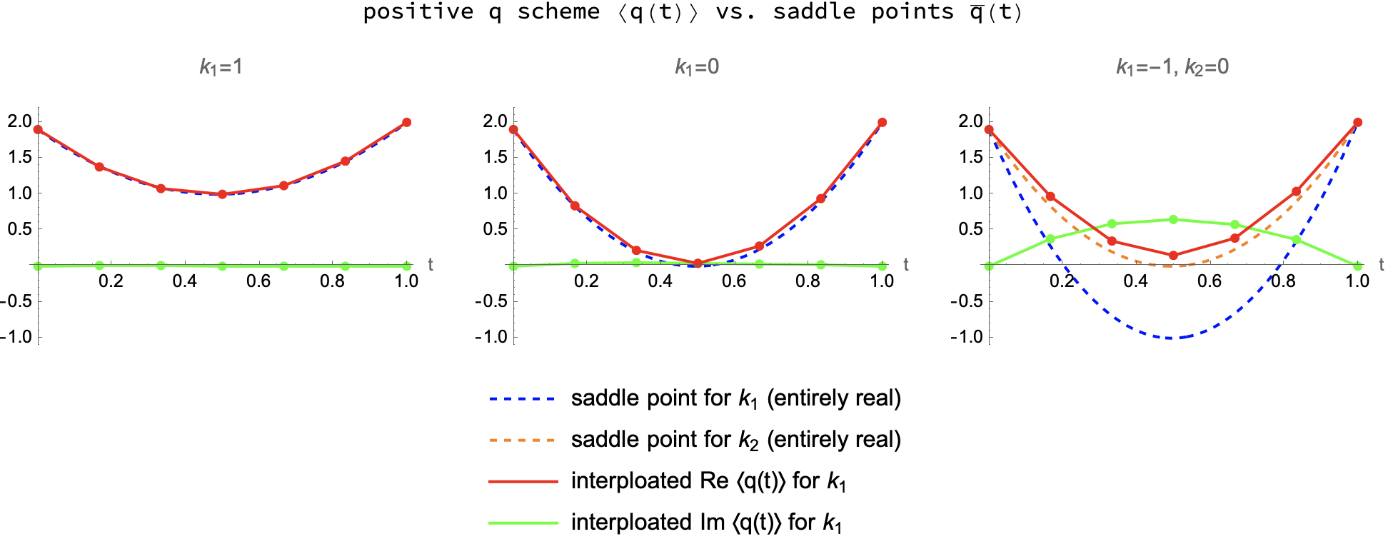
In Figure 2 we took and . For the same parameters, Figure 6 and Table 1 summarize the numerical results based on (27) with .
For and , the expectation values and from the positive and real schemes are close, as seen in Table 1. The expectation values are in turn close to the saddle point values , as seen from Figure 6. In particular, the imaginary part of the saddle points vanish, and the imaginary part of the expectation values are also close to zero. In contrast:
- •
For , the expectation values and from the positive and real schemes differ much. In the positive scheme, deviate much from which is real, and deviate much from zero.
Besides, there is a fundamental difference that applies to all values of . In the positive scheme all path integral configurations are Lorentzian, so we can compute expectation values for the comoving horizon (32) and its fluctuations as defined in Section V. In contrast, in the real scheme there are path integral configurations which are not Lorentzian, so the expectation value for the comoving horizon is undefined. The results for for the real scheme are shown in the last three columns of Table 1. To the extent that offers an indirect indicator of the amount of fluctuation:
- •
In the positive scheme, the amount of lightcone fluctuation as indicated by is much larger for than for and .
VI.3 Understanding the expectation values

In the first bullet point of Section VI.2, we noted that the real scheme expectation values for differ much from the saddle point values in the negative spatial curvature case. To understand this, it helps to consider again the one-variable toy model of Section III.2. According to Picard-Lefschetz theory Feldbrugge2017LorentzianCosmology, the real line approaches the steepest descent contour asymptotically under the holomorphic gradient flow defined by (16) and plotted in Figure 7.
In the real scheme, the integration contour is the real line. Since this contour is deformed into the steepest descent contour under the flow, and the integral can be equivalently performed there. As shown in Figure 7, the saddle point is at . Points around the saddle point along the steepest descent contour all have negative real parts around , but some have positive and some have negative imaginary parts. Therefore we expect to have a negative real part around the saddle point, and an almost vanishing or exactly vanishing imaginary part due to the cancellation from positive and negative contributions.
In the positive scheme, the integration contour is the positive halfline. As shown in Figure 7, this contour only approaches a portion of the steepest descent contour quite far from the saddle point. In particular, all points of the original contour flow towards the directions of positive real values and negative imaginary values. Therefore we expect to have a much larger real part than the saddle point, and a much smaller imaginary part than zero.
The actual model for we considered has more dynamical variables than one. However, similarly the real parts of deviate much from the negative saddle point values, and the imaginary parts of deviate much from zero (Figure 8). Presumably this is for the same reason that under the holomorphic gradient flow, the original positive contour approaches only a portion of the steepest descent contour which does not cover the saddle point.


VI.4 Understanding the fluctuations
From Table 1, we see that the lightcone fluctuation measurers and differ much among the cases. In addition, for the fluctuations in and differ much between the real and positive q schemes, as shown in Figure 8 vs. Figure 9. These difference can be understood better by drawing an analogy to a simpler setting.

Consider three Gaussian distributions with standard deviation , but centered around different locations and . Assume that only the portion along the positive real halfline is relevant, and rescale the distributions so that they are normalized on . As shown in Figure 10, the smaller is, the more sharply the distribution is peaked. As a consequence, the standard deviation computed on is smaller for smaller (Figure 10).
In the case of quantum cosmology, the real vs. positive schemes of is like vs. . In the real scheme, the original contour covers the whole steepest descent contour under the holomorphic gradient flow, and the magnitude of the integrand varies slowly around the saddle point to yield relatively large fluctuations. This is like the case where a large portion around the peak is covered by the positive domain. In the positive scheme, the original contour only covers a portion of the steepest descent contour under the holomorphic gradient flow. This portion does not contain the saddle point, and the magnitude of the integrand varies much faster around the peak that is covered. This is like the case where the peak lies far outside the positive domain. Therefore the fluctuations in and are smaller in comparison to the real scheme (Figure 8 vs. Figure 9).
The positive scheme of vs. is like vs. . For , the saddle point is on the boundary of the original contour. This is like the case where the peak is on the boundary of the positive domain. Here we expect more fluctuation than , which is analogous to the case where the peak lies far outside of the positive domain. This explains why there is more fluctuation for than for measured by , as noted in the second bullet point of Section VI.2.
Finally, there is also less fluctuation for than for as measured by . This is presumably because of the form of the comoving distance function (32). As approaches zero, becomes very large and very sensitive to the precise value of . Since in the case the saddle point value does get very close to zero, while in the case it does not, larger fluctuations in is expected.
VI.5 Breakdown of saddle point approximation
In previous works of quantum cosmology, it is common to apply saddle point approximation to the path integrals. Here in the example the saddle point failed at capturing the quantum expectation values of the truly Lorentzian path integral. This shows that the technique of saddle point semiclassical approximation does not enjoy universal validity for Lorentzian quantum cosmology, and must be used with caution.33 3 When naive saddle point approximation on unrestricted domain does break down, it may be interesting to develop new saddle point approximation method on bounded domains along the line of, e.g., Delabaere2002GlobalBoundaries.
VII Singularity avoidance
VII.1 Is singularity avoidance trivial?
Even when the expectation values are close (as in the case), the positive and real schemes still differ on the critical issue of singularity avoidance. There are many non-trivial ideas of singularities avoidance in quantum gravity. For example, through discreteness, nonlocality, higher-order terms in the action, final boundary condition choices etc. However, there is a trivial alternative. A gravitational path integral may simply not include singular spacetimes in its sum JiaIsTrivial; Suen1989WaveSystem.
For the minisuperspace model studied here, this indeed follows from including only Lorentzian configurations in the path integral. At the singularity, the metric (3) is of signature . This is not of the Lorentzian signature, so it is automatically avoided in the truly Lorentzian path integral. In this sense, singularity avoidance is trivially achieved.
VII.2 Tunnelling and no-boundary proposals
Interestingly, insisting on a strictly Lorentzian path integral for all time including invalidates from the outset Lorentzian variants of the tunnelling/no-boundary proposals that set . Therefore one must choose from: (1) allowing non-Lorentzian configurations in the path integral; or (2) rejecting boundary conditions that set to zero.
Choice (1) calls for some additional specifications. Suppose quantum cosmology is governed by some fundamental theory of quantum gravity. Then how exactly are non-Lorentzian configurations included in the path integral for this fundamental theory? Is non-Lorentzianess only allowed at certain places of quantum spacetime but not others? If so, at exactly which kind of places, and why not at other places? One possibility is to consider non-Lorentzian pieces at the boundary of superspace, and allow this kind of non-Lorentzianness in the path integral Vilenkin1988QuantumUniverse. However, this proposal needed to divide the boundary of superspace into regular and singular parts, and append additional rules associated with probability fluxes to these two parts. However, as far as we know the exact definition of the regular and singular parts of the boundary has never been written down in general Fanaras2022TheCosmology, and this proposal still remains as an incomplete idea.
Choice (2) is dynamically less ambiguous since no additional rule is needed on how to include non-Lorentzian configurations. However, it leaves open the question of boundary conditions which can only be determined by other means. One possibility is to impose an ordinary Lorentzian boundary condition concentrated around small positive values of . Another possibility is to give up on boundary conditions at small sizes of the universe and investigate boundary conditions for bouncing cosmology Brandenberger2017BouncingProblems.
VIII Discussions
Quantum cosmology based on Lorentzian path integrals is a promising avenue. However, many previous studies integrate the squared scale factor over the whole real line. This step introduces non-Lorentzian configurations into the path integral. Instead, a truly Lorentzian path integral should only include positive squared scale factor.
Here we studied and compared minisuperspace path integrals with real and positive squared scale factors. By restricting to Lorentzian configurations, the truly Lorentzian case enables the study of causal horizons and their quantum fluctuations, and achieves singularity avoidance by excluding singular minisuperspace geometries as non-Lorentzian. In addition, we find that the expectation values can differ much between the two cases. This happens in particular when the saddle point configuration does not belong to the strictly Lorentzian integration contour and is not connected to the strictly Lorentzian integration contour by the holomorphic gradient flow.
These results challenge the universal validity of saddle point approximation widely used in quantum cosmology. In particular this affects topics such as Lorentzian variations of tunnelling/no-boundary proposals, and the quantum completeness of inflation DiTucci2019QuantumInflation. In these cases, the saddle point gets close to or below zero, so that it does not belong to the strictly Lorentzian integration contour. Instead of using saddle point approximation, a safer option is to compute the path integral directly. This can be done, for example, using the generalized thimble method adopted here.
We finish by a discussion on some topics to be understood better.
VIII.1 Negative q
Although the metric (3) has the signature only when , it has the signature when . One may wonder whether this rescues the real scheme for a Lorentzian path integral, since the signature might also be considered Lorentzian.
However, an attempt at rescue face some outstanding issues, because the real scheme path integral includes configurations where at certain times and at other times.
First, such a configuration involves signature change. It does not qualify as a Lorentzian spacetime in the usual sense such that the spacetime stays within the or the signature.
Second, in connecting the and parts of the configuration has to cross . Here the metric has signature . This is not Lorentzian.
Third, when crosses , it is not a priori clear what the causal structure is for that spacetime. Some additional rules are required to tell how causal paths travel across the singularity at . Without such a rule, the causal relation between two events from the and parts of spacetime remains unclear.
VIII.2 Inhomogeneity, anisotropy, and matter coupling
The present study is restricted to minisuperspace models. For further research it is certainly interesting to accommodate inhomogeneity and/or anisotropy in the truly Lorentzian setting. For example, the Bianchi types I and III, and Kantowski-Sachs models studied in Halliwell1990Steepest-descentModels, and the biaxial Bianchi IX model studied in Dorronsoro2018DampedState; Feldbrugge2018InconsistenciesProposal may be simple enough as starting points to incorporate anisotropy. In a general non-perturbative setting, simplicial manifold models provide a systematic way to incorporate inhomogeneity and anisotropy in quantum cosmology Hartle1985SimplicialDiscussion; Hartle1986SimplicialTriangulations; Hartle1989SimplicalModel; Louko1992ReggeCosmology; Birmingham1995LensCosmology; Birmingham1998ACalculus; Furihata1996No-boundaryUniverse; Silva1999SimplicialField; Silva1999AnisotropicField; Silva2000SimplicialPhi2; daSilvaWormholesMinisuperspace. Traditionally, simplicial quantum gravity is studied with respect to an Euclidean contour or an ad hoc complex contour, but there has been growing attention towards the Lorentzian case Tate2011Fixed-topologyDomain; Tate2012Realizability1-simplex; Jia2022Time-spaceGravity; Jia2022ComplexProspects; Jia2022LightGravity; JiaLightGravity; JiaIsTrivial; Dittrich2022LorentzianSimplicial; AsanteComplexCosmology; Ito2022TensorCalculus. In particular, the generalized thimble method employed here and in Jia2022ComplexProspects may be applicable in studies of inhomogeneity and anisotropy.
Certainly one should also consider matter coupling in further works. In addition to coupling to scalar fields and investigate the inflation scenario, we also find alternative scenarios without inflation worth investigating Gielen2015PerfectBounce; BoyleTwo-SheetedTime; TurokGravitationalPuzzles; BoyleThermodynamicConstant.
VIII.3 Lightcone topics
Another topic about simplicial models of direct relevance is irregular lightcone structures. In simplicial models, there is the question whether the path integral should include simplicial geometries with interior points attached to more or fewer than two lightcones. In AsanteComplexCosmology; Dittrich2022LorentzianSimplicial this question is studied based on a comparison with the continuum minisuperspace model in the real scheme. It is worth revisiting this topic given that the positive scheme may yield a different result.
In Section VI, we noted that the case exhibit larger causal horizon fluctuations than the and cases. For the case, that the fluctuations are smaller is related to the breakdown of saddle point approximation based on Einstein’s equations. Whether this and other effects of lightcone fluctuations lead to any observable signatures is worth investigating further.
VIII.4 Singularity
Much of quantum cosmology is driven by the hope to understand singularities. In the recent wave of interest for Lorentzian quantum cosmology, the question has been raised whether singular geometries with should be avoided in the path integral DiTucci2019No-boundaryCosmology, as such geometries enter critical discussions about boundary conditions Feldbrugge2017NoProposal; DiTucci2018UnstableMetrics; DiTucci2019No-BoundaryConditions; DiTucci2019No-boundaryCosmology; Jonas2022RevisitingField and inflation Bramberger2019HomogeneousCosmology. In Section VII we showed that in a strictly Lorentzian path integral, singularities are automatically excluded as non-Lorentzian. How this affects the above topics is an open question.
There are many attempts to find effective regular spacetimes that replace spacetimes with cosmological and black hole singularities. Some of these derive regular solutions from equations of motion of modified actions. The example studied here shows that an effective singularity-free geometry that characterizes the quantum theory at leading order (e.g., gives the correct expectation values) need not obey the equation of motion from an action principle. It remains to be clarified how such alternative views on singularity avoidance stand to each other.
VIII.5 Analytic insights
In computing the oscillating complex path integrals, we applied the generalized thimble method Alexandru2016SignThimbles to overcome the numerical sign problem. This method would not have been available a decade ago. However, new methods for evaluating complex path integrals are being developed at a promising pace in the recent decade (see e.g., Alexandru2022ComplexProblem; Berger2019ComplexPhysics; Gattringer2016ApproachesTheory; CarmenBauls2020ReviewTheories and references therein). We expect such technical tools to boost the study beyond semiclassical analysis for the Lorentzian path integrals.
That said, it is still beneficial to find analytic methods to complement the numerical methods. One idea is to identify the value of so that the -dependent saddle point of (7) just falls within the Lorentzian domain. Flowing this pair of - values under the holomorphic gradient flow to the steepest descent contour may yield a close guess at the expectation values.
Acknowledgement
I am very grateful to Shengqi Sang, Latham Boyle, Niayesh Afshordi for helpful discussions, to Jean-Luc Lehners for friendly and informative comments on an earlier draft of the paper, and to Lucien Hardy and Achim Kempf for long-term encouragement and support. The numerical computation is conducted on Perimeter Institute’s Symmetry high-performance computing cluster. I thank Dustin Lang for helps with setting up the computation there. Research at Perimeter Institute is supported in part by the Government of Canada through the Department of Innovation, Science and Economic Development Canada and by the Province of Ontario through the Ministry of Economic Development, Job Creation and Trade.
References
- [1] H. W. Hamber. Quantum Gravitation: the Feynman Path Integral Approach. Springer, Berlin, 2009.
- [2] Jan Ambjorn. Quantization of Geometry. arXiv: hep-th/9411179.
- [3] Tullio Regge and Ruth M. Williams. Discrete structures in gravity. Journal of Mathematical Physics, 41(6):3964–3984, 12 2000.
- [4] Kyle Tate and Matt Visser. Fixed-topology Lorentzian triangulations: Quantum Regge Calculus in the Lorentzian domain. Journal of High Energy Physics, 2011(11):72, 11 2011.
- [5] Ding Jia. Time-space duality in 2D quantum gravity. Classical and Quantum Gravity, 39(3):035016, 1 2022.
- [6] J. Ambjørn and R. Loll. Non-perturbative Lorentzian quantum gravity, causality and topology change. Nuclear Physics B, 536(1-2):407–434, 12 1998.
- [7] Renate Loll. A Discrete History of the Lorentzian Path Integral. In Domenico J. W. Giulini, Claus Kiefer, and Claus Lämmerzahl, editors, Quantum Gravity: From Theory to Experimental Search, pages 137–171. Springer, Berlin, 2003.
- [8] Lee Smolin. Quantum gravity on a lattice. Nuclear Physics B, 148(3-4):333–372, 2 1979.
- [9] G. W. Gibbons. The Einstein action of Riemannian metrics and its relation to quantum gravity and thermodynamics. Physics Letters A, 61(1):3–5, 4 1977.
- [10] James B. Hartle. Simplicial minisuperspace I. General discussion. Journal of Mathematical Physics, 26(4):804–814, 4 1985.
- [11] James B. Hartle. Simplicial minisuperspace. II. Some classical solutions on simple triangulations. Journal of Mathematical Physics, 27(1):287–295, 1 1986.
- [12] James B. Hartle. Simplical minisuperspace. III. Integration contours in a five-simplex model. Journal of Mathematical Physics, 30(2):452–460, 2 1989.
- [13] Jonathan J. Halliwell and Jorma Louko. Steepest-descent contours in the path-integral approach to quantum cosmology. I. The de sitter minisuperspace model. Physical Review D, 39(8):2206–2215, 4 1989.
- [14] Jonathan J. Halliwell and Jorma Louko. Steepest-descent contours in the path-integral approach to quantum cosmology. II. Microsuperspace. Physical Review D, 40(6):1868, 9 1989.
- [15] Jonathan J. Halliwell and Jorma Louko. Steepest-descent contours in the path-integral approach to quantum cosmology. III. A general method with applications to anisotropic minisuperspace models. Physical Review D, 42(12):3997, 12 1990.
- [16] Jonathan J. Halliwell and Robert C. Myers. Multiple-sphere configurations in the path-integral representation of the wave function of the Universe. Physical Review D, 40(12):4011, 12 1989.
- [17] Jonathan J. Halliwell and James B. Hartle. Integration contours for the no-boundary wave function of the universe. Physical Review D, 41(6):1815, 3 1990.
- [18] Kristin Schleich. Semiclassical wave function of the Universe at small three-geometries. Physical Review D, 32(8):1889, 10 1985.
- [19] Kristin Schleich. Conformal rotation in Bianchi type-I quantum cosmology. Physical Review D, 39(8):2192, 4 1989.
- [20] Edward Farhi. The wave function of the universe and the square root of minus one. Physics Letters B, 219(4):403–407, 3 1989.
- [21] James M. Cline. Does the wormhole mechanism for vanishing cosmological constant work in lorentzian gravity? Physics Letters B, 224(1-2):53–57, 6 1989.
- [22] Wai Mo Suen and Kenneth Young. Wave function of the Universe as a leaking system. Physical Review D, 39(8):2201, 4 1989.
- [23] J. David Brown and Erik A. Martinez. Lorentzian path integral for minisuperspace cosmology. Physical Review D, 42(6):1931, 9 1990.
- [24] Job Feldbrugge, Jean-Luc Lehners, and Neil Turok. Lorentzian Quantum Cosmology. Physical Review D, 95(10), 3 2017.
- [25] Rafael D. Sorkin. Is the spacetime metric Euclidean rather than Lorentzian? In Arundhati Dasgupta, editor, Recent Research in Quantum Gravity, pages 115–135. Nova Science Publishers, New York, 2013.
- [26] J. Diaz Dorronsoro, J. J. Halliwell, J. B. Hartle, T. Hertog, and O. Janssen. Real no-boundary wave function in Lorentzian quantum cosmology. Physical Review D, 96(4):043505, 8 2017.
- [27] Job Feldbrugge, Jean-Luc Lehners, and Neil Turok. No smooth beginning for spacetime. Physical Review Letters, 119(17), 4 2017.
- [28] Job Feldbrugge, Jean-Luc Lehners, and Neil Turok. No Rescue for the No Boundary Proposal. Physical Review D, 97(2), 8 2017.
- [29] J. Diaz Dorronsoro, J. J. Halliwell, J. B. Hartle, T. Hertog, O. Janssen, and Y. Vreys. Damped Perturbations in the No-Boundary State. Physical Review Letters, 121(8):081302, 8 2018.
- [30] Job Feldbrugge, Jean Luc Lehners, and Neil Turok. Inconsistencies of the new no-boundary proposal. Universe, 4(10):100, 10 2018.
- [31] Alexander Vilenkin and Masaki Yamada. Tunneling wave function of the universe. Physical Review D, 98(6):066003, 9 2018.
- [32] Alice Di Tucci and Jean Luc Lehners. Unstable no-boundary fluctuations from sums over regular metrics. Physical Review D, 98(10):103506, 11 2018.
- [33] Alice Di Tucci, Job Feldbrugge, Jean-Luc Lehners, and Neil Turok. Quantum Incompleteness of Inflation. Physical Review D, 100(6), 6 2019.
- [34] Oliver Janssen, Jonathan J. Halliwell, and Thomas Hertog. The no-boundary proposal in biaxial Bianchi IX minisuperspace. Physical Review D, 99(12), 4 2019.
- [35] Alice Di Tucci and Jean Luc Lehners. No-Boundary Proposal as a Path Integral with Robin Boundary Conditions. Physical Review Letters, 122(20):201302, 5 2019.
- [36] Alice Di Tucci, Jean-Luc Lehners, and Laura Sberna. No-boundary prescriptions in Lorentzian quantum cosmology. Physical Review D, 100(12), 11 2019.
- [37] Sebastian F. Bramberger, Alice Di Tucci, and Jean-Luc Lehners. Homogeneous Transitions during Inflation: a Description in Quantum Cosmology. Physical Review D, 101(6), 7 2019.
- [38] Alice Di Tucci, Michal P. Heller, and Jean Luc Lehners. Lessons for quantum cosmology from anti-de Sitter black holes. Physical Review D, 102(8):086011, 10 2020.
- [39] Gaurav Narain and Hai-Qing Zhang. Lorentzian quantum cosmology in novel Gauss-Bonnet gravity from Picard-Lefschetz methods. arXiv: 2006.02298.
- [40] Karthik Rajeev, Vikramaditya Mondal, and Sumanta Chakraborty. No-boundary Wave Function, Wheeler-DeWitt Equation and Path Integral Analysis of the Bouncing ‘Quantum’ Cosmology. Physical Review D, 103(10), 1 2021.
- [41] Karthik Rajeev, Vikramaditya Mondal, and Sumanta Chakraborty. Bouncing with shear: Implications from quantum cosmology. Journal of Cosmology and Astroparticle Physics, 2022(1), 9 2021.
- [42] Jean-Luc Lehners. The Wave Function of Simple Universes, Analytically Continued From Negative to Positive Potentials. Physical Review D, 104(6), 5 2021.
- [43] Gaurav Narain. On Gauss-Bonnet gravity and boundary conditions in Lorentzian path-integral quantization. Journal of High Energy Physics 2021 2021:5, 2021(5):1–35, 5 2021.
- [44] Jean Luc Lehners. Allowable complex metrics in minisuperspace quantum cosmology. Physical Review D, 105(2):026022, 1 2022.
- [45] Caroline Jonas, Jean-Luc Lehners, and Vincent Meyer. Revisiting the no-boundary proposal with a scalar field. Physical Review D, 105(4):043529, 2 2022.
- [46] Hiroki Matsui. Lorentzian path integral for quantum tunneling and WKB approximation for wave-function. The European Physical Journal C 2022 82:5, 82(5):1–16, 5 2022.
- [47] Gaurav Narain. Surprises in Lorentzian path-integral of Gauss-Bonnet gravity. Journal of High Energy Physics 2022 2022:4, 2022(4):1–27, 4 2022.
- [48] Caroline Jonas, Jean-Luc Lehners, and Jerome Quintin. Uses of complex metrics in cosmology. Journal of High Energy Physics 2022 2022:8, 2022(8):1–39, 8 2022.
- [49] Jonathan J. Halliwell. Derivation of the Wheeler-DeWitt equation from a path integral for minisuperspace models. Physical Review D, 38(8):2468, 10 1988.
- [50] Ding Jia. Is singularity resolution trivial? arXiv: 2204.12304.
- [51] Andrei Alexandru, Gökçe Basar, Paulo F. Bedaque, Gregory W. Ridgway, and Neill C. Warrington. Sign problem and Monte Carlo calculations beyond Lefschetz thimbles. Journal of High Energy Physics 2016 2016:5, 2016(5):1–17, 5 2016.
- [52] James W. York. Role of conformal three-geometry in the dynamics of gravitation. Physical Review Letters, 28(16):1082–1085, 4 1972.
- [53] G. W. Gibbons and S. W. Hawking. Action integrals and partition functions in quantum gravity. Physical Review D, 15(10):2752–2756, 5 1977.
- [54] Richard P. Feynman and Albert R. Hibbs. Quantum Mechanics and Path Integrals. McGraw-Hill, New York, 1965.
- [55] Alexander Vilenkin. Creation of universes from nothing. Physics Letters B, 117(1-2):25–28, 11 1982.
- [56] Alexander Vilenkin. Quantum creation of universes. Physical Review D, 30(2):509–511, 7 1984.
- [57] A. D. Linde. Quantum creation of the inflationary universe. Lettere al Nuovo Cimento, 39(17):401–405, 4 1984.
- [58] J. B. Hartle and S. W. Hawking. Wave function of the Universe. Physical Review D, 28(12):2960–2975, 12 1983.
- [59] Ding Jia. Light ray fluctuations in simplicial quantum gravity. Classical and Quantum Gravity, 39(13):135005, 6 2022.
- [60] Aurélien Barrau, Killian Martineau, and Flora Moulin. Seeing through the cosmological bounce: Footprints of the contracting phase and luminosity distance in bouncing models. Physical Review D, 96(12):123520, 12 2017.
- [61] Andrei Alexandru, Gökçe Başar, Paulo F. Bedaque, Gregory W. Ridgway, and Neill C. Warrington. Monte Carlo calculations of the finite density Thirring model. Physical Review D, 95(1):014502, 1 2017.
- [62] AuroraScience Collaboration, Marco Cristoforetti, Francesco Di Renzo, and Luigi Scorzato. High density QCD on a Lefschetz thimble? Physical Review D - Particles, Fields, Gravitation and Cosmology, 86(7), 5 2012.
- [63] Andrei Alexandru, Gökçe Başar, Paulo F. Bedaque, and Neill C. Warrington. Complex paths around the sign problem. Reviews of Modern Physics, 94(1):015006, 3 2022.
- [64] Andrei Alexandru, Gokce Basar, Paulo F. Bedaque, and Neill C. Warrington. Tempered transitions between thimbles. Physical Review D, 96(3), 3 2017.
- [65] Masafumi Fukuma and Naoya Umeda. Parallel tempering algorithm for integration over Lefschetz thimbles. Progress of Theoretical and Experimental Physics, 2017(7), 3 2017.
- [66] Masafumi Fukuma and Nobuyuki Matsumoto. Worldvolume approach to the tempered Lefschetz thimble method. Progress of Theoretical and Experimental Physics, 2021(2):23–31, 2 2021.
- [67] Genki Fujisawa, Jun Nishimura, Katsuta Sakai, and Atis Yosprakob. Backpropagating Hybrid Monte Carlo algorithm for fast Lefschetz thimble calculations. Journal of High Energy Physics, 2022(4):1–27, 4 2022.
- [68] Jeff Bezanson, Alan Edelman, Stefan Karpinski, and Viral B. Shah. Julia: A Fresh Approach to Numerical Computing. SIAM Review, 59(1):65–98, 2 2017.
- [69] Christopher Rackauckas, Anshul Singhvi, Yingbo Ma, Chris de Graaf, Lilith Orion Hafner, Michael Hatherly, Scott P. Jones, dextorious, Arno Strouwen, Colin Caine, Elliot Saba, Julia TagBot, Kvaz1r, Max G, Sam Isaacson, Sheehan Olver, The Gitter Badger, c123w, and Maja Gwóźdź. SciML/DifferentialEquations.jl: v7.3.0. 8 2022.
- [70] Ding Jia. Complex, Lorentzian, and Euclidean simplicial quantum gravity: numerical methods and physical prospects. Classical and Quantum Gravity, 39(6):065002, 2 2022.
- [71] Gareth O. Roberts and Jeffrey S. Rosenthal. Examples of Adaptive MCMC. Journal of Computational and Graphical Statistics, 18(2):349–367, 2009.
- [72] Ding Jia. Light ray fluctuation and lattice refinement of simplicial quantum gravity. Classical and Quantum Gravity, 40(16):165003, 2023.
- [73] Eric Delabaere and C. J. Howls. Global asymptotics for multiple integrals with boundaries. Duke Mathematical Journal, 112(2):199–264, 4 2002.
- [74] Alexander Vilenkin. Quantum cosmology and the initial state of the Universe. Physical Review D, 37(4):888, 2 1988.
- [75] Georgios Fanaras and Alexander Vilenkin. The tunneling wavefunction in Kantowski-Sachs quantum cosmology. Journal of Cosmology and Astroparticle Physics, 2022(08):069, 8 2022.
- [76] Robert Brandenberger and Patrick Peter. Bouncing Cosmologies: Progress and Problems. Foundations of Physics 2017 47:6, 47(6):797–850, 2 2017.
- [77] J Louko and P A Tuckey. Regge calculus in anisotropic quantum cosmology. Classical and Quantum Gravity, 9(1):41, 1 1992.
- [78] Danny Birmingham. Lens spaces in the Regge calculus approach to quantum cosmology. Physical Review D, 52(10):5760, 11 1995.
- [79] Danny Birmingham. A Closed Contour of Integration in Regge Calculus. General Relativity and Gravitation 1998 30:1, 30(1):83–103, 1998.
- [80] Yasuhiko Furihata. No-boundary wave function for a simplicial anisotropic universe. Physical Review D, 53(12):6875, 6 1996.
- [81] Cristóvão Correia da Silva and Ruth M Williams. Simplicial minisuperspace models in the presence of a scalar field. Classical and Quantum Gravity, 16(7):2197, 7 1999.
- [82] Cristóvão Correia da Silva and Ruth M Williams. Anisotropic simplicial minisuperspace model in the presence of a scalar field. Classical and Quantum Gravity, 16(8):2681, 8 1999.
- [83] Cristóvão Correia da Silva and Ruth M Williams. Simplicial minisuperspace models in the presence of a massive scalar field with arbitrary scalar coupling eta R phiˆ2. Classical and Quantum Gravity, 17(8):1827, 4 2000.
- [84] Cristovao Correia da Silva and Ruth M. Williams. Wormholes in Simplicial Minisuperspace. arXiv: gr-qc/0004035.
- [85] Kyle Tate and Matt Visser. Realizability of the Lorentzian (n, 1)-simplex. Journal of High Energy Physics, 2012(1):28, 1 2012.
- [86] Bianca Dittrich, Steffen Gielen, and Susanne Schander. Lorentzian quantum cosmology goes simplicial. Classical and Quantum Gravity, 39(3):035012, 1 2022.
- [87] Seth K. Asante, Bianca Dittrich, and José Padua-Argüelles. Complex actions and causality violations: Applications to Lorentzian quantum cosmology. Classical and Quantum Gravity, 40(10):105005, 2023.
- [88] Yoshiyasu Ito, Daisuke Kadoh, and Yuki Sato. Tensor network approach to 2D Lorentzian quantum Regge calculus. Physical Review D, 106(10):106004, 11 2022.
- [89] Steffen Gielen and Neil Turok. Perfect Quantum Cosmological Bounce. Physical Review Letters, 117(2), 10 2015.
- [90] Latham Boyle and Neil Turok. Two-Sheeted Universe, Analyticity and the Arrow of Time. arXiv:2109.06204.
- [91] Neil Turok and Latham Boyle. Gravitational entropy and the flatness, homogeneity and isotropy puzzles. arXiv:2201.07279.
- [92] Latham Boyle and Neil Turok. Thermodynamic solution of the homogeneity, isotropy and flatness puzzles (and a clue to the cosmological constant). arXiv:2210.01142.
- [93] Casey E. Berger, Lukas Rammelmüller, Andrew C. Loheac, Florian Ehmann, Jens Braun, and Joaquín E. Drut. Complex Langevin and other approaches to the sign problem in quantum many-body physics. Physics Reports, 892:1–54, 7 2019.
- [94] Christof Gattringer and Kurt Langfeld. Approaches to the sign problem in lattice field theory. International Journal of Modern Physics A, 31(22):1643007–, 3 2016.
- [95] Mari Carmen Bauls and Krzysztof Cichy. Review on novel methods for lattice gauge theories. Reports on Progress in Physics, 83(2):024401, 1 2020.