2022
The COVID-19 pandemic has caused over 6.4 million registered deaths to date and has had a profound impact on economic activity. Here, we study the interaction of transmission, mortality, and the economy during the SARS-CoV-2 pandemic from January 2020 to December 2022 across 25 European countries. We adopt a Bayesian Mixed Effects model with auto-regressive terms. We find that increases in disease transmission intensity decreases Gross domestic product (GDP) and increases daily excess deaths, with a longer lasting impact on excess deaths in comparison to GDP, which recovers more rapidly. Broadly, our results reinforce the intuitive phenomenon that significant economic activity arises from diverse person-to-person interactions. We report on the effectiveness of non-pharmaceutical interventions (NPIs) on transmission intensity, excess deaths, and changes in GDP, and resulting implications for policy makers. Our results highlight a complex cost-benefit trade off from individual NPIs. For example, banning international travel increases GDP and reduces excess deaths. We consider country random effects and their associations with excess changes in GDP and excess deaths. For example, more developed countries in Europe typically had more cautious approaches to the COVID-19 pandemic, prioritising healthcare, and excess deaths over economic performance. Long term economic impairments are not fully captured by our model, as well as long term disease effects (Long Covid). Our results highlight that the impact of disease on a country is complex and multifaceted, and simple heuristic conclusions to extract the best outcome from the economy and disease burden are challenging.
The interaction of transmission, mortality, and the economy: a retrospective analysis of the COVID-19 pandemic
keywords
Public health intervention, non-pharmaceutical interventions, economic impact assessment, COVID-19, SARS-CoV-21 Introduction
As of August 2022, there have been over 580 million registered COVID-19 cases globally with over 6.4 million registered deaths who_dashboard. However, these official counts substantially underestimate true COVID-19 disease burden Whittaker2021; Knutson2022. The pandemic prompted the largest vaccination campaign in history Tatar2021-xq with over 12.3 billion doses administered by August 2022 who_dashboard. The pandemic had a profound impact globally due in part to the largely unprecedented scale of non-pharmaceutical interventions (NPIs) to control transmission. The effect of NPIs on SARS-CoV-2 community transmission has been studied in detail, for example liu2021; haug2020ranking; mendez2021systematic; sera2021cross; brauner_npi; sharma2021understanding; flaxman2020estimating; banholzer2022estimating. Countries implemented NPIs, pharmaceutical interventions and economic support at different times and with differing individual specifications, allowing for a natural experiment to study their impact rosen2021pandemic. It is of critical importance to understand how various suites of interventions affected individual countries’ economic outlook and recovery.
The interaction between the pandemic and the economy have primarily been studied through two frameworks. The first framework integrates epidemiological models with economic models, and stratifies the population, often by its types of economic activity (e.g. economic sector, work-from-home vs. in-person etc.), typically for a single country. Smith et al Smith_2009 is an early example of a Computable General Equvilibrium (CGE) model. The authors studied the interaction between school closures, vaccination and the economy during pandemic influenza in the UK in 2009, relative to a baseline scenario of no mitigations. These studies have focused less on estimating economic impacts of the pandemic, and more on exploring potential interactions between disease spread, policy interventions and the economy under a range of assumptions and hypotheses (e.g. deb2021; Eichenbaum2020; alvarez2021; acemoglu2021). A minority of studies, e.g, haw2022optimizing, estimate epidemiological parameters by fitting models to epidemic data. This approach is useful to study counterfactual scenarios and the impact of potential interventions, while assuming the dynamics that are imposed on the system. Integrated Epidemiological Economic models predate the COVID-19 pandemic, but have received increased focus due increased data availability, the number of countries and diversity of data. Several studies, such as Fenichel et al Fenichel_2011, have focused on behavioural responses of individuals, and the models used in these studies tend to be highly mechanistic.
A second approach has been to estimate the interactions between transmission dynamics and the economy using statistical models, fitted to observational data, often from multiple countries. Longitudinal (panel) regression models have estimated the associations between economic variables, epidemiological variables and non-pharmaceutical restrictions. A variety of proxies have been used for economic variables, for example in godoy2022; verschuur2021; deb2021.
A small number of studies have used vector auto-regressive (VAR) models that incorporate temporal dynamics of the response variables, such as leibovici2022; jorda2022. brodeur2021 provides a more comprehensive literature review on the economics of the COVID-19 crisis.
Here we develop a holistic framework which models the interaction between COVID-19 transmission, NPIs and economic outcomes. We consider four response variables: natural logarithm of 1 + excess deaths per 100,000 population (labelled ), weekly change in GDP (on a scale whereby a unit change represents a tenth of the change in GDP), weekly change in transit measured via Google mobility data (scaled such that a transit level of 1 corresponds to the baseline level prior to 6 February 2020), and the logarithm of (as a measure of disease transmission intensity). To jointly model the correlations within and between response variables we use a VAR model, which allows us to model temporal dynamics for each response variable. Within the VAR framework we consider NPIs as exogenous (fixed effects) variables, (we discuss this modelling choice in section 4.4). The NPI data we use is highly heterogeneous across countries and over time, and this allows us to study the efficacy of these measures across the pandemic, controlling for both vaccinations and SARS-CoV-2 variants. NPIs were imposed by policy makers to control disease spread, but we also consider their broader behavioural and economic impact. The results reveal that each country needs to establish a balance of interventions given competing objectives and constraints they may face. We extend existing models to explore the dynamics of the above variables, in order to understand different policy responses and interventions during the pandemic.
A key challenge of modelling the pandemic and the economy in tandem is that we observe data at different levels of aggregation, subject to differing lags in reporting. Epidemiological data is typically available at a daily or weekly frequency whereas most economic data is generally available quarterly or annually. We make use of a number of non-standard data sets and modelling techniques to overcome this problem. The GDP data we use infers the changes in GDP between official announcements and is provided by an OECD model oecdeco, which matches official data closely.
We focus on 25 European countries for which high quality weekly data are available. Our analysis spans 2020-2021 to generate a holistic picture of the pandemic’s impact, which is not possible if considering only a single response variable (e.g. infection) or limited time period (e.g. the emergence and initial spread of SARS-CoV-2 in early 2020). We stop our analysis at the end of 2021 because other economic factors began to dominate in early 2022, most notably factors driving inflation and economic activity, which were independent of COVID-19.
2 Results

The conceptual framework of our study is summarised in Figure 1. A detailed description of the data and the model are available in section 4. A full list of parameter estimates is provided in Tables S4 to S8 in the Supplementary Information.
We assess the temporal relationships between response variables firstly using regression coefficients of the VAR component of the model, and secondly using the impulse response functions, as summarised in Figure 2. We provide the Identification Strategy in section 4.3.
The most significant coefficients of the model were the auto-regressive coefficients of the response variables with themselves, lagged by one time unit (i.e. one week). The coefficients for and were 0.856 (95% CrI: 0.828-0.884) and 0.757 (95% CrI: 0.725-0.790) respectively (Figure 2 B), indicating generally slow changes in those variables. The autoregressive coefficient for GDP was much lower (0.046, 95% CrI: -0.008 to 0.100), indicating that GDP varies substantially over short time periods. For Transit a negative autoregressive coefficient of -0.113 (95% CrI: -0.163 to -0.063) indicates compensatory corrective behaviour.
We estimate a positive coefficient between and lagged of 0.271 (95% CrI: 0.213-0.329), representing, as expected, a positive correlation between deaths and transmission intensity. A positive coefficient between and lagged Transit of 0.103 (95% CrI: 0.019-0.187) shows that mobility is associated with transmission intensity, as infections arise from previous person-to- person interaction. The positive coefficient between Transit and lagged GDP of 0.135 (95% CrI: 0.115 to 0.156) suggests that individuals adjust their mobility behaviour as a function of past economic activity.
We estimate negative coefficients between GDP and lagged (-0.241, 95% CrI: -0.295 to -0.189) and between Transit and lagged (-0.055, 95% CrI: -0.074 to -0.036), indicating that transmission intensity depresses both GDP and mobility. Interestingly, we estimate small but significant negative coefficients between both and lagged (-0.040, 95% CrI: -0.054 to -0.026) and between Transit and lagged (-0.025, 95% CrI: -0.033 to -0.018), suggesting increases in excess deaths prompt some decrease in mobility and transmission, independently of interventions.

To analyse the effects of coefficients on the overall dynamics of the model, we evaluate impulse response functions lutkepohl1990; pesaran1998generalized. Impulse response functions represent the change over time in three of the response variables due to a unit impulse (shock) in the fourth (Figure 2C). We find that a positive impulse in leads to a prolonged and significant increase in , which peaks after 5 weeks and only decays slowly. A positive impulse in also leads to a negative response in GDP and a similar if smaller impact on Transit, both of which peak after two weeks. Responses to impulses in the other response variables are consistent with coefficient estimates in Figure 2A, but are relatively small in absolute terms, even when significant.
All impulses ultimately converge to zero but convergence is slowest for excess deaths, followed by (as shown by the plots on the diagonal of Figure 2C), due to these variables’ high auto-regressive coefficient estimates.
We observe heterogeneities in NPIs across countries and time (Figure S6). In our VAR model, we include NPIs as predictor variables in two ways: the numerical level (stringency) of NPIs in each week, which we label as [level], and the change in that level from the previous week, which we label as [changes], (Tables S1,S2,S3). We found that the inclusion of both the level and change in level improves model performance. We used Leave-One-Out cross-validation (LOO-CV) to estimate the pointwise out of sample prediction accuracy from our fitted Bayesian model vehtari2017practical. The model with both levels and changes in NPIs outperformed a model with only levels of NPIs, with a expected log pointwise predictive density difference (ELPD-diff) of -80.9 (95% CrI: -136.1 to -25.7). Our preferred model, and the model with only changes in level included (ELPD-diff of -23.8 (95% CrI: -54.8 to 7.2)), are not statistically different. We prefer the model with both changes and levels of NPIs as it allows us to explain the effect of NPIs more fully.
Figure 3 shows estimated VAR model regression coefficients for NPI variables. Restrictions in workplace closure [changes] were statistically significant and associated with reductions in Transit (-0.026, 95% CrI: -0.036 to -0.017). Workplace closure restrictions [level] were associated with reduced (-0.012, 95% CrI: -0.021 to -0.003), indicating such closures led to a reduction of person to person contact rates.
Restrictions on gatherings [level] were associated with reductions in (-0.006, 95% CrI: -0.012 to -0.001), similarly to work place closures [level] (-0.012, 95% CrI: -0.021 to -0.003). Restrictions on gatherings [changes] were associated with an increase in (0.021, 95% CrI: 0.003-0.039).
International travel restrictions [changes] were associated with statistically significant reductions of Transit (-0.030, 95% CrI: -0.038 to -0.021), and with reductions [level] in (-0.014, 95% CrI: -0.028 to -0.001). The association of and international travel restrictions [level] (0.014, 95% CrI: 0.002 to 0.025), which also is significant for excess deaths [level] (-0.014, 95% CrI: -0.028 to -0.001), is consistent with Clifford et al clifford2021strategies, who discusses the effectiveness of different strategies of international travel restrictions, as those restrictions can slow down the importation of SARS-CoV-2 while allowing for a more open economy.
School Closure [changes] and closure of public transport [changes] were both associated with reductions in Transit. “Protecting the elderly” [changes] (-0.049, 95% CrI: -0.071 to -0.027) and “Schools Closing” (-0.026, 95% CrI: -0.049 to -0.003) [changes] NPIs were associated with reductions in GDP. “Protecting the elderly” [level] (-0.007, 95% CrI: -0.013 to -0.000) was associated with a reduction in .
Several NPI levels had positive and significant associations with GDP, in addition to International travel controls, Facial coverings [level] (0.016, 95% CrI: 0.007 to 0.026), Protection of elderly people [level] (0.015, 95% CrI: 0.005 to 0.027) and Income support [level] (0.023, 95% CrI: 0.009 to 0.039). Each of these measures allow for a more open economy. In the case of Income support individuals were able to isolate, thus reducing transmission risk (as Income support itself is a transfer payment by governments and hence not adding to GDP).
Facial coverings [level] were associated with increases in both (0.01, 95% CrI: 0.004-0.015) and (0.011, 95% CrI: 0.000-0.021). Facial coverings reduce the risk of infection, however as contacts increase we still see a net increase in infections and subsequent excess deaths.
We included the dominant SARS-CoV-2 variant in our model (wild-type, Alpha, Delta and Omicron), together with the average number of vaccine doses received per capita, allowing the latter to vary by variant. Tables S7 and S8 give estimates of the corresponding model parameters.
The variant coefficient for was significantly positive in the Delta and Omicron periods, and negative in the Alpha period. Stringent NPIs (e.g. gathering restrictions, workplace closures, school closures) were in place throughout most of Europe from December 2020 to May 2021, which likely accounts for the negative coefficients which we see for Alpha (Figures S6 and S9). Note we consider time periods over which there was a single dominant variant, and therefore differences between periods do not relect epidemiological characteristics of the variant itself.
For , the dominant variant had a significantly positive coefficient for the wild-type period, with smaller and non-significant coefficients for Alpha and Delta periods. The lower coefficient during the Alpha period is attributable to stringent NPIs, particularly high restrictions for isolating the elderly, and the initial vaccine roll-out. The elderly and those at higher risk of severe disease and death were prioritised, which likely affected both the Alpha and Delta periods. We estimate a large negative coefficient during the Omicron period, which is not quite significant at the 95% level, probably because the Omicron period in the data was short. Variant is negatively associated with GDP for the wild-type and Alpha, but positively associated for the Delta and Omicron periods, suggesting adaptation of the economy as COVID-19 restrictions eased. This adaption is a combination of easing of restrictions, businesses learning to operate during the pandemic with increased flexibility and time varying adherence to NPIs by individuals petherick2021worldwide.
Transit has positive coefficients for the Alpha period (0.013, 95% CrI: 0.004-0.022), driving by the rebound in mobility during the first half of 2021, and negative coefficients during for Omicron (-0.050, 95% CrI: -0.092 to -0.009) driven reduced mobility in the final months of 2021.
Vaccination was negatively associated with (-0.047, 95% CrI: -0.092 to -0.002), indicating its primary role in reducing mortality, and Transit (-0.02, 95% CrI: -0.033 to -0.005). Vaccination was not significantly associated with or GDP. The lack of significant association with GDP is because vaccination was only rolled out in 2021, and initially focused on the elderly and vulnerable, and not the working age population who make the largest contribution to economic activity, consistent with sonabend2021non which studies this for the Delta variant in England.
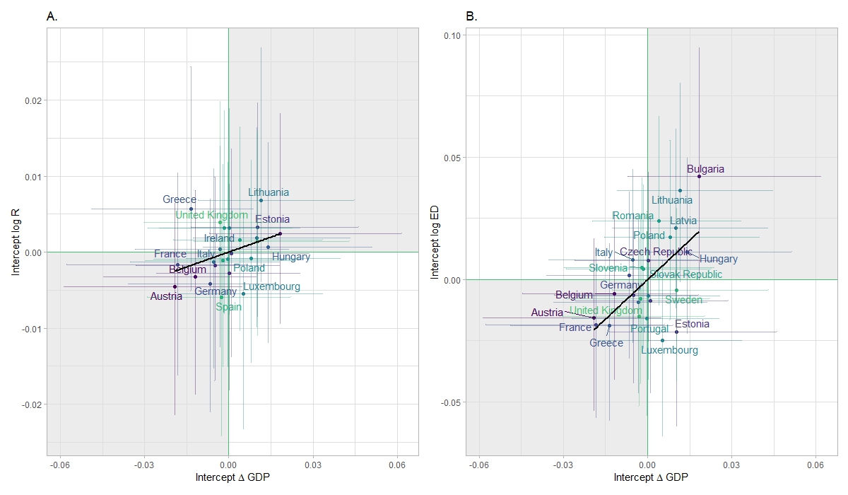
Countries had varied responses over the course of the pandemic. Eastern European countries imposed rigorous NPIs in March 2020 but less so from late 2020 onwards, compared with many Western European countries S7. Our model included country specific intercepts as random effects to represent residual variation after having taken account of all other “known” factors (that is, a positive intercept for in one country indicates a higher than average over the time period). Figure S15 shows the variation across countries for all response variables. There is only minor unexplained variability in Transit compared with the other three response variables. The ordering of countries for excess deaths and transmission intensity are broadly in line, however there is some change in the rank-order due to differences in healthcare systems.
We find a positive correlation between GDP and country intercepts (0.23, 95% CrI: -0.21 to 0.59 (Figure 4B), suggesting some trade-off between pandemic mortality and GDP that is independent of interventions (i.e. factors like behavioural changes). GDP and country intercepts also have positive correlation (0.09, 95% CrI: -0.33 to 0.46, see Figure 4A).
We consider the effect of country-specific intercept parameters on country characteristics. We include several characteristics across Government, economic, Household and Healthcare, as listed in Table 4.1. Resulting correlations are summarised in Figure 4C and listed in full in Table S10. For , we find positive correlations for the proportion of households with members over 60, Poverty rates, and Infant mortality per 1000 live births. Similarly we find negative correlations between the intercept and: Life expectancy at birth; access to financial institution accounts; Control of corruption; Individuals using the internet; Rule of Law; Infectious Disease vulnerabilty; the first principal component of 6 Government effectiveness indices; Human Develepmeny Index; Government effectiveness percentile rank; proportion of jobs that are teleworkable, and Freedom House global freedom score.
The intercept is negatively correlated with: Health expenditure as a fraction of GDP; life expectancy at birth; and Proportion of the population Living within 60min of an Urban Centre (Figure S16) at the 80% CrI. Therefore, countries with higher health expenditure had lower changes in GDP. The country-specific intercepts for and were not significantly correlated with any country-level characteristics we examined (Figure S17)
We consider different approaches to dimensional reduction and clustering of the country specific characteristics in the supplementary information B.6.
We are interested in the causal relationships of our response variables. Clearly, a cause cannot precede its the effect. If a variable affects another variable , the former should help improve the predictions of the latter. We again use LOO-CV to estimate the pointwise out-of-sample prediction accuracy from our fitted model. We systematically remove predictive variables from the model: if variable x is removed, it is removed from all equations, except the equation of x on itself (e.g. removing removes it from the right hand side of the equations of , GDP and Transit, but not the right hand side of itself). We do this for each response variable individually, all combinations of two response variables and removing all response variables (in which case each variable uses only itself). The results are summarised in Table 1, ordered by decreasing expected log pointwise predictive density (ELPD) difference.
The full model containing all variables has the best ELPD, although models excluding Transit, GDP or both of these are not statistically different at the 95% level from the full model. Excluding or , and any combination containing these predictors, the difference is statistically significant. is the most important predictive variable, as it leads to the largest negative ELPD differences, either on its own (compared to other single variable exclusions) or in combination with other variables excluded. Excluding all variables, so that each response variable is a function of only its past observations, leads to the largest ELPD negative difference indicating the worst performing model with respect to sample prediction accuracy. Together with the above vector-autoregressive coefficient estimates and the impulse response function, we have further evidence that transmission intensity increases excess deaths and negatively changes GDP.
| \topruleExcluded Variable | ELPD-diff | SE-diff | CrI Lower Bound | CrI Upper Bound |
|---|---|---|---|---|
| \midruleFull Model | 0.000 | 0.000 | 0.000 | 0.000 |
| Transit | -5.690 | 4.685 | -15.060 | 3.681 |
| GDP | -9.984 | 5.896 | -21.777 | 1.808 |
| GDP & Transit | -14.264 | 7.387 | -29.039 | 0.511 |
| -40.741 | 10.350 | -61.440 | -20.042 | |
| & Transit | -48.823 | 11.441 | -71.706 | -25.941 |
| GDP & | -51.353 | 12.469 | -76.291 | -26.415 |
| -69.044 | 13.484 | -96.012 | -42.076 | |
| & Transit | -73.989 | 14.424 | -102.837 | -45.140 |
| GDP & | -84.924 | 14.819 | -114.563 | -55.286 |
| & | -117.163 | 18.069 | -153.301 | -81.026 |
| All Variables | -145.501 | 20.373 | -186.248 | -104.754 |
| \bottomrule |
To further assess the predictive performance of our model, we compare the 1-timestep ahead forecast from our model to the naive forecast, which assumes the next value of a response variable is the same as its current value, that is . We find that our model improves predictions of all response variables, with a reduction of root mean squared error of 8% for transmission intensity, 6% for excess deaths, 27% for GDP and 32% for Transit (Figure S20). The improvements are due to improved forecasts in the tail of the distributions as opposed to the centre. This is expected, as the centre represents relatively stationary time periods. The model however does not have any awareness of e.g. holiday effects or other exogenous dynamics, and hence does not outperform the naive forecast during these periods. In the tails, i.e. during periods of high transmission intensity, the model performs better than the naive forecast.
3 Discussion
The interplay between transmission intensity, excess deaths, population mobility and GDP are highly complex, and cannot be considered in isolation. Here, we study their interaction holistically, for 25 European countries, during the first two years of the SARS-CoV-2 pandemic. Higher transmission intensity decreased GDP and increased excess deaths. Intensified public health interventions reduced mobility, transmission intensity, excess deaths and GDP. However, as our estimates allow for asymmetric relationships, changes in GDP alone (independent of control measures) were seen to have no significant impact on either transmission intensity or excess deaths. These findings generalise and extend results from previous studies leibovici2022, and make them more robust. Broadly, our results reinforce the intuitive phenomenon that significant economic activity arises from person-to-person interaction. Reductions in such interactions - by governmental mandate or behavioural change - reduce transmission, but also harm economic activity.
NPIs affect transmission, GDP and excess deaths in a variety of ways, but often act differently to each other. International travel restrictions reduce excess deaths, but increase economic activity, as more domestic activity can take place where importation of the virus is slowed due to quarantine, testing or outright travel bans clifford2021strategies. As found previously sharma2021understanding, workplace closures are associated with reductions in transmission intensity. As highlighted further below, we also find that specific economic characteristics of each country reduce transmission intensity. For example, countries with more face-to-face service sectors have higher transmission intensity (see Table S10).
Facial coverings (masks of all types) are an important intervention, as their societal costs and impacts are relatively small and no future economic costs are associated with facial coverings leech2022mask. Economically, facial coverings allow for greatly more open societies, and therefore economic activity. The impact of facial coverings on transmission intensity and excess deaths is more difficult to assess, as this is a function of adherence and face covering quality. We see positive associations between facial coverings (or mask mandates), and both excess deaths and transmission intensity. This may seem counter-intuitive, but can be regarded as a net effect of re-opening. While face masks allow increased social contact, and protect against transmission (albeit imperfectly), their adoption, concurrent with the easing of social distancing that they allow, can increase transmission and therefore excess deaths. Here, we do not assess the adherence to mask wearing by individuals, and only consider the policy.
Income support is an important intervention but direct interpretation of this coefficient requires caution. Income support itself is a government transfer payment which has no impact on GDP. The positive coefficient which we observe in the model with respect to GDP is the indirect result from two effects. First, income support enables individuals to continue to consume, even if they cannot work. Second, it enables businesses to continue to employ staff and maintain basic functions through the most significant restrictions, so that they can restart activity as soon as possible.
The behavioural response of individuals is an important component. Fenichel et al Fenichel_2011 used a highly mechanistic model to estimated the impact of behaviour on person-to-person contact and the estimates of . The most direct proxy for behaviour in our model is transit mobility and, according to our estimates, individuals reduce their transit mobility as disease transmission and excess deaths increase, exhibiting risk averse behaviour, and individuals increase their transit mobility in response to increasing economic activity, exhibiting risk seeking behaviour. Further, individuals reduce their transit mobility in response to NPIs (in the previous time period). However, in the longer term, the level of restrictions has no statistically significant impact.
Country-specific intercepts in our model account for residual variation, after considering the past dynamics of the response variables, NPIs, vaccination and the dominant variant of SARS-CoV-2. Country-specific intercepts for excess deaths and GDP were correlated with a number of country-specific characteristics [Figure 4], suggesting that more developed European countries had more cautious approaches to the pandemic, prioritising healthcare and lower mortality over economic performance. This can also be seen in Figure S18, where we can see the positive slope between country-specific intercepts for excess deaths and changes in GDP. Although country-specific intercepts account for latent factors, the collinearity between the trends in GDP and excess deaths suggests a trade-off. Additionally, the choice to alter economic performance is not binary, and need to carefully calibrate according to a country’s economic outlook, policy objectives and fiscal ability to sustain restrictions and associated support.
A number of country characteristics are associated with lower excess deaths (Figure 4). Most characteristics reflect the general development level of a country, such as the Global freedom score, Control of Corruption, Internet usage, and the proportion of jobs which are teleworkable.
We find, counterintuitively, but consistently with previous studies haw2022optimizing, that larger hospital capacity is associated with greater excess deaths. This association arises because a higher healthcare capacity allows policy makers to delay introduction of more intensive, but ultimately necessary, NPIs for longer than smaller capacity would allow, resulting in more infections and deaths. We also note that the capacity and the quality of a healthcare system are not necessarily equivalent, and vary across countries.
A limitation of our analysis is that we do not consider long-term health and economic impacts of the pandemic, such as those caused by loss of schooling school_closure_oecd, mental health impacts joseph2022physical and long COVID long_covid, as our work is focused on the short term impact of the pandemic over the first 2 years. Another limitation is our assumption of a linear relationship between the four response variables and other covariates (such as NPIs). More generally, we do not model any latent processes in our analysis - e.g. underlying infection incidence - and we are therefore limited in our ability to mechanistically represent relationships between response variables and interventions. Conversely, our omission of latent processes has the advantage that our model is less constrained by structural assumptions than a more mechanistic modelling framework.
Future research should address the above limitations. In particular, despite the greater structural constraints, more mechanistic representations of both disease epidemiology (e.g. extending the framework of Brauner et al brauner_npi to include economic impacts) and the economy (e.g. by embedding a macroeconomic models into the modelling framework) should provide greater insight into the relationships between government policies, country differences and the resulting health and economic effects of the pandemic.
4 Methods
We consider the time period from 1 January 2020 to 31 December 2021 across 25 European countries. We model the dynamics of four response variables: i) excess deaths (), ii) changes in GDP (), iii) changes in mobility () and iv) transmission intensity (). We further model how each response variable is affected by different NPIs, given vaccination rates and the dominant SARS-CoV-2 variant. Figure 1 provides an overview schematic of our model. Data that are available at daily frequency are indexed by , and data that are available at lower frequency is index by . We down-sample all variables to weekly frequency in the model. is the natural throughout the text.
4.1 Data
During the COVID-19 pandemic, epidemiological data availability has been generally good, with most available at daily or weekly frequency. Economic data which has seen the most improvement during the pandemic, with several attempts made to derive proxies of economic activity that are updated more often (daily or weekly) than traditional economic indicators. Examples include electricity consumption (chen2020) and shipping nowcasts (verschuur2021; cerdeiro2020). These proxies have been used to generate weekly GDP Nowcasts oecdeco, and constitute a good compromise between frequency and their ability to measure economic impact directly and accurately. However, significant data needs remain with respect to economic data to model the epidemiological-economic interaction more accurately haw2022data.
We use Stan for parameter inference with Hamiltonian Monte Carlo. To ensure that sampling is efficient we scale variables to be centred around zero and of similar magnitude, with scaling coefficients chosen accordingly. We also note that all the response variables are changes as is a rate and excess deaths are deviations from the expected number of deaths in a given time period.
GDP Nowcasts The OECD GDP Tracker oecdeco provides weekly GDP Nowcasts for 46 countries (OECD & G20). A panel of Google Trends data across 215 categories and 33 topics, which are relevant to economic activity, is used to construct a 2-step model to provide nowcasts. In Figure S10, we show model validation against UK GDP data (available monthly rather than quarterly). A full set of validations is available on the OECD website. Figure S4 plots the GDP nowcast data across countries. We define one additional measure, the pre-pandemic trend growth , as the mean rate of GDP growth between 2016 and 2019 for each country. We adjust the GDP nowcast data to remove this pre-pandemic growth trend in order to adjust for inherent differences in European economies’ growth . Equivalently, this means that we evaluate GDP impacts of the pandemic relative to a no-pandemic counterfactual scenario. In Figure S11, we show overall GDP growth over the two year period, with and without removal of the pre-pandemic growth trend. We define a response variable in our model, representing the weekly change in GDP: , where is the weekly pre-pandemic growth, is week, and indexes the country. We scale by a factor of to ensure that the dimensions of are producing parameter estimates in the same order of magnitude as other coefficients to ensure that the estimation converges more quickly.
Time-varying Reproduction Number To assess temporal variations in SARS-CoV-2 transmission, we use the package EpiNow2 based on abbott2020. EpiNow2 uses case and death notification data to generate daily estimates of time-varying reproduction numbers over a 12-week rolling window, which is available for all our 25 European countries. A key criterion for the choice of model for estimates was the ability to provide consistent estimates across countries. We have evaluated the EpiNow2 estimates against other models such as arroyo-marioli2021; sangeeta_rt_est. In Figure S5, we provide a visual comparison that broadly indicates models provide similar estimates. We use as the response variable (Figure S1), which is the transmission intensity.
Mobility Data Google mobility data google_mobility provides a range of measures of human mobility. We consider Transit as this captures the willingness of individuals to use public/mass transit networks, both to commute to work and to otherwise leave their primary residence and participate in economic activity. Transit is also of interest for SARS-CoV-2 transmission, as it captures potential contacts outside individuals’ households, unlike other modes of transport which may not involve such contacts (e.g. car travel). Transit data is available at daily resolution, for each country of interest, and is represented as a percentage change from the median value, for the corresponding weekday, during the period of 3 January to 6 February 2020. In the model we use , where is a 1 week moving average to capture the behaviour over the full period (Figure S3).
Excess deaths Data We use daily excess deaths estimates generated by the Economist economist_excess_deaths. We use excess deaths rather than laboratory-confirmed COVID-19 deaths because countries varied widely in both their testing and their definition of COVID-19 deaths economist_excess_deaths; watson2021leveraging. We use as the response variable (Figure S2), which varies between -2 and 2. We account for the time between COVID-19 infection and death by leading the excess deaths response variable by 3 weeks, in order to align with other response variables (assuming a 5-day mean incubation period and mean 15-day delay from symptom onset-to-death sharma2021understanding).
Non-pharmaceutical Interventions: We obtain NPI data from the Oxford Blavatnik School of Government Covid-19 Government Response Tracker (OxCGRT) Oxford_BSG. OxCGRT provides systematic data on interventions implemented by governments on a daily basis, since the start of the pandemic. The policy actions are split into 3 categories: 8 containment and closure policy indicators (C1-C8), 4 economic policy indicators (E1-E4) and 8 health system policy indicators (H1-H8). For each measure a score is available that reflects the severity / scale of the restriction, see Tables S1, S2, S3. We use both the level of each NPI and the first difference ( for NPI at time ) as explanatory variables. Figure S6 plots all NPIs considered in our analysis throughout the time period.
Covid-19 Variant Data SARS-CoV-2 variant data is sourced from covariant, which provides a summary view by country and week based on GISAID data. We utilise the Nextstrain Clade, Pango Lineage and WHO Label mapping to map all Nextstrain Clades into WHO Labels, for use in the model. For each week we pick the dominant strain in each country as the strain with the majority of sequenced samples (Figure S9). We observe a data gap for Hungary, which is missing weeks 9-45 in 2021. We estimate data for Hungary during this time period by using the average of the data from surrounding countries, weighted by border length.
Covid-19 Vaccination Data Our World In Data mathieu2021global provides a range of vaccination statistics. We use the total number of vaccine doses administered over time. dividing by the total population eurostat_data to calculate the number of doses delivered per capita (data plotted in Figure S8). Unfortunately there is no consistent data across countries with a breakdown of vaccinations by age group (or any other characteristic).
Country Characteristics Data We summarise the sources for the country characteristics data in Table 4.1.
| \topruleData Item | Reference | Number of | Data | Reference |
| Year | Countries | Source | ||
| \midrule economic Data | ||||
| % Face-to-Face sectors | 2020 | 17 | EuroStat | eurostat_data |
| Labour Markets | 2018-20 | 24 | WB | wb_data; lakner2020much; dingel2020many |
| Health Expenditure | 2016 | 24 | WB | wb_data |
| Electric Power Consumption | 2014-18 | 25 | WB | wb_data |
| Net Forest Depletion % of GNI | 2018 | 24 | WB | wb_data |
| Heath Systems Data | ||||
| # Physicians per 100k pop | 2019 | 17 | EuroStat | eurostat_data |
| # Hospital beds per 100k pop | 2019 | 24 | EuroStat | eurostat_data |
| Mortality Statistics | 2018 | 24 | WB | wb_data |
| RAND Inf. Disease Vulnerability | 2016 | 25 | RAND | rand |
| Household Data | ||||
| Household Composition | 2018 | 23 | UN | un_data |
| Financial Inclusion | 2018 | 25 | WB | wb_data |
| Cultural Factors (e.g. Obedience) | 2019 | 25 | Paper | schulz2019church |
| Government Data | ||||
| Government Effectiveness | 2018 | 24 | WB | wb_data |
| % Seats Women in Parliament | 2018 | 24 | WB | wb_data |
| Property Rights | 2018 | 24 | HF | heritage_data |
| Labour, Regulatory Freedom | 2018 | 24 | HF | heritage_data |
| Global Freedom Score | 2021 | 25 | FH | freedomhouse_data |
| Rule of Law | 2018 | 24 | WB | wb_data |
| Control of Corruption | 2018 | 24 | WB | wb_data |
| Societal Data | ||||
| Population Density | 2017/18 | 25 | WB | wb_data |
| Poverty Statistics | 2018-20 | 24 | WB | wb_data; lakner2020much |
| GINI Income Inequality | 2018 | 24 | WB | wb_data |
| UN Human Development Index | 2018 | 24 | WB | wb_data |
| Prevalence of Undernourishment | 2018 | 24 | WB | wb_data |
4.2 Model
We consider a panel vector auto-regressive (VAR) model of the response variables to capture their temporal dynamics. Both NPIs, and changes in NPIs, are considered as exogenous variables. Other time-varying predictors examined are cumulative vaccination doses administered per capita, and the dominant variant of SARS-CoV-2.
We express the model as a Bayesian multi-level mixed-effects model, defined by Equations 1-5. The model is partially pooled as we assumed predictor coefficients are common to all countries while also estimating country specific intercepts, , where countries are indexed by . The effect is to share information between countries, while still permitting between-country variation.
| (1) | |||||
| (2) | |||||
| (3) | |||||
| (4) |
is a vector of the values of the response variables (as defined in Eq 3) for time and country . is a variable for each dominant variant of SARS-CoV-2 in a country at time . is each to 1 always (and acts the same as an intercept term), is zero if at time in country WT is the dominant variant but 1 otherwise, is zero if at time in country WT or Alpha are the dominant variants but 1 otherwise and is 1 if Omicron is the dominant variant at time in country and zero otherwise. is the error term at time in country . is a 4 by 4 matrix of coefficients to be estimated, and are each vectors of length 4 of coefficients to be estimated, where is the index going over each one of the factors for NPIs, changes in NPIs, dominant variant and vaccination respectively.
We impose the following priors on the coefficients. The priors for the coefficients of each response variable in the VAR model are normally distributed with zero mean and variance . Similarly, we impose a normal distribution with zero mean and variance on the coefficients of the NPI variables, vaccine doses per capita and dominant variant. The parameter is manually set to 1, corresponding to a relatively uninformative prior. The country specific intercepts have a normal prior with zero mean and variance , where has a Cauchy(0,2) prior.
Group-level parameters are assumed to come from a multivariate normal with an unknown covariance matrix, which we also assign a prior to. is decomposed into a vector of variances and a correlation matrix , which is given an LKJ prior (spherical prior on correlation matrices, burkner2018a) with parameter .
| (5) | |||||
| (6) | |||||
| (7) | |||||
| (8) | |||||
| (9) |
| \topruleParameter | Type | Value | Range |
|---|---|---|---|
| \midrulep | VAR | 1 | |
| panel_id | VAR | Country | Leave one out sensitivity |
| prior | 1 | (0.2,2) | |
| prior | cauchy(0,2) | ||
| prior | 2 | (1,2,4) | |
| adapt_delta | Stan | 0.9 | |
| step_size | Stan | 0.01 | |
| max_treedepth | Stan | 10 |
We use brms burkner2018a and stan rstan to fit the model. The parameters used are summarised in Table 3. We used 2000 warmup samples and 2000 iterations per chain, for 4 chains.
MCMC convergence statistics are available in supplementary information B.8.
We also provide sensitivity analysis in the supplementary information B.9.
4.3 Identification Strategy
We are interested in the effects of shocks to response variables in our model. We can compute the impulse response function to gain insights into shocks. The problem described in the previous section is over-identified, with respect to analysing shocks to the system, and we make the following assumptions to enable identification.
- 1.
Shocks to are contemporaneously unaffected by shocks to , GDP and Transit. is driven by contact rates between individuals who calibrate their willingness to interact on past observations of excess deaths, travel and economic activity. Contemporaneous information is not yet available to individuals.
- 2.
is contemporaneously unaffected by shocks to GDP and Transit. is only affected by interactions arising from economic activity or mobility of the previous time period, as person-to-person contact is required to transmit the disease, and hence neither contemporaneous economic activity nor Transit impact Excess Deaths.
- 3.
GDP is contemporaneously unaffected by shocks to Transit. Individuals may alter their travel behaviour as a function of the observed economic opportunity / work availability of the previous time period.
- 4.
Transit can be contemporaneously affected by shocks to any of the variables.
This identification corresponds to the Cholesky decomposition of which is a zero short run restriction. This identification strategy is implemented / represented by the Orthogonal Impulse Response Function (OIRF) and one of the standard identification strategies for Structural Vector Auto-regressive models. We provide more details in the supplementary information B.2.
The OIRF has a strict dependence on the ordering of the variables, as set out in the identification strategy. An alternative identification strategy is the Generalised Impulse Response Function (GIRF) pesaran1998generalized, which imposes a stricter requirement that assumes that no variable is affected by shocks of the others contemporaneously. This is a very strong assumption and only holds if and only if is diagonal. In our study is not diagonal but the diagonal terms dominate. We provide the GIRF for our model as well and observe that it is close to the OIRF (see Figure S14).
We do not consider NPIs in the computation of the impulse response function, which assumes NPIs are not impacted by shocks. To validate this assumption, we compute the model without NPIs and observe that the estimates and the impulse response function are broadly the same (see section B.3 and B.2).
4.4 Exogeneity of NPIs, vaccinations and dominant variant
We consider NPIs (of the previous time period) to be exogenous, fixed effects, in the model. This is a significant assumption based on a number of observations. The policy response varies significantly between countries, both in magnitude and timing, see Figure S6. The imposition of NPIs may have been more closely linked to the pandemic during the early parts of the pandemic (March-September 2020) but this link has weakened after its initial phase. Changing policy objectives and broad debate on interventions further added variability to have NPIs which had been imposed.
Similarly we consider dominant variant, which is a function of the evolution of the virus, and vaccination, which is driven by supply of the vaccine, to be exogeneous too. The evolution of the virus, and which variant dominates, is independent of any intervention and the coefficients represent the net effect over that time period with respect to the response variable.
For validation, we compare the full model and a model that omits all exogeneous variables (see Table S9) and note that the magnitude of the estimates is approximately the same. Further, we do not see a change of sign from significantly negative to significantly positive. We also consider the OIRFs of both models [Figure S13] and note that they are very similar leading to the same conclusions on the interaction of the response variables.
Supplementary information
The data and code are available on Github
Acknowledgments
We acknowledge the Schmidt Foundation for research funding (grant code 6-22-63345), the UK Medical Research Council (MRC) for Centre funding (reference MR/R015600/1), Community Jameel for research funding and the National Institute for Health Research (NIHR) for support for the Health Research Protection Unit for Modelling and Health Economics, a partnership between Public Health England, Imperial College London and LSHTM (grant code NIHR200908).
Declarations
- •
Funding
- •
Conflict of interest/Competing interests (check journal-specific guidelines for which heading to use)
- •
Ethics approval
- •
Consent to participate
- •
Consent for publication
- •
Availability of data and materials
- •
Code availability
- •
Authors’ contributions
References
- (1) WHO: WHO Coronavirus (COVID-19) Dashboard (2022). https://covid19.who.int
- (2) Whittaker, C., Walker, P.G.T., Alhaffar, M., Hamlet, A., Djaafara, B.A., Ghani, A., Ferguson, N., Dahab, M., Checchi, F., Watson, O.J.: Under-reporting of deaths limits our understanding of true burden of covid-19. BMJ, 2239 (2021). https://doi.org/10.1136/bmj.n2239
- (3) Knutson, V., Aleshin-Guendel, S., Karlinsky, A., Msemburi, W., Wakefield, J.: Estimating global and country-specific excess mortality during the covid-19 pandemic (2022)
- (4) Tatar, M., Wilson, F.A.: The largest vaccination campaign in history: A golden opportunity for bundling public health interventions. J. Glob. Health 11(03076), 03076 (2021)
- (5) Liu, Y., Morgenstern, C., Kelly, J., Lowe, R., Jit, M.: The impact of non-pharmaceutical interventions on sars-cov-2 transmission across 130 countries and territories. BMC Medicine 19(1) (2021). https://doi.org/10.1186/s12916-020-01872-8
- (6) Haug, N., Geyrhofer, L., Londei, A., Dervic, E., Desvars-Larrive, A., Loreto, V., Pinior, B., Thurner, S., Klimek, P.: Ranking the effectiveness of worldwide covid-19 government interventions. Nature human behaviour 4(12), 1303–1312 (2020)
- (7) Mendez-Brito, A., El Bcheraoui, C., Pozo-Martin, F.: Systematic review of empirical studies comparing the effectiveness of non-pharmaceutical interventions against covid-19. Journal of Infection 83(3), 281–293 (2021)
- (8) Sera, F., Armstrong, B., Abbott, S., Meakin, S., O’Reilly, K., von Borries, R., Schneider, R., Royé, D., Hashizume, M., Pascal, M., et al.: A cross-sectional analysis of meteorological factors and sars-cov-2 transmission in 409 cities across 26 countries. Nature communications 12(1), 1–11 (2021)
- (9) Brauner, J.M., Mindermann, S., Sharma, M., Johnston, D., Salvatier, J., Gavenčiak, T., Stephenson, A.B., Leech, G., Altman, G., Mikulik, V., Norman, A.J., Monrad, J.T., Besiroglu, T., Ge, H., Hartwick, M.A., Teh, Y.W., Chindelevitch, L., Gal, Y., Kulveit, J.: Inferring the effectiveness of government interventions against covid-19. Science 371(6531), 9338 (2021) https://www.science.org/doi/pdf/10.1126/science.abd9338. https://doi.org/10.1126/science.abd9338
- (10) Sharma, M., Mindermann, S., Rogers-Smith, C., Leech, G., Snodin, B., Ahuja, J., Sandbrink, J.B., Monrad, J.T., Altman, G., Dhaliwal, G., et al.: Understanding the effectiveness of government interventions against the resurgence of covid-19 in europe. Nature communications 12(1), 1–13 (2021)
- (11) Flaxman, S., Mishra, S., Gandy, A., Unwin, H.J.T., Mellan, T.A., Coupland, H., Whittaker, C., Zhu, H., Berah, T., Eaton, J.W., et al.: Estimating the effects of non-pharmaceutical interventions on covid-19 in europe. Nature 584(7820), 257–261 (2020)
- (12) Banholzer, N., Feuerriegel, S., Vach, W.: Estimating and explaining cross-country variation in the effectiveness of non-pharmaceutical interventions during covid-19. Scientific reports 12(1), 1–12 (2022)
- (13) Rosen, J., et al.: Pandemic upheaval offers a huge natural experiment. Nature 596(7870), 149–151 (2021)
- (14) Smith, R.D., Keogh-Brown, M.R., Barnett, T., Tait, J.: The economy-wide impact of pandemic influenza on the uk: a computable general equilibrium modelling experiment. BMJ 339 (2009) https://www.bmj.com/content/339/bmj.b4571.full.pdf. https://doi.org/10.1136/bmj.b4571
- (15) Deb, P., Furceri, D., Ostry, J.D., Tawk, N.: The economic effects of covid-19 containment measures. Open Economies Review 33(1), 1–32 (2021). https://doi.org/10.1007/s11079-021-09638-2
- (16) Eichenbaum, M.S., Rebelo, S., Trabandt, M.: The macroeconomics of epidemics. Working Paper 26882, National Bureau of Economic Research (March 2020). https://doi.org/10.3386/w26882. http://www.nber.org/papers/w26882
- (17) Alvarez, F., Argente, D., Lippi, F.: A simple planning problem for covid-19 lock-down, testing, and tracing. American Economic Review: Insights 3(3), 367–382 (2021). https://doi.org/10.1257/aeri.20200201
- (18) Acemoglu, D., Chernozhukov, V., Werning, I., Whinston, M.D.: Optimal targeted lockdowns in a multigroup sir model. American Economic Review: Insights 3(4), 487–502 (2021). https://doi.org/10.1257/aeri.20200590
- (19) Haw, D.J., Forchini, G., Doohan, P., Christen, P., Pianella, M., Johnson, R., Bajaj, S., Hogan, A.B., Winskill, P., Miraldo, M., et al.: Optimizing social and economic activity while containing sars-cov-2 transmission using daedalus. Nature Computational Science 2(4), 223–233 (2022)
- (20) Fenichel, E.P., Castillo-Chavez, C., Ceddia, M.G., Chowell, G., Parra, P.A.G., Hickling, G.J., Holloway, G., Horan, R., Morin, B., Perrings, C., Springborn, M., Velazquez, L., Villalobos, C.: Adaptive human behavior in epidemiological models. Proceedings of the National Academy of Sciences 108(15), 6306–6311 (2011) https://www.pnas.org/doi/pdf/10.1073/pnas.1011250108. https://doi.org/10.1073/pnas.1011250108
- (21) Godøy, A., Grøtting, M.W.: Implementation and economic effects of local non-pharmaceutical interventions (2022). http://dx.doi.org/10.1101/2022.02.10.22270783
- (22) Verschuur, J., Koks, E.E., Hall, J.W.: Global economic impacts of covid-19 lockdown measures stand out in high-frequency shipping data. PLOS ONE 16(4), 0248818 (2021). https://doi.org/10.1371/journal.pone.0248818
- (23) Famiglietti, M., Leibovici, F.: The impact of health and economic policies on the spread of covid-19 and economic activity. European Economic Review 144, 104087 (2022). https://doi.org/10.1016/j.euroecorev.2022.104087
- (24) Jordà, O., Singh, S.R., Taylor, A.M.: Longer-run economic consequences of pandemics. The Review of Economics and Statistics 104(1), 166–175 (2022). https://doi.org/10.1162/rest_a_01042
- (25) Brodeur, A., Gray, D., Islam, A., Bhuiyan, S.: A literature review of the economics of covid-19. Journal of Economic Surveys 35(4), 1007–1044 (2021). https://doi.org/10.1111/joes.12423
- (26) Woloszko, N.: Tracking activity in real time with google trends. Technical report, OECD (2020). https://doi.org/10.1787/18151973. http://dx.doi.org/10.1787/18151973
- (27) Lütkepohl, H.: Introduction to Multiple Time Series Analysis. Springer, Berlin (1991)
- (28) Pesaran, H.H., Shin, Y.: Generalized impulse response analysis in linear multivariate models. Economics letters 58(1), 17–29 (1998)
- (29) Vehtari, A., Gelman, A., Gabry, J.: Practical bayesian model evaluation using leave-one-out cross-validation and waic. Statistics and computing 27(5), 1413–1432 (2017)
- (30) Clifford, S., Quilty, B.J., Russell, T.W., Liu, Y., Chan, Y.-W.D., Pearson, C.A., Eggo, R.M., Endo, A., Flasche, S., Edmunds, W.J., et al.: Strategies to reduce the risk of sars-cov-2 importation from international travellers: modelling estimations for the united kingdom, july 2020. Eurosurveillance 26(39), 2001440 (2021)
- (31) Petherick, A., Goldszmidt, R., Andrade, E.B., Furst, R., Hale, T., Pott, A., Wood, A.: A worldwide assessment of changes in adherence to covid-19 protective behaviours and hypothesized pandemic fatigue. Nature Human Behaviour 5(9), 1145–1160 (2021)
- (32) Sonabend, R., Whittles, L.K., Imai, N., Perez-Guzman, P.N., Knock, E.S., Rawson, T., Gaythorpe, K.A., Djaafara, B.A., Hinsley, W., FitzJohn, R.G., et al.: Non-pharmaceutical interventions, vaccination, and the sars-cov-2 delta variant in england: a mathematical modelling study. The Lancet 398(10313), 1825–1835 (2021)
- (33) Leech, G., Rogers-Smith, C., Monrad, J.T., Sandbrink, J.B., Snodin, B., Zinkov, R., Rader, B., Brownstein, J.S., Gal, Y., Bhatt, S., et al.: Mask wearing in community settings reduces sars-cov-2 transmission. Proceedings of the National Academy of Sciences 119(23), 2119266119 (2022)
- (34) Hanushek, E.A., Woessmann, L.: The economic impacts of learning losses (225) (2020). https://doi.org/10.1787/21908d74-en
- (35) Joseph, C.A., O’Shea, B.Q., Eastman, M.R., Finlay, J.M., Kobayashi, L.C.: Physical isolation and mental health among older us adults during the covid-19 pandemic: longitudinal findings from the covid-19 coping study. Social psychiatry and psychiatric epidemiology 57(6), 1273–1282 (2022)
- (36) Tenforde, M.W., Devine, O.J., Reese, H.E., Silk, B.J., Iuliano, A.D., Threlkel, R., Vu, Q.M., Plumb, I.D., Cadwell, B.L., Rose, C., Steele, M.K., Briggs-Hagen, M., Ayoubkhani, D., Pawelek, P., Nafilyan, V., Saydah, S.H., Bertolli, J.: Point Prevalence Estimates of Activity-Limiting Long-term Symptoms Among United States Adults 1 Month After Reported Severe Acute Respiratory Syndrome Coronavirus 2 Infection, 1 November 2021. The Journal of Infectious Diseases (2022) https://academic.oup.com/jid/advance-article-pdf/doi/10.1093/infdis/jiac281/45046782/jiac281.pdf. https://doi.org/10.1093/infdis/jiac281. jiac281
- (37) Chen, S., Igan, D., Pierri, N., Presbitero, A.: Tracking the Economic Impact of COVID-19 and Mitigation Policies in Europe and the United States (2020)
- (38) Cerdeiro, D., Komaromi, A., Liu, Y., Saeed, M.: World Seaborne Trade in Real Time: A Proof of Concept for Building AIS-based Nowcasts from Scratch (2020). https://www.imf.org/en/Publications/WP/Issues/2020/05/14/World-Seaborne-Trade-in-Real-Time-A-Proof-of-Concept-for-Building-AIS-based-Nowcasts-from-49393
- (39) Haw, D.J., Morgenstern, C., Forchini, G., Johnson, R., Doohan, P., Smith, P.C., Hauck, K.D.: Data needs for integrated economic-epidemiological models of pandemic mitigation policies. arXiv preprint arXiv:2209.01487 (2022)
- (40) Abbott, S., Hellewell, J., Thompson, R.N., Sherratt, K., Gibbs, H.P., Bosse, N.I., Munday, J.D., Meakin, S., Doughty, E.L., Chun, J.Y., Chan, Y.-W.D., Finger, F., Campbell, P., Endo, A., Pearson, C.A.B., Gimma, A., Russell, T., Flasche, S., Kucharski, A.J., Eggo, R.M., Funk, S.: Estimating the time-varying reproduction number of sars-cov-2 using national and subnational case counts. Wellcome Open Research 5, 112 (2020). https://doi.org/10.12688/wellcomeopenres.16006.2
- (41) Arroyo-Marioli, F., Bullano, F., Kucinskas, S., Rondón-Moreno, C.: Tracking r of covid-19: A new real-time estimation using the kalman filter. PLOS ONE 16(1), 0244474 (2021). https://doi.org/10.1371/journal.pone.0244474
- (42) Bhatia, S., Wardle, J., Nash, R., Cori, A., et al: Short-term forecasts of COVID-19 deaths in multiple countries (2022). https://mrc-ide.github.io/covid19-short-term-forecasts/
- (43) Google LLC: Google COVID-19 Community Mobility Reports (2022). https://www.google.com/covid19/mobility/
- (44) The Economist, Solstad, S.: The pandemic’s true death toll (2021). https://www.economist.com/graphic-detail/coronavirus-excess-deaths-estimates
- (45) Watson, O.J., Alhaffar, M., Mehchy, Z., Whittaker, C., Akil, Z., Brazeau, N.F., Cuomo-Dannenburg, G., Hamlet, A., Thompson, H.A., Baguelin, M., et al.: Leveraging community mortality indicators to infer covid-19 mortality and transmission dynamics in damascus, syria. Nature communications 12(1), 1–10 (2021)
- (46) Hale, T., Petherick, A., Phillips, T., Webster, S.: Variation in government responses to covid-19. BSG Working Paper Series BSG-WP-2020/031(Version 4.0) (2020)
- (47) Hodcroft, Emma B.: CoVariants: SARS-CoV-2 Mutations and Variants of Interest. (2021). https://covariants.org/
- (48) Mathieu, E., Ritchie, H., Ortiz-Ospina, E., Roser, M., Hasell, J., Appel, C., Giattino, C., Rodés-Guirao, L.: A global database of covid-19 vaccinations. Nature human behaviour 5(7), 947–953 (2021)
- (49) EuroStat: eurostat - Your Key to European Statistics (2022). https://ec.europa.eu/eurostat/data/database
- (50) World Bank: World Bank Open Data - Free and open access to global development data (2022). https://data.worldbank.org/
- (51) Lakner, C., Mahler, D., Negre, M., Prydz, E.: How much does reducing inequality matter for global poverty?(English). Global Poverty Monitoring Technical Note; 13 Washington, DC: World Bank Group. 2020 (2020)
- (52) Dingel, J.I., Neiman, B.: How many jobs can be done at home? Journal of Public Economics 189, 104235 (2020)
- (53) Moore, M., Gelfeld, B., Okunogbe, A.T., Paul, C.: Identifying Future Disease Hot Spots: Infectious Disease Vulnerability Index. RAND Corporation, Santa Monica, CA (2016). https://doi.org/10.7249/RR1605
- (54) United Nations: undata - A world of information (2022). https://data.un.org
- (55) Schulz, J.F., Bahrami-Rad, D., Beauchamp, J.P., Henrich, J.: The church, intensive kinship, and global psychological variation. Science 366(6466), 5141 (2019)
- (56) Heritage Foundation: Heritage Foundation - Index of Economic Freedom (2022). https://www.heritage.org/index/explore
- (57) Freedom House: Freedom House Global Freedom Score (2022). https://freedomhouse.org/countries/freedom-world/scores
- (58) Bürkner, P.-C.: Advanced bayesian multilevel modeling with the r package brms. The R Journal 10(1), 395 (2018). https://doi.org/10.32614/rj-2018-017
- (59) Stan Development Team: RStan: the R interface to Stan. R package version 2.21.5 (2022). https://mc-stan.org/
- (60) McInnes, L., Healy, J., Melville, J.: UMAP: Uniform Manifold Approximation and Projection for Dimension Reduction. arXiv (2018). https://doi.org/10.48550/ARXIV.1802.03426. https://arxiv.org/abs/1802.03426
- (61) Vehtari, A., Gelman, A., Simpson, D., Carpenter, B., Bürkner, P.-C.: Rank-normalization, folding, and localization: An improved rˆ for assessing convergence of MCMC (with discussion). Bayesian Anal. 16(2) (2021)
Supplementary Information
Estimating the interaction of transmission intensity, mortality and the economy: a retrospective analysis of the COVID-19 pandemic
Appendix A SARS-CoV-2 Data & NPI descriptions
We consider data for the SARS-CoV-2 pandemic for 25 European countries from 1 Jan 2020 to 31 Dec 2021. The start of the data availability varies by country as a function of the start of the pandemic and data collection in that country.
A.1 Response Variables, by country, over the full period

A.2 Oxford Covid Government Response - Measures across Containment & Health policies, Economic policies and Health System policies
NPI data is obtained from the Oxford Blavatnik School of Government Covid-19 Government Response Tracker (OxCGRT) Oxford_BSG. OxCGRT provides systematic data on interventions implemented by governments on a daily basis, since the start of the pandemic. The policy actions are split into 3 categories: 8 containment and closure policy indicators (C1-C8), 4 economic policy indicators (E1-E4) and 8 health system policy indicators (H1-H8). For each measure a score is available that reflects the severity / scale of the restriction, see Tables S1, S2, S3.
| \topruleID | Name | Description | Coding |
| \midruleC1 | School closing | Record closings | 1 - recommend closing or open with alterations |
| of schools and | 2 - require closing (only some levels or categories) | ||
| universities | 3 - require closing all levels | ||
| C2 | workplace closure | Record closings of | 1 - recommend closing or all businesses open with changes |
| workplaces | 2 - require closing (only some levels or categories) | ||
| 3 - require closing for all-but-essential workplaces | |||
| C3 | Cancel public events | Record cancelling | 1 - recommend cancelling |
| public events | 2 - require cancelling | ||
| C4 | Restrictions on gatherings | Record limits on | 1 - restrictions above 1000 people |
| gatherings | 2 - restrictions between 101-1000 people | ||
| 3 - restrictions between 11-100 people | |||
| 4 - restrictions on 10 people or less | |||
| C5 | Close public transport | Record closing of | 1 - recommend closing |
| public transport | 2 - require closing | ||
| C6 | Stay at home requirement | Record orders to ”shelter- | 1 - recommend not leaving house |
| in-place” and otherwise | 2 - require not leaving house with exceptions | ||
| confine to the home | |||
| C7 | Restrictions on | Record restrictions | 1 - recommend not to travel between regions/cities |
| internal movement | on internal movement | 2 - internal movement restrictions in place | |
| between cities/regions | 3 - require not leaving house with minimal exceptions | ||
| C8 | International | Record restrictions | 1 - screening arrivals |
| travel | on international | 2 - quarantine arrivals from some or all regions | |
| controls | travel11 1 Note: this records policy for foreign travellers, not citizens | 3 - ban arrivals from some regions | |
| 4 - ban on all regions or total border closure |
| \topruleID | Name | Description | Measure | Coding |
| \midruleE1 | Income Support | Record if the government | Ordinal | 1 - government is replacing less than 50% of lost salary |
| is providing direct cash | scale | (or if a flat sum, it is less than 50% median salary) | ||
| payments to people who lose | 2 - government is replacing 50% or more of lost salary | |||
| their jobs or cannot work.22 2 Note: only includes payments to firms if explicitly linked to payroll/salaries | (or if a flat sum, it is greater than 50% median salary) | |||
| E2 | Debt/contract | Record if the government is | Ordinal | 1 - narrow relief, specific to one kind of contract |
| relief | freezing financial obligations | scale | 2 - broad debt/contract relief | |
| for households | ||||
| E3 | Fiscal measures | Announced economic | USD | Record monetary value in USD of fiscal |
| stimulus spending | stimuli, includes any spending or tax cuts | |||
| NOT included in E4, H4 or H5 | ||||
| E4 | International | Announced offers of Covid-19 | USD | Record monetary value in USD |
| Support | related aid spending | |||
| to other countries |
| \topruleID | Name | Description | Measure | Coding |
| \midruleH1 | Public information | Record presence of | Ordinal | 1 - public officials urging caution about Covid-19 |
| campaigns | public info campaigns | scale | 2 - coordinated public information campaign | |
| H2 | Testing policy | Record government policy | Ordinal | 1 - only those who both (a) have symptoms AND |
| on who has access to | (b) meet specific criteria | |||
| testing | scale | 2 - testing of anyone showing Covid-19 symptoms | ||
| 3 - open public testing | ||||
| H3 | Contact tracing | Record government policy | Ordinal | 1 - limited contact tracing; not done for all cases |
| on contact tracing after | scale | 2 - comprehensive contact tracing; | ||
| a positive diagnosis33 3 Note: we are looking for policies that would identify all people potentially exposed to Covid-19; voluntary bluetooth apps are unlikely to achieve this | done for all identified cases | |||
| H4 | Emergency investment | Announced spending | USD | Record monetary value in USD |
| in healthcare | on healthcare system 44 4 Note: only record amount additional to previously announced spending | |||
| H5 | Investment in vaccines | Announced public spending on | USD | Record monetary value in USD |
| Covid-19 vaccine development | ||||
| H6 | Facial coverings | Record policies on | Ordinal | 1 - Recommended |
| the use of facial coverings | scale | 2 - Required in some specified shared/public spaces | ||
| outside the home | 3 - Required in all shared/public spaces | |||
| 4 - Required outside the home at all times | ||||
| H7 | Vaccination policy | Record policies | Ordinal | 1 - Availability for ONE group55 5 Groups: key workers/ clinically vulnerable groups (non elderly) / elderly groups |
| for vaccine delivery | scale | 2 - Availability for TWO group | ||
| for different groups | 3 - Availability for ALL group | |||
| 4 - Available to ALL groups + some others | ||||
| 5 - Universally available | ||||
| H8 | Protection of | Record policies for protecting | Ordinal | 1 - Recommended restriction measures in LTCFs |
| elderly people | elderly people in LT Care | scale | 2 - Narrow restrictions measures in LTCFs | |
| Facilities/community setting | 3 - Extensive restrictions measures in LTCFs |

A.3 Vaccination & Variant data
Our World In Data mathieu2021global provides a range of vaccination statistics. We use the total number of vaccine doses administered over time. dividing by the total population eurostat_data to calculate the number of doses delivered per capita.
SARS-CoV-2 variant data is sourced from covariant, which provides a summary view by country and week based on GISAID data. We utilise the Nextstrain Clade, Pango Lineage and WHO Label mapping to map all Nextstrain Clades into WHO Labels, for use in the model. For each week we pick the dominant strain in each country as the strain with the majority of sequenced samples (Figure S9). We observe a data gap for Hungary, which is missing weeks 9-45 in 2021. We estimate data for Hungary during this time period by using the average of the data from surrounding countries, weighted by border length.

A.4 GDP Impact

]
A.5 School Closure data & impact
Source: OECD school_closure_oecd
Appendix B Model outputs & analytics
In this section we report detailed outputs from the model presented in this paper.
B.1 Coefficient Estimates
We provide the coefficient estimates for the model in 5 tables:
| \topruleVariable | Estimate | Est.Error | CrI Lower | CrI Upper |
|---|---|---|---|---|
| \midrulelog R, log R l1 | 0.757 | 0.017 | 0.725 | 0.790 |
| log R, log ED l1 | -0.040 | 0.007 | -0.054 | -0.026 |
| log R, GDP l1 | 0.003 | 0.017 | -0.032 | 0.036 |
| log R, Transit l1 | 0.103 | 0.043 | 0.019 | 0.187 |
| \addlinespacelog ED, log R l1 | 0.271 | 0.030 | 0.213 | 0.329 |
| log ED, log ED l1 | 0.856 | 0.014 | 0.828 | 0.884 |
| log ED, GDP l1 | -0.008 | 0.031 | -0.067 | 0.053 |
| log ED, Transit l1 | 0.014 | 0.076 | -0.135 | 0.163 |
| \addlinespace GDP, log R l1 | -0.241 | 0.027 | -0.295 | -0.189 |
| GDP, log ED l1 | -0.054 | 0.012 | -0.078 | -0.030 |
| GDP, GDP l1 | 0.046 | 0.028 | -0.008 | 0.100 |
| GDP, Transit l1 | 0.067 | 0.069 | -0.067 | 0.203 |
| \addlinespace Transit, log R l1 | -0.055 | 0.010 | -0.074 | -0.036 |
| Transit, log ED l1 | -0.025 | 0.004 | -0.033 | -0.018 |
| Transit, GDP l1 | 0.135 | 0.010 | 0.115 | 0.156 |
| Transit, Transit l1 | -0.113 | 0.025 | -0.163 | -0.063 |
| \bottomrule |
| \topruleVariable | Estimate | Est.Error | CrI Lower | CrI Upper |
| \midrulelog R lvl Schools Closing | -0.006 | 0.004 | -0.014 | 0.002 |
| log R lvl workplace closure | -0.012 | 0.005 | -0.021 | -0.003 |
| log R lvl Restrictions on gatherings | -0.006 | 0.003 | -0.012 | -0.001 |
| log R lvl Close public transport | 0.007 | 0.005 | -0.003 | 0.017 |
| log R lvl International travel controls | 0.003 | 0.004 | -0.004 | 0.011 |
| log R lvl Testing policy | 0.007 | 0.005 | -0.003 | 0.016 |
| log R lvl Facial Coverings | 0.010 | 0.003 | 0.004 | 0.015 |
| log R lvl Protection of elderly people | -0.007 | 0.003 | -0.013 | -0.000 |
| log R lvl Income support | 0.002 | 0.004 | -0.006 | 0.010 |
| \addlinespacelog ED lvl Schools Closing | -0.010 | 0.008 | -0.026 | 0.006 |
| log ED lvl workplace closure | -0.002 | 0.009 | -0.019 | 0.015 |
| log ED lvl Restrictions on gatherings | 0.002 | 0.005 | -0.008 | 0.012 |
| log ED lvl Close public transport | 0.005 | 0.010 | -0.015 | 0.024 |
| log ED lvl International travel controls | -0.014 | 0.007 | -0.028 | -0.001 |
| log ED lvl Testing policy | -0.005 | 0.009 | -0.023 | 0.013 |
| log ED lvl Facial Coverings | 0.011 | 0.005 | 0.000 | 0.021 |
| log ED lvl Protection of elderly people | -0.001 | 0.006 | -0.014 | 0.011 |
| log ED lvl Income support | -0.007 | 0.008 | -0.023 | 0.009 |
| \addlinespace GDP lvl Schools Closing | 0.007 | 0.007 | -0.007 | 0.020 |
| GDP lvl workplace closure | 0.002 | 0.008 | -0.013 | 0.018 |
| GDP lvl Restrictions on gatherings | 0.004 | 0.005 | -0.005 | 0.013 |
| GDP lvl Close public transport | -0.001 | 0.009 | -0.018 | 0.016 |
| GDP lvl International travel controls | 0.014 | 0.006 | 0.002 | 0.025 |
| GDP lvl Testing policy | 0.007 | 0.008 | -0.008 | 0.024 |
| GDP lvl Facial Coverings | 0.016 | 0.005 | 0.007 | 0.026 |
| GDP lvl Protection of elderly people | 0.015 | 0.006 | 0.005 | 0.027 |
| GDP lvl Income support | 0.023 | 0.008 | 0.009 | 0.039 |
| \addlinespace Transit lvl Schools Closing | 0.001 | 0.002 | -0.003 | 0.006 |
| Transit lvl workplace closure | -0.000 | 0.003 | -0.006 | 0.005 |
| Transit lvl Restrictions on gatherings | 0.002 | 0.002 | -0.001 | 0.005 |
| Transit lvl Close public transport | 0.001 | 0.003 | -0.005 | 0.007 |
| Transit lvl International travel controls | 0.003 | 0.002 | -0.002 | 0.007 |
| Transit lvl Testing policy | -0.002 | 0.003 | -0.008 | 0.003 |
| Transit lvl Facial Coverings | 0.001 | 0.002 | -0.002 | 0.005 |
| Transit lvl Protection of elderly people | 0.002 | 0.002 | -0.002 | 0.006 |
| Transit lvl Income support | 0.002 | 0.003 | -0.003 | 0.006 |
| \bottomrule |
| \topruleVariable | Estimate | Est.Error | CrI Lower | CrI Upper |
| \midrulelog R Schools Closing | -0.003 | 0.007 | -0.017 | 0.011 |
| log R workplace closure | -0.011 | 0.008 | -0.026 | 0.005 |
| log R Restrictions on gatherings | -0.004 | 0.005 | -0.014 | 0.006 |
| log R Close public transport | -0.013 | 0.014 | -0.040 | 0.015 |
| log R International travel controls | 0.007 | 0.008 | -0.008 | 0.022 |
| log R Testing policy | -0.003 | 0.011 | -0.024 | 0.018 |
| log R Facial Coverings | -0.004 | 0.009 | -0.022 | 0.013 |
| log R Protection of elderly people | -0.000 | 0.007 | -0.015 | 0.013 |
| log R Income support | 0.014 | 0.011 | -0.008 | 0.037 |
| \addlinespacelog ED Schools Closing | -0.007 | 0.013 | -0.032 | 0.019 |
| log ED workplace closure | 0.005 | 0.014 | -0.023 | 0.033 |
| log ED Restrictions on gatherings | 0.021 | 0.009 | 0.003 | 0.039 |
| log ED Close public transport | -0.001 | 0.025 | -0.052 | 0.049 |
| log ED International travel controls | -0.026 | 0.014 | -0.053 | 0.001 |
| log ED Testing policy | 0.005 | 0.020 | -0.033 | 0.043 |
| log ED Facial Coverings | -0.003 | 0.016 | -0.034 | 0.028 |
| log ED Protection of elderly people | 0.020 | 0.013 | -0.005 | 0.045 |
| log ED Income support | 0.003 | 0.021 | -0.038 | 0.044 |
| \addlinespace GDP Schools Closing | -0.026 | 0.012 | -0.049 | -0.003 |
| GDP workplace closure | -0.002 | 0.013 | -0.027 | 0.022 |
| GDP Restrictions on gatherings | 0.001 | 0.008 | -0.015 | 0.016 |
| GDP Close public transport | -0.017 | 0.023 | -0.061 | 0.028 |
| GDP International travel controls | -0.023 | 0.012 | -0.047 | 0.001 |
| GDP Testing policy | -0.022 | 0.017 | -0.056 | 0.012 |
| GDP Facial Coverings | 0.005 | 0.014 | -0.023 | 0.032 |
| GDP Protection of elderly people | -0.049 | 0.011 | -0.071 | -0.027 |
| GDP Income support | -0.007 | 0.018 | -0.043 | 0.028 |
| \addlinespace Transit Schools Closing | -0.019 | 0.004 | -0.028 | -0.011 |
| Transit workplace closure | -0.026 | 0.005 | -0.036 | -0.017 |
| Transit Restrictions on gatherings | -0.004 | 0.003 | -0.009 | 0.002 |
| Transit Close public transport | -0.017 | 0.008 | -0.033 | -0.000 |
| Transit International travel controls | -0.030 | 0.005 | -0.038 | -0.021 |
| Transit Testing policy | 0.003 | 0.006 | -0.013 | 0.008 |
| Transit Facial Coverings | -.003 | 0.005 | -0.013 | 0.008 |
| Transit Protection of elderly people | -0.007 | 0.004 | -0.015 | 0.001 |
| Transit Income support | -0.004 | 0.007 | -0.018 | 0.009 |
| \bottomrule |
| \topruleVariable | Estimate | Est.Error | CrI Lower | CrI Upper |
|---|---|---|---|---|
| \midrulelog R WT variant | 0.032 | 0.018 | -0.004 | 0.068 |
| log R Alpha variant | -0.027 | 0.008 | -0.042 | -0.012 |
| log R Delta variant | 0.033 | 0.013 | 0.007 | 0.059 |
| log R Omicron variant | 0.090 | 0.034 | 0.022 | 0.156 |
| \addlinespacelog ED WT variant | 0.090 | 0.034 | 0.022 | 0.156 |
| log ED Alpha variant | 0.018 | 0.014 | -0.010 | 0.045 |
| log ED Delta variant | 0.024 | 0.024 | -0.024 | 0.071 |
| log ED Omicron variant | -0.129 | 0.067 | -0.259 | 0.003 |
| \addlinespace GDP WT variant | -0.143 | 0.035 | -0.214 | -0.077 |
| GDP Alpha variant | -0.040 | 0.013 | -0.065 | -0.015 |
| GDP Delta variant | 0.093 | 0.021 | 0.050 | 0.135 |
| GDP Omicron variant | 0.115 | 0.059 | 0.002 | 0.230 |
| \addlinespace Transit WT variant | -0.013 | 0.011 | -0.034 | 0.008 |
| Transit Alpha variant | 0.013 | 0.005 | 0.004 | 0.022 |
| Transit Delta variant | 0.015 | 0.008 | -0.001 | 0.030 |
| Transit Omicron variant | -0.050 | 0.021 | -0.092 | -0.009 |
| \bottomrule |
| \topruleVariable | Estimate | Est.Error | CrI Lower | CrI Upper |
|---|---|---|---|---|
| \midrulelog R vaccination | -0.004 | 0.012 | -0.027 | 0.020 |
| log ED vaccination | -0.047 | 0.023 | -0.092 | -0.002 |
| GDP vaccination | -0.028 | 0.020 | -0.068 | 0.012 |
| Transit vaccination | -0.020 | 0.007 | -0.033 | -0.005 |
| \bottomrule |
B.2 Identification strategy
We assume that all exogeneous factors are not impacted by shocks, which reduces the model to a simple VAR(1) of the form .
We are interested in the impact of (unit) shocks on , which we can represent in matrix form as , where is an unrestricted matrix (recall that N is the length of ).
Since , we obtain . From this the identification problem is clear, since is a symmetric matrix.
We have set out an identification strategy in the methods section. The corresponding restriction to would be a lower triangular matrix. The convenient choice here is to pick to be the Cholesky decomposition of .
B.3 Exogeneity Analysis
\topruleVariable With exogeneous factors No exogenenous factors Estimate CrI Lower CrI Upper Estimate CrI Lower CrI Upper \midrulelog R, log R l1 0.757 0.725 0.790 0.811 0.783 0.840 log R, log ED l1 -0.040 -0.054 -0.026 -0.035 -0.048 -0.022 log R, GDP l1 0.003 -0.032 0.036 0.038 0.007 0.068 log R, Transit l1 0.103 0.019 0.187 0.108 0.061 0.155 \addlinespacelog ED, log R l1 0.271 0.213 0.329 0.284 0.233 0.335 log ED, log ED l1 0.856 0.828 0.884 0.869 0.843 0.894 log ED, GDP l1 -0.008 -0.067 0.053 0.011 -0.045 0.066 log ED, Transit l1 0.014 -0.135 0.163 -0.014 -0.099 0.069 \addlinespace GDP, log R l1 -0.241 -0.295 -0.189 -0.262 -0.309 -0.216 GDP, log ED l1 -0.054 -0.078 -0.030 -0.043 -0.063 -0.023 GDP, GDP l1 0.046 -0.008 0.100 0.139 0.090 0.189 GDP, Transit l1 0.067 -0.067 0.203 0.063 -0.014 0.137 \addlinespace Transit, log R l1 -0.055 -0.074 -0.036 -0.082 -0.112 -0.053 Transit, log ED l1 -0.025 -0.033 -0.018 -0.043 -0.055 -0.030 Transit, GDP l1 0.135 0.115 0.156 0.173 0.141 0.205 Transit, Transit l1 -0.113 -0.163 -0.063 -0.210 -0.259 -0.162 \bottomrule
B.4 Country specific intercepts
B.5 Country specific characteristics
![[Uncaptioned image]](2211.00054v2/table.png)
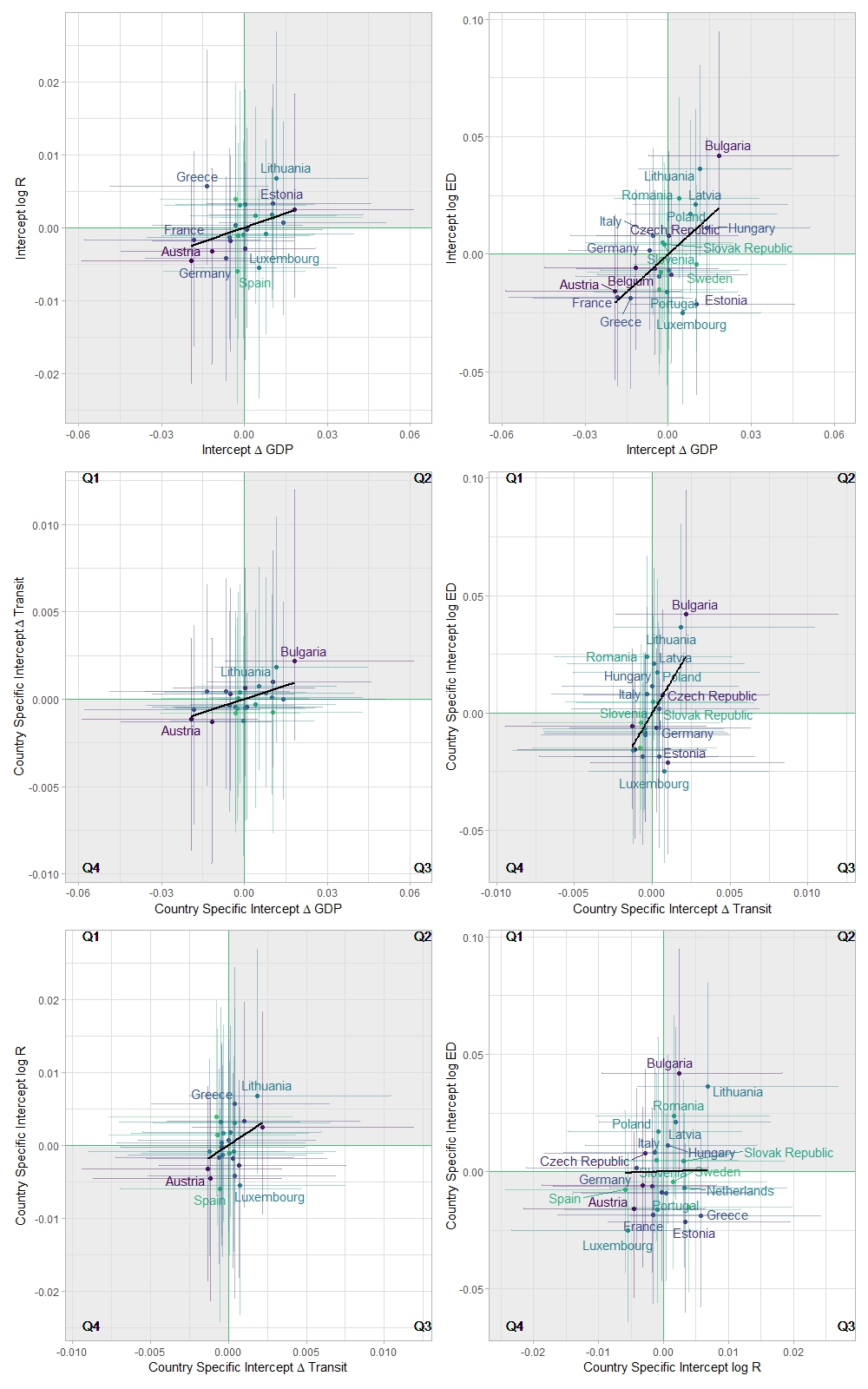
B.6 Principal Component Analysis of country specific characteristics
We can considering different types of clustering by constructing the principal components of the country characteristics, which we provide in Table S11. The correlation of the principal components is not significant with respect to any of the response variables, which is unsurprising as they are linear combinations of all covariates. We can consider how countries cluster together, either by considering k-means cluster in the plane of country specific intercepts against each other (left hand plot in Figure S19) or using a dimension reduction technique, here we use UMAP umap. The first & second UMAP components against each other are displayed in the right hand plot of Figure S19. In both cases we observe that we have clusters which correspond to regional areas in Europe and this is broadly consistent if we just consider country specific characteristics or country specific intercepts, in particular we see clusters around Eastern European countries.
| \topruleCovariate | Dim.1 | Dim.2 | Dim.3 | Dim.4 | Dim.5 |
| \midruleGovernment Effectiveness estimates, 2018 | 0.951 | -0.187 | 0.046 | -0.034 | -0.030 |
| Control of Corruption Index (WB, 2018) | 0.946 | -0.128 | 0.136 | 0.047 | -0.041 |
| Rule of Law (WB, 2018) | 0.918 | -0.217 | 0.154 | -0.006 | -0.057 |
| UN Human Development Index (WB, 2018) | 0.914 | 0.108 | 0.124 | -0.048 | 0.070 |
| RAND Infectious Disease Vulnerability Index | 0.914 | 0.088 | 0.037 | -0.087 | -0.011 |
| Financial institution account (% age 15+), 2017 | 0.894 | 0.116 | -0.115 | -0.186 | 0.118 |
| Used the internet to pay bills or to buy something online … | 0.893 | -0.013 | 0.170 | -0.051 | 0.048 |
| … in the past year (% age 15+), 2017 | |||||
| Property Rights (2018, Heritage Foundation) | 0.892 | -0.168 | 0.168 | -0.003 | 0.053 |
| Individuals using the Internet (% of population) | 0.867 | -0.133 | 0.231 | 0.048 | 0.064 |
| Used the internet to pay bills in the past year (% age 15+), 2017 | 0.865 | -0.190 | 0.175 | -0.039 | 0.056 |
| Proportion of Jobs That Are Teleworkable | 0.853 | 0.017 | -0.052 | 0.123 | 0.061 |
| Freedom House Global Freedom Score | 0.836 | -0.110 | -0.074 | -0.049 | 0.181 |
| Ratio of Female to Male Labor Force Participation (WB, 2018) | 0.808 | -0.405 | -0.009 | 0.056 | -0.023 |
| Regulation Freedom (2018, Heritage Foundation) | 0.761 | -0.231 | 0.053 | 0.048 | 0.190 |
| Health Expenditure as Fraction of GDP 2016 | 0.744 | 0.234 | 0.062 | 0.157 | -0.225 |
| Electric power consumption (kWh per capita), 2014 | 0.721 | -0.186 | -0.417 | 0.069 | -0.242 |
| Life Expectancy at Birth (WB, 2018) | 0.702 | 0.489 | -0.262 | -0.086 | 0.087 |
| Urban population (% of total population), 2018 | 0.632 | 0.188 | -0.121 | 0.679 | 0.032 |
| B40 share of income, 2020 | 0.491 | -0.013 | 0.251 | -0.428 | -0.368 |
| Number of Physicians per 100k population (2019, Eurostat) | 0.463 | 0.297 | -0.578 | -0.012 | -0.027 |
| Population density (people per sq. km of land area), 2018 | 0.357 | 0.577 | 0.459 | 0.381 | -0.152 |
| Proportion of Population Living Within 60 Minutes of an Urban Centre | 0.240 | 0.751 | 0.416 | -0.139 | -0.213 |
| Obedience | 0.028 | 0.502 | 0.174 | -0.387 | 0.343 |
| Labor Freedom (2018, Heritage Foundation) | -0.139 | -0.299 | 0.655 | 0.080 | 0.439 |
| Number of Hospital beds per 100k population (2019, Eurostat) | -0.549 | -0.135 | 0.286 | 0.086 | -0.628 |
| Extent and Prevalence of Labour Informality | -0.625 | 0.366 | 0.005 | 0.062 | 0.370 |
| Rural population (% of total population), 2017 | -0.632 | -0.188 | 0.121 | -0.679 | -0.032 |
| Infanty Mortality Per 1000 Live Births | -0.728 | -0.088 | 0.349 | 0.398 | -0.002 |
| Poverty Rate, 2020 | -0.820 | -0.165 | -0.043 | 0.336 | 0.108 |
B.7 Forecast comparison
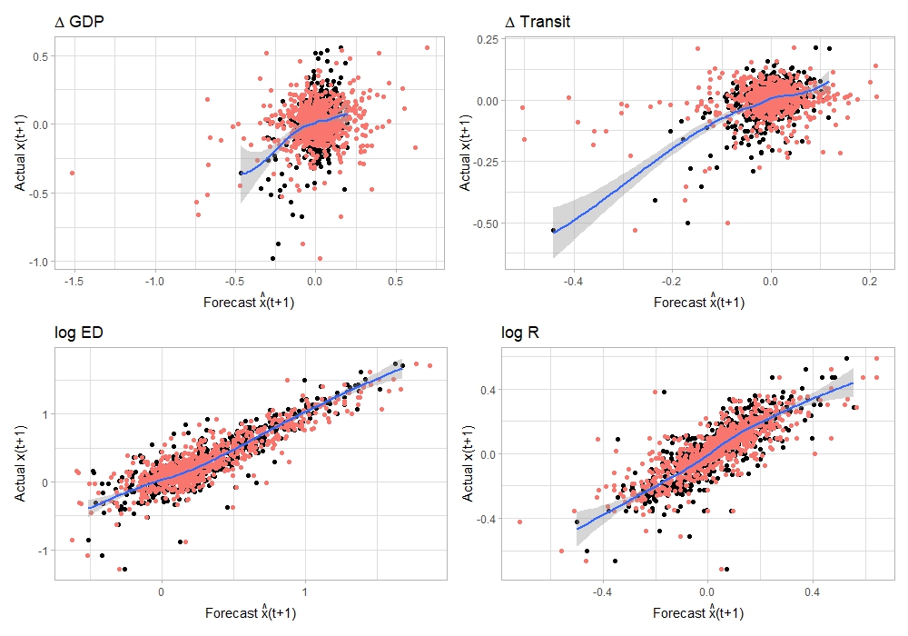
B.8 Convergence statistics
MCMC convergence statistics are available in Figure S21 and show the rank-normalized split score Vehtari2021-fx and relative Effective Sample Size MCMC convergence statistics. Values of close to 1 indicate convergence of the MCMC sampling algorithm. We note the sample properties are such for all estimated parameters Vehtari2021-fx (Figure S21). This implies that the posterior has converged and can be used for inference.
We used 2000 warmup samples and 2000 iterations per chain, for 4 chains. We also see that the relative effective sample size exceeds 0.5 for the majority of parameters, indicating low autocorrelation and fast mixing.
B.9 Sensitivity Analysis
In order to check that no single country overly influenced the estimation, we re-estimated the model 25 times, each time leaving out one of the countries in the analysis. In Figure S22, we plot the distribution of coefficients of the VAR component of the model. While there is some variation in the resulting coefficient estimates, this variation is generally small.
We also consider robustness for parameter choices in our model and estimation, such as . The variable selection broadly follows the approach taken in liu2021.
There are a range of different specification for the model. Rather than estimating the model with no intercept we could introduce a global intercept and impose a constraint on the wild type variant coefficient to equal zero. The estimated coefficients are essentially unchanged by this.
