Visualising Generative Spaces Using Convolutional Neural Network Embeddings
Abstract
As academic interest in procedural content generation (PCG) for games has increased, so has the need for methodologies for comparing and contrasting the output spaces of alternative PCG systems. In this paper we introduce and evaluate a novel approach for visualising the generative spaces of level generation systems, using embeddings extracted from a trained convolutional neural network. We evaluate the approach in terms of its ability to produce 2D visualisations of encoded game levels that correlate with their behavioural characteristics. The results across two alternative game domains, Super Mario and Boxoban, indicate that this approach is powerful in certain settings and that it has the potential to supersede alternative methods for visually comparing generative spaces. However its performance was also inconsistent across the domains investigated in this work, as well as it being susceptible to intermittent failure. We conclude that this method is worthy of further evaluation, but that future implementations of it would benefit from significant refinement.
Introduction
Procedural Content Generation (PCG) for games, despite being a relatively new research field, has become a very active and diverse one, with an increasing volume of novel works being produced across numerous subdomains of PCG research. Whenever a PCG system involves stochastic elements in its generative process to produce diverse output, it is important to understand what outputs are possible from a given system, a concept often referred to as a PCG system’s ‘generative space’. This is important for both PCG researchers, as well as game designers. In commercial settings, designers ideally want to know that all possible artefacts that could be generated from a given PCG system are desirable for their purposes, and that an alternative system or configuration would not produce better artefacts. Similarly, PCG researchers often want to be able to credibly claim that a novel system or approach is a meaningful improvement over what was previously possible, and the qualities of the output are a valuable component of any comparison.
In this work’s domain of PCG systems focused on the generation of game levels, a common approach for understanding generative spaces is to produce simplified visualisations of system output, most commonly using Expressive Range Analysis (ERA) [\citeauthoryearSmith and Whitehead2010]. ERA is an approach for understanding generative spaces by visualising a sample of levels in terms of two of their behavioural characteristics (BCs), which are most commonly heuristics for aesthetic or gameplay related qualities. ERA is commonly used for both the qualitative understanding of PCG system output, as well as quantitatively to compare aspects of alternative generators such as their relative diversities of output. However, ERA has several weaknesses as a visualisation approach, some of which we argue can be addressed with the alternative method presented in this paper. Most relevantly, ERA only allows for visualisions of generative spaces in terms of two BCs while maintaining the readability of a 2D graph, and also requires that BCs are calculated for every new set of levels to be visualised.
In this paper we present a novel alternative method for producing two dimensional visualisations of generative systems using Convolutional Neural Networks (CNNs), a subtype of deep learning system which are widely used for image recognition tasks [\citeauthoryearRussakovsky et al.2015]. The basic operation of this approach is as follows. First, we train a CNN to predict the BCs of levels based on their structure. This CNN is then used to extract embeddings for each level we wish to visualise from the penultimate layer of the network. These embeddings are assembled and then compressed using principal component analysis (PCA), a dimensionality reduction algorithm, to represent each level using only two dimensions. These compressions can then be visualised on a 2D scatter-plot in which each point represents a level. The goal is that these 2D visualisations are similar to conventional ERA, except that distance between levels is closely correlated with their values for multiple BC values rather than just two. The extent to which this is the case is the focus of this paper’s experiments. The stronger the correlation the more credibly we can claim that we are able to realise the benefits of ERA without some of its weaknesses.
Background and Related Work
Expressive Range Analysis
The most widely used and influential approach for visualising the generative spaces of PCG systems is Expressive Range Analysis (ERA). It was introduced by Gillian Smith and Jim Whitehead in 2010 [\citeauthoryearSmith and Whitehead2010] as a way for the designers of procedural level generators to understand their generative spaces.
Its basic mode of operation is appealingly simple. First a set of levels is generated to represent a generative space, and then annotated with BCs of interest (also often referred to as simply ‘metrics’ [\citeauthoryearHervé and Salge2021]). These BCs can be quantitative heuristics for aspects of the experience of playing a level, such as heuristics for difficulty [\citeauthoryearSmith and Whitehead2010, \citeauthoryearHorn et al.2014, \citeauthoryearJadhav and Guzdial2021], or they can be more abstract features such as how linear a level is [\citeauthoryearSmith and Whitehead2010]. The set of levels can then be visualised as a 2D scatter plot or heatmap, in which the levels location is specified by two selected BCs.
There have been some evolutions and innovations in how ERA can be applied, such as Summerville’s work on visualising multiple BCs simultaneously using corner plots [\citeauthoryearSummerville2018] and Cook et als work on designing interactive tools for conducting ERA on a PCG system with tunable parameters [\citeauthoryearCook et al.2021], but most commonly ERA is used in its original form and it is is still used in contemporary state-of-the-art PCG research [\citeauthoryearSmith, Padget, and Vidler2018, \citeauthoryearJadhav and Guzdial2021, \citeauthoryearAlvarez et al.2022].
Machine Learning and PCG
This work is also inspired by the domain of Machine Learning-based PCG approaches, commonly collectively referred to as PCGML. Over the past decade there has been a proliferation of different approaches using ML to tackle different challenges within PCG. They have been used to achieve diverse goals such as: generating new levels from single training examples [\citeauthoryearAwiszus, Schubert, and Rosenhahn2020]; blending training from alternative games to generate content for unseen games [\citeauthoryearJadhav and Guzdial2021]; and powering AI level design partners [\citeauthoryearGuzdial et al.2019]. A belief shared and reinforced by these works as well as this one, is that useful knowledge about game levels and their utility can be predicted from their representations using ML.
The approach in this paper uses a specific type of Neural Network called a Convolutional Neural Network (CNN). They are most commonly used for image recognition and analysis, but have also seen success in PCG research focused on level generation [\citeauthoryearWulff-Jensen et al.2018, \citeauthoryearVolz et al.2018, \citeauthoryearIrfan, Zafar, and Hassan2019]. However the primary inspiration for this approach did not come from the domain of PCG research but instead from that of art analysis, specifically the work of [\citeauthoryearGardini et al.2021]. They used a CNN-based approach to produce 2D visualisations of sets of artistic works which they then aimed to order based on age, without the system having prior knowledge of the creation date. Their use of CNNs to create information rich 2D representations of sets of artistic content appeared directly relevant to the challenge of visualising PCG generative spaces, and led to the development of this project.
In this work we make use of a popular CNN architecture called VGG-16 [\citeauthoryearSimonyan and Zisserman2015a], which was developed by Simonyan and Zisserman and was a winning entry in the ImageNet Large Scale Visual Recognition Challenge [\citeauthoryearRussakovsky et al.2015].
Level Generators and Benchmarks
In this work we make use of two open source level corpuses to experimentally assess our visualisation approach.
The Mario AI Benchmark is a widely used experimental platform which has helped to make Super Mario one of the most popular domains for both PCG research and game AI research more broadly. It was developed to support the 2009 Mario AI competition [\citeauthoryearTogelius, Karakovskiy, and Baumgarten2010] but it has gone on to be used in numerous research projects, including contemporary research on novel PCG approaches [\citeauthoryearAwiszus, Schubert, and Rosenhahn2020, \citeauthoryearFontaine et al.2021, \citeauthoryearSarkar, Yang, and Cooper2020, \citeauthoryearCerny Green et al.2020]. The modern version of the benchmark, supported by Ahmed Khalifa et al [\citeauthoryearKhalifa and Togelius2009], contains nine sets of 1000 Mario levels produced by different level generators as part of Horn et als work to compare alternative PCG systems [\citeauthoryearHorn et al.2014].
The other source of visualisable level sets that we make use of is Boxoban, an open source version of Sokoban developed by [\citeauthoryearGuez et al.2018] to support their research into model-free planning [\citeauthoryearGuez et al.2019]. As part of their work they released a large set of levels which were procedurally generated with the goal of having varying levels of challenge for reinforcement learning agents. It consists of over 1.5 million levels, each composed of a 10 by 10 grid with four goals. The levels are split into three sets: Medium, Hard and Unfiltered. The Medium and Hard sets were generated using the approach explained in [\citeauthoryearGuez et al.2019], and were sorted based on the ability of a trained agent to solve them. The Unfiltered set were generated using the approach of [\citeauthoryearRacanière et al.2017], implemented by Guez et al, and were not separated by difficulty.
Approach
In this section we present the main stages and steps involved in this approach for producing visualisations of sets of 2D game levels, as well as the process we used to investigate whether or not the visualisations contain useful information. The code used to create and validate the visualisations is available at github.com/KrellFace/Generative-Space-Compression.
Stage 1: CNN Architecture and Training
The first stage of the approach involves training a CNN to be able to predict level BCs based on the levels encoded structure. In this work we implement two alternative CNN architectures: VGG-16 and a simple 5 layer ‘Basic’ CNN to use as a comparison point for the larger and more complex VGG-16 implementation. In VGG-16’s original configuration, it used a softmax layer for its final layer to make class predictions for input images. However, as we are predicting BCs which are continuous numeric values we replace the softmax layer with a final dense layer. Apart from this change we use VGG-16 in its original configuration D form as described in [\citeauthoryearSimonyan and Zisserman2015b]. The simplified ‘Basic’ CNN we implement only uses three convolutional layers interlaced with two max pooling layers. See Table 1 for a more detailed description of the two architectures.
| Basic | VGG-16 |
|---|---|
| Conv-32 | Conv-64 x 2 |
| MaxPool | MaxPool |
| Conv-64 | Conv-128 x 2 |
| MaxPool | MaxPool |
| Conv-64 | Cov-256 x 3 |
| FC-64 | MaxPool |
| FC-(BC Count) | Conv-512 x 3 |
| MaxPool | |
| Conv-513 x 3 | |
| MaxPool | |
| FC-4096 x 2 | |
| FC-1000 | |
| FC-(BC Count) |
To allow the CNN to process the levels, we first convert their character based representations into one-hot encoded representations. In the Boxoban and Mario AI Benchmark level corpuses each level is stored as a two dimensional matrix of characters, in which each character represents a specific tile that appears at that position. We take these 2D representations and convert them into a three dimensional one-hot matrix, with the size of the 3rd dimension equal to the number of possible tile types. The 3D matrix is effectively an assembled set of 2D matrices for each tile type, in which each value is either 0, or 1 in the case that a tile of that matrix’s type appears at that location (See Figure 1 for a visual explanation). This conversion to one-hot matrices is often used in PCGML, and was directly inspired by the work of Volz et al on their work using GANs to generate Mario levels [\citeauthoryearVolz et al.2018].

For each training level, we first calculate its BCs and then process it into a one-hot 3D encoding. The CNN can then be trained to predict the BCs of unseen levels based on their one-hot encoded structures using this training data. Once training is completed the model is saved, ready for reuse in Stage 2.
Stage 2: Embedding Extraction and Compression
The next stage of the approach centres on using the trained neural network to produce level set visualisations in the form of 2D scatterplots, in which we intend that levels with similar BC values appear closer together in the visualisation than those with dissimilar characteristics.
To accomplish this we take every level to be visualised, which in this paper’s experiments are levels not used in the original training, and process them with an instance of the previously trained CNN. However, rather than using the predicted BC values, we instead extract the output features from the penultimate fully connected dense layer from the CNN instance. In the case of VGG-16 this means extracting a 1D feature map of size 1000, and for the ‘Basic’ CNN of size 64.
As we want to visualise these levels in two dimensional space, we then need to reduce the dimensionality of the data for each level. To achieve this we assemble the one dimensional feature maps for each level into a combined matrix, in which each row represents the penultimate layer outputs for a given level in the dataset to visualise. We then apply principal component analysis (PCA), a widely used dimensionality reduction algorithm to reduce the dimensionality of the dataset. PCA operates by constructing new variables out of linear combinations of the original variables in such a way that the top principal components account for the maximal possible variance in the data (See [\citeauthoryearAyesha, Hanif, and Talib2020] for a more detailed explanation of PCA). We can then select the top two principal components and use them to represent the sets of levels using two dimensions, while still accounting for a substantial amount of the variance found in the original N dimensions extracted from the CNN. These levels can then be visualised on a standard 2D scatter plot, with their positions dictated by the principal components.
Stage 3: Validating the Visualisations
The final stage of our approach is to validate whether the generated visualisations contain information that a human designer might find useful. In this work we use the same approach as [\citeauthoryearWithington and Tokarchuk2022] and look for correlation between euclidean distances between levels in the visualisations, and the difference between their BC values. If strong correlation is found between the euclidean distances and the BC differences, then that means that levels with similar values for the BCs are found close together, and those with dissimilar BC values are further apart.
To calculate the level of correlation we first calculate the euclidean distance between every level pair in the visualisation, as well as the absolute difference between their BC values. We then calculate Spearman’s rank correlation coefficient, also known as Spearman’s . Spearman’s is commonly used to investigate the linear correlation between variables when the distribution is not expected to be normal. It uses the relative rankings of the data points rather than their values, to give a coefficient score from 0 to 1 on how strong the correlation is, along with a P value indicating the likelihood that the correlation found is actually present. These correlation coefficients are then used as the heuristic for the performance of that visualisation. The expectation is that the stronger the correlation the more useful the visualisations would be to a designer.

Experiment Design
In this section we explain the design of the experiments that we ran to conduct an initial investigation of this approach.
Level Sets and Encodings
For these experiments we use two pre-generated level corpuses: the level sets provided as part of the Mario AI Benchmark and the training levels provided as part of Guez et als research using Boxoban. Both corpuses meet several requirements for a straightforward application of the approach we present in this work. Both are composed of 2D tile-based levels in which every tile type is represented by one of a discrete set of values. Each level also has the same fixed size, 10 x 10 in the case of Boxoban and 16 x 100 in the case of the Mario AI Benchmark, which avoids the need to regularise them before training the CNN.
The two sets are also interestingly distinct. The Mario level sets come from a set of nine distinct generators with substantial variety in their structural and gameplay features (See both [\citeauthoryearHorn et al.2014] and [\citeauthoryearWithington and Tokarchuk2022] for evidence of this). In contrast the Boxoban set all come from similar generative approaches implemented by the same team and are differentiated instead by difficulty, a trait that is less obvious than structural features. This combined with the smaller level representations, and the commonalities between all levels (all containing four boxes and four goals) mean it is significantly harder to differentiate between different levels. It is hoped that the difference of these two sets will help to highlight different strengths and weaknesses of the tested visualisation approaches.
In terms of the encoding used, in the case of Boxoban no preprocessing was required. Only five tile types are used in the level representation (empty, solid, box, goal, player) and we use all five in the one-hot encodings, giving a one-hot matrix with dimensions (10, 10, 5). In the case of the Mario level sets we conduct a preprocessing step of condensing the original tile types into a smaller grouped set. The original representations are composed of 28 total tile types, each of which we map to one of five values. All traversable tiles (including tiles that indicate the spawn point and level end point) are mapped to empty space and all enemies are mapped to a unifying enemy type. The same is done with solid blocks, pipe blocks and blocks that contain a reward. While this reduces the accuracy of the representations, it does increase the performance by reducing the complexity. The one hot representations are therefore of size (10, 16, 5).
Behavioural Characteristics Used
For both Mario and Boxoban domains we calculate four BCs for each level. Each BC is either one directly used in or inspired by prior work using ERA or Quality-Diversity (QD)-based PCG. QD-based PCG requires a designer to determine at least two behavioural dimensions to define the diversity component of the search, making it a valuable source of inspiration for BCs. Each BC was selected for both being fast to calculate from the level representation, as well as appearing in prior PCG work.
The four BCs calculated for the Mario domain were as follows: Empty Space (ES), a simple count of empty tiles, which was inspired by ERA implementations such as [\citeauthoryearJemmali et al.2020] which use block count-based BCs as quick to calculate heuristics for diversity. ES was calculated for both the Mario and Boxoban domains. Enemy Count (EC), Linearity (Lin) and Density (Dens) are all BCs which have been widely used in ERA applied to procedurally generated platformer levels [\citeauthoryearSmith and Whitehead2010, \citeauthoryearHorn et al.2014, \citeauthoryearJadhav and Guzdial2021], and make up the remaining three BCs calculated for the Mario levels.
ERA and QD-search has been less commonly applied to top-down games like Boxoban than to platformer games like Super Mario. However, there are still sources to draw on. We calculate the Contiguity Score (CS), a BC which has been used in prior QD-search based PCG [\citeauthoryearWithington2020], which measures how clustered together the solid tiles in a level are by incrementing the score by 1 for every solid block that is adjacent to another. We also calculate the Adjusted Contiguity Score (ACS), which divides the CS by the number of solid blocks present to give a heuristic for tile clustering independent of their number. Finally we calculate a Corridor Count (CC), which counts every location in the level in which the player can only move north or south but not east or west, or vice versa. This is intended to be a similar BC to Density except applicable to a top down game, and has appeared in work such as [\citeauthoryearAlvarez et al.2022].
Compression Approaches Used
As discussed in more detail in the Approach section, we implement two alternative CNN architectures to produce alternative visualisations, referred to in results as ‘VGG-16’ and ‘Basic’.
We also implement the approach of [\citeauthoryearWithington and Tokarchuk2022], which works similarly to this paper’s CNN based approach except without the CNN processing layer. Instead of using PCA to compress the CNN embeddings, PCA is instead applied directly to the one-hot encoded levels. This approach makes for an interesting benchmark, as it both aims to generate similar 2D visualisations of generative spaces, while also requiring less setup and configuration in the form of calculating BCs and model training. We refer to this as ‘Vanilla DR’ in these experiments.
In this work we do not report on the explained variance of the top two principal components derived from applying PCA within any of the approaches as it is not relevant to the quality final output. However, prior reviews of this work have highlighted that explained variance could be a valuable metric to extract during CNN training for evaluating how effectively the model is learning to indirectly produce the desired visualisation, something we aim to investigate in future work.
CNN Parameters
Both networks were compiled with an Adam optimizer. After initial experimentation a learning rate of 0.01 was selected for the basic CNN, and 0.0005 for VGG-16, as this appeared to give the best performance in their respective architectures. Both used the mean absolute error (MAE) for their loss functions. MAE was selected as the loss function as we expected there to be significant level outliers in terms of their BC values, a feature better accounted for by calculating absolute errors rather than an average.
Each CNN instance was given 100 epochs in which to train, though in the final experiments there were minimal improvements in terms of loss from as early as epoch 30 in certain configurations. Future implementations could usefully implement early stopping to avoid over-fitting and to save on computational resources.
Level Selection and Splitting
For each run 1000 levels were selected at random, distributed evenly between each generative approach for each game. For Mario they were evenly selected from the nine different generators, and for Boxoban they were evenly split between the three different sets.
For each combination of BC and CNN design a new instance of the network was generated and trained. For the CNN training, the 1000 levels were split into a set of 800 used to train the network, and a set of 200 to produce the final visualisation.
We note that we are using a comparatively low amount of data to both train and test the neural networks. With just 1000 levels per run, a train/test split of 0.8 and a high of nine generators for the Mario domain this means that there are less than 90 levels from each generator in each training set. While this choice was primarily made to limit the computational resources required, it also helps to reinforce any potential claim about this approach having commercial utility. The more data that is required for a given generative space visualisation approach, the less widely useful it can be in domains where generating levels is either resource intensive, or in domains where it is a requirement to test numerous different configurations of a generator.
Number of Runs
To increase the reliability of the results and to gain insight into how much variance there is with the approach, we conduct five runs for each of the two games and then present the average of the results for each compression method.
Resources Required
All experiments were run on a Dell laptop with an i5-10310U CPU with 16.0 GB of RAM. In total all experiments took 11 hours to run using this set up.
Results & Discussion
| Mario | Boxoban | |||||||||||||||||||||||
|---|---|---|---|---|---|---|---|---|---|---|---|---|---|---|---|---|---|---|---|---|---|---|---|---|
| ES | EC | Lin | Dens | ES | CS | ACS | CC | |||||||||||||||||
| VGG-16 |
|
|
|
|
|
|
|
| ||||||||||||||||
| CNN-Basic |
|
|
|
|
|
|
|
| ||||||||||||||||
| Vanilla DR |
|
|
|
|
|
|
|
| ||||||||||||||||

Results Overview
The experimental results give us a view of our approach that is both positive overall, but also mixed. The CNN-based visualisations substantially outperformed Vanilla DR in the Boxoban domain in terms of the BC correlations of their visualisations, and also performed well on individual BCs in the Mario domain. However, there was significant inconsistency in the performance of CNN approaches, suggesting that while the approach is promising, the implementation used needs significant refinement.
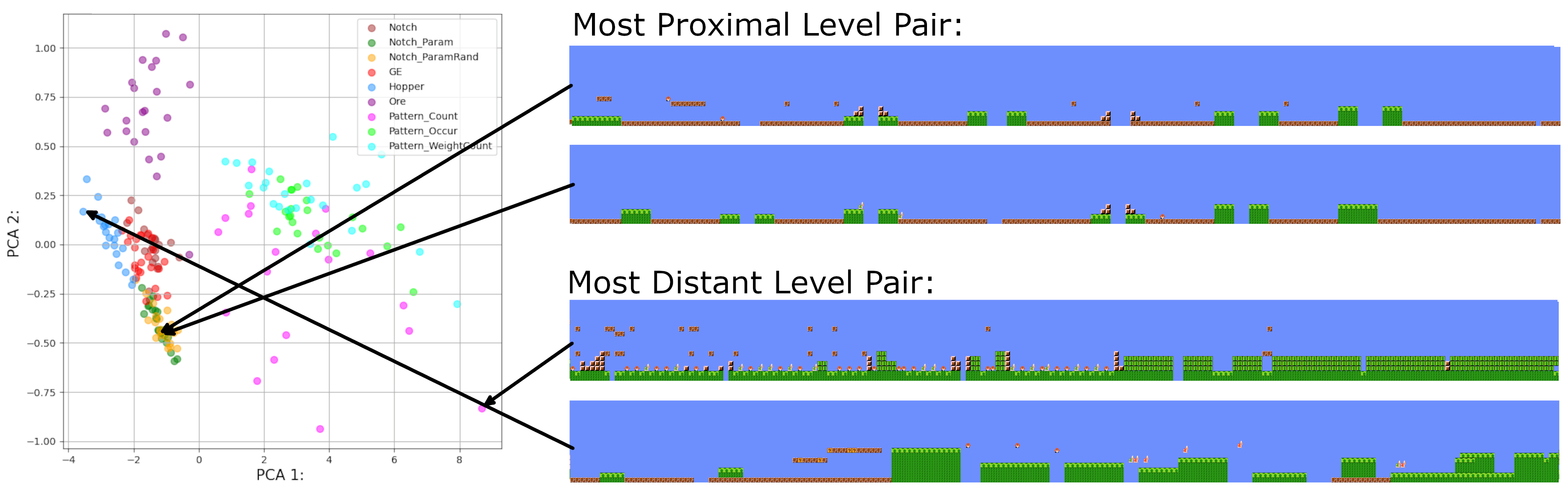
In Figures 3 and 4 show the best performing visualisations in terms of average BC correlation for the Boxoban and Mario domains respectively. These are presented to demonstrate what the final output of the visualisation process is, as well as to give an idea of how it could be used to qualitatively understand and compare generators. For example, the Mario visualisation suggests that the Ore generator highlighted in dark purple generates levels unlike any alternatives, whereas the Boxoban visualisation suggests that none of the three generative approaches produces substantially different levels to the other two. The fact that at least in the Mario domain the visualisation approach was able to separate and distinguish between the levels from alternative generators is positive, as characterising the output of alternative generators is a valuable potential use case.
Displayed with each visualisation is the pairs of levels which are the most proximal and distant in terms of their Euclidean distance in the visualisation. If the visualisation is working well, we would expect the most proximal pair to be the most similar pair of levels in the set and visa versa. They suggest that while the Boxoban visualisations performed better than those for Mario in terms of the BC correlation heuristics, that this may not mean the visualisations are in fact more useful. If we examine the most proximal pair in Figure 3, it is not obvious that the levels are especially similar or that the experience of playing them would be similar either. In contrast the most proximal Mario pair in Figure 4 do appear substantially similar. It is possible that the smaller a game level’s representation is, the more important each tile choice becomes, and therefore the more important attaining a high level of BC correlation becomes.
We expected due to its complexity and performance in other domains, that VGG-16 would outperform both the basic CNN and the Vanilla DR visualisations, and in 4/8 domains this was the case as we can see in Table 2. Its performance was dominant in visualising the Boxoban domains, only struggling on the CC BC. However, given the underperformance across the board on the CC BC, we expect this to be an issue related to the structure of the CNN’s themselves, perhaps related to the convolutional window being too small to detect the corridor structure. The Basic CNN implementation also substantially outperformed Vanilla DR in the Boxoban domain, further reinforcing the idea that this CNN-based approach can perform well for certain games.
However, in the Mario domain the results were much more mixed. VGG-16 performed worse than the simple Basic CNN in 3 of 4 BCs, and Basic CNN was outperformed by Vanilla DR in 2 of 4. We suspect this failure is partly a result of quirks of the dataset. Vanilla DR found average EC correlations of 0.337, despite enemies being a sparse feature in most levels which should mean Vanilla DR is worse at accounting for them. This leads us to suspect that within the levels tested, EC correlates significantly with the easier to detect structural features like the amount of empty space. The poor performance of the CNN-based approaches is still concerning however, especially as they require significantly more set-up and compute costs than Vanilla DR.
Additionally, the CNN-based approaches were prone to failure. Despite performing best in the Boxoban domain, the standard deviations for VGG-16 correlations were as high as 0.303 in the case of the ES BC. Examining the individual run data for both it and the Basic CNN shows that in some runs each CNN implementation failed during training to learn the relationship between level structure and BCs. Further experimentation is needed to investigate what was causing the intermittent failures, something we discuss in the next section.
Future Work and Improvements
On the technical front the primary aspect we need to address is the performance of the CNN training process. While we cannot be certain of what was causing the intermittent failures we have several different options to explore. First, we intend to further investigate the effect of tuning hyperparameters such as the learning rate to achieve a more consistent performance. We can also implement and evaluate alternative CNN implementations which have outperformed VGG-16 in certain domains, such as ResNet-50 [\citeauthoryearHe et al.2016] and Xception [\citeauthoryearChollet2017]. However, all of these architectures share the conceptual weakness in that they were designed and optimised for analysing images rather than encoded game levels. Future work could investigate whether a bespoke CNN architecture for predicting level BCs could give improved results.
Our future work will also further explore the performance gap between the Mario and Boxoban domains. It is possible that Vanilla DR is simply especially well suited to these specific Mario level sets, or that the CNN visualisation approach is ill suited to the larger level representations. Beyond further tuning the CNN training parameters, the best way of exploring this discrepancy is to explore alternative generative spaces, defined by alternative BCs. Related to this point, we also intend to start including BCs extracted from simulated play of the input levels by a level playing agent. If this approach produces correlations with these more complex BCs, this would be a cause for further optimism.
To make this approach more widely useful and accessible to game designers and researchers, we aim to investigate making the visualisation system publicly available in a form that could be quickly applied to new generators and new game domains. This could take the form of pre-trained CNNs embedded within a system that could be deployed to allow designers and researchers to produce visualisations without the need for training. It would also benefit from the development of an analytics layer, such as systems for displaying images of the outliers within a given generative space, or for giving representative samples of levels that are present within one generative space but not another.
Conclusion
In this paper we introduced a novel approach for producing visualisations of the generative spaces of 2D level generators using trained CNNs, and conducted preliminary experiments using the approach on two level corpuses from Super Mario and Boxoban. The results indicated that it had the capacity to produce relatively robust results, but also that the current implementation is significantly prone to failure, as well as it under-performing compared to our benchmark visualisation approach in certain domains. As a result we find that while this approach has promise and warrants further investigation, more experimentation and tuning is required before it can be used reliably.
Acknowledgements
This work was supported by the EPSRC Centre for Doctoral Training in Intelligent Games & Games Intelligence (IGGI) [EP/S022325/1]. We are also grateful for the helpful and informative feedback we received from the EXAG reviewers on the initial version of this work.
References
- [\citeauthoryearAlvarez et al.2022] Alvarez, A.; Dahlskog, S.; Font, J.; and Togelius, J. 2022. Interactive Constrained MAP-Elites: Analysis and Evaluation of the Expressiveness of the Feature Dimensions. IEEE Transactions on Games 14(2):202–211.
- [\citeauthoryearAwiszus, Schubert, and Rosenhahn2020] Awiszus, M.; Schubert, F.; and Rosenhahn, B. 2020. TOAD-GAN: Coherent style level generation from a single example. In Proceedings of the sixteenth AAAI conference on artificial intelligence and interactive digital entertainment, AIIDE’20. AAAI Press. Number of pages: 7 tex.articleno: 2.
- [\citeauthoryearAyesha, Hanif, and Talib2020] Ayesha, S.; Hanif, M. K.; and Talib, R. 2020. Overview and comparative study of dimensionality reduction techniques for high dimensional data. Information Fusion 59(Information Fusion):44–58.
- [\citeauthoryearCerny Green et al.2020] Cerny Green, M.; Mugrai, L.; Khalifa, A.; and Togelius, J. 2020. Mario Level Generation From Mechanics Using Scene Stitching. In 2020 IEEE Conference on Games (CoG), 49–56. Osaka, Japan: IEEE.
- [\citeauthoryearChollet2017] Chollet, F. 2017. Xception: Deep Learning with Depthwise Separable Convolutions. In 2017 IEEE Conference on Computer Vision and Pattern Recognition (CVPR), 1800–1807. Honolulu, HI: IEEE.
- [\citeauthoryearCook et al.2021] Cook, M.; Gow, J.; Smith, G.; and Colton, S. 2021. Danesh: Interactive Tools For Understanding Procedural Content Generators. IEEE Transactions on Games.
- [\citeauthoryearFontaine et al.2021] Fontaine, M. C.; Liu, R.; Khalifa, A.; Togelius, J.; Hoover, A. K.; and Nikolaidis, S. 2021. Illuminating Mario Scenes in the Latent Space of a Generative Adversarial Network. In AAAI.
- [\citeauthoryearGardini et al.2021] Gardini, E.; Ferrarotti, M. J.; Cavalli, A.; and Decherchi, S. 2021. Using Principal Paths to Walk Through Music and Visual Art Style Spaces Induced by Convolutional Neural Networks. Cognitive Computation 13(2):570–582.
- [\citeauthoryearGuez et al.2018] Guez, A.; Mehdi, M.; Gregor, K.; Kabra, R.; Racaniere, S.; Weber, T.; Raposo, D.; Santoro, A.; Orseau, L.; Eccles, T.; Wayne, G.; Silver, D.; and Lillicrap, T. 2018. An investigation of Model-free planning: boxoban levels.
- [\citeauthoryearGuez et al.2019] Guez, A.; Mirza, M.; Gregor, K.; Kabra, R.; Racanière, S.; Weber, T.; Raposo, D.; Santoro, A.; Orseau, L.; Eccles, T.; and others. 2019. An investigation of model-free planning. In International Conference on Machine Learning, 2464–2473. PMLR.
- [\citeauthoryearGuzdial et al.2019] Guzdial, M.; Liao, N.; Chen, J.; Chen, S.-Y.; Shah, S.; Shah, V.; Reno, J.; Smith, G.; and Riedl, M. O. 2019. Friend, Collaborator, Student, Manager: How Design of an AI-Driven Game Level Editor Affects Creators. In Proceedings of the 2019 CHI Conference on Human Factors in Computing Systems, 1–13. Glasgow Scotland Uk: ACM.
- [\citeauthoryearHe et al.2016] He, K.; Zhang, X.; Ren, S.; and Sun, J. 2016. Deep Residual Learning for Image Recognition. In 2016 IEEE Conference on Computer Vision and Pattern Recognition (CVPR), 770–778. Las Vegas, NV, USA: IEEE.
- [\citeauthoryearHervé and Salge2021] Hervé, J.-B., and Salge, C. 2021. Comparing PCG Metrics with Human Evaluation in Minecraft Settlement Generation. In The 16th International Conference on the Foundations of Digital Games (FDG) 2021, FDG’21. New York, NY, USA: Association for Computing Machinery. event-place: Montreal, QC, Canada.
- [\citeauthoryearHorn et al.2014] Horn, B.; Dahlskog, S.; Shaker, N.; Smith, G.; and Togelius, J. 2014. A comparative evaluation of procedural level generators in the Mario AI framework. In Mateas, M.; Barnes, T.; and Bogost, I., eds., Proceedings of the 9th International Conference on the Foundations of Digital Games, FDG 2014, Liberty of the Seas, Caribbean, April 3-7, 2014. Society for the Advancement of the Science of Digital Games.
- [\citeauthoryearIrfan, Zafar, and Hassan2019] Irfan, A.; Zafar, A.; and Hassan, S. 2019. Evolving Levels for General Games Using Deep Convolutional Generative Adversarial Networks. In 2019 11th Computer Science and Electronic Engineering (CEEC), 96–101. Colchester, United Kingdom: IEEE.
- [\citeauthoryearJadhav and Guzdial2021] Jadhav, M., and Guzdial, M. 2021. Tile embedding: A general representation for level generation. Proceedings of the AAAI Conference on Artificial Intelligence and Interactive Digital Entertainment 17(1):34–41.
- [\citeauthoryearJemmali et al.2020] Jemmali, C.; Ithier, C.; Cooper, S.; and El-Nasr, M. 2020. Grammar based modular level generator for a programming puzzle game. AAAI Conference on Artificial Intelligence and Interactive Digital Entertainment (AIIDE).
- [\citeauthoryearKhalifa and Togelius2009] Khalifa, A., and Togelius, J. 2009. Mario AI Benchmark - https://github.com/amidos2006/Mario-AI-Framework.
- [\citeauthoryearRacanière et al.2017] Racanière, S.; Weber, T.; Reichert, D. P.; Buesing, L.; Guez, A.; Rezende, D.; Badia, A. P.; Vinyals, O.; Heess, N.; Li, Y.; Pascanu, R.; Battaglia, P.; Hassabis, D.; Silver, D.; and Wierstra, D. 2017. Imagination-Augmented Agents for Deep Reinforcement Learning. In Proceedings of the 31st International Conference on Neural Information Processing Systems, NIPS’17, 5694–5705. Red Hook, NY, USA: Curran Associates Inc. event-place: Long Beach, California, USA.
- [\citeauthoryearRussakovsky et al.2015] Russakovsky, O.; Deng, J.; Su, H.; Krause, J.; Satheesh, S.; Ma, S.; Huang, Z.; Karpathy, A.; Khosla, A.; Bernstein, M.; Berg, A. C.; and Fei-Fei, L. 2015. ImageNet Large Scale Visual Recognition Challenge. International Journal of Computer Vision 115(3):211–252.
- [\citeauthoryearSarkar, Yang, and Cooper2020] Sarkar, A.; Yang, Z.; and Cooper, S. 2020. Controllable Level Blending between Games using Variational Autoencoders. arXiv:2002.11869 [cs]. arXiv: 2002.11869.
- [\citeauthoryearSimonyan and Zisserman2015a] Simonyan, K., and Zisserman, A. 2015a. Very deep convolutional networks for large-scale image recognition. CoRR abs/1409.1556.
- [\citeauthoryearSimonyan and Zisserman2015b] Simonyan, K., and Zisserman, A. 2015b. Very Deep Convolutional Networks for Large-Scale Image Recognition. arXiv:1409.1556 [cs].
- [\citeauthoryearSmith and Whitehead2010] Smith, G., and Whitehead, J. 2010. Analyzing the expressive range of a level generator. In Proceedings of the 2010 Workshop on Procedural Content Generation in Games - PCGames ’10, 1–7. Monterey, California: ACM Press.
- [\citeauthoryearSmith, Padget, and Vidler2018] Smith, T.; Padget, J.; and Vidler, A. 2018. Graph-based generation of action-adventure dungeon levels using answer set programming. In Proceedings of the 13th International Conference on the Foundations of Digital Games, 1–10. Malmö Sweden: ACM.
- [\citeauthoryearSummerville2018] Summerville, A. 2018. Expanding Expressive Range: Evaluation Methodologies for Procedural Content Generation. In Fourteenth Artificial Intelligence and Interactive Digital Entertainment Conference.
- [\citeauthoryearTogelius, Karakovskiy, and Baumgarten2010] Togelius, J.; Karakovskiy, S.; and Baumgarten, R. 2010. The 2009 Mario AI Competition. In IEEE Congress on Evolutionary Computation, 1–8. Barcelona, Spain: IEEE.
- [\citeauthoryearVolz et al.2018] Volz, V.; Schrum, J.; Liu, J.; Lucas, S. M.; Smith, A.; and Risi, S. 2018. Evolving mario levels in the latent space of a deep convolutional generative adversarial network. In Proceedings of the Genetic and Evolutionary Computation Conference, 221–228. Kyoto Japan: ACM.
- [\citeauthoryearWithington and Tokarchuk2022] Withington, O., and Tokarchuk, L. 2022. Compressing and Comparing the Generative Spaces of Procedural Content Generators. arXiv:2205.15133 [cs].
- [\citeauthoryearWithington2020] Withington, O. 2020. Illuminating super mario bros: quality-diversity within platformer level generation. In Proceedings of the 2020 Genetic and Evolutionary Computation Conference Companion, 223–224. Cancún Mexico: ACM.
- [\citeauthoryearWulff-Jensen et al.2018] Wulff-Jensen, A.; Rant, N. N.; Møller, T. N.; and Billeskov, J. A. 2018. Deep Convolutional Generative Adversarial Network for Procedural 3D Landscape Generation Based on DEM. In Brooks, A. L.; Brooks, E.; and Vidakis, N., eds., Interactivity, Game Creation, Design, Learning, and Innovation, volume 229. Cham: Springer International Publishing. 85–94. Series Title: Lecture Notes of the Institute for Computer Sciences, Social Informatics and Telecommunications Engineering.