Diffusion-based Generative Speech Source Separation
Abstract
We propose DiffSep, a new single channel source separation method based on score-matching of a stochastic differential equation (SDE). We craft a tailored continuous time diffusion-mixing process starting from the separated sources and converging to a Gaussian distribution centered on their mixture. This formulation lets us apply the machinery of score-based generative modelling. First, we train a neural network to approximate the score function of the marginal probabilities or the diffusion-mixing process. Then, we use it to solve the reverse time SDE that progressively separates the sources starting from their mixture. We propose a modified training strategy to handle model mismatch and source permutation ambiguity. Experiments on the WSJ0_2mix dataset demonstrate the potential of the method. Furthermore, the method is also suitable for speech enhancement and shows performance competitive with prior work on the VoiceBank-DEMAND dataset.
Index Terms:
source separation, stochastic differential equation, diffusion, score matching1 Introduction
Source separation (SS) refers to a family of techniques that can be used to recover signals of interests from their mixtures. It has broad applications, but we focus on single channel audio and speech [1]. This is an underdetermined problem where several signals are recovered from a single mixture. Early success in this area was made with methods such as non-negative matrix factorization (NMF) [2]. Impressive progress was brought by data-driven methods and deep neural networks (DNN). We mention deep clustering where a DNN is trained to create an embedding space in which the time-frequency bins of the input spectrogram cluster by source [3]. Then, one can recover isolated sources by creating masks corresponding to clusters of bins and multiply the spectrogram with it. These methods then evolved to networks predicting mask values directly [4]. All these data-driven methods require to solve the fundamental source permutation ambiguity. Namely, there is no inherent preferred order for the sources. This is usually handled by permutation invariant training (PIT) [5]. In PIT, the objective function is computed for all permutations of the sources and the one with minimum value is chosen to compute the gradient. Recently very strong time-domain baselines such as Conv-TasNet [6] or dual-path transformer [7] have been proposed. We mention also all-attention based [8], multi-scale networks [9], WaveSplit [10], and the recent state-of-the-art TF-GridNet [11] back in the time-frequency domain. For a survey and benchmarks of recent methods see [12, 11]. All these recent approaches are trained with a discriminative objective such as the scale-invariant signal-to-distortion ratio (SI-SDR) [13]. Except the traditional methods, such as NMF, few approaches leverage generative models. One exception adversarially trains speaker-specific generative models and uses them for separation [14].
Unlike discriminative methods, generative modelling allows to approximate complex data distributions [15]. Recently, score-based generative modelling (SGM) [16], also known as diffusion-based modelling, has made rapid and impressive progress, in particular in the domain of image generation [17]. SGM defines a forward process that progressively transforms a sample of the target distribution into Gaussian noise. Given its score-function, i.e., the gradient of the log-probability, the target distribution can be sampled by running a reverse process starting from noise. Crucially, the score-function is (usually) unknown, but can be approximated by a DNN using a simple training strategy [18]. Recent approaches result from the combination of score-matching and Langevin sampling [16, 19, 20]. Two frameworks have been proposed to unify various approaches, one based on graphical models [21], and the other on stochastic differential equations (SDE) [22]. SGM has quickly found application in audio and speech processing. It has been successfully applied in speech synthesis [23, 24, 25, 26], speech restoration [27, 28], and bandwidth extension [29]. Surprisingly, perhaps, several SGMs have been proposed for speech enhancement, a typically discriminative task [30, 31, 32, 33]. Besides sound, but perhaps closest to this work, separation of images using deep generative priors and Langevin sampling has been demonstrated [34]. However, to the best of our knowledge, a diffusion-based speech separation method has yet to be proposed.
We fill this gap by proposing what we believe is the first diffusion-based approach for the separation of speech signals. The proposed algorithm, DiffSep, is based on a carefully designed SDE that starts from the separated signals and converges in average to their mixture. Then, by solving the corresponding reverse-time SDE, it is possible to recover the individual sources from their mixture. See Fig. 1 for an illustration. We propose a modified training strategy for the score-matching network that addresses ambiguity in the assignment of the sources at the beginning of the inference process. We demonstrate the method on the widely used WSJ0_2mix benchmark dataset [3]. While it does not outperform, yet, discriminative baselines in terms of separation metrics, it achieves high non-intrusive DNSMOS P.835 [35] score, indicating naturalness. In addition, our approach is also suitable for speech enhancement by considering the noise as just an extra source, and performs comparably to prior work [32] on the VoiceBank-DEMAND dataset [36].
2 Background
2.1 Notation and Signal Model
Vectors and matrices are represented by bold lower and upper case letters, respectively. The norm of vector is written . The identity matrix is denoted by .
We represent audio signals with samples by real valued vectors from . We introduce a simple mixture model with sources,
| (1) |
where for all . We remark that this model can account for environmental noise, reverberation, and other degradation by adding an extra source. By concatenating all the source signals, we obtain vectors in . We define in this notation the vector of separated sources and their average value,
| (2) |
We can define the time-invariant mixing operation as a multiplication by where is a matrix, and is the Kronecker product. Multiplying a vector by such a matrix amounts to multiplying by all sub-vectors of length with elements taken from at interval , i.e.,
To lighten the notation, we overload the regular matrix product as in the rest of this paper. Next, we define the projection matrices
| (5) |
where is the all one vector, of size here. The matrix projects onto the subspace of average values, and its orthogonal complement. For example, a compact alternative to (1) is .
2.2 SDE for Score-based Generative Modelling
Score-based generative modelling (SGM) via SDE is a principled approach to model complex data distributions [22]. First, a diffusion process starting from samples from the target distribution and converging to a Gaussian distribution can be described by the following stochastic differential equation
| (6) |
where is a vector-valued function of the time , is its derivative with respect to , and an infinitesimal time step. Functions and are called the drift and diffusion coefficients of . The term is a standard Wiener process. For more details on SDEs, see [37]. We insist that the time in the diffusion process is unrelated to the time of the audio signals that will appear later in this paper.
A remarkable property of (6) is that under some mild conditions, there exists a corresponding reverse-time SDE,
| (7) |
going from to [38]. Here, is a reverse Brownian process, and is the marginal distribution of .
During the forward process, being known, it is usually possible to have a closed-form formula for . For an affine , it is Gaussian and its parameters, i.e., mean and covariance matrix, usually tractable [37]. However, in the reverse process, is unknown, and thus (7) cannot be solved directly. The key idea of SGM [16, 19, 22] is to train a neural network so that . Provided that the approximation is good enough, we can generate samples from the distribution of by numerically solving (7), replacing by .
2.3 Related Work in Diffusion-based Speech Processing
SGM first found widespread adoption for the generation of very high quality synthetic images, e.g. [17]. Speech synthesis is thus a logical candidate for its adoption [23, 24]. In this area, several approaches that shape the noise adaptively for the target speech have been proposed. One uses the local signal energy [25], while the other introduces correlation in the noise according to the target spectrogram [26]. Bandwidth extension and restoration also require to generate missing parts of the audio and high quality diffusion-based approaches have been proposed [29, 27, 28]. Diffuse [30] and CDiffuse [31] use conditional probabilistic diffusion to enhance a noisy speech signal. Also for speech enhancement, Richter et al. have proposed another approach [32, 33] based on solving the reverse-time SDE corresponding to the forward model
| (8) |
This is the Ornstein-Uhlenbeck SDE that, in the forward direction, takes the clean speech progressively towards the noisy one .
3 Diffusion-based Source Separation
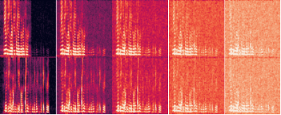
We propose a framework for applying SGM to the source separation problem. Essentially, we design a forward SDE where both diffusion and mixing across sources happen over time. Each step of the process can be described as adding an infinitesimal amount of noise and doing an infinitesimal amount of mixing. This can be formalized as the following SDE
| (9) |
where is defined in (5) and in (2). We use the diffusion coefficient of the Variance Exploding SDE of Song et al. [22],
| (10) |
The SDE (9) has the interesting property that the mean of the marginal goes from the vector of separated signals at to the mixture vector as grows large. This is formalized in the following theorem proved in Appendix 6.
Theorem 1.
The marginal distribution of is Gaussian with mean and covariance matrix
| (11) | ||||
| (12) |
where if we let , , and , then,
| (13) |
Fig. 1 shows an example of the process on a real mixture. We now have an explicit expression for a sample ,
| (14) |
where . Fig. 2 shows the evolution of some of the parameters of the distribution of over time. We can make the difference of and arbitrarily small by tuning the value of . In addition, we observe that the correlation of the noise added onto both sources increases over time due to the mixing process.
Previous work on speech enhancement has successfully applied the diffusion process in the short-time Fourier transform (STFT) domain with a non-linear transform [33, 32]. The approach we propose could be equally applied in the time-domain or in any linearly transformed domain such as the STFT. However, since the process of (9) models the linear mixing of the sources, we cannot apply a non-linear transformation. Instead, we perform the diffusion process in the time-domain, but operate our network in the non-linear STFT domain of [33], as described in Section 4.2.
3.1 Inference
At inference time, the separation is done by solving (7) with the help of a score-matching network . The initial value of the process is sampled from the distribution,
| (15) |
Then, we adopt the predictor-corrector approach described in [22] to solve (7). The prediction step is done by reverse diffuse sampling. The correction is done by annealed Langevin sampling [20].
3.2 Permutation and Mismatch-aware Training Procedure
To train the score network , we propose a slightly modified score-matching procedure. But, first, we follow the usual procedure. Thanks to Theorem 1, the score function has a closed form expression. The computation is similar to that in [32], and we obtain
| (16) |
The training loss is
| (17) | ||||
| (18) |
where , , and is chosen at random from the dataset. We use the norm induced by which is equivalent to the weighting scheme proposed by Song et al. [16]. This scheme makes the order of magnitude of the cost independent of and lets us avoid the computation of the inverse of .
However, when training only with the procedure just described, we found poor performance at inference time. We identified two problems. First, there is a discrepancy between from (15) and . While contains slightly different ratios of the sources in its components, does not. Second, the network needs to decide in which order to output the sources. This is usually solved with a PIT objective [5]. To solve these challenges, we propose to train the network in a way that includes the model mismatch.
For each sample, with probability , , we apply the regular score-matching procedure minimizing (18). With probability , we set and minimize the following alternative loss,
where is sampled from (15), is the set of permutations of the sources, and is computed for the permutation . The rational for this objective is that the score network will learn to remove both the noise and the model mismatch. We note that for speech enhancement, there is no ambiguity in the order of sources and the minimization over permutations can be removed.
4 Experiments
4.1 Datasets
We use the WSJ0_2mix dataset [3] for the speech separation experiment. It contains 20000 (), 5000 (), and 3000 () two speakers mixtures whose individual speech samples were taken from the WSJ0 dataset. The utterances are fully overlapped and speakers do not overlap between training and test datasets. The relative signal-to-noise ratio (SNR) of the mixtures is from . The sampling frequency is . In addition, we use the clean test set of Libri2Mix [39] to test mismatched conditions.
For the speech enhancement task, we use the VoiceBank-DEMAND dataset [36]. It is a collection of clean speech samples of 30 speakers from the VoiceBank corpus degraded by noise, recorded as well as artificial. The dataset is split into train (), validation (), and test (). The SNR of the mixtures ranges from for training and validation, and from for testing. The sampling rate of the mixtures is .
4.2 Model
We use the noise conditioned score-matching network (NCSN++) of Song et al. [22]. An STFT and its inverse layer sandwich the network and, in addition, we apply the non-linear transform proposed in [33] after the STFT, and its inverse before the iSTFT,
| (19) |
The real and imaginary parts are concatenated. The network has inputs, one for each of the target sources plus one for the mixture on which we condition, and outputs.
4.3 Hyperparameters for Inference and Training
For inference, we use 30 prediction steps. For each one, we do one correction step with step size . The networks are trained using Pytorch with the Adam optimizer. We use exponential averaging of the network weights as in [32].
Separation We use , , . For the transformation (19), we use and . The probability of selecting a sample for modified training is . The effective batch size is 48 and the learning rate . We trained for 1000 epochs and we chose the one with largest SI-SDR on a sentinel validation batch.
Enhancement The SDE parameters are , , . The transformation (19) uses and . We found it beneficial to use PriorGrad [25] for the noise generation. The variance of the process noise for a given sample is chosen as the average power of the 500 closest samples in the mixture. In the enhancement setting, there is no permutation ambiguity so we always order the sources with speech first and noise second. We use . The effective batch size was 16 and the learning rate 0.0001. The network was trained for around 160 epochs.

4.4 Results
We measure the performance in terms of SI-SDR [13], perceptual evaluation of speech quality (PESQ) [40], extended short-time objective intelligibility (ESTOI) [41], and the overall (OVRL) metric of the deep noise challenge mean opinion score (DNSMOS) P.835 [35].
| Dataset | Model | SI-SDR | PESQ | ESTOI | OVRL |
|---|---|---|---|---|---|
| WSJ0_2mix | Conv-TasNet [6] | 16.0 | 3.29 | 0.91 | 3.21 |
| (matched) | DiffSep (proposed) | 14.3 | 3.14 | 0.90 | 3.29 |
| Libri2Mix | Conv-TasNet [6] | 10.3 | 2.60 | 0.80 | 2.95 |
| (mismatched) | DiffSep (proposed) | 9.6 | 2.58 | 0.78 | 3.12 |
| Model | SI-SDR | PESQ | ESTOI | OVRL |
|---|---|---|---|---|
| Conv-TasNet [6] | 18.3 | 2.88 | 0.86 | 3.20 |
| CDiffuse† [31] | 12.6 | 2.46 | 0.79 | — |
| SGMSE+† [32] | 17.3 | 2.93 | 0.87 | — |
| DiffSep (proposed) | 17.5 | 2.56 | 0.84 | 3.09 |
| † results reported in [32]. | ||||
Separation Table 1 shows the results of the speech separation experiments. We also train a baseline Conv-TasNet [6] network. On the intrusive metrics, SI-SDR, PESQ, and STOI, the proposed method scores lower than the baseline. However, it scores higher on the non-intrusive OVRL metric. Informal listening tests further reveal that low separation metrics are often due to very natural sounding permutations of the speakers. This problem seems to happen for similar sounding speakers. Example spectrograms of poor, fair, and high quality separation results are shown in Fig. 3.
It was reported that diffusion-based enhancement performs well in mismatched condition [32]. We thus evaluated the model trained on WSJ0_2mix on the Libri2Mix [39] clean test set. The proposed method still scores lower than Conv-TasNet for SI-SDR, PESQ, and STOI, but the metric degradation is smaller, e.g. less reduction of SI-SDR. On the other hand, the proposed method still enjoys fairly high OVRL score, indicating good perceptual quality.
Enhancement Table 2 shows the results of the evaluation of the noisy speech enhancement task. The proposed method performs very similarly to other diffusion methods CDiffuse [31] and SGMSE+ [32]. We obtain an SI-SDR higher by , but PESQ value closer to that of CDiffuse. ESTOI is somewhere in the middle. The OVRL metric suggests good perceptual quality, but was not provided for the other methods. In terms of SI-SDR particularly, a gap remains with discriminative methods such as Conv-TasNet.
5 Conclusion
We proposed DiffSep, the first speech source separation method based on diffusion process. We successfully separated speech sources, and demonstrated that our approach extends to noisy speech enhancement. For separation, there was a substantial gap in performance with state-of-the-art discriminative methods. We believe this may be due to both outputs being from the same distribution, thus confusing the generative model. We have done initial work to alleviate the permutation ambiguity, using a modified training strategy for the score-matching network, but further work is likely necessary to robustify the inference procedure against permutation mistakes. Bringing in proven architectures from the separation literature is an interesting area of future work. We have also not used yet any of the theoretical properties of the distribution of mixtures, which could be elegantly integrated in the score network architecture, as in [34].
6 Appendix: Proof of Theorem
Because the stochastic differential equation is linear, follows a Gaussian distribution [38]. Following Särkkä and Solin [37], eq. (5.50) and (5.53), the mean and covariance matrices of are the solutions of
| (20) |
respectively, with the initial conditions and . The solution for is given by the the matrix exponential operator,
| (21) |
Substituting , , and rearranging terms yields (11). For , we work in the eigenbasis of and solve differential equations with respect to its distinct eigenvalues, and .
7 References
References
- [1] “Audio Source Separation”, Signals and Communication Technology Cham: Springer International Publishing, 2018
- [2] Paris Smaragdis et al. “Static and Dynamic Source Separation Using Nonnegative Factorizations: A unified view” In IEEE Signal Process. Mag. 31.3, 2014, pp. 66–75
- [3] John Hershey et al. “Deep clustering: Discriminative embeddings for segmentation and separation” In ICASSP, 2016, pp. 31–35
- [4] H Erdogan et al. “Phase-sensitive and recognition-boosted speech separation using deep recurrent neural networks” In MMSP, 2015, pp. 708–712
- [5] Morten Kolbaek et al. “Multitalker Speech Separation With Utterance-Level Permutation Invariant Training of Deep Recurrent Neural Networks” In IEEE/ACM Trans. Audio Speech Lang. Process. 25.10, 2017, pp. 1901–1913
- [6] Yi Luo and Nima Mesgarani “Conv-TasNet: Surpassing Ideal Time–Frequency Magnitude Masking for Speech Separation” In IEEE/ACM Trans. Audio Speech Lang. Process. 27.8, 2019, pp. 1256–1266
- [7] Jingjing Chen et al. “Dual-Path Transformer Network: Direct Context-Aware Modeling for End-to-End Monaural Speech Separation” In INTERSPEECH, 2020, pp. 2642–2646
- [8] Cem Subakan et al. “Attention Is All You Need In Speech Separation” In ICASSP, 2021, pp. 21–25
- [9] Xiaolin Hu et al. “Speech Separation Using an Asynchronous Fully Recurrent Convolutional Neural Network” In Adv. Neural Inf. Process. Syst. 34, 2021, pp. 22509–22522
- [10] Neil Zeghidour and David Grangier “Wavesplit: End-to-End Speech Separation by Speaker Clustering” In IEEE/ACM Trans. Audio Speech Lang. Process. 29, 2021, pp. 2840–2849
- [11] Zhong-Qiu Wang et al. “TF-GridNet: Making Time-Frequency Domain Models Great Again for Monaural Speaker Separation” arXiv:2209.03952, 2022
- [12] Yen-Ju Lu et al. “ESPnet-SE++: Speech Enhancement for Robust Speech Recognition, Translation, and Understanding” In INTERSPEECH, 2022, pp. 5458–5462
- [13] J Le et al. “SDR–half-baked or well done?” In ICASSP, 2019, pp. 626–630
- [14] Y Subakan and Paris Smaragdis “Generative Adversarial Source Separation” In ICASSP, 2018, pp. 26–30
- [15] Sam Bond-Taylor et al. “Deep Generative Modelling: A Comparative Review of VAEs, GANs, Normalizing Flows, Energy-Based and Autoregressive Models” In IEEE Trans. Pattern Anal. Mach. Intell. 44.11, 2022, pp. 7327–7347
- [16] Yang Song and Stefano Ermon “Generative Modeling by Estimating Gradients of the Data Distribution” In Adv. Neural Inf. Process. Syst. 32, 2019
- [17] Robin Rombach et al. “High-Resolution Image Synthesis With Latent Diffusion Models” In CVPR, 2022, pp. 10684–10695
- [18] Aapo Hyvärinen “Estimation of Non-Normalized Statistical Models by Score Matching” In J. Mach. Learn. Res. 6, 2005, pp. 695–709
- [19] Yang Song and Stefano Ermon “Improved Techniques for Training Score-Based Generative Models” In Adv. neural inf. process. syst. 33, 2020, pp. 12438–12448
- [20] Alexia Jolicoeur-Martineau et al. “Adversarial score matching and improved sampling for image generation” In ICLR, 2021
- [21] Jonathan Ho et al. “Denoising Diffusion Probabilistic Models” In Adv. Neural Inf. Process. Syst. 33 Curran Associates, Inc., 2020, pp. 6840–6851
- [22] Yang Song et al. “Score-Based Generative Modeling through Stochastic Differential Equations” In ICLR, 2021
- [23] Zhifeng Kong et al. “DiffWave: A Versatile Diffusion Model for Audio Synthesis” In ICLR, 2021
- [24] Nanxin Chen et al. “WaveGrad: Estimating Gradients for Waveform Generation” In ICLR, 2021
- [25] Sang-gil Lee et al. “PriorGrad: Improving Conditional Denoising Diffusion Models with Data-Dependent Adaptive Prior” In ICLR, 2022
- [26] Yuma Koizumi et al. “SpecGrad: Diffusion Probabilistic Model based Neural Vocoder with Adaptive Noise Spectral Shaping” In INTERSPEECH, 2022, pp. 803–807
- [27] Jianwei Zhang et al. “Restoring degraded speech via a modified diffusion model” In INTERSPEECH, 2021, pp. 221–225
- [28] Joan Serrà et al. “Universal Speech Enhancement with Score-based Diffusion” Arxiv:2206.03065, 2022
- [29] Seungu Han and Junhyeok Lee “NU-Wave 2: A General Neural Audio Upsampling Model for Various Sampling Rates” In INTERSPEECH, 2022, pp. 4401–4405
- [30] Yen-Ju Lu et al. “A Study on Speech Enhancement Based on Diffusion Probabilistic Model” In APSIPA, 2021, pp. 659–666
- [31] Yen-Ju Lu et al. “Conditional Diffusion Probabilistic Model for Speech Enhancement” In ICASSP, 2022, pp. 7402–7406
- [32] Julius Richter et al. “Speech Enhancement and Dereverberation with Diffusion-based Generative Models” arXiv:2208.05830, 2022
- [33] Simon Welker et al. “Speech Enhancement with Score-Based Generative Models in the Complex STFT Domain” In INTERSPEECH, 2022, pp. 2928–2932
- [34] Vivek Jayaram and John Thickstun “Source Separation with Deep Generative Priors” In ICML PMLR, 2020, pp. 4724–4735
- [35] Chandan Reddy et al. “Dnsmos P.835: A Non-Intrusive Perceptual Objective Speech Quality Metric to Evaluate Noise Suppressors” In ICASSP, 2022, pp. 886–890
- [36] Cassia Valentini-Botinhao et al. “Speech Enhancement for a Noise-Robust Text-to-Speech Synthesis System Using Deep Recurrent Neural Networks” In INTERSPEECH, 2016, pp. 352–356
- [37] Simo Särkkä and Arno Solin “Applied Stochastic Differential Equations” Cambridge University Press, 2019
- [38] Brian.. Anderson “Reverse-time diffusion equation models” In Stochastic Processes and their Applications 12.3, 1982, pp. 313–326
- [39] Joris Cosentino et al. “LibriMix: An Open-Source Dataset for Generalizable Speech Separation” arXiv:2005.11262 [eess], 2020
- [40] A Rix et al. “Perceptual evaluation of speech quality (PESQ) — a new method for speech quality assessment of telephone networks and codecs” In ICASSP, 2001, pp. 749–752
- [41] Jesper Jensen and Cees. Taal “An Algorithm for Predicting the Intelligibility of Speech Masked by Modulated Noise Maskers” In IEEE/ACM Trans. Audio Speech Lang. Process. 24.11, 2016, pp. 2009–2022