Physics-Informed CNNs for Super-Resolution of Sparse Observations on Dynamical Systems
Abstract
In the absence of high-resolution samples, super-resolution of sparse observations on dynamical systems is a challenging problem with wide-reaching applications in experimental settings. We showcase the application of physics-informed convolutional neural networks for super-resolution of sparse observations on grids. Results are shown for the chaotic-turbulent Kolmogorov flow, demonstrating the potential of this method for resolving finer scales of turbulence when compared with classic interpolation methods, and thus effectively reconstructing missing physics.

1 Introduction
The application of machine learning for dynamical systems is gaining traction, providing means to extract physical information from data, and reducing the dependence on running computationally expensive simulations [1]. In many cases, access to only sparse or partial observations of a dynamical system is a limiting factor, obscuring the underlying dynamics and providing a challenge for system identification [2]. Super-resolution methods offer the means for high-fidelity state reconstruction from limited observations, a problem of fundamental importance in the physical sciences.
Convolutional neural networks (CNNs) are prominent in the domain of image reconstruction due to their inherent ability to exploit spatial correlations [3, 4, 5]. For the classic data-driven approach, there is a dependency on access to samples of high-resolution data. In the absence of ground-truth labels, as with observations on a dynamical system, a common approach is to impose prior knowledge of the physics, regularising predictions with respect to known governing equations [6]. The introduction of physics-informed neural networks (PINNs) has provided new tools for physically-motivated problems, exploiting the automatic-differentiation paradigm provided by neural networks to constrain gradients of the physical system [7, 8, 9]. Applications of PINNs for super-resolution show promising results for simple systems, using sparse observations for accurate reconstruction of high-resolution fields [10].
Applications of physics-informed CNNs for super-resolution are less prevalent. While Liu et al. 2020 demonstrate a CNN for super-resolution of observations on a dynamical system, there is a strict dependence on high-resolution examples to train the model. Gao et al. 2021 explore physics-informed CNNs for the super-resolution of a steady flow field, producing a one-to-one mapping for stationary solutions of the Navier-Stokes equations. Physics-based regularisation of the steady solution neglects any temporal component, introducing further complexities when considering dynamical systems.
Our work extends on the current use of physics-informed CNNs for super-resolution, considering the application to dynamical systems where the temporal nature cannot be neglected. We showcase the super-resolution of sparse, spatial observations of the chaotic-turbulent Kolmogorov flow, highlighting the ability to recover finer scales of turbulence through reconstruction of the missing physics.
2 Defining the Dynamical System
Our work considers super-resolution of sparse observations on dynamical systems of the form
| (1) |
where , is a sufficiently smooth differential operator, and are the physical parameters of the system. We define the residual of the system as the left-hand side of equation (1)
| (2) |
such that when is a solution to the partial differential equation (PDE).
3 The Super-Resolution Task
Given sparse observations on a low-resolution grid, we aim to reconstruct the underlying solution to the PDE on a high-resolution grid. Mathematically, we denote this process by the mapping
| (3) |
where the domain is discretised on uniform, structured grids , such that , and where is the up-sampling factor. An overview is provided in Figure 1. We further discretise the time-domain, providing for samples. Approximating the mapping as a CNN, we optimise weights of the network to minimise the loss
| (4) |
where represents a fixed, empirical weighting parameter. We further define each loss term as
| (5) | ||||
where denotes the corestriction of on , and represents the -norm over the given domain. The observation-based loss seeks to minimise the distance between known observations and their corresponding predictions - not accounting for additional high-resolution information unavailable to the system. We regularise network predictions with the residual-based term , seeking to ensure that realisations of high-resolution fields satisfy the governing PDEs. As a consequence of imposing prior knowledge of the governing equations through the residual-based loss term, we are effectively able to condition the underlying physics on the observed data, allowing us to recover the underlying solution on the grid .11 1 All code is available on GitHub: https://github.com/magrilab/PISR
4 Results
We consider super-resolution for the Kolmogorov flow, a solution of the incompressible Navier-Stokes equations. The system is evaluated on the domain with periodic boundary conditions applied on , and a stationary, spatially-varying sinusoidal forcing term . The Kolmogorov flow is prominent in studies of turbulence, providing a suitable case study for the super-resolution task; this allows us to evaluate the quality of predictions with respect to the turbulent energy cascade [13]. The standard continuity and momentum equations are
| (6) | ||||
where denote the scalar pressure field and kinematic viscosity respectively. We take to ensure chaotic-turbulent dynamics, and prescribe the standard forcing .
4.1 Differentiable Pseudospectral Discretisation
We utilise a differentiable pseudospectral spatial discretisation for the Kolmogorov flow, enabling backpropagation for the residual-based loss, . By eliminating the pressure term, our discretisation handles the continuity constraint implicitly, allowing us to neglect the term in the loss [14]. Data is generated by time-integration of the dynamical system with the forward-Euler scheme, taking a time-step to ensure numerical stability according to the Courant–Friedrichs–Lewy condition. We evaluate the residual-based loss in the Fourier domain, re-defining the loss
| (7) |
where is the discretised Fourier wavespace grid, where is the Fourier operator, and denotes the Fourier differential operator; represented by the differentiable discretisation. We consider evaluation of the loss over discrete time-windows, each consisting of consecutive time-steps. This windowing procedure allows for localised computation of the residual in the time domain, alleviating the requirement for the observations to be totally contiguous in time.
4.2 Numerical Experiments
We solve the flow in the Fourier domain on a grid . Data is generated on the high-resolution grid prior to extracting the low-resolution grid of observations. A total of time-windows are used for training, with a further for validation; taking in each instance. We employ the VDSR architecture [15], a variation on the common VGG-net [16]. By prepending the convolutional layers with a bi-cubic upsampling layer, we reformulate the problem in-terms of learning the residual between the interpolation, and the high-resolution field; exploiting benefits associated with residual learning problems [17]. Periodic boundary conditions are embedded in the model through the use of periodic padding in the convolutional layers. For training we use the Adam optimizer with a learning rate of , weighting the loss with .
Results are compared with bi-linear () and bi-cubic () interpolation, measuring performance by the relative -error between network predictions , and the true high-resolution fields, . Figure 2 shows a snapshot of the results, with network predictions yielding qualitatively superior results when compared with the interpolated alternatives. Quantitatively we observe a lower error for the network predictions, achieving a relative -error of , compared with for bi-linear interpolation and for bi-cubic interpolation; averaging results over available data.22 2 All experiments were run on a single NVIDIA Quadro RTX 8000.
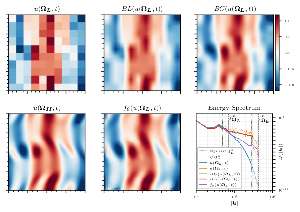
The energy spectrum is characteristic of the direct energy cascade observed in turbulent flows, a multi-scale phenomenon which sees energy content decaying with increasing wavenumber. In Figure 2, we observe that the energy content of the low-resolution field diverges from that of the high-resolution field; a consequence of spectral aliasing. Applying the de-aliasing rule to the Nyquist frequencies, we see that aliasing is introduced at for the low- and high-resolution fields respectively. This correlates with the divergence in energy content observed in the spectrum. We find that fields super-resolved by the network are capable of capturing finer scales of turbulence compared to low-resolution and interpolation approaches, prior to diverging at . This result is indicative of the impact of the residual-based loss, signifying the ability of the network to act beyond simple interpolation. The network is capable of de-aliasing, or inferring missing physics.
Despite the use of periodic padding in the convolutional layers, we observe artefacts on the boundaries of the predicted field. These artefacts are largely responsible for the divergence of the predicted energy spectrum from the true spectrum and provide a consideration for future work.
5 Conclusion
In this work, we have demonstrated the application of physics-informed CNNs for the super-resolution of the chaotic-turbulent Kolmogorov flow. Our results show improved performance when compared with standard interpolation methods. Evaluation of the turbulent energy spectrum highlights the ability of the network to resolve turbulent structures on a finer scale than available in the sparse observations. We note that this reconstruction of turbulence showcases the ability to resolve missing physics in the sparse observations, a consequence of embedding prior knowledge of the physics in the loss term. With a view on the spectral representation, we find that the network effectively mitigates the aliasing introduced by taking sparse observations. This work opens opportunities for the accurate reconstruction of dynamical systems from sparse observations, as is often the case in experimental settings for the physical sciences.
Acknowledgments and Disclosure of Funding
D. Kelshaw. and L. Magri. acknowledge support from the UK EPSRC. L. Magri gratefully acknowledges financial support from the ERC Starting Grant PhyCo 949388.
References
- Brunton et al. [2020] S. Brunton, B. Noack, and P. Koumoutsakos, “Machine learning for fluid mechanics,” Annual Review of Fluid Mechanics, vol. 52, pp. 477–508, 1 2020.
- Brunton et al. [2016] S. L. Brunton, J. L. Proctor, and J. N. Kutz, “Discovering governing equations from data by sparse identification of nonlinear dynamical systems,” Proceedings of the National Academy of Sciences, vol. 113, no. 15, pp. 3932–3937, 2016.
- Dong et al. [2014] C. Dong, C. C. Loy, K. He, and X. Tang, “Learning a deep convolutional network for image super-resolution,” in European Conference on Computer Vision, 2014, pp. 184–199.
- Shi et al. [2016] W. Shi, J. Caballero, F. Huszár, J. Totz, A. P. Aitken, R. Bishop, D. Rueckert, and Z. Wang, “Real-time single image and video super-resolution using an efficient sub-pixel convolutional neural network,” Proceedings of the IEEE Conference on Computer Vision and Pattern Recognition (CVPR), 9 2016.
- Yang et al. [2019] W. Yang, X. Zhang, Y. Tian, W. Wang, J.-H. Xue, and Q. Liao, “Deep learning for single image super-resolution: A brief review,” IEEE Transactions on Multimedia, vol. 21, pp. 3106–3121, 12 2019.
- Lagaris et al. [1998] I. E. Lagaris, A. Likas, and D. I. Fotiadis, “Artificial neural networks for solving ordinary and partial differential equations,” IEEE Transactions on Neural Networks, vol. 9, pp. 987–1000, 1998.
- Raissi et al. [2019] M. Raissi, P. Perdikaris, and G. E. Karniadakis, “Physics-informed neural networks: A deep learning framework for solving forward and inverse problems involving nonlinear partial differential equations,” Journal of Computational Physics, vol. 378, pp. 686–707, 2 2019.
- Cranmer et al. [2019] M. Cranmer, S. Greydanus, S. Hoyer, P. Battaglia, D. Spergel, and S. Ho, “Lagrangian neural networks,” in ICLR 2020 Workshop on Integration of Deep Neural Models and Differential Equations, 2019.
- Cai et al. [2021] S. Cai, Z. Mao, Z. Wang, M. Yin, and G. E. Karniadakis, “Physics-informed neural networks (pinns) for fluid mechanics: a review,” Acta Mechanica Sinica, vol. 37, pp. 1727–1738, 12 2021.
- Eivazi and Vinuesa [2022] H. Eivazi and R. Vinuesa, “Physics-informed deep-learning applications to experimental fluid mechanics,” 2022. [Online]. Available: https://arxiv.org/abs/2203.15402
- Liu et al. [2020] B. Liu, J. Tang, H. Huang, and X.-Y. Lu, “Deep learning methods for super-resolution reconstruction of turbulent flows,” Physics of Fluids, vol. 32, p. 25105, 2020.
- Gao et al. [2021] H. Gao, L. Sun, and J.-X. Wang, “Super-resolution and denoising of fluid flow using physics-informed convolutional neural networks without high-resolution labels,” Physics of Fluids, vol. 33, p. 073603, 7 2021.
- Fylladitakis [2018] E. D. Fylladitakis, “Kolmogorov flow: Seven decades of history,” Journal of Applied Mathematics and Physics, vol. 6, pp. 2227–2263, 2018.
- Canuto et al. [1988] C. Canuto, M. Y. Hussaini, A. Quarteroni, and T. A. Zang, Spectral Methods in Fluid Dynamics. Springer Berlin Heidelberg, 1988.
- Kim et al. [2016] J. Kim, J. K. Lee, and K. M. Lee, “Accurate image super-resolution using very deep convolutional networks,” in Proceedings of the IEEE Conference on Computer Vision and Pattern Recognition (CVPR), 2016.
- Simonyan and Zisserman [2015] K. Simonyan and A. Zisserman, “Very deep convolutional networks for large-scale image recognition,” in International Conference on Learning Representations, 2015.
- Li et al. [2018] H. Li, Z. Xu, G. Taylor, C. Studer, and T. Goldstein, “Visualizing the loss landscape of neural nets,” in Neural Information Processing Systems, 2018, pp. 6391–6401.