Validation of Stochastic Optimal Control Models for Goal-Directed Human Movements on the Example of
Human Driving Behavior

The human biomechanics and the system the human interacts with, e.g. a vehicle with steering wheel, is modeled via the linear time-discrete system dynamics

where $\bm{x}\in\mathbb{R}^{n}$ denotes the system state, $\bm{u}\in\mathbb{R}^{m}$ the control variable (typically neural activation of muscles), $\bm{y}\in\mathbb{R}^{r}$ the human observation and $\bm{A},\bm{B},\bm{H}$ matrices of appropriate dimension that may depend on time. When the additional time index $t$ is used, e.g. $\bm{x}_{t}$, the stochastic process of the corresponding variable is denoted. Furthermore, $\bm{\alpha}_{t}\in\mathbb{R}^{p}$ and $\bm{\varepsilon}_{t}=\left[\begin{matrix}\varepsilon_{t}^{(1)}&\dots&\varepsilon_{t}^{(c)}\end{matrix}\right]^{\top}$ are standard white Gaussian noise processes that constitute the additive and control-dependent noise process of state equation (1) with their scaling matrices $\bm{\Sigma}^{\bm{\xi}}$ and $\bm{C}_{i}=\sigma^{\bm{u}}_{i}\bm{B}\bm{F}_{i}$ of appropriate dimension. In (2), $\bm{\beta}_{t}\in\mathbb{R}^{q}$ and $\bm{\epsilon}_{t}=\left[\begin{matrix}\epsilon_{t}^{(1)}&\dots&\epsilon_{t}^{(d)}\end{matrix}\right]^{\top}$ are standard white Gaussian noise processes forming the additive and state-dependent noise process of the output equation with their corresponding scaling matrices $\bm{\Sigma}^{\bm{\omega}}$ and $\bm{D}_{i}=\sigma^{\bm{x}}_{i}\bm{H}\bm{G}_{i}$ of appropriate dimension. The stochastic processes $\bm{\alpha}_{t}$, $\bm{\varepsilon}_{t}$, $\bm{\beta}_{t}$ and $\bm{\epsilon}_{t}$ are independent to each other and to $\bm{x}_{t}$. The goal of the human, e.g. achievement of a desired steering angle under minimal effort, is modeled by the performance criterion

where $\bm{Q}_{N}$, $\bm{Q}$ and $\bm{R}$ are symmetric and of appropriate dimension. $\bm{Q}_{N}$, $\bm{Q}$ are positive semi-definite and $\bm{R}$ is positive definite. It is assumed that the human solves the LQS control problem consisting of the minimization of (3) with respect to (1) and (2) by an admissible control strategy. An approximate (suboptimal) solution to the LQS control problem is given by Todorov 2005 with $\bm{u}_{t}=-\bm{L}_{t}\hat{\bm{x}}_{t}$ and $\hat{\bm{x}}_{t+1}=\bm{A}\hat{\bm{x}}_{t}+\bm{B}\bm{u}_{t}+\bm{K}_{t}(\bm{y}_{t}-\bm{H}\hat{\bm{x}}_{t})+\bm{\eta}_{t}$, where $\bm{L}_{t}$ and $\bm{K}_{t}$ are computed by iterating between

and

In (4) and (5), $\bm{Z}_{t}^{\bm{e}}$, $\bm{Z}_{t}^{\bm{x}}$, $\bm{P}_{t}^{\bm{e}}$, $\bm{P}_{t}^{\hat{\bm{x}}}$, $\bm{P}_{t}^{\bm{e}\hat{\bm{x}}}$ and $\bm{P}_{t}^{\hat{\bm{x}}\bm{e}}$ follow from recursive equations (see Todorov 2005).

Suppose the cost function matrices $\bm{Q}_{N}$, $\bm{Q}$, $\bm{R}$ and the noise scaling parameters $\bm{\Sigma}^{\bm{\xi}}$, $\sigma_{i}^{\bm{u}}$, $\bm{\Sigma}^{\bm{\omega}}$, $\sigma_{i}^{\bm{x}}$ are known, the average human behavior (mean $\mathrm{E}\left\{\bm{x}_{t}\right\}$) and the human variability pattern (covariance $\bm{\Omega}_{t}^{\bm{x}}=\mathrm{cov}\left(\bm{x}_{t},\bm{x}_{t}\right)=\mathrm{cov}\left(\bm{x}_{t}\right)$) predicted by the LQS model are given by Lemma 1.

See (Karg et al. 2022, Lemma 2).

From (6) and (8) the dependency of $\mathrm{E}\left\{\bm{x}_{t}\right\}$ on $\bm{L}_{t}$ (4) follows. In the fully observable case, $\bm{Z}_{t}^{\bm{e}}$ drops out in (4) (see Todorov 2005) but $\bm{L}_{t}$ still depends on $\bm{C}_{i}$ and thus $\sigma_{i}^{\bm{u}}$. In the partially observable case, the additional dependencies follow from the dependency of $\bm{L}_{t}$ on $\bm{Z}_{t}^{\bm{e}}$ which in turn depends on $\bm{K}_{t}$ (see Todorov 2005).

Corollary 1 shows that the human average behavior $\mathrm{E}\left\{\bm{x}_{t}\right\}$ predicted by the LQS model depends not only on the cost function matrices but also on the scaling parameters of the noise processes. Hence, they could act as a crucial part of the LQS model improving the performance in describing human average behavior.

Regarding the LQS model introduced in the previous section, the cost function matrices $\bm{Q}_{N}$, $\bm{Q}$, $\bm{R}$ and the noise (scaling) parameters $\bm{\Sigma}^{\bm{\xi}}$, $\sigma_{i}^{\bm{u}}$, $\bm{\Sigma}^{\bm{\omega}}$, $\sigma_{i}^{\bm{x}}$ are unknown and need to be identified when looking at human movements in practice. To simplify notation, we combine the cost function parameters in a vector $\bm{s}\in\mathbb{R}^{S}$ and the noise parameters in a vector $\bm{\sigma}\in\mathbb{R}^{\Sigma}$ (see Karg et al. 2022). Now, we assume that our measurement data consists of a set $\{\bm{M}\bm{x}^{\ast,(k)}_{t}\}$ ($k\in\{1,\dots,K\}$) of time-discrete trajectories $\bm{M}\bm{x}^{\ast,(k)}_{t}$ where $\bm{x}^{\ast,(k)}_{t}$ is a realization of the stochastic process $\bm{x}_{t}^{\ast}$. It results in the closed-loop LQS system with the unknown cost function $\bm{s}^{\ast}$ and noise parameters $\bm{\sigma}^{\ast}$ of the human. With $\bm{M}\in\mathbb{R}^{\bar{n}\times n}$, we consider that not all system states are measured, i.e. $\bm{M}$ follows from the identity matrix by deleting rows corresponding to not measured states. The identification problem is finally formalized in Problem 1¹¹ 1 The problem extends typical Inverse Optimal Control or Inverse Reinforcement Learning problems by additionally searching for scaling parameters of noise processes..

In order to solve Problem 1, we have introduced an ISOC algorithm based on two bi-level optimizations in our previous work (Karg et al. 2022). We formulate a direct optimization problem by defining a performance criterion $J_{\ISOC}$ describing how well the mean $\mathrm{E}\left\{\bm{x}_{t}\right\}$ and covariance $\bm{\Omega}_{t}^{\bm{x}}$ predicted by the LQS model with parameters $\bm{s}$ and $\bm{\sigma}$ match the measurement data $\hat{\bm{m}}_{t}$ and $\hat{\bm{\Omega}}_{t}^{\bm{x}^{\ast}}$. The objective function $J_{\ISOC}$ is chosen based on the Variance Accounted For (VAF) metric:

where for the elements $m^{\text{VAF}}_{i}$ and $\Omega^{\text{VAF}}_{ij}$

holds. In (10), $\bm{w}_{\text{m}}\in\mathbb{R}^{\bar{n}}$ and $\bm{w}_{\text{v}}\in\mathbb{R}^{\bar{n}\bar{n}}$ denote weighting vectors. Due to the VAF metric $J_{\ISOC}\in(-\infty,1]$ holds with $1$ corresponding to a perfect fit between predicted and measured data. Therefore, the direct ISOC optimization problem consists of maximizing $J_{\ISOC}$: $\max\limits_{\bm{s},\bm{\sigma}}\left(J_{\ISOC}\left(\hat{\bm{m}}_{t},\hat{\bm{\Omega}}^{\bm{x}^{\ast}}_{t},\mathrm{E}\left\{\bm{x}_{t}\right\},\bm{\Omega}^{\bm{x}}_{t}\right)\right)$. The evaluation of $J_{\ISOC}$ with specific values for $\bm{s}$ and $\bm{\sigma}$ depends on calculating the model predictions $\mathrm{E}\left\{\bm{x}_{t}\right\}$ and $\bm{\Omega}_{t}^{\bm{x}}$ which in turn depends on solving the forward optimal control problem, i.e. computing $\bm{K}_{t}$ and $\bm{L}_{t}$. Hence, maximizing $J_{\ISOC}$ leads to a bi-level optimization problem where the upper level optimization consists of maximizing $J_{\ISOC}$ and the lower level of calculating $\bm{K}_{t}$, $\bm{L}_{t}$, $\mathrm{E}\left\{\bm{x}_{t}\right\}$ and $\bm{\Omega}_{t}^{\bm{x}}$. In order to keep this optimization computationally tractable, we apply an alternating optimization approach by computing the best estimate $\tilde{\bm{s}}^{(l)}$ for a given estimate $\tilde{\bm{\sigma}}^{(l-1)}$ in the first step of one iteration $l$ and in the second vice versa. This leads to the iteration between two bi-level optimizations shown in Fig. 1. Furthermore, in the lower levels of both bi-level optimizations our newly introduced Lemma 1 is utilized to simplify the computation of $\mathrm{E}\left\{\bm{x}_{t}\right\}$ and $\bm{\Omega}_{t}^{\bm{x}}$ by applying recursive calculations only. Finally, for solving the upper level optimizations the parameters $\bm{s}$ and $\bm{\sigma}$ are divided into parameter sets where each parameter is supposed to be in at least one set and where the parameters in one set are assumed to have a mutually correlated influence on $J_{\ISOC}$. Then, grid searches with fixed grid size are performed on these parameter sets iteratively until no further improvement with the current grid size is achieved. Then, the grid size is shrinked. Further details regarding the ISOC algorithm can be found in (Karg et al. 2022).

The human measurement data was gathered by a study where 14 participants (12 male and 2 female subjects) aged between 19 and 29 (24.9 in average) performed a simplified steering task. The participants interacted with an active steering wheel which was equipped with an incremental encoder (40000 steps per full rotation) to measure the steering angle $\varphi$ with a sampling frequency of $100\text{\,}\mathrm{H}\mathrm{z}$. Based on the steering angle measurements torque was applied by the steering wheel such that it mimicked the dynamics of a spring-damper system. With the steering wheel the participants were able to move a marker (square) on a screen on a horizontal line with fixed vertical position (cf. Figure 2). The horizontal position of the marker was a linear mapping of the steering angle.

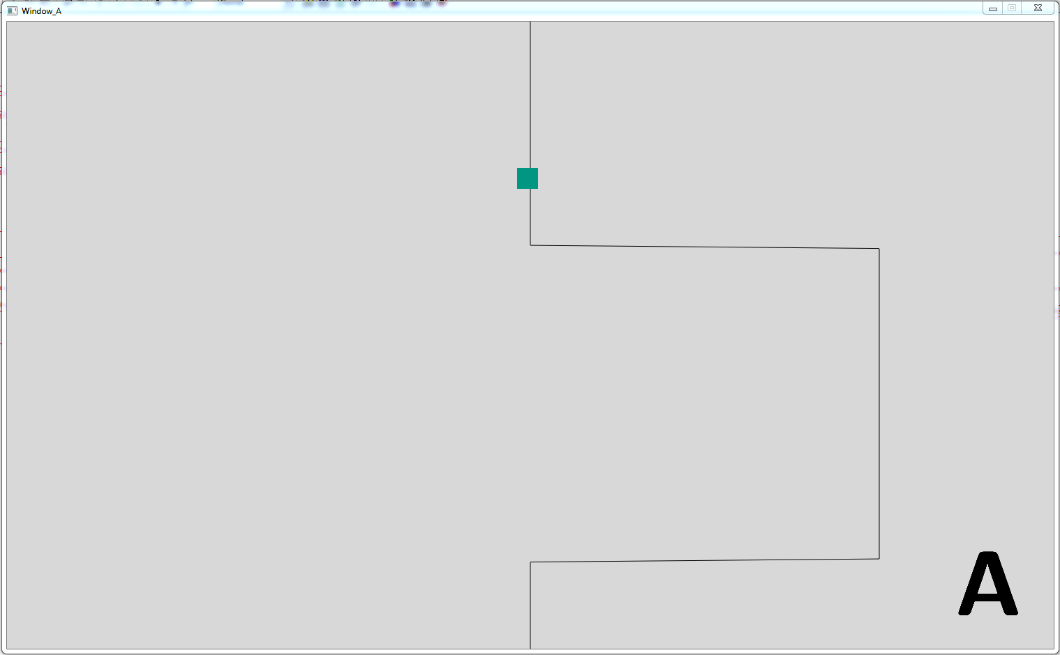
On the display, a reference trajectory for the marker (cf. Figure 2) was shown and the participants were asked to follow it as best as possible. The reference trajectory moved downwards with constant velocity. The reference trajectory shown for the marker is directly connected to a reference trajectory $\varphi_{\text{r},t}$ for the steering angle. The trial of one participant started with a familiarization phase of $210\text{\,}\mathrm{s}$ consisting of different segments with a steering angle reference with constant curvature where the curvature varied between those segments. Afterwards, the reference consisted of 14 repetitions of the same piecewise constant pattern: $\varphi_{\text{r}}=0$, $\varphi_{\text{r}}=+\frac{2}{3}\pi$, $\varphi_{\text{r}}=0$ and $\varphi_{\text{r}}=-\frac{2}{3}\pi$, each for a duration of $100$ time steps.

Regarding the data preparation, we first applied a cubic spline smoothing on the measured steering angle to reduce measurement noise. Afterwards, we calculate the steering angle velocity $\dot{\varphi}_{t}$ via numerical differentiation. Since the measured data consists of 14 repetitions of the $+\frac{2}{3}\pi$-step as well as 14 repetitions of the $-\frac{2}{3}\pi$-step, we calculate estimates of human average behavior ($\hat{\bm{m}}_{t}$) and human variability pattern ($\hat{\bm{\Omega}}_{t}^{\bm{x}^{\ast}}$) for each of these movements from the corresponding 14 repetitions. Hereto, we determine the starting time for each single movement repetition as the last point in time where $\varphi\approx 0$ and $\dot{\varphi}<$0.1\text{\,}\mathrm{s}^{-1}$$ holds. In some segments with $\varphi_{\text{r}}=0$ the steering angle velocity is always above this threshold. Then, we increase the threshold in $0.01\text{\,}\mathrm{s}^{-1}$-steps until a maximum value of $0.4\text{\,}\mathrm{s}^{-1}$. If even this maximally relaxed condition is not fulfilled, we remove this single movement repetition from the further analysis since the human clearly starts not from an equilibrium condition in this case. Finally, the remaining repetitions are used to calculate the mean ($\hat{\bm{m}}_{t}$) and covariance estimate ($\hat{\bm{\Omega}}_{t}^{\bm{x}^{\ast}}$) of $\varphi_{t}$ and $\dot{\varphi}_{t}$. The movement duration is defined as the averaged movement duration of those repetitions which fulfill the condition for a movement ending ($\varphi\approx\pm\frac{2}{3}\pi$ and $\dot{\varphi}<$0.1\text{\,}\mathrm{s}^{-1}$$). This data preparation is done for every subject.

Fig. 3 shows the steering angle velocity profiles for the $+\frac{2}{3}\pi$-step achieved by the averaging procedure described before. Remarkably, the profiles possess very similar kinematic features as point-to-point reaching movements: they are all single-peaked and predominantly bell-shaped and nearly symmetric. The majority of the profiles is furthermore slightly left-skewed which indicates that the subjects tend to perform fast movements (Engelbrecht 2001). Moreover, the maximum to mean ratios of $\mathrm{E}\left\{\dot{\varphi}\right\}$ range from $1.78$ to $2.26$ (when S10 is not considered due to its outlier behavior). All these features were also observed for point-to-point human hand movements (Engelbrecht 2001). This conclusion shows on one side the validity of our measured data and on the other that we can make a first step towards a data-driven validation of SOC models for general goal-directed human movements by applying our ISOC algorithm.

Before results of this application are presented in the next section, the system equations (1) and (2) need to be set up for the driving experiment. The active steering wheel is modeled by the spring-damper dynamics

where $M_{\text{h}}$ is the steering torque applied by the human. It results from a second-order linear filter with time constants $\tau_{1}$ and $\tau_{2}$ describing the low-pass characteristics of the muscle dynamics (Winter 1990):

where $u$ is the neural activation and $g$ the muscle excitation. We define the system state as $\bm{x}=\left[\begin{matrix}\varphi&\dot{\varphi}&M_{\text{h}}&g&\varphi_{\text{r}}\end{matrix}\right]^{\top}$. The augmentation of it with the target steering angle $\varphi_{\text{r}}$ (constant dynamics) is a mathematical reformulation to consider target steering angles $\varphi_{\text{r}}\neq 0$ but still constitute the cost function in the form of (3):

from which the definition of the cost function vector $\bm{s}$ follows. Discretizing (13) and (14) and choosing the numerical values as $\Theta=$0.056\text{\,}\mathrm{k}\mathrm{g}\mathrm{m}^{2}$$, $c=$1.146\text{\,}\mathrm{N}\mathrm{m}$$, $d=$0.859\text{\,}\mathrm{N}\mathrm{m}\mathrm{s}$$ and $\tau_{1}=\tau_{2}=$0.04\text{\,}\mathrm{s}$$ yields $\bm{A}$ and $\bm{B}$. Furthermore, $\bm{H}=\left[\begin{matrix}\bm{I}_{3\times 3}&\bm{0}_{3\times 2}\end{matrix}\right]$ is assumed for the human perception since $\varphi_{\text{r}}$ only results from the above mentioned mathematical reformulation and $g$ cannot be clearly associated with the human sensory apparatus. Due to lack of further knowledge about the additive noise processes and to keep the number of noise parameters tractable, independent stochastic processes $\alpha_{i,t}$ and $\beta_{i,t}$ are modeled for every state and output: $\bm{\Sigma}^{\bm{\xi}}=\diag(\left[\begin{matrix}\sigma_{1}&\sigma_{2}&\sigma_{3}&\sigma_{4}&0\end{matrix}\right])$ and $\bm{\Sigma}^{\bm{\omega}}=\diag(\left[\begin{matrix}\sigma_{5}&\sigma_{6}&\sigma_{7}\end{matrix}\right])$. Finally, the signal-dependent noise processes are modeled by $\bm{C}=\sigma_{8}\bm{B}$ (single-input system), $\bm{D}_{1}=\sigma_{9}\bm{H}\diag(\left[\begin{matrix}1&0&0&0&0\end{matrix}\right])$, $\bm{D}_{2}=\sigma_{10}\bm{H}\diag(\left[\begin{matrix}0&1&0&0&0\end{matrix}\right])$ and $\bm{D}_{3}=\sigma_{11}\bm{H}\diag(\left[\begin{matrix}0&0&1&0&0\end{matrix}\right])$ which completes the definition of the noise parameter vector $\bm{\sigma}$. Again, due to lack of further knowledge about the state-dependent noise processes, the $\bm{G}_{i}$ are chosen such that every perceived state is influenced by an independent noise process scaled by the corresponding state. In case of the LQG and LQ model, the signal-dependent and all noise parameters drop out, respectively.

For applying our ISOC algorithm, we first divide the measurement data into training and validation data. The parameters $\bm{s}$ and $\bm{\sigma}$ of the LQS, LQG and LQ model are identified for each subject individually with $\hat{\bm{m}}_{t}$ and $\hat{\bm{\Omega}}_{t}^{\bm{x}^{\ast}}$ calculated from the repetitions of the $+\frac{2}{3}\pi$-step. Here, we set $\bm{M}=\left[\begin{matrix}\bm{I}_{2\times 2}&\bm{0}_{2\times 3}\end{matrix}\right]$ since $\varphi$ and $\dot{\varphi}$ are measured. The repetitions of the $-\frac{2}{3}\pi$-step serve as validation data, i.e. the corresponding values for $\hat{\bm{m}}_{t}$ and $\hat{\bm{\Omega}}_{t}^{\bm{x}^{\ast}}$ are the ground truth data for the LQS, LQG and LQ model predictions computed with $\tilde{\bm{s}}$ and $\tilde{\bm{\sigma}}$. The weighting vectors for the cost function bi-level optimization are chosen as $\bm{w}_{\text{m}}=\left[\begin{matrix}0.9&0.9\end{matrix}\right]^{\top}$ and $\bm{w}_{\text{v}}=\left[\begin{matrix}0.1&0\end{matrix}\right]^{\top}$ in case of the LQS and LQG model and as $\bm{w}_{\text{m}}=\left[\begin{matrix}1&1\end{matrix}\right]^{\top}$ and $\bm{w}_{\text{v}}=\left[\begin{matrix}0&0\end{matrix}\right]^{\top}$ for the LQ model. For the noise parameter bi-level optimization in case of the LQS and LQG model, $\bm{w}_{\text{m}}=\left[\begin{matrix}0.1&0.1\end{matrix}\right]^{\top}$ and $\bm{w}_{\text{v}}=\left[\begin{matrix}0.9&0\end{matrix}\right]^{\top}$ holds.

References

- Engelbrecht (2001) Engelbrecht, S. (2001). Minimum principles in motor control. Journal of Mathematical Psychology, 45, 497–542.
- Flash and Hogan (1985) Flash, T. and Hogan, N. (1985). The coordination of arm movements: An experimentally confirmed mathematical model. The Journal of Neuroscience, 5(7), 1688–1703.
- Franklin and Wolpert (2011) Franklin, D.W. and Wolpert, D.M. (2011). Computational mechanisms of sensorimotor control. Neuron, 72(3), 425–442.
- Gallivan et al. (2018) Gallivan, J.P., Chapman, C.S., Wolpert, D.M., and Flanagan, J.R. (2018). Decision-making in sensorimotor control. Nature Reviews. Neuroscience, 19(9), 519–534.
- Harris and Wolpert (1998) Harris, C.M. and Wolpert, D.M. (1998). Signal-dependent noise determines motor planning. Nature, 394, 780–784.
- Karg et al. (2021) Karg, P., Kalb, L., Bengler, K., and Hohmann, S. (2021). Passing the baton between autopilot and driver. ATZ Worldwide, 123, 68–72.
- Karg et al. (2022) Karg, P., Stoll, S., Rothfuß, S., and Hohmann, S. (2022). Inverse stochastic optimal control for linear-quadratic gaussian and linear-quadratic sensorimotor control models. IEEE Conference on Decision and Control, 2801–2808.
- Kolekar et al. (2018) Kolekar, S., Mugge, W., and Abbink, D. (2018). Modeling intradriver steering variability based on sensorimotor control theories. IEEE Transactions on Human-Machine Systems, 48(3), 291–303.
- MacAdam (1981) MacAdam, C.C. (1981). Application of an optimal preview control for simulation of closed-loop automobile driving. IEEE Transactions on Systems, Man, and Cybernetics, 11(6), 393–399.
- Markkula (2014) Markkula, G. (2014). Modeling driver control behavior in both routine and near-accident driving. Human Factors and Ergonomics Society Annual Meeting, 58(1), 879–883.
- Nash and Cole (2015) Nash, C.J. and Cole, D.J. (2015). Development of a novel model of driver-vehicle steering control incorporating sensory dynamics. Dynamics of Vehicles on Roads and Tracks, 72–81.
- Ross and Bagnell (2010) Ross, S. and Bagnell, J.A. (2010). Efficient reductions for imitation learning. International Conference on Artificial Intelligence and Statistics, 661–668.
- Sentouh et al. (2009) Sentouh, C., Chevrel, P., Mars, F., and Claveau, F. (2009). A sensorimotor driver model for steering control. IEEE International Conference on Systems, Man, and Cybernetics, 2462–2467.
- Todorov (2004) Todorov, E. (2004). Optimality principles in sensorimotor control. Nature Neuroscience, 7(9), 907–915.
- Todorov (2005) Todorov, E. (2005). Stochastic optimal control and estimation methods adapted to the noise characteristics of the sensorimotor system. Neural Computation, 17, 1084–1108.
- Todorov and Jordan (2002) Todorov, E. and Jordan, M.I. (2002). Optimal feedback control as a theory of motor coordination. Nature Neuroscience, 5(11), 1226–1235.
- Uno et al. (1989) Uno, Y., Kawato, M., and Suzuki, R. (1989). Formation and control of optimal trajectory in human multijoint arm movement. Biological Cybernetics, 61, 89–101.
- Winter (1990) Winter, D.A. (1990). Biomechanics and Motor Control of Human Movement. Wiley, 2nd edition.