The miniJPAS survey: stellar atmospheric parameters from 56 optical filters2022The miniJPAS survey: stellar atmospheric parameters from 56 optical filters–References
Abstract
With a unique set of 54 overlapping narrow-band and two broader filters covering the entire optical range, the incoming Javalambre-Physics of the Accelerating Universe Astrophysical Survey (J-PAS) will provide a great opportunity for stellar physics and near-field cosmology. In this work, we use the miniJPAS data in 56 J-PAS filters and 4 complementary SDSS-like filters to explore and prove the potential of the J-PAS filter system in characterizing stars and deriving their atmospheric parameters. We obtain estimates for the effective temperature with a good precision (150 K) from spectral energy distribution fitting. We have constructed the metallicity-dependent stellar loci in 59 colours for the miniJPAS FGK dwarf stars, after correcting certain systematic errors in flat-fielding. The very blue colours, including , , , , show the strongest metallicity dependence, around 0.25 mag/dex. The sensitivities decrease to about 0.1 mag/dex for the , , and colours. The locus fitting residuals show peaks at the , and filters, suggesting that individual elemental abundances such as [Ca/Fe], [C/Fe], and [Mg/Fe] can also be determined from the J-PAS photometry. Via stellar loci, we have achieved a typical metallicity precision of 0.1 dex. The miniJPAS filters also demonstrate strong potential in discriminating dwarfs and giants, particularly the and filters. Our results demonstrate the power of the J-PAS filter system in stellar parameter determinations and the huge potential of the coming J-PAS survey in stellar and Galactic studies.
Keywords:
stars:fundamental parameters – stars:abundances – techniques:photometric – methods:statistical1 Introduction
The Javalambre-Physics of the Accelerating Universe Astrophysical Survey (Benitez et al. 2014, J-PAS;) aims to image 8500 square degrees of the northern sky with a unique set of 54 overlapping narrow-band filters and 2 broad-band filters, with a dedicated 2.5-m telescope, JST/T250, at the Observatorio Astrofísico de Javalambre (Cenarro et al. 2014, OAJ;). The narrow-band filters have a tpyical FWHM of 145 Å, covering the entire optical range from 3785 to 9100 Å. Driven by accurate redshift estimates of galaxies over a wide range of epochs, the J-PAS survey will effectively deliver a low-resolution spectra for every single pixel of the 8500 deg2 sky area observed, providing valuable datasets for not only cosmology and galaxy evolution, but also stellar physics and near-field cosmology.
As a pathfinder for J-PAS, the miniJPAS survey (Bonoli et al. 2021) has imaged the famous Extended Groth Strip (EGS) field of about 1 deg2, with the JPAS-Pathfinder (JPF) camera. In addition to test the performance of the telescope, the miniJPAS data offers a great opportunity to prove the potential of the J-PAS filter system. In this work, we explore the power of these filters in characterizing stars and deriving their fundamental parameters via different techniques.
Metallicity-dependent stellar locus (Yuan et al. 2015a) provides a simple yet non-trivial tool to investigate the dependencies of colours on metallicity and to determine the metallicity for millions of stars from multi-band photometry. Yuan et al. 2015b applied this technique to the re-calibrated Sloan Digital Sky Survey (York et al. 2000, SDSS;) SDSS/Stripe 82 (Yuan et al. 2015c) and obtained metallicities for half a million FGK dwarf stars, with a typical error of [Fe/H] 0.1-0.2 dex. Using the same data, Zhang et al. 2021 obtained metallicity-dependent stellar loci for red-giant stars and used them to derive metallicities of giants to a precision of [Fe/H] 0.20-0.25 dex, and to discriminate metal-poor red giants from main-sequence stars based on SDSS photometry. With the recalibrated SkyMapper Southern Survey (SMSS) DR2 (Huang et al. 2021), Huang et al. 2022 determined metallicities for over 24 million stars with a similar technique, achieving a precision comparable to or slightly better than that derived from spectroscopy for stars with metallicities as low as [Fe/H] . Based on corrected broad-band Gaia Early Data Release 3 (Gaia Collaboration et al. 2016; Gaia Collaboration et al. 2021, Gaia EDR3;) colours alone by Niu et al. 2021b and Yang et al. 2021, and a careful reddening correction, Xu et al. 2022 determined reliable metallicity estimates for a magnitude-limited sample of about 27 million stars down to [Fe/H] = .
In this work, we first determine effective temperatures via spectral energy distribution (SED) fitting, based on miniJPAS photometry. We then investigate the dependencies of miniJPAS colours on the metallicity and perform [Fe/H] estimates for FGK dwarf stars via the metallicity-dependent stellar loci. At last, we explore giant/dwarf classifications using a machine learning technique to identify the most sensitive colours. Note that measurements of surface gravity are not discussed in this work.
This paper is organized as follows: Section 2 describes the miniJPAS data used in this work. Section 3 presents the stellar characterization using the available photometric data. The metallicity-dependent stellar loci are determined and discussed in Section 4. Metallicity estimates are described and compared in Section 5 and Section 6 discusses giant/dwarf classifications. Finally, we summarize our work in Section 7.
2 MiniJPAS Data
The miniJPAS was carried out at OAJ with the JPF camera mounted on the JST/T250 telescope. JPF was the first scientific instrument of the JST/T250, before the arrival of the Javalambre Panoramic Camera (Taylor et al. 2014; Marín-Franch et al. 2017, JPCam;). The JPF has a single 92009200 CCD, located at the center of the JST250 field of view (FoV), with a pixel scale of 0.23 arcsec pixel-1, providing an effective FoV of 0.27 deg2.
In addition to the 54 narrow-band filters, ranging from 3785 to 9100 Å, two broader filters, (also known as , that covers the ultraviolet edge) and (that covers the red wings), and four SDSS-like broad-band filters (, , , and ) are also used. The J-PAS filters have been optimized to deliver a low-resolution () photo-spectrum of each imaged pixel/target, therefore probing a large number of key stellar absorption features. The technical description and characterization of the J-PAS filters can be found in Marín-Franch et al. 2012. Detailed information of the filters as well as their transmission curves are available at the Spanish Virtual Observatory Filter Profile Service11 1 http://svo2.cab.inta-csic.es/theory/fps/index.php?mode=browse&gname=OAJ&gname2=JPAS.
The miniJPAS covers the Extended Groth Strip area at (, ) = (215, 53) deg with four tiles, with a total area of about 1 deg2 (see Bonoli et al. 2021, for further details). All data collected are processed and calibrated by the Data Processing and Archiving Unit group at CEFCA22 2 Centro de Estudios de Física del Cosmos de Aragón (Spain).. The image depths achieved – 5 in a 3 arcsec circular aperture -- are deeper than 22 mag for filters bluewards of 7500Å and about 22 mag for longer wavelengths. The images and catalogues are publicly available on the J-PAS website33 3 http://www.j-pas.org/datareleases/minijpas_public_data_release_pdr201912. The 6 arcsec-aperture magnitudes in the “dual mode” catalogues are used in this work, along with aperture corrections. In the “dual mode”, the -band images were used to detect targets with SExtractor (Bertin & Arnouts 1996), and the apertures defined then were also used in other filters.
We select stars from the miniJPAS database that fulfill the following criteria: 22 mag and CLASS_STAR44 4 Morphological classification parameter provided by SExtractor 0.6. A number of 2895 stars are selected, including 1566 and 749 stars brighter than 20 and 18 magnitude in the band, respectively. The selected stars are cross-matched with the LAMOST DR7 (Luo et al. 2015) with a match radius of 1 arcsec, 161 common stars are found, including 10 giant stars. The selected stars are also cross-matched with the SDSS/SEGUE catalog (Rockosi et al. 2022), with only 31 stars found. We also cross-match the selected stars with the J-PLUS DR1 stellar parameters catalogue from Yang et al. 2022, 682 stars of are found. Given the small number of common stars between the miniJPAS catalogue with LAMOST or SDSS spectroscopic catalogues, we have adopted different approaches to characterize the stellar miniJPAS sample, which will be described in the following sections.
3 Stellar effective temperature from SEDs
3.1 SED fitting with VOSA


We used the Virtual Observatory Sed Analyzer55 5 http://svo2.cab.inta-csic.es/theory/vosa/ (Bayo et al. 2008, VOSA;) and the SEDs constructed from the miniJPAS photometry data, to obtain the stellar effective temperatures () of the objects in the miniJPAS survey via atmospheric model fitting. We used the BT-Settl spectra models by Allard et al. 2011, computed with a cloud model, for all available temperatures – from 400 K to 70 000 K, with a pace of 100 K till the 7 000 K, then a pace of 200 K till the 12 000 K, increasing the pace to 500 K till the 12 000,̨ and with a final pace of 1000 K for temperatures larger than 20 000 K – with log varying from 2.0 to 6.0 dex and the metallicity ([M/H]) from 4.0 to 0.5, both with a pace of 0.5. VOSA also allows to work with a range of extinctions. We set this range from =0 to 0.1, the maximum Milky Way extinction in the region of the sky covered by the miniJPAS (Bonoli et al. 2021). VOSA unreddens the miniJPAS SEDs using 20 values of within this range in steps of 0.005 mag, and selected the value which unreddened SED best fit the model. It is worth mentioning that fit parameter uncertainties are estimated in VOSA by performing a Monte Carlo simulation with a 100 iterations. Taking the observed SED as the starting point, VOSA generates 100 virtual SEDs introducing a Gaussian random noise for each point proportional to the observational error. VOSA obtains the best fit for the 100 virtual SEDs with noise and makes the statistics for the distribution of the obtained values for each parameter. The standard deviation for this distribution will be reported as the uncertainty for the parameter if its value is larger that half the grid step for this parameter.
The complete miniJPAS stellar sample contains 2 895 objects. We constructed the SEDs only with good photometric data (individual filter photometry flag4). This translated in 2 871 miniJPAS SEDs constructed using between 1 and 60 photometry bands (including the four SDSS-like filters). However, considering the variables on the fitting procedure, a minimum of 6 photometric points are needed to perform the fit, which reduced the sample to 2 858 SEDs, most of them (>94%) with at least 50 photometric points.
From the 2 858 analysed SEDs, we found a good-fit solution – defined by a modified reduced value (66 6 Vgfb: Modified reduced , calculated by forcing to be larger than , where is the error in the observed flux (). This can be useful if the photometric errors of any of the catalogues used to build the SED are underestimated. Vgfb smaller than 10–15 is often perceived as a good fit. http://svo2.cab.inta-csic.es/theory/vosa/help/star/fit/.) of less than 3 – for 2 732 of them, representing 95% of the miniJPAS analysed sample. To illustrate, Figure 1 shows two examples of obtained SED fittings, the one with the lowest , and a rejected solution, close to the cutoff limit of =3.
The temperatures obtained range from 2 700 to 19 000 K. Figure 2 shows the distribution obtained from VOSA for the sample with best SED fitting results – 2 732 objects with . The distribution is consistent with what is expected from a field stellar sample, in which dwarfs and giants are present (Van der Swaelmen et al. 2022).
3.2 The LAMOST control sample
In order to evaluate both the accuracy of the fitting method and the reliability of the derived effective temperature, we compare the VOSA results with the effective temperature derived from spectroscopy. We cross-matched the miniJPAS stellar sample with the LAMOST DR7 catalogue (Luo et al. 2015), finding 151 LAMOST objects for which we obtained a good fit with VOSA.
Figure 3 (top panel) shows the comparison between the obtained by miniJPAS SED fitting with VOSA, and those obtained from spectroscopy by LAMOST. We found a good agreement, within uncertainties, with the SED fitting temperatures slightly cooler than the spectroscopic ones.


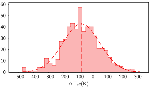
Figure 3 (bottom panel) shows the distribution of the difference in between the values obtained from the miniJPAS SED fitting with VOSA and those from LAMOST spectroscopy, after removing the 3- clipped outliers. We fitted the distribution to a Gaussian curve, resulting in a mean value of 60 K and a standard deviation of 103 K, approximately. From this, and considering that the LAMOST uncertainties have a median value of 60 K, we can conservatively estimate a typical uncertainty lower than 150 K in the VOSA miniJPAS SED fitting, in the range of temperatures in common. This result validates the miniJPAS data set and the SED fitting methodology with VOSA as a reliable way to obtain stellar effective temperatures for thousands of sources, without the need of more resource demanding spectroscopic observations.
From the analysed LAMOST sample, we reached the conclusion that even with the amazing collection of 56 narrow-band filters, there is not enough resolution in the SED to derive surface gravities and metallicities with good precision. This result was expected as SEDs have much lower sensitivity to changes in logg and metallicity. Therefore, other approaches are presented below.
3.3 J-PLUS stellar sample


Given the small numbers of stars in common between the miniJPAS catalogue and the LAMOST/SDSS spectroscopic catalogues, we further used the J-PLUS stellar parameters from Yang et al. 2022 to compare with our miniJPAS SED fitting results. The J-PLUS DR1 catalogue was re-calibrated with the stellar colour regression method (Yuan et al. 2015c; Huang et al. 2021; Niu et al. 2021a; Niu et al. 2021b; Huang & Yuan 2022; Xiao & Yuan 2022), achieving a calibration precision of 2-5 mmag in all 12 J-PLUS filters. Based on the re-calibrated JPLUS DR1 and Gaia DR2 (Gaia Collaboration et al. 2018), Yang et al. 2022 trained 8 cost-sensitive neural networks, the CSNet, to learn the non-linear mapping from stellar colours to their labels independently. The stellar parameter achieved internal precisions were of 55 K for , about 0.15 dex for log , and 0.07 dex for [Fe/H], respectively. Abundance for [/Fe] and 4 individual elements ([C/Fe], [N/Fe], [Mg/Fe], and [Ca/Fe]) were also estimated, with a precision of 0.04-0.08 dex. The catalogue containing about 2 million stars is publicly available77 7 http://www.j-plus.es/ancillarydata/index.
We cross-matched J-PLUS DR1 stellar parameters catalogue from Yang et al. 2022 with the miniJPAS sample with good-fitting result from VOSA (2 732 objetcs). A total of 542 stars were found in common. The obtained VOSA temperatures (this work) are in a very good agreement with the previous results by Yang et al. 2022, as illustrated in Figure 4, where both results are compared. The obtained from the miniJPAS SED fitting with VOSA are presented in the abscissa axis. The temperatures by Yang et al. 2022 are presented in the ordinate axis (top panel), showing the accordance in respect to the identity function (black line). The difference between both results, this work and the results by Yang et al. 2022, are also shown (bottom panel). After applying a 3- clipping, we found a mean difference of 81 K, with a standard deviation () of 124 K, approximately. These results are in complete agreement, within the estimated errors, to those obtained in the comparison to LAMOST data, being VOSA slightly cooler in the 48005800 K range. Probably, this trend is due to different systematics between the VOSA and J-PLUS/LAMOST results, since Yang et al. 2022 used LAMOST data for training the artificial neural networks and the same behavior is seen when comparing the SED obtained from VOSA to those from LAMOST spectra (see fig. 3, top panel).
The versus (gi)0 diagram is presented in Figure 5, where black diamonds show the temperatures obtained from VOSA analysis for the miniJPAS SEDs. Note that only those stars with 10 000 K are presented. For comparison, the temperatures obtained by Yang et al. 2022 are also shown, represented by red filled circles. This figure shows that VOSA follows a similar trend with the (gi)0 colour to the one found by Yang et al. 2022, but extending to a wider range of temperatures. This, again, validate our methodology to derive effective temperatures for thousands of sources from miniJPAS SEDs with VOSA.
4 Metallicity-dependent stellar loci of FGK dwarf stars
We also used the Yang et al. 2022 J-PLUS DR1 stellar parameter estimations to determine the metallicity-dependent stellar loci of the miniJPAS colours for FGK dwarf stars. After requiring < 1.6, 4000 < < 7000 K, > 4.0, and flag = 0 in all the miniJPAS filters, 310 FGK dwarf stars of high-quality photometry and stellar parameters are selected. These stars, including 10 with [Fe/H] , are used to determine the metallicity-dependent stellar loci of the miniJPAS colours.
| Filter | ||||||
|---|---|---|---|---|---|---|
| uJAVA | 0.0372 | 1.65e-06 | 4.47e-10 | 1.20e-05 | 1.29e-10 | 6.57e-10 |
| J0378 | 0.0778 | 8.89e-06 | 4.46e-10 | 1.95e-05 | 4.22e-10 | 1.22e-09 |
| J0390 | 0.0770 | 1.77e-06 | 2.38e-10 | 2.01e-05 | 1.05e-10 | 9.81e-10 |
| J0400 | 0.0391 | 2.75e-06 | 2.59e-10 | 9.07e-06 | 2.19e-10 | 4.74e-10 |
| J0410 | 0.0256 | 1.84e-06 | 2.72e-10 | 5.84e-06 | 4.05e-10 | 2.76e-10 |
| J0420 | 0.0286 | 4.19e-07 | 4.51e-11 | 7.84e-06 | 2.53e-10 | 5.75e-10 |
| J0430 | 0.0313 | 4.15e-06 | 2.85e-10 | 4.71e-06 | 1.04e-10 | 1.16e-10 |
| J0440 | 0.0291 | 2.92e-06 | 1.16e-10 | 5.79e-06 | 5.99e-11 | 2.30e-10 |
| J0450 | 0.0093 | 2.30e-06 | 2.15e-10 | 2.19e-06 | 2.81e-10 | 3.94e-11 |
| J0460 | 0.0137 | 7.36e-07 | 8.81e-11 | 3.14e-06 | 9.87e-11 | 1.36e-10 |
| J0470 | 0.0173 | 3.78e-06 | 4.01e-10 | 3.67e-06 | 4.52e-11 | 2.91e-10 |
| J0480 | 0.0214 | 4.08e-06 | 3.86e-10 | 2.27e-06 | 3.70e-11 | 6.99e-11 |
| J0490 | 0.0044 | 6.19e-07 | 4.80e-11 | 1.12e-06 | 6.25e-11 | 4.02e-11 |
| J0500 | 0.0078 | 1.74e-07 | 6.68e-11 | 1.30e-06 | 2.29e-10 | 1.60e-10 |
| J0510 | 0.0214 | 4.00e-06 | 2.89e-10 | 3.74e-06 | 2.37e-10 | 6.02e-11 |
| J0520 | 0.0166 | 3.21e-07 | 5.52e-11 | 4.82e-06 | 5.34e-11 | 1.59e-10 |
| J0530 | 0.0021 | 6.36e-07 | 3.83e-11 | 8.46e-07 | 4.93e-11 | 4.30e-11 |
| J0540 | 0.0185 | 4.97e-06 | 4.84e-10 | 1.39e-06 | 1.46e-10 | 4.10e-11 |
| J0550 | 0.0078 | 2.34e-06 | 5.41e-11 | 1.22e-06 | 1.33e-10 | 2.84e-10 |
| J0560 | 0.0020 | 3.53e-07 | 1.38e-10 | 1.51e-06 | 1.74e-10 | 1.53e-10 |
| J0570 | 0.0001 | 1.53e-06 | 1.64e-10 | 2.17e-06 | 2.55e-11 | 3.07e-10 |
| J0580 | 0.0158 | 4.04e-06 | 2.89e-10 | 1.06e-06 | 1.67e-10 | 1.42e-10 |
| J0590 | 0.0026 | 1.22e-06 | 1.20e-11 | 1.41e-06 | 1.12e-10 | 2.29e-10 |
| J0600 | 0.0033 | 7.71e-07 | 2.43e-11 | 5.27e-07 | 7.03e-11 | 6.61e-11 |
| J0610 | 0.0125 | 2.12e-06 | 4.45e-11 | 2.15e-06 | 1.14e-10 | 1.29e-10 |
| J0620 | 0.0043 | 8.08e-07 | 9.63e-11 | 3.05e-06 | 4.09e-11 | 3.60e-10 |
| J0630 | 0.0030 | 1.24e-06 | 5.87e-11 | 1.70e-06 | 1.39e-11 | 2.81e-10 |
| J0640 | 0.0017 | 1.12e-06 | 1.87e-12 | 1.95e-06 | 8.76e-11 | 3.01e-10 |
| J0650 | 0.0058 | 3.17e-06 | 2.46e-10 | 1.27e-06 | 1.04e-10 | 2.26e-10 |
| J0660 | 0.0074 | 6.19e-07 | 4.25e-11 | 2.64e-06 | 7.10e-13 | 3.29e-10 |
| J0670 | 0.0035 | 5.15e-08 | 7.59e-11 | 1.53e-06 | 2.65e-11 | 2.18e-10 |
| J0680 | 0.0127 | 5.86e-07 | 7.65e-11 | 4.57e-06 | 3.76e-11 | 3.78e-10 |
| J0690 | 0.0103 | 6.42e-07 | 9.98e-11 | 4.43e-06 | 2.26e-11 | 4.29e-10 |
| J0700 | 0.0053 | 5.15e-07 | 1.28e-10 | 1.85e-06 | 2.04e-10 | 3.11e-10 |
| J0710 | 0.0005 | 2.02e-06 | 1.49e-10 | 2.33e-06 | 1.30e-10 | 2.92e-10 |
| J0720 | 0.0049 | 8.84e-08 | 1.89e-11 | 3.45e-06 | 3.45e-11 | 4.66e-10 |
| J0730 | 0.0003 | 3.09e-06 | 3.37e-10 | 2.97e-06 | 7.73e-11 | 2.63e-10 |
| J0740 | 0.0063 | 8.02e-07 | 4.86e-12 | 1.12e-06 | 8.82e-12 | 7.74e-11 |
| J0750 | 0.0046 | 1.65e-07 | 2.14e-11 | 1.31e-06 | 1.47e-11 | 4.72e-11 |
| J0760 | 0.0032 | 9.41e-07 | 4.28e-11 | 3.13e-06 | 4.20e-11 | 2.80e-10 |
| J0770 | 0.0173 | 1.51e-06 | 3.35e-10 | 2.64e-06 | 3.54e-12 | 3.49e-10 |
| J0780 | 0.0108 | 2.76e-06 | 2.33e-10 | 6.05e-06 | 3.44e-11 | 4.23e-10 |
| J0790 | 0.0045 | 1.65e-06 | 2.32e-10 | 4.11e-07 | 6.03e-12 | 3.18e-11 |
| J0800 | 0.0155 | 7.40e-08 | 2.09e-10 | 5.53e-06 | 1.46e-10 | 4.69e-10 |
| J0810 | 0.0105 | 2.13e-06 | 2.00e-10 | 4.77e-06 | 2.58e-10 | 4.24e-10 |
| J0820 | 0.0176 | 6.45e-06 | 2.55e-10 | 2.52e-06 | 3.56e-10 | 3.64e-10 |
| J0830 | 0.0028 | 4.10e-06 | 1.38e-10 | 6.03e-06 | 3.26e-10 | 6.54e-10 |
| J0840 | 0.0214 | 5.00e-07 | 6.66e-11 | 9.35e-06 | 2.31e-10 | 9.89e-10 |
| J0850 | 0.0140 | 4.48e-06 | 7.33e-10 | 8.61e-06 | 1.36e-10 | 7.96e-10 |
| J0860 | 0.0003 | 2.37e-07 | 1.36e-10 | 2.41e-07 | 1.17e-10 | 3.73e-11 |
| J0870 | 0.0175 | 1.52e-06 | 1.66e-10 | 5.13e-06 | 7.05e-11 | 2.78e-10 |
| J0880 | 0.0107 | 1.44e-06 | 1.08e-10 | 5.53e-06 | 3.56e-11 | 3.90e-10 |
| J0890 | 0.0007 | 2.92e-06 | 1.41e-10 | 1.06e-06 | 3.21e-10 | 9.02e-11 |
| J0900 | 0.0170 | 2.36e-06 | 4.74e-10 | 7.06e-06 | 2.15e-10 | 7.36e-10 |
| J0910 | 0.0010 | 3.44e-06 | 3.03e-10 | 1.11e-06 | 3.00e-10 | 1.57e-10 |
| J1007 | 0.0040 | 4.35e-06 | 4.19e-10 | 4.36e-06 | 1.90e-10 | 4.07e-10 |
| uJPAS | 0.0638 | 8.69e-06 | 4.91e-10 | 1.15e-05 | 6.44e-11 | 6.18e-10 |
| gSDSS | 0.0012 | 7.54e-07 | 3.20e-11 | 3.00e-07 | 8.31e-11 | 4.43e-11 |
| rSDSS | 0.0000 | 0.00e+00 | 0.00e+00 | 0.00e+00 | 0.00e+00 | 0.00e+00 |
| iSDSS | 0.0012 | 7.54e-07 | 3.20e-11 | 3.00e-07 | 8.31e-11 | 4.43e-11 |
, where and denote CCD positions. .
| Coeff. | |||||
|---|---|---|---|---|---|
| 1.3497 | 0.7578 | 0.4611 | 0.2539 | 0.8639 | |
| 0.1453 | 0.1115 | 0.4240 | 0.1342 | 0.0569 | |
| 0.0542 | 0.1315 | 0.1777 | 0.0088 | 0.0107 | |
| 0.0005 | 0.0155 | 0.0037 | 0.0166 | 0.0182 | |
| 0.6589 | 0.0724 | 1.1356 | 1.2538 | 0.5197 | |
| 0.3754 | 0.7846 | 0.0411 | 0.0147 | 0.6201 | |
| 0.0078 | 0.0104 | 0.1737 | 0.0198 | 0.0094 | |
| 2.9279 | 2.9310 | 1.4789 | 0.4866 | 1.9751 | |
| 0.1754 | 0.3882 | 0.1480 | 0.0474 | 0.3577 | |
| 0.9773 | 1.1619 | 0.6525 | 0.1882 | 0.7711 |
- •
, where and [Fe/H].
| colours | ||||||
|---|---|---|---|---|---|---|
| 0.1153 | 0.0905 | 0.0425 | 1.2298 | 0.0706 | 0.0987 | |
| 0.0064 | 0.0735 | 0.0392 | 1.4127 | 0.0837 | 0.0037 | |
| 0.0831 | 0.0990 | 0.0084 | 1.2993 | 0.0355 | 0.0851 | |
| 0.0802 | 0.0747 | 0.0162 | 1.0258 | 0.0198 | 0.0621 | |
| 0.0372 | 0.0093 | 0.0007 | 0.8531 | 0.0376 | 0.0543 | |
| 0.0531 | 0.0315 | 0.0116 | 0.7094 | 0.0113 | 0.0551 | |
| 0.0374 | 0.0508 | 0.0225 | 0.6404 | 0.0122 | 0.0336 | |
| 0.1181 | 0.0050 | 0.0044 | 0.3398 | 0.0054 | 0.1350 | |
| 0.1000 | 0.0166 | 0.0098 | 0.3847 | 0.0033 | 0.0900 | |
| 0.0339 | 0.0080 | 0.0038 | 0.3861 | 0.0079 | 0.1357 | |
| 0.0180 | 0.0019 | 0.0030 | 0.3172 | 0.0157 | 0.2427 | |
| 0.0879 | 0.0276 | 0.0025 | 0.5926 | 0.0528 | 0.0653 | |
| 0.0097 | 0.0079 | 0.0000 | 0.3320 | 0.0176 | 0.0521 | |
| 0.0265 | 0.0144 | 0.0008 | 0.3178 | 0.0187 | 0.0238 | |
| 0.0184 | 0.0019 | 0.0032 | 0.2551 | 0.0005 | 0.0115 | |
| 0.0122 | 0.0068 | 0.0057 | 0.2237 | 0.0046 | 0.0029 | |
| 0.0223 | 0.0057 | 0.0029 | 0.1810 | 0.0052 | 0.0154 | |
| 0.0234 | 0.0101 | 0.0008 | 0.1296 | 0.0026 | 0.0135 | |
| 0.0205 | 0.0188 | 0.0019 | 0.1016 | 0.0091 | 0.0093 | |
| 0.0264 | 0.0133 | 0.0039 | 0.0814 | 0.0032 | 0.0225 | |
| 0.0132 | 0.0078 | 0.0026 | 0.0566 | 0.0033 | 0.0109 | |
| 0.0038 | 0.0077 | 0.0014 | 0.0079 | 0.0060 | 0.0145 | |
| 0.0049 | 0.0046 | 0.0019 | 0.0193 | 0.0075 | 0.0152 | |
| 0.0128 | 0.0014 | 0.0013 | 0.0216 | 0.0035 | 0.0054 | |
| 0.0281 | 0.0014 | 0.0004 | 0.0789 | 0.0016 | 0.0029 | |
| 0.0675 | 0.0022 | 0.0018 | 0.1267 | 0.0001 | 0.0002 | |
| 0.0072 | 0.0015 | 0.0004 | 0.1183 | 0.0004 | 0.0046 | |
| 0.0152 | 0.0048 | 0.0011 | 0.1994 | 0.0043 | 0.0476 | |
| 0.0142 | 0.0074 | 0.0010 | 0.2188 | 0.0009 | 0.0521 | |
| 0.0077 | 0.0164 | 0.0047 | 0.1811 | 0.0014 | 0.0093 | |
| 0.0149 | 0.0167 | 0.0049 | 0.2047 | 0.0029 | 0.0115 | |
| 0.0206 | 0.0410 | 0.0123 | 0.2286 | 0.0083 | 0.0172 | |
| 0.0085 | 0.0197 | 0.0060 | 0.2146 | 0.0092 | 0.0070 | |
| 0.0071 | 0.0273 | 0.0067 | 0.2088 | 0.0004 | 0.0243 | |
| 0.0248 | 0.0402 | 0.0109 | 0.2444 | 0.0117 | 0.0187 | |
| 0.0236 | 0.0275 | 0.0024 | 0.2567 | 0.0097 | 0.0220 | |
| 0.0307 | 0.0273 | 0.0030 | 0.2818 | 0.0068 | 0.0165 | |
| 0.0345 | 0.0273 | 0.0047 | 0.3148 | 0.0096 | 0.0112 | |
| 0.0337 | 0.0434 | 0.0115 | 0.3238 | 0.0087 | 0.0115 | |
| 0.0359 | 0.0402 | 0.0118 | 0.3174 | 0.0062 | 0.0225 | |
| 0.0576 | 0.0519 | 0.0178 | 0.4069 | 0.0082 | 0.0184 | |
| 0.0783 | 0.0477 | 0.0120 | 0.4141 | 0.0037 | 0.0144 | |
| 0.0717 | 0.0423 | 0.0139 | 0.4116 | 0.0066 | 0.0090 | |
| 0.0824 | 0.0453 | 0.0109 | 0.4290 | 0.0082 | 0.0133 | |
| 0.1161 | 0.0541 | 0.0084 | 0.4312 | 0.0109 | 0.0061 | |
| 0.1194 | 0.0605 | 0.0100 | 0.4315 | 0.0177 | 0.0046 | |
| 0.1207 | 0.0657 | 0.0100 | 0.4755 | 0.0226 | 0.0141 | |
| 0.0973 | 0.0354 | 0.0058 | 0.4718 | 0.0018 | 0.0095 | |
| 0.1247 | 0.0537 | 0.0131 | 0.5238 | 0.0112 | 0.0216 | |
| 0.1533 | 0.0524 | 0.0133 | 0.5697 | 0.0139 | 0.0417 | |
| 0.1343 | 0.0684 | 0.0124 | 0.5601 | 0.0278 | 0.0288 | |
| 0.2354 | 0.0638 | 0.0173 | 0.6406 | 0.0097 | 0.0526 | |
| 0.0357 | 0.0291 | 0.0069 | 0.7234 | 0.0001 | 0.0132 | |
| 0.0357 | 0.0291 | 0.0069 | 0.2766 | 0.0001 | 0.0132 |
- •
, where and [Fe/H].
Using the 310 miniJPAS-JPLUS FGK dwarf sample above, we have carried out a global two-dimensional polynomial fit to a series of 59 miniJPAS colours (, where refers to one of the 56+4 miniJPAS filters, except for ) as a function of the colour and metallicity [Fe/H]. A few stars with photometric errors larger than 0.05 mag are excluded from this step. Note that all colours referred to hereafter are dereddened intrinsic values, with reddening from Schlegel et al. 1998 and reddening coefficients from the Schlafly et al. 2016 extinction curve88 8 The numbers are stored in the miniJPAS.Filter table, available online.. For colours , , , , and , a third-order polynomial with 10 free parameters is adopted. For the remaining colours that are relatively insensitive to metallicity, a second-order polynomial of 6 free parameters is used to avoid over-fitting. A two-sigma clipping is performed during the fitting process.
The fitting residuals show clear spatial variations in the CCD focal plane, from about 0.2 per cent in the red colours to a few per cent in the blue colours. These spatial variations are probably caused by flat-fielding (illumination correction) errors in the miniJPAS data. Therefore, we have performed a 2D polynomial fitting as a function of CCD (X, Y) positions to the initial locus residuals. The fitting coefficients are listed in Table 1. The results of flat-fielding errors are displayed in Figure 6. The fitting residuals after correction are displayed in Figure 7. In the next step, we have revised the miniJPAS colours/magnitudes accordingly to correct for their flat-fielding errors, assuming that there are no errors in the band99 9 Note that the revised magnitudes have also been used in the SED fittings with VOSA in Section 3.. The metallicity-dependent stellar loci of different miniJPAS filters are fitted again. The results are shown in Figure 8. The resultant fitting coefficients are listed in Table 2 and Table 3. The differences between the initial fitting curves and those after one iteration are, on average, smaller than 0.01 mag, so no further iterations are needed. Figure 9 compares colours between stars of the same colour but with different metallicities, which are estimated using the fitted polynomials. The large differences in the blue filters are seen.
More details are plotted in Figure 10. The top panel of Figure 10 compares the locus fitting residuals before and after correction. It can be seen that the residuals decrease remarkably after correction, particularly for the blue colours. The fitting residuals are larger in the bluer colours for two main reasons: the stronger dependence on metallicity and the larger photometric errors. The larger numbers in the redder colours are due to similar reasons. The typical residuals are around 0.005 mag, suggesting that the photometric quality of the miniJPAS data is very high. Note that there is a strong peak around the J0510 filter, which is caused by the presence of magnesium absorption features. Due to the MgII triplet, the J0510 and J0520 filters show strong dependence on the Mg abundance (see Yang et al. 2022 for more details). Therefore, variations of [Mg/Fe] for a given [Fe/H] cause the larger fitting residuals. For similar reason, there is another peak in the J0430 filter, caused by the effect of [C/Fe] abundance and CH G-band feature. The peak at the J0390 filter is likely caused by the [Ca/Fe] abundance and CaII HK lines. The peak at the J0378 filter is probably due to its strongest metallicity dependence. The peaks at the J0390, J0430, J0510, and J0520 filters suggest that we can estimate individual element abundances such as [Ca/Fe], [C/Fe], and [Mg/Fe] from the miniJPAS/JPAS data, as already demonstrated with the JPLUS data by Yang et al. 2022.
The bottom panel of Figure 10 shows the typical metallicity sensitivities for different colours, which are defined as the median variation of a given colour loci of [Fe/H] = 1 and [Fe/H] = 0. The very blue colours, including , , , , show very strong metallicity dependence, around 0.25 mag/dex. The sensitivities decrease to about 0.1 mag/dex for the , , and colours, and then to 0.01 mag/dex. The numbers increase to 0.03 mag/dex for colours redder than 7000 Å.


5 Photometric metallicites of FGK dwarf stars from miniJPAS
In this section, we combine the empirical metallicity-dependent stellar loci of section 4 and a minimum technique to determine photometric metallicities of FGK dwarf stars from the miniJPAS data. Similar approaches have been applied to the SDSS/Stripe 82 (Yuan et al. 2015b; Zhang et al. 2021), Gaia EDR3 (Xu et al. 2022), and SMSS DR2 (Huang et al. 2022). Here the is defined as:
| (1) |
where ( = 1 – 59) are the observed miniJPAS colours. , ([Fe/H], ), and (i = 1 – 59) are respectively the reddening coefficients, the intrinsic colours predicted by the metallicity-dependent stellar loci for a given set of metallicity [Fe/H] and intrinsic colour , and the uncertainties of observed colours. Values of are from the extinction map of Schlegel et al. 1998. Values of are estimated from the magnitude errors and calibration uncertainties. The calibration uncertainties are adopted as 0.005 mag for all colours. The number is chosen for two reasons: 1) it is the typical precision we can achieve for blue filters with our method (e.g., Huang & Yuan 2022); 2) it is very close to the minimum value of the fitting residuals after correction in Figure 10. The calibration uncertainties are likely over-estimated for filters around the band, but it will not affect the main result of this work, as the calibration uncertainties are usually much smaller than the magnitude errors.
We use a brute-force algorithm to determine the optimal [Fe/H] for each sample star. For a given sample star, the value of [Fe/H] is varied from to 0.5 at a step of 0.01 dex. A 1D array of 301 values is calculated to find the minimum value of , , and the corresponding metallicity [Fe/H]. A Monte Carlo method is used to estimate the errors of [Fe/H] by introducing a Gaussian random noise for each colour 200 times.
We apply the method to 683 FGK stars of high quality photometry (, flag = 0 in all filters, ), assuming that they are all dwarfs1010 10 Note that we expect a few per cent giant stars in the sample. In this work, we did not obtain metallicity-dependent stellar loci for giant stars due to the lack of sufficient sample. Stellar loci are usually different between dwarfs and giants (Zhang et al. 2021, e.g.,). With up-coming JPAS data, the differences can be used to discriminate giants from dwarfs, as we did to the SDSS/Stripe 82 (Zhang et al. 2021) . The median of the values is 1.4. The typical values are slightly larger when the stars are brighter, suggesting that the uncertainties are slightly under-estimated for bright stars. To test the precision of the method, we have selected 61 dwarf stars in common with LAMOST DR7 and having LAMOST metallicity uncertainties smaller than 0.15 dex. The left panel of Figure 11 shows the histogram distribution of the values for the LAMOST-miniJPAS test sample. The median value is about 2.6. The middle and right panels compare the miniJPAS and LAMOST metallicities. A good agreement is seen, particularly for those of . The metallicity differences have a mean value close to zero and a sigma value of about 0.1 dex, suggesting that the errors of our photometric metallicities are smaller than 0.1 dex. The results are not surprising, given the strong dependence on metallicity of the blue miniJPAS filters and the high-quality of the data. Note in the middle panel of Figure 11, there are several stars having miniJPAS metallicities lower than LAMOST ones by 0.3 dex and . They are probably binaries, as metallicities could be under-estimated significantly for certain binaries by our method (Yuan et al. 2015b; Xu et al. 2022, e.g.,). One would expect that the [Fe/H] errors depend on photometric errors, stellar colour, and [Fe/H]. Figure 12 plots [Fe/H] errors estimated from Monte Carlo simulations as a function of errors in the band for stars of [Fe/H] > 1. A tight linear relation is found. Similar relations are found for other filters, but with steeper slopes for filters that are less sensitive to [Fe/H]. The results demonstrate the power and potential of miniJPAS/JPAS in precise metallicity estimates for a large number of stars.
We cross-match the 683 stars with the Gaia EDR3 and further select dwarf stars ( or ) of < 5, PARALLAX > 0, and PARALLAX_OVER_ERROR 5, where is absolute magnitude in the band. Figure 13 plots metallicites of the selected 269 dwarf stars as a function of distance. A clear metallicity gradient is found, as expected. Note that stars of [Fe/H] may suffer large uncertainties due to the loci of are not well constrained yet. There are a few stars with distances less than 1.5 kpc and [Fe/H] . They are more likely binary stars in the disk rather than metal-poor stars in the halo, for reasons mentioned above that metallicities could be under-estimated significantly for binaries. Besides, most of them have tangential velocities similar to those of disk stars (Xu et al., 2022).
6 Giant dwarf classification
Stellar loci between dwarf stars and giant stars are different, particularly in the blue filters (Zhang et al. 2021, e.g.,) and certain narrow-band filters (Morrison et al. 2000, e.g.,). However, due to the very limited giant stars available in the miniJPAS data, it is very challenging to determine metallicity-dependent stellar loci of giant stars. With the help of Gaia parallaxes, we are able to explore the potential of giant/dwarf classification with the 60 miniJPAS filters in this section.
The miniJPAS stars are cross-matched with the Gaia EDR3. In this work, we only use stars with high-precision photometry. The following criteria are required: 1) Flag 0 in all miniJPAS filters; 2) ERR_APER6 0.25 in all miniJPAS filters; and 3) PARALLAX_OVER_ERROR 9.0 for dwarfs, 1.0 for giants due to their much larger distances and consequently larger relative parallax errors.
Dwarf stars are selected empirically as those of or , while giant stars of and . Finally we have obtained a sample of 233 dwarf stars and 15 giant stars. Their distribution in the HR diagram is shown in Figure 14. Their distributions in different colour-colour diagrams are shown in Figure 15.
The extreme gradient boosting (XGBoost; Chen & Guestrin 2016) is chosen as our classification model for the giant/dwarf stars. This algorithm can select important features during training process and mitigate over-fitting by pruning, which improves performance of small sample classification. All the J-PAS filters are used. The training process is carried out with the python wrapper of XGBoost provided by scikit-learn. The best values of the hyperparameters are determined by the grid search with 5-fold cross validation, and values (’learning_rate’: 0.02, ’n_estimators’: 90, ’max_depth’: 4, ’min_child_weight’: 1, ’seed’: 0,’subsample’: 0.9, ’colsample_bytree’: 0.6, ’gamma’: 0.02, ’reg_alpha’: 0.00009, ’reg_lambda’: 0.0008) are used as the final hyperparameters in this paper.
The total samples are divided into the training set and the test set according to the ratio of 3:1. Both the training and testing sets are classified correctly, suggesting the strong potential of the miniJPAS filters in discriminating dwarfs and giants. We rank all the features (shown in Figure 16) according to the total gain when the algorithm splits candidates. It can be seen that J0520 and J0510 are the two most important filters, as expected, because the Mg triplet is more prominent in dwarfs than in giants for FGK stars. At the same colour, giants are usually bluer in and colours. Note that Mg abundances also show moderate effect on and colours (Yang et al. 2022). Note also that due to the limited number and parameter space (e.g., in [Fe/H]) of both giants and dwarfs in the above classification, the ranking of the features is probably biased. Further studies are needed to address this problem when the J-PAS data are available.

7 Conclusions
The unique set of 54 overlapping narrow band and 2 two broad filters of the J-PAS survey provides a great opportunity for stellar physics and Galactic studies. In this work, we use the miniJPAS data to explore and prove the potential of the J-PAS filter system in characterizing stars and deriving their fundamental parameters via different techniques. The main conclusions are as follows.
- 1.
We used VOSA to derive stellar effective temperatures via SED fitting using miniJPAS photometry. We found that effective temperatures are in good agreement with those obtained from spectroscopic data from LAMOST and with previous works. We estimated a typical uncertainties 150 K, which validate the high quality of the J-PAS data and postulates SED fitting technique as a suitable way to obtain reasonably accurate effective temperatures for the million of stars expected to be observed in the J-PAS survey.
- 2.
We have constructed the metallicity-dependent stellar loci in 59 colours for the miniJPAS FGK dwarf stars. The locus fitting residuals show significant spatial variations in the CCD focal plane, from about 0.2 per cent in the red colours to a few per cent in the blue colours. Such patterns, probably due to errors in the flat-fielding process, have been corrected. The very blue colours, including , , , , show the strongest metallicity dependence, around 0.25 mag/dex. The sensitivities decrease to about 0.1 mag/dex for the , , and colours. The fitting residuals show peaks at the , and filters, suggesting that we can estimate individual elemental abundances such as [Ca/Fe], [C/Fe], and [Mg/Fe] from the miniJPAS/J-PAS data, as already demonstrated with the JPLUS data by Yang et al. 2022.
- 3.
Combining the empirical metallicity-dependent stellar loci and a straight-forward minimum technique, we have achieved a metallicity precision better than 0.1 dex solely from the miniJPAS photometry. The results demonstrate the power and potential of miniJPAS/J-PAS in precise metallicity estimates for a huge number of stars in the future. Given the strong dependence on metallicity of the blue miniJPAS/J-PAS filters and the high data quality, we expect to achieve a high precision for stars with a metallicity down to or lower in the future.
- 4.
We have used XGBoost to classify dwarfs and giants. Both the training and testing samples are all successfully classified, suggesting the strong potential of the miniJPAS/J-PAS filters in discriminating dwarfs and giants. The and filters play an import role in the classifications, as expected.
The results obtained in this work demonstrate the power and potential of miniJPAS/J-PAS data in stellar parameter determinations. Due to the very small number of stars in the small miniJPAS footprint, scientific investigations are limited. Note a very nice exploration of white dwarf science using the miniJPAS data by López-Sanjuan et al. 2022. In the future with the J-PAS data, stellar parameters can be better determined, not only for effective temperature, metallicity, and surface gravity, but also for reddening, distance, age, [C/Fe], [N/Fe], [Mg/Fe], and [Ca/Fe]. Such a magnitude-limited sample of stars down to 21 – 22 and within 8500 will be valuable for studies of stellar populations, structure, chemistry, and evolution of the Galaxy.
acknowledgements
We acknowledge the referee for his/her valuable comments and suggestions that improved the quality of the paper significantly. This work is supported by the National Natural Science Foundation of China through the projects NSFC 12222301, 12173007, 11603002, National Key Basic R & D Program of China via 2019YFA0405500, and Beijing Normal University grant No. 310232102. We acknowledge the science research grants from the China Manned Space Project with NO. CMS-CSST-2021-A08 and CMS-CSST-2021-A09. This research has made use of the Spanish Virtual Observatory (https://svo.cab.inta-csic.es) project funded by MCIN/AEI/10.13039/501100011033/ through grant PID2020-112949GB-I00. PC acknowledges financial support from the Government of Comunidad Autónoma de Madrid (Spain), via postdoctoral grant ‘Atracción de Talento Investigador’ 2019-T2/TIC-14760. The work of V.M.P. is supported by NOIRLab, which is managed by the Association of Universities for Research in Astronomy (AURA) under a cooperative agreement with the National Science Foundation. F.J.E. acknowledges financial support by the Spanish grant MDM-2017-0737 at Centro de Astrobiología (CSIC-INTA), Unidad de Excelencia María de Maeztu. C.A.G. awknowledges finantial support from the CAPES through scolarship for developing his Ph.D project and any related research. Part of this work was supported by institutional research funding IUT40-2, JPUT907 and PRG1006 of the Estonian Ministry of Education and Research. We acknowledge the support by the Centre of Excellence “Dark side of the Universe” (TK133) financed by the European Union through the European Regional Development Fund.
Based on observations made with the JST/T250 telescope and JPCam at the Observatorio Astrofísico de Javalambre (OAJ), in Teruel, owned, managed, and operated by the Centro de Estudios de Física del Cosmos de Aragón (CEFCA). We acknowledge the OAJ Data Processing and Archiving Unit (UPAD) for reducing and calibrating the OAJ data used in this work. Funding for OAJ, UPAD, and CEFCA has been provided by the Governments of Spain and Aragón through the Fondo de Inversiones de Teruel; the Aragonese Government through the Research Groups E96, E103, E16_17R, and E16_20R; the Spanish Ministry of Science, Innovation and Universities (MCIU/AEI/FEDER, UE) with grant PGC2018-097585-B-C21; the Spanish Ministry of Economy and Competitiveness (MINECO/FEDER, UE) under AYA2015-66211-C2-1-P, AYA2015-66211-C2-2, AYA2012-30789, and ICTS-2009-14; and European FEDER funding (FCDD10-4E-867, FCDD13-4E-2685). Funding for the J-PAS Project has been provided by the Governments of Spain and Aragón through the Fondo de Inversión de Teruel, European FEDER funding and the Spanish Ministry of Science, Innovation and Universities, and by the Brazilian agencies FINEP, FAPESP, FAPERJ and by the National Observatory of Brazil. Additional funding was also provided by the Tartu Observatory and by the J-PAS Chinese Astronomical Consortium. This work has made use of data from the European Space Agency (ESA) mission Gaia (https://www.cosmos.esa.int/gaia), processed by the Gaia Data Processing and Analysis Consortium (DPAC, https://www.cosmos.esa.int/web/gaia/dpac/consortium). Funding for the DPAC has been provided by national institutions, in particular the institutions participating in the Gaia Multilateral Agreement. Guoshoujing Telescope (the Large Sky Area Multi-Object Fiber Spectroscopic Telescope LAMOST) is a National Major Scientific Project built by the Chinese Academy of Sciences. Funding for the project has been provided by the National Development and Reform Commission. LAMOST is operated and managed by the National Astronomical Observatories, Chinese Academy of Sciences.
Data Availability
The data underlying this article is available online via http://www.j-pas.org/datareleases/minijpas_public_data_release_pdr201912 and http://www.j-plus.es/ancillarydata/index. The VOSA temperatures as well as the metallicities in Section 5 are available from the authors upon request.
References
- Allard et al. (2011) Allard, F., Homeier, D., & Freytag, B. 2011, 16th Cambridge Workshop on Cool Stars, Stellar Systems, and the Sun, 448, 91
- Bayo et al. (2008) Bayo, A., Rodrigo, C., Barrado Y Navascués, D., et al. 2008, A&A, 492, 277. doi:10.1051/0004-6361:200810395
- Benitez et al. (2014) Benitez N., Dupke R., Moles M., Sodre L., Cenarro J., Marin-Franch A., Taylor K., et al., 2014, arXiv, arXiv:1403.5237
- Bertin & Arnouts (1996) Bertin, E. & Arnouts, S. 1996, A&AS, 117, 393. doi:10.1051/aas:1996164
- Bonoli et al. (2021) Bonoli, S., Marín-Franch, A., Varela, J., et al. 2021, A&A, 653, A31. doi:10.1051/0004-6361/202038841
- Cenarro et al. (2014) Cenarro, A. J., Moles, M., Cristóbal-Hornillos, D., et al. 2014, Proc. SPIE 9149, Observatory Operations: Strategies, Processes, and Systems V, 91491I (6 August 2014); https://doi.org/10.1117/12.2055455
- Chen & Guestrin (2016) Chen, T. & Guestrin, C. 2016, arXiv:1603.02754
- Gaia Collaboration et al. (2016) Gaia Collaboration, Prusti, T., de Bruijne, J. H. J., et al. 2016, A&A, 595, A1. doi:10.1051/0004-6361/201629272
- Gaia Collaboration et al. (2018) Gaia Collaboration, Brown, A. G. A., Vallenari, A., et al. 2018, A&A, 616, A1. doi:10.1051/0004-6361/201833051
- Gaia Collaboration et al. (2021) Gaia Collaboration, Brown, A. G. A., Vallenari, A., et al. 2021, A&A, 649, A1. doi:10.1051/0004-6361/202039657
- Huang & Yuan (2022) Huang, B. & Yuan, H. 2022, ApJS, 259, 26. doi:10.3847/1538-4365/ac470d
- Huang et al. (2022) Huang, Y., Beers, T. C., Wolf, C., et al. 2022, ApJ, 925, 164. doi:10.3847/1538-4357/ac21cb
- Huang et al. (2021) Huang, Y., Yuan, H., Li, C., et al. 2021, ApJ, 907, 68. doi:10.3847/1538-4357/abca37
- López-Sanjuan et al. (2022) López-Sanjuan, C., Tremblay, P.-E., Ederoclite, A., et al. 2022, arXiv:2203.10615
- Luo et al. (2015) Luo, A.-L., Zhao, Y.-H., Zhao, G., et al. 2015, Research in Astronomy and Astrophysics, 15, 1095. doi:10.1088/1674-4527/15/8/002
- Marín-Franch et al. (2012) Marín-Franch, A., Chueca, S., Moles, M., et al. 2012, Proc. SPIE, 8450, 84503S. doi:10.1117/12.925430
- Marín-Franch et al. (2017) Marín-Franch, A., Taylor, K., Santoro, F. G., et al. 2017, Highlights on Spanish Astrophysics IX, 670
- Morrison et al. (2000) Morrison, H. L., Mateo, M., Olszewski, E. W., et al. 2000, AJ, 119, 2254. doi:10.1086/301357
- Niu et al. (2021a) Niu, Z., Yuan, H., & Liu, J. 2021, ApJ, 909, 48. doi:10.3847/1538-4357/abdbac
- Niu et al. (2021b) Niu, Z., Yuan, H., & Liu, J. 2021, ApJ, 908, L14. doi:10.3847/2041-8213/abe1c2
- Rockosi et al. (2022) Rockosi, C. M., Lee, Y. S., Morrison, H. L., et al. 2022, ApJS, 259, 60. doi:10.3847/1538-4365/ac5323
- Schlafly et al. (2016) Schlafly, E. F., Meisner, A. M., Stutz, A. M., et al. 2016, ApJ, 821, 78. doi:10.3847/0004-637X/821/2/78
- Schlegel et al. (1998) Schlegel, D. J., Finkbeiner, D. P., & Davis, M. 1998, ApJ, 500, 525. doi:10.1086/305772
- Taylor et al. (2014) Taylor, K., Marín-Franch, A., Laporte, R., et al. 2014, Journal of Astronomical Instrumentation, 3, 1350010-685. doi:10.1142/S2251171713500104
- Van der Swaelmen et al. (2022) Van der Swaelmen, M., Viscasillas Vázquez, C., Cescutti, G. et al. 2022, å, submitted
- Xiao & Yuan (2022) Xiao, K. & Yuan, H. 2022, AJ, 163, 185. doi:10.3847/1538-3881/ac540a
- Xu et al. (2022) Xu, S., Yuan, H., Niu, Z., et al. 2022, ApJS, 258, 44. doi:10.3847/1538-4365/ac3df6
- Yang et al. (2021) Yang, L., Yuan, H., Zhang, R., et al. 2021, ApJ, 908, L24. doi:10.3847/2041-8213/abdbae
- Yang et al. (2022) Yang, L., Yuan, H., Xiang, M., et al. 2022, A&A, 659, A181. doi:10.1051/0004-6361/202142724
- York et al. (2000) York, D. G., Adelman, J., Anderson, J. E., et al. 2000, AJ, 120, 1579. doi:10.1086/301513
- Yuan et al. (2015a) Yuan, H., Liu, X., Xiang, M., et al. 2015a, ApJ, 799, 134. doi:10.1088/0004-637X/799/2/134
- Yuan et al. (2015b) Yuan, H., Liu, X., Xiang, M., et al. 2015b, ApJ, 803, 13. doi:10.1088/0004-637X/803/1/13
- Yuan et al. (2015c) Yuan, H., Liu, X., Xiang, M., et al. 2015c, ApJ, 799, 133. doi:10.1088/0004-637X/799/2/133
- Zhang et al. (2021) Zhang, R.-Y., Yuan, H.-B., Liu, X.-W., et al. 2021, Research in Astronomy and Astrophysics, 21, 319. doi:10.1088/1674-4527/21/12/319