A Practical Distributed ADMM Solver for Billion-Scale Generalized Assignment ProblemsConference: Proceedings of the 31st ACM International Conference on Information and Knowledge Management; October 17–21, 2022; Atlanta, GA, USAProceedings of the 31st ACM International Conference on Information and Knowledge Management (CIKM ’22), October 17–21, 2022, Atlanta, GA, USAPrice: 15.00DOI: 10.1145/3511808.3557148ISBN: 978-1-4503-9236-5/22/10CCS: Mathematics of computing Integer programmingCCS: Theory of computation MapReduce algorithms
Abstract.
Assigning items to owners is a common problem found in various real-world applications, for example, audience-channel matching in marketing campaigns, borrower-lender matching in loan management, and shopper-merchant matching in e-commerce. Given an objective and multiple constraints, an assignment problem can be formulated as a constrained optimization problem. Such assignment problems are usually NP-hard (22), so when the number of items or the number of owners is large, solving for exact solutions becomes challenging. In this paper, we are interested in solving constrained assignment problems with hundreds of millions of items. Thus, with just tens of owners, the number of decision variables is at billion-scale. This scale is usually seen in the internet industry, which makes decisions for large groups of users. We relax the possible integer constraint, and formulate a general optimization problem that covers commonly seen assignment problems. Its objective function is convex. Its constraints are either linear, or convex and separable by items. We study to solve our generalized assignment problems in the Bregman Alternating Direction Method of Multipliers (BADMM) framework where we exploit Bregman divergence to transform the Augmented Lagrangian into a separable form, and solve many subproblems in parallel. The entire solution can thus be implemented using a MapReduce-style distributed computation framework. We present experiment results on both synthetic and real-world datasets to verify its accuracy and scalability.
Keywords:
Assignment Problem; ADMM; Large-Scale Optimization; Distributed Algorithms1. Introduction
Many real-world scenarios can be abstracted as assigning "items" to "owners" (or "bins"). To name a few, assigning customers to channels in marketing campaigns (20; 33), assigning borrowers to lenders in loan management (7), and assigning shoppers to merchants in e-commerce (31) are assignment examples that are designed to maximize or minimize some metrics while simultaneously satisfying requirements on other metrics. The assignment problems in internet industry could have multiple variants, and the scale of decision variables could be in billions. Existing literature either study particular forms of assignment problems or cannot solve problems in billion scale. In this paper, we formulate a more general assignment problem, and propose a practical distributed solver to decompose the Augmented Lagrangian of the original large-scale problem into small pieces via Bregman divergence under BADMM framework (30). We show the quality of the solution is promising in real-world applications.
1.1. Problem Formulation
To assign items to owners, we use or to represent the decision variables. In the former case, the element in row and column is 1 if item is assigned to owner , and 0 if not. In the latter case, indicates that a portion of item is assigned to owner . We also use or to represent the -th row of .
We study the following generalized constrained assignment problem: (1)–(5),
| (1) | ||||
| (2) | ||||
| (3) | ||||
| (4) | ||||
| (5) |
We require that when is continuous on , the objective function is convex. The first set of constraints (2) are inequalities, with coefficients and . They allow each of the owners to have one linear inequality constraint on each of a set of item features. The second set of constraints (3) are equations, with coefficients and . They allow each of the owners to have one linear equality constraint on each of another set of item features. The third set of constraints (4) are inequalities each on one item . We allow each item to have its unique . The most commonly used such constraint is . We distinguish between inequality (2) and equality (3) constraints because the former needs an extra treatment in our algorithm. For item-level constraints (4), we only consider inequality without loss of generality. Constraint (5) either requires each to be a binary decision, or allows a portion of each item to be allocated to an owner .
1.2. Our Work
There exist three main challenges in solving the above assignment problems:
- •
The scale of billions of decision variables is unprecedented. We implemented distributed algorithm on top of the MapReduce framework, and verified its scalability and convergence in experiments and production.
- •
The assignment problems are NP-hard integer programming (IP) problems. We solve the linear programming (LP) relaxation of the original IP problems and project the solutions back to integers. We empirically verify this practical approach yields results that are close to optimal and acceptable.
- •
The complexity of solving the assignment problems is further increased when the objective function is nonlinear and non-separable. Though the BADMM is a general framework to deal with quadratic penalties, the use of Bregman divergence (30) to derive decomposable forms for our general assignment problems is still non-trivial.
As far as we know, this has been one of the first works to solve the assignment problems in billion-scale. The experiments have shown promising results in terms of both accuracy and convergence.
2. Related Work
2.1. Generalized Assignment Problem (GAP)
GAP (22) is a well studied problem, and can be viewed as a generalization of knapsack problem or bin-packing problem. It solves for the minimum cost when assigning items to owners. Each owner has a capacity . Each item is assigned to one owner. Its mathematical formulation is
| (6) | ||||
| (7) | ||||
| (8) | ||||
| (9) |
In (6)-(9), is the cost of assigning item to owner , and is the consumption of capacity if assigning item to owner .
GAP is a linear IP problem, and is NP-hard. To solve for exact solutions, branch-and-bound and branch-and-price methods can be used (27).
When exact solution is not necessary, one class of algorithms solves GAP by relaxing constraints. Ross and Soland 1975 proposed an algorithm that first relaxes (7) to get a lower bound result, and then solves knapsack problems. Martello et al. 1981 relaxes (8), and solves knapsack problems, while a penalty is applied to alleviate constraint violation. Jörnsten and Näsberg 1986 proposed a Lagrangian relaxation algorithm, where the optimal Lagrangian multipliers are obtained by a subgradient method. Fisher et al. 1986 developed a multiplier adjusting method to determine good Lagrangian multipliers. Linear programming relaxation (LP-relaxation) can also be applied by replacing (9) with . In "practical" problems where , this relaxation leds to solutions that are within of their LP lower bounds, while in settings where equals 3 or 4, reassigning the fractional jobs can turn out to be infeasible (5).
Another class of algorithms solve GAP by heuristic optimization, for example, genetic algorithms (8)(11), simulated annealing and tabu search (24), heuristic search and ant system (21).
Variants of GAP are also studied. In Multi-Resource GAP, each owner has multiple resource constraints (13). In Multilevel GAP, a third dimension "level" is added to each item and owner combination, thus each assignment operating at level is represented as (2; 6). Standard GAP considers resource upper bounds, whereas (18) considered lower bounds. (32) discussed the scenario when multiple items from each of categories are required by each owner, and each item belongs to a subset of the categories.
Our formulation (1)-(5) is different from GAP. First, we allow nonlinear objective (1) and nonlinear per-item constraints (4). Second, we allow each item feature and to interact with each owner in (2) and (3). GAP is actually a special case of (1)-(5). To see this:
- •
- •
- •
To remove (3), set all elements of to infinity.
In fact, the constraint structure of GAP, Multi-Resource GAP, and our formulation are all just "" with different block matrix patterns, when we use a vector to represent decision variables. ADMM discussed in Section 2.2 can solve all these systems.
2.2. ADMM
ADMM (4) is an optimization framework for constrained optimization. It uses the Augmented Lagrangian function as objective. For an equality-constrained optimization, the objective adds quadratic penalties on constraint violation to the Lagrangian function. ADMM can be extended to work with inequality constraints by adding slack variables.
An ADMM method iteratively solves primal and dual variables until a stopping criterion is met. To solve for primal variables, it separates variables into two or more blocks, and solves them sequentially with Gauss-Seidel routine (3). Due to the quadratic penalty in the Augmented Lagrangian, solving each block can be viewed as a proximal problem (25). To solve for dual variables, ADMM uses a subgradient method with a pre-determined learning rate. It was shown that when the objective function of the primal problem is a summation of convex functions, ADMM enjoys a linear convergence rate on primal and dual variables (15), and convergence rate on objective (14), where is the number of iterations. ADMM can also be used in non-convex optimization, such as mixed-integer quadratic programming, though there is a lack of convergence guarantee, and hence the usage needs to be justified by experiments (28).
When the Augmented Lagrangian is difficult to solve, each block of variables may be constructed easier to solve. For a large-scale optimization problem, if we can make each block separable on decision variables, we can solve sub-problems in parallel with Jacobi routine (3). The non-separability of Augmented Lagrangian may be due to either the quadratic penalty or the primal objective. Proximal Jacobi ADMM (10; 9) adds to the Augmented Lagrangian a Mahalanobis distance between the primal variables and their values in the previous iteration. By choosing the Mahalanobis distance carefully, any quadratic penalties due to the general form of equality constraints "" can be reduced to separable terms. Generalized Bregman ADMM (BADMM) (30) generalizes the quadratic penalty to a Bregman divergence. The proximal term between primal variables and their values in the previous iteration is modeled as another Bregman divergence. By constructing these Bregman divergences carefully, any non-separable terms in the Augmented Lagrangian can be reduced to separable terms. BADMM enjoys convergence on objective, when the objective is convex, and the penalty Bregman divergence is defined on a -strongly convex function, where . Linearized ADMM (19) uses first-order approximation and second order proximal terms to approximate the Augmented Lagrangian in ADMM iterations, and hence making the problem separable.
In this paper, since the use of Bregman divergence could help us effectively exploit the structure of problems, we follow the framework of BADMM (30) and use Bregman divergence to derive decomposable sub-problems for our generalized assignment problems with even non-separable objectives so that it can be solved in parallel.
3. Our Approach
To handle large scale items () and owners (), we solve (1) - (5) in the BADMM framework. This framework updates primal and dual variables iteratively, as ADMM does, and decomposes the objective function into a separable form via replacing non-separable terms with Bregman divergence terms. Therefore the primal update step in ADMM can be divided into many subproblems and solved parallelly. To discuss the detailed routine, we first form the Augmented Lagrangian. We rewrite (1)–(5) by moving (4) and (5) into the objective. We also convert (2) into equality constraints by introducing additional positive decision variables :
| (10) | ||||
| (11) | ||||
| (12) |
In (10), and are defined as below.
| (13) | ||||
| (14) |
Therefore (10) - (12) are equivalent to (1)–(5). The Augmented Lagrangian based on (10) - (12) is as below.
| (15) |
Here we use to represent the Lagrangian multipliers of (11), and to represent the Lagrangian multipliers of (12). is a predetermined constant for the quadratic penalty terms. We also use to represent the collection , to represent the collection , and to represent the collection .
Using ADMM, we can solve (15) by iteratively run the following four steps described in Algorithm 1. We use superscript to label the iteration in which a variable is determined.
3.1. ADMM Routine
Here we introduce the following steps in each ADMM iteration as per line 4-7 in Algorithm 1.
Step 1: Update . We first update the decision variables as follows:
| (16) |
Since is known at this step, it can be absorbed by . The last two quadratic terms thus have the same pattern, and can be merged:
| (17) |
In (17), we used index to combine indices and , to replace or , to replace or , and to replace or . Due to the inseparable form, we discuss the solving of this problem in parallel in Section 3.2.
Step 2: Update . To update , we drop constant terms from (15).
| (18) |
This problem is equivalent to solving 1-variable constrained quadratic programming problem:
| (19) |
Here , and is the j-th element of . The solution to the problem is
| (20) |
Step 3-4: Update and . The last two steps are to update the Lagrangian multipliers.
| (21) |
According to (20), if is larger than 0, will be set to 0 in the -th iteration.
3.2. Decomposition via Bregman Divergence
(17) is still a difficult problem given that the scale of is large and that the exact formula of is nonseparable by elements of . We derive to convert (17) into a separable function of under the BADMM framework. Basically, we introduce a Bregman divergence term into the Augmented Lagrangian.
| (22) |
The Bregman divergence defined on a convex function is . Our decision variable is a matrix in . For convenience we slightly abuse the derivative symbol to let it represent a matrix, the element on the -th row and -th column of which is the derivative of to . We use to represent Hadamard product. We also use the operation to sum up all elements of a matrix . In this case the first is a vector of ones in , and the second is a vector of ones in . We use the same symbol for these two vectors for simplicity, since their dimensions are known once ’s dimension is known. The Bregman divergence term in (22) can be expressed as:
| (23) |
In our design, is composed of two components and .
| (24) | ||||
| (25) | where | |||
| (26) |
The solution can be obtained as follows:
| (27) |
Symbols and are used in a similar way as , each element of both matrices represents the derivative with respect to the corresponding element of . is chosen such that . The function is constructed such that it is separable on the first dimension of , i.e. , where is a mutually exclusive and collectively exhaustive set of row index clusters. We assume such can be found by choosing a convex . In Section 4 we provide concrete examples.
3.3. Acceleration For Quadratic Objective On Simplex Region
In practice, we found that can often chosen to be a quadratic function that is separable over , i.e. where . Two concrete examples are presented in Section 4. The per-item constraint is usually . Thus each block in (28) can be further separated into many optimization problems for each item .
| (29) |
is the element of B on the -th row and -th column. Transform (29) to simplify its formula.
| (30) |
This sub-problem can be solved with ) time complexity. We formulate its partial Lagrangian
| (31) |
The solution to the inner minimization problem, considering the constraint on , is . Substituting with this solution gives
| (32) |
This is a non-differentiable concave function. Assume we have thresholds sorted in ascending order, and let the sorted non-negative values be . When is on range , (32) is:
| (33) |
The solution to this range is
| (34) |
The corresponding objective for is
| (35) |
Let be the with the maximum objective (35), thus the corresponding solutions to is ).
Consider the entire procedure, an outer loop running a binary search over the concave (32) is used to search for a range of . At each range of , and its objective are evaluated with time. It is possible to pre-compute and the three coefficients for its objective with time, though an initial sort of is required for this pre-computation, so the overall complexity is still .
3.4. Post-processing for Integer Solutions
When integer solution is desired, we use post-process to convert continuous solutions to integers. As discussed in Section 2, when the number of decision variables is small, post-process like rounding can lead to infeasiblity or suboptimality, but in large scale problems it empirically generates near-optimal solutions. Given local constraints like , our post-processing treats each as the probability of assigning item to owner , and the probability of not assigning to any is . We sample a binary solution from such probability simplex for each item, to obtain integer solutions.
3.5. Distributed System Design
Figure 1 shows the system construction of our distributed solver, which consists of an orchestrator, an aggregator, a farm of workers, and a permanent data store.
Coefficients of , , and are stored in the permanent data store, and are partitioned and indexed by sub-problems. Coefficients and , parameters , and other configurations are sent to all servers during task initialization.
Each worker obtains a list of sub-problem IDs from the orchestrator, then retrieves the corresponding coefficient partitions from the data store, and solves these sub-problems to update . Each worker keeps its partitions of coefficients and intermediate result in memory, so as to reuse these values in subsequent iterations. Instead of sending to the aggregator, each worker aggregates its partition solution locally. The local aggregation results are partial left-hand-side values of constraints. Workers report them to the orchestrator.
The orchestrator keeps track of each worker’s sub-problem partitions, and whether a partition has been solved in current iteration. It assigns unsolved partitions to available workers if either these partitions have not been assigned, or the assignee worker fails health check.
Once all sub-problems are solved in an iteration, the orchestrator sends partially aggregated constraint left-hand-sides to the aggregator. The aggregator is a specialized worker that knows how to update , , and .
The system tolerates failures on workers and the aggregator, by health-checking and maintaining redundancy on servers. If a worker fails, the orchestrator will assign its job to another worker, which can retrieve coefficients and from the permanent data store. The aggregator is stateless, so if it fails, the aggregation task can just be sent to its backup.
4. Results on Synthetic Data
In this section, we set up two classes of non-linear nonseperable problems. We aim to answer the following questions: (1) how can our approach approximate the optimal solution in small assignment problems? (2) how does our post-processing of sampling from simplex affect the solution of integer programming when we vary the problem scales? (3) The scalability of our approach with 1 billion decision variables.
4.1. Objective Functions
If the objective function is separable by item, for example linear, we can set to . The problems could be more challenging when we have non-separable (by item) cases. We specify two non-separable objective functions, and give their corresponding choices of . Their convexity can be proven by taking the derivatives and observe the function values are always positive.
4.1.1. Quadratic objective
| (36) | ||||
| (37) | ||||
| (38) |
Let convex function be
| (39) |
4.1.2. Logrithmic objective
| (40) | ||||
| (41) | ||||
| (42) | ||||
| (43) | ||||
| (44) |
Let convex function be
| (45) |
4.2. Coefficients and Parameters
If not otherwise stated, coefficients and parameters used in the subsequent experiments are generated as follows. For both (4.1.1) and (4.1.2), each element of coefficient vectors and are drawn from uniform distribution . Each element of vectors is drawn from uniform distribution . Each element of vector is set to be . Each element of vector is set to be . In (4.1.1), each element of vector is set to be , and is set to . In (4.1.2), each element of vector is set to be , and is set to . is set to . , , , , and number of iterations vary in different experiments.
4.3. Algorithm Correctness
4.3.1. Evenly distributed coefficients
We compared the objective values of the solution obtained by our implementation and that of the open-sourced solver IPOPT (29). IPOPT is a commonly used non-linear constrained optimization solver. We use it as a reference, and argue that an optimal solution should be close to an IPOPT solution. We use absolute percentage difference (APD) to quantify the difference between the two solutions. We use sol to represent the objective value of ADMM solution, and to represent the objective value of IPOPT.
| (46) |
To quantify the violation of an inequality constraint, we use the left-hand-side subtract the right-hand-side of the inequality, and set it to zero if this difference is negative. For example, the -th constraint for a specific of (2) is , and its APD is
| (47) |
To quantify the violation of an equality constraint, we use the relative difference between the left-hand-side and right-hand-side. For example, the -th constraint for a specific of (3) is , and the APD is
| (48) |
With the solution to one problem, we take the mean of the APD for all its inequality constraints to get the inequality mean APD (MAPD), and the mean of the APD for all its equality constraints to get the equality MAPD.
The results of the correctness metrics are summarized in Table 1 and Table 2. To solve the problems with IPOPT, which runs on single machine, we set . We tested on various values of , , and . To solve the quadratic objective problems, we let ADMM run 2500 iterations, and found the max objective APD is less than 0.04, the max inequality MAPD is less than 0.001, and the max equality MAPD is less than 0.0015. To solve the logarithmic objective problems, we let ADMM run 1000 iterations, and found the max objective APD is less than 0.05, the max inequality MAPD is 0, and the max equality MAPD is less than 0.0008. These difference metrics indicate the ADMM solutions are close to optimal with very small constraint violation.
| Obj. APD | Ineq. MAPD | Eq. MAPD | |||
|---|---|---|---|---|---|
| 3 | 2 | 10 | 0.0032 | 0.0006 | 0.0006 |
| 5 | 2 | 10 | 0.0069 | 0.0008 | 0.0011 |
| 10 | 2 | 10 | 0.0250 | 0.0006 | 0.0014 |
| 3 | 5 | 10 | 0.0385 | 0.0009 | 0.0010 |
| 3 | 10 | 10 | 0.0256 | 0.0009 | 0.0010 |
| 3 | 2 | 15 | 0.0351 | 0.0009 | 0.0006 |
| Obj. APD | Ineq. MAPD | Eq. MAPD | |||
|---|---|---|---|---|---|
| 3 | 2 | 10 | 0.0421 | 0.0 | 0.0004 |
| 5 | 2 | 10 | 0.0420 | 0.0 | 0.0004 |
| 10 | 2 | 10 | 0.0414 | 0.0 | 0.0004 |
| 3 | 5 | 10 | 0.0379 | 0.0 | 0.0005 |
| 3 | 10 | 10 | 0.0353 | 0.0 | 0.0006 |
| 3 | 2 | 15 | 0.0326 | 0.0 | 0.0008 |
4.3.2. Unevenly distributed coefficients
When different sub-problems have different coefficient distributions, solving the optimization problems become more difficult. To test the quality of our ADMM solution in such scenarios, we mix 1500 items which have coefficient values drawn from the distributions described in 4.2, with another 1500 items which have coefficients scaled 10 times, i.e. and are drawn from uniform distribution , and is drawn from uniform distribution . Other coefficients and parameters are the same as in 4.3.1.
The results are summarized in Table 3 and Table 4. The quadratic objective problems have max objective APD less than 0.05, max inequality MAPD less than 0.002, and max equality MAPD less than 0.0003. The logarithmic objective problems have max objective APD less than 0.09, max inequality MAPD as 0, and max equality MAPD less than 0.0009. These difference metrics indicate that when items have drastically (10x) different coefficient distributions, constraint violation remains at the same level, while solution optimality decreased, at least in the logarithmic problem.
| Obj. APD | Ineq. MAPD | Eq. MAPD | |||
|---|---|---|---|---|---|
| 3 | 2 | 10 | 0.0446 | 0.0002 | 0.0003 |
| 5 | 2 | 10 | 0.0039 | 0.0002 | 0.0002 |
| 10 | 2 | 10 | 0.010 | 0.0001 | 0.0002 |
| 3 | 5 | 10 | 0.0004 | 0.0002 | 0.0003 |
| 3 | 10 | 10 | 0.0114 | 0.0002 | 0.0003 |
| 3 | 2 | 15 | 0.0183 | 0.0001 | 0.0002 |
| Obj. APD | Ineq. MAPD | Eq. MAPD | |||
|---|---|---|---|---|---|
| 3 | 2 | 10 | 0.0857 | 0.0 | 0.0009 |
| 5 | 2 | 10 | 0.0859 | 0.0 | 0.0009 |
| 10 | 2 | 10 | 0.086 | 0.0 | 0.0006 |
| 3 | 5 | 10 | 0.0627 | 0.0 | 0.0008 |
| 3 | 10 | 10 | 0.0343 | 0.0 | 0.0006 |
| 3 | 2 | 15 | 0.0541 | 0.0 | 0.0010 |
4.4. Effects of Integer Relaxation
We evaluate constraint MAPD as described in 4.3.1. We evaluate the solution objective by comparing it to the continuous solution objective, which can be viewed as a lower bound. If we represent the continuous solution objective as lb, the objective APD is
| (49) |
With coefficients and parameters set the same as in 4.3.1, Table 5 and Table 6 summarize the solution quality. The quadratic objective problems have max objective APD less than 0.025, max inequality MAPD less than 0.015, and max equality MAPD less than 0.015. The logarithmic objective problems have max objective APD less than 0.002, max inequality MAPD as 0, and max equality MAPD less than 0.05. These difference metrics indicate that with tens of thousands of decision variables (30,000-45,000), integer post-processing generates objectives close to their relaxation lower bounds, and that constraint violation increases, though still at low level.
| Obj. APD | Ineq. MAPD | Eq. MAPD | |||
|---|---|---|---|---|---|
| 3 | 2 | 10 | 0.0080 | 0.0030 | 0.0046 |
| 5 | 2 | 10 | 0.0119 | 0.0087 | 0.0084 |
| 10 | 2 | 10 | 0.0113 | 0.0131 | 0.0136 |
| 3 | 5 | 10 | 0.0053 | 0.0064 | 0.0111 |
| 3 | 10 | 10 | 0.0118 | 0.0065 | 0.0086 |
| 3 | 2 | 15 | 0.0211 | 0.0049 | 0.0128 |
| Obj. APD | Ineq. MAPD | Eq. MAPD | |||
|---|---|---|---|---|---|
| 3 | 2 | 10 | 0.0001 | 0.0 | 0.0386 |
| 5 | 2 | 10 | 0.0 | 0.0 | 0.0429 |
| 10 | 2 | 10 | 0.0 | 0.0 | 0.0423 |
| 3 | 5 | 10 | 0.0001 | 0.0 | 0.0321 |
| 3 | 10 | 10 | 0.0002 | 0.0 | 0.0423 |
| 3 | 2 | 15 | 0.0002 | 0.0 | 0.0345 |
4.5. Scalability and Convergence
We then scale up the problem sizes to . We set , , and . Thus the number of decision variables is billion. This scale corresponds to the scenario of making one-out-of-ten choices for 100 million items, which is not uncommon for internet companies.
Figure 2 shows objective (log10 scale), inequality MAPD, and equality MAPD versus ADMM iterations, for the quadratic objective problem. At 2000 iterations, inequality MAPD is 0.00026 and equality MAPD 0.00036. After integer post-processing by sampling probability simplex, inequality MAPD is still 0.00026 and equality MAPD is still 0.00036. The objective curve has converged, and the APD between continuous and integer solution is . We only show the result of the first 300 iterations as the remaining curves look flat.
Figure 3 shows the same metrics for the logarithmic objective problem. At 100 iterations, inequality MAPD is zero, equality MAPD is . After integer post-processing by sampling probability simplex, inequality MAPD is still zero, and equality MAPD is still . The objective curve has converged, and the APD between continuous and integer solution is . We only show the result of the first 50 iterations as the remaining curves look flat.
We implemented the algorithm using the programming language Python. When the software runs on 2000 CPUs, the average time consumed per iteration is 100 seconds. This includes all steps in Section 3.1. The implementation features "horizontal scalability", so can further scale out.


5. Real-world Applications
Solving assignment problems at scale is crucial for many real world businesses. We developed our distributed ADMM solver based on the AntOpt platform (34), and have made it in production at Alipay11 1 https://en.wikipedia.org/wiki/Alipay since mid 2021. It has been used to power crucial decisions such as allocation and reallocation of several hundred million users in loans, capital management of financial institutes, portfolio management, and marketing, etc. Our billion-scale ADMM solver has supported running of both daily and on-demand tasks in our business.
5.1. Financial Product Marketing
In this section, we describe a concrete application in marketing. There are equity funds that are managed by different owners. We aim to assign funds to users while each user can be exposed with at most one equity fund. The owners themself require that the population of the users to be assigned should satisfy specific demographics. That is, we are given groups of users that each group defines an exclusive set of users. For example, group denotes a set of users who are sensitive to the risk of equity funds and contribute to high volume and open interest, and group denotes a set of users who are sensitive to the risk but contribute low volume and open interest, and so on so forth. In reality, each owner would specify a desired population of users denoted as the distribution . We are required to make the assignment to satisfy each owner’s desired population. Typically we use population stability index (PSI) 22 2 PSI is an important metric to identify a shift in population for retail credit scorecards (17). to measure the matching of the population, i.e., where we denote as the population as we do the assignment for each owner . We aim to make the assignment to minimize the PSI of each owner. Besides, each owner has an inventory of supply that is prepared in advance. Our assignment should help meet the supply of each owner. As such, we have the following assignment problem:
| (50) | ||||
where we denote as the probability of purchase of fund by user , as the inventory of fund , and as the set of users in the -th group. In practice, each day we assign around 1.1 hundred of million users to tens of funds to meet the demand of fund owners via notification in Alipay app. Note that the objective is nonseperable due to the of a sum.
5.2. Results
5.2.1. Numeric Results
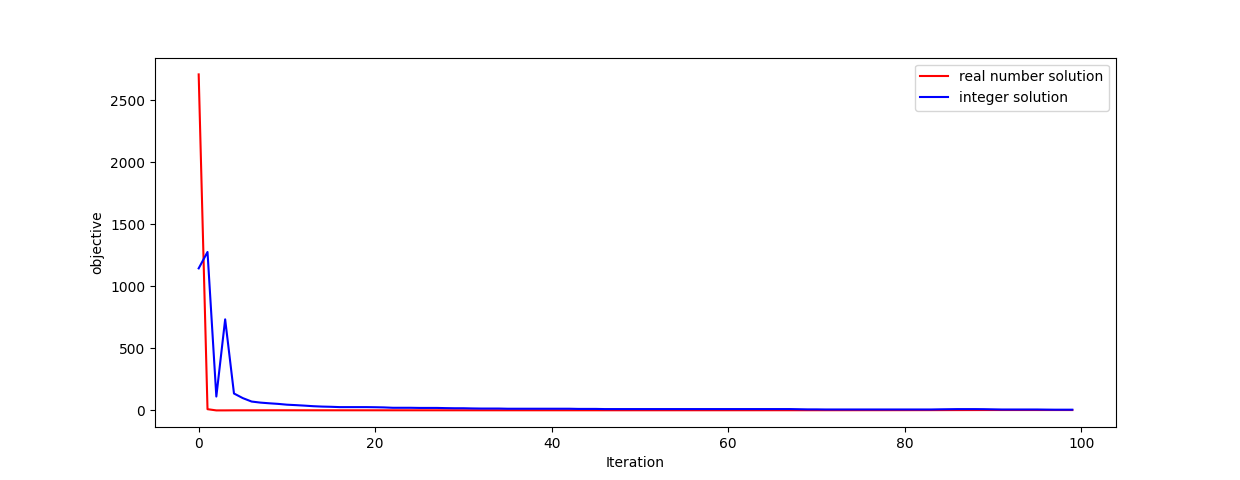
Following the case of financial product marketing, we have nearly 1.1 hundred of million users and 21 equity fund owners each day. We show the results of our algorithm for solving this real-world large scale problem in Figure 5. We first show the objectives w.r.t. real number solution and integer solution and their APD as our algorithm converges. It shows that the objective gap between integer solution and real number solution is large at the first few round of iterations but converges to 0.00231 as the real number solutions approximate to either 0 or 1. We also show the MAPD of equality constraint that the violation being consistently optimized up to 0.00081.



5.2.2. Deployment and Online Results
We first describe the deployment of our distributed solver, then present the online results. We demonstrate the overall workflow in Figure 4. We have fund owners and Alipay users. We allow fund owners to config parameters such as inventory of supply and desired population of users. The Alipay notification marketing system maintains the overall workflow. Note that the overall decision making is data-driven based, i.e., it relies on machine learning components to predict the scores such as the probability of purchase . The system first requests the “ML scoring” component to retrieve the scores (i.e., coefficients of our assignment problem) for final decision making. The “ML scoring” component requests “Feature store” to access the necessary features. After returning the scores back to “Notification system”, the system sends such coefficients to our distributed solver (see details in Figure 1). After solving the assignment problem, the solver returns the decisions and finally completes the notification to Alipay users. We further have monitors to record the quality of our solutions.
The fund owners prepare the inventory and configure the numbers each day. They may also periodically adjust the desired population . Given those parameters, we solve the problem each day. Note that the lower objective value the better, and the lower mean equality violation (MAPD) the better. We report the average relative improvements w.r.t. the quality of our solution compared with a heuristic approach in 7 days in Table 7.
| Metrics | Our solver |
|---|---|
| Objective | 14.20% improvement |
| Mean Equality Violation | +7.20% improvement |
6. Conclusions
We introduced the formulation for a class of assignment problems. The formulation supports nonlinear objective, convex per-item constraints, and feature-owner cross constraints. It is more general than GAP, and covers many real-world business problems. In the era of big data, there are scenarios when solving such problems with billions of decision variables is essential to business. To achieve such scale, we adapted the Bregman ADMM framework to our problem and obtained a distributed algorithm. In experiments, we specified the full Bregman ADMM construction for two example problems, with quadratic and logarithmic objectives, respectively. Using synthetic data, we showed the correctness of our implementation, and scaled the solver to problems of one billion decision variables. We deploy our distributed solver to production and show its application to business decision making in an internet scale.
References
- (1)
- Avella et al. (2013) Pasquale Avella, Maurizio Boccia, and Igor Vasilyev. 2013. A branch-and-cut algorithm for the multilevel generalized assignment problem. IEEE Access 1 (2013), 475–479.
- Bertsekas and Tsitsiklis (1989) Dimitri P Bertsekas and John N Tsitsiklis. 1989. Parallel and distributed computation: numerical methods. Vol. 23. Prentice hall Englewood Cliffs, NJ.
- Boyd et al. (2011) Stephen Boyd, Neal Parikh, and Eric Chu. 2011. Distributed optimization and statistical learning via the alternating direction method of multipliers. Now Publishers Inc.
- Cattrysse and Van Wassenhove (1992) Dirk G Cattrysse and Luk N Van Wassenhove. 1992. A survey of algorithms for the generalized assignment problem. European journal of operational research 60, 3 (1992), 260–272.
- Ceselli and Righini (2006) Alberto Ceselli and Giovanni Righini. 2006. A branch-and-price algorithm for the multilevel generalized assignment problem. Operations research 54, 6 (2006), 1172–1184.
- Cheng et al. (2020) Dawei Cheng, Zhibin Niu, and Yiyi Zhang. 2020. Contagious chain risk rating for networked-guarantee loans. In Proceedings of the 26th ACM SIGKDD International Conference on Knowledge Discovery & Data Mining. 2715–2723.
- Chu and Beasley (1997) Paul C Chu and John E Beasley. 1997. A genetic algorithm for the generalised assignment problem. Computers & Operations Research 24, 1 (1997), 17–23.
- Deng et al. (2017) Wei Deng, Ming-Jun Lai, Zhimin Peng, and Wotao Yin. 2017. Parallel multi-block ADMM with O (1/k) convergence. Journal of Scientific Computing 71, 2 (2017), 712–736.
- Deng and Yin (2016) Wei Deng and Wotao Yin. 2016. On the global and linear convergence of the generalized alternating direction method of multipliers. Journal of Scientific Computing 66, 3 (2016), 889–916.
- Feltl and Raidl (2004) Harald Feltl and Günther R Raidl. 2004. An improved hybrid genetic algorithm for the generalized assignment problem. In Proceedings of the 2004 ACM symposium on Applied computing. 990–995.
- Fisher et al. (1986) Marshall L Fisher, Ramchandran Jaikumar, and Luk N Van Wassenhove. 1986. A multiplier adjustment method for the generalized assignment problem. Management science 32, 9 (1986), 1095–1103.
- Gavish and Pirkul (1991) Bezalel Gavish and Hasan Pirkul. 1991. Algorithms for the multi-resource generalized assignment problem. Management science 37, 6 (1991), 695–713.
- He and Yuan (2012) Bingsheng He and Xiaoming Yuan. 2012. On the O(1/n) convergence rate of the Douglas–Rachford alternating direction method. SIAM J. Numer. Anal. 50, 2 (2012), 700–709.
- Hong and Luo (2017) Mingyi Hong and Zhi-Quan Luo. 2017. On the linear convergence of the alternating direction method of multipliers. Mathematical Programming 162, 1-2 (2017), 165–199.
- Jörnsten and Näsberg (1986) Kurt Jörnsten and Mikael Näsberg. 1986. A new Lagrangian relaxation approach to the generalized assignment problem. European Journal of Operational Research 27, 3 (1986), 313–323.
- Karakoulas (2004) Grigoris Karakoulas. 2004. Empirical validation of retail credit-scoring models. RMA JOURNAL 87 (2004), 56–60.
- Krumke and Thielen (2013) Sven O Krumke and Clemens Thielen. 2013. The generalized assignment problem with minimum quantities. European Journal of Operational Research 228, 1 (2013), 46–55.
- Liu et al. (2019a) Qinghua Liu, Xinyue Shen, and Yuantao Gu. 2019a. Linearized admm for nonconvex nonsmooth optimization with convergence analysis. IEEE Access 7 (2019), 76131–76144.
- Liu et al. (2019b) Ziqi Liu, Dong Wang, Qianyu Yu, Zhiqiang Zhang, Yue Shen, Jian Ma, Wenliang Zhong, Jinjie Gu, Jun Zhou, Shuang Yang, et al. 2019b. Graph representation learning for merchant incentive optimization in mobile payment marketing. In Proceedings of the 28th ACM International Conference on Information and Knowledge Management. 2577–2584.
- Lourenço and Serra (1998) H Ramalhinho Lourenço and Daniel Serra. 1998. Adaptive approach heuristics for the generalized assignment problem. DEE-UPF, Economic Working paper Series 288 (1998).
- Martello (1990) Silvano Martello. 1990. Knapsack problems: algorithms and computer implementations. Wiley-Interscience series in discrete mathematics and optimiza tion (1990).
- Martello et al. (1981) Silvano Martello et al. 1981. An algorithm for the generalized assignment problem. (1981).
- Osman (1995) Ibrahim H Osman. 1995. Heuristics for the generalised assignment problem: simulated annealing and tabu search approaches. Operations-Research-Spektrum 17, 4 (1995), 211–225.
- Parikh and Boyd (2014) Neal Parikh and Stephen Boyd. 2014. Proximal algorithms. Foundations and Trends in optimization 1, 3 (2014), 127–239.
- Ross and Soland (1975) G Terry Ross and Richard M Soland. 1975. A branch and bound algorithm for the generalized assignment problem. Mathematical programming 8, 1 (1975), 91–103.
- Savelsbergh (1997) Martin Savelsbergh. 1997. A branch-and-price algorithm for the generalized assignment problem. Operations research 45, 6 (1997), 831–841.
- Takapoui et al. (2020) Reza Takapoui, Nicholas Moehle, Stephen Boyd, and Alberto Bemporad. 2020. A simple effective heuristic for embedded mixed-integer quadratic programming. Internat. J. Control 93, 1 (2020), 2–12.
- Wächter and Biegler (2006) Andreas Wächter and Lorenz T Biegler. 2006. On the implementation of an interior-point filter line-search algorithm for large-scale nonlinear programming. Mathematical programming 106, 1 (2006), 25–57.
- Wang and Banerjee (2013) Huahua Wang and Arindam Banerjee. 2013. Bregman alternating direction method of multipliers. arXiv preprint arXiv:1306.3203 (2013).
- Wang et al. (2016) Yijun Wang, Le Wu, Zongda Wu, Enhong Chen, and Qi Liu. 2016. Selecting valuable customers for merchants in e-commerce platforms. In 2016 IEEE 16th International Conference on Data Mining (ICDM). IEEE, 1281–1286.
- Xiong et al. (2017) Sheng Xiong, Yuqi Yang, and Kaizhan Huai. 2017. A new model of generalized assignment problem and its method. In 2017 IEEE 2nd Advanced Information Technology, Electronic and Automation Control Conference (IAEAC). IEEE, 2379–2384.
- Yu et al. (2021) Li Yu, Zhengwei Wu, Tianchi Cai, Ziqi Liu, Zhiqiang Zhang, Lihong Gu, Xiaodong Zeng, and Jinjie Gu. 2021. Joint Incentive Optimization of Customer and Merchant in Mobile Payment Marketing. In Proceedings of the AAAI Conference on Artificial Intelligence, Vol. 35. 15000–15007.
- Zhou et al. (2021) Jun Zhou, Yang Bao, Hua Wu, and Zhigang Hua. 2021. AntOpt: A Multi-functional Large-scale Decision Optimization Platform. In Proceedings of the 30th ACM International Conference on Information & Knowledge Management. 4833–4837.