Gravitational decoherence by the apparatus in the quantum-gravity induced entanglement of masses

The theory of General Relativity (GR) is one of the most well-tested theories of physics, successfully passing a number fundamental tests (will2014confrontation), with its latest success being the observation of gravitational waves (LIGOScientific:2016aoc). However, at short-distance scales and early times, where quantum effects start playing an important role, GR breaks down (Hawking:1973uf), and a quantum theory of gravity is needed. There are several candidate quantum gravity (QG) theories, such as string theory (Bjerrum-Bohr:2004qcf) and loop quantum gravity (Thiemann:2006cf), but despite theoretical progress, the connection with experiments has remained elusive (amelino2013quantum).

Albeit the quantization of gravity is an often-used tool in theoretical physics, forming the backbone of candidate quantum-gravity theories, thus far, there is no definitive experimental evidence in support of the quantum nature of gravity. The reason is simple – the weakness of the gravitational force makes direct detection of gravitons a formidable challenge, a situation which will likely persist in the foreseeable future (Dyson:2013hbl). On the other hand, indirect tests of the quantum nature of gravity (with the first discussions dating back to Feynman (feynman:1957)) have in recent years become a real prospect with the advances in precision sensing and metrology, opening the possibility of probing genuine quantum features of gravity with tabletop experiments.

In 2017 a simple experiment for a definitive test of the quantum nature of gravity was proposed in (Bose:2017nin), along with its relevant background and feasibility studies (for a related work see (Marletto:2017kzi)). The idea exploits the quantum-gravity-induced entanglement of masses (QGEM) to discern between all classical models of gravity from the quantum one ¹¹ 1 When talking about a theory of quantum gravity, we assume an effective quantum field theory where a massless spin-$2$ graviton acts as a force carrier for the gravitational force, and which behaves well at low energies (Donoghue:1994dn).. Two nearby masses, each delicately prepared in a spatial superposition, are placed close enough that that their mutual gravitational interaction can generate entanglement, but still far enough that all other interactions are strongly suppressed. The generated entanglement can be detected by measuring quantum correlations between the two masses, a genuinely quantum effect with no classical analogue, and, if detected, would provide the first definite evidence for the quantization of the gravitational field.

The argument for the entanglement-based test of the quantization of gravity can be summarized as follows. To generate matter-matter entanglement one requires a quantum interaction coupling the two systems; the quantum matter-matter gravitational interaction (which in the non-relativistic regime is the operator-valued Newtonian potential) corresponds to the shift of the energy of the gravitational field, hence requiring the gravitational field itself to be a quantum operator, ruling out the possibility of a (real-valued) classical gravitational field (Bose:2022uxe). Formally, entanglement between two quantum states cannot be increased with local operations and classical communications (LOCC) (Bennett:1996gf), as would be the case with a classical gravitational field, and hence, if gravitationally induced entanglement is detected, the gravitational interaction must be ostensibly quantum in nature. This argument has been discussed in detail within the context of perturbative quantum gravity (Marshman:2019sne; Bose:2022uxe), the path-integral approach (Christodoulou2), and the Arnowitt-Desse-Meissner (ADM) formalism (Danielson).

To discern the spin character of the graviton it is however not sufficient to consider non-relativistic matter-matter interactions but one needs to devise an experiment where gravity couples relativistic fields. One promising possibility is to probe the quantum light-bending interaction between a heavy mass and photons in a cavity where the degree of the generated entanglement can be used to distinguish between spin $2$ and spin $0$ mediators of the gravitational field Biswas:2022qto. Another option is to consider matter-matter interactions beyond the static limit where the post-Newtonian corrections encode the spin character (Bose:2022uxe).

In this paper we consider the conceptually simple scheme with gravitationally coupled harmonic oscillators and quantify the generated entanglement up to the second post Newtonian contribution.

In order to realise such an experiment one has to overcome are many challenges, such as the preparation of the initial state (Marshman:2021wyk; Margalit:2020qcy; Zhou:2022frl; Marshman:2021wyk), the isolation of the system (vandeKamp:2020rqh; Chevalier:2020uvv; Barker:2022mdz) and the reduction of noise (Toros:2020dbf). The shielding of the system from spurious interactions will never be completely perfect, and the matter systems will loose their coherence due to interaction with the environment. Methods for battling the decoherence have been proposed previously (Schut:2021svd; Tilly:2021qef; Pedrnales), and many sources of decoherence have been discussed, such as in (Toros:2020krn; Rijavec:2020qxd; Torrieri:2022znj).

There is however one source of inherent decoherence which has thus far not been analyzed in detail. In order to witness the generated entanglement we require the presence of nearby experimental apparatus; while electromagnetic couplings between a neutral mass (the light system) and the lab equipment (the heavy system) can be suppressed with appropriate shielding, their mutual gravitational interaction is unavoidable, and scales unfavourably with the mass of the laboratory apparatus. The heavy laboratory equipment, which can be modelled quantum mechanically, can entangle with the two neutral masses, thus providing an unavoidable source of gravitational decoherence.

When we talk about the ‘apparatus’ or ‘laboratory equipment’ we refer to anything close to the experiment that can be quantum, such as the current carrying wires in the Stern-Gerlach setup (Margalit:2020qcy; Marshman:2021wyk; Zhou:2022jug; Zhou:2022frl). We call any such source the ‘heavy mass’, in this paper we consider two heavy systems A and B with mass $m_{A}=m_{B}=M$. The aim of this paper is to analyze this gravity-induced decoherence in presence of the heavy masses in a model independent fashion, and to quantify the attenuation of the entanglement between the two light quantum masses.

In this paper we will study decoherence with an entanglement measure, the concurrence, which quantifies how much the laboratory equipment and the test masses are entangled. An often-used approach to analyze decoherence is also to trace out the ‘environment’ system and find the remaining entanglement between the test masses. We briefly discuss this latter approach in Sec. VI, but when we talk about ‘the decoherence’ we refer to the entanglement between the apparatus and the test masses.

First, we will introduce the setup consisting of two heavy quantum harmonic oscillators (representing the laboratory apparatus) and two light quantum harmonic oscillators (representing the two test masses), and introduce all the relevant interactions (Sec. II). We will then discuss how to calculate the entanglement using concurrence between the two subsystems that are coupled by the quantized gravitational field within perturbative quantum gravity (Sec. III). Then we discuss the induced decoherence on the two light systems in the static limit (Sec. IV) as well as in the higher order momentum corrections by considering the light systems up to the second post Newtonian contribution (Sec. V). We find the allowed parameter space where the entanglement between the light systems dominates the decoherence (Sec. VI) and we will conclude with a discussion of the results (Sec. VII).

Let us consider four massive systems, denoted by $a,b,A,B$ with light masses $m_{a},\penalty\ m_{b}$ and heavy masses $m_{A},\penalty\ m_{B}$, respectively. We wish to understand the entanglement of $m_{a},\penalty\ m_{b}$ via the quantum nature of gravity, while $m_{A},\penalty\ m_{B}$ would be responsible for gravitationally decohering the light masses. These massive systems are placed in harmonic traps located at $\pm\frac{d}{2}$ for systems $a,b$ and located at $\pm\frac{D}{2}$ for systems $A,\penalty\ B$. We will assume $D>d$.

Taking the harmonic oscillators to be well-localized, we obtain:

	$\displaystyle\hat{x}_{a}$	$\displaystyle=-\frac{d}{2}+\delta\hat{x}_{a}\,,\quad\mbox{}\quad\,\,\,\hat{x}_{b}=\frac{d}{2}+\delta\hat{x}_{b}\,,$		(1)
	$\displaystyle\hat{x}_{A}$	$\displaystyle=-\frac{D}{2}+\delta\hat{x}_{A}\,,\quad\mbox{}\quad\hat{x}_{B}=\frac{D}{2}+\delta\hat{x}_{B}\,,$		(2)

with $\hat{x}_{i}$ and $\delta\hat{x}_{i}$ the position operators and small equilibrium displacement for system $i=a,\penalty\ b,\penalty\ A,\penalty\ B$. We will further assume that all the masses are neutral to minimize the electromagnetic interactions. Although there will be dipolar interactions between all these systems; the Casimir induced dipole-dipole interactions between the two systems $a,\penalty\ A$ and $b,\penalty\ B$ can be minimised by placing a conducting plate, while the Casimir interaction between a light and a heavy system can be minimised by giving some hierarchy between $D$ and $d$. The Hamiltonian for the matter systems is given by:

$$\hat{H}_{\text{m}}=\sum_{i=a,b,A,B}\frac{\hat{p}_{i}^{2}}{2m_{i}}+\frac{m_{i}\omega_{i}^{2}}{2}\delta\hat{x}_{i}^{2}\,,$$

(3)

with $\hat{p}_{i}$ and $\omega_{i}$ the conjugate momenta and the trap’s harmonic frequency for system $i$, respectively. The basis is chosen such that the matter systems are uncoupled which will simplify our computations ²² 2 As an initial system we can choose a Hamiltonian where there is a coupling between systems $a$ ($b$) and $A$ ($B$): $\displaystyle\hat{H}_{\text{m}}=\sum_{i=1,2,3,4}\frac{\hat{p}_{i}^{\prime 2}}{2m_{i}}$ $\displaystyle+\frac{k_{0}}{2}(\delta\hat{x}_{1}^{2}+\delta\hat{x}_{2}^{2})+\frac{k_{1}}{2}(\delta\hat{x}_{1}-\delta\hat{x}_{2})^{2}$ $\displaystyle+\frac{k_{2}}{2}(\delta\hat{x}_{3}^{2}+\delta\hat{x}_{4}^{2})+\frac{k_{3}}{2}(\delta\hat{x}_{3}-\delta\hat{x}_{4})^{2}\,.$ (4) Then there exists a unitary transformation such that the Hamiltonian becomes decoupled. After the transformation the matter Hamiltonian can be written as $$\hat{H}_{\text{m}}=\hat{H}_{a}+\hat{H}_{b}+\hat{H}_{A}+\hat{H}_{B}\,.$$ (5) with $\hat{H}_{i}=\frac{\hat{p}_{i}^{2}}{2m_{i}}+\frac{1}{2}m_{i}\omega_{i}^{2}\hat{x}_{i}^{2}$, and with $\omega_{a(b)}^{2}=k_{0(2)}/m_{a(b)}$, $\omega_{A(B)}^{2}=[k_{0(2)}+2k_{1(3)}]/m_{A(B)}$. The change of basis is given as: $$\hat{x}_{a(b)}=[\hat{x}_{1(3)}+\hat{x}_{2(4)}]/\sqrt{2},\quad\mbox{}\quad\hat{x}_{A(B)}=[\hat{x}_{1(3)}-\hat{x}_{2(4)}]/\sqrt{2}\,.$$ . The mode operators for the harmonic oscillator systems are given by:

$\displaystyle\delta\hat{x}_{j}=\sqrt{\frac{\hbar}{2m_{j}\omega_{j}}}(j+j^{\dagger})\,,\,\,\hat{p}_{j}=i\sqrt{\frac{\hbar m_{j}\omega_{j}}{2}}(j-j^{\dagger})\,,$

(6)

with $j=a,b,A,B$, and the operators satisfying the usual commutation relations ³³ 3 These commutation relations are: $\displaystyle[a,a]=[b,b]=[A,A]=[B,B]=0$ $\displaystyle[a^{\dagger},a^{\dagger}]=[b^{\dagger},b^{\dagger}]=[A^{\dagger},A^{\dagger}]=[B^{\dagger},B^{\dagger}]=0$ $\displaystyle[a,a^{\dagger}]=[b,b^{\dagger}]=[A,A^{\dagger}]=[B,B^{\dagger}]=1\,.$ . Thus the Hamiltonian can be written as:

$$\hat{H}_{\text{m}}=\hbar\omega_{a}\hat{a}^{\dagger}\hat{a}+\hbar\omega_{b}\hat{b}^{\dagger}\hat{b}+\hbar\omega_{A}\hat{A}^{\dagger}\hat{A}+\hbar\omega_{B}\hat{B}^{\dagger}\hat{B}\,.$$

(7)

We now introduce a gravitational field and study the interaction Hamiltonian $\hat{H}_{\text{int}}$ between the gravitational and matter fields.

We work in linearized gravity where the metric is given by $g_{\mu\nu}=\eta_{\mu\nu}+h_{\mu\nu}$, with $\eta_{\mu\nu}$ the flat Minkowski background with signature $(-,+,+,+)$ and with $h_{\mu\nu}$ a perturbation which is small in magnitude around the Minkowski background. The metric fluctuations are then promoted to quantum operators:

$\displaystyle\hat{h}_{\mu\nu}=\mathcal{A}\int\differential[3]{k}\sqrt{\frac{\hbar}{2\omega_{k}(2\pi)^{3}}}\left(\hat{P}_{\mu\nu}^{\dagger}(\vec{k})e^{-i\vec{k}\vec{r}}+\text{H.c.}\right),$

(8)

with $\mathcal{A}=\sqrt{16\pi G/c^{2}}$, and where $\hat{P}_{\mu\nu}$ and $\hat{P}_{\mu\nu}^{\dagger}$ denote the graviton annihilation and creation operators, respectively, and satisfy the following commutation relations (Gupta-1952):

$\displaystyle[\hat{P}_{\mu\nu}(\vec{k}),\hat{P}_{\rho\sigma}^{\dagger}(\vec{k}^{\prime})]=(\eta_{\mu\rho}\eta_{\nu\sigma}+\eta_{\mu\sigma}\eta_{\nu\rho})\delta(\vec{k}-\vec{k}^{\prime})\,.$

(9)

In the weak field regime we can decompose the metric fluctuation operator into two modes: the spin-$2$ mode $\gamma_{\mu\nu}$ and the spin-0 mode $\gamma\equiv\eta_{\mu\nu}\gamma^{\mu\nu}$ (Gupta-1952) ⁴⁴ 4 These two modes can be treated independently. $\gamma_{\mu\nu}$ is sometimes called the trace-reversed metric since $h=-\gamma$. . Such that: $\hat{h}_{\mu\nu}=\hat{\gamma}_{\mu\nu}-\frac{1}{2}\eta_{\mu\nu}\hat{\gamma}\,.$ Consequently the spin-$2$ and spin-$0$ decomposed parts of the graviton can be promoted to operators as well, and they are given in terms of the graviton creation- and annihilation operators (Gupta-1952):

	$\displaystyle\hat{\gamma}_{\mu\nu}=\mathcal{A}\int\differential[3]{k}\sqrt{\frac{\hbar}{2\omega_{k}(2\pi)^{3}}}\left(\hat{P}_{\mu\nu}^{\dagger}(\vec{k})e^{-i\vec{k}\vec{r}}+\text{H.c.}\right),$		(10)
	$\displaystyle\hat{\gamma}=2\mathcal{A}\int\differential[3]{k}\sqrt{\frac{\hbar}{2\omega_{k}(2\pi)^{3}}}\left(\hat{P}^{\dagger}(\vec{k})e^{-i\vec{k}\vec{r}}+\text{H.c.}\right),$		(11)

satisfying the commutation relations in Eq. (9) ⁵⁵ 5 Following Eq. (9) and the definition $\gamma\equiv\eta_{\mu\nu}\gamma^{\mu\nu}$, the additional commutation relation is: $\displaystyle[\hat{P}(\vec{k}),\hat{P}^{\dagger}(\vec{k}^{\prime})]=-\delta(\vec{k}-\vec{k}^{\prime})\,.$ (12) . The gravity Hamiltonian can then be written in terms of graviton creation and annihilation operators (Gupta-1952). Now that both the matter and graviton systems have been introduced, we continue by studying their interaction and in the next section the consequential entanglement generation. The interaction term is given by the graviton coupling to the stress-energy tensor $\hat{T}_{\mu\nu}$ (which specifies the matter system contents):

$$\hat{H}_{\text{int}}=-\frac{1}{2}\int\differential[3]{r}\hat{h}^{\mu\nu}(\vec{r})\hat{T}_{\mu\nu}(\vec{r})\,.$$

(13)

We consider the two harmonically trapped particles $a,b$ to be moving along the $x$-axis, and the two heavy systems $A,B$ to be static. The systems $A,B$ are taken to be static because we consider these systems to be the very massive systems such that their motion remains negligible when perturbed by the two light systems. The four systems thus generate the following currents:

	$\displaystyle\hat{T}_{00}(\vec{r})\equiv\sum_{n=a,b,A,B}m_{n}c^{2}\delta(\vec{r}-\hat{\vec{r}}_{n})\,,$		(14)
	$\displaystyle\hat{T}_{ij}(\vec{r})\equiv\sum_{n=a,b}\frac{\hat{p}_{n,i}\hat{p}_{n,j}}{E/c^{2}}\delta(\vec{r}-\hat{\vec{r}}_{n})\,,$		(15)

with the position of the matter systems $\hat{r}_{n}=(\hat{x}_{n},0,0)$, with the momentum $\hat{p}_{\mu}=(-E/c,\vec{p})$, energy $E=\sqrt{\vec{p}^{2}c^{2}+m^{2}c^{4}}$, and with $i,\penalty\ j=1,2,3$.

Since we specified the movement of the oscillators $a,b$ to be along the $x$-axis, the only non-zero $\hat{T}_{\mu\nu}$-components are $\hat{T}_{01}$, $\hat{T}_{10}$ and $\hat{T}_{11}$. Therefore, the only relevant $\hat{h}_{\mu\nu}$ components in the coupling are $\hat{h}_{00}=\hat{\gamma}_{00}+\frac{1}{2}\hat{\gamma}$, $\hat{h}_{01}=\hat{h}_{10}=\hat{\gamma}_{01}$ and $\hat{h}_{11}=\hat{\gamma}_{11}-\frac{1}{2}\hat{\gamma}$. Writing the interaction Hamiltonian in terms of the decomposed metric perturbation, while exploiting the symmetries $\hat{T}_{01}=\hat{T}_{10}$ and $\hat{\gamma}_{01}=\hat{\gamma}_{10}$, gives:

	$\displaystyle\hat{H}_{\text{int}}$	$\displaystyle=\int\differential[3]{r}\bigg(\frac{1}{2}[\hat{\gamma}_{00}(\vec{r})+\frac{1}{2}\hat{\gamma}(\vec{r})]\,\hat{T}_{00}(\vec{r})$
		$\displaystyle+\frac{1}{2}[\hat{\gamma}_{11}(\vec{r})-\frac{1}{2}\hat{\gamma}(\vec{r})]\,\hat{T}_{11}(\vec{r})+\hat{\gamma}_{10}(\vec{r})\,\hat{T}_{10}(\vec{r})\bigg).$		(16)

As explained in Ref. (Bose:2022uxe), the energy shift in the graviton vacuum due to the above interaction can only induce entanglement when the gravitational field is quantized, with $h_{\mu\nu}$ or equivalently $\gamma_{\mu\nu},\penalty\ \gamma$. This can be formalized using the Local Operations and Classical Communication (LOCC) principle, which states that a LOCC channel (such is the case for a classical real valued gravitational field) cannot increase the entanglement between the two systems. Only Quantum Communication can increase entanglement between the systems (Bose:2022uxe). The graviton here acts as a quantum communicator between the two systems, and is therefore able to induce a coupling that entangles previously unentangled oscillators. This entanglement and decoherence are studied in the next sections.

We assume that initially the quantum matter systems are in the ground state (denoted by $\ket{0}_{i}$, with $i$ specifying the system $i=a,\penalty\ b,\penalty\ A,\penalty\ B$):

$$\ket{\psi_i}=\ket{0}_{a}\ket{0}_{b}\ket{0}_{A}\ket{0}_{B}\,.$$

(17)

Since gravity will couple all the systems, it will induce interaction between the heavy and light oscillators, $\hat{H}_{hl}$ (which is presented in Eqs. (37) and (63)). As a result of this interaction the final state will evolve to: ⁶⁶ 6 Here we have left out the subscripts on the kets to ease the notation. In the remainder of the paper the order of the the states is always $a,\penalty\ b,\penalty\ A,\penalty\ B$.

$$\ket{\psi_f}=\frac{1}{\sqrt{\mathcal{N}}}\sum_{\begin{subarray}{c}n_{a},n_{b}\\ n_{A},n_{B}\end{subarray}}C_{n_{a}n_{b}n_{A}n_{B}}\ket{n_a}\ket{n_b}\ket{n_A}\ket{n_B}\,.$$

(18)

The number states are denoted by $\ket{n_i}$, and the normalisation is given by $\mathcal{N}=\sum_{n_{a},n_{b}\\ n_{A},n_{B}}\absolutevalue{C_{n_a n_b n_A n_B}}^{2}$. The interaction is scaled by a bookkeeping parameter $\lambda$.

In first order perturbation theory the coefficients for the final wavefunction are given by:

$$C_{n_{a}n_{b}n_{A}n_{B}}=\lambda\frac{\bra{n_a}\bra{n_b}\bra{n_A}\bra{n_B}\hat{H}_{hl}\ket{0}\ket{0}\ket{0}\ket{0}}{\sum_{i=a,b,A,B}(E_{0_{i}}-E_{n_{i}})}\,,$$

(19)

for the perturbed states, and $C_{0000}=1$ for the unperturbed state. In the above equation $E_{0_{i}}$ is the ground-state energy and $E_{n_{i}}$ denotes the $n$th excited state energy, for system $i=a,b,A,B$.

At this point it is important to take a note that $\hat{H}_{hl}$ is a quantum operator. If it were classical, so not operator-valued, then for any perturbed coefficients $C_{n_{a}n_{b}n_{A}n_{B}}=0$ due to the orthogonality of the states, thus the final wavefunction would be $\ket{\psi_f}=\ket{0}\ket{0}\ket{0}\ket{0}$, the initial wavefunction. No entanglement can be generated in an initially unentangled system from a classical interaction. Since we are working in the framework of perturbative quantum field theory of gravity we expect an entanglement, which will be quantified by the concurrence of a biparte system, between the subsystems $1$ and $2$ (see below for the choice of the subsystems 1 and 2):

$$\mathcal{C}\equiv\sqrt{2-2\Tr(\rho_1^2)}\,,$$

(20)

where $\rho_{1}=\Tr_{2}(\rho)$ is the partial density matrix found by tracing out subsystem $2$ in the full density matrix $\rho=\ket{\psi_f}\bra{\psi_f}$. The larger the concurrence, the more strongly entangled the subsystems are, where a maximally entangled state gives the value $\sqrt{2}$ and an unentangled state gives the value $0$ ⁷⁷ 7 The concurrence can be related to the maybe better-known and more widely applicable von Neumann entropy via a simple relation (Wootters:1997id)..

The use of concurrence is limited to biparte systems though. As we are interested in the decoherence of the systems $a,\penalty\ b$ due to their coupling to the more massive systems $A,\penalty\ B$, we choose the bipartition such that subsystem $1$ consists of the light oscillators $a,\penalty\ b$ and subsystem $2$ consists of the heavy oscillators $A,\penalty\ B$. Since the entanglement and decoherence are two sides of the same coin, by studying the concurrence for this bipartition we gain information about the effects of the apparatus (the heavy oscillators) on the coherence of the QGEM experiment (the two light particles). For the light-heavy bipartition, the partial density matrix for the light system is

$$\rho_{1}=\frac{1}{\mathcal{N}}\sum_{\begin{subarray}{c}n_{a},n_{b},N_{a},\\ N_{b},n_{A},n_{B}\end{subarray}}C_{n_{a}n_{b}n_{A}n_{B}}C^{*}_{N_{a}N_{b}n_{A}n_{B}}\ket{n_a \, n_b}\bra{N_a \, N_b}$$

(21)

using the notation $\ket{n_a \, n_b}=\ket{n_a}\ket{n_b}$. Inserting this expression into Eq. (20), the heavy-light concurrence, denoted $\mathcal{C}_{\text{hl}}$, can be expressed in terms of the coefficients $C$ defined in Eq. (19):

	$\displaystyle\mathcal{C}_{\text{hl}}\equiv\bigg[2-\frac{2}{\mathcal{N}^{2}}$	$\displaystyle\sum_{\begin{subarray}{c}n_{a},N_{a},n_{b},N_{b}\\ n_{A},n_{B},N_{A},N_{B}\end{subarray}}C_{n_{a}n_{b}n_{A}n_{B}}C^{*}_{N_{a}N_{b}n_{A}n_{B}}$
		$\displaystyle\hskip 19.91692pt\crossproduct C_{n_{a}n_{b}N_{A}N_{B}}C^{*}_{N_{a}N_{b}N_{A}N_{B}}\bigg]^{1/2}.$		(22)

Finding all the relevant expressions of the coefficients in Eq. (19) would result in the quantification of decoherence/entanglement at first order in the perturbation theory. For this we need to find the interaction Hamiltonian between the heavy and light system, $\hat{H}_{\text{hl}}$, which is generated by the exchange of the virtual graviton (see below the derivation with the result in Eq. (37)).

The interaction between gravity and matter is given in Eq. (II), from which we can compute the shift in energy to the graviton vacuum at second order in perturbation theory ⁸⁸ 8 The first order term corresponding to the emission/absorption of a graviton is given by $\bra{0}\hat{H}_{\text{int}}\ket{0}$. This contribution vanishes since $\hat{H}_{\text{int}}$ depends linearly on the graviton creation and annihilation operators, and $\hat{P}\ket{0}=\hat{P}_{\mu\nu}\ket{0}=0$, $\bra{0}\hat{P}^{\dagger}=\bra{0}\hat{P}_{\mu\nu}^{\dagger}=0$. In the second order term (corresponding to the exchange of a virtual graviton) $\bra{0}\hat{H}_{\text{int}}|\vec{k}\rangle$ is quadratically dependent on the creation an annihilation operators. Using the operator commutation rules shows that this contribution is non-vanishing. :

$$\Delta\hat{H}_{g}\equiv\int\differential[3]{k}\frac{\bra{0}\hat{H}_{\text{int}}|\vec{k}\rangle\langle\vec{k}|\hat{H}_{\text{int}}\ket{0}}{E_{0}-E_{k}}\,,$$

(23)

with $E_{0}$ the energy of the vacuum state, and $E_{k}=E_{0}+\hbar\omega_{k}$ the energy of of the one-particle state $|\vec{k}\rangle$ representing the intermediate graviton, which is created from the vacuum with the graviton creation operators. The collection of normalized projectors $|\vec{k}\rangle\langle\vec{k}|$ is given by:

	$\displaystyle|\vec{k}\rangle\langle\vec{k}|$	$\displaystyle=\frac{1}{2}P^{\dagger}_{00}(\vec{k})\ket{0}\bra{0}P_{00}(\vec{k})+\frac{1}{2}P^{\dagger}_{11}(\vec{k})\ket{0}\bra{0}P_{11}(\vec{k})$
		$\displaystyle-P^{\dagger}_{01}(\vec{k})\ket{0}\bra{0}P_{01}(\vec{k})-P^{\dagger}(\vec{k})\ket{0}\bra{0}P(\vec{k}).$		(24)

For each projector summed in the above expression we can evaluate $\bra{0}\hat{H}_{\text{int}}|\vec{k}\rangle$, with the interaction given in Eq. (II):

	$\displaystyle\bra{0}\hat{H}_{\text{int}}\hat{P}_{00}(\vec{k})|\vec{0}\rangle$	$\displaystyle=\mathcal{A}\sqrt{\frac{\hbar}{2\omega_{k}}}\hat{T}_{00}(\vec{k})\,,$		(25)
	$\displaystyle\bra{0}\hat{H}_{\text{int}}\hat{P}_{11}(\vec{k})|\vec{0}\rangle$	$\displaystyle=\mathcal{A}\sqrt{\frac{\hbar}{2\omega_{k}}}\hat{T}_{11}(\vec{k})\,,$		(26)
	$\displaystyle\bra{0}\hat{H}_{\text{int}}\hat{P}_{01}(\vec{k})|\vec{0}\rangle$	$\displaystyle=\mathcal{A}\sqrt{\frac{\hbar}{2\omega_{k}}}\hat{T}_{01}(\vec{k})\,,$		(27)
	$\displaystyle\bra{0}\hat{H}_{\text{int}}\hat{P}(\vec{k})|\vec{0}\rangle$	$\displaystyle=\frac{\mathcal{A}}{2}\sqrt{\frac{\hbar}{2\omega_{k}}}\left[\hat{T}_{00}(\vec{k})-\hat{T}_{11}(\vec{k})\right]\,,$		(28)

with $\mathcal{A}\equiv\sqrt{16\pi G/c^{2}}$. $\hat{T}_{\mu\nu}(\vec{k})$ are the stress-energy tensor components in momentum space ⁹⁹ 9 The momentum-space stress-energy tensor components are given by the Fourier transform of the components in position space: $$\hat{T}_{\mu\nu}(\vec{k})=\frac{1}{(2\pi)^{3/2}}\int\differential[]{r}e^{-i\vec{k}\cdot\vec{r}}\hat{T}_{\mu\nu}(\vec{r})\,.$$ (29) , which from Eqs. (14),(15) are found to be:

	$\displaystyle\hat{T}_{00}(\vec{k})$	$\displaystyle=\frac{1}{(2\pi)^{3/2}}\bigg[m_{A}c^{2}e^{-i\vec{k}\cdot\hat{r}_{A}}+m_{B}c^{2}e^{-i\vec{k}\cdot\hat{r}_{B}}$
		$\displaystyle\quad\mbox{}\quad\quad\mbox{}\quad\quad\mbox{}\quad+E_{a}e^{-i\vec{k}\cdot\hat{r}_{a}}+E_{b}e^{-i\vec{k}\cdot\hat{r}_{b}}\bigg],$		(30)
	$\displaystyle\hat{T}_{01}(\vec{k})$	$\displaystyle=-\frac{c}{(2\pi)^{3/2}}\left[\hat{p}_{a}e^{-i\vec{k}\cdot\hat{r}_{a}}+\hat{p}_{b}e^{-i\vec{k}\cdot\hat{r}_{b}}\right],$		(31)
	$\displaystyle\hat{T}_{11}(\vec{k})$	$\displaystyle=\frac{1}{(2\pi)^{3/2}}\left[\frac{\hat{p}_{a}^{2}c^{2}}{E_{a}}e^{-i\vec{k}\cdot\hat{r}_{a}}+\frac{\hat{p}_{b}^{2}c^{2}}{E_{b}}e^{-i\vec{k}\cdot\hat{r}_{b}}\right].$		(32)

Filling in Eqs. (30)-(32) and Eqs. (25)-(28) into Eq. (23) gives an expression for the graviton energy shift from the vacuum, $\Delta\hat{H}_{g}$. This expression can be simplified by performing the integral over $\vec{k}$ ¹⁰¹⁰ 10 This integration is simply $$\int\frac{\differential[3]{k}}{(2\pi)^{3}}\frac{1}{|\vec{k}|^{2}}e^{i\vec{k}\cdot\hat{\vec{r}}}=\frac{1}{4\pi\hat{\vec{r}}}\,,$$ (33) and the expression was rewritten such that $\hat{\vec{r}}=\hat{\vec{x}}_{i}-\hat{\vec{x}}_{j}$. . Furthermore we restrict the movement to the $x$-axis, meaning that $\hat{p}_{i,y}=\hat{p}_{i,z}=0$, $\hat{p}_{i,x}\equiv\hat{p}_{i}$ and $\hat{r}_{i}=(\hat{x}_{i},0,0)$ for $i=a,b,A,B$, to find the expression:

	$\displaystyle\Delta\hat{H}_{g}$	$\displaystyle=-\frac{\mathcal{A}^{2}}{16\pi c^{2}}\Bigg[\frac{m_{A}E_{a}c^{2}+m_{A}\frac{\hat{p}_{a}^{2}c^{4}}{E_{a}}}{\absolutevalue{\hat{x}_A - \hat{x}_a}}$
		$\displaystyle+\frac{m_{A}E_{b}c^{2}+m_{A}\frac{\hat{p}_{b}^{2}c^{4}}{E_{b}}}{\absolutevalue{\hat{x}_{A} - \hat{x}_{b}}}+\frac{m_{A}m_{B}c^{4}}{\absolutevalue{\hat{x}_{A} - \hat{x}_{B}}}$
		$\displaystyle+\frac{E_{a}E_{b}-4\hat{p}_{a}\hat{p}_{b}c^{2}+\hat{p}_{a}^{2}c^{2}\frac{E_{b}}{E_{a}}+\hat{p}_{b}^{2}c^{2}\frac{E_{a}}{E_{b}}+\frac{\hat{p}_{a}^{2}\hat{p}_{b}^{2}c^{4}}{E_{a}E_{b}}}{\absolutevalue{\hat{x}_{a} - \hat{x}_{b}}}$
		$\displaystyle+\frac{m_{B}E_{a}c^{2}+m_{B}\frac{\hat{p}_{a}^{2}c^{4}}{E_{a}}}{\absolutevalue{ \hat{x}_{a} - \hat{x}_{B}}}+\frac{m_{B}E_{b}c^{2}+m_{B}\frac{\hat{p}_{b}^{2}c^{4}}{E_{b}}}{\absolutevalue{ \hat{x}_{b} - \hat{x}_{B}}}\Bigg].$		(34)

Taking $m_{a}=m_{b}=m$ and $m_{A}=m_{B}=M$, and expanding Eq. (34) in powers of $1/c^{2}$ gives the non-relativistic couplings among the $4$ oscillators upto order $1/c^{4}$, and in first order in $G$, the full expression is presented in Eq. (62) ¹¹¹¹ 11 We can reach the classical point particle limit by substituting $\vec{r}\equiv\vec{x_{i}}-\vec{x_{j}}$ with the number-valued distances discussed in Sec. II, the potential becomes: $\displaystyle\Delta H_{g}$ $\displaystyle=-G\bigg[\frac{m^{2}}{d}+\frac{M^{2}}{D}-\frac{8mM}{d^{2}-D^{2}}\bigg]$ $\displaystyle-\frac{G}{c^{2}}\bigg[\frac{3p_{a}^{2}-8p_{a}p_{b}+3p_{b}^{2}}{2d}-\frac{6DM(p_{a}^{2}+p_{b}^{2})}{(d^{2}-D^{2})m}\bigg]$ $\displaystyle-\frac{G}{c^{4}}\bigg[\frac{5p_{a}^{4}-18p_{a}^{2}p_{b}^{2}+5p_{b}^{4}}{8dm^{2}}-\frac{20DM(p_{a}^{4}+p_{b}^{4})}{8(d^{2}-D^{2})m^{3}}\bigg]$ $\displaystyle+\order{\frac{1}{c^6}}\,.$ (35) If the heavy systems are not taken into account, i.e. $M=0$, Eq. (35) reduces to the same expression found in Ref. (Bose:2022uxe) for the interaction between two harmonic oscillators. Furthermore, in the center-of-mass frame, i.e. $p\equiv p_{a}=-p_{b}$, Eq. (35) gives a potential that matches known results for the non-relativistic potential between classical point particles (Grignani:2020ahv; Iwasaki:1971vb; Cristofoli:2019neg)..

In this section we give the expression for the decoherence due to the gravitational interaction between the heavy and light systems. We find the decoherence using an entanglement measure, the concurrence, given in Eq. (III), which quantifies the information of the light system shared with the heavy system. We start by finding the first order interaction terms between the heavy and light systems. We can substitute the expressions (1),(2) for the position operators in terms of their displacements into the Hamiltonian in Eq. (62), and look at the lowest order coupling between the light and heavy matter systems ¹²¹² 12 Since we are considering a bipartite heavy-light system, only the interaction between heavy and light is taken into account to find the decoherence. Any heavy-heavy or light-light interaction can be viewed as ‘self-interaction’ since it only causes entanglement within the subsystem. However, the strength of the light-light entanglement is important to analyse the decoherence effects of the heavy system. Taking into account only the light-light couplings in Eq. (62) and following the same procedure as described in this section, we find the concurrence between the two light oscillators at lowest order to be: $\displaystyle\mathcal{C}_{\text{ll}}$ $\displaystyle=\frac{Gm}{d^{3}\omega_{l}^{2}}+\frac{2Gm}{c^{2}d}\,,$ (36) where we have taken the first order coupling, which consists of a static contribution (from the position operator coupling) and a non-static contribution (from momentum operator coupling), with the momentum contribution being suppressed by $1/c^{2}$. . These can be found by Taylor expanding the small displacements $\delta\hat{x}_{i}$, giving the lowest order interaction terms:

$$\hat{H}_{hl}=16GmM\bigg[\frac{\delta\hat{x}_{a}\delta\hat{x}_{A}+\delta\hat{x}_{b}\delta\hat{x}_{B}}{(D-d)^{3}}+\frac{\delta\hat{x}_{A}\delta\hat{x}_{b}+\delta\hat{x}_{a}\delta\hat{x}_{B}}{(D+d)^{3}}\bigg]$$

(37)

Note that in the above expression there is no coupling between the momentum and the position operators, even though the light system is taken to be non-static. This is because the lowest order coupling is between one heavy position/momentum operator and one light position/momentum operator. The coupling with momentum operators at this order appears as $-4G\hat{p}_{a}\hat{p}_{b}/dc^{2}$, it only gives a coupling between the two light particles instead of the light and heavy subsystems.

We will now use the mode operators in Eq. (6) to write $\hat{H}_{hl}$ in terms of the mode operators $j,j^{\dagger}$ with $j=a,b,A,B$. The resulting Hamiltonian is:

$\displaystyle\hat{H}_{hl}^{\text{op}}=\frac{8G\hbar\sqrt{Mm}}{\sqrt{\omega_{l}\omega_{h}}}\left[\frac{a^{\dagger}A^{\dagger}+b^{\dagger}B^{\dagger}}{(D-d)^{3}}+\frac{a^{\dagger}B^{\dagger}+A^{\dagger}b^{\dagger}}{(D+d)^{3}}\right]\,,$

(38)

where all irrelevant terms (the terms that annihilate the vacuum) have been left out for simplicity. Filling the Hamiltonian in Eq. (38) into Eq. (19), we find the only non-zero coefficients are ¹³¹³ 13 Any terms of the form $\ket{0\, 0 \, n_A \, n_B}$ and $\ket{n_a \, n_b\,0\,0}$ are omitted because they arise from the self-interaction within the light and heavy subsystems, respectively, and are therefore not relevant to our analysis. (where we assumed $\omega_{a}=\omega_{b}=\omega_{l}$ and $\omega_{A}=\omega_{B}=\omega_{h}$ for simplicity, and set $\lambda$ = 1):

	$\displaystyle C_{1010}$	$\displaystyle=C_{0101}=-\frac{\mathfrak{g}_{-}}{\omega_{h}+\omega_{l}}\,,$		(39)
	$\displaystyle C_{0110}$	$\displaystyle=C_{1001}=-\frac{\mathfrak{g}_{+}}{\omega_{h}+\omega_{l}}$		(40)

with

$\displaystyle\mathfrak{g}_{\pm}$

$\displaystyle=\frac{8G}{(D\pm d)^{3}}\frac{\sqrt{mM}}{\sqrt{\omega_{h}\omega_{l}}}\,.$

(41)

The final state given in Eq. (18) (up to the first order in the perturbation theory) is thus given by:

	$\displaystyle\ket{\psi_f}=$	$\displaystyle\frac{1}{\sqrt{\mathcal{N}}}\Big(\ket{0000}-\frac{\mathfrak{g}_{-}}{\omega_{h}+\omega_{l}}\ket{1010}-\frac{\mathfrak{g}_{+}}{\omega_{h}+\omega_{l}}\ket{0110}$
		$\displaystyle-\frac{\mathfrak{g}_{+}}{\omega_{h}+\omega_{l}}\ket{1001}-\frac{\mathfrak{g}_{-}}{\omega_{h}+\omega_{l}}\ket{0101}\Big)\,,$		(42)

with the normalization $\mathcal{N}=1+2(\mathfrak{g}_{-}^{2}+\mathfrak{g}_{+}^{2})/(\omega_{h}+\omega_{l})^{2}$, and using the notation $\ket{n_a}\ket{n_b}\ket{n_A}\ket{n_B}=\ket{n_a\,n_b\,n_A\,n_B}$. The final state is an entangled state between the ground states and first excited states of the light and heavy subsystems. Due to the pair-wise interactions taken here, in each of the perturbed states one heavy and one light system are in the first excited states. Using Eq. (20) the concurrence is found to be:

$$\mathcal{C}_{\text{hl}}^{(1)}=\sqrt{2-2\frac{1+2\frac{(\mathfrak{g}_{-}^{2}+\mathfrak{g}_{+}^{2})^{2}}{\omega^{4}}+8\frac{\mathfrak{g}_{-}^{2}\mathfrak{g}_{+}^{2}}{\omega^{4}}}{\big(1+2\frac{\mathfrak{g}_{-}^{2}+\mathfrak{g}_{+}^{2}}{\omega^{2}}\big)^{2}}}\,,$$

(43)

where $\omega\equiv\omega_{h}+\omega_{l}$ for simplicity, and the superscript $(1)$ denotes that we have taken the lowest order contributions to the entanglement (i.e., linear equations of motion). In the limit where $\mathfrak{g}_{\pm}/\omega\ll 1$ the concurrence becomes

$$\mathcal{C}_{\text{hl}}^{(1)}\approx 2\sqrt{2}\sqrt{\frac{\mathfrak{g}_{+}^{2}+\mathfrak{g}_{-}^{2}}{\omega^{2}}}\,.$$

(44)

We now consider two special cases representing different experimental setups: $D\gg d$ and $D=2d$. Taking the limit $D\gg d$, we can Taylor expand the couplings $\mathfrak{g}_{\pm}\approx\frac{8G}{D^{3}}\frac{\sqrt{mM}}{\sqrt{\omega_{h}\omega_{l}}}\left(1\mp 3\frac{d}{D}+\order{\frac{d^2}{D^2}}\right)$. The expression for the concurrence simplifies to: ¹⁴¹⁴ 14 It turns out that when keeping these second order terms, the approximation $\mathfrak{g}_{\pm}/\omega\ll 1$ simplifies the concurrence to: $$\mathcal{C}_{\text{hl}}^{(1)}(D\gg d)\approx 2\sqrt{2}\frac{\mathfrak{g}}{\omega}\sqrt{2+42\frac{d^{2}}{D^{2}}}\approx 4\frac{\mathfrak{g}}{\omega}\left(1+\frac{21}{2}\frac{d^{2}}{D^{2}}\right)\,.$$ Neglecting $\order{(d/D)^2}$ terms we recover eq. (45).

$$\mathcal{C}_{\text{hl}}^{(1)}(D\gg d)\approx\frac{32G}{(\omega_{h}+\omega_{l})D^{3}}\sqrt{\frac{Mm}{\omega_{h}\omega_{l}}}\,.$$

(45)

The degree of entanglement grows with the masses of the light and heavy system ($m,\penalty\ M$, respectively), but it grows inversely with the harmonic trap frequencies and inversely (inverse cubic) with the distance between the light and heavy system.

We now explore another possible configuration of the four oscillators where the spacing between any adjacent oscillators will be $d$, by setting $D=2d$. In this case the concurrence in Eq. (44) simplifies to:

$\displaystyle\mathcal{C}_{\text{hl}}^{(1)}(D=2d)\approx\frac{32\sqrt{365}G}{27(\omega_{h}+\omega_{l})d^{3}}\sqrt{\frac{Mm}{\omega_{h}\omega_{l}}}\,.$

(46)

We note that the dependence on the masses, frequencies and distance between the oscillators is identical to the behaviour of the concurrence in Eq. (45).

Instead of limiting $D$ and choosing a specific setup to simplify the results, we could also note that the coupling between two neighbouring oscillators, $\mathfrak{g}_{-}$, will dominate over the coupling between two maximally separated oscillators, $\mathfrak{g}_{+}$, (see the denominator of the first factor in Eq. (41)). We can thus simplify the expression of the concurrence by considering only the coupling $\mathfrak{g}=\sqrt{\mathfrak{g}_{+}^{2}+\mathfrak{g}_{-}^{2}}\approx\mathfrak{g}_{-}$ (and $\mathfrak{g}_{-}$ as in Eq. (41)), giving:

$$\mathcal{C}_{\text{hl}}^{(1)}(\mathfrak{g})\approx\frac{16\sqrt{2}G}{(D-d)^{3}(\omega_{h}+\omega_{l})}\sqrt{\frac{2mM}{\omega_{h}\omega_{l}}}\,.$$

(47)

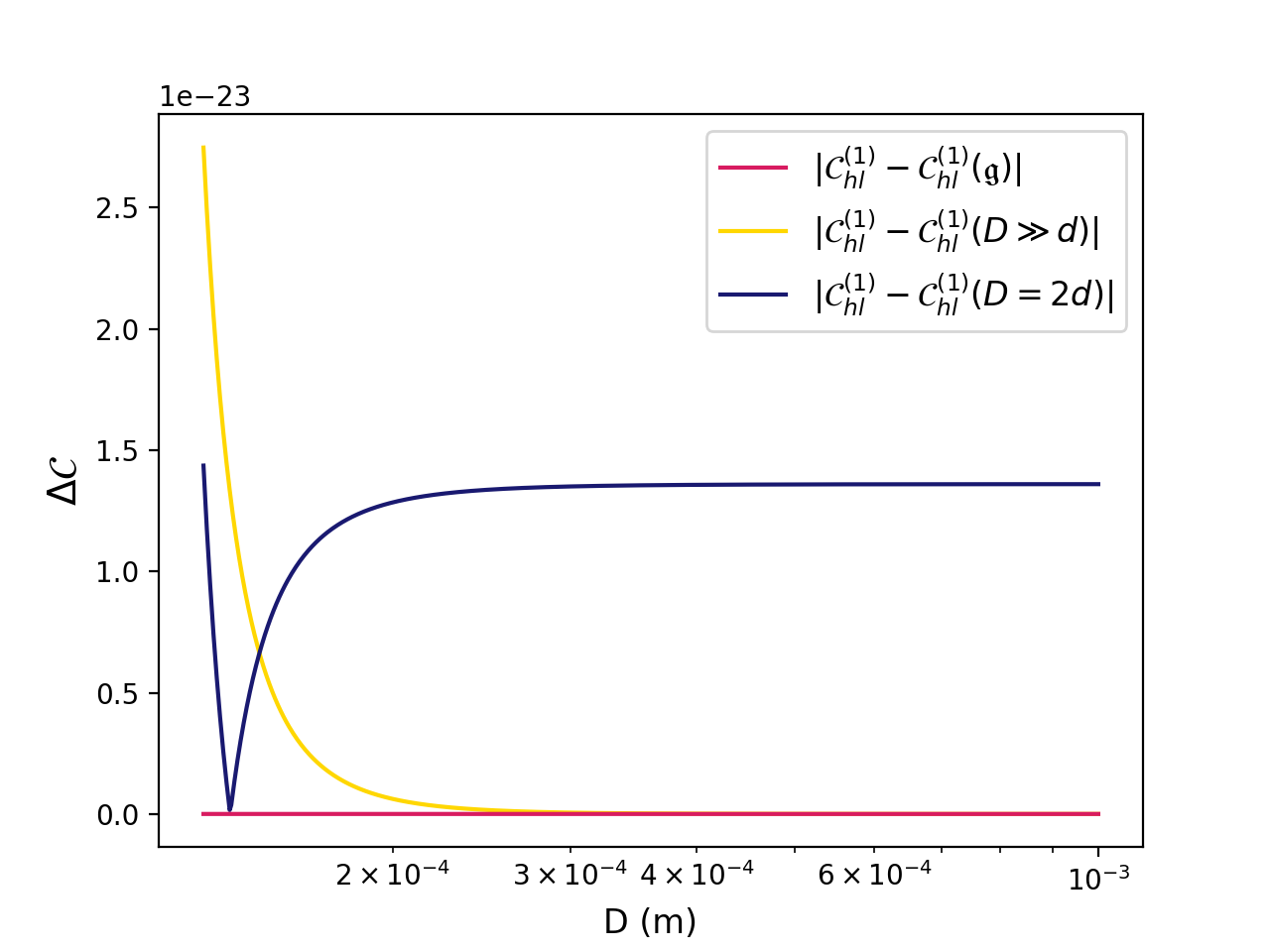
These three limits work in different domains of $d/D$. In Fig. 2 we compare the different approximations as a function of $D$. The range of $D$ shown is from $d$ (which is taken to be of the order $10^{-4}$ m, following (Bose:2022uxe)) to $10^{-3}$ m, the lines continue to be a constant for a larger $D$. As one would expect, the concurrence $\mathcal{C}_{D=2d}$ is the worst approximation (except when $D=2d$). The concurrence $\mathcal{C}_{\mathfrak{g}}$ performs the best across the whole range. Although the concurrence $\mathcal{C}_{D\gg d}$ starts performing well around $D\sim 10^{-3}$ m as well. We have explored and analysed these limits in order to be able to perform an analytical analysis in Sec. VI.

The concurrence quantifies the entanglement due to the coupling between the light and heavy system. Since entanglement and decoherence are two sides of the same coin, the concurrence between the subsystems provides a handle on the decoherence behaviour of the test masses due to the presence of the apparatus. If there is no interaction between the heavy and light subsystems ($\mathfrak{g}_{\pm}=0$), then there is no gravitational decoherence from the experimental apparatuses. However, in any experiment the gravitational decoherence due to the experimental apparatus is unavoidable. Minimizing the mass $M$, and maximizing the trap frequency $\omega$, as well as the distance $D$, minimizes the decoherence from the apparatuses.

At first order the coupling between the heavy and light systems is only between the position operators (it is a quadratic coupling in the Hamiltonian, i.e, linear equations of motion). We now look at the post-Newtonian corrections which contains also momentum operators, focusing on cubic couplings in the Hamiltonian (quadratic couplings in the equations of motion) Inserting the position operators in Eqs. (1) and (2) into the Hamiltonian given in Eq. (62), we obtain the cubic couplings in Eq. (63), where we consider only the next order coupling between the light and heavy matter systems ¹⁵¹⁵ 15 The heavy-heavy and light-light couplings can be seen as self-interactions for the light-heavy bipartition used to calculate $\mathcal{C}_{\text{hl}}$. . This expression contains the couplings between three operators: two light momentum/position operators and one heavy position operator, or two heavy position operators and one light position operator. The relevant non-zero coefficients for the final wavefunction defined in Eq. (19) can be found the same way as before, by filling in the mode operators of Eq.(6) into the interaction Hamiltonian in Eq. (62). We find the following nonzero terms:

	$\displaystyle C_{0102}=C_{1020}$	$\displaystyle=\frac{\mathfrak{g}^{-}_{1}}{2\omega_{h}+\omega_{l}}\,,$		(48)
	$\displaystyle C_{0120}=C_{1002}$	$\displaystyle=-\frac{\mathfrak{g}^{+}_{1}}{2\omega_{h}+\omega_{l}}\,,$		(49)
	$\displaystyle C_{0201}=C_{2010}$	$\displaystyle=\frac{\mathfrak{g}^{-}_{3}-\mathfrak{g}^{-}_{2}}{\omega_{h}+2\omega_{l}}\,,$		(50)
	$\displaystyle C_{0210}=C_{2001}$	$\displaystyle=\frac{\mathfrak{g}^{+}_{2}-\mathfrak{g}^{+}_{3}}{\omega_{h}+2\omega_{l}}\,,$		(51)

with the six different couplings defined by:

	$\displaystyle\mathfrak{g}^{\pm}_{1}$	$\displaystyle=\frac{12\sqrt{2}G}{\omega_{h}(D\pm d)^{4}}\sqrt{\frac{m\hbar}{\omega_{l}}}\,,$		(52)
	$\displaystyle\mathfrak{g}^{\pm}_{2}$	$\displaystyle=\frac{12\sqrt{2}G}{\omega_{l}(D\pm d)^{4}}\sqrt{\frac{M\hbar}{\omega_{h}}}\,,$		(53)
	$\displaystyle\mathfrak{g}^{\pm}_{3}$	$\displaystyle=\frac{3G\omega_{l}}{\sqrt{2}c^{2}(D\pm d)^{2}}\sqrt{\frac{M\hbar}{\omega_{h}}}\,.$		(54)

The "$-$"-labelled couplings arise due to interactions between neighbouring heavy and light oscillators, while the "$+$"-labelled couplings arise due to maximally separated heavy and light oscillators. Moreover, we underline the fact that the $\mathfrak{g}_{3}$ couplings represent the interaction of two momentum operators with a position operator, while the $\mathfrak{g}_{1}$ and $\mathfrak{g}_{2}$ couplings are attributable to the product of three position operators.

References

- (1) Will, C. The confrontation between general relativity and experiment. Living Reviews In Relativity. 17, 1-117 (2014)
- (2) B. P. Abbott et al. [LIGO Scientific and Virgo], “Observation of Gravitational Waves from a Binary Black Hole Merger,” Phys. Rev. Lett. 116 (2016) no.6, 061102 doi:10.1103/PhysRevLett.116.061102 [arXiv:1602.03837 [gr-qc]].
- (3) S. W. Hawking and G. F. R. Ellis, “The Large Scale Structure of Space-Time,” Cambridge University Press, 2011, ISBN 978-0-521-20016-5, 978-0-521-09906-6, 978-0-511-82630-6, 978-0-521-09906-6 doi:10.1017/CBO9780511524646
- (4) N. E. Bjerrum-Bohr, “Quantum gravity, effective fields and string theory,” [arXiv:hep-th/0410097 [hep- th]]. Thiemann:2006cf
- (5) T. Thiemann, Lect. Notes Phys. 721 (2007), 185-263 doi:10.1007/978-3-540-71117-9_10 [arXiv:hep-th/0608210 [hep-th]].
- (6) Amelino-Camelia, G. Quantum-spacetime phenomenology. Living Reviews In Relativity. 16, 1-137 (2013)
- (7) F. Dyson, “Is a graviton detectable?,” Int. J. Mod. Phys. A 28 (2013), 1330041 doi:10.1142/S0217751X1330041X
- (8) Dewitt, Cécile Morette and Dean Rickles. “The role of gravitation in physics : report from the 1957 Chapel Hill Conference.” (2011).
- (9) S. Bose, A. Mazumdar, G. W. Morley, H. Ulbricht, M. Toroš, M. Paternostro, A. Geraci, P. Barker, M. S. Kim and G. Milburn, “Spin Entanglement Witness for Quantum Gravity,” Phys. Rev. Lett. 119 (2017) no.24, 240401 doi:10.1103/PhysRevLett.119.240401 [arXiv:1707.06050 [quant-ph]].
- (10) C. Marletto and V. Vedral, “Gravitationally-induced entanglement between two massive particles is sufficient evidence of quantum effects in gravity,” Phys. Rev. Lett. 119 (2017) no.24, 240402 doi:10.1103/PhysRevLett.119.240402 [arXiv:1707.06036 [quant-ph]].
- (11) J. F. Donoghue, “General relativity as an effective field theory: The leading quantum corrections,” Phys. Rev. D 50 (1994), 3874-3888 doi:10.1103/PhysRevD.50.3874 [arXiv:gr-qc/9405057 [gr-qc]].
- (12) S. Bose, A. Mazumdar, M. Schut and M. Toroš, “Mechanism for the quantum natured gravitons to entangle masses,” Phys. Rev. D 105 (2022) no.10, 106028 doi:10.1103/PhysRevD.105.106028 [arXiv:2201.03583 [gr-qc]].
- (13) C. H. Bennett, D. P. DiVincenzo, J. A. Smolin and W. K. Wootters, “Mixed state entanglement and quantum error correction,” Phys. Rev. A 54 (1996), 3824-3851 doi:10.1103/PhysRevA.54.3824 [arXiv:quant-ph/9604024 [quant-ph]].
- (14) R. J. Marshman, A. Mazumdar and S. Bose, “Locality and entanglement in table-top testing of the quantum nature of linearized gravity,” Phys. Rev. A 101 (2020) no.5, 052110 doi:10.1103/PhysRevA.101.052110 [arXiv:1907.01568 [quant-ph]].
- (15) Christodoulou, Marios, Andrea Di Biagio, Markus Aspelmeyer, Časlav Brukner, Carlo Rovelli, and Richard Howl. "Locally mediated entanglement through gravity from first principles." arXiv preprint arXiv:2202.03368 (2022).
- (16) D. L. Danielson, G. Satishchandran and R. M. Wald, “Gravitationally mediated entanglement: Newtonian field versus gravitons,” Phys. Rev. D 105 (2022) no.8, 086001 doi:10.1103/PhysRevD.105.08600
- (17) D. Biswas, S. Bose, A. Mazumdar and M. Toroš, “Gravitational Optomechanics: Photon-Matter Entanglement via Graviton Exchange,” [arXiv:2209.09273 [gr-qc]].
- (18) R. J. Marshman, A. Mazumdar, R. Folman and S. Bose, “Constructing nano-object quantum superpositions with a Stern-Gerlach interferometer,” Phys. Rev. Res. 4 (2022) no.2, 023087 doi:10.1103/PhysRevResearch.4.023087 [arXiv:2105.01094 [quant-ph]].
- (19) Y. Margalit, O. Dobkowski, Z. Zhou, O. Amit, Y. Japha, S. Moukouri, D. Rohrlich, A. Mazumdar, S. Bose and C. Henkel, et al. “Realization of a complete Stern-Gerlach interferometer: Towards a test of quantum gravity,” doi:10.1126/sciadv.abg2879 [arXiv:2011.10928 [quant-ph]].
- (20) R. Zhou, R. J. Marshman, S. Bose and A. Mazumdar, “Catapulting towards massive and large spatial quantum superposition,” [arXiv:2206.04088 [quant-ph]].
- (21) T. W. van de Kamp, R. J. Marshman, S. Bose and A. Mazumdar, “Quantum Gravity Witness via Entanglement of Masses: Casimir Screening,” Phys. Rev. A 102 (2020) no.6, 062807 doi:10.1103/PhysRevA.102.062807 [arXiv:2006.06931 [quant-ph]].
- (22) H. Chevalier, A. J. Paige and M. S. Kim, “Witnessing the nonclassical nature of gravity in the presence of unknown interactions,” Phys. Rev. A 102 (2020) no.2, 022428 doi:10.1103/PhysRevA.102.022428 [arXiv:2005.13922 [quant-ph]].
- (23) P. F. Barker, S. Bose, R. J. Marshman and A. Mazumdar, “Entanglement based tomography to probe new macroscopic forces,” [arXiv:2203.00038 [hep-ph]].
- (24) M. Toroš, T. W. Van De Kamp, R. J. Marshman, M. S. Kim, A. Mazumdar and S. Bose, “Relative acceleration noise mitigation for nanocrystal matter-wave interferometry: Applications to entangling masses via quantum gravity,” Phys. Rev. Res. 3 (2021) no.2, 023178 doi:10.1103/PhysRevResearch.3.023178 [arXiv:2007.15029 [gr-qc]].
- (25) M. Schut, J. Tilly, R. J. Marshman, S. Bose and A. Mazumdar, “Improving resilience of quantum-gravity-induced entanglement of masses to decoherence using three superpositions,” Phys. Rev. A 105 (2022) no.3, 032411 doi:10.1103/PhysRevA.105.032411 [arXiv:2110.14695 [quant-ph]].
- (26) J. Tilly, R. J. Marshman, A. Mazumdar and S. Bose, “Qudits for witnessing quantum-gravity-induced entanglement of masses under decoherence,” Phys. Rev. A 104 (2021) no.5, 052416 doi:10.1103/PhysRevA.104.052416 [arXiv:2101.08086 [quant-ph]].
- (27) J. S. Pedernales, G. W. Morley, and M. B. Plenio, Physical Review Letters 125, 023602 (2020).
- (28) M. Toroš, A. Mazumdar and S. Bose, “Loss of coherence of matter-wave interferometer from fluctuating graviton bath,” [arXiv:2008.08609 [gr-qc]].
- (29) S. Rijavec, M. Carlesso, A. Bassi, V. Vedral and C. Marletto, “Decoherence effects in non-classicality tests of gravity,” New J. Phys. 23 (2021) no.4, 043040 doi:10.1088/1367-2630/abf3eb [arXiv:2012.06230 [quant-ph]].
- (30) G. Torrieri, [arXiv:2210.08586 [gr-qc]].
- (31) R. Zhou, R. J. Marshman, S. Bose and A. Mazumdar, “Mass Independent Scheme for Large Spatial Quantum Superpositions,” [arXiv:2210.05689 [quant-ph]].
- (32) M. Schlosshauer, “Decoherence, the Measurement Problem, and Interpretations of Quantum Mechanics,” Rev. Mod. Phys. 76 (2004), 1267-1305 doi:10.1103/RevModPhys.76.1267 [arXiv:quant-ph/0312059 [quant-ph]].
- (33) S.N Gupta, Quantization of Einstein’s Gravitational Field: Linear Approximation Proc. Phys. Soc. A 65 161, 1952.
- (34) W. K. Wootters, “Entanglement of formation of an arbitrary state of two qubits,” Phys. Rev. Lett. 80 (1998), 2245-2248 doi:10.1103/PhysRevLett.80.2245 [arXiv:quant-ph/9709029 [quant-ph]].
- (35) G. Grignani, T. Harmark, M. Orselli and A. Placidi, “Fixing the non-relativistic expansion of the 1PM potential,” JHEP 12 (2020), 142 doi:10.1007/JHEP12(2020)142 [arXiv:2006.13234 [hep-th]].
- (36) Y. Iwasaki, “Quantum theory of gravitation vs. classical theory. - fourth-order potential,” Prog. Theor. Phys. 46 (1971), 1587-1609 doi:10.1143/PTP.46.1587
- (37) A. Cristofoli, N. E. J. Bjerrum-Bohr, P. H. Damgaard and P. Vanhove, “Post-Minkowskian Hamiltonians in general relativity,” Phys. Rev. D 100 (2019) no.8, 084040 doi:10.1103/PhysRevD.100.084040 [arXiv:1906.01579 [hep-th]].
- (38) B. R. Slezak, et al, “Cooling the motion of a silica microsphere in a magneto-gravitational trap in ultra-high vacuum,” New Journal of Physics 20.6 (2018): 063028.
- (39) V. Balasubramanian, M. B. McDermott and M. Van Raamsdonk, “Momentum-space entanglement and renormalization in quantum field theory,” Phys. Rev. D 86 (2012), 045014 doi:10.1103/PhysRevD.86.045014 [arXiv:1108.3568 [hep-th]].
- (40) M. Schlosshauer, “The quantum-to-classical transition and decoherence,” [arXiv:1404.2635 [quant-ph]].
- (41) A. Pathak, “Elements of quantum computation and quantum communication,” Boca Raton: CRC Press, 2013, ISBN 978-1-4665-1792-9
- (42) S. Hill and W. K. Wootters, “Entanglement of a pair of quantum bits,” Phys. Rev. Lett. 78 (1997), 5022-5025 doi:10.1103/PhysRevLett.78.5022 [arXiv:quant-ph/9703041 [quant-ph]].
Appendix A Equations
Interaction Hamiltonian between the heavy and light system, after a non-relativistic expansion upto and at first order in :