Multiple gas phases in supernova remnant IC 443: mapping shocked with VLT/KMOS2022 Affiliation: School of Astronomy and Space Science, Nanjing University, Nanjing 210093, People’s Republic of China Multiple gas phases in supernova remnant IC 443: mapping shocked with VLT/KMOS–4 Affiliation: School of Astronomy and Space Science, Nanjing University, Nanjing 210093, People’s Republic of China
Abstract
Supernovae and their remnants provide energetic feedback to the ambient interstellar medium (ISM), which is often distributed in multiple gas phases. Among them, warm molecular hydrogen () often dominates the cooling of the shocked molecular ISM, which has been observed with the emission lines at near-infrared wavelengths. Such studies, however, were either limited in narrow filter imaging or sparsely sampled mid-infrared spectroscopic observations with relatively poor angular resolutions. Here we present near-infrared (- and -band) spectroscopic mosaic observations towards the A, B, C, and G regions of the supernova remnant (SNR) IC 443, with the K-band Multi-Object Spectrograph (KMOS) onboard the Very Large Telescope (VLT). We detected 20 ro-vibrational transitions of , one H line (Br), and two [Fe ii] lines, which dominate broadband images at both - and -band. The spatial distribution of lines at all regions are clumpy on scales from pc down to pc. The fitted excitation temperature of is between 1500 K and 2500 K, indicating warm shocked gas in these regions. The multi-gas-phase comparison shows stratified shock structures in all regions, which explains the co-existence of multiple types of shocks in the same regions. Last, we verify the candidates of young stellar objects previously identified in these regions with our spectroscopic data, and find none of them are associated with young stars. This sets challenges to the previously proposed scenario of triggered star formation by SNR shocks in IC 443.
Keywords:
: ISM: individual objects: IC 443 – ISM: supernova remnants – ISM: molecules – shock wave1 Introduction
Supernova feedback to the interstellar medium (ISM) plays a key role during the evolution of stars and galaxies (Hopkins et al. 2014; Koo et al. 2020). Massive stars are born from molecular clouds and interact with their ambient natal ISM throughout their lives (Lada & Lada 2003; Krumholz et al. 2019). Core Collapse Supernova remnants (SNRs), as the end of massive stars, play a significant role in these processes, generating large amounts of shock, radiation, and heavy metals. These processes would compress, heat up, dissociate, and ionize their surrounding molecular clouds (MCs), and distribute heavy elements throughout the galaxies. SNRs are also important sources of accelerating cosmic rays which can heat the dense cores of the MCs. Interaction between SNRs and giant molecular clouds (GMCs) may enhance (Ikeuchi et al. 1984; Leonidaki et al. 2013) or suppress (Dekel et al. 2019) sequential star-formation, and then regulate the evolution of galaxies.
Supernova shock provides energetic feedback to the ISM (Draine & McKee 1993). These shocks carry a significant amount of mechanical energy which gradually dissipate in turbulence as the shocks propagate through and interact with the ambient ISM. They can heat, compress and accelerate the gas in GMCs and may turn the gas into different phases (, H i, and H+) with a wide range of shock parameters: of several in velocity, in volume density, and K in temperature (McKee & Hollenbach 1980). These processes lead to a wide variety of structures and observables.
IC 443, also named as the Jellyfish Nebula from its optical morphology, is a mixed-morphology SNR located in the galactic anti-centre (see Rho & Petre 1998; Jones et al. 1998, for references). IC 443 has a diameter of at the optical and radio bands and is thought to contact with the Gem OB1 association at a distance of 1.5-2.0 kpc (Carpenter et al. 1995). We adopt 1.6 kpc from the measurement of Gaia Data Release 2 (DR2) parallax and dust extinction (Zucker et al. 2020). IC 443 originated from a core-collapse supernova explosion, with a large uncertainty in its age (– yr) (Chevalier 1999; Olbert et al. 2001; Troja et al. 2008),
With clear evidence of impacts with nearby surrounding MCs, IC 443 provides a unique test field of shock conditions in the Milky Way. The shock processes are not only accelerating and stratifying molecular gas, but also powering atomic and ionized gas phases with strong and extremely broad emission lines. These shock features have been detected in CO, , H i, etc. (Denoyer 1979; Dickman et al. 1992; Snell et al. 2005; Lee et al. 2008; Zhang et al. 2010, e.g.), which show broadening features in almost all gas clumps, especially the B, C, and G regions (Huang et al. 1986, following the nomenclature of). observations (Snell et al. 2005) further show that a variety of shock types and velocity components are required.
As the most abundant molecule in the ISM, molecular hydrogen is therefore the major molecule in the shock-MC interacting regions. As a homo nuclear molecule, has no permanent dipole electric moment. Because of this, can only emit with its electric quadrupole transitions at infrared wavelengths, that are more easily reachable with space-based instruments. Using the long-slit mid-IR echelle spectrometer onboard NASA Infrared Telescope Facility (IRTF), Richter et al. 1995a detected 0-0 S(2) rotational transition at 12.28 m towards the C clump of IC 443, and confirmed the presence of a partially dissociating J-shock. Based on a time-dependent shock model, Cesarsky et al. 1999 measured intensities of pure rotational lines with the Infrared Space Observatory (ISO) and found a fast shock with short timescales of 1000–2000 years; Shinn et al. 2011 proposed a scheme of the co-existence of both C- and J-shocks that “the C-type shocks propagate into ‘clumps’, while J-type propagate into ‘clouds’ (inter-clump medium)”.
Besides the pure rotational transitions, the rotational-vibrational (hereafter ro-vibrational) transitions of molecules are also often seen in shocked regions. The first energy level for ro-vibrational transitions is 1-0 S(0) (-, -) with an upper level energy of K, allowing it to trace warm molecular gas at temperature K.
Though the warm and hot can only make up a small mass fraction of all the shocked , it plays an important role as the major coolant in molecular shocks (Flower & Pineau Des Forêts 2010; Lehmann et al. 2020). The cooling processes become much more efficient at a higher temperature because the cooling efficiency of at K is about three orders of magnitude larger than that at K (Le Bourlot et al. 1999).
The shocked molecular gas of IC 443 mainly distributes in an incomplete ring shape, with a bright -shaped ridge in the south. It consists of several bright clumps, namely A, B, C, D, etc., which seem to be connected with more extended and fainter emission. Lee et al. 2012 interpreted these small gas clumps as dense cores from their parental MCs, where the progenitor star of IC 443 was formed. From narrow-band mapping observations of 1-0 S(1), Burton et al. 1988 found that the emission comes from a sinuous ridge where the molecular hydrogen is directly shocked by the supernova shock wave. The spatial distribution of shocked is remarkably similar to the high-velocity CO, , and HCN molecules.
Reach et al. 2019 made high-resolution (R=67000) observations of pure rotational lines and found that, to best fit the observed S(5) line profile, a multi-component shocks (CJ-type shocks combined with J-type shocks at gas densities of –) are needed.
Burton et al. 1988, Rho et al. 2001, and Kokusho et al. 2020 have mapped the 1-0 S(1) and 2-1 S(1) transitions of IC 443 with broadband or narrowband filters. Although these imaging observations detected a significant amount of ro-vibrational lines emission, they could not distinguish the contribution from each line and could not derive the population of vibrational levels. On the other hand, Richter et al. 1995b and Shinn et al. 2011 observed several ro-vibrational lines in IC 443 with a long-slit spectrograph. However, the sizes of the slits only gave limited fields of view (FoVs) to resolve detailed spatial structures. Integral field spectroscopic observations, which offer both moderate spectral resolution and wide FoV into account, are required to simultaneously map multiple transitions.
Furthermore, it has been debated whether SNRs and their progenitors could trigger star formation in their surrounding clouds on fairly short timescales. Xu et al. 2011 proposed star formation would be triggered by the expansion of IC 443, by identifying candidates of protostellar objects and young stellar objects (YSOs), based on Infrared Astronomical Satellite IRAS Point Source Catalog and the Two Micron All Sky Survey (Skrutskie et al. 2006, 2MASS,). Similarly, Su et al. 2014 selected YSO candidates based on 2MASS and Wide-field Infrared Survey Explorer (Wright et al. 2010, WISE,) databases using a colour-colour diagram. More recently, Dell’Ova et al. 2020 combined Gaia, WISE, and 2MASS databases and selected protostar candidates with colour-colour filtering method in the IC 443 G region, where they propose to have a higher concentration of protostar candidates in the shocked clump. However, all these photometric selected YSO candidates still need to be verified with spectroscopic observations at near-IR wavelengths. The K-band Multi-Object Spectrograph (KMOS) onboard the Very Large Telescope (VLT) offers an opportunity to testify if the candidates are real.
In this paper, we report near-infrared mapping results of ro-vibrational transitions of , Br line, and [Fe ii] lines over regions A, B, C, and G in IC 443, using KMOS onboard VLT. In Section 2, we describe information on the KMOS observations and data. We then describe the results and analysis of the lines observed in these four regions in Section 3. In Section 4, we compare our data with mid-infrared pure rotational lines and with the distributions of neutral gas and cold traced by H i and CO. We also discuss the contribution of the ro-vibrational lines at band and falsify the YSO candidates in the G region. Finally, in Section 5, we make a brief conclusion and prospect our future design about our multi-wavelength campaign which is aiming to build a panchromatic perspective of IC 443 from the observational aspect by combining our CO, H i, and H data.

2 Observations and data reduction
2.1 Choice of regions
We select four molecular clumps of IC 443, regions A, B, C, and G (see Figure 1), as our targets of KMOS observations. Among them, IC 443 B, C, and G have been detected with the most prominent broadened CO features of angular sizes (Wang & Scoville 1992; van Dishoeck et al. 1993; Zhang et al. 2010, e.g.). Although IC 443 A does not show a broad CO emission, it has a prominent high-velocity emission (Dickman et al. 1992) and H emission (see Section 4.3.1).
From the currently known geometry and kinematic structures (van Dishoeck et al. 1993, e.g.), shocks in region A, B, and C are propagating mostly along the line of sight and are reaching gas clumps in succession. Shocks in the G region, on the other hand, propagate perpendicular to the line of sight.
2.2 KMOS data
2.2.1 Observations
Our observations (Program ID: 0104.C-0924, PI: Zhi-Yu Zhang) were performed with the near-infrared K-band Multi-Object Spectrograph (Sharples et al. 2013, KMOS,) onboard the Very Large Telescope (VLT) at Cerro Paranal in Chile, during December 2019 and January 2020.
KMOS has 24 configurable arms, of each an integral field unit (IFU) is employed. Each IFU has 1414 pixels with a spatial sampling 0.2, thus a spatial coverage of of 2.8. We adopted the Mosaic Mode to carry out the mapping observations, which arrange the 24 arms in a 64 grid of fixed dimensions. For each scan, the telescope move across 16 successive telescope pointings, which allows a complete mosaic of data covering a region of .
We use the HK grating to cover both and bands simultaneously (from 1.46 m to 2.41 m ). It offers a spectral resolution of , which correspond to a velocity resolution of km s-1 at 2 m .
The observations were performed with eight observing blocks (OBs). Each mosaic scan consists of 16 successive telescope pointings and exposures. For each of the 16 pointings, we spent 150 s on source and 150 s for sky exposure. Such an observational configuration maximises the mapping area but all pixels have only a single exposure, except for the pixels in the overlap regions of two IFUs. During our observations, unfortunately, one of the 24 arms was not functional 11 1 http://www.eso.org/sci/facilities/paranal/instruments/kmos/news.html, leaving a rectangular empty area in the datacube at each region (white squares in Figure 3).
All nights have conditions of clear skies (or better) and good sky transparency. The precipitable water vapour (PWV) was 3.0 mm on average and the seeing ranges from to for different mosaic exposures, with a mean of . Only one mosaic exposure in region A was taken with seeing larger than .
2.2.2 Data Reduction
All mosaic data were initially reduced using the ESO KMOS pipeline
(Davies
et al. 2013, ver. kmos-3.0.1 ) integrated into the
interactive pipeline operating environment ESO Reflex: ESO Recipe Flexible
Execution Workbench (Freudling et al. 2013, esoreflex-2.11.0;).
ESO Reflex can automatically perform most of the main reduction steps including
dark, flat, wavelength calibration, luminosity correction, telluric and
atmospheric correction, flux calibration, and cube reconstruction and
combination, etc. The calibration data we adopted was delivered with the
pipeline and the ESO CalSelector
service22
2
https://archive.eso.org/cms/application_support/calselectorInfo.html.
We use a spatial sampling rate of per pixel and a spectral sampling
rate of nm per channel to reconstruct the 3-D data cubes, satisfying a
Nyquist sampling. The consequent velocity sampling rate is 84 km s-1
for 1.6440 m [Fe ii] line and 70 km s-1 for 2.1218 m
1-0 S(1) line.
Because each pixel was observed only once, the error was not properly propagated in the pipeline. To obtain a channel-based noise, the uncertainties of line intensities are estimated by the standard deviation of a moving-box that contains 20 line-free channels at both sides of each line, and this is regarded as the uncertainties for all the line channels. Our estimated is on the order of erg s-1 cm-2 Å-1 per pixel per channel. After examining with stars observed in our data with the 2MASS catalog, we adopt an uncertainty of 20% in the absolute flux calibration, which is consistent with the 5-20% uncertainty suggested by the KMOS user manual.
During combining all cubes produced from subscans, the mosaic tessellation sometimes is not always perfect because of the errors of pointing, and sometimes the pipeline makes the seams of the mosaic sub-cubes with unnaturally bright structures, especially in regions A and G (see Figure 3).
Therefore, we masked the apparent abruption and misplacement visually found in the final mosaic cube. The OH line subtraction is not optimal in some cases, especially for region G. We further subtract the median value of nearby line-free pixels to remove the remaining radiance features.
The vapour leads to an enhanced atmospheric absorption of almost zero transmission nearby 1.87m, depending on the PWV (See Figure 2). In the following analysis, we simply abandon all lines that are severely affected by absorption. Although some lines in this wavelength range seem to be well detected, their fluxes have too high uncertainties to be trusted.
2.3 Ancillary Data
In this work, we compare the KMOS data with H i 21-cm data from the Karl G. Jansky Very Large Array (JVLA), the old VLA, and the Arecibo telescopes, CO =3-2 from the James Clerk Maxwell Telescope (JCMT), H data from the SITELLE onboard the Canada-France-Hawaii Telescope (CFHT), and r band data from the Zwicky Transient Facility (ZTF).
The VLA/JVLA 21-cm Hi data consists of multiple observations taken with the B, C, and D array configurations. Among them, the JVLA B- and C-array observations are performed in 2016 (Project ID: 16A-266, PI: Ping Zhou). The D-array observation is performed in 2001 (Lee et al. 2008, Project ID: AK0537,). The Arecibo 21-cm Hi data is acquired from the GALFA-H i survey DR 1 (Peek et al. 2011). We combined all VLA/JVLA and Arecibo data with the Total Power Map To Visibilities packages (Koda et al. 2019, TP2VIS,), and image it with Common Astronomy Software Applications version 6.1.2.7 (CASA) (McMullin et al. 2007). Details about the observations and data reduction will be reported in a separate paper (Lin et al. in prep.).
The CO =3-2 data was observed in November 2015 with submillimetre spectral imaging system HARP/ACSIS Buckle et al. 2009 onboard JCMT (Proposal ID: M15BI126) and we download the reduced data from the JCMT science archive.
The CFHT/SITELLE data are performed in 2021 (Project ID: 21BS020, PI: Yunwei Deng). SITELLE is an imaging Fourier transform spectrometer which offers large FoV and high-spectral resolution simultaneously (Drissen et al. 2019). IC 443 A and B were observed in the SN3 band with a spectral resolution of . We extract the moment-0 maps of H emission to multi-band comparison. For the C and G regions of IC 443, we download the ZTF r band data from the IRSA ZTF archive (Masci et al. 2019) as a substitution to trace H emission.
In Section 4.5, we use catalogs from Gaia eDR3 (Gaia Collaboration et al. 2021) and LAMOST DR7 (Luo et al. 2015) to help analyze the YSO candidates.
3 Results
3.1 Near Infrared emission lines in shocked regions
In Figure 2, we present spectra averaged spatially in all four regions. All regions show strong line emission with a total of 23 detected lines and almost no continuum emission. The background grey lines are the atmospheric transmission at Paranal with PWV=3.5 obtained from ESO SkyCalc33 3 https://www.eso.org/observing/etc/bin/gen/form?INS.MODE=swspectr+INS.NAME=SKYCALC. The spectrum of region G seems to exhibit more line features at the -band, which are dominated by the residuals of OH lines from the atmospheric features. In Figure 17, we plot the atmospheric radiance with PWV=3.5 obtained from ESO SkyCalc (refer to Rousselot et al. 2000, for the OH line catalog). Table 1 lists the intensity of the detected lines in these regions. Although the lines between 1.80 m and 1.96 m seem to be well detected (Figure 2), especially on the bright structures, their fluxes are highly biased by the imperfect atmospheric corrections. Though these lines are listed in Table 1, we do not use them in the discussion. The 1-0 S(10) and S(11) lines are too weak in the spatially averaged spectra. However, they are detected in the bright knots in regions A, C, and G (e.g. knots mentioned in Section 3.1.1 and listed in Table 4), so we still list them in Table 1 as detected lines.
Most of the near-infrared emission in these molecular clumps comes from the ro-vibrational transitions of shock disturbed warm molecular hydrogen. By cross-checking our observed emission lines with the list of lines compiled by Roueff et al. 2019, we identified a total of 20 ro-vibrational lines with a signal-to-noise ratio (S/N) higher than five, including 1-0 S(0) through S(11), 2-1 S(0) through S(5), and transitions of 3-2 S(3) and S(5), in these four regions. Among these lines, the 1-0 S(4), 1-0 S(5), and 2-1 S(4), 2-1 S(5) transitions seem to be attenuated by atmospheric absorptions. Although the 1-0 S(3) line lies in a narrow atmospheric window, which means that its flux might be able to be corrected, we find still large uncertainties in the correction, especially in region A (Section 3.1.1). Therefore, we ignore these five lines in the following analysis, because of the large uncertainty in their fluxes.
Near-infrared recombination lines of hydrogen – Pa and Br (and a few higher transitions in the Br series, up to Br10) – are covered by the HK grating. Unfortunately, all these lines are attenuated by the atmospheric absorption, except for Br at 2.1661 m, which was only detected in region A (see details in Section 3.1.2).
Similarly, strong [Fe ii] 1.6440 m line and [Fe ii] 1.8099 m line are detected in region A (see Section 3.1.3). Nonetheless, [Fe ii] 1.8099 m is attenuated by the atmosphere features. In regions B, C, and G, the [Fe ii] 1.6440 m lines are detected, while the [Fe ii] 1.8099 m line is only marginal detected in region C and shows non-detections in region B and G.
| Transition | (m) | (K) | Line Intensity ( erg s-1 cm-2 sec-2) | |||
| A | B | C | G | |||
| 1-0 S(11) | 1.6504 | 18979.1 | … | … | … | … |
| 1-0 S(10) | 1.6665 | 17310.8 | … | … | … | … |
| 1-0 S(9) | 1.6877 | 15721.5 | … | |||
| 1-0 S(8) | 1.7147 | 14220.5 | … | |||
| 1-0 S(7) | 1.7480 | 12817.3 | ||||
| 1-0 S(6) | 1.7880 | 11521.1 | ||||
| 1-0 S(5)* | 1.8358 | 10341.2 | … | |||
| 1-0 S(4)* | 1.8919 | 9286.4 | … | |||
| 1-0 S(3)* | 1.9576 | 8364.9 | ||||
| 1-0 S(2) | 2.0338 | 7584.3 | ||||
| 1-0 S(1) | 2.1218 | 6951.3 | ||||
| 1-0 S(0) | 2.2233 | 6471.4 | ||||
| 2-1 S(5)* | 1.9449 | 15762.7 | … | … | ||
| 2-1 S(4)* | 2.0041 | 14763.5 | … | … | ||
| 2-1 S(3) | 2.0735 | 13890.2 | ||||
| 2-1 S(2) | 2.1542 | 13150.3 | … | |||
| 2-1 S(1) | 2.2477 | 12550.0 | ||||
| 2-1 S(0) | 2.3556 | 12094.9 | … | |||
| 3-2 S(5) | 2.0656 | 20855.7 | … | … | ||
| 3-2 S(3) | 2.2014 | 19085.8 | ||||
| [Fe ii] | 1.6440 | 11446.0 | … | |||
| [Fe ii]* | 1.8099 | 11446.0 | … | … | … | |
| Br | 2.1661 | 154582.8 | ||||
| Though not be listed here, these lines are detected (e.g. Table 4) and marked in Figure 2. | ||||||
| These lines are attenuated by the atmospheric absorption. Their intensities are likely underestimated. | ||||||
3.1.1 Rotational–vibrational lines
In total, twenty lines were detected in IC 443 A, B, C, and G, ranging from 1.6504 m to 2.3556m. These lines cover a wide range of the upper level energy from 6471.4 K to 20855.7 K.
The four transitions of , from 1-0 S(0) to 1-0 S(3), are the four strongest lines at the band. In regions B, C, and D, the 1-0 S(1) transition, which has an upper level energy K, is the strongest line. In region A, however, the 1-0 S(3) transition ( K) is anomalously stronger than that of 1-0 S(1) (see Figure 2 top panel).
This anomaly leads to the , energy level corresponding to 1-0 S(3) transition is over-populated in region A than levels with either higher or lower energy in the population diagram (see Section 3.2). In fact, the , level appears to be over-populated in all regions with different levels, while the , , , and levels are almost linearly arranged on the population diagrams. The 1-0 S(3) line lays inside the range of the 1.87 m absorption, with high uncertainties in the correction. Therefore, this anomaly is more likely the result of the errors of telluric correction and we exclude this line in the discussions hereafter.
All transitions show similar spatial distributions in the integrated flux maps. In Figure 3, we present spatial distributions of the two most often used near-infrared emission line, 1-0 S(1) and 2-1 S(1) for comparison. These lines are distributed across most regions with filamentary structures on scales less than one arcmin. In all four regions, several small and bright emission clumps (hereafter knots) appear with angular sizes of 1′′–3′′ (0.008-0.024 pc) in diameter.
These knots are all embedded inside extended filamentary and flocculent structures. We label a few representative ones as Ac1, Ac2, Bc1, Bc2, Cc1, Cc2, Gc1, Gc2, Gc3, and Gc4 (see Figure 3). Their positions, and temperature and column density derived by the strongest three transitions (Section 3.2) are listed in Table 2. In Table 4, we list the emission lines detected in these ten small bright clumps.

| R.A. (ICRS) | Dec. (ICRS) | (K) | ||
|---|---|---|---|---|
| Ac1 | 06:16:54.00 | 22:23:02.30 | ||
| Ac2 | 06:16:54.69 | 22:22:55.55 | ||
| Bc1 | 06:17:16.60 | 22:25:26.00 | ||
| Bc2 | 06:17:16.05 | 22:25:18.25 | ||
| Cc1 | 06:17:42.41 | 22:21:22.35 | ||
| Cc2 | 06:17:42.37 | 22:21:15.15 | ||
| Gc1 | 06:16:43.93 | 22:32:52.65 | ||
| Gc2 | 06:16:43.68 | 22:32:29.65 | ||
| Gc3 | 06:16:42.37 | 22:32:10.05 | ||
| Gc4 | 06:16:43.39 | 22:32:06.65 |
3.1.2 The marginal detection of the Br line in region A
Five hydrogen recombination transitions in the Brackett series, Br through Br10, lay in our wavelength coverage. However, the strongest one, 2.1661 m Br, is only detected in region A, which also coincides with the strongest H emission (see Figure 14).
The Br line can hardly be recognized from any single pixel and there are no Br emission structures can be visually found in region A. To increase sensitivity, we stack all data in region A. We estimate the flux uncertainty with 20 nearby line-free channels. The resulted Br intensity is erg s-1 cm-2 arcsec-2, which is one-ninth of the upper limit of Br estimated by Burton et al. 1988 with UKIRT/CVF observations.
Similarly, we also stack Br spectra at regions B, C, and G, respectively, where we only found non-detections. We thus estimate a 3- upper limit of erg s-1 cm-2 arcsec-2 for these three regions. In Figure 4, we present the stacked Br spectra at regions A, B, C, and G. Though H emission is detected in all these regions, the Br emission is absent in regions B, C, and G.
3.1.3 [Fe ii] emission in IC 443 A
[Fe ii] 1.6440 m and 1.8099 m are the only metallic lines detected in our observations. These two lines share the same upper energy level (Koo et al. 2016, , ). In principle, we could derive the foreground dust extinction using their line ratios. However, the 1.8099 m line is heavily attenuated by the atmospheric absorption. Therefore, we focus the 1.6440 m line.
We detect the [Fe ii] 1.6440 m line in all four regions. Among them, the [Fe ii] line is strongest in region A, where diffuse filamentary structures can be roughly recognised in the mom-0 map. As shown in Figure 5, the [Fe ii] 1.644 m line is about one order of magnitude fainter than the strong 1-0 S(1) line.
In Figure 5, we present the spatial distributions of [Fe ii] and in region A, where the two lines seem roughly overlapped with each other, although some regions reveal an anti-correlation between the two lines. This is not consistent with the findings of Kokusho et al. 2020, who found that the spatial distribution of [Fe ii] and in IC 443 are anti-correlated. This is most likely because in region A the shock propagates along the line of sight and the [Fe ii] and emission regions are stratifying as successive layers on the line of sight.
In Figure 6, we present the observed line profiles of Fe ii 1.6440 m line (blue) and 1-0 S(1) 2.1218 m line (red) extracted from a horizontal stripe (Figure 5, white stripe) where both [Fe ii] and emission are strong. With the very limited velocity resolution, it is difficult to study the detailed kinematic difference between [Fe ii] and lines. However, we can still identify that both lines show negative average velocity. The stacked [Fe ii] line covers a high velocity range from 225 km s-1 to 250 km s-1. Since the velocity profile of shocked lines is not expected to be Gaussian, we use 16% and 84% integral flux to describe the line profile. The line width of [Fe ii] 1.6440 m is 201 km s-1, which is 1.86 that of 1-0 S(1) (108 km s-1).
3.2 Population diagrams
The near-infrared lines of molecular hydrogen are optically thin (discussed in Section 4.1), so the column density of at each energy level can be calculated directly from the extinction-corrected intensity of the specific transition,
| (1) |
where is the Einstein A coefficient of the transition from the upper energy level to the lower energy level , is the line intensity of the transition.
Following Shinn et al. 2011 and Neufeld et al. 2007, based on the results of Richter et al. 1995b, we adopt () for the extinction correction in regions B and C, and () in region G. There is no direct measurement of extinction for region A in the literature. Zhang et al. 2010 find no broaden CO emission in this region, implying a low column density and dust extinction. We therefore adopted an of 2.8 (Fesen & Kirshner 1980, ,), which is the average value of six points spreading over the optical filaments similar to those in region A measured with the Balmer decrement. We adopt an optical total-to-selective extinction ratio, , and correct the extinction using the algorithm developed by Cardelli et al. 1989. The wavelength-integrated flux (moment-0) maps can therefore be converted to the column density distribution of at each particular energy level.
In Figure 7, we present population diagrams of in ten knots, from Ac1 to Gc4. Under LTE conditions, all energy levels share the same excitation temperature and the Maxwell-Boltzmann distribution. The natural logarithm of the column density over statistic weight is linearly related to the energy level ,
| (2) |
where is the total column density, is the partition function of (Popovas & Jørgensen 2016). The populations seem to roughly obey the distribution of LTE. However, two branches of populations appear on these diagrams for transitions with upper level energies higher than 10000 K, suggesting that the levels are more populated than the levels (see Section 4.2 for further discussions).
Nonetheless, the population diagrams in Figure 7 also show that even in these shocked knots, the low energy levels are still in good linearity. Particularly, the three strongest lines (from 1-0 S(0) to S(2)), which correspond to the three lowest energy levels (, , , and ) happen to be very linear in most regions.
Here, we use the population diagram method to analyze the emission under the assumptions of optically thin and LTE (Goldsmith & Langer 1999). As Equation 2 shows, by fitting the straight line of versus , we can directly yield a slope as and an intercept as (total ). The temperature inferred here can be regarded as the excitation temperature for the LTE assumption. In practice, we use the chi-square analysis method to estimate the error of the fitting parameters and propagate them to the temperature and total column density of .
Table 2 presents physical parameters estimated inside these knots, where and are the temperature and column density. Most of these knots show a temperature of about 1500–2500 K and a column density of cm-2. Section 3.2.1 will show that these knots have moderate temperatures with relatively high densities inside those shocked molecular clumps.
3.2.1 Spatial distributions of temperature and column density traced by warm
As a first-order approximation, we take the strongest three transitions, from 1-0 S(0) to S(2), to map the temperature and column density distribution with population diagrams. These transitions have the lowest energies among our observed ro-vibrational transitions, and their upper levels are the most populated. We thus fit the populations acquired by these three lines to map the temperature and column density distribution in IC 443 A B, C, and G. The population diagrams in regions B, C, and G show a good linearity.
To further increase the signal-to-noise ratio (S/N) for extended structures, we adopt an adaptive binning scheme outlined as follows: 1). We re-bin the moment-0 map of 1-0 S(2) transition with the Voronoi tessellation binning method developed by Cappellari & Copin 2003. This binning adaptively resamples our data to an S/N of 15 per bin for the 1-0 S(2) transition. The noise map here is obtained locally for each pixel based on its spectrum (). 2). We apply the same Voronoi mesh obtained earlier to the moment-0 map of the other two transitions. 3). To exclude very large bins on the background (whose signal is mainly contributed by a few source pixels), we set a threshold of and masked the bins that do not satisfy this criterion. 4). We derive the temperature and column density of the bins with at least two lines. 5). We keep the bins with fitted temperature and abandon those with uncertainty less than .
The derived column density can be set as a lower limit of the total column density because shocks tend to populate more molecules in the energy states (see Section 4.2).
In Figures 5, 8, 9, and 10, we present the spatial distributions of the excitation temperature and total column density fitted from the rotation diagrams in the A, B, C, and G regions of IC 443. Figure 11 presents the phase diagrams of the excitation temperature and in these four regions, which all show similar ranges of – K and – cm-2, respectively. The small bright knots (from Ac1 to Gc4) are marked with 1′′ diameter light blue cycles in Figures 5–10 and are shown as red crosses in Figure 11.


Both spatial distributions and phase diagrams present inverse correlation between the temperature and column density in all regions, i.e. places with high temperatures show low column density and vice versa. Figure 11 shows that all those ten bright knots have relatively high column density.

The large-scale extended structure, filaments, and bright knots, which present in the emission maps, can also all be seen in the column density maps of regions B, C, and G. In region A, however, these structures are not seen clearly as other regions, possibly due to the relatively weaker emission. In the following, we describe each region in detail.
IC 443 A: Figure 5 shows the spatial distribution of velocity-integrated flux of 1-0 S(1), temperature, and column density in IC 443 A. This region has the lowest column density among all four fields. Most gas in this region mainly distributes along the R.A. direction, with a few branches extending along the Dec. direction. The south-west and north-east parts show the highest and lowest temperature, reaching K and K, respectively. The overall column density distribution presents an anti-correlated with the temperature. Two knots, Ac1 and Ac2, have a temperature of 1800 K and a column density of .
IC 443 B: Figure 8 shows the spatial distributions of velocity-integrated flux of 1-0 S(1), temperature, and column density in IC 443 B. The warm is mainly distributed in a clump with two bright knots, Bc1 and Bc2, in the centre. The peak column densities of these two knots reach cm-2, while they drop sharply to cm-2, two orders of magnitude lower, on the edge of the whole region. The temperature in the north part of IC 443 B is K, while it reaches 2500 K on the south edge with low column densities. In the north-east of region B, there appears an isolated clump with both relatively low temperature and low column density.
IC 443 C: Region C shows the brightest emission among all four regions. As Figure 9 shows, the majority of emission elongates from the northeast to the southwest, with a width 10′′–20′′ (0.15 pc). Overall, the north-west region shows relatively lower temperature, and the high temperature region concentrates in the south, likely tracing a drastic shock heating on the edge of the gas clump. temperature ranges from 1000 to more than 3500 K in temperature and from to cm-2.
Bright knots Cc1 and Cc2 are enclosed in the trunk, showing high column densities and temperature gradients. Cc2 is located close to the hot peak with more than K and a temperature gradient like a cooling front can be found. The emission is abrupt in front of the cooling front, which suggests that the molecular hydrogen has not yet been disturbed and heated by shock waves. Another possible explanation of this abruption is that there is a sharp boundary of the molecular gas, while this did not coincide with the extended CO distribution (see Figure 14). The temperature decreases to K to the northwest and the transverse cooling length can be estimated as pc (). This also gives a lower limit of the length of the post-shock warm zone, which agrees on the order of magnitude with the distance of a shock front with a velocity of would travel in yr (Reach et al. 2019).
In the north region of IC 443 C, the temperature decrease to less than K gradually with complicated morphology, and a block of cool but high column density gas in size of ( pc) appears. This cool block is slightly fainter than the southern hot trunk because of its high column density. The position of this cool, dense block of roughly coincides with the peak of the CO emission, tracing a cool, low-velocity component of the MCs (Figure 14). This cool block looks like a dense bump that divides the main emission bar into two parts.
IC 443 G: Figure 10 shows an elongated structure laying in the north-south direction. Its shocked column density is cm-2 and its temperature range is 1500–2500 K, both similar to those of the other three regions. Because the shock waves sweep the molecular gas in IC 443 G from east to west, it seems that the warm emission is encompassing the central molecular cloud with warm shells.
Region G has the highest concentration of bright knots (e.g. Gc1, Gc2, Gc3, and Gc4), which accumulates in the north. All these knots have high local column densities of . Gc1 settles in a large molecular core with column density reaching cm-2, similar to Bc1 and Bc2. Gc2 is also located on a high column density plateau, while Gc3 and Gc4 are more isolated.
4 Discussion
4.1 Physical conditions traced by lines
We first estimate the optical depth of 1-0 S(1) transition, which can be estimated as (Mangum & Shirley 2015),
| (3) |
Assuming a column density of at the energy level of , to be (van Dishoeck et al. 1993, corresponding to ), an excitation temperature of K, a Gaussian line profile with a full-width half maximum of (Reach et al. 2019), the normalized line intensity at the peak is . This would derive an optical depth , which indicates that the ro-vibrational lines are optically thin.
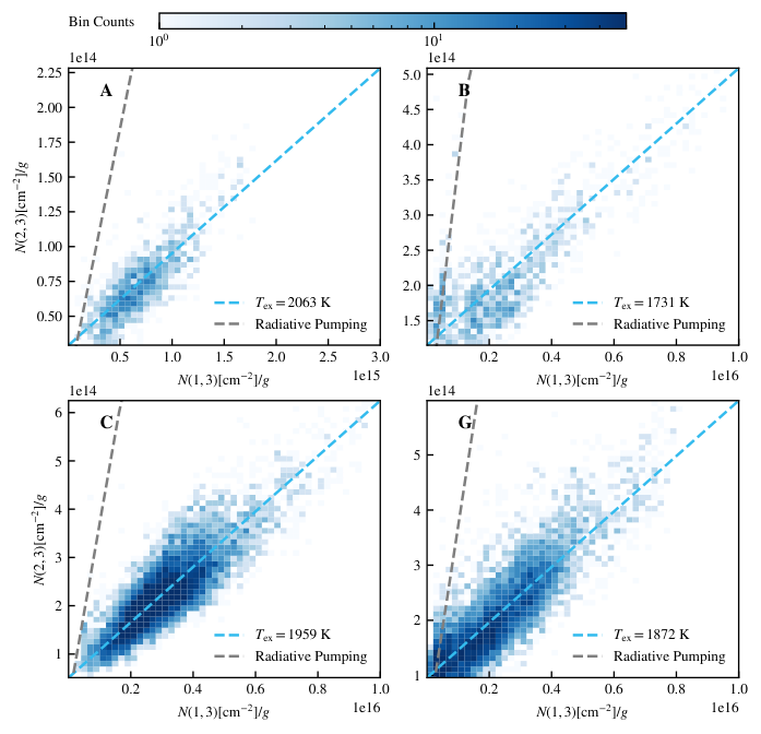
The emission of can be attributed to three main mechanisms: (1) being formed in the excited state on the grain surface (Hollenbach & McKee 1979, with a rate of cm s-1); (2) radiative pumping of the electronic lines followed by fluorescence; (3) inelastic collision with H, , and .
For dissociative J-type shocks, the molecules can be dissociated by the shocks but also reform rapidly in the post-shock cooling regions (Hollenbach & McKee 1989; Flower & Pineau Des Forêts 2010). Indeed, the re-formation pumping of can be the predominant mechanism in the fast shocks (Shinn et al. 2011; Shinn et al. 2012). However, the shocks propagated into the prominent molecular clumps are mostly slow and non-dissociative C-/CJ- type shocks (Richter et al. 1995b; Shinn et al. 2011; Reach et al. 2019). For the thermal collision with H atom (Jacobs et al. 1967; Wilgenbus et al. 2000, - collisional dissociation has much smaller rates,), the collisional dissociation rate of computed by Dove & Mandy 1986 is
| (4) |
where is the temperature of the neutral gas. Even for the gas with K and cm-3, the dissociation time scale is yr, which is much longer than the age of this SNR.
The non-detection of Br line (Burton et al. 1988, see Section 3.1.2, ) suggests the shock ionization is weak in these molecular clumps. We therefore do not expect a fast ionizing shock or a strong UV field.
Qualitatively, radiative pumping leads to cascades through excited vibrational and rotational levels of , which would efficiently form lines of the comparable population on vibrational levels higher than . Therefore, in Figure 12 we show the column density distributions of on , level (denote as level ) versus , level (as level ). The slope of this map can be used to derive the apparent excitation temperature,
| (5) |
where is the Boltzmann constant, is the apparent excitation temperature, , , and are column density, rotational degeneracy, and energy of populated on energy level , respectively. We fit the observed data with a straight line with a least-square fitting and plot it in blue (see Figure 12).
In all four regions, the apparent excitation temperature K. The slope of in Equation 5 should be for the radiative pumping dominant case, which could occur below the critical density of cm-3(Sternberg & Dalgarno 1989). This slope is much larger than the fitting result () in these four regions. The grey lines with a slope of 0.37 are plotted as an approximation of the radiative pumping dominant excitation process. Thus, both formation pumping and radiative pumping could be negligible in our regions.
In conclusion, collisional excitation is likely to be the dominant mechanism for exciting the K levels of in these dense molecular clumps with non-dissociative shocks. We will re-examine this from excitation temperature in the next section.
4.2 Comparison with pure rotational transitions in the literature
The pure rotational transitions have lower energy levels than the ro-vibrational transitions detected with VLT/KMOS. Mid-infrared observations based on space observatories, e.g., Neufeld et al. 2007 and Cesarsky et al. 1999, have detected (from 0-0 S(0) to S(7)) in region C with Spitzer IRS and (from 0-0 S(2) to S(7)) in region G with the Infrared Space Observatory (ISO)CAM, respectively. Here, we combine our new data with these mid-infrared data in regions C and G and plot population diagrams (Figure 13) with a very wide energy range from 509.9 K to 19085.8 K.
First, we correct the mid-infrared data with the same extinction adopted in this work. For clump C, Neufeld et al. 2007 present a Gaussian weighted average spectrum within a circular region centred at (06:17:42,22:21:29), with a HPBW of 25′′. This subregion contains the molecular clump in region C and knot Cc1, as labeled with the white circle in Figure 9 top panel. We extract the spectrum from our data with the same Gaussian weighting, which is plotted in the left panel of Figure 13. For region G, the ISOCAM data is compared with the spectrum extracted from an 18 region at “Peak B” in Cesarsky et al. 1999, as labeled with the white square in Figure 10 left panel. The population diagram is present in the right panel of Figure 13.
In both regions, the population diagrams have three vibrational levels, namely , , and , respectively. Only one data point exists for data at each region, so we overplot it in the figure without any fitting. The data points in all vibrational levels follow relatively straight lines, with different slopes. The slopes tend to flatten at high levels because of the presence of temperature gradients and multiple temperature components. Following the method presented in Section 3.2, we derive the and by fitting the lowest levels at the branch and plot the LTE population of the fitting results as the red lines in Figure 13. The flattening of the slope can be found by comparing the levels with the red lines.
In C-type shocks, the shock transition of temperature is continuous from K to K succeeding with radiative cooling. Such temperature gradients result in that the hotter gas with a smaller column density dominates the excitation of high energy states, while the cooler gas with a larger column density dominates that of the low energy states. Thus, as an integration in the line of sight, the apparent excitation temperatures of the higher energy levels can be larger than that of the lower levels but their column densities are orders of magnitudes smaller. The temperature and column density derived from the low levels represent the majority of the molecular gas involved in the shock transition which perhaps includes a wide precursor, and those derived from the low levels can represent the gas in the K warm shock layers (see also Section 4.3.3).
The temperature obtained with the above method can also be regarded as the rotational excitation temperature of level, hereafter . Similarly, we can derive and to present the rotational excitation on a specific vibrational level. Meanwhile, the vibrational temperatures between and levels are simply derived by
| (6) |
The derived rotational and vibrational excitation temperatures are marked in Figure 13. The vibrational temperatures and at the levels are consistent with the rotational temperatures and , respectively. This result suggests that the rotational and vibrational excitation should undergo the same mechanism, as we discussed in Section 4.1, collisional excitation.
The population diagrams of different v levels are not fully consistent with each other: at similar , the levels are more populated than the levels and the levels are also more populated than the levels. These features imply that the population diagrams can not be fully reproduced by simply combining multiple LTE components with different , and , which could be feasible when modeling the OMC-1 (Rousselot et al. 2000). Shinn et al. 2011 have successfully reproduced the level population of shocked in IC 443 C and G using the combination of two power-law thermal admixture models which assume that the column density in the C-shock is related to the temperature as .
It is worth noting that the branch shows the flattest trend which leads to the highest temperature and lowest column density among all vibrational levels, while branch has only moderate excitation temperature of K. The most reasonable explanation of the moderate temperature and column density derived from branch is that we only observed the lowest four levels while the slope can also flatten rapidly at higher levels. In fact, the flattening trend of the branch has appeared in the population diagram of region G (Figure 13 right). Fitting with only the lowest transitions would underestimate the temperature and overestimate column density.
Such population diagrams can also be found in the simulated shocks (Wrathmall et al. 2007; Nesterenok et al. 2019, e.g.) but it was not been interpreted in the literature. A detailed investigation needs the observations of more levels, whose ro-vibrational transitions, unfortunately, lie in the 1.87m opaque atmospheric band. Future James Webb Space Telescope observations can exhibit the most complete population diagrams and help the community with it.
4.3 Warm molecular gas in shocked regions
4.3.1 Multi-band comparison

In this section, we compare the multi-gas-phase distribution and excitation in the shock environment of IC 443, by comparing the data for our VLT/KMOS observations with multi-band ancillary data (Section 2.3) including JCMT CO 3-2 data, VLA & Arecibo H i 21-cm data, and the CFHT/SITELLE H/ZTF r band (which is dominated by the H emission) photometric data.
In Figure 14, the background colormap shows the H/ZTF r band images. The black contour shows the moment-0 map of high-velocity Hi ( km s-1). The white contour shows the moment-0 map of shocked CO =3-2 (both redshifted and blueshifted components from region G). The purple contour presents our KMOS 1-0 S(1) data.
The , high-velocity H i, and CO emission all show clumpy structures. All these species co-exist in the same regions, with peaks slightly staggered. On the other hand, the distribution of H seems more extended with filamentary structures. All emission is enclosed by CO and high-velocity H i emission. In A and B regions, H seems to have no spatial relation with the morphology, while in C and G regions, elongated H emission seems to be aligned with the structures with slight offsets.
4.3.2 Stratified shock structures
Region A exhibits the strongest H emission among all four regions, composed with several expanding shell-like structures. The H i emission in region A is enclosed by the H shell in the south. The clump (our FOVs) is on the ridge of the H i structure along the north-south direction. The spatial overlapping of H, Hi, , and [Fe ii] (Section 3.1.3) implies that the shock waves are propagating along the line of sight and interacting with the rarefied atomic gas and dense clump successively.
As Section 3.1.3 mentioned, region A shows strongly broaden [Fe ii] emission from the same region of the emission. To produce the [Fe ii] lines, it requires a fast shock with a velocity 50 to release Fe locked in the grain (Jones et al. 1994; Draine 1995). The observed broad velocity profile of [Fe ii] is consistent with the fast shock scenario. Therefore, we propose that in region A the shock still keeps its high velocity, either because the molecular clump here is intrinsically rarefied, or because it only recently starts to interact with the dense molecular clumps and produces emission. On the contrary, the shocks have been significantly decelerated by the dense molecular clumps in regions B, C, and G, which all show bright emission and weak [Fe ii] emission.
If the foreground gas is rarefied, the ISM in region A can be dissociated or ionized to H i and , and the grain can release Fe into gas. However, the detection of HCO+(Dickman et al. 1992), which has a high critical density , needs the existence of high-volume-density gas.
If the foreground gas is stratified with dense cores in the centre, the fast shock can still heat up surrounding diffuse gas, producing high-velocity H i, , and [Fe ii] lines. The central core part of the MC is still undisturbed. This scenario would expect a velocity difference among all these lines: . From Fig 6, the linewidth of [Fe ii] is larger than that of the lines. So we would be inclined to this case. Future high-velocity resolution observations could be useful to fully test these two scenarios.
In regions B, C, and G, H emission is much weaker than that in region A. The morphologies of H in these regions are more extended, often appearing only on one side of the molecular clumps.
Similar to region A, shock waves in regions B and C are also propagating along the line of sight. Our JCMT data and Zhang et al. 2010 show a strong 12CO clump in regions B and C, with 13CO emission, indicating the existence of a concentration of dense molecular gas. This distribution of atomic and molecular gas is interpreted by a schematic diagram of the molecular clump in region B proposed by Zhang et al. 2010, where the ionized and atomic gas in the outer layer of molecular clouds are accelerated and ablated by the fast shocks. The CO and emissions mainly come from the dense core surrounded by H i. The temperature and column density distribution shown in Figure 8 also support this scenario, where the dense gas is surrounded by the rarefied hot gas.
In region G, the shocks propagate perpendicular to the line of sight. The and CO clumps show spatially coexisting structures, while the H emission only appears at the east of the molecular clump. This can also be interpreted by a similar shock disturbance scheme as the vertical line of sight case.
Such a scenario is also similar to a classic astrophysical hydrodynamics test problem, the blob test (Agertz et al. 2007; Hopkins 2015, e.g.), where a spherical, dense, and cold cloud in the pressure equilibrium with a uniform rarefied, warm background gas is disrupted by a supersonic wind. Hydrodynamic simulations have shown that the ram-pressure ablates and disrupts the clouds with a complicated mixture of the Kelvin-Helmholtz instabilities (KHIs) and the Rayleigh-Taylor instabilities (Chandrasekhar 1961, RTIs) developing from the front of the cloud during the stripping. The KHIs and RTIs fragment the cloud into several small dense clumps and filaments with tails before the cloud finally being destructed (Hopkins 2015, e.g. see Section 4.4.3 and Figure 24 of).
The hierarchical structures of embedded knots and filaments we observed in the shocked warm emission regions (Section 3.1.1) can be the realistic astrophysical counterpart of such a disrupting cloud. The filamentary H emission, surrounding the molecular clumps, can be regarded as the ablated filaments and tails. Under such a cloud-fragmentation scenario, the CO and counterparts of the small bright knots can be tested with high-resolution sub-millimetre observations.
4.3.3 How much does the warm contribute in shocked regions?
Our detected - and - band lines mostly correspond to the high-volume-density component in the power-law thermal admixture model (Shinn et al. 2011). In the region G , we have obtained column density of the warm trunk is cm-2 and hardly reaches cm-2 (see Section 3.2.1).
In the same region G, Dell’Ova
et al. 2020 obtained the total
column density of shocked to be
cm-2 using the standard CO/
abundance ratio (), which is plausible to be adopted even in these
shocked clumps (van
Dishoeck et al. 1993). Comparing results from both
population diagrams of CO lines and the Large Velocity Gradient (LVG) method
with the expanding spherical geometry in the RADEX code
(van der Tak
et al. 2007). Dell’Ova
et al. 2020 find that column
density of shocked high-velocity CO is three times more than that obtained from
population diagrams.
This suggests that the warm molecular hydrogen with temperature K contributes to less than 1% of the total mass of the shocked .
4.4 Emission line contribution to 2MASS and bands
The Two Micron All-Sky Survey (Skrutskie et al. 2006, 2MASS; ) database has been widely used to provide the near-IR photometry of IC 443 and other SNRs in the bands (Rho et al. 2001; Su et al. 2014; Rho et al. 2003, e.g.). Using the HK grating, our KMOS observations cover the 2MASS ( m) band and ( m) band simultaneously and therefore provide an opportunity to measure contributions from lines.
Extended emission at band is often thought to be dominated by 1-0 S(1) 2.1218 m, which is actually quite strong in our observed fields. However, all the four strongest transitions (from 1-0 S(0) to S(3)) lay in the band. In fact, 1-0 (from S(0) to S(3)), 2-1 (S(5) to S(0)), and 3-2 (from S(1) to S(5)) could contribute to the flux of band, though we did not detect 3-2 S(4) and S(2) in any region. Also, in molecular shock regions like IC 443 A, B, C, and G here, the band images can also be dominant by ro-vibrational line emission.
To get a representative view, we extract a spatially-averaged spectrum from region C, where the emission almost distributes all over the FoV (Figure 3), and normalize to the flux of 1-0 S(1) line (Figure 15 black line). Then we convolve it with 2MASS and relative spectral response (RSR) (Cohen et al. 2003, Figure 15 green and red lines). The output spectrum is plotted in the light blue line in Figure 15. All lines with contribution larger than 1% of 1-0 S(1) are labeled in the figure.
In the band, the main components are 1-0 (from S(6) to S(9)) transitions, with 1-0 S(7) being the strongest one. In the band, the 1-0 S(1) transition is the strongest one, while the 1-0 S(2), 1-0 S(0), and 2-1 S(1) transitions contribute at similar levels. The 2-1 S(3) and S(2), 3-2 S(3) transitions also contribute a non-negligible part in the band. Although the 1-0 S(3) transition is almost as strong as 1-0 S(1), it seems to be attenuated by the low bandpass at the edge.
4.5 Young stellar object candidates in region G
With spectroscopic information from VLT/KMOS, we could identify the young stellar object (YSO) candidates selected by Dell’Ova et al. 2020. Six of the 65 YSO candidates selected from the ALLWISE catalog and one of their 79 YSO candidates selected from the 2MASS catalog are in the coverage of the G Region. These seven candidates are marked in Figure 10 left panel with white (WISE) and grey (2MASS) circles.
All these seven YSO candidates were classified as Class-I YSO. From the spectral indices derived by Dell’Ova et al. 2020, we can infer these sources should have a significant flux in band, on the order of erg s-1 cm-2 Å-1, which could be detected with our sensitivity.
To mock the aperture photometry conducted by WISE/2MASS, we extract the spectra of these targets by apertures with a diameter of two times the FWHM, and then we use rings with to evaluate and subtract the background. The FWHMs are for WISE W2 and for 2MASS images, respectively. In Figure 16, the black lines show the extracted spectra and the orange dashed lines show the continuum of these YSO candidates extrapolated from their WISE or 2MASS photometric SED and spectral index. The increasing continuum beginning from 2.2 m is the residuals of molecular emission from the lower atmosphere.
Among them, 2MASS J061643.13+223301.4 overlaps with a star which has a continuum spectrum. The last row of panels shows that the predicted continuum is consistent with the observed value. WISE J061643.22+223302.2 is only 1.5′′ away from this star, so a similar continuum spectrum can also be found in the fifth-row panels.
J061642.28+223241.6 is unfortunately located at the edge of our broken IFU, with one-fourth of the aperture without data. The other three-fourth aperture only has ro-vibrational lines without any continuum contribution.
All other YSO candidates do not show any continuum in the spectra. Even though we conducted ring-area background subtraction, we still found strong nebular emission lines in these spectra. J061642.91+223215.9 and J061643.87+223250.1 are located in two bright clumps. J061642.44+223206.3 and J061643.64+223232.1 also show strong emission, and they are only 3.9′′ and 2.1′′ away from two of the brightest clumps in this FOV, respectively.
We further cross-match the star overlapped with 2MASS J061643.12+223301.4 in Gaia eDR3 (Gaia Collaboration et al. 2021) and LAMOST DR7 (Luo et al. 2015) catalogues to check whether it is a young star. We find one star in a cone of radius 1′′ and no other stars are found within a cone of radius 5′′.
This star has a G magnitude of 16.663 mag, BP-G of 0.726, and G-RP of 0.830. The parallax in the Gaia catalogue is mas, and the geometric distance is pc (Bailer-Jones et al. 2021), similar to the distance of IC 443 ( pc). LAMOST observed this star twice on 21 Nov. 2014 and 21 Jan. 2015, respectively. The spectral type and star parameters including surface gravity , and effect temperature obtained in these two shots are consistent with each other, while the metallicity [Fe/H] has a large difference. These observed stellar parameters are summarised in Table 3.
If there is any physical connection between this star and SNR
IC 443, this star should be young.
We use the Bayesian stellar parameter estimator PARAM 1.5 44
4
http://stev.oapd.inaf.it/cgi-bin/param
(da Silva
et al. 2006) and adopt PARSEC (Bressan
et al. 2012)
stellar models to estimate the age of this star with Gaia and LAMOST data. The
most probable ages are Gyr and
Gyr for the LAMOST 2014 and 2015 data, respectively.
This is much older than the progenitor of IC 443, thus it is unlikely to be connected with IC 443 and its progenitor.
| g Mag. | BP-G | G-RP | Parallax (mas) | Distance (pc) | Class | [Fe/H] | Age (Gyr) | |||
|---|---|---|---|---|---|---|---|---|---|---|
| 2014 | 16.63 | 0.726 | 0.830 | G9 | ||||||
| 2015 | K3 |
In conclusion, in our observed fields, the majority of the YSO candidates selected from the 2MASS and WISE samples are not continuum sources and their broadband NIR and MIR images are dominated by the line emission. The only continuum source we observed is likely an old star whose IR spectrum is significantly contaminated by line emission as well.

5 Conclusions
With VLT/KMOS, we observed IC 443 A, B, C, and G, four regions with strong interaction between supernova shock waves and molecular clumps. Facilitated by the 8.2-m diameter mirror and near-infrared integral field spectroscopic instrument KMOS, our observations present twenty ro-vibrational lines, Br line, and two [Fe ii] lines in these regions.
The distribution of warm molecular hydrogen shows clumpy and hierarchical structures, with small bright knots that are embedded in the gas clumps. The molecular hydrogen emission is optically thin at the near-infrared band and is mainly excited by collisional processes.
We present the temperature and column density distribution maps and phase diagrams of these four regions derived by the population diagram method, find that the temperature and column density of these shocked warm ranges from K to K and from cm-2 to cm-2. These maps give us an intuitive knowledge about how warm molecular gas gets excited in shocked regions. They can also help us plan and analyze future multi-band observations zooming in these molecular clumps.
The extended line profile of [Fe II] 1.6440 m line is detected in region A, which supports that [Fe II] is more likely to come from the fast shock region where the grain can be sputtered. This also suggests that region A might be in the early phase of shock-molecular clump interaction when the shock waves haven’t been significantly decelerated yet.
We detect Br line in region A with an intensity of erg s-1 cm-2 arcsec-2 and give a the new upper limit of Br line emission in regions B, C, and G of erg s-1 cm-2 arcsec-2. Comparing with the H emission detected in these regions, we address questions about the states of the atomic hydrogen in these shocked molecular clumps.
We compare our data with optical, mid-infrared, and radio observations. The spatial distribution of different phases of gas reveals the shock structures. Comparing with the total column density of shocked , we find that shocked warm contributes to 1% mass of all the shocked .
Last, we verified YSO candidates in our Region G data and find no young stellar counterparts for all of them. The infrared emission of these YSO candidates is significantly contaminated by line emission. Cross-checking with spectroscopic observations thus becomes extremely important for such a YSO candidate census.
In the future, multi-band observations of various species in the multi-phase gas will be wrapped up and give a panchromatic perspective of shocked regions in IC 443. We have performed Arecibo, JVLA, and FAST observations with a spatial resolution higher than before. We have also proposed optical integral field observations with CFHT/SITTILE and large field optical lines narrowband image of IC 443, and the data will come soon. We also plan to propose high resolution () infrared spectroscopic observations with state-of-the-art telescopes and instruments like VLT/CRIRES+ or CFHT/SPIRou. These data will help us obtain a more comprehensive understanding of the stratification of ionization, dissociation structures, and kinematics of ionized gas, neutral gas, and hot molecular gas in shocked regions.
Acknowledgements
This work is based on observations collected at the European Southern Observatory under ESO programme 0104.C-0924(A). We thank Dr. Paola Popesso and colleagues from ESO Operation Helpdesk for their kind help and advice. YWD is grateful to Yichen Sun and Haochang Jiang for their useful discussions.
ZYZ and YWD acknowledge the support of the National Natural Science Foundation of China (NSFC) under grants No. 12041305, 12173016. ZYZ and YWD acknowledge the Program for Innovative Talents, Entrepreneur in Jiangsu. ZYZ and YWD acknowledge the science research grants from the China Manned Space Project with NO.CMS-CSST-2021-A08, NO.CMS-CSST-2021-A07. HL was supported by NASA through the NASA Hubble Fellowship grant HST-HF2-51438.001-A awarded by the Space Telescope Science Institute, which is operated by the Association of Universities for Research in Astronomy, Incorporated, under NASA contract NAS5-26555.
We use python packages NumPy (Harris
et al. 2020),
SciPy (Virtanen
et al. 2020), and Astropy
(Astropy
Collaboration et al. 2013; Astropy
Collaboration et al. 2018) to analyze the data cubes and
use Matplotlib (Hunter 2007) to visualisation. To remove the
stellar continuum, we use the widely used Astropy package
photutils to find and mask the stars.
Data Availability
The processed KMOS cubes can be accessed from ESO Science Portal55 5 http://archive.eso.org/scienceportal/home. The raw data and calibration frames of the KMOS observations are provided via the ESO archive facility66 6 http://archive.eso.org/eso/eso_archive_main.html.
References
- Agertz et al. (2007) Agertz O., et al., 2007, MNRAS, 380, 963
- Astropy Collaboration et al. (2013) Astropy Collaboration et al., 2013, A&A, 558, A33
- Astropy Collaboration et al. (2018) Astropy Collaboration et al., 2018, AJ, 156, 123
- Bailer-Jones et al. (2021) Bailer-Jones C. A. L., Rybizki J., Fouesneau M., Demleitner M., Andrae R., 2021, AJ, 161, 147
- Bressan et al. (2012) Bressan A., Marigo P., Girardi L., Salasnich B., Dal Cero C., Rubele S., Nanni A., 2012, MNRAS, 427, 127
- Buckle et al. (2009) Buckle J. V., et al., 2009, MNRAS, 399, 1026
- Burton et al. (1988) Burton M. G., Geballe T. R., Brand P. W. J. L., Webster A. S., 1988, MNRAS, 231, 617
- Cappellari & Copin (2003) Cappellari M., Copin Y., 2003, MNRAS, 342, 345
- Cardelli et al. (1989) Cardelli J. A., Clayton G. C., Mathis J. S., 1989, ApJ, 345, 245
- Carpenter et al. (1995) Carpenter J. M., Snell R. L., Schloerb F. P., 1995, ApJ, 445, 246
- Cesarsky et al. (1999) Cesarsky D., Cox P., Pineau des Forêts G., van Dishoeck E. F., Boulanger F., Wright C. M., 1999, A&A, 348, 945
- Chandrasekhar (1961) Chandrasekhar S., 1961, Hydrodynamic and hydromagnetic stability
- Chevalier (1999) Chevalier R. A., 1999, ApJ, 511, 798
- Cohen et al. (2003) Cohen M., Wheaton W. A., Megeath S. T., 2003, AJ, 126, 1090
- Davies et al. (2013) Davies R. I., et al., 2013, A&A, 558, A56
- Dekel et al. (2019) Dekel A., Sarkar K. C., Jiang F., Bournaud F., Krumholz M. R., Ceverino D., Primack J. R., 2019, MNRAS, 488, 4753
- Dell’Ova et al. (2020) Dell’Ova P., et al., 2020, A&A, 644, A64
- Denoyer (1979) Denoyer L. K., 1979, ApJ, 232, L165
- Dickman et al. (1992) Dickman R. L., Snell R. L., Ziurys L. M., Huang Y.-L., 1992, ApJ, 400, 203
- Dove & Mandy (1986) Dove J. E., Mandy M. E., 1986, ApJ, 311, L93
- Draine (1995) Draine B. T., 1995, Ap&SS, 233, 111
- Draine & McKee (1993) Draine B. T., McKee C. F., 1993, ARA&A, 31, 373
- Drissen et al. (2019) Drissen L., et al., 2019, MNRAS, 485, 3930
- Fesen & Kirshner (1980) Fesen R. A., Kirshner R. P., 1980, ApJ, 242, 1023
- Flower & Pineau Des Forêts (2010) Flower D. R., Pineau Des Forêts G., 2010, MNRAS, 406, 1745
- Freudling et al. (2013) Freudling W., Romaniello M., Bramich D. M., Ballester P., Forchi V., García-Dabló C. E., Moehler S., Neeser M. J., 2013, A&A, 559, A96
- Gaia Collaboration et al. (2021) Gaia Collaboration et al., 2021, A&A, 649, A1
- Goldsmith & Langer (1999) Goldsmith P. F., Langer W. D., 1999, ApJ, 517, 209
- Harris et al. (2020) Harris C. R., et al., 2020, Nature, 585, 357
- Hollenbach & McKee (1979) Hollenbach D., McKee C. F., 1979, ApJS, 41, 555
- Hollenbach & McKee (1989) Hollenbach D., McKee C. F., 1989, ApJ, 342, 306
- Hopkins (2015) Hopkins P. F., 2015, MNRAS, 450, 53
- Hopkins et al. (2014) Hopkins P. F., Kereš D., Oñorbe J., Faucher-Giguère C.-A., Quataert E., Murray N., Bullock J. S., 2014, MNRAS, 445, 581
- Huang et al. (1986) Huang Y. L., Dickman R. L., Snell R. L., 1986, ApJ, 302, L63
- Hunter (2007) Hunter J. D., 2007, Computing in Science & Engineering, 9, 90
- Ikeuchi et al. (1984) Ikeuchi S., Habe A., Tanaka Y. D., 1984, MNRAS, 207, 909
- Jacobs et al. (1967) Jacobs T. A., Giedt R. R., Cohen N., 1967, J. Chem. Phys., 47, 54
- Jones et al. (1994) Jones A. P., Tielens A. G. G. M., Hollenbach D. J., McKee C. F., 1994, ApJ, 433, 797
- Jones et al. (1998) Jones T. W., et al., 1998, PASP, 110, 125
- Koda et al. (2019) Koda J., Teuben P., Sawada T., Plunkett A., Fomalont E., 2019, PASP, 131, 054505
- Kokusho et al. (2020) Kokusho T., Torii H., Nagayama T., Kaneda H., Sano H., Ishihara D., Onaka T., 2020, ApJ, 899, 49
- Koo et al. (2016) Koo B.-C., Raymond J. C., Kim H.-J., 2016, Journal of Korean Astronomical Society, 49, 109
- Koo et al. (2020) Koo B.-C., Kim C.-G., Park S., Ostriker E. C., 2020, ApJ, 905, 35
- Krumholz et al. (2019) Krumholz M. R., McKee C. F., Bland-Hawthorn J., 2019, ARA&A, 57, 227
- Lada & Lada (2003) Lada C. J., Lada E. A., 2003, ARA&A, 41, 57
- Le Bourlot et al. (1999) Le Bourlot J., Pineau des Forêts G., Flower D. R., 1999, MNRAS, 305, 802
- Lee et al. (2008) Lee J.-J., Koo B.-C., Yun M. S., Stanimirović S., Heiles C., Heyer M., 2008, AJ, 135, 796
- Lee et al. (2012) Lee J.-J., Koo B.-C., Snell R. L., Yun M. S., Heyer M. H., Burton M. G., 2012, ApJ, 749, 34
- Lehmann et al. (2020) Lehmann A., Godard B., Pineau des Forêts G., Falgarone E., 2020, A&A, 643, A101
- Leonidaki et al. (2013) Leonidaki I., Boumis P., Zezas A., 2013, MNRAS, 429, 189
- Luo et al. (2015) Luo A. L., et al., 2015, Research in Astronomy and Astrophysics, 15, 1095
- Mangum & Shirley (2015) Mangum J. G., Shirley Y. L., 2015, PASP, 127, 266
- Masci et al. (2019) Masci F. J., et al., 2019, PASP, 131, 018003
- McKee & Hollenbach (1980) McKee C. F., Hollenbach D. J., 1980, ARA&A, 18, 219
- McMullin et al. (2007) McMullin J. P., Waters B., Schiebel D., Young W., Golap K., 2007, in Shaw R. A., Hill F., Bell D. J., eds, Astronomical Society of the Pacific Conference Series Vol. 376, Astronomical Data Analysis Software and Systems XVI. p. 127
- Nesterenok et al. (2019) Nesterenok A. V., Bossion D., Scribano Y., Lique F., 2019, MNRAS, 489, 4520
- Neufeld et al. (2007) Neufeld D. A., Hollenbach D. J., Kaufman M. J., Snell R. L., Melnick G. J., Bergin E. A., Sonnentrucker P., 2007, ApJ, 664, 890
- Olbert et al. (2001) Olbert C. M., Clearfield C. R., Williams N. E., Keohane J. W., Frail D. A., 2001, ApJ, 554, L205
- Peek et al. (2011) Peek J. E. G., et al., 2011, ApJS, 194, 20
- Popovas & Jørgensen (2016) Popovas A., Jørgensen U. G., 2016, A&A, 595, A130
- Reach et al. (2019) Reach W. T., Tram L. N., Richter M., Gusdorf A., DeWitt C., 2019, ApJ, 884, 81
- Rho & Petre (1998) Rho J., Petre R., 1998, ApJ, 503, L167
- Rho et al. (2001) Rho J., Jarrett T. H., Cutri R. M., Reach W. T., 2001, ApJ, 547, 885
- Rho et al. (2003) Rho J., Reynolds S. P., Reach W. T., Jarrett T. H., Allen G. E., Wilson J. C., 2003, ApJ, 592, 299
- Richter et al. (1995a) Richter M. J., Graham J. R., Wright G. S., Kelly D. M., Lacy J. H., 1995a, ApJ, 449, L83
- Richter et al. (1995b) Richter M. J., Graham J. R., Wright G. S., 1995b, ApJ, 454, 277
- Roueff et al. (2019) Roueff E., Abgrall H., Czachorowski P., Pachucki K., Puchalski M., Komasa J., 2019, A&A, 630, A58
- Rousselot et al. (2000) Rousselot P., Lidman C., Cuby J. G., Moreels G., Monnet G., 2000, A&A, 354, 1134
- Sharples et al. (2013) Sharples R., et al., 2013, The Messenger, 151, 21
- Shinn et al. (2011) Shinn J.-H., Koo B.-C., Seon K.-I., Lee H.-G., 2011, ApJ, 732, 124
- Shinn et al. (2012) Shinn J.-H., Lee H.-G., Moon D.-S., 2012, ApJ, 759, 34
- Skrutskie et al. (2006) Skrutskie M. F., et al., 2006, AJ, 131, 1163
- Snell et al. (2005) Snell R. L., Hollenbach D., Howe J. E., Neufeld D. A., Kaufman M. J., Melnick G. J., Bergin E. A., Wang Z., 2005, ApJ, 620, 758
- Sternberg & Dalgarno (1989) Sternberg A., Dalgarno A., 1989, ApJ, 338, 197
- Su et al. (2014) Su Y., Fang M., Yang J., Zhou P., Chen Y., 2014, ApJ, 788, 122
- Troja et al. (2008) Troja E., Bocchino F., Miceli M., Reale F., 2008, A&A, 485, 777
- Virtanen et al. (2020) Virtanen P., et al., 2020, Nature Methods, 17, 261
- Wang & Scoville (1992) Wang Z., Scoville N. Z., 1992, ApJ, 386, 158
- Wilgenbus et al. (2000) Wilgenbus D., Cabrit S., Pineau des Forêts G., Flower D. R., 2000, A&A, 356, 1010
- Wrathmall et al. (2007) Wrathmall S. A., Gusdorf A., Flower D. R., 2007, MNRAS, 382, 133
- Wright et al. (2010) Wright E. L., et al., 2010, AJ, 140, 1868
- Xu et al. (2011) Xu J.-L., Wang J.-J., Miller M., 2011, ApJ, 727, 81
- Zhang et al. (2010) Zhang Z., Gao Y., Wang J., 2010, Science China Physics, Mechanics, and Astronomy, 53, 1357
- Zucker et al. (2020) Zucker C., Speagle J. S., Schlafly E. F., Green G. M., Finkbeiner D. P., Goodman A., Alves J., 2020, A&A, 633, A51
- da Silva et al. (2006) da Silva L., et al., 2006, A&A, 458, 609
- van Dishoeck et al. (1993) van Dishoeck E. F., Jansen D. J., Phillips T. G., 1993, A&A, 279, 541
- van der Tak et al. (2007) van der Tak F. F. S., Black J. H., Schöier F. L., Jansen D. J., van Dishoeck E. F., 2007, A&A, 468, 627
Appendix A Atmospheric radiance in KMOS HK band
The radiance residuals (mainly OH sky lines) are difficult to perfectly subtracted from the spectra. Figure 17 presents the atmospheric radiance spectrum in KMOS HK band at Paranal with PWV=3.5 obtained from the ESO SkyCalc as a reference.
Appendix B Small Bright Knots
Here we list the detected lines (Table 4) in the ten small bright knots.
| Transition | (m) | (K) | Line Intensity ( erg s-1 cm-2 sec-2) | |||||||||
|---|---|---|---|---|---|---|---|---|---|---|---|---|
| Ac1 | Ac2 | Bc1 | Bc2 | Cc1 | Cc2 | Gc1 | Gc2 | Gc3 | Gc4 | |||
| 1-0 S(11) | 1.6504 | 18979.1 | … | … | … | … | 0.10 | 0.26 | … | … | … | … |
| 1-0 S(10) | 1.6665 | 17310.8 | 0.12 | 0.10 | … | … | 0.14 | 0.29 | … | … | … | 0.37 |
| 1-0 S(9) | 1.6877 | 15721.5 | 0.61 | 0.79 | 0.48 | 0.72 | 1.07 | 1.99 | 1.27 | 0.79 | 0.97 | 0.84 |
| 1-0 S(8) | 1.7147 | 14220.5 | 0.40 | 0.55 | 0.40 | 0.56 | 0.65 | 1.28 | … | 0.72 | 0.90 | 0.57 |
| 1-0 S(7) | 1.7480 | 12817.3 | 2.10 | 2.90 | 2.35 | 3.46 | 4.15 | 7.31 | 4.40 | 4.50 | 3.90 | 2.78 |
| 1-0 S(6) | 1.7880 | 11521.1 | 1.12 | 1.53 | 1.41 | 2.16 | 2.19 | 4.06 | 2.71 | 2.83 | 2.03 | 1.54 |
| 1-0 S(5)* | 1.8358 | 10341.2 | 0.13 | 0.32 | 0.30 | 1.13 | 0.11 | 0.37 | … | 0.05 | 0.10 | … |
| 1-0 S(4)* | 1.8919 | 9286.4 | 0.08 | 0.21 | 0.39 | 1.22 | 0.21 | 0.45 | 0.16 | … | 0.09 | … |
| 1-0 S(3)* | 1.9576 | 8364.9 | 11.86 | 18.61 | 14.37 | 18.74 | 24.11 | 32.88 | 17.82 | 24.67 | 21.12 | 16.64 |
| 1-0 S(2) | 2.0338 | 7584.3 | 3.23 | 4.54 | 6.55 | 9.47 | 8.43 | 11.45 | 8.23 | 8.43 | 7.40 | 5.22 |
| 1-0 S(1) | 2.1218 | 6951.3 | 8.85 | 12.39 | 19.71 | 27.94 | 24.32 | 31.40 | 23.65 | 24.54 | 21.05 | 15.50 |
| 1-0 S(0) | 2.2233 | 6471.4 | 2.10 | 2.89 | 4.91 | 6.73 | 5.80 | 7.06 | 5.80 | 5.81 | 5.01 | 3.64 |
| 2-1 S(5)* | 1.9449 | 15762.7 | … | … | 0.13 | 0.29 | 0.06 | 0.12 | 0.07 | 0.08 | 0.05 | … |
| 2-1 S(4)* | 2.0041 | 14763.5 | … | 0.51 | 0.37 | 0.38 | … | 0.30 | 1.27 | … | 0.57 | … |
| 2-1 S(3) | 2.0735 | 13890.2 | 0.52 | 0.90 | 1.18 | 1.49 | 1.31 | 2.38 | 2.38 | 2.21 | 1.63 | 0.93 |
| 2-1 S(2) | 2.1542 | 13150.3 | 0.40 | 0.54 | 0.59 | 0.73 | 0.74 | 1.17 | 0.75 | 0.76 | 0.70 | 0.46 |
| 2-1 S(1) | 2.2477 | 12550.0 | 1.10 | 1.62 | 1.72 | 2.30 | 2.38 | 3.56 | 2.29 | 2.44 | 2.42 | 1.46 |
| 2-1 S(0) | 2.3556 | 12094.9 | 0.95 | 0.48 | 0.62 | 0.70 | 0.67 | 1.02 | 0.38 | 0.64 | 0.71 | 0.76 |
| 3-2 S(5) | 2.0656 | 20855.7 | … | 0.23 | … | … | 0.20 | … | … | 0.17 | 0.27 | 0.10 |
| 3-2 S(3) | 2.2014 | 19085.8 | 0.25 | 0.43 | 0.35 | 0.30 | 0.57 | 0.94 | 0.43 | 0.42 | 0.57 | 0.39 |
| ∗ These lines are attenuated by the atmospheric absorption. Their intensities are likely underestimated. | ||||||||||||