Exploring the Advantages of Quantum Generative Adversarial Networks in Generative Chemistry
Abstract
De novo drug design with desired biological activities is crucial for developing novel therapeutics for patients. The drug development process is time and resource-consuming, and it has a low probability of success. Recent advances in machine learning and deep learning technology have reduced the time and cost of the discovery process and therefore, improved pharmaceutical research and development. In this paper, we explore the combination of two rapidly-developing fields with lead candidate discovery in the drug development process. First, Artificial intelligence has already been demonstrated to successfully accelerate conventional drug design approaches. Second, quantum computing has demonstrated promising potential in different applications, such as quantum chemistry, combinatorial optimizations, and machine learning. This manuscript explores hybrid quantum-classical generative adversarial networks (GAN) for small molecule discovery. We substituted each element of GAN with a variational quantum circuit (VQC) and demonstrated the quantum advantages in the small drug discovery. Utilizing a VQC in the noise generator of a GAN to generate small molecules achieves better physicochemical properties and performance in the goal-directed benchmark than the classical counterpart. Moreover, we demonstrate the potential of a VQC with only tens of learnable parameters in the generator of GAN to generate small molecules. We also demonstrate the quantum advantage of a VQC in the discriminator of GAN. In this hybrid model, the number of learnable parameters is significantly less than the classical ones, and it can still generate valid molecules. The hybrid model with only tens of training parameters in the quantum discriminator outperforms the MLP-based one in terms of both generated molecule properties and the achieved KL divergence.
I Introduction
The drug development process includes discovery and development, pre-clinical research, clinical research, Food and Drug Administration (FDA) review, and FDA post-market safe monitoring. The entire process is time and resource-consuming and has a low probability of success with approximately 4% of pre-clinical drugs eventually granted license Hingorani et al. 2019. The average time for a new medicine to complete the journey from initial discovery to the marketplace takes at least ten years Abreu 2020. The estimated median capitalized research and design (R&D) cost per new drug (accounting for the cost of failures) was $985 million between 2009 and 2018 Wouters et al. 2020. Recent advances in machine learning and deep learning technology have improved and reduced the cost of pharmaceutical R&D Aliper et al. 2016; Kadurin et al. 2017a; Zhavoronkov 2018; Carracedo-Reboredo et al. 2021; Kao et al. 2021; Kolluri et al. 2022. For example, some of us Zhavoronkov et al. 2019 discovered potent inhibitors of discoidin domain receptor 1 (DDR1), a kinase target implicated in fibrosis and other diseases, in 21 days. Chan et al. Chan et al. 2019 estimated their machine learning algorithms would shrink the drug candidate identification phase from a few months to one year.
De novo drug design refers to a novel chemical compound design with desired pharmacological and physicochemical properties Schneider and Fechner 2005. The discovery of novel chemical compounds with desired biological activities is a critical step to keep the drug discovery pipeline moving forward Fischer et al. 2019. It is also crucial for developing novel therapeutics for patients Mouchlis et al. 2021. Conventional approaches include ligand-based drug design (LBDD), fragment-based drug design (FBDD), and structure-based drug design (SBDD). LBDD is based on known active binders of a biological target, and FBDD identifies small molecular fragments with weak affinity for a biomolecular target of interest and assembles them into fully drug-like compounds Speck-Planche 2018. Aside from LBDD and FBDD, SBDD is based on the properties of the active site of a biological target.
Artificial intelligence (AI) has made a breakthrough in the recent de novo molecule design Mamoshina et al. 2018; Zhavoronkov et al. 2020; Paul et al. 2021. We identify four well-known generative machine learning algorithms in the field: evolutionary algorithms (EA), recurrent neural network (RNN) such as gated recurrent unit (GRU) and long short-term memory (LSTM), autoencoders such as adversarial autoencoder (AAE) and variational autoencoder (VAE), and generative adversarial network (GAN) Martinelli 2022. GAN Goodfellow et al. 2014 has become a popular network architecture for generating highly realistic data Karras et al. 2017, and it has shown remarkable results for generating data that mimics a data distribution in different tasks Isola et al. 2017; Zhu et al. 2017; Karras et al. 2019; Jangid et al. 2022. GAN consists of a generator and a discriminator defined by an artificial neural network (ANN). The parameters of a GAN can be learned by backpropagation. The generator takes random noises as input and tries to imitate the data distribution, and the discriminator tries to distinguish between the fake and real samples. A GAN is trained until the discriminator cannot distinguish the generated data from the real data.
GANs are one of the most successful generative models in the drug discovery field, and several different GAN architectures have been proposed in the past decades in de novo drug discovery Kadurin et al. 2017b; Vanhaelen et al. 2020; Xu et al. 2021. Zhavoronkov et al. Zhavoronkov et al. 2019 proposed a deep generative model called generative tensorial reinforcement learning (GENTRL) for de novo small molecule generation. The GENTRL generates novel drugs with better synthetic feasibility and biological activity. Guimaraes et al. Guimaraes et al. 2017 proposed an objective-reinforced generative adversarial network (ORGAN) that combines the GAN and reinforcement learning (RL) algorithm. ORGAN is built on SeqGAN Yu et al. 2017 and is the first GAN architecture in the de novo molecule generation. It is a sequential generative model operating on simplified molecular-input line-entry system (SMILES) string representations of molecules. The generated samples of ORGAN maintain information originally learned from data, retain sample diversity, and show improvement in the desired drug properties. Prykhodko et al. Prykhodko et al. 2019 presented a novel neural network architecture called LatentGAN for de novo molecular design. It combines an autoencoder and a generative adversarial neural network. The generator and discriminator of LatentGAN take -dimensional vectors as inputs. These inputs derived from the code layer of an autoencoder are trained as a SMILES heteroencoder Kotsias et al. 2020. This method allows LatentGAN to focus on optimizing the sampling without worrying about SMILES syntax issues. Cao and Kipf introduced MolGAN De Cao and Kipf 2018 for small molecule de novo design which operates directly on graph-structured data. It is the first GAN to address the generation of graph-structured data in the context of molecular generation. MolGAN is demonstrated to generate close to 100% valid compounds in experiments on the quantum machines 9 (QM9) chemical database. The generated molecules of MolGAN have better chemical properties particularly in synthesizability and solubility than the generated compounds of ORGAN. Neither ORGAN nor MolGAN is directly compared with LatentGAN in the paper. These generative models have the potential to be improved with quantum machine learning algorithms.
AI-driven strategies have the potential to explore adjacent chemical space compared to classical discovery efforts in de novo drug design Jayatunga et al. 2022. However, the traditional generative machine learning algorithms have difficulty exploring the new chemical space different from the training dataset. The Hilbert space of the molecule scales exponentially with molecule size. It increases the difficulty for the classical generative model on sampling as the landscape becomes extremely large and impossible to screen all possible configurations. Thus, an efficient sampling method is needed.
The applications of quantum computing can be found in different fields, such as solving routing problems Neukart et al. 2017; Harwood et al. 2021, stock price forecasting Orus et al. 2019; Liu and Ma 2022, multi-task classification Du et al. 2022, two-player zero-sum game Yin et al. 2022, high-resolution handwritten digits generation Rudolph et al. 2022, the discovery of molecular properties Aspuru-Guzik et al. 2005; Lanyon et al. 2010; Peruzzo et al. 2014; O’Malley et al. 2016; Kandala et al. 2017; Cao et al. 2019; Quantum et al. 2020; Gao et al. 2021a, tautomeric state prediction Shee et al. 2022, and drug design Cao et al. 2018; Li et al. 2021. We can obtain more efficient and accurate results by utilizing the technique of quantum annealer, quantum machine learning, and quantum algorithm. These advantages that utilize the fundamental properties of quantum mechanics to achieve better performances compared to the classical methods are called quantum advantages. These performances can be on the computational resources requirement in simulation, computational efficiency in algorithm development, and measurement precision in metrology. More specifically, quantum advantages can be identified in three aspects: scalability, complexity, and accuracy. The idea of utilizing the intrinsic quantum properties of quantum processors to simulate quantum systems was proposed by Feynman in 1982 Feynman et al. 1982, allowing us to understand the characteristics of large quantum systems with a feasible computational resource and achieving the quantum advantage of scalability. For complexity, researchers found that the complexity of many algorithms Grover 1996; Coppersmith 2002; Shor 1994; Kitaev 1995 can be significantly reduced by the quantum properties. Better measurement accuracy can be achieved by sophisticated designed protocols that enhance the accuracy from the standard quantum limit to the Heisenberg limit Giovannetti et al. 2004; Giovannetti et al. 2006; Lloyd 2008; Komar et al. 2014
Although quantum computing seems to lead a significant leap in solving resource-demanding problems, a few challenges remain to be overcome, such as the imperfect reliability of the qubits prohibits the physical implementation of large-scale quantum computers Chao and Reichardt 2018. Nevertheless, noisy intermediate-scale quantum (NISQ) computers can still perform classical challenge tasks accompanied by quantum advantages Bharti et al. 2022. For example, the advantages are shown in sampling the output of a pseudo-random quantum circuit Arute et al. 2019, the sampling time complexity of a Torontonian of a matrix Zhong et al. 2020; Quesada et al. 2018, expressively in unsupervised learning Gao et al. 2021b, and parameter space complexity in reinforcement learning Chen et al. 2020.
Although the idea of data conversion in the quantum circuit through gate operators is similar to the classical neural network, efficient sampling that can be achieved by quantum circuits as the fundamental principle of quantum mechanics enables computational processes that are beyond what is possible on classical computers. Several studies have demonstrated that variational quantum circuit (VQC) Bharti et al. 2022 performs the advantages in expression power Du et al. 2020, learnability Du et al. 2021a, and robustness Du et al. 2021b. It indicates that VQC can greatly boost the solution to the problem, e.g., drug discovery, which is hard to tackle by the classical neural network. In addition, Blunt et al. Blunt et al. 2022 discuss that using the current best theoretical algorithms on a quantum computer would reduce the pharmaceutical R&D period from many years to only a week.
The innate advantages of VQC are suited for computational resource-demanding tasks, such as identifying possible chemical reaction pathways and predicting molecule structures. The ground state energy of different molecule configurations reveals the most plausible reaction mechanism. It is demonstrated that the ground state energy of small molecules, such as , LiH, Kandala et al. 2017, , and diazene Quantum et al. 2020, can be obtained by VQC, where the parameterized angles in the circuit are updated iteratively on the classical computer until the minimum energies are achieved under the given molecule configuration. Furthermore, the obtained ground state energies are shown to be consistent with the results from the classical Full-CI calculation Gao et al. 2021a. In addition, Gircha et al. Gircha et al. 2021 trained a discrete variational autoencoder (DVAE) for generative chemistry and drug design. Their model is small enough to fit an annealer and produce drug-like molecules.
Quantum generative adversarial network (QuGAN) Lloyd and Weedbrook 2018 provided the first theoretical framework of quantum adversarial learning. QuGAN’s exponential advantages over classical GANs directly result from the ability of quantum information processors to represent -dimensional features using qubits with a time complexity of . Recent studies also showed that generative models implemented by quantum circuits with fewer architectural complexities could easily bypass their classical counterparts Huang et al. 2021; Li et al. 2021. Dallaire-Demers et al. provided the first feasible implementation of QuGAN using quantum circuits in a simulator Dallaire-Demers and Killoran 2018. Analogous proposals of QuGAN for continuous functions have been proposed during the same period Romero and Aspuru-Guzik 2021. Later on, QuGANs demonstrated its first successful training on the MNIST dataset on a physical quantum device Huang et al. 2021. Li et al. Li et al. 2021 pushed the research to the real world further by showing the QuGANs can learn or generate the distribution of the QM9 dataset, which provides the quantum chemical properties for small organic molecules in drug design. However, the source code (https://github.com/jundeli/quantum-gan) they provided struggles with generating training-set-like molecules. In addition, it lacks a detailed comparison between the generated samples from QuGAN and those from classical GAN.
In this work, we perform the training tasks on the QM9 dataset using the classical and quantum GAN. We not only demonstrate that the quantum GAN outperforms the classical GAN in the drug properties of generated compounds and the goal-directed benchmark but ensure that the trained quantum GANs can generate training-set-like molecules by using the variational quantum circuit as the noise generator. In addition, we show the potential of the variational quantum circuit in the generator of GAN to generate small molecules. In the end, we demonstrate that the quantum discriminator of GAN outperforms the classical counterpart in terms of generated molecule properties and KL-divergence score. The source codes will be publicly available once this manuscript is accepted. In addition, the hybrid models are planned to be integrated into the Insilico Medicine Chemistry42TM Ivanenkov et al. 0 shortly.
II Methodology
Generative adversarial net (GAN) Goodfellow et al. 2014 was first proposed in 2014. It consists of two elements: a generator and a discriminator. The objective of the generator is to generate fake data which mimics the real training data, and the goal of the discriminator is to distinguish real data from fake data. To achieve these goals, the generator and discriminator are trained at the same time using the training data. During the training process, both elements compete with each other and iteratively improve with one another. By the end, the generator can generate novel data highly similar to the data from the training dataset. More details of GAN can be found in the original GAN Goodfellow et al. 2014 paper. Quantum generative adversarial networks (QuGANs) Dallaire-Demers and Killoran 2018; Lloyd and Weedbrook 2018 were first introduced around late July 2018. Dallaire-Demers and Killoran Dallaire-Demers and Killoran 2018 extended adversarial training to the quantum domain, built generative adversarial networks using quantum circuits, and demonstrated that QuGANs can be trained successfully. Romero and Aspuru-Guzik proposed analogous construction of QuGAN for learning continuous functions Romero and Aspuru-Guzik 2021. Lloyd and Weedbrook Lloyd and Weedbrook 2018 demonstrated that when the data consists of samples of measurements made on high-dimensional spaces, QuGANs may exhibit an exponential advantage over classical GANs.
In the classical GAN Goodfellow et al. 2014 model, the inputs to the generator are randomly sampled from a distribution, e.g., uniform distribution or Gaussian distribution, and the generator and discriminator consist of neural networks. To demonstrate the quantum advantage of different components of GAN in small drug discovery, we alter each component into a variational quantum circuit (VQC) step by step. In the first experiment, we replace the sampling part of GAN with a VQC to generate the noise for the generator. In the second experiment, we substitute the classical generator of GAN with a VQC. This quantum generator takes the noises from the Gaussian distribution as input and outputs the molecular graph to the classical discriminator. In the last experiment, we replace the classical discriminator with a VQC. This quantum discriminator takes the molecular graph as input and predicts if the molecules are real or fake using the measurement from only one qubit.
In this work, MolGAN De Cao and Kipf 2018 is used as the base model. MolGAN with VQC (QuMolGAN) as the noise generator, MolGAN with a quantum generator Huang et al. 2021 (MolGAN-QC), and MolGAN with a quantum discriminator (MolGAN-CQ) are used to demonstrate the quantum advantage in the small molecule drug discovery. All the combinations of the classical/quantum noise/generator/discriminator and their corresponding model name are shown in Table 1. The whole pipeline is implemented by using Pennylane Bergholm et al. 2018 and PyTorch Paszke et al. 2017. The details of VQC, VQC of the noise generator, VQC of the generator, and VQC of the discriminator will be introduced as follows.
| Model Name | Noise | Generator | Discriminator |
| MolGAN De Cao and Kipf 2018 | classical | classical | classical graph-based |
| QuMolGAN | quantum | classical | classical graph-based |
| MolGAN-QC | classical | quantum | classical graph-based |
| MolGAN-CQ | classical | classical | quantum |
| MolGAN-CC | classical | classical | classical MLP-based |
II.1 Variational Quantum Circuits (VQCs)
A Quantum gate is a basic quantum circuit operating on a small number of qubits. In this work, two controlled gates (Controlled-X gate and Controlled-Z gate) and four single-qubit rotations (, , , and ) are used to construct the variational quantum circuit. Controlled-X (CNOT) gate is a two-qubit operation, where the first qubit is usually referred to as the control qubit and the second qubit as the target qubit.
| (1) |
A Controlled-Z (CZ) gate is a two-qubit operation defined as:
| (2) |
The , , and gates are the essential rotation operators in the quantum circuit. The gate is a single-qubit rotation through an angle in radians around the x-axis, and it is defined as:
| (3) |
The gate is a single-qubit rotation through an angle in radians around the y-axis, and it is defined as:
| (4) |
The gate is a single-qubit rotation through an angle in radians around the z-axis, and it is defined as:
| (5) |
The gate is a single-qubit rotation through arbitrary angles , , in radians, and it can be decomposed into and gates. It is defined as:
| (6) |
A variational quantum circuit (VQC) shown in Sections II.2 and II.3consists of three ingredients: (1) the preparation of a fixed initial state, (2) a quantum circuit, and (3) the measurement. The initialization layer may contain , , , and gates, and the rotation angles are sampled from a uniform distribution or Gaussian distribution. The parameterized layers which could be repeated for times could have CNOT gates, CZ gates, and parameterized rotational gates whose parameters (rotation angle) can be learned through the back-propagation. The measurement takes the expected value of each qubit.
II.2 VQC of Noise Generator
In this work, MolGAN De Cao and Kipf 2018 is used as the base model for small molecule generation. We extend its noise generation part to the quantum domain and demonstrate the quantum advantage in the small molecule generation. MolGAN De Cao and Kipf 2018 is an implicit and likelihood-free generative model for the small molecular graph generation. In contrast to the sequence-based models, MolGAN directly works on the graph representation of molecules. MolGAN also bypasses the requirement of expensive graph-matching procedures and node-ordering heuristics of likelihood-based methods. In the classical GANs Goodfellow et al. 2014, the inputs to the generator are sampled from a distribution, e.g., uniform distribution or Gaussian distribution. Here, we would like to demonstrate the quantum advantage in the small molecule generation by utilizing a variational quantum circuit to generate the inputs of the generator, and we call this hybrid model QuMolGAN. The schema of MolGAN and QuMolGAN is shown in Figure 1.

The generator takes the noise as input and generates the molecular graph including the atom vector and bond matrix. The noise is sampled from the Gaussian distribution for the MolGAN, and the noise is generated from the VQC in Section II.2 for the QuMolGAN.
The discriminator tries to distinguish between the fake molecular graph from the generator and the real molecular graph from the data distribution. More details of MolGAN can be found in the original MolGAN De Cao and Kipf 2018 paper.
II.3 VQC of Quantum Generator
We implement the patch method Huang et al. 2021 in the quantum generator of MolGAN (MolGAN-QC). This method uses multiple VQCs as sub-generators, and each sub-generator is responsible for constructing a partial part of the final output, e.g., the molecular graph in this study. The final molecular graph which consists of the atom vector and bond matrix is constructed by concatenating all the partial patches together as shown in Figure 3.
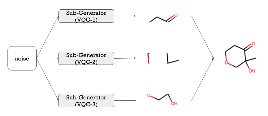
The sub-generator shares the same ansatz architecture as shown in Section II.3. Each ansatz circuit consists of the preparation of the initialization state, a single layer of a 4-qubit circuit, and the measurement. The initialization layer contains gates, and the rotation angles () are sampled from a uniform distribution. The parameterized layers (could be repeated for times) have CZ gates and one type of parameterized rotational gates, whose parameters () can be learned through back-propagation.
II.4 VQC of Quantum Discriminator
The quantum discriminator takes the molecular graph as input and classifies if this molecular graph is fake (from the generator) or real (from the data distribution). The VQC of the quantum discriminator consists of the amplitude encoding layer Schuld and Petruccione 2018 (), the strongly entangling layers () inspired by Schuld et al. 2020 and the measurement as shown in Section II.4. Amplitude encoding is used to encode the atom vector and bond matrix. The strongly entangling layers Schuld et al. 2020 have multiple CNOT gates and parameterized rotational gates as shown in Section II.4. In each layer, each qubit starts with parameterized rotational gates followed by a CNOT gate. The parameterized angles can be learned through back-propagation. The measurement takes the expectation value of one qubit, and this value is used to determine if the input molecular graph is real or fake. In our experiment, we use 9 qubits to encode the molecular graph and three-layer of strongly entanglement layers.
III Evaluation Metrics and Dataset
In this section, we will first introduce the evaluation method and metrics followed by the dataset we used to train the generative models.
III.1 Evaluation Method and Metrics
To evaluate the performance of different generative models, we first generate 5,000 noise samples from Gaussian distribution and variational quantum circuits for MolGAN and QuMolGAN, respectively. The generated noise samples are then fed into the trained generator of models to produce the atom vectors and bond matrices. In the end, these vectors and matrices are used to construct the molecular graphs. Seven evaluation metrics described below will be calculated from the molecular graphs.
Three quality metrics, i.e., validity, uniqueness, and novelty used in Samanta et al. 2018; Polykovskiy et al. 2020, and three drug properties, i.e., quantitative estimation of drug-likeness (QED), solubility, and synthesizability (SA), is used to compare different generative models in this work. Validity is the ratio of the valid molecules to all generated molecules, and uniqueness is the ratio of unique molecules to the valid molecules. Novelty is defined as the ratio of valid molecules which are not in the training dataset to all valid molecules. In addition, we also measure the diversity of generated molecules which is defined as how likely the generated molecules are to be diverse to the training dataset. We also report the valid and unique molecules (# molecules) from 5,000 noise samples. QED Bickerton et al. 2012 measures how likely a molecule is to be a drug based on the concept of desirability. Solubility reports the n-octanol-water partition coefficient (logP) Wildman and Crippen 1999 of the molecule that is the degree of a molecule being hydrophilic. SA Ertl and Schuffenhauer 2009 quantifies how easy a molecule is to be synthesized based on the molecular complexity and fragment contributions. These property metrics are calculated by using RDKit Landrum et al. 2022.
The Kullback–Leibler (KL) divergences Kullback and Leibler 1951 are also calculated, and it measures how well a probability distribution approximates another distribution. The probability distributions of a variety of physicochemical descriptors including BertzCT (molecular complexity index), MolLogP (Wildman-Crippen LogP value Wildman and Crippen 1999), MolWt (molecular weight), TPSA (molecular polar surface area), NumHAcceptors (number of hydrogen acceptors), NumHDonors (number of hydrogen donors), NumRotatableBonds (number of rotatable bonds), NumAliphaticRings (number of aliphatic rings), and NumAromaticRings (number of aromatic rings) for the generated molecules and the molecules of the training set are compared, and the corresponding KL-divergence scores are computed. Models able to capture the distributions of molecules in the training set will lead to small KL-divergence scores (). However, the final KL-divergence score () Brown et al. 2019 used in this paper is computed by
| (7) |
Therefore, the larger final KL-divergence score (S) means how well the model can capture these nine physicochemical distributions of molecules in the training set.
III.2 Dataset
All experiments of this work use the QM9 (Quantum Machines 9) Ramakrishnan et al. 2014 dataset. QM9 dataset is curated from the GDB-17 chemical database Ruddigkeit et al. 2012 which has approximately 166.4 billion molecules. QM9 consists of 133,171 molecules containing less than or equal to nine non-hydrogen atoms (carbon, nitrogen, oxygen, and fluorine). Figure 7 shows some molecules from the QM9 dataset, and Table 2 summarizes the drug properties of all molecules of the QM9 dataset.

| QM9 | |||
| # molecules | QED | Solubility | SA |
| 133,171 | 0.461 | 0.289 | 0.327 |
IV Computational Results and Discussion
In this section, we would like to computationally explore the potential benefits of our algorithms as compared to classical algorithms in small molecule discovery. We endeavored to find the best hyper-parameters for the base MolGAN. We first examined different complexities of generators (in Appendix A) and observed that MolGAN-HR (high reduction) has the best performance compared to other generator complexities. We then examined different input noise dimensions of generators (in Appendix B) and found out that the number of unique and valid molecules saturated at the input dimension equaling 4 (z_dim=4). In addition, we also tested different numbers of parameterized layers in the variational quantum circuit (VQC) (in Appendix C) and observed that MolGAN-HR with 3 parameterized layers of VQC as noise generator has the best performance compared to other numbers of parameterized layers. Therefore, in the following experiments, MolGAN-HR is used as the base model, and VQC with 3 parameterized layers is used as the base quantum circuit. In the first experiment, we substitute the noise generator of MolGAN with a VQC and discover the quantum advantage in the generated molecules with better drug properties. In the second experiment, we replace the generator of MolGAN with a VQC and show the potential of generating small molecules using a VQC. In the third experiment, we supplant the discriminator of MolGAN with a VQC and demonstrate the quantum advantage. All the combinations of the classical/quantum noise/generator/discriminator and their corresponding model name are shown in Table 1. All experiments are implemented by using Pennylane Bergholm et al. 2018 and PyTorch Paszke et al. 2017.
IV.1 Quantum Noise Generator
In the first experiment, we would like to compare the performance of QuMolGAN and classical MolGAN. We use the same hyper-parameters to train the QuMolGAN and classical MolGAN except for the learning rate. The learning rate of the quantum noise generator is 0.04, and the learning rate for the generator and discriminator is 0.001. The models are trained for 150 epochs. The WGAN (Wasserstein generative adversarial networks) loss Arjovsky et al. 2017 is used to train the models. QuMolGAN with three parameterized layers is used in this experiment. We have examined the input dimension of the generator at 2, 3, 4, and 8, and the results are shown in Table 3. It is noted that the QED, Solute, and SA scores in this table are calculated from the valid and unique molecules.
| z_dim=2 | z_dim=3 | z_dim=4 | z_dim=8 | ||||||||||||
| QuMolGAN | MolGAN | p-value | QuMolGAN | MolGAN | p-value | QuMolGAN | MolGAN | p-value | QuMolGAN | MolGAN | p-value | ||||
| # moleculesa | 363 | 657 | - | 414 | 2163 | - | 511 | 3085 | - | 646 | 3287 | - | |||
| QED | 0.489 | 0.475 | <0.01 | 0.489 | 0.465 | <0.01 | 0.473 | 0.465 | <0.05 | 0.474 | 0.470 | 0.149 | |||
| Solubility | 0.343 | 0.324 | <0.05 | 0.370 | 0.305 | <0.01 | 0.317 | 0.298 | <0.01 | 0.329 | 0.305 | <0.01 | |||
| SA | 0.367 | 0.336 | <0.05 | 0.310 | 0.307 | <0.05 | 0.308 | 0.296 | 0.246 | 0.309 | 0.307 | 0.581 | |||
| KL Score (S)b | 0.653 | 0.824 | - | 0.797 | 0.913 | - | 0.846 | 0.957 | - | 0.868 | 0.957 | - | |||
a Number of valid and unique molecules from 5,000 samples;
b From Equation 7;
The QuMolGAN is lacking in generating as many molecules as classical MolGAN which results in worse KL Scores. However, the QuMolGAN can generate molecules with significantly () better drug properties compared to the classical MolGAN particularly when the input noise dimension is small (z_dim=2 and z_dim=3). The drug properties distributions of MolGAN-generated and QuMolGAN-generated molecules are shown in Figure 8 for z_dim=2. It shows that QuMolGAN can generate molecules with better drug properties, particularly in QED. QuMolGAN has less probability to generate molecules whose QED is less than 0.4.


For the KL-divergence task, the MolLogP, BertzCT, and MolWt distributions of generated molecules are also shown in Figure 9 for z_dim=2. The classical MolGAN (blue) tends to generate molecules with similar distributions to the training set (grey) which results in a better KL-divergence score.

In the end, we randomly sample 32 valid and unique molecules from both MolGAN and QuMolGAN for z_dim=2, and the example molecules are shown in Figure 10. QuMolGAN can generate training-set-like molecules with better drug properties.


As mentioned in Brown et al. 2019, the goal-directed optimization of molecules tries to improve the demanded scores for the generated molecules. These scores reflect how well molecules satisfy the required properties. The goal is to find molecules that maximize the scoring function. In this experiment, we also would like to check if the quantum circuit can bring advantages to the MolGAN in the goal-directed benchmark. Therefore, we add a reward network into the original schema, and the updated schema is shown in Figure 11.

At this time, the generator is trained using a linear combination of the WGAN Arjovsky et al. 2017 loss and the RL Kaelbling et al. 1996 (reinforcement learning) loss:
| (8) |
where is a hyperparameter that controls the trade-off between WGAN loss and RL loss, and are the inputs to networks. Here, we set to weigh the loss between two components and the goal of improving SA, and QED to train MolGAN and QuMolGAN as suggested by the medical chemists. In addition, we also add the unique score into the goal to prevent the model from generating the same molecules. We have trained MolGAN and QuMolGAN with () and without () RL loss using the same hyperparameters for 150 epochs, and the results are shown in Table 4. The input noise dimension to the generator is 4 (z_dim =4). It is noted that the QED, Solute, and SA scores in this table are calculated from the valid molecules. In this table, the KL Scores of MolGAN are always greater than their quantum counterparts in different weights of RL loss. However, QuMolGAN can achieve a higher goal (from 0.47 to 0.57 in QED and from 0.29 to 0.76 in SA) compared to MolGAN (from 0.47 to 0.52 in QED and from 0.30 to 0.60 in SA) while . The solute is not the goal so these scores are close for MolGAN and QuMolGAN.
| MolGAN | QuMolGAN | |||||
| #of moleculesa | 2890 | 2700 | 696 | 534 | 309 | 116 |
| Validity | 80.40 | 78.48 | 68.76 | 70.02 | 70.32 | 42.94 |
| Uniqueness | 71.89 | 68.81 | 20.24 | 15.25 | 8.78 | 5.40 |
| QED | 0.47 | 0.48 | 0.52 | 0.47 | 0.49 | 0.57 |
| Solute | 0.31 | 0.31 | 0.45 | 0.32 | 0.30 | 0.44 |
| SA | 0.30 | 0.31 | 0.65 | 0.29 | 0.28 | 0.76 |
| KL Score (S)b | 0.95 | 0.94 | 0.58 | 0.92 | 0.82 | 0.31 |
a Number of valid and unique molecules from 5,000 samples;
b From Equation 7
IV.2 Quantum Generator
In the second experiment, we try to benchmark the advantage of the quantum circuit in the generator of GAN. We have tried to substitute the generator of MolGAN with a VQC described in Huang et al. 2021 for the small molecule generation. The performance of MolGAN with the quantum generator (MolGAN-QC) is reported in Table 5.
| # epoch | # moleculesa | validity | uniqueness | novelty | diversity | QED | Solubility | SA | KL Score (S)b |
| 1 | 73 | 79.39 | 4.49 | 100 | 1.00 | 0.43 | 0.75 | 0.24 | 0.24 |
| 2 | 54 | 76.37 | 3.45 | 100 | 1.00 | 0.47 | 0.75 | 0.24 | 0.25 |
| 3 | 43 | 78.47 | 2.68 | 100 | 1.00 | 0.48 | 0.75 | 0.11 | 0.28 |
| 4 | 29 | 78.61 | 1.80 | 100 | 1.00 | 0.48 | 0.75 | 0.13 | 0.29 |
| 5 | 30 | 77.93 | 1.88 | 100 | 1.00 | 0.48 | 0.75 | 0.14 | 0.30 |
| 6 | 40 | 78.37 | 2.49 | 100 | 1.00 | 0.48 | 0.75 | 0.09 | 0.21 |
| 7 | 29 | 80.27 | 1.76 | 100 | 1.00 | 0.47 | 0.75 | 0.06 | 0.28 |
| 8 | 39 | 78.91 | 2.41 | 100 | 1.00 | 0.48 | 0.75 | 0.16 | 0.28 |
| 9 | 41 | 74.66 | 2.68 | 100 | 1.00 | 0.48 | 0.75 | 0.22 | 0.25 |
| 10 | 29 | 79.74 | 1.78 | 100 | 1.00 | 0.48 | 0.75 | 0.08 | 0.27 |
a Number of valid and unique molecules from 2,048 samples from Gaussian distribution;
b From Equation 7;
Although the integration works smoothly, the training processing is time-consuming and resource-consuming. The average training time per step takes around 39 seconds in the Amazon EC2 C6a Metal Instance which results in approximately 3.5 days per epoch. In addition, the model has difficulty generating more valid and unique molecules after being trained for ten epochs. It fails to generate the training-data-like molecules even after ten epochs of training. Random-picked and cherry-picked examples of generated molecules are shown in Figure 12.

Most generated molecules are similar to the randomly sampled molecules in Figure 12. However, we demonstrate that the quantum generator has the potential to generate small molecules.
IV.3 Quantum Discriminator
In addition to substituting the generator architecture, the architecture with a quantum discriminator combined with the classical generator described in MolGAN has been experimented with. Our goal is to see if the quantum discriminator shows any advantage over its classical counterparts. We have found that the number of learnable parameters is significantly less than the classical ones while the model can still generate valid molecules. Furthermore, to conduct a fair comparison between the classical discriminator and the quantum one, we changed the MolGAN classical graph-based discriminator to the multiple-layer perceptron (MLP) architecture, which is more similar to our proposed quantum discriminator architecture, reduced the number of its training parameters, and found that quantum discriminator with 50 training parameters outperforms the classical discriminator with 22,500 parameters in terms of generated molecule properties and KL divergence. For simplicity, all the combinations of the classical/quantum noise/generator/discriminator are listed in Table 1. In this experiment, the noises of the generator are always sampled from the Gaussian distribution.
In the following subsections, we first present our proposed MolGAN-CQ and the training details. Second, we compare the results of MolGAN-CQ with MolGAN. In the end, we made architecture modifications from the Graph-Classical-Discriminator in MolGAN to the MLP-Classical-Discriminator (MolGAN-CC) and reduced the amount of the learnable parameters to make a fair comparison with MolGAN-CQ.
IV.3.1 MolGAN-CQ Architecture and Training Details
As illustrated in Figure 13, the model consists of two components: classical generator and quantum discriminator. To encode two generator outputs, a bond matrix, and an atom vector, into the quantum discriminator efficiently, we first flatten the bond matrix into a vector, which is subsequently concatenated with the atom vector to a new vector with the size of 450. After that, the resulting vector will be the input of the Q-Discriminator, composed of an amplitude embedding layer followed by 3 strongly entangling layers as described in Section II.4.

For the training details, at first, we followed the best hyper-parameters set in MolGAN. However, applying the same training details on MolGAN-CQ makes the training process hard to converge. Therefore, we change the learning rate from to for the generator to make it more stable. Moreover, we have experimented with the alternating training times between the classical generator and quantum discriminator with several sets, including (G, D)=(1, 5), (1, 8), (1, 10). We found out that training 1 step C-Generator followed by 10 steps Q-Discriminator stabilizes the training process. The other hyperparameters remain identical to the ones in MolGAN.
IV.3.2 Comparison with classical MolGAN
In this section, we compare MolGAN-CQ with MolGAN. We trained MolGAN according to the best hyper-parameter sets found in the previous section. Notice here, since training a quantum network is time-consuming, and the loss curve from classical MolGAN at epoch 30 shows the trend of convergence, both MolGAN-CQ and MolGAN were only trained to epoch 30 and evaluated at epoch 30 instead of epoch 150. After that, both models generate 5000 samples to do a further comparison. Table 6 demonstrates that MolGAN-CQ can generate valid and drug-like molecules. In addition, MolGAN-CQ can generate molecules with better drug properties, particularly in Solute and SA. However, compared to classical MolGAN, MolGAN-CQ does not have an advantage in KL divergence with training data probability. Figure 14 shows some molecules generated from MolGAN-CQ.
| MolGAN | MolGAN-CQ | |
| # of moleculesa | 2,693 | 730 |
| QED | 0.47 | 0.48 |
| Solute | 0.31 | 0.44 |
| SA | 0.31 | 0.66 |
| KL Score (S)b | 0.94 | 0.75 |
a Number of valid and unique molecules from 5,000 samples;
b From Equation 7

IV.3.3 Comparison with MolGAN-CC
In this section, MolGAN-CQ is compared with MolGAN-CC with different numbers of hidden layers to evaluate MolGAN-CQ’s capacity. To have a fair comparison, we modified the original graph-based network to a multiple-layer perceptron (MLP). Under this condition, the input of the MLP-based discriminator would be the same as the one in MolGAN-CQ’s quantum discriminator, a flattened vector instead of a graph. The network architecture of MolGAN-CC is shown in Figure 15.


Furthermore, since the discriminator of MolGAN-CQ only has 50 learnable parameters, we have tried to reduce the discriminator size of MolGAN-CC as small as possible for a fair and reasonable evaluation. However, the input vector is already a size of 450, it is not possible to decrease the parameter size to 50 in the classical MLP. Therefore, we have tried MolGAN-CC with 3 different parameter sizes of discriminator as shown in Table 7.
| # of layer in the MolGAN-CC discriminator | parameter size | |||
| MolGAN-CC-ERa |
|
22K | ||
| MolGAN-CC-HRb |
|
45K | ||
| MolGAN-CC-NRc |
|
82K |
a Extremely-reduction;
b Highly-reduction
c No-reduction;
Table 8 demonstrates that although MolGAN-CC-NR and MolGAN-CC-HR have a higher capacity to generate molecules whose molecule properties are more similar to the training data, MolGAN-CQ with only 50 parameters can achieve an outstanding performance compared to MolGAN-CC-ER with 22K parameters in terms of KL-score which shows the quantum advantage in the expression power. The distributions of molecular properties of MolLogP, MolWt, and BertzCT, generated from MolGAN-CC-ER, MolGAN-CQ, MolGAN, and QM9 are shown in Figure 16. As we can see from Figure 16, molecular properties from MolGAN are closer to the ones from the training data, QM9, compared to MolGAN-CQ and MolGAN-CC-ER. Nevertheless, MolGAN-CQ with only 50 parameters could generate molecules with similar distribution to the training data in comparison to MolGAN-CC-ER with 22K parameters.
| MolGAN-CQ | MolGAN-CC-ER | MolGAN-CC-HR | MolGAN-CC-NR | |
| # of parameters | 50 | 22K | 45K | 82K |
| #of moleculesa | 2,693 | 104 | 1919 | 2284 |
| QED | 0.47 | 0.51 | 0.49 | 0.5 |
| Solute | 0.44 | 0.63 | 0.35 | 0.38 |
| SA | 0.66 | 0.97 | 0.48 | 0.50 |
| KL Score (S)b | 0.75 | 0.28 | 0.84 | 0.81 |
a Number of valid and unique molecules from 5,000 samples;
b From Equation 7

V Conclusions
In this paper, we have explored the quantum advantage in small molecule drug discovery by substituting each part of MolGAN De Cao and Kipf 2018 with a VQC step by step and comparing its performance with the classical counterpart. In the first experiment, using a VQC as a noise generator to the classical GAN can generate small molecules with better drug properties including QED, SA, and LogP particularly when the input dimension to the generator is small, e.g., z_dim = 2 or z_dim = 3. However, QuMolGAN has difficulty generating as many unique molecules compared to classical MolGAN which results in a lower KL Score. In addition, this hybrid model achieves better performance in the goal-directed benchmark compared to the classical counterpart. In the second experiment, we substitute the classical generator with a VQC with the patch method Huang et al. 2021. We demonstrated the potential of generating training-set-like small molecules using a quantum generator. However, the training processing is resource-consuming and time-consuming even in the advanced classical computer. In the third experiment, we replace the classical discriminator with a VQC and compare its performance with the classical counterpart. This hybrid model MolGAN-CQ outperforms the classical counterpart in terms of generated molecule properties and the KL score. We also demonstrated that the hybrid model could generate valid molecules with only tens of learnable parameters in a quantum discriminator. The proposed hybrid model has the potential to be integrated into the Insilico Medicine Chemistry42TM Ivanenkov et al. 0 platform (Figure 17).
References
- Hingorani et al. (2019) A. D. Hingorani, V. Kuan, C. Finan, F. A. Kruger, A. Gaulton, S. Chopade, R. Sofat, R. J. MacAllister, J. P. Overington, H. Hemingway, et al., Scientific reports 9, 1 (2019).
- Abreu (2020) J. L. Abreu, Revista Daena (International Journal of Good Conscience) 15 (2020).
- Wouters et al. (2020) O. J. Wouters, M. McKee, and J. Luyten, Jama 323, 844 (2020).
- Aliper et al. (2016) A. Aliper, S. Plis, A. Artemov, A. Ulloa, P. Mamoshina, and A. Zhavoronkov, Molecular pharmaceutics 13, 2524 (2016).
- Kadurin et al. (2017a) A. Kadurin, A. Aliper, A. Kazennov, P. Mamoshina, Q. Vanhaelen, K. Khrabrov, and A. Zhavoronkov, Oncotarget 8, 10883 (2017a).
- Zhavoronkov (2018) A. Zhavoronkov, Artificial intelligence for drug discovery, biomarker development, and generation of novel chemistry (2018).
- Carracedo-Reboredo et al. (2021) P. Carracedo-Reboredo, J. Liñares-Blanco, N. Rodríguez-Fernández, F. Cedrón, F. J. Novoa, A. Carballal, V. Maojo, A. Pazos, and C. Fernandez-Lozano, Computational and Structural Biotechnology Journal 19, 4538 (2021).
- Kao et al. (2021) P.-Y. Kao, S.-M. Kao, N.-L. Huang, and Y.-C. Lin, in 2021 IEEE International Conference on Bioinformatics and Biomedicine (BIBM) (IEEE, 2021) pp. 2384–2391.
- Kolluri et al. (2022) S. Kolluri, J. Lin, R. Liu, Y. Zhang, and W. Zhang, The AAPS Journal 24, 1 (2022).
- Zhavoronkov et al. (2019) A. Zhavoronkov, Y. A. Ivanenkov, A. Aliper, M. S. Veselov, V. A. Aladinskiy, A. V. Aladinskaya, V. A. Terentiev, D. A. Polykovskiy, M. D. Kuznetsov, A. Asadulaev, et al., Nature biotechnology 37, 1038 (2019).
- Chan et al. (2019) H. S. Chan, H. Shan, T. Dahoun, H. Vogel, and S. Yuan, Trends in pharmacological sciences 40, 592 (2019).
- Schneider and Fechner (2005) G. Schneider and U. Fechner, Nature Reviews Drug Discovery 4, 649 (2005).
- Fischer et al. (2019) T. Fischer, S. Gazzola, and R. Riedl, Expert opinion on drug discovery 14, 791 (2019).
- Mouchlis et al. (2021) V. D. Mouchlis, A. Afantitis, A. Serra, M. Fratello, A. G. Papadiamantis, V. Aidinis, I. Lynch, D. Greco, and G. Melagraki, International journal of molecular sciences 22, 1676 (2021).
- Speck-Planche (2018) A. Speck-Planche, Future Medicinal Chemistry 10, 2021 (2018).
- Mamoshina et al. (2018) P. Mamoshina, L. Ojomoko, Y. Yanovich, A. Ostrovski, A. Botezatu, P. Prikhodko, E. Izumchenko, A. Aliper, K. Romantsov, A. Zhebrak, et al., Oncotarget 9, 5665 (2018).
- Zhavoronkov et al. (2020) A. Zhavoronkov, B. Zagribelnyy, A. Zhebrak, V. Aladinskiy, V. Terentiev, Q. Vanhaelen, D. S. Bezrukov, D. Polykovskiy, R. Shayakhmetov, A. Filimonov, et al., ChemRxiv (2020).
- Paul et al. (2021) D. Paul, G. Sanap, S. Shenoy, D. Kalyane, K. Kalia, and R. K. Tekade, Drug Discovery Today 26, 80 (2021).
- Martinelli (2022) D. Martinelli, Computers in Biology and Medicine , 105403 (2022).
- Goodfellow et al. (2014) I. Goodfellow, J. Pouget-Abadie, M. Mirza, B. Xu, D. Warde-Farley, S. Ozair, A. Courville, and Y. Bengio, Advances in neural information processing systems 27 (2014).
- Karras et al. (2017) T. Karras, T. Aila, S. Laine, and J. Lehtinen, arXiv preprint arXiv:1710.10196 (2017).
- Isola et al. (2017) P. Isola, J.-Y. Zhu, T. Zhou, and A. A. Efros, in Proceedings of the IEEE conference on computer vision and pattern recognition (2017) pp. 1125–1134.
- Zhu et al. (2017) J.-Y. Zhu, T. Park, P. Isola, and A. A. Efros, in Proceedings of the IEEE international conference on computer vision (2017) pp. 2223–2232.
- Karras et al. (2019) T. Karras, S. Laine, and T. Aila, in Proceedings of the IEEE/CVF conference on computer vision and pattern recognition (2019) pp. 4401–4410.
- Jangid et al. (2022) D. K. Jangid, N. R. Brodnik, A. Khan, M. G. Goebel, M. P. Echlin, T. M. Pollock, S. H. Daly, and B. Manjunath, Integrating Materials and Manufacturing Innovation , 1 (2022).
- Kadurin et al. (2017b) A. Kadurin, S. Nikolenko, K. Khrabrov, A. Aliper, and A. Zhavoronkov, Molecular pharmaceutics 14, 3098 (2017b).
- Vanhaelen et al. (2020) Q. Vanhaelen, Y.-C. Lin, and A. Zhavoronkov, ACS Medicinal Chemistry Letters 11, 1496 (2020).
- Xu et al. (2021) M. Xu, J. Cheng, Y. Liu, and W. Huang, in 2021 IEEE Symposium on Computers and Communications (ISCC) (IEEE, 2021) pp. 1–6.
- Guimaraes et al. (2017) G. L. Guimaraes, B. Sanchez-Lengeling, C. Outeiral, P. L. C. Farias, and A. Aspuru-Guzik, arXiv preprint arXiv:1705.10843 (2017).
- Yu et al. (2017) L. Yu, W. Zhang, J. Wang, and Y. Yu, in Proceedings of the Thirty-First AAAI Conference on Artificial Intelligence (2017) pp. 2852–2858.
- Prykhodko et al. (2019) O. Prykhodko, S. V. Johansson, P.-C. Kotsias, J. Arús-Pous, E. J. Bjerrum, O. Engkvist, and H. Chen, Journal of Cheminformatics 11, 1 (2019).
- Kotsias et al. (2020) P.-C. Kotsias, J. Arús-Pous, H. Chen, O. Engkvist, C. Tyrchan, and E. J. Bjerrum, Nature Machine Intelligence 2, 254 (2020).
- De Cao and Kipf (2018) N. De Cao and T. Kipf, arXiv preprint arXiv:1805.11973 (2018).
- Jayatunga et al. (2022) M. K. Jayatunga, W. Xie, L. Ruder, U. Schulze, and C. Meier, Nature reviews. Drug Discovery (2022).
- Neukart et al. (2017) F. Neukart, G. Compostella, C. Seidel, D. Von Dollen, S. Yarkoni, and B. Parney, Frontiers in ICT 4, 29 (2017).
- Harwood et al. (2021) S. Harwood, C. Gambella, D. Trenev, A. Simonetto, D. Bernal, and D. Greenberg, IEEE Transactions on Quantum Engineering 2, 1 (2021).
- Orus et al. (2019) R. Orus, S. Mugel, and E. Lizaso, Reviews in Physics 4, 100028 (2019).
- Liu and Ma (2022) G. Liu and W. Ma, Information Sciences 598, 75 (2022).
- Du et al. (2022) Y. Du, Y. Yang, D. Tao, and M.-H. Hsieh, arXiv preprint arXiv:2301.01597 (2022).
- Yin et al. (2022) X.-F. Yin, Y. Du, Y.-Y. Fei, R. Zhang, L.-Z. Liu, Y. Mao, T. Liu, M.-H. Hsieh, L. Li, N.-L. Liu, D. Tao, Y.-A. Chen, and J.-W. Pan, Phys. Rev. Lett. 128, 110501 (2022).
- Rudolph et al. (2022) M. S. Rudolph, N. B. Toussaint, A. Katabarwa, S. Johri, B. Peropadre, and A. Perdomo-Ortiz, Physical Review X 12, 031010 (2022).
- Aspuru-Guzik et al. (2005) A. Aspuru-Guzik, A. D. Dutoi, P. J. Love, and M. Head-Gordon, Science 309, 1704 (2005).
- Lanyon et al. (2010) B. P. Lanyon, J. D. Whitfield, G. G. Gillett, M. E. Goggin, M. P. Almeida, I. Kassal, J. D. Biamonte, M. Mohseni, B. J. Powell, M. Barbieri, et al., Nature chemistry 2, 106 (2010).
- Peruzzo et al. (2014) A. Peruzzo, J. McClean, P. Shadbolt, M.-H. Yung, X.-Q. Zhou, P. J. Love, A. Aspuru-Guzik, and J. L. O’brien, Nature communications 5, 1 (2014).
- O’Malley et al. (2016) P. J. O’Malley, R. Babbush, I. D. Kivlichan, J. Romero, J. R. McClean, R. Barends, J. Kelly, P. Roushan, A. Tranter, N. Ding, et al., Physical Review X 6, 031007 (2016).
- Kandala et al. (2017) A. Kandala, A. Mezzacapo, K. Temme, M. Takita, M. Brink, J. M. Chow, and J. M. Gambetta, Nature 549, 242 (2017).
- Cao et al. (2019) Y. Cao, J. Romero, J. P. Olson, M. Degroote, P. D. Johnson, M. Kieferová, I. D. Kivlichan, T. Menke, B. Peropadre, N. P. D. Sawaya, S. Sim, L. Veis, and A. Aspuru-Guzik, Chemical Reviews 119, 10856 (2019), pMID: 31469277, https://doi.org/10.1021/acs.chemrev.8b00803 .
- Quantum et al. (2020) G. A. Quantum, Collaborators*†, F. Arute, K. Arya, R. Babbush, D. Bacon, J. C. Bardin, R. Barends, S. Boixo, M. Broughton, B. B. Buckley, et al., Science 369, 1084 (2020).
- Gao et al. (2021a) Q. Gao, H. Nakamura, T. P. Gujarati, G. O. Jones, J. E. Rice, S. P. Wood, M. Pistoia, J. M. Garcia, and N. Yamamoto, The Journal of Physical Chemistry A 125, 1827 (2021a).
- Shee et al. (2022) Y. Shee, T.-L. Yeh, J.-Y. Hsiao, A. Yang, Y.-C. Lin, and M.-H. Hsieh, arXiv preprint arXiv:2210.02977 (2022).
- Cao et al. (2018) Y. Cao, J. Romero, and A. Aspuru-Guzik, IBM Journal of Research and Development 62, 6 (2018).
- Li et al. (2021) J. Li, R. O. Topaloglu, and S. Ghosh, IEEE Transactions on Quantum Engineering 2, 1 (2021).
- Feynman et al. (1982) R. P. Feynman et al., Int. j. Theor. phys 21 (1982).
- Grover (1996) L. K. Grover, in Proceedings of the twenty-eighth annual ACM symposium on Theory of computing (1996) pp. 212–219.
- Coppersmith (2002) D. Coppersmith, arXiv preprint quant-ph/0201067 (2002).
- Shor (1994) P. W. Shor, in Proceedings 35th annual symposium on foundations of computer science (Ieee, 1994) pp. 124–134.
- Kitaev (1995) A. Y. Kitaev, arXiv preprint quant-ph/9511026 (1995).
- Giovannetti et al. (2004) V. Giovannetti, S. Lloyd, and L. Maccone, Science 306, 1330 (2004).
- Giovannetti et al. (2006) V. Giovannetti, S. Lloyd, and L. Maccone, Physical review letters 96, 010401 (2006).
- Lloyd (2008) S. Lloyd, Science 321, 1463 (2008).
- Komar et al. (2014) P. Komar, E. M. Kessler, M. Bishof, L. Jiang, A. S. Sørensen, J. Ye, and M. D. Lukin, Nature Physics 10, 582 (2014).
- Chao and Reichardt (2018) R. Chao and B. W. Reichardt, npj Quantum Information 4, 1 (2018).
- Bharti et al. (2022) K. Bharti, A. Cervera-Lierta, T. H. Kyaw, T. Haug, S. Alperin-Lea, A. Anand, M. Degroote, H. Heimonen, J. S. Kottmann, T. Menke, et al., Reviews of Modern Physics 94, 015004 (2022).
- Arute et al. (2019) F. Arute, K. Arya, R. Babbush, D. Bacon, J. C. Bardin, R. Barends, R. Biswas, S. Boixo, F. G. Brandao, D. A. Buell, et al., Nature 574, 505 (2019).
- Zhong et al. (2020) H.-S. Zhong, H. Wang, Y.-H. Deng, M.-C. Chen, L.-C. Peng, Y.-H. Luo, J. Qin, D. Wu, X. Ding, Y. Hu, et al., Science 370, 1460 (2020).
- Quesada et al. (2018) N. Quesada, J. M. Arrazola, and N. Killoran, Physical Review A 98, 062322 (2018).
- Gao et al. (2021b) X. Gao, E. R. Anschuetz, S.-T. Wang, J. I. Cirac, and M. D. Lukin, arXiv preprint arXiv:2101.08354 (2021b).
- Chen et al. (2020) S. Y.-C. Chen, C.-H. H. Yang, J. Qi, P.-Y. Chen, X. Ma, and H.-S. Goan, IEEE Access 8, 141007 (2020).
- Du et al. (2020) Y. Du, M.-H. Hsieh, T. Liu, and D. Tao, Physical Review Research 2, 033125 (2020).
- Du et al. (2021a) Y. Du, M.-H. Hsieh, T. Liu, S. You, and D. Tao, PRX Quantum 2, 040337 (2021a).
- Du et al. (2021b) Y. Du, M.-H. Hsieh, T. Liu, D. Tao, and N. Liu, Physical Review Research 3, 023153 (2021b).
- Blunt et al. (2022) N. S. Blunt, J. Camps, O. Crawford, R. Izsák, S. Leontica, A. Mirani, A. E. Moylett, S. A. Scivier, C. Sünderhauf, P. Schopf, et al., arXiv preprint arXiv:2206.00551 (2022).
- Gircha et al. (2021) A. Gircha, A. S. Boev, K. Avchaciov, P. Fedichev, and A. K. Fedorov, arXiv preprint arXiv:2108.11644 (2021).
- Lloyd and Weedbrook (2018) S. Lloyd and C. Weedbrook, Physical review letters 121, 040502 (2018).
- Huang et al. (2021) H.-L. Huang, Y. Du, M. Gong, Y. Zhao, Y. Wu, C. Wang, S. Li, F. Liang, J. Lin, Y. Xu, et al., Physical Review Applied 16, 024051 (2021).
- Dallaire-Demers and Killoran (2018) P.-L. Dallaire-Demers and N. Killoran, Physical Review A 98, 012324 (2018).
- Romero and Aspuru-Guzik (2021) J. Romero and A. Aspuru-Guzik, Advanced Quantum Technologies 4, 2000003 (2021).
- Ivanenkov et al. (0) Y. A. Ivanenkov, D. Polykovskiy, D. Bezrukov, B. Zagribelnyy, V. Aladinskiy, P. Kamya, A. Aliper, F. Ren, and A. Zhavoronkov, Journal of Chemical Information and Modeling 0, null (0), pMID: 36728505, https://doi.org/10.1021/acs.jcim.2c01191 .
- Bergholm et al. (2018) V. Bergholm, J. Izaac, M. Schuld, C. Gogolin, M. S. Alam, S. Ahmed, J. M. Arrazola, C. Blank, A. Delgado, S. Jahangiri, et al., arXiv preprint arXiv:1811.04968 (2018).
- Paszke et al. (2017) A. Paszke, S. Gross, S. Chintala, G. Chanan, E. Yang, Z. DeVito, Z. Lin, A. Desmaison, L. Antiga, and A. Lerer, NIPS 2017 Autodiff Workshop (2017).
- Schuld and Petruccione (2018) M. Schuld and F. Petruccione, Supervised learning with quantum computers, Vol. 17 (Springer, 2018).
- Schuld et al. (2020) M. Schuld, A. Bocharov, K. M. Svore, and N. Wiebe, Physical Review A 101, 032308 (2020).
- Samanta et al. (2018) B. Samanta, A. De, N. Ganguly, and M. Gomez-Rodriguez, arXiv preprint arXiv:1802.05283 (2018).
- Polykovskiy et al. (2020) D. Polykovskiy, A. Zhebrak, B. Sanchez-Lengeling, S. Golovanov, O. Tatanov, S. Belyaev, R. Kurbanov, A. Artamonov, V. Aladinskiy, M. Veselov, et al., Frontiers in pharmacology 11, 565644 (2020).
- Bickerton et al. (2012) G. R. Bickerton, G. V. Paolini, J. Besnard, S. Muresan, and A. L. Hopkins, Nature chemistry 4, 90 (2012).
- Wildman and Crippen (1999) S. A. Wildman and G. M. Crippen, Journal of chemical information and computer sciences 39, 868 (1999).
- Ertl and Schuffenhauer (2009) P. Ertl and A. Schuffenhauer, Journal of cheminformatics 1, 1 (2009).
- Landrum et al. (2022) G. Landrum, P. Tosco, B. Kelley, Ric, sriniker, gedeck, R. Vianello, NadineSchneider, E. Kawashima, A. Dalke, D. N, D. Cosgrove, B. Cole, M. Swain, S. Turk, AlexanderSavelyev, G. Jones, A. Vaucher, M. Wójcikowski, I. Take, D. Probst, K. Ujihara, V. F. Scalfani, guillaume godin, A. Pahl, F. Berenger, JLVarjo, strets123, JP, and DoliathGavid, rdkit/rdkit: 2022_03_1 (q1 2022) release (2022).
- Kullback and Leibler (1951) S. Kullback and R. A. Leibler, The annals of mathematical statistics 22, 79 (1951).
- Brown et al. (2019) N. Brown, M. Fiscato, M. H. Segler, and A. C. Vaucher, Journal of chemical information and modeling 59, 1096 (2019).
- Ramakrishnan et al. (2014) R. Ramakrishnan, P. O. Dral, M. Rupp, and O. A. Von Lilienfeld, Scientific data 1, 1 (2014).
- Ruddigkeit et al. (2012) L. Ruddigkeit, R. Van Deursen, L. C. Blum, and J.-L. Reymond, Journal of chemical information and modeling 52, 2864 (2012).
- Arjovsky et al. (2017) M. Arjovsky, S. Chintala, and L. Bottou, in International conference on machine learning (PMLR, 2017) pp. 214–223.
- Kaelbling et al. (1996) L. P. Kaelbling, M. L. Littman, and A. W. Moore, Journal of artificial intelligence research 4, 237 (1996).
- Srivastava et al. (2014) N. Srivastava, G. Hinton, A. Krizhevsky, I. Sutskever, and R. Salakhutdinov, The journal of machine learning research 15, 1929 (2014).
- Padala et al. (2021) M. Padala, D. Das, and S. Gujar, in International Conference on Neural Information Processing (Springer, 2021) pp. 558–569.
- LeCun et al. (1998) Y. LeCun, L. Bottou, Y. Bengio, and P. Haffner, Proceedings of the IEEE 86, 2278 (1998).
- Liu et al. (2015) Z. Liu, P. Luo, X. Wang, and X. Tang, in Proceedings of the IEEE international conference on computer vision (2015) pp. 3730–3738.
- Benedetti et al. (2019) M. Benedetti, E. Lloyd, S. Sack, and M. Fiorentini, Quantum Science and Technology 4, 043001 (2019).
- Sim et al. (2019) S. Sim, P. D. Johnson, and A. Aspuru-Guzik, Advanced Quantum Technologies 2, 1900070 (2019).
- McClean et al. (2018) J. R. McClean, S. Boixo, V. N. Smelyanskiy, R. Babbush, and H. Neven, Nature communications 9, 1 (2018).
- Zhang et al. (2021) K. Zhang, M.-H. Hsieh, L. Liu, and D. Tao, arXiv preprint arXiv:2112.15002 (2021).
- Zhang et al. (2022) K. Zhang, L. Liu, M.-H. Hsieh, and D. Tao, in Advances in Neural Information Processing Systems (2022).
Appendix A Different Generator Complexities
We would like to explore the relationship between the generator complexity and the training data. The generator of MolGAN consists of multiple dense layers (linear layer followed by activation layer and dropout layer Srivastava et al. 2014). We train three models with different generator complexities. The generator of the first model has the same amount of parameters as the original MolGAN De Cao and Kipf 2018. The generator of the second model only has approximately 15% of the parameters as the original MolGAN, and we call this model MolGAN-HR (high reduction). The generator of the third model merely has approximately 2% of the parameters as the original MolGAN, and we call this model MolGAN-ER (extreme reduction). These three models are trained using the same hyperparameters. The batch size is 128. The models are trained for 150 epochs. The learning rate is 0.001 for both the generator and discriminator. The discriminator is updated three times followed by updating the generator once. We evaluate each model using the generator from 150 epochs, and the results are shown in Table 9. In this table, MolGAN-HR can generate the most valid and unique molecules which results in the highest KL Score. The QED, Solute, and SA scores in this table are calculated from the valid molecules.
| Model | # moleculesd | validity | uniqueness | novelty | diversity | QED | Solubility | SA | KL Score (S)e |
| MolGANa | 995 | 78.54 | 25.34 | 59.56 | 0.57 | 0.47 | 0.31 | 0.28 | 0.893 |
| MolGAN-HRb | 3191 | 78.34 | 81.47 | 64.33 | 0.59 | 0.47 | 0.31 | 0.29 | 0.954 |
| MolGAN-ERc | 2826 | 75.84 | 74.53 | 67.14 | 0.67 | 0.47 | 0.31 | 0.32 | 0.945 |
a 396,610 parameters;
b Highly-reduction (59,202 parameters);
c Extremely-reduction (7,794 parameters);
d Number of valid and unique molecules from 5,000 samples;
e From Equation 7;
Appendix B Varying the Input Noise Dimension of Generator
Padala et al Padala et al. 2021 have examined the effect of input noise dimension in GANs in generating the Gaussian distribution, the handwritten digit recognition LeCun et al. 1998, and the celebrity image classification Liu et al. 2015. They observed a significant effect on the results when the input noise dimension is alternated. They also claimed that the optimal noise dimension is depended on the dataset and loss function used. Inspired by their work, we would like to examine the optimal input noise dimension for the task of small molecular generation using the QM9 dataset for MolGAN and QuMolGAN. The input noise dimension is varied from 1 to 8 for the MolGAN-HR, and the results are shown in Table 10. For QuMolGAN-HR, we only examine the ansatz with 2, 3, 4, and 8 qubits, and the experimental results are shown in Table 11. These models are trained for 150 epochs. The learning rates of the discriminator and generator are 0.001, and the learning rate of the quantum circuit is 0.04. The QED, Solute, and SA scores in this table are calculated from the valid molecules. From these two tables, the number of valid and unique molecules saturates when the input dimension (z_dim) goes beyond 4. The KL Score of MolGAN-HR oscillates between 0.94 and 0.96, and the KL Score of QuMolGAN-HR has the best KL Score as z_dim=4.
| z-dim | # moleculesa | validity | uniqueness | novelty | diversity | QED | Solubility | SA | KL Score (S)b |
| 8 | 3204 | 80.04 | 80.06 | 64.67 | 0.62 | 0.47 | 0.31 | 0.30 | 0.946 |
| 7 | 3206 | 80.42 | 79.73 | 65.61 | 0.74 | 0.47 | 0.30 | 0.30 | 0.957 |
| 6 | 2898 | 77.76 | 74.54 | 61.34 | 0.72 | 0.47 | 0.30 | 0.29 | 0.937 |
| 5 | 3104 | 78.86 | 78.72 | 63.78 | 0.62 | 0.47 | 0.30 | 0.30 | 0.955 |
| 4 | 2930 | 81.26 | 72.11 | 63.82 | 0.65 | 0.47 | 0.30 | 0.30 | 0.941 |
| 3 | 1850 | 75.36 | 49.10 | 66.43 | 0.68 | 0.47 | 0.31 | 0.30 | 0.926 |
| 2 | 571 | 73.56 | 15.52 | 72.92 | 0.66 | 0.48 | 0.32 | 0.34 | 0.868 |
| 1 | 33 | 59.16 | 1.12 | 77.45 | 0.72 | 0.47 | 0.33 | 0.29 | 0.687 |
a Number of valid and unique molecules from 5,000 samples;
b From Equation 7;
| # qubitsa | # moleculesb | validity | uniqueness | novelty | diversity | QED | Solubility | SA | KL Score (S)c |
| 8 | 515 | 73.94 | 13.93 | 60.05 | 0.62 | 0.46 | 0.31 | 0.27 | 0.785 |
| 4 | 534 | 70.02 | 15.25 | 71.04 | 0.70 | 0.47 | 0.32 | 0.29 | 0.894 |
| 3 | 301 | 64.74 | 9.30 | 66.23 | 0.58 | 0.50 | 0.34 | 0.38 | 0.782 |
| 2 | 194 | 63.68 | 6.09 | 66.02 | 0.69 | 0.49 | 0.36 | 0.45 | 0.570 |
a Number of qubits of quantum circuit;
b Number of valid and unique molecules from 5,000 samples;
c From Equation 7;
Appendix C Number of Parameterized Layers of Variational Quantum Circuit
Variational quantum circuits (VQCs) can be considered machine learning models with remarkable expressive power for a variety of data-driven tasks, such as supervised learning and generative modeling Benedetti et al. 2019. VQCs consists of three ingredients: a fixed initial state, e.g., the zero state, a quantum circuit, parameterized by a set of learnable parameters, and the measurement as shown in Section II.2. A quantum circuit is composed of an initialization layer and parameterized layer(s). The initialization layer brings randomness to the VQC, and the parameters of parameterized layer(s) can be learned through back-propagation. One challenge in implementing variational quantum algorithms is to choose an effective circuit that well represents the solution space while maintaining a low circuit depth and the number of parameters Sim et al. 2019. Increasing the number of parameterized layers of VQC has the potential to improve the impressive power of VQC and its performance. However, it may face the problem of Barren plateaus McClean et al. 2018; Zhang et al. 2021; Zhang et al. 2022 and longer computational time. In this experiment, we would like to find the optimal number of parameterized layers that can generate the most unique and valid molecules for QuMolGAN-HR. We have examined one to five parameterized layers, and the results are shown in Table 12. In this table, QuMolGAN-HR achieves the best KL Score when the VQC has three parameterized layers.
| # layersa | # moleculesb | validity | uniqueness | novelty | diversity | QED | Solubility | SA | KL Score (S)c |
| 5 | 375 | 70.10 | 10.70 | 70.44 | 0.63 | 0.47 | 0.32 | 0.31 | 0.738 |
| 4 | 377 | 52.04 | 14.49 | 64.64 | 0.57 | 0.46 | 0.32 | 0.27 | 0.701 |
| 3 | 443 | 72.40 | 12.24 | 69.20 | 0.68 | 0.50 | 0.36 | 0.32 | 0.784 |
| 2 | 435 | 76.06 | 11.44 | 71.00 | 0.61 | 0.45 | 0.33 | 0.28 | 0.765 |
| 1 | 165 | 75.98 | 4.34 | 67.81 | 0.66 | 0.44 | 0.32 | 0.26 | 0.702 |
a Number of parameterized layers;
b Number of valid and unique molecules from 5,000 samples;
c From Equation 7;
Appendix D Chemistry42TM
