UTF8mc
MPC Builder for Autonomous Drive:
Automatic Generation of MPCs for Motion Planning and Control
Thanks: This work was supported by J-QuAD DYNAMICS Inc., Tokyo, Japan. This work was also supported by a research grant (C) from Tateisi Science and Technology Foundation.
Abstract
This study presents a new framework for vehicle motion planning and control based on the automatic generation of model predictive controllers (MPCs) named MPC Builder. In this framework, several components necessary for MPC, such as prediction models, constraints, and cost functions, are prepared in advance. The MPC Builder then generates various MPCs online in a unified manner according to traffic situations. This scheme enabled us to represent various driving tasks with less design effort than typical switched MPC systems. The proposed framework was implemented considering the continuation/generalized minimum residual (C/GMRES) method optimization solver, which can reduce computational costs. Finally, numerical experiments on multiple driving scenarios were presented.
Index Terms:
Motion Planning and Control, Autonomous Driving, Multi-task Planning, Model Predictive ControlI INTRODUCTION
Autonomous driving (AD) is expected to reduce traffic accidents and improve transportation comfort. Motion planning is an essential component for realizing AD. The motion planner controls the ego vehicle to accomplish various driving tasks, such as following the leading vehicle, changing lanes, overtaking, and pausing, while considering traffic rules, passenger comfort, and safety.
Model predictive control (MPC) [1] is a promising vehicle motion planning and control technique. As MPC is a finite-time optimal control based on a receding horizon scheme, flexible motion planning and control can be achieved by incorporating various control requirements into cost functions and constraints. MPC performs well particularly in dynamic environments by embedding the prediction models of surrounding road users into the constraints of the optimization problem [2]. Consequently, MPC has been applied to complex driving scenarios in the presence of other road users, such as lane changing [3, 4, 5], obstacle avoidance [6, 7], pedestrian avoidance [8, 9], adaptive cruise control (ACC) [10], and turning and crossing at intersections [11, 12].

However, to apply MPC to an actual traffic environment, addressing various driving tasks and preparing many MPCs in the design stage are required. This requires intensive design efforts for the AD designers. Thus, developing a unified scheme for MPCs that can deal with diverse environments and multiple driving tasks is recommended. Previous studies have proposed switched MPC systems that switch multiple MPCs designed for specific driving tasks [13, 14, 15, 16]. While these methods are capable of handling various driving tasks, the number of scenarios they can address is limited due to the insufficient number of MPCs available to cover all possible driving situations.
Based on this information, this study presents a new framework for the automatic generation of MPCs, called MPC Builder, which online designs MPCs for various driving tasks according to traffic situations. The proposed framework first decomposes the general formulations of MPC into reusable primitives as representations of subtasks. The primitives are defined as a set of state spaces, prediction models, cost functions, and constraints to achieve a control requirement. The proposed framework then combines the primitives using a binary operator for the primitives to generate optimization problems in real-time, as shown in Fig. 1. This scheme can represent diverse driving tasks sequentially and in parallel with fewer design elements than the switched MPC system, because the primitives can be replaced and add-on as common components of multiple MPCs.
The generated MPCs can vary the state space and the prediction models depending on the other road users considered. In order to work in real-time, even in high-dimensional state spaces, we implemented the proposed system considering the continuation/generalized minimum residual (C/GMRES) method [17], which is a fast nonlinear MPC solver based on the continuity of the optimal solution. Through numerical simulations, four typical driving scenarios were targeted, and the driving behaviors and real-time performance of the proposed method were demonstrated.
II RELATED WORK
AD requires diversified driving tasks to adapt to complex traffic environments. Many studies on AD have addressed single tasks, such as highway cruising and obstacle avoidance. Previous studies have addressed multi-task vehicle motion planning in MPC frameworks. Kim et al. applied an adaptive potential field to represent various driving behaviors [18]. Liu et al. proposed a nonlinear MPC that performs multiple driving tasks by convexly relaxing the mixed-integer problem [19]. Although this MPC can implicitly represent various driving tasks as a convex relaxation of the mixed-integer problem, realizing more driving tasks in a single MPC remains challenging. Some studies have proposed switched MPC systems that switch MPCs according to the driving situation [13, 14, 15, 16]. These methods switch weight parameters [5, 13], reference speed and lane [14], safety constraints [15], and cost functions and constraints [16] to accomplish various driving tasks depending on the traffic situation. Although these MPCs are designed for different driving tasks, they share common elements. As a result, the switched MPC system is redundant for various driving tasks. The proposed framework reduces the redundancy and implementation effort by representing multiple MPCs by combining common primitives. The proposed framework is also a general concept of switched MPC system that switches not only the parameters of the cost function and constraints but also the state space and the prediction model.
The proposed framework represents various MPCs for various driving tasks in a unified manner. It is inspired by the Riemannian Motion Policies (RMP) [20], which combines primitive motion policies for generating a single motion. Some studies have applied RMP to AD [21]. As RMP is based on stationary dynamics, it cannot manage the transient dynamics of the control target, whereas our proposed method can consider any dynamic model by combining the elements of MPC.
III MPC BUILDER
III-A Concept of MPC Builder
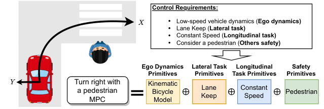
We propose the MPC Builder, which provides a unified framework for generating MPCs for various AD tasks. The concept of the MPC Builder is to compose MPCs to achieve various tasks from a set of primitives that express the common elements of the target tasks. The primitives are small control requirements that are defined in advance. The requirements include the following.
- •
Predictive models for the AD vehicle and/or other agents
- •
Safety constraints for other agents and/or obstacles
- •
To achieve a part of the driving objective (subtask)
For example, in a right turn with a pedestrian, as shown in Fig. 2, the requirements are to maintain the lane and speed while considering low-speed vehicle dynamics and pedestrian safety. In the proposed framework, these control requirements are defined in small MPC components called MPC primitive, which are combined to represent driving tasks. Some of these control requirements are not only available for right-turning, but also for other driving tasks. Therefore, we decompose some MPC for specific driving tasks into MPC primitives and combine them to represent various driving tasks.
III-B System Overview
Based on the aforementioned ideas, we propose a system that performs various driving tasks by building MPCs according to the traffic situation. Figure 3 shows the proposed system outline. The MPC Builder realizes the desired tasks by receiving reference path information from the route planner and observation from the recognition module with localization and detection. The task command is a symbolic command with parameters to realize the desired behavior (e.g., changing lanes, stopping 100m ahead, etc). The MPC Builder constructs the optimization problem online to be solved in the MPC framework using this information. Finally, the MPC solver solves this optimization problem to calculate and output the control inputs and predictive states in each control cycle.
The MPC Builder consists of three modules: MPC Primitive Pool, Aggregator, and MPC Composer. MPC Primitive Pool stores the MPC primitives defined later (section III-C). Aggregator selects and makes a set of the required MPC primitives according to the driving task command and observation (section IV-B2). MPC Composer formulates the optimization problem at the control cycle by composing all elements of a set of MPC primitive (section III-D).
III-C Definition of MPC primitive
Here, we define the MPC primitive, which is the core idea of the proposed method.
III-C1 General formulation of MPC
This section reviews the general formulation of the optimization problem before defining MPC primitives. MPC finds a series of optimal control inputs by solving the optimization problem with the finite-time future prediction of every control cycle. We can obtain the state prediction and optimal control input by solving the following optimization problem at time :
| (1) | ||||
| (2) | ||||
| (3) | ||||
| (4) | ||||
| (5) | ||||
| (6) |
where is the observed value of the state vector at time ; denotes the predicted values and and are the predicted state and control input vectors for the -th step future at time . and denote the state and control spaces, respectively. and are the length and time intervals of the prediction horizon, respectively. is a cost function that is minimized. is a state-prediction function with Euler discretization that represents the dynamics of the control target. and are function vectors of the inequality and equality constraints, respectively. The notation denotes that the function is applied to the entire prediction horizon from to . and are the sizes of the inequality and equality constraints, respectively. The prediction horizon length and control horizon length are the same, in this study.
III-C2 Definition of MPC primitive
The proposed framework decomposes the optimization problems represented by Eq. (7) into small components, called MPC primitives, and assembles the optimization problem . With MPC primitives as design elements, we assume that they are designed manually from the control requirements of multiple driving tasks as described in section III-A. In Eq. (7), the smallest primitives of the optimization problem are , and . However, these smallest primitives alone are not sufficient to represent the control requirements. For example, a cost function and constraints are required to express the constant speed control requirement, as shown in Fig. 2. Thus, we define the MPC primitive as a tuple to represent the control requirements:
| (8) |
where each element can be an empty set, different from Eq. (7). is also assumed to be common for all aimed tasks and MPC primitives because the control target vehicle is identical.
III-D Composition of MPC primitives
MPC Composer shown in the Fig. 3 composes the optimization problem from a set of MPC primitives . First, we assume that all MPC primitives are formulated with a common prediction horizon; horizon length and time interval are common. Under this assumption, the following additive binary operator is defined between the two MPC primitives:
| (9) |
where is the binary operator combining two MPC primitives defined in Algorithm 1. In the Algorithm 1, the state space is extended in line 5. The Cartesian product of the state spaces denotes the variable space concatenation. In lines 8 to 14, the state prediction function, cost function, and the constraints are extended in the extended state space: , , , and . Note that the product with a null vector of is defined as for vector . Using this operator iteratively, the MPC Composer shown in Fig. 3 composes the optimization problem from a MPC primitive set at every control cycle:
| (10) |
III-E Example of MPC Composition
This section illustrates an example of the composition of MPC primitives using the turn-right scenario with a pedestrian, as shown in Fig. 2 introduced in section III-A. We prepared the following four primitives: kinematic bicycle model (KBM) [22], lane keep, constant speed, and pedestrian primitives to represent this driving scenario. Table I lists the detailed formulations of the MPC primitives. MPC Composer composes these primitives and obtains the following optimization problem:
| (11) | ||||
| (12) | ||||
| (13) | ||||
| (14) | ||||
| (15) | ||||
| (16) |
where and are the state spaces of ego vehicles and pedestrians, respectively. The control input space are the time derivatives of the steering angle and acceleration of the ego vehicle, respectively. , and are the elements of the kinematic bicycle model, lane keep, constant speed, and pedestrian primitives, respectively. The control input and state prediction of the ego vehicle and pedestrian can be obtained by solving the optimization problem. This example shows that the MPC Builder can express a driving task based on the composition of MPC primitives.
III-F Classification of MPC primitives
MPC primitives should be composed by considering compatibility for obtaining a reasonable optimization problem. We classified MPC primitives into four types: ego dynamics, lateral tasks, longitudinal tasks, and safety primitives, as shown in Table I. Ego dynamics primitives contain the vehicle state and its prediction model with integrated lateral and longitudinal states. Lateral and longitudinal task primitives are related to the driving objectives expressed by the cost functions and constraints in the Frenet-Serret coordinate [23, 24]. For example, lane-keep and constant-speed primitives are considered in the turn-right scenario of Fig. 2. Safety primitives have state space, state prediction model, cost function, and constraints for predicting the motion of other road users and maintaining safety.
This classification makes it easier to select the appropriate primitives to compose the desired task. The MPC solver may fail to compute an optimal solution if the selected MPC primitives are contradictory. Then, only one among ego dynamics, lateral, and longitudinal task primitives can be selected in each control cycle to compose various driving tasks while maintaining consistency.
On the other hand, multiple safety primitives can be activated depending on the number of surrounding pedestrians and vehicles. This provides great flexibility in dealing with many combinatorial environmental variations by expressing additive safety primitives.
| Type | name | |||||||
|---|---|---|---|---|---|---|---|---|
| KBM | 0 | |||||||
| Ego Dynamics | DBM | 0 | ||||||
| LK | ||||||||
| Avoid |
|
|||||||
| Lateral Task | LC |
|
||||||
| CS | ||||||||
| ACC | ||||||||
| Longitudinal Task | Stop | |||||||
| PED | ||||||||
| PV | 0 | |||||||
| Safety | CV |
- 1
KBM and DBM means kinematic [25] and dynamic [22] bicycle models. Lane keep (LK), Avoid, and lane change (LC) are in lateral task primitive. Constant speed (CS), adaptive-cruise-control (ACC), and stop are in longitudinal task primitive. Pedestrian (PED), parallel vehicle (PV), and crossing vehicle (PV) are safety primitive.
- 2
is a state space of ego vehicle; . Here, (, , ) is an ego vehicle pose in the Frenet coordinate [23]. , , and are the ego vehicle’s speed, acceleration, and tire steer angle. are state spaces of a pedestrian, parallel running vehicle, crossing vehicle; where and are other agent position and velocity in Frenet coordinate. is also a static obstacle position. are other agent models. We model the motions of others with the constant velocity model. and are given the reference speed and the y-coordinate value of the lane center from the Route Planner module, as shown in Fig. 3. is a target relative distance in ACC. is a target stop line position. represents the given weight coefficient vectors. and are given min./max. values and safety distances.
IV VALIDATION OF MPC BUILDER CONCEPT
IV-A Simulation Scenarios
To demonstrate the proposed framework, numerical experiments were conducted for the following four driving scenarios.
IV-A1 Scenario AL (adaptive-cruise-control and lane-changing)
As shown in Fig. 5, blue parallel vehicles are randomly spawned and travel with a constant speed. A red ego vehicle drives with the ACC at the beginning and changes lanes without collision after a certain time.
IV-A2 Scenario OA (obstacle avoidance)
The red ego vehicle avoids the orange obstacles in the presence of multiple random parallel vehicles, as shown in Fig. 6.
IV-A3 Scenario TI (turning at intersection without signal)
IV-A4 Scenario SD (shared road driving)
The ego vehicle drives slowly on a shared road, where random pedestrians spawn. Finally, the ego vehicle stops at the stop line, as shown in Fig. 8.
IV-B Implementation Details
We implemented a vehicle navigation system using the proposed framework, as shown in Fig. 3 using C++.
IV-B1 Applied MPC primitives
To drive through the scenarios described in section IV-A, eleven MPC primitives; Two ego dynamics, three lateral tasks, three longitudinal tasks, and three safety primitives, as shown in Table I were considered. Thus, theoretically, MPCs can be generated. Here, , , and are the maximum numbers of pedestrians, parallel vehicles, and crossing vehicles, respectively. All MPC primitives are designed in the Frenet coordinate system using reference driving lines planned by the upper-level route planner.
The prediction horizon length and time interval are and s, respectively. This means that the generated MPCs predict 3 seconds future. The control input space is including the time derivative of the steering angle and acceleration of the ego vehicle. The control commands are calculated by adding the input to the observed steering angle and acceleration to obtain smooth behavior.
IV-B2 Aggregator
Aggregator shown in Fig. 3 selects the necessary MPC primitives based on a simple rule. Aggregator selects the lateral and longitudinal task primitives corresponding to the given driving task commands. Next, the Aggregator selects the appropriate ego dynamics primitive, KBM primitive for slow speeds ( 5.0 m/s), and the dynamic bicycle model primitive otherwise, based on the measured vehicle-speed range [26]. Finally, Aggregator adds multiple safety primitives according to the number of observations surrounding the others. For example, five parallel vehicle primitives were selected if five parallel vehicles existed. To reduce the computational load, the number of other vehicles and pedestrians was limited by looking only at their neighbors below a certain threshold.
IV-B3 MPC solver
As MPC primitives include nonlinear terms, MPC Builder generates nonlinear optimization problems. Thus, the continuation/generalized minimum residual (C/GMRES) [17] method was used as the optimization solver for the MPC. The C/GMRES method is an optimization method for nonlinear MPCs based on continuation, and it can achieve fast computation despite the long prediction horizon and large state space, including the state prediction of the surrounding others.


IV-C Simulation Results
In the four driving scenarios (section IV-A), we performed 100 drives in each scenario. Results for each scenario are shown in Figs. 5 to 8 11 1 These results can be found at https://youtu.be/15J2p26OoLI. At the bottom of each figure, we illustrate selected MPC primitives and the state-space size of the generated MPCs at the time instance. The generated MPC accurately predicts the behavior of the agents and controls the red ego vehicle. The predicted trajectories of each agent are depicted with dashed lines of the same color as that of the agent.
IV-C1 Pickup scenes
Figure 5 shows two successive scenes in AL. The ego vehicle initially followed the front vehicle in the same lane while maintaining the lane. When the lane-change primitive is selected instead of the lane-keep primitive, the generated MPC planned trajectory for lane changing without collision. The state-space sizes of the generated MPC changed with the number of surrounding parallel vehicles.
The two obstacle avoidance scenes for scenario OA are shown in Fig. 6. The ego vehicle avoids obstacles with the surrounding parallel driving vehicles. Note that the direction of avoidance was not specified; the generated MPCs implicitly determined the collision-free directions considering the prediction of the surrounding vehicles.
Figure 7 illustrates the three situations in Scenario TI. We do not provide the timing of the right turn, and MPC implicitly determines it. We can see successful cases in (a) and (b) of turning right when considering crossing vehicles and pedestrians. In Case (c), one pedestrian stopped on the road, the ego vehicle started turning and got stuck in front of the pedestrian, while the ego vehicle could stop safely. In this case, the ego vehicle blocks the crossing vehicle. This solution was obtained because the generated MPCs were trapped in the local minima. Although the extension of the prediction horizon solves this issue, it leads to increased computation time.
We can also observe three scenarios in scenario SD in Fig. 8. The KBM primitive kept the ego car stable despite low driving speeds and large steering angles. Consequently, the ego vehicle slowed for pedestrian crossing and then smoothly stopped at the stop line.


IV-C2 Overview of the simulation results
The results of 100 runs for each scenario are summarized in Table II. The number of generated MPCs significantly exceeded the number of MPC primitives used. This result shows that our proposed framework represents and realizes various driving tasks by selecting the appropriate MPC primitives from the pool, instead of manually designing the task-specific MPC for each driving task.
Next, the drivability of the proposed framework was discussed. A successful trial is defined as the completion of the driving task without any collision or departure from lanes. Out of the 100 trials, our proposed method succeeded 87 times in AL, 92 times in OA, 91 times in TI, and 84 times in SD. While in many cases, it succeeded, it failed in some cases. The main reason for these failures was the failure in optimization when a new MPC primitive was added. The proposed framework cannot guarantee the feasibility of the generated MPCs when the optimization problem is updated, because a new MPC primitive may have constraints that cannot be satisfied at the time instance. For example, imagine a case in which the parallel vehicle travels right next to the ego vehicle in the target lane when a lane change primitive is added. In this case, the safety constraint to maintain a distance from the other vehicle was already violated. We plan to solve this problem by applying another method that maintains the feasibility of switching optimization problems [27].
| Scenario | AL | OA | TI | SD |
|---|---|---|---|---|
| No. of used MPC primitives | 6 | 6 | 5 | 6 |
| No. of set of generated MPCs | 26 | 30 | 11 | 16 |
| Success rate [%] | 87 | 92 | 91 | 84 |


IV-D Discussion on computation time
Our proposed method includes the states of the ego vehicle and other agents in the MPC state spaces. Therefore, the MPC can plan a trajectory considering the predicted behavior of the surrounding others. However, the larger the state space, the greater the computational load for optimization. Owing to the superior computational performance of C/GMRES, the real-time performance was maintained even when the state space became large. Figure 9 shows the dimensions of the state space and the mean and maximum computation times for all simulations. A desktop PC with an Intel Core i9-10850K CPU was used to perform the simulations. Although the computation time increased with the state-space dimension, both building MPCs and solving the optimization problems were performed in real time within 10 ms to update the control input. Note that the number of finding variables, including the state prediction and the series of control inputs, is up to approximately 10,000 as the number of prediction steps .
V CONCLUSION
This study presents a vehicle motion planning and control framework for automatically generating MPCs according to various driving situations. The key idea of the proposed framework is to define MPC primitives as the small components of MPCs to achieve each control requirement, and compose them to express various driving tasks in real time. The MPC primitive is a parametrized optimization problem. A binary operation to combine a set of MPC primitives is defined and applied in every control cycle based on the measured driving situation. This scheme enables the representation of various behaviors by combining fewer elements instead of manually designing complex MPCs for many desired tasks commonly used in a simple conventional MPC switching framework.
References
- [1] M. Diehl and S. Gros, “Numerical optimal control,” Optimization in Engineering Center, 2011.
- [2] H. Zhu, F. M. Claramunt, B. Brito, and J. Alonso-Mora, “Learning interaction-aware trajectory predictions for decentralized multi-robot motion planning in dynamic environments,” IEEE Robotics and Automation Letters, vol. 6, no. 2, pp. 2256–2263, 2021.
- [3] P. Hang, C. Lv, C. Huang, J. Cai, Z. Hu, and Y. Xing, “An integrated framework of decision making and motion planning for autonomous vehicles considering social behaviors,” IEEE Transactions on Vehicular Technology, vol. 69, no. 12, pp. 14 458–14 469, 2020.
- [4] J. Nilsson, M. Brännström, E. Coelingh, and J. Fredriksson, “Longitudinal and lateral control for automated lane change maneuvers,” in IEEE American Control Conference. IEEE, 2015, pp. 1399–1404.
- [5] H. Okuda, N. Sugie, T. Suzuki, K. Haraguchi, and Z. Kang, “Simultaneous realization of decision, planning and control for lane-changing behavior using nonlinear model predictive control,” IEICE Transactions on Information and Systems, vol. 103, no. 12, pp. 2632–2642, 2020.
- [6] M. Jalalmaab, B. Fidan, S. Jeon, and P. Falcone, “Model predictive path planning with time-varying safety constraints for highway autonomous driving,” in IEEE International Conference on Advanced Robotics. IEEE, 2015, pp. 213–217.
- [7] H. Guo, C. Shen, H. Zhang, H. Chen, and R. Jia, “Simultaneous trajectory planning and tracking using an MPC method for cyber-physical systems: A case study of obstacle avoidance for an intelligent vehicle,” IEEE Transactions on Industrial Informatics, vol. 14, no. 9, pp. 4273–4283, 2018.
- [8] Y. Rasekhipour, A. Khajepour, S.-K. Chen, and B. Litkouhi, “A potential field-based model predictive path-planning controller for autonomous road vehicles,” IEEE Transactions on Intelligent Transportation Systems, vol. 18, no. 5, pp. 1255–1267, 2016.
- [9] A.-T. Tran, A. Muraleedharan, H. Okuda, and T. Suzuki, “Scenario-based stochastic MPC for vehicle speed control considering the interaction with pedestrians,” IFAC-PapersOnLine, vol. 53, no. 2, pp. 15 325–15 331, 2020.
- [10] M. G. Plessen, D. Bernardini, H. Esen, and A. Bemporad, “Spatial-based predictive control and geometric corridor planning for adaptive cruise control coupled with obstacle avoidance,” IEEE Transactions on Control Systems Technology, vol. 26, no. 1, pp. 38–50, 2017.
- [11] I. Batkovic, M. Zanon, M. Ali, and P. Falcone, “Real-time constrained trajectory planning and vehicle control for proactive autonomous driving with road users,” in IEEE European Control Conference. IEEE, 2019, pp. 256–262.
- [12] L. Riegger, M. Carlander, N. Lidander, N. Murgovski, and J. Sjöberg, “Centralized mpc for autonomous intersection crossing,” in IEEE Intelligent Transportation Systems Conference. IEEE, 2016, pp. 1372–1377.
- [13] Y. Zhang, B. Gao, L. Guo, H. Guo, and M. Cui, “A novel trajectory planning method for automated vehicles under parameter decision framework,” IEEE Access, vol. 7, pp. 88 264–88 274, 2019.
- [14] L. Zhang, W. Xiao, Z. Zhang, and D. Meng, “Surrounding vehicles motion prediction for risk assessment and motion planning of autonomous vehicle in highway scenarios,” IEEE Access, vol. 8, pp. 209 356–209 376, 2020.
- [15] S. vom Dorff, M. Kneissl, and M. Fränzle, “Safe, deterministic trajectory planning for unstructured and partially occluded environments,” in IEEE Intelligent Transportation Systems Conference. IEEE, 2021, pp. 969–975.
- [16] Q. Wang, B. Ayalew, and T. Weiskircher, “Predictive maneuver planning for an autonomous vehicle in public highway traffic,” IEEE Transactions on Intelligent Transportation Systems, vol. 20, no. 4, pp. 1303–1315, 2018.
- [17] T. Ohtsuka, “A continuation/gmres method for fast computation of nonlinear receding horizon control,” Automatica, vol. 40, no. 4, pp. 563–574, 2004.
- [18] D. Kim, H. Kim, and K. Huh, “Trajectory planning for autonomous highway driving using the adaptive potential field,” in IEEE Intelligent Transportation Systems Conference. IEEE, 2018, pp. 1069–1074.
- [19] C. Liu, S. Lee, S. Varnhagen, and H. E. Tseng, “Path planning for autonomous vehicles using model predictive control,” in IEEE Intelligent Vehicles Symposium. IEEE, 2017, pp. 174–179.
- [20] N. D. Ratliff, J. Issac, D. Kappler, S. Birchfield, and D. Fox, “Riemannian motion policies,” arXiv preprint arXiv:1801.02854, 2018.
- [21] X. Meng, N. Ratliff, Y. Xiang, and D. Fox, “Neural autonomous navigation with riemannian motion policy,” in IEEE International Conference on Robotics and Automation. IEEE, 2019, pp. 8860–8866.
- [22] R. Rajamani, Vehicle dynamics and control. Springer Science & Business Media, 2011.
- [23] Y.-l. Liao, M.-j. Zhang, and L. Wan, “Serret-frenet frame based on path following control for underactuated unmanned surface vehicles with dynamic uncertainties,” Journal of Central South University, vol. 22, pp. 214–223, 2015.
- [24] M. Kloock, P. Scheffe, S. Marquardt, J. Maczijewski, B. Alrifaee, and S. Kowalewski, “Distributed model predictive intersection control of multiple vehicles,” in IEEE Intelligent Transportation Systems Conference. IEEE, 2019, pp. 1735–1740.
- [25] P. Polack, F. Altché, B. d’Andréa Novel, and A. de La Fortelle, “The kinematic bicycle model: A consistent model for planning feasible trajectories for autonomous vehicles?” in IEEE Intelligent Vehicles Symposium. IEEE, 2017, pp. 812–818.
- [26] M. Aoki, K. Honda, H. Okuda, and T. Suzuki, “Comparative study of prediction models for model predictive path-tracking control in wide driving speed range,” in IEEE Intelligent Vehicles Symposium. IEEE, 2021, pp. 1261–1267.
- [27] K. Honda, H. Okuda, T. Suzuki, and A. Ito, “Connection of nonlinear model predictive controllers for smooth task switching in autonomous driving,” Asian Journal of Control, pp. 1–18, 2022.