Non-Gaussianities in generalized non-local -like inflation
Abstract
In Koshelev:2022olc, a most general higher curvature non-local gravity action was derived that admits a particular -like inflationary solution predicting the spectral index of primordial scalar perturbations , where is the number of e-folds before the end of inflation, , any value of the tensor-to-scalar ratio and the tensor tilt violating the condition. In this paper, we compute scalar primordial non-Gaussianities (PNGs) in this theory and effectively demonstrate that higher curvature non-local terms lead to reduced bispectrum mimicking several classes of scalar field models of inflation known in the literature. We obtain in the equilateral, orthogonal, and squeezed limits and the running of these PNGs measured by the quantity . Such PNGs are sufficiently large to be measurable by future CMB and Large Scale Structure observations, thus providing a possibility to probe the nature of quantum gravity. Furthermore, we demonstrate that the -like inflation in non-local modification of gravity brings non-trivial predictions which go beyond the current status of effective field theories (EFTs) of single field, quasi-single field and multiple field inflation. A distinguishable feature of non-local -like inflation compared to local EFTs is that we can have running of PNGs at least an order of magnitude higher. In summary, through our generalized non-local -like inflation, we obtain a robust geometric framework of inflation that can explain any detection of observable quantities related to scalar PNGs.
Keywords
Models of Quantum Gravity, Cosmology of Theories beyond the SM1 Introduction
Present CMB observations strongly support the (or Starobinsky) inflation where quasi-de Sitter (dS) expansion is a result of a phase when Ricci scalar being an eigenmode of d’Alembertian operator Starobinsky:1980te, see also Starobinsky:1981vz; Starobinsky:1983zz; Vilenkin:1985md; Mijic:1986iv; Maeda:1987xf. In a recent paper of the authors Koshelev:2022olc, a most general higher curvature non-local gravity action that leads to -like inflationary phase with a scalaron and a massless graviton degrees of freedom was obtained. It is motivated from several quantum gravity frameworks, especially the proposition that an action of quantum gravity should be an extension of general relativity (GR) with all possible curvature invariant terms one can write. The generalized non-local -like inflation developed in Koshelev:2022olc was shown to be compatible with the observed scalar spectral index at Akrami:2018odb and any value of the tensor-to-scalar ratio consistent with the latest upper bound BICEP:2021xfz. It also admits both positive and negative values of the tensor spectral index and violation of the single field tensor consistency relation . Furthermore, it was found that the generalized non-local -like inflation Koshelev:2022olc does not fall into any categories of so-called effective field theory of single field inflation (EFT-SI) Cheung:2007st; Weinberg:2008hq since the framework of gravity is non-local in nature and does not introduce any non-trivial sound speeds for the perturbed degrees of freedom. In this paper, we compute 3-point scalar correlations or the scalar Primordial Non-Gaussianities (PNGs) of generalized non-local -like inflation and confront our results against the various limits of the reduced bispectrum Chen:2010xka; Kenton:2015lxa that are constrained from the latest CMB data as follows Planck:2019kim11 1 In the literature “squeezed” limit is most often called as “local” limit Chen:2010xka; Planck:2019kim, but we stick to the definition of “squeezed” limit Kenton:2015lxa just in order not to confuse with the meaning of “locality” in this paper.
| (1) |
PNGs in the case of standard single field (canonical scalar field) inflation are very small to be detectable (i.e., ), but models based on non-canonical scalar(s) (also generalized scalar-tensor theories like Horndeski Kobayashi:2011nu) and constructions with non adiabatic vacuum (non-Bunch-Davies) initial conditions are known to give large PNGs with respect to equilateral () and orthogonal () limits, whereas squeezed limit () is understood to be the feature of multiple scalar fields or non-slow-roll inflation or non-trivial initial conditions for quantum states komatsu2009nongaussianity; Chen:2010xka; Bahrami:2013isa. There has been plethora of inflationary models developed in the context of effective field theories (EFTs) to address different types of PNGs Akrami:2019izv; Cheung:2007st; Chen:2006nt; Chen:2005fe; Creminelli:2010qf; Senatore:2010wk. Furthermore, recent developments of quasi-single field inflation present new signatures for PNGs due to the presence of heavy fields coupled to the inflaton Arkani-Hamed:2015bza; Chen:2009zp. In summary, any detection of PNGs, i.e., with the present constraints Akrami:2019izv is majorly understood to be the only feature of physics beyond the standard canonical scalar field inflation that are mentioned above. However, in this paper a new understanding of the PNGs emerges in the context of analytic non-local gravity where the nature of propagating degrees of freedom significantly deviate from the standard effective field theories (EFTs) of inflation in which “locality" is preserved, but the dispersion relations are modified due to time dependent parameters multiplying the spatial derivative terms.
Our framework of study is how higher curvature non-local gravity affects which is a function of three momenta. We ultimately obtain a clear conclusion that several signatures of PNGs of can be well explained by geometrical modifications of gravity mimicking several classes of scalar-tensor theories. We also study the scale dependent nature of bi-spectrum in our theory of inflation. We envisage all the possible observational features of our geometric non-local -like inflation in the context of 3-point scalar correlations and provide a detailed discussion to distinguish our framework with large class of EFTs of inflation involving scalar fields.
The paper is organized as follows. In Sec. 2 we provide a concise summary of results obtained in this paper on PNGs in generalized non-local -like inflation. In Sec. 3 we review briefly the generalized non-local gravity action obtained in Koshelev:2022olc. In Sec. 4 and Sec. 5 we compute PNGs of generalized non-local -like inflation and discuss several limits of PNGs which arise from different dimensionless free-parameter values. We compute the running of PNGs defined by the Non-Gaussianity spectral index and provide details of reconstructing the formfactors in the theory through future cosmological observations with the ultimate aim to probe the scale of non-locality. We quantitatively elucidate in detail the scale dependent nature of reduced bispectrum in this theory. In Sec. 6 we provide an extensive discussion of distinguishing the features of generalized non-local -like inflation against several class of EFTs of inflation involving single and multiple scalar fields. We show how generalized non-local -like inflation enhances our understanding of early Universe cosmology. In Sec. 7 we discuss further studies which are possible to perform beyond the scope of this paper. In Appendix A we provide additional details for the computation of PNGs performed in Sec. 4 and Sec. 5. In Appendix B we provide a heuristic explanation for violation of the Maldacena consistency relation in non-local gravity despite having slow-roll and single field behaviour during inflation and the adiabatic vacuum initial conditions.
Notations: In this paper, our metric signature is . We use overdot and ′ denotes derivative with respect to cosmic time (t) and conformal time () respectively, †, ††, ††† for first, second and third derivative with respect to the argument. We use overbar to denote background quantities for flat Friedmann-Lemaître-Robertson-Walker (FLRW) spacetime, 4-dimensional indices are labelled by small Greek letters and three dimensional quantities are denoted by . We also set and is the reduced Planck mass. Everywhere we perform the computations in the leading order in slow-roll parameters ( approximation). The subscript “dS” denotes the quantities in the quasi-dS approximation.
2 Summary of our results
Primordial Non-Gaussianities (PNGs) are an important probe to understand the nature of self-interactions of primordial fields during inflation. In this paper, we studied the scalar PNGs emerging from generalized non-local -like inflation which is developed in Koshelev:2022olc from the quest of finding a most general quantum gravity action compatible with the so far observed physics of early Universe cosmology. Our results show that it is possible to generate interesting limits of scalar PNGs in a geometric framework of inflation (i.e, extension of GR with higher derivative and higher curvature terms). The novelty of our study is that we obtain several interesting PNGs by just changing the dimensionless finite number of free parameters of the generalized non-local -like inflation Koshelev:2022olc. Most importantly, the predictions of PNGs we report in this paper do not affect the observables of scalar and tensor power spectrum such as
| (2) |
which is often the case in the several class of inflationary models based on the scalar fields Martin:2013tda (see Sec. 6 for an extensive discussion). The generalized non-local gravity action Koshelev:2022olc given in (4) describes the most general gravity theory that leads to -like inflation. The action (4) contains analytic infinite derivative (non-local) terms quadratic and cubic in scalar curvature and non-local terms involving Weyl tensor square and Weyl tensor cube etc. First, we prove that in the leading order of the slow-roll approximation (but accounting for all corrections from infinite derivative terms), the scalar PNGs in this theory are generated only from the terms that do not contain Weyl tensor. The terms involving Weyl tensor are relevant for tensor PNGs which are the subject of future investigation KKS2. Secondly, we compute scalar PNGs in the theory and discover various limits which appear as a result of changing the (finite) parameter space of the theory. Most importantly, we obtain new class of PNGs with scale dependent runnings which are due to the non-local terms cubic in scalar curvature that is a new revelation in comparison with the earlier constructions of non-local -like inflation with quadratic curvature terms22 2 The results we report here are slightly different from Koshelev:2020foq since our choice of formfactors is different from the one considered in Koshelev:2020foq as explained in Koshelev:2022olc. Koshelev:2020foq. Furthermore, we compute running of PNGs in this theory which turned out to be most interesting aspect of non-local theory in the scope of future cosmological observations.
The central message of our study is that large PNGs33 3 By large PNGs we literally mean , that is ten to hundred times higher than the prediction of standard canonical scalar field inflation Chen:2010xka. can appear in a purely geometric modification of gravity in a very non-trivial way breaking all the known theorems of EFT of inflation which states Chen:2010xka; komatsu2009nongaussianity that large scalar PNGs can only be generated if one goes beyond the following conditions:
- •
canonical single field inflation with the speed of sound ;
- •
standard slow-roll;
- •
adiabatic vacuum initial conditions (often called the Bunch-Davies vacuum).
In our case, we satisfy all the above criteria but still we generate various PNGs mimicking large class of EFT models of scalar field inflation (see Sec. 6 for more details). This result of ours is completely due to non-local interactions of curvature perturbations, and therefore we extend further the so far established notions of PNGs and the primordial physics komatsu2009nongaussianity; Planck:2019kim; Planck:2015zfm. Below we enlist different class of PNGs we obtained in this model which mimic the PNGs of several scalar field EFT of inflation (for each case we report here the maximum values of we can obtain with full detailed analysis done in Sec. 4). But contrary to the conventional models of inflation, in our case gets a strong scale dependence (see explanation around (31) to (36)) which allow us to distinguish our gravity theory from EFTs which we discussed in Sec. 6.
- •
Mimicking non-canonical single field inflation and Chen:2006nt. This possibility is obtained for the case of parameter space explained in Fig. 5. PNG peaked in the equilateral template is usually recognized as a feature of a non-canonical scalar field inflation (e.g., so called DBI inflation) where the primordial curvature perturbation propagates with a non-trivial sound speed () Chen:2006nt. Here we obtain this PNG due to non-local interactions of curvature perturbation whose sound speed is Unity.
- •
Mimicking non-canonical multifield inflation with Gao:2008dt. We obtain this PNG in the case of non-local gravity action (4) with and without the non-local cubic terms in Ricci scalar (see Fig. 2, Fig. 3 and Fig. 6). In the case without non-local cubic terms in Ricci scalar, i.e., in (4), we can obtain and a robust relation between different limits of stated in (39) which is independent of the formfactor. Furthermore, in Fig. 3 we depict PNGs with and . Notably, we violate the well-known Maldacena consistency relation for the squeezed limit despite having single-field slow-roll regime. This is truly due to non-local interactions of quantum fluctuations that represents a new physics in the context of PNGs (we explained this effect in detail with a simple example in Appendix B.)
- •
Mimicking multifield field inflation and/or inflation with non-adabatic initial conditions and Byrnes:2014pja; Chen:2010xka; Bahrami:2013isa. This curious type of PNG is obtained for the parameter space of the theory presented through Fig. 4.
All the above class of various PNGs are obtained by changing various dimensionless parameters of the theory (4). We obtain various types of PNGs in a single theory with non-local purely geometric modification of gravity. This is the novel finding of this work which enforces the need to enhance our understanding of early Universe cosmology. We also computed running of various limits of PNGs in this model in (36) and deduced that that can be one to two orders of magnitude higher than in conventional models of inflation (see Sec. 6 for details). Running PNGs could play a pivotal role in inflationary cosmology and they could be potentially detected in future CMB probes Chen:2005fe; Oppizzi:2017nfy.
All the above predictions make the generalized non-local -like inflation a viable target for future CMB and Large Scale Structure observations aimed to detect Meerburg:2019qqi; Karagiannis:2018jdt; Castorina:2018zfk; Munoz:2015eqa; Floss:2022grj. We argue that just the detection of does not confirm the nature of inflaton. As this work elucidates, one can generate all different PNGs within the framework of a non-local higher curvature modification of gravity. Therefore, we stress that future observations must focus on the running of PNGs in order to probe the primordial physics correctly.

3 Generalized non-local -like inflation
We briefly present here the details of generalized non-local -like inflation established in detail in Koshelev:2022olc. The inflationary background is actually the spatially flat FLRW solution of the following eigen-value equation
| (3) |
where is the Ricci scalar, is the d’Alembertian operator and is the mass of the scalaron Starobinsky:1980te. The recent Planck observations of the scalar spectral index strongly support (3) (that corresponds to the so-called exponential-like Plateau inflation in the Einstein frame). Motivated by this fact, in Koshelev:2022olc a most general non-local gravity action that is compatible with the inflationary background (3) has been constructed which is
| (4) | ||||
where is the reduced Planck mass, is the Ricci scalar, is the Weyl tensor, with is being the scalaron mass, with being the so-called scale of non-locality, and
| (5) |
are the formfactors which are the analytic non-polynomial functions. In Koshelev:2022olc it was explicitly shown that these operators should take the following form in order avoid ghost degrees of freedom in the Minkowski and quasi-de Sitter (dS) limits:
| (6) | ||||
where and are the entire functions which can be polynomials or functions of polynomials Koshelev:2022olc. The formfactors should be such that they are suppressed at the large momentum limit . These formfactors can in general contain an infinite number of arbitrary parameters, but here we assume them to be defined by a finite number of unknown parameters. Our assumption here is motivated from an expectation that any UV-complete theory can be formulated with a finite number of free parameters which can be probed by some observations. In Sec. 4 we deduce that the terms involving Weyl tensor do not contribute to the scalar PNGs which we are interested in. Therefore, the details of the operators are irrelevant to the present study. To illustrate our results of scalar PNGs, we express the operators in the following form.
| (7) |
where are the entire functions which we assume to be polynomials or functions of polynomials that gives us a finite parameter space. In order to have (3) as a particular exact FLRW background solution of the theory (4), the following conditions are sufficient Koshelev:2022olc
| (8) |
which we call as on-shell conditions. Since Weyl tensor is zero on FLRW backgrounds equations of motion are trivially satisfied and we do not need any conditions on , and at the background level. From (8) we can write a generic form of entire functions as
| (9) | ||||
where are the finite degree polynomials such that the operators do not grow in the limit , for the theory to be consistent in the UV-regime and to apply it safely to the low-energy context which is inflation in our case. As a result, the parameter space of the theory (4) is finite dimensional although the action (4) is non-local (i.e., infinite derivative) in nature. It was shown in Koshelev:2022olc that the cubic non-local scalar curvature term does not contribute to the second order perturbed action but this term does contribute to the third order perturbed action that will be explained in the next section. Furthermore, we would like to emphasize here the PNGs we compute and report in the later sections are fully compatible with the predictions of scalar and tensor power spectrum and their tilts reported in Koshelev:2022olc. Finally, note that the terms denoted by in (4) are the higher order non-local scalar curvature and Weyl curvature terms which we assume to be not relevant for the 3-point inflationary correlations (see the discussion around (19)).
4 PNGs and their running in generalized non-local -like inflation
This section is dedicated to computing scalar PNGs of -like inflation in our higher curvature non-local action (4). We make use of several calculations in this regard from the previous study Koshelev:2020foq where the computation of PNGs in non-local theories was robustly developed. Let us start with recalling some standard procedure and definitions related to the computation of 3-point correlations which are defined by Maldacena:2002vr; Koshelev:2020foq
| (10) |
where are wave vectors and is the interaction Hamiltonian that is approximately equal to the 3rd order perturbation of the Lagrangian (4) () within the slow-roll approximation Maldacena:2002vr; DeFelice:2011zh and denotes the end of inflation.
The so-called bi-spectrum () is defined as
| (11) |
where and the non-linear curvature perturbation is expressed as Komatsu:2001rj; Takahashi:2014bxa
| (12) |
where being the Gaussian random field and the is the non-linearity parameter also known as the reduced bi-spectrum Kenton:2015lxa. is related to the amplitude of the bi-spectrum as
| (13) |
where stands for the redefinition of the bi-spectrum :
| (14) |
Combining (13), (14) with (11) we obtain
| (15) |
which is the standard form of 3-point correlation widely used in the literature Chen:2006xjb; Chen:2006nt; Babich:2004gb; Seery:2005wm; komatsu2009nongaussianity and also it is the definition that is used in the Planck data Akrami:2019izv. We note that the same definition is used in our earlier work on PNG in the context of -like inflation in quadratic curvature non-local theory Koshelev:2020foq.
Here is the power spectrum of curvature perturbation Koshelev:2022olc
| (16) |
where is the Hubble parameter during inflation and with where represents the number of e-folds. To calculate , we consider the third order variation of (4) around the background (3) which can be computed as
| (17) |
where
| (18) | ||||
and the subscript (s) in (17) denotes that we only consider 3-point scalar correlations, so we are dropping all interactions containing tensor modes. Using the calculations performed in Koshelev:2020foq, since during inflation and the variation , we can conclude that all the terms involving Weyl tensor do not contribute to the scalar PNGs. In (4), we can further consider quartic order non-local scalar curvature term:
| (19) |
Here is an arbitrary analytic infinite derivative operator. It is easy to deduce that (19) still admits the inflationary solution (3). Applying (), we can conclude that the second order variation of (19) around the background satisfying (3) becomes zero exactly
| (20) |
whereas the 3rd order variation of (19) around (3) in the leading order de Sitter approximation is
| (21) |
Given we assume
| (22) |
we can neglect the contribution of (19) to scalar (3-point) PNGs. However, we can possibly have non-negligible contributions to the trispectrum (or) 4-point correlations due to this term. The same logic can be easily extended to other higher scalar curvature non-local terms. Similarly, we can add quartic in Weyl tensor terms to (4) which do not contribute to the 3-point inflationary correlations due to the fact that background Weyl tensor vanishes in FLRW.
Therefore, non-local contributions to the bispectrum arise only from the part of the action (4) which is quadratic and cubic in Ricci scalar. PNGs from the non-local quadratic term in Ricci scalar were computed in Koshelev:2020foq. We borrow and present here these results with two important changes. First, we include the contributions that explicitly break the scale invariance of the bispectrum. These contributions are important for studying the running of PNGs that we compute in the next section. Second, we present PNGs for the formfactors we introduced in (6). In Appendix A we compute PNGs arising from the non-local cubic in Ricci scalar term which gives several large PNGs that we shall discuss in the next section. Finally, the 3rd order action (17) we obtain contains the following interactions of curvature perturbation in the leading order slow-roll approximation as44 4 We have corrected here minor typographical errors in the expression (4.12) of Koshelev:2020foq
| (23) | ||||
where to are dimensionless parameters (approximated to be constant during inflation) that give the final amplitude of the bispectrum (26) after the computation of 3-point correlation following (10)
| (24) | ||||
where the subscript “dS” denotes the quantities in quasi-dS approximation and
| (25) |
And the quantities are defined in (53).
Computing the amplitude of 3-point correlation, we obtain
| (26) |
where
| (27) | ||||
| (28) | ||||
where with is a particular reference scale and . In deriving (23), we used the following on shell relations which are the result of the background solution (3) and the equation of motion for curvature perturbation at the linearized level Koshelev:2020foq; SravanKumar:2019eqt:
| (29) | ||||||
where is an arbitrary analytic operator. The above on-shell relations together with (3) bring the 3rd order action of the non-local gravity (4) into the local form, and all the effect of non-localities is transferred into the on-shell vertex factors and .
From (23) we can notice that the first two interaction terms of curvature perturbation are the standard leading order interactions of the local model and also of the canonical single field inflation. In the case of non-local -like inflation, the second term in (23) gets non-local contributions. The 3rd term in (23) is actually the higher order slow-roll term that appears in the standard canonical single field inflation (See (3.12) of Chen:2006xjb) but here in our case the contribution of this term can become significant due to the formfactors present in our generalized non-local gravity (4). Going to the second line of (23) we can again identify the first three terms which are very much analogous to the interactions of curvature perturbation in the standard canonical case Chen:2006xjb but here in the expressions from to we have the nonlocal factors which can win over the slow-roll parameters and ultimately leading to large PNGs. Also, we can notice that interaction terms of these kind especially the term proportional to is one of the dominant contribution in the context of non-canonical single field inflation for small sound speed () Chen:2006nt. But here in our case the effect of this interaction term is due to nonlocality rather than sound speed which happens to be Unity in our case. The last term in the second line of (23) appears to be a new interaction in comparison with local theories of general single field inflation Chen:2006xjb; Chen:2006nt. However, in our analysis, we find the contribution of this term to be negligible since this term is found to be sub-dominant compared to the remaining interaction terms with scale dependent vertex factors . Note that in the limit (local limit) we recover the known result for PNGs in standard canonical single field inflation.
4.1 Squeezed, equilateral and orthogonal limits of and their running
In this section, we explore the most observationally targeted limits of the reduced bispectrum and their running Kenton:2015lxa; Chen:2006nt; Fergusson:2008ra which are very significant observables to probe the nature of the scalar field (either scalaron or inflaton) and its interactions. Discussion of results obtained in this section are presented in Sec. 2 and Sec. 6. The PNGs can quantified by plotting in terms of the following redefinition of wave-numbers Babich:2004gb; Fergusson:2008ra:
| (30) |
If future observations will probe fully the functional dependence of , we can fully determine self-interactions of the scalarons we see in (17) which are by nature not scale-invariant. PNGs of the generalized non-local -like inflation (4) are computed by substituting (26) in (13). There are three limits of reduced bi-spectrum called “equilateral: ”, “orthogonal: ”, “squeezed: ” (where the total momentum ) which are more relevant popular templates with the present CMB constraints Akrami:2019izv. Computing for these three configurations, we obtain
| (31) | ||||
From (31) we can conclude that all the crucial configurations get non-local contributions. There are three types of non-local contributions appearing in the expressions (31).
- 1.
- 2.
- 3.
Contribution involving which comes from taking carefully the infrared (IR) limit of integration using the judicious choice Seery:2010kh; Pajer:2016ieg. Usually this contribution is slow-roll suppressed in standard single field models of inflation Pajer:2016ieg; Chen:2006nt; Burrage:2011hd, but in our case it is modulated by analytic non-local contributions55 5 In our result (31) we neglected small local contributions of the order . when .
From (31) we can deduce that the non-Gaussianity parameter that can be potentially observable in future depends on the following set of quantities
| (32) |
As we discussed in the previous section, the scale invariance of bispectrum (26) is broken in the non-local -like inflation due to the scale dependence of quantities (32) through
| (33) |
Due to the presence of exponentials, we can expect that the scale dependence can be significant. To quantify it we define a new parameter called running of as Chen:2006nt
| (34) |
which we can evaluate in the various limits such as squeezed, equilateral and orthogonal. The can be evaluated using the following quantities
| (35) | ||||
| (36) | ||||
From (36) we can deduce that running of PNGs depend on the higher derivatives of our formfactors (32). This reveals that if we measure running of PNGs in future observations, we can probe the formfactors, reconstruct our theory and ultimately learn about UV-completion of gravity.
4.2 Quantum fluctuations and the bi-spectrum
In Koshelev:2022olc it was shown that the sound speed of curvature perturbations is Unity in the non-local gravity inflation (4). Therefore, we have an effective scalar field (scalaron) propagating during inflation similar to the local theory. Moreover, it was shown in Koshelev:2022olc that there is only a single scalar mode that is propagating during inflation. Thus, we can also conclude that the leading mode of the curvature perturbations , corresponding to the growing mode of energy density perturbations, is approximately time-independent on super-Hubble scales while the generic solution for there has the form DeFelice:2010aj
| (37) |
This implies all the PNGs which are generated in the generalized non-local -like inflation are determined by interactions of quantum fluctuations which evolve until the moment of the Hubble radius crossing during inflation that is exactly what we compute here. Obviously since all the modes become frozen on super-Hubble scales , the are solely determined by quantum field interactions when . We will see in the next sub-section that non-local self interactions of can generate sizeable contributions for all in squeezed, equilateral and orthogonal configurations when the non-locality scale is close to the Hubble scale during inflation . As we noted before, non-commutativity of covariant and partial derivatives in the quasi-dS regime (29) plays a crucial role in getting large PNGs in the generalized non-local -like inflation. This result evades all known ways of obtaining detectable level of PNGs through non-canonical scalar field(s) and not adiabatic vacuum (or, non-Bunch-Davis) initial conditions Chen:2010xka. Most notably, we modify the Maldacena consistency relation that was argued to take place for any general single field standard slow-roll inflation Creminelli:2004yq; Cheung:2007st; Burrage:2011hd. We further discuss this in detail later in Sec. 6 and Appendix B.
5 Numerical illustration of in various limits and their running
To illustrate our result with explicit numbers, we plot choosing the following entire functions that are compatible with (8)
| (38) |
where are 4 dimensionless parameters. The represent higher order terms which we assume to be irrelevant at the inflationary scales, but they are important to suppress formfactors in the infinite momentum limit . The results we report here are not that much sensitive to the choice (38), and in principle we can consider higher degree polynomials in for , but choosing (38) we explicitly assume the effect of higher order terms in to be negligible by setting the dimensionless coefficients of them . We assume , so that we do not fine tune much our free parameters and we can rely on the scale of non-locality for physics discussion.
5.1 The case with only non-local quadratic term in curvature scalar:
In this section, we analyse the PNGs of a case without the cubic non-local Ricci scalar term in (4) by setting . Our results for the various limits of in this case lead to universal relations between them that do not explicitly depend on any choice of :
| (39) |
They can be verified through the expressions in (31) evaluating them at , and when the non-local contribution dominates over . We can also verify this numerically in Fig. 2 where we also plot the running of defined in (34). It is seen from it that (39) is satisfied while running of does not follow this relation because running depends on the quantity explicitly.
5.2 PNGs with all the terms in (4)
In this section, we illustrate numerically the PNGs in the generalized non-local -like inflation by computing the values of in the squeezed, equilateral and orthogonal limits. With we obtain new contributions for PNGs mimicking several classes of scalar field models of inflation and EFTs discussed in Sec. 2 and Sec. 6. All of these distinct possibilities of large in various limits are obtained by considering different values of parameters .
- 1.
Figure 3: In all of the plots we present various limits of and their running versus for (dashed lines) and (full lines) respectively, while red, blue and green lines represent squeezed, equilateral and orthogonal limits respectively. For all of these plots we fix the parameters as and corresponding to the pivot scale . - 2.
Large PNGs in the squeezed and orthogonal limit while negligible in the equilateral limit: see Fig. 4.
- 3.
Large PNGs in the equilateral and orthogonal limit while negligible in the squeezed limit: see Fig. 5. The predictions of Fig. 5 are very much similar to the signature of PNGs in the non-canonical single field inflation. Thus, one can expect the shape of would be close to equilateral shape. But we must not forget the strong running of depicted in Fig. 5.
Figure 4: In above plots we present various limits of and their running versus for (dashed lines) and (full lines) respectively, while red, blue and green lines represent squeezed, equilateral and orthogonal limits respectively. For all plots we fix the parameters as , and corresponding to the pivot scale . Figure 5: In the above plots we present various limits of and their running versus . The red, blue and green lines represent squeezed, equilateral and orthogonal limits respectively. For all these plots we fix the parameters as (-2 for full lines and +2 for dashed lines), and corresponding to the pivot scale . - 4.
Large PNGs with equal contributions in the squeezed equilateral, orthogonal limits: see Fig. 6.
Figure 6: In both plots we present various limits of and their running versus for (full lines) and (dashed lines) respectively, while red, blue and green lines represent squeezed, equilateral and orthogonal limits respectively. For both plots we fix the parameters as (+2 corresponding to full lines and -2 represented by lines) and corresponding to the pivot scale .
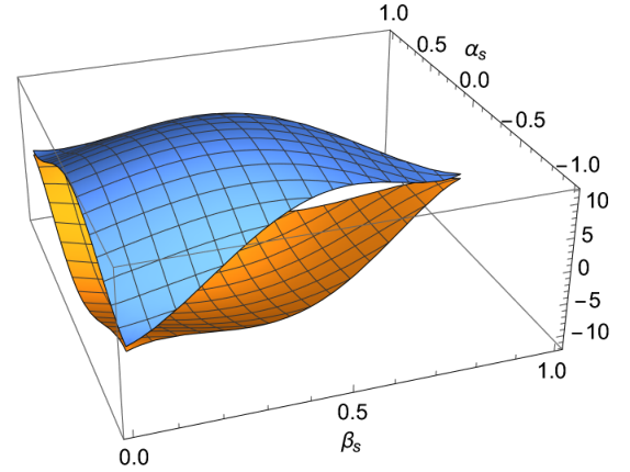
Finally, we plot the full shape of in Fig. 7 as a function of defined in (30) considering the same parameter values used in Fig. 3. There are several ways one can define the shape of bispectrum Chen:2010xka. One definition of the shape function is Chen:2010xka. In this paper, we stick to the shape function defined by the reduced bispectrum Kenton:2015lxa to represent the 3D plot in Fig. 7.
Following the discussion we presented towards the end of Sec. 4 (where we compared the interactions of curvature perturbation in our non-local theory with analogous interactions in local EFTs Chen:2010xka; Chen:2006xjb; Chen:2006nt) we can deduce that even though shapes of PNGs in non-local -like inflation appears to be a mixture of so-called squeezed, equilateral and orthogonal shape templates Chen:2010xka, we obtain here large non-trivial running of PNGs due to the strong scale dependencies due to non-localities which we discussed in Sec. 4. Therefore, the running of PNGs plays an important role in distinguishing PNGs in non-local -like inflation against local multifield non-canonical scalar fields inflation Chen:2010xka. This is similar to the running of tensor spectral index that was obtained in the our earlier work Koshelev:2022olc which acts as a distinguishable feature of non-local -like inflation against local EFTs at the level of the two-point tensor correlation function. However, we defer the detailed analysis of shape of PNGs for the full parameter space for future investigations.
6 Distinguishing generalized non-local -like inflation against EFT of scalar field inflation
In a broader view of developments in inflationary cosmology, we can notice that there are several ways one can construct a viable inflationary phase. Due to the lack of concrete understanding of UV-complete physics, numerous inflationary models were proposed in the past decades Martin:2013tda taking multiple approaches with different motivations towards UV-completion. In this respect, inflationary cosmology is hugely studied in the context of EFT involving single and multiple scalar fields of different nature Cheung:2007st; Senatore:2010wk; Kobayashi:2011nu. In view of inflationary observables related to 3-point correlations, we shall discuss how to distinguish EFT of several classes of inflationary models against the generalized non-local -like inflation we have studied in this paper. Note that distinguishing the generalized non-local -like inflation against the EFT of inflation was extensively discussed in Koshelev:2022olc.
Canonical single field inflation. This is the simplest framework of understanding inflation driven by a scalar field with the canonical kinetic term and a suitable potential. The successful models of this class are and Higgs inflation after the conformal transformation to the Einstein frame Akrami:2018odb. Independent of what is the choice of potential, this class of models always satisfy the tensor consistency relation and the Maldacena consistency relation. In our non-local gravity (4) these two consistency relations are violated (see Koshelev:2022olc and our result (31)). However, it has been widely understood that such models cannot be really single field ones because any attempt of embedding the models in a UV-complete framework introduce more degrees of freedom which eventually violate the consistency relation (although the new particles which appear in this way could be heavier than the inflaton) Linde:2014nna; Noumi:2012vr; Arkani-Hamed:2015bza; Lee:2016vti.
Non-canonical single field inflation. Non-canonical scalar field () is described by
| (40) |
where is a generic function of the canonical kinetic term and the field . This is a general action for a scalar field whose perturbations propagate with a sound speed . Because of this, non-canonical models of inflation can predict a peak in the equilateral limit, the tensor consistency relation is violated while tensor tilt remains unaffected by :
| (41) |
where the slow-roll parameter with subscript denotes the quantity in the canonical scalar field framework of inflation. With the Planck constraints (1), we get Akrami:2019izv. There are two ways we can distinguish our model from a non-canonical scalar one. One way is that in our case we modify tensor tilt and it becomes scale dependent (see Koshelev:2022olc). Another way is provided by the shape of PNGs, in the non-canonical model it is determined by the following interaction terms of curvature perturbation
| (42) | ||||
where is the curvature perturbation ( at super-Hubble scales) and are functions of slow-roll parameters Burrage:2011hd. If we compare these interaction terms with those we obtained in our theory (23), we can deduce that the large PNGs are of a possibility, and if the future observations will be powerful enough, we can distinguish our non-local gravity from non-canonical single field models of inflation.
Multifield inflation. Multifield inflation is basically an inflationary scenario driven by multiple scalar fields that leads to curvature and isocurvature perturbations during inflation Wands:2007bd. Therefore several classes of multifield inflation were studied in literature Byrnes:2014pja; Vennin:2015vfa. Due to the presence of isocurvature modes, curvature perturbation, if defined as being tangent to the background trajectory of inflaton fields in the field space, is generically not time-independent on super-Hubble scales66 6 Note, however, that there always exists another mode (a particular solution) of scalar perturbations in this case which is (approximately) time-independent in the super-Hubble regime Starobinsky:1994mh; Starobinsky:2001xq though it is not tangent to the inflaton background trajectory in the field space generically. Its existence can be traced to the fact that the FLRW scale factor is defined up to an arbitrary multiplier in the absence of spatial curvature, see Starobinsky:2001xq for more discussion. that leads to violation of the Maldacena consistency relation due to the classical evolution of fluctuations on such scales Vernizzi:2006ve; Wands:2007bd. As a result of this, the squeezed limit gives detectable level of non-Gaussianities. In our case we obtain detectable level of due to the non-local interactions of short and long wavelength modes which are quantum mechanical in nature (See Sec. 4 and Appendix B). Therefore, we generate in our model in a totally different way compared to multifield inflation. Furthermore, in the context of multifield inflation is almost scale independent Wands:2007bd. Moreover, multifield inflation with non-canonical scalar field predicts several types of PNGs (with large signatures in squeezed, equilateral and orthogonal limits) Gao:2008dt. In our case, we obtain various class of PNGs in a single field geometric construction of inflation. Particularly, in our case, we generate scale dependent PNGs with detectable running (see Sec. 4 and Sec. 5). Furthermore, tensor consistency relation is violated in multifield models of inflation due to the classical evolution of curvature perturbation in the presence of additional isocurvature fields Polarski:1995zn. But this feature can be distinguished from our case because we modify the tensor power spectrum that leads to corrections to the tensor spectral index and its running which are derived in Koshelev:2022olc.
EFT of single-field inflation.
EFT of single field inflation (EFT-SI) Cheung:2007st; Weinberg:2008hq is constructed to unify several single field models of inflation and aims to capture the signatures of UV-completion through the so-called EFT parameters that determine 2-point and 3-point inflationary correlations. It was elaborated in Koshelev:2022olc that the physics of two-point correlations in our generalized non-local gravity inflation with (4) cannot fall into the category of EFT-SI. The key EFT-SI parameters that affect both 2-point and 3-point correlations are the sound speeds of scalar (curvature) and tensor fluctuations which are slowly varying functions of time. In the EFT model considered in Creminelli:2014wna, in the original (disformal) frame, while in the Einstein frame obtained through the disformal transformation which changes the light cone. This leads to relation between scalar and tensor PNGs. In contrast to this, in our case of non-local gravity inflation we have both sounds speeds being unity and the scalar PNGs in our case are determined by the parameter space of the part of our full action (4) excluding the terms of the Weyl tensor. Therefore, we do get additional contributions which depend on additional parameter space for tensor PNGs that is the subject of our future investigation KKS2. This means that our geometric construction of inflation is indeed clearly distinguishable from that of the EFT-SI Cheung:2007st; Weinberg:2008hq. Focusing on the scalar PNGs in particular, the 3rd order action of EFT-SI prescribes
| (43) | ||||
The above action is derived in the limit then and it contains two interactions and associated with two parameters . These two interactions can be projected into equilateral and orthogonal shapes and the recent Planck data constrained them Akrami:2019izv. Comparing the interactions in (43) with our case (23), we can easily deduce that non-local gravity does contain more interactions and scale dependencies beyond the standard EFT-SI. Therefore, it would be of great interest to observationally probe (23) in the future CMB and LSS observations Meerburg:2019qqi.
EFTs of quasi-single field inflation (aka cosmological collider physics). This is a paradigm where there is one light scalar degree of freedom driving inflation interacting with heavy modes whose mass is of the order of the Hubble scale during inflation Chen:2010xka; Noumi:2012vr; Lee:2016vti. This framework of inflation is a natural set up in several UV-complete theories such as supergravity Bartolo:2018hjc; Hetz:2016ics; Aoki:2020zbj; Arkani-Hamed:2015bza. In this class of inflationary models equilateral, orthogonal and squeezed limit PNGs can be generated due to turns in the inflaton trajectory in the field space (that occur due to the presence of additional heavy fields). The crucial test of quasi-single field inflation is the shape of PNG that is scale dependent in the squeezed limit as follows Chen:2015lza
| (44) |
where is the function depending on which is the spin of the heavy particle, is the angle between long and short wavelenghth wave vectors and
| (45) |
with being the mass of the heavy particle. Depending on the mass of the heavy particle, we get different scale dependent features in the PNGs. This is a different scale dependence compared to what we have obtained in (31) where has scale dependence on the overall wave number rather than on the short and long wavelength modes in (44). This is the distinguishable feature of non-local theories from EFT of quasi-single field inflation.
7 Outlook
In this paper, we have computed and analyzed scalar PNGs which can be generated in the generalized non-local -like inflation and we provided detailed discussion about how our gravity framework of inflation goes beyond the several EFTs of inflation. Quantitative description of PNGs and their running is obtained, too. However, through scalar PNGs we only explored part of the action (4) which contributes to in the leading order. It is important to further understand tensor PNGs and cross-correlations that is the subject of our future investigation KKS2. Another direction to go forward is to compute 4-point correlations in the generalized non-local gravity inflation and check if the Suyama-Yamaguchi consistency relation Suyama:2007bg gets violated in non-local theories. Furthermore, it is interesting to explore the PNGs which can emerge if we couple matter degrees of freedom non-minimally and non-locally to gravity Draper:2020knh. Beyond these studies, it is theoretically very important to study formfactors of our gravity action (4) from a more fundamental point of view that can provide us with more robust and precise predictions.
Acknowledgements.
AK is supported by FCT Portugal investigator project IF/01607/2015. This research work was supported by grants UID/MAT/00212/2019, COST Action CA15117 (CANTATA). KSK acknowledges the support from JSPS and KAKENHI Grant-in-Aid for Scientific Research No. JP20F20320 and No. JP21H00069. KSK would like to thank the Royal Society for the Newton International Fellowship. AAS was supported by the RSF grant 21-12-00130. We would like to thank L. Buoninfante, A. De Felice, T. Noumi, A. Tokareva, T. Suyama and M. Yamaguchi for very useful discussions.Appendix A Computation of non-Gaussianities
In this section we compute the PNG contributions from the term which is cubic in Ricci scalar in (4).
| (46) | ||||
We can notice that (46) does not contain any terms involving second variations of Ricci scalar and the 3rd variations of such as
| (47) | ||||
since any such terms be multiplied by which become zero after imposing the on-shell condition (8). Further simplifying (46) using the following formula Koshelev:2020foq
| (48) |
we obtain
| (49) | ||||
where is the Hubble factor in conformal time. Here we have used the slow-roll approximation in the next to leading order in and made a substitution which solution in the quasi-dS approximation is
| (50) |
This follows from the computations in Koshelev:2022olc. We have also used the following relations which were derived using quasi-dS approximation (see Eqs (B.5) and (B.7) in Koshelev:2020foq):
| (51) | ||||
where denotes an analytic function of d’Alembertian . In (49) we carefully kept all terms up to the leading order in and neglected higher order contributions of treating . In our computation we re-sum contribution of all the infinite derivative terms. In the second line of (49), we made simplifications using (29). Since our case is single field inflation, perturbed modes deep inside the Hubble radius during inflation are evaluated at the Hubble radius exit since curvature perturbations remains constant on super-Hubble scales . So the 3-point correlations of do not evolve after that. Therefore, we evaluate the 3-point correlations at the moment when which is a conformal time after few e-foldings of the Hubble radius exit Pajer:2016ieg.
Here
| (52) |
| (53) | ||||
Considering the formfactors of the form (7) with the conditions imposed in (8), we can easily deduce that
| (54) |
in the limit of and . Note that since does not depend on the ratio , we found its contributions are far less than the contributions involving , especially for the operators of the form in (9).
Appendix B On violation of Maldacena consistency relation in non-local gravity
The goal of this section is to illustrate how the Maldacena consistency relation can be easily violated in non-local gravity. We provide here an explicit illustrative example from our study carried in this paper. It has been argued that the Maldacena consistency relation given by Maldacena:2002vr; Creminelli:2004yq; Creminelli:2011rh
| (55) |
cannot be violated in any single field slow-roll inflation with adiabatic vacuum initial conditions. The above relation was intuitively argued to be valid as follows. Since the curvature perturbation is constant on super-Hubble scales, the perturbed metric (say with wave-number ) in the so-called unitary gauge in which the inflaton perturbations can be put to zero Creminelli:2004yq; Creminelli:2011rh is approximated to be 77 7 C.f. Eq. (17) in Starobinsky:1982ee where is just up to a constant, and —— need not be small. In that paper, the synchronous gauge with additional conditions excluding two gauge modes was used but the resulting form of the metric in the leading approximation for appeared to be essentially the same as (56).
| (56) |
where the part of the scalar perturbations related to lapse and shift functions in the well-known Arnowitt-Deser-Misner (ADM) formalism Maldacena:2002vr are approximated to zero as they depend on the time and spatial derivatives of which is constant on the super-Hubble scales. Therefore, according to the standard intuitive proof Creminelli:2004yq; Creminelli:2011rh that is well supported by EFT of single-field inflation, the 3-point correlation in the squeezed limit can be decomposed as (using the simple Taylor expansion of 2-point correlation of short wavelength mode in the effective background metric (56))
| (57) | ||||
where are the power spectrum of mode and mode respectively. In deriving the above result, the trick of rescaling the spatial coordinates is used since can be treated as a constant on super-Hubble scales that was shown in Starobinsky:1982ee; Starobinsky:2001xq; Creminelli:2011rh. The above result is also concretely established and proved in local scalar-tensor theories.
In the context of non-local gravity we have seen that non-local interactions of curvature perturbations evade the above result (as we can witness from the expression of in (31)). To illustrate this, we consider a part of the action (4) with local terms and the non-local cubic scalar curvature term
| (58) |
Computing the second order perturbed action of (58) around the FLRW background obtained from (3), we can deduce that
| (59) |
where which is the result derived in Koshelev:2022olc. This means that at the second order perturbation level, (58) is exactly equivalent to local inflation and we can easily confirm that curvature perturbation is conserved on super-Hubble scales. But if we go to the interaction level, that is when we compute the bi-spectrum, we generate non-trivial contributions from the non-local interactions generated from the non-local cubic in scalar curvature term. These new contributions violate the Maldacena consistency relation as we can see from expression (31). Therefore, we can now precisely deduce that (58) is a counterexample to the intuitive derivation of the Maldacena consistency relation (57) because in the case of inflation with (58) we can see from the second order action that it is single field and slow-roll inflation since the background solutions is (3), but still we do violate the Maldacena consistency relation. This happens because the relations (29) lead to the enhancement of the interaction strength between the long wavelength mode and short wavelength modes beyond this order of slow-roll since .
So in summary, the proof (57) can only be valid in local theories, in particular two derivative theories, where the perturbed metric can be approximated as (56). Then one can Taylor expand 3-point correlation in the squeezed limit. In the case of non-local theory, one cannot apply this simple Taylor expansion because vertices come with formfactors of infinite derivative structure which we localize the action using the on-shell relations (29). This alters significantly the interaction picture and we get an exponential enhancement of 3-point vertices due to the structure of formfactors (6). However, we are well within the perturbative regime because the non-linear corrections to curvature perturbation in non-local -like inflation are still small and fluctuations are indeed very Gaussian as the current data suggest Akrami:2019izv.
References
- (1) A. S. Koshelev, K. S. Kumar, and A. A. Starobinsky, “Generalized non-local -like inflation,” arXiv:2209.02515 [hep-th], Accepted in JHEP.
- (2) A. A. Starobinsky, “A New Type of Isotropic Cosmological Models Without Singularity,” Phys. Lett. B 91 (1980) 99–102.
- (3) A. A. Starobinsky, “Nonsingular Model of the Universe with the Quantum Gravitational De Sitter Stage and its Observational Consequences,” in Proc. of the Second Seminar “Quantum Theory of Gravity”, Moscow Oct. 1981, INR Press, Moscow (1982), pp. 58–72.
- (4) A. A. Starobinsky, “The Perturbation Spectrum Evolving from a Nonsingular Initially De-Sitter Cosmology and the Microwave Background Anisotropy,” Sov. Astron. Lett. 9 (1983) 302–304.
- (5) A. Vilenkin, “Classical and Quantum Cosmology of the Starobinsky Inflationary Model,” Phys. Rev. D 32 (1985) 2511.
- (6) M. B. Mijic, M. S. Morris, and W.-M. Suen, “The Cosmology: Inflation Without a Phase Transition,” Phys. Rev. D 34 (1986) 2934.
- (7) K.-i. Maeda, “Inflation as a Transient Attractor in Cosmology,” Phys. Rev. D 37 (1988) 858.
- (8) Planck Collaboration, Y. Akrami et al., “Planck 2018 results. X. Constraints on inflation,” arXiv:1807.06211 [astro-ph.CO].
- (9) BICEP, Keck Collaboration, P. A. R. Ade et al., “Improved Constraints on Primordial Gravitational Waves using Planck, WMAP, and BICEP/Keck Observations through the 2018 Observing Season,” Phys. Rev. Lett. 127 no. 15, (2021) 151301, arXiv:2110.00483 [astro-ph.CO].
- (10) C. Cheung, P. Creminelli, A. L. Fitzpatrick, J. Kaplan, and L. Senatore, “The Effective Field Theory of Inflation,” JHEP 03 (2008) 014, arXiv:0709.0293 [hep-th].
- (11) S. Weinberg, “Effective Field Theory for Inflation,” Phys. Rev. D 77 (2008) 123541, arXiv:0804.4291 [hep-th].
- (12) X. Chen, “Primordial Non-Gaussianities from Inflation Models,” Adv. Astron. 2010 (2010) 638979, arXiv:1002.1416 [astro-ph.CO].
- (13) Z. Kenton and D. J. Mulryne, “The squeezed limit of the bispectrum in multi-field inflation,” JCAP 10 (2015) 018, arXiv:1507.08629 [astro-ph.CO].
- (14) Planck Collaboration, Y. Akrami et al., “Planck 2018 results. IX. Constraints on primordial non-Gaussianity,” Astron. Astrophys. 641 (2020) A9, arXiv:1905.05697 [astro-ph.CO].
- (15) T. Kobayashi, M. Yamaguchi, and J. Yokoyama, “Generalized G-inflation: Inflation with the most general second-order field equations,” Prog. Theor. Phys. 126 (2011) 511–529, arXiv:1105.5723 [hep-th].
- (16) E. Komatsu and et al, “Non-Gaussianity as a Probe of the Physics of the Primordial Universe and the Astrophysics of the Low Redshift Universe,” Science White Paper submitted to the Cosmology and Fundamental Physics (CFP) Science Frontier Panel of the Astro 2010 Decadal Survey (2009) , arXiv:0902.4759.
- (17) S. Bahrami and E. E. Flanagan, “Primordial non-Gaussianities in single field inflationary models with non-trivial initial states,” JCAP 10 (2014) 010, arXiv:1310.4482 [astro-ph.CO].
- (18) Planck Collaboration, Y. Akrami et al., “Planck 2018 results. IX. Constraints on primordial non-Gaussianity,” arXiv:1905.05697 [astro-ph.CO].
- (19) X. Chen, M.-x. Huang, S. Kachru, and G. Shiu, “Observational signatures and non-Gaussianities of general single field inflation,” JCAP 0701 (2007) 002, arXiv:hep-th/0605045 [hep-th].
- (20) X. Chen, “Running non-Gaussianities in DBI inflation,” Phys. Rev. D 72 (2005) 123518, arXiv:astro-ph/0507053.
- (21) P. Creminelli, G. D’Amico, M. Musso, J. Norena, and E. Trincherini, “Galilean symmetry in the effective theory of inflation: new shapes of non-Gaussianity,” JCAP 02 (2011) 006, arXiv:1011.3004 [hep-th].
- (22) L. Senatore and M. Zaldarriaga, “The Effective Field Theory of Multifield Inflation,” JHEP 04 (2012) 024, arXiv:1009.2093 [hep-th].
- (23) N. Arkani-Hamed and J. Maldacena, “Cosmological Collider Physics,” arXiv:1503.08043 [hep-th].
- (24) X. Chen and Y. Wang, “Quasi-Single Field Inflation and Non-Gaussianities,” JCAP 1004 (2010) 027, arXiv:0911.3380 [hep-th].
- (25) J. Martin, C. Ringeval, and V. Vennin, “Encyclopædia Inflationaris,” Phys. Dark Univ. 5-6 (2014) 75–235, arXiv:1303.3787 [astro-ph.CO].
- (26) A. S. Koshelev, K. Sravan Kumar, and A. A. Starobinsky, “Generalized -like inflation and tensor non-Gaussianities,” arXiv:2211.XXXX [hep-th].
- (27) A. S. Koshelev, K. Sravan Kumar, A. Mazumdar, and A. A. Starobinsky, “Non-Gaussianities and tensor-to-scalar ratio in non-local R2-like inflation,” JHEP 06 (2020) 152, arXiv:2003.00629 [hep-th].
- (28) Planck Collaboration, P. A. R. Ade et al., “Planck 2015 results. XVII. Constraints on primordial non-Gaussianity,” Astron. Astrophys. 594 (2016) A17, arXiv:1502.01592 [astro-ph.CO].
- (29) X. Gao, “Primordial Non-Gaussianities of General Multiple Field Inflation,” JCAP 0806 (2008) 029, arXiv:0804.1055 [astro-ph].
- (30) C. T. Byrnes, “Lecture notes on non-Gaussianity,” Astrophys. Space Sci. Proc. 45 (2016) 135–165, arXiv:1411.7002 [astro-ph.CO].
- (31) F. Oppizzi, M. Liguori, A. Renzi, F. Arroja, and N. Bartolo, “CMB constraints on running non-Gaussianity,” JCAP 05 (2018) 045, arXiv:1711.08286 [astro-ph.CO].
- (32) P. D. Meerburg et al., “Primordial Non-Gaussianity,” arXiv:1903.04409 [astro-ph.CO].
- (33) D. Karagiannis, A. Lazanu, M. Liguori, A. Raccanelli, N. Bartolo, and L. Verde, “Constraining primordial non-Gaussianity with bispectrum and power spectrum from upcoming optical and radio surveys,” Mon. Not. Roy. Astron. Soc. 478 no. 1, (2018) 1341–1376, arXiv:1801.09280 [astro-ph.CO].
- (34) E. Castorina, Y. Feng, U. Seljak, and F. Villaescusa-Navarro, “Primordial non-Gaussianities and zero bias tracers of the Large Scale Structure,” Phys. Rev. Lett. 121 no. 10, (2018) 101301, arXiv:1803.11539 [astro-ph.CO].
- (35) J. B. Muñoz, Y. Ali-Haïmoud, and M. Kamionkowski, “Primordial non-gaussianity from the bispectrum of 21-cm fluctuations in the dark ages,” Phys. Rev. D 92 no. 8, (2015) 083508, arXiv:1506.04152 [astro-ph.CO].
- (36) T. Flöss, T. de Wild, P. D. Meerburg, and L. V. E. Koopmans, “The Dark Ages’ 21-cm Trispectrum,” arXiv:2201.08843 [astro-ph.CO].
- (37) J. M. Maldacena, “Non-Gaussian features of primordial fluctuations in single field inflationary models,” JHEP 05 (2003) 013, arXiv:astro-ph/0210603 [astro-ph].
- (38) A. De Felice and S. Tsujikawa, “Primordial non-Gaussianities in general modified gravitational models of inflation,” JCAP 1104 (2011) 029, arXiv:1103.1172 [astro-ph.CO].
- (39) E. Komatsu and D. N. Spergel, “Acoustic signatures in the primary microwave background bispectrum,” Phys. Rev. D63 (2001) 063002, arXiv:astro-ph/0005036 [astro-ph].
- (40) T. Takahashi, “Primordial non-Gaussianity and the inflationary Universe,” PTEP 2014 no. 6, (2014) 06B105.
- (41) X. Chen, R. Easther, and E. A. Lim, “Large Non-Gaussianities in Single Field Inflation,” JCAP 0706 (2007) 023, arXiv:astro-ph/0611645 [astro-ph].
- (42) D. Babich, P. Creminelli, and M. Zaldarriaga, “The Shape of non-Gaussianities,” JCAP 0408 (2004) 009, arXiv:astro-ph/0405356 [astro-ph].
- (43) D. Seery and J. E. Lidsey, “Primordial non-Gaussianities in single field inflation,” JCAP 0506 (2005) 003, arXiv:astro-ph/0503692 [astro-ph].
- (44) K. Sravan Kumar, S. Maheshwari, and A. Mazumdar, “Perturbations in higher derivative gravity beyond maximally symmetric spacetimes,” Phys. Rev. D100 no. 6, (2019) 064022, arXiv:1905.03227 [gr-qc].
- (45) J. R. Fergusson and E. P. S. Shellard, “The shape of primordial non-Gaussianity and the CMB bispectrum,” Phys. Rev. D 80 (2009) 043510, arXiv:0812.3413 [astro-ph].
- (46) D. Seery, “Infrared effects in inflationary correlation functions,” Class. Quant. Grav. 27 (2010) 124005, arXiv:1005.1649 [astro-ph.CO].
- (47) E. Pajer, G. L. Pimentel, and J. V. S. Van Wijck, “The Conformal Limit of Inflation in the Era of CMB Polarimetry,” JCAP 1706 no. 06, (2017) 009, arXiv:1609.06993 [hep-th].
- (48) C. Burrage, R. H. Ribeiro, and D. Seery, “Large slow-roll corrections to the bispectrum of noncanonical inflation,” JCAP 07 (2011) 032, arXiv:1103.4126 [astro-ph.CO].
- (49) A. De Felice and S. Tsujikawa, “f(R) theories,” Living Rev. Rel. 13 (2010) 3, arXiv:1002.4928 [gr-qc].
- (50) P. Creminelli and M. Zaldarriaga, “Single field consistency relation for the 3-point function,” JCAP 10 (2004) 006, arXiv:astro-ph/0407059.
- (51) A. Linde, “Inflationary Cosmology after Planck 2013,” in Proceedings, 100th Les Houches Summer School: Post-Planck Cosmology: Les Houches, France, July 8 - August 2, 2013, pp. 231–316. 2015. arXiv:1402.0526 [hep-th]. https://inspirehep.net/record/1280019/files/arXiv:1402.0526.pdf.
- (52) T. Noumi, M. Yamaguchi, and D. Yokoyama, “Effective field theory approach to quasi-single field inflation and effects of heavy fields,” JHEP 06 (2013) 051, arXiv:1211.1624 [hep-th].
- (53) H. Lee, D. Baumann, and G. L. Pimentel, “Non-Gaussianity as a Particle Detector,” JHEP 12 (2016) 040, arXiv:1607.03735 [hep-th].
- (54) D. Wands, “Multiple field inflation,” Lect. Notes Phys. 738 (2008) 275–304, arXiv:astro-ph/0702187.
- (55) V. Vennin, K. Koyama, and D. Wands, “Encyclopædia curvatonis,” JCAP 11 (2015) 008, arXiv:1507.07575 [astro-ph.CO].
- (56) A. A. Starobinsky and J. Yokoyama, “Density fluctuations in Brans-Dicke inflation,” in Proc. of 4th Workshop on General Relativity and Gravitation, eds. K. Nakao et al. (Kyoto University, 1995), pp. 381–390. arXiv:gr-qc/9502002.
- (57) A. A. Starobinsky, S. Tsujikawa, and J. Yokoyama, “Cosmological perturbations from multifield inflation in generalized Einstein theories,” Nucl. Phys. B 610 (2001) 383–410, arXiv:astro-ph/0107555.
- (58) F. Vernizzi and D. Wands, “Non-gaussianities in two-field inflation,” JCAP 05 (2006) 019, arXiv:astro-ph/0603799.
- (59) D. Polarski and A. A. Starobinsky, “Structure of primordial gravitational waves spectrum in a double inflationary model,” Phys. Lett. B 356 (1995) 196–204, arXiv:astro-ph/9505125.
- (60) P. Creminelli, J. Gleyzes, J. Noreña, and F. Vernizzi, “Resilience of the standard predictions for primordial tensor modes,” Phys. Rev. Lett. 113 no. 23, (2014) 231301, arXiv:1407.8439 [astro-ph.CO].
- (61) N. Bartolo, D. M. Bianco, R. Jimenez, S. Matarrese, and L. Verde, “Supergravity, -attractors and primordial non-Gaussianity,” JCAP 10 (2018) 017, arXiv:1805.04269 [astro-ph.CO].
- (62) A. Hetz and G. A. Palma, “Sound Speed of Primordial Fluctuations in Supergravity Inflation,” Phys. Rev. Lett. 117 no. 10, (2016) 101301, arXiv:1601.05457 [hep-th].
- (63) S. Aoki and M. Yamaguchi, “Disentangling mass spectra of multiple fields in cosmological collider,” JHEP 04 (2021) 127, arXiv:2012.13667 [hep-th].
- (64) X. Chen, M. H. Namjoo, and Y. Wang, “Quantum Primordial Standard Clocks,” JCAP 02 (2016) 013, arXiv:1509.03930 [astro-ph.CO].
- (65) T. Suyama and M. Yamaguchi, “Non-Gaussianity in the modulated reheating scenario,” Phys. Rev. D 77 (2008) 023505, arXiv:0709.2545 [astro-ph].
- (66) T. Draper, B. Knorr, C. Ripken, and F. Saueressig, “Graviton-Mediated Scattering Amplitudes from the Quantum Effective Action,” JHEP 11 (2020) 136, arXiv:2007.04396 [hep-th].
- (67) P. Creminelli, G. D’Amico, M. Musso, and J. Norena, “The (not so) squeezed limit of the primordial 3-point function,” JCAP 11 (2011) 038, arXiv:1106.1462 [astro-ph.CO].
- (68) A. A. Starobinsky, “Dynamics of Phase Transition in the New Inflationary Universe Scenario and Generation of Perturbations,” Phys. Lett. B 117 (1982) 175–178.