Potential scientific synergies in weak lensing studies between the CSST and Euclid space probes
Abstract
Aims. With the next generation of large surveys coming to the stage of observational cosmology soon, it is important to explore their potential synergies and to maximise their scientific outcomes. In this study, we aim to investigate the complementarity of the two upcoming space missions Euclid and the China Space Station Telescope (CSST), focusing on weak gravitational lensing for cosmology. In particular, we analyse the photometric redshift (photo-) measurements by combining NUV, bands from CSST with VIS, bands from Euclid and other optical bands from the ground-based Vera C. Rubin Observatory Legacy Survey of Space and Time (LSST) and Dark Energy Survey. The advantages of combining the two space observational data in simplifying image deblending are also studied. For Euclid, weak lensing measurements use the broad optical wavelength range of 550-900 nm, for which chromatic point-spread function (PSF) effects are significant. For this, the CSST narrow-band data in the optical can provide valuable information for Euclid to obtain more accurate PSF measurements, and to calibrate the colour and colour-gradient biases for galaxy shear measurements.
Methods. We create image simulations, using the Hubble Deep UV data as the input catalogue, for different surveys, and quantify the photo- performance using EAZY template fitting. For blending analyses, we employ high-resolution HST-ACS CANDELS F606W and F814W data to synthesize mock simulated data for Euclid, CSST, and an LSST-like survey. We analyse the blending fraction for different cases, and the blending effects on galaxy photometric measurements. Furthermore, we demonstrate that CSST can provide a large enough number of high signal-to-noise ratio multi-band galaxy images to calibrate the colour-gradient biases for Euclid.
Results. The sky coverage of Euclid lies entirely within the CSST footprint. The combination of Euclid with CSST data can thus be done more uniformly than with the various ground-based data that are part of the Euclid survey. Our studies show that by combining Euclid and CSST, we can reach a photo- precision of , and an outlier fraction of at the nominal depth of the Euclid Wide Survey ( AB mag). For CSST, including the Euclid bands reduces the overall photo- outlier fraction from to . For , the improvements are even more significant. Because of the similarly high resolutions, the data combination of Euclid and CSST can be relatively straightforward for photometry measurements. On the other hand, to include ground-based data, sophisticated deblending utilizing priors from high-resolution space observations is demanded. The multi-band data from CSST are very helpful in controlling the chromatic PSF effect for Euclid VIS shear measurements. The colour-gradient bias for Euclid galaxies with different bulge-to-total flux ratio at different redshifts can be well calibrated to the level of using galaxies from the CSST deep survey.
Key Words.
dark energy – dark matter – Gravitational lensing: weak – large-scale structure of the Universe – surveys – telescopes1 Introduction
Rapid observational developments in the past few decades have changed cosmological studies dramatically from lacking of data to data driven. Consequently, our understanding about the Universe has increasingly deepened, leading to the emergence of the cosmic concordance model. According to it, the two dark components, namely dark matter and dark energy, play essential roles in shaping the present Universe. On the other hand, however, their nature is still to be understood, which is one of the greatest challenges in the research of fundamental physics (Weinberg et al. 2013, e.g.).
The dark components affect both the global cosmic expansion and the formation and evolution of large-scale structures (LSS). Thus observables from both aspects are sought to as sensitive probes (Albrecht et al. 2006). Among others, the weak lensing (WL) effect has been widely recognized as one of the major tools in cosmological studies (Fu & Fan 2014; Kilbinger 2015; Mandelbaum 2018). Arising from the gravitational light deflection by foreground LSS, WL leads to tiny shape distortions and flux changes of background objects (Bartelmann & Schneider 2001). By observing those changes, we therefore can extract the underlying matter distribution in an unbiased way. Furthermore, WL depends on the distances between observer, foreground lenses, and background sources, and thus is sensitive to the global expansion of the Universe. On the other hand, however, WL cosmological studies are observationally challenging because of the weakness of the signals. The past twenty years witnessed great improvements in high-precision photometric surveys, which have made WL one of the fastest developing areas in cosmological observations.
Represented by CFHTLenS (Fu et al. 2008; Heymans et al. 2012; Kilbinger et al. 2013), Stage-II (Albrecht et al. 2006) surveys demonstrated fully the observational feasibility of WL cosmological studies. We are now in the Stage-III era with a number of surveys observing a few thousand square degrees of sky area, resulting in high quality shear samples containing to galaxies (Kuijken et al. 2015; Dark Energy Survey Collaboration et al. 2016; Aihara et al. 2018). These surveys have already provided valuable cosmological constraints, complementary to other probes such as galaxy clustering or cosmic microwave background (CMB) anisotropies by breaking the degeneracy of different cosmological parameters (Heymans et al. 2021; Tröster et al. 2021; Abbott et al. 2022; Hikage et al. 2019). In particular, they reveal a potential discrepancy within the CDM paradigm between the measurements from low-redshift large-scale structures including WL and galaxy clustering, and from the CMB observations (Hildebrandt et al. 2017; Hildebrandt et al. 2020; Heymans et al. 2021; Lemos et al. 2021; Planck Collaboration et al. 2020). Here and and are the present dimensionless matter density and the root-mean-square of the linearly-extrapolated matter density fluctuations over a top-hat scale of with being the dimensionless Hubble constant in units of . This has stimulated great attentions because it may imply new physics beyond our current understanding. On the other hand, however, from the current surveys, the difference is marginal with a low statistical significance of . It is still under debate if this is a real problem for the CDM cosmology (Abbott et al. 2022, e.g.).
To further enhance the power of cosmological constraints, Stage-IV surveys will be in operation within the next five years or so. These include the ground-based Vera C. Rubin Observatory Legacy Survey of Space and Time (Ivezić et al. 2019, LSST;), the space-based Euclid telescope (Laureijs et al. 2011), the Roman Space Telescope (Spergel et al. 2015, Roman;), and the China Space Station Telescope (Zhan 2011; Zhan 2018; Fan 2018; Gong et al. 2019; Zhan 2021, CSST;). These surveys target at high precision WL measurements for over a billion galaxies, an order of magnitude more than that of the current surveys. Consequently, the statistical power will be greatly increased. The problem, if it indeed exists, will show up unambiguously. Utilising WL and galaxy clustering statistical analyses, the constraints on the equation-of-state parameters and of dark energy can expectedly reach the precision of about and , respectively, about an order of magnitude tighter than that from the current survey studies (Euclid Collaboration et al. 2020a; Gong et al. 2019, e.g.). Here the equation of state of dark energy is assumed to be and with and the pressure and energy density , and the redshift. This will allow us to answer the very fundamental question with high statistical significance if the dark energy is in the form of cosmological constant or dynamical in nature.
The full realisation of the statistical capability of Stage IV surveys requires stringent controls on different systematics. For WL cosmological studies, the multiplicative shear measurement bias needs to be known to an accuracy of about . The photometric redshift (photo-) bias and scatter in different redshift bins should be less than and , respectively. The catastrophic outlier fraction of photo-s needs to be less than (Laureijs et al. 2011, e.g.). Different Stage-IV surveys have different designs. How to utilise their data to improve the control of systematics and thus to maximise the science outcome is an important task that has triggered significant studies (Jain et al. 2015; Rhodes et al. 2017; Chary et al. 2020; Eifler et al. 2021; Guy et al. 2022).
The Euclid and the CSST are both space-based projects with common scientific objectives. Their high spatial resolutions allow accurate WL shear measurements for galaxies of small sizes unachievable from ground-based observations. The fraction of image blending, a serious issue for deep ground-based surveys, is much reduced in the two space surveys, which can benefit significantly the accurate shear and photo- measurements. The Euclid imaging survey has one broad optical VIS band from 550 nm to 900 nm for accurate WL shear measurements, and three near infrared (NIR) bands of , and for photo- estimates (Laureijs et al. 2011). To obtain photo-s with the required accuracies, the Euclid needs external multi-band optical data (Rhodes et al. 2017; Euclid Collaboration et al. 2020b; Guinot et al. 2022, e.g.). For shear measurements using the broad VIS band, the wavelength-dependent point-spread function (PSF) and the differences between the spectral energy distribution (SED) of stars and galaxies can lead to significant biases for galaxy shear measurements (Eriksen & Hoekstra 2018, e.g.). In addition, the spatial variation of colours across a galaxy can also induce a colour-gradient shear bias. They need to be carefully dealt with. The CSST has seven optical bands of NUV, and (Zhan 2021) for imaging surveys, very complementary to the Euclid. For photo- measurements, the CSST can provide external optical data necessary for the Euclid. On the other hand, the inclusion of the Euclid NIR data can significantly improve the CSST photo-s at redshift . The similar spatial resolutions of the two space missions make the data combinations less complicated than combining space- and ground-based data. The CSST multi-band data in optical can also be very helpful in calibrating the colour related shear measurement biases for the Euclid.
Seeing the great complementarities, in this paper, we present the first study aiming to explore the potential synergies between the Euclid and the CSST with a focus on WL cosmology. This paper is organized as follows. Sect. 2 describes the characteristics of the CSST and the Euclid, respectively. In Sect. 3, we present the possible synergies for WL studies. We briefly mention a few other aspects of cosmological studies that can benefit from the joint analyses of the two missions in Sect. 4. We discuss our results in Sect. 5.
2 Introduction to the CSST and the Euclid

2.1 CSST
CSST is a major science project of the China Manned Space Program and is planned to be launched around 2024 (Zhan 2011; Gong et al. 2019). The telescope is a 2m Cook-type off-axis three-mirror anastigmat (TMA) system with five first-generation instruments: a survey camera, a terahertz receiver, a multichannel imager, an integral field spectrograph, and a cool planet imaging coronagraph (Zhan 2021). A fold mirror is placed near the exit pupil to direct light to different instruments. The pointing accuracy of CSST is specified to be with stability of () over 300 s with/without guide stars. The roll angle accuracy is with stability () over 300 s. The jitter requirement is ().
The wide-field survey camera will be used to carry out a large-area high-resolution multi-band imaging and slitless spectroscopic survey. The imaging survey data will enable precision cosmological studies with multiple probes, including weak lensing, strong lensing, and galaxy clustering. The spectroscopic survey will map the galaxy redshift distribution for extracting cosmic signals of the baryon acoustic oscillation and the redshift-space distortion at different redshifts. The high-quality survey data will also enable a wide range of astrophysical studies, from galaxy formation and evolution to solar system objects.
The primary focal plane of the survey camera is shown in the left panel of Fig. 1. It is segmented into tiles with for multi-band imaging, and for slitless spectroscopic observations. They are arranged into a array. The field-of-view (FOV) is . Covering the wavelength range from to nm, the imaging bands consist of NUV, u, g, r, i, z and y, and the pixel scale is . The slitless spectroscopy bands include GU (255–400nm), GV (400–620nm), and GI (620–1000nm) with the same pixel scale. These different bands are distributed in the focal plane, with each occupying 2 or 4 segments. The targeted angular resolution for imaging observations is about in terms of the radius at 80% encircled energy (). The resolution has a slight band variation. The angular resolution for the slitless spectroscopy is /pixel, and the average spectral resolution is 200.
The planned surveys for both imaging and spectroscopy include, but are not limited to, a wide-field survey over about 17 500 deg2 sky area and a deep-field survey of about 400 deg2. The wide-field imaging survey will reach an average limiting magnitude better than 25.5 AB mag at 5 for point sources. For the spectroscopic survey, it is 23.7 mag. They are about 1.2 mag deeper for the deep-field survey. For WL studies from the wide-field survey, the expected galaxy number density can reach , and the median redshift is about .
Around the primary focal plane, a flux calibration unit and a NIR unit will be equipped. The flux calibration unit is designed to assist flux calibration in r-band by observing stars that will be too bright for the main survey. This will be achieved by placing the detector off the focus, allowing a saturation limit 4 mag brighter than that of the main survey. The NIR unit has 8 HgCdTe detectors in two groups, imaging and slitless spectroscopy. Each group has four detectors, two in the -band (0.9–1.3m) and two in -band (1.3–1.7m). Each detector has a FOV of ( of the detectors in the primary focal plane). The limiting magnitude for NIR imaging is mag in and mag in (150 s exposure, point source 5). The spectral resolution for slitless spectroscopy is , and point sources brighter than mag are detectable.
2.2 Euclid
Euclid (Laureijs et al. 2011) is an ESA M-class astrophysics and cosmology mission with a currently expected launch early 2023. For cosmology it will employ two primary probes, weak lensing and galaxy clustering, aiming to constrain dark energy properties with a figure of merit (Albrecht et al. 2006, e.g.), the exponent of the growth factor with a precision of , the sum of the neutrino masses with a precision of eV, and initial conditions of cosmic structure formation parameterised by to a precision of in combination with Planck CMB observations (Planck Collaboration et al. 2020; Euclid Collaboration et al. 2020a).
Euclid’s payload includes a 1.2m Korsch telescope equipped with two instruments, which simultaneously probe a common FOV of deg2. The optical VIS imager comprises 36 4k4k CCDs with / pixel. The Near-Infrared Spectrograph and Photometer (NISP) includes 16 arrays of 2k2k NIR-sensitive HgCdTe detectors with a pixel scale of . The middle and right panels of Fig. 1 show the focal planes of the two instruments. Euclid will survey 15 000 deg2 of the extragalactic sky avoiding the ecliptic plane due to increased zodiacal background in its Wide Survey and use step and stare mode with four dither pointings per step (Euclid Collaboration et al. 2022), plus 40 deg2 split over three deep fields11 1 https://www.cosmos.esa.int/web/euclid/euclid-survey with a depth increase by 2 mag.
NISP will obtain NIR imaging in , , and bands for photometric redshifts reaching 24 AB mag at 5 for point sources in the Wide Survey, plus slitless spectroscopy for galaxy clustering studies with a flux limit of erg cm-2 s-1 at for a diameter source.
VIS images will be taken in a broad – nm optical bandpass, reaching AB mag at 10 for galaxies with a size larger than 1.25 times the full width at half-maximum (FWHM) of the PSF. These data will be used to obtain galaxy shape measurements for weak lensing. In order to optimise the thermal stability and minimise temporal PSF variations for WL measurements, Euclid will observe from an orbit around the Sun-Earth Lagrange point L2. In addition, the variation of space-craft orientations with respect to the Sun will be limited to maximise PSF stability.
For the WL analysis, galaxies need to be split into tomographic bins using photometric redshift. For this, the Euclid data need to be combined with depth-matched multi-band optical observations, such as, from ground-based wide-field imaging surveys. These optical colour measurements are also needed to account for the colour-dependence of the diffraction-limited VIS PSF when modelling the PSF and measuring galaxy shapes (Cypriano et al. 2010; Eriksen & Hoekstra 2018). Shape measurements based on VIS will also require at least statistical corrections for the impact of galaxy colour gradients, which cannot be constrained individually from seeing-limited colour measurements (Voigt et al. 2012; Semboloni et al. 2013; Er et al. 2018).
3 Synergies for weak lensing science
In this section, we present the aspects in WL studies that can benefit from the joint analyses of the two missions.
3.1 Photometric redshifts
Accurate photo- measurements have become an indispensable part of weak lensing cosmology (Hildebrandt et al. 2010; Newman et al. 2015; Tanaka et al. 2018; Hildebrandt et al. 2021; Myles et al. 2021). The accuracy of photo- depends critically on the wavelength coverage and the filter bands employed in observations (Liu et al. 2017; Salvato et al. 2019). While optical bands are the core for photo- measurements, the inclusion of NIR bands is important to improve photo- for . Additionally, observations of and NUV bands at shorter wavelength can reduce the low-redshift outlier fraction by correctly disentangling the break and the redshifted Lyman break and Lyman line features (Rafelski et al. 2015).
CSST has seven filters consisting of NUV, . For Euclid, there is a single broad VIS band in the optical from 550-900 nm mainly for galaxy weak lensing shear measurements, and three NIR bands for photo- determination. The optimal utilization of the data from the two surveys can improve the photo- accuracy profoundly. In addition, the two space-based surveys have similar resolutions in optical bands, and thus the complexity in image deblending can be much less than that of combining space- and ground-based data.
Below we present our investigations on the photo- accuracy by utilizing CSST and Euclid observations. For comparison, we also study combinations of Euclid and ground-based observations that match the characteristics of the LSST (Ivezić et al. 2019) and the Stage-III Dark Energy Survey (Dark Energy Survey Collaboration et al. 2016, DES;). Table 1 shows the band information and the designed performance parameters of each survey used in our analyses. In our study here, four setups are considered for the photo- analyses: 1) CSST-only setup containing 7 optical bands, 2) Euclid+CSST setup with 11 optical and NIR bands, 3) Euclid+LSST-like setup having 10 optical and NIR bands, and 4) Euclid+DES-like setup consisting of 9 optical and NIR bands. As stated in Euclid Collaboration et al. 2020b, the Euclid WL shear sample is defined by a set of galaxies with VIS-band signal-to-noise ratio higher than 10, corresponding to the magnitude depth of mag, and being not flagged as having bad photometry or active galactic nuclei (AGNs). In addition, concerning the reliability of photo- estimates, the Euclid shear sample is set to be in the range of . In this work, we apply the same criteria to analyze the photo- accuracy. Detailed image simulation and photo- measurements are presented as follows.
3.1.1 Method and simulations
For the photo- analyses here, we generate simulated mocks based on the Hubble Deep UV (HDUV) Legacy Survey GOODS-N/CANDELS-Deep data catalogue (Oesch et al. 2018). The sky area is centred on (RA, DEC)=(, ). The source detection of the HDUV catalogue is based on the coadded images of the three HST WFC3 bands , and with an average PSF (Skelton et al. 2014). This is comparable to the resolution of the Euclid VIS band and of the CSST bands, and thus this catalogue is very suitable for our studies. In contrast, for the COSMOS2015 sample (Laigle et al. 2016) that has been extensively used in photo- studies (Rhodes et al. 2017; Cao et al. 2018, e.g.), the source detection is primarily based on UltraVISTA NIR bands (McCracken et al. 2012) and Subaru band (Taniguchi et al. 2015). These images have PSFs with a typical value of . This lower resolution resulted in a lower number density of galaxies in the COSMOS2015 catalogue than that of HDUV. For our studies here concerning the space-based Euclid and CSST, photo- analyses based on the high-resolution HDUV catalogue are optimal.
With the HDUV catalogue as the input, we use GALSIM, a flexible framework to simulate galaxy images (Rowe et al. 2015), to perform image simulations for different considered bands at the pixel level. The procedures are as follows.
| Telescope/ | Band | Detection Limit | Pixel Scale | PSF Size | ||
| Project | (Å) | (Å) | (mag) | (arcsec) | (arcsec) | |
| CSST$a$$a$footnotetext: | NUV | 2880 | 694 | 25.4 | 0.135 | |
| u | 3726 | 866 | 25.4 | 0.135 | ||
| g | 4734 | 1455 | 26.3 | 0.135 | ||
| r | 6107 | 1417 | 26.0 | 0.074 | 0.135 | |
| i | 7548 | 1465 | 25.9 | 0.145 | ||
| z | 8975 | 1082 | 25.2 | 0.165 | ||
| y | 9606 | 542 | 24.4 | 0.165 | ||
| Euclid$b$$b$footnotetext: | VIS | 6726 | 3699 | 24.5 | 0.1 | 0.18 |
| 10 678 | 2665 | 24.0 | 0.3 | 0.62 | ||
| 13 333 | 4052 | 24.0 | 0.3 | 0.63 | ||
| 17 328 | 5023 | 24.0 | 0.3 | 0.70 | ||
| LSST$c$$c$footnotetext: | u | 3734 | 623 | 26.1 | 0.81 | |
| g | 4731 | 1427 | 27.4 | 0.77 | ||
| r | 6139 | 1359 | 27.5 | 0.73 | ||
| i | 7487 | 1247 | 26.8 | 0.2 | 0.69 | |
| z | 8671 | 1022 | 26.1 | 0.68 | ||
| y | 9677 | 855 | 24.9 | 0.71 | ||
| DES$d$$d$footnotetext: | g | 4734 | 1295 | 24.7 | 1.11 | |
| r | 6342 | 1485 | 24.4 | 0.95 | ||
| i | 7748 | 1480 | 23.8 | 0.263 | 0.88 | |
| z | 9139 | 1475 | 23.1 | 0.83 | ||
| y | 9880 | 660 | 21.7 | 0.90 |
(1) We select galaxies in the HDUV sample by setting the parameter use_phot==1, which combines a number of criteria described in Skelton et al. 2014, such as not being a star, not being close to a bright star, etc.. In real observations, bright stars can affect the photometry of nearby galaxies and may lead to catastrophic photo- measurements. Therefore, in WL studies bright stars need to be masked with specified radii to reduce their effects (Kuijken et al. 2015, e.g.). Here we rely on the flag of use_phot==1 in the original HDUV catalogue that already excludes galaxies close to bright stars. Therefore the photometry of the selected galaxies should not be affected significantly (Skelton et al. 2014). In addition, in our simulation analyses, we only use the position and the SED information of the galaxies, and their images are generated with GALSIM. We therefore expect negligible impacts from bright stars on our studies. For real Euclid and CSST data processing, however, this issue needs to be carefully dealt with, which is beyond the scope of the current paper. After applying the cut, the resulting total number of galaxies is . For each galaxy, there are data from 24 bands covering a wavelength range from (Oesch et al. 2018). The size and orientation parameters of these galaxies are the 3D-HST GOODS-N catalogue (Skelton et al. 2014), which contains the relevant information measured from the coadded images of the three HST WFC3 bands , and .
(2) We estimate the SED of each individual galaxy in the above sample by fitting the multi-band data from HDUV using the EAZY template fitting code (Brammer et al. 2008). We note that the original photo-s of the HDUV galaxies are derived using the same code but with additional template optimisation and zero-point corrections (Skelton et al. 2014; Oesch et al. 2018). Because of the unavailability of the optimised templates, here we do not use the photo- information given in the catalogue in obtaining the best-fit SED for a galaxy. Instead, we fit its photo- and the SED simultaneously from its 24-band data using the fiducial set of EAZY templates, and regard them as the ground truth of the galaxy. Specifically, we take the peak value of the photo- distribution of a galaxy, , from EAZY as its true redshift, denoted as . We compare the derived with those in the original catalogue, and in general they are in good agreements with a scatter and the outlier fraction (see the definitions in Sect. 3.1.2). Although our photo-s may not be as accurate as those given in the catalogue due to the lack of SED optimisation, for the purpose of the studies here, our approach is self-consistent.
(3) With the best-fitted SED for a galaxy from (2), EAZY calculates its flux in each band of the surveys considered in this study. These fluxes are adopted to generate the idealized images of the galaxy. Its intrinsic size is estimated by , where is the half-light radius from the 3D-HST catalogue mentioned in step (1), and is the PSF half-light radius calculated from assuming Gaussianity (Skelton et al. 2014). We then employ the bulge+disk model for galaxies and adopt the de Vaucouleurs profile for the bulge and the Sersic profile with for the disk, and set their intrinsic half-light radii both to be . In reality, bulge and disk can have different size distributions. But our simplified treatment here should not have significant impacts on our photo- studies because the overall size of a galaxy is consistent with that of the 3D-HST measurement, and the effect of colour gradient is not considered in our analyses here. For the bulge to total flux ratio , the input distribution in our simulations is taken to be consistent with that used in Miller et al. 2013. The bulge-dominated elliptical galaxies have and account for of galaxies. For the rest of disk-dominated galaxies, it is taken to be a truncated Gaussian distribution in the range of with the peak at and the dispersion of . As discussed in Miller et al. 2013, this distribution is a reasonable representation of the observed bulge fraction found at low and high redshifts (Schade et al. 1996; Simard et al. 2002, e.g.). With the position, size and information of a galaxy, we first simulate a circular image, and then stretch it to an elliptical shape with an axis ratio and orientation consistent with the 3D-HST measurements (Skelton et al. 2014).
(4) For the model images from (3), circular Gaussian PSFs are applied to generate PSF-smeared images33 3 For the circular Gaussian PSF, the conversion between the FWHM and the radius at a given percent (defined as 100c%) encircled energy is .. The PSF sizes of different bands of different surveys are listed in Table 1. We then use GALSIM to simulate galaxy multi-band images on pixels with the corresponding pixel scales also shown in Table 1. The photon shooting method implemented in GALSIM enables to include Poisson noise in the simulated galaxy images. The resulting flux counts between any two pixels are uncorrelated. The galaxy positions are taken to be the same as that given in the HDUV catalogue.
(5) Finally, different random Gaussian background noises are added to the images of different bands of different surveys to match their limiting magnitudes. Unlike real observations that normally need to stack multiple exposures to achieve the limiting magnitudes and thus introduce pixel-by-pixel noise correlations (Casertano et al. 2000; Leauthaud et al. 2007; Guo et al. 2013; Skelton et al. 2014, e.g.), the random Gaussian background noise added here for each band is uncorrelated between adjacent pixels. Because of the simplicity in generating the simulated images, we do not generate separate weight maps that are typically needed in real observations to characterise the noise properties.
The input sample size from HDUV GOODS-N is relatively small, especially after applying a cut with Euclid VIS-band . To control the impact of statistical fluctuations on the analysis results, for each survey, we generate 20 sets of images with different Gaussian noise realizations using different random seeds. We then regard these 20 sets as independent mock images of the survey for photo- analyses. This approach effectively suppresses the statistical uncertainties from noise. On the other hand, however, the cosmic variance intrinsic to the input catalogue still exists.
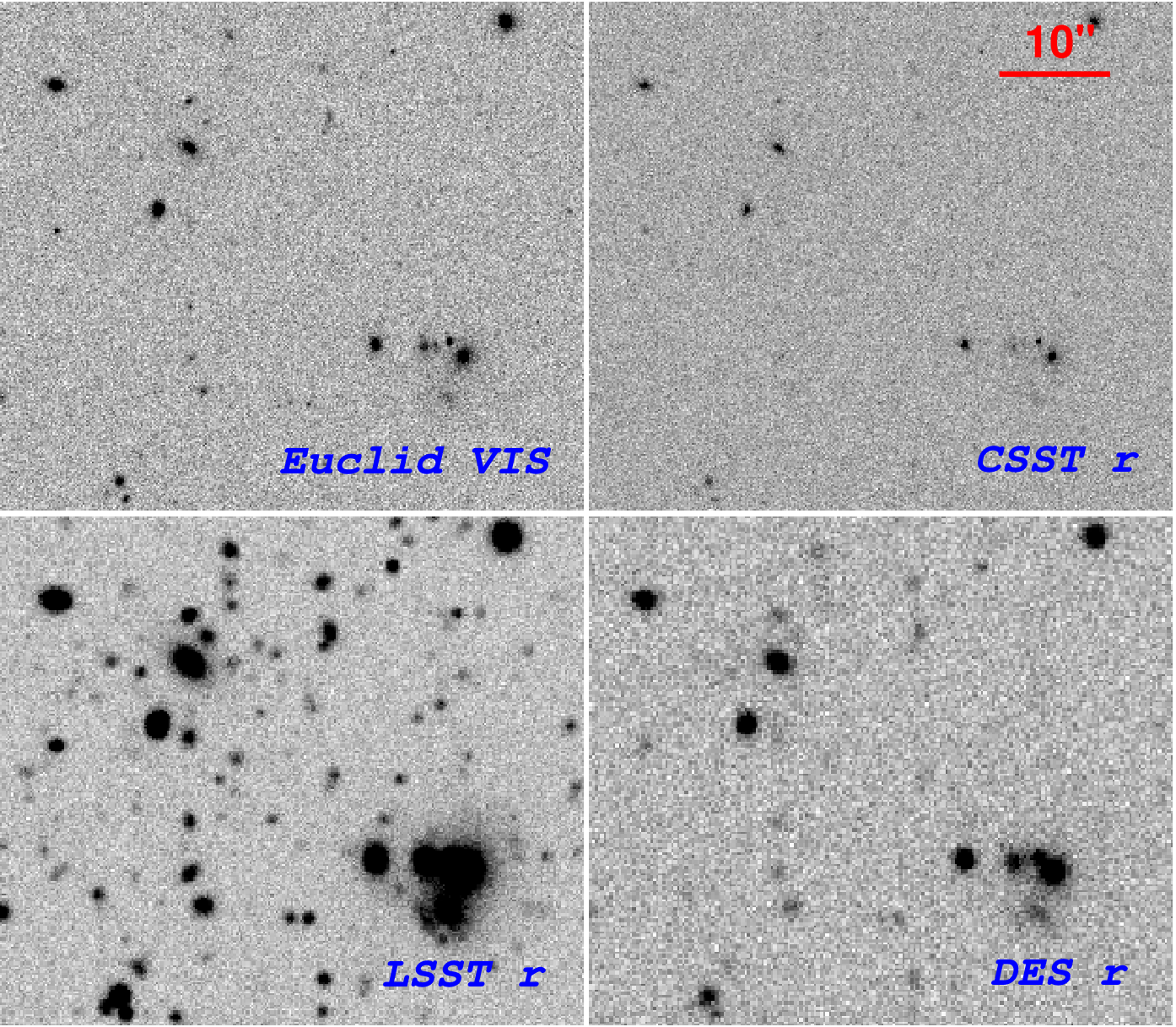
In total, we generate 22 sets of mock simulations corresponding to the 22 different bands, 7 for CSST, 4 for Euclid, 6 for LSST-like setup and 5 for DES-like setup. For each band, we have 20 sets of images with different noise realizations. Each image contains input galaxies covering an area of from HDUV GOODS-N. Fig. 2 shows examples of the simulated images for the Euclid VIS band, CSST band, LSST-like band, and DES-like band, respectively. Different survey characteristics are clearly seen. In particular, galaxies that are severely blended in ground-based observations can be better resolved in the two space-based surveys. In Fig. 3, we present the synthetic magnitude distributions (left) of the four surveys and the distribution of the intrinsic half-light radius (right) of the simulated galaxies from step (3).
With the mock images, we perform galaxy detection based on the Euclid VIS images employing SExtractor, and determine the 2-D elliptical aperture, known as the Kron radius (Kron 1980), in unit of arcsec for each galaxy. The parameters of the scaling factor and the minimum radius of a Kron ellipse in PHOT_AUTOPARAMS are set to be the default values of 2.5 and 3.5, respectively (Bertin & Arnouts 1996). The corresponding flux and magnitude enclosed within the elliptical aperture are defined as FLUX_AUTO and MAG_AUTO in SExtractor, respectively. Fig. 4 shows the SExtractor MAG_AUTO magnitude distribution of the detected galaxies in the solid histogram, while the dashed histogram corresponds to the distribution of galaxies with signal-to-noise (S/N) ratio above 10. The S/N is defined by the inverse of the magnitude error MAGERR_AUTO, that is S/N=1.0857/MAGERR_AUTO, which is a robust estimate here because the noise correlations do not presented in our simulated images (Newberry 1991; Bertin & Arnouts 1996). This figure shows that substantial incompleteness occurs for MAG_AUTO , approximately matching the designed limit for Euclid. From the 20 sets of Euclid VIS images, we obtain the average number of detected galaxies with MAG_AUTO being in the area of . The corresponding number density is , well in line with the Euclid specification. For comparison, we also perform parallel mock simulations using the COSMOS2015 catalogue as the input. The corresponding number density of Euclid VIS-detected galaxies is , much lower than that from our fiducial simulations based on the HDUV catalogue.
With the aperture determined from the VIS band, we perform forced photometry for each galaxy at the other bands. To ensure that the flux measurements from different bands contain the same fraction of the total flux, we perform PSF homogenization for all the bands. In our analyses, we assume the PSFs of different bands follow the two-dimensional circular Gaussian function, and thus the homogenization kernels are also Gaussian. Therefore for a certain band , the kernel size can be derived as , where is the PSF size of the band , and is the size of the target PSF (denoted as ). We then convolve the image of band with the Gaussian kernel to get the PSF homogenized image. This is performed through the convolve_fft function implemented in Astropy which is a community Python package for astronomy (Astropy Collaboration et al. 2013). To validate the quality of the convolution, we calculate the fractional error , where is the convolved PSF of band . It turns out that the fractional error is less than , indicating that the PSF homogenization is accurate. We note that for real observations, the PSF profiles can be more complicated. Thus the PSF homogenization needs to be done with sophisticated care (Hildebrandt et al. 2012; Skelton et al. 2014; Wright et al. 2019).
The specific PSF homogenizations for different data sets are as follows. For the CSST-only setup, the homogenization is based on the CSST -band PSF which has the largest size with . For the Euclid+DES-like setup, the DES-like -band PSF is used for homogenization. For the Euclid+LSST-like setup, we use the Euclid -band PSF for the homogenization. For the Euclid+CSST, because the large difference between the PSF sizes in the optical and NIR bands, we adopt a similar strategy as in Skelton et al. 2014 to perform homogeneous photometry. For the CSST and Euclid optical bands, we homogenize the images based on the CSST -band PSF, while for the Euclid NIR images, the homogenization is based on the -band PSF.
Because of the different treatment in the case of Euclid+CSST, we need to convert the measured aperture flux to the total flux of a galaxy. This is done using
| (1) |
where the scaling factor is the ratio of the total galaxy flux measured from the mock Euclid VIS images without PSF homogenization and the aperture flux of the corresponding PSF-homogenized Euclid VIS images, and is the aperture flux measured from the homogenized images of band . The FLUX_AUTO measured by SExtractor is used as the representation of the total flux of the galaxy. The aperture flux is measured by a circular aperture of radius , where is the semi-minor axis of the Kron ellipse which is used to measure the total flux . Since the Kron ellipses are different for different galaxies, the circular apertures are adaptive for different galaxies. We test this by applying different circular aperture settings, with where n ranges from 0.6 to 2.0 with a step of 0.2, and find that gives the best photo- results which are presented in Sect. 3.1.2. The photo- analyses with fixed apertures for all galaxies are also discussed in the next section. After the PSF homogenization the PSFs of the Euclid VIS images and the band images are expected to be identical. For the CSST and Euclid optical bands, is the aperture flux measured from the VIS-band images after being homogenized to the CSST -band PSF, while for the Euclid NIR bands, is measured from the VIS-band images after being homogenized to the -band PSF. For the other three setups, we also apply the conversion with the ratio being the same for all bands because a uniform homogenization is applied.
Differently from the original simulated images, it is noted that the PSF homogenization procedure can result in correlated noise between adjacent pixels. The flux errors measured by SExtractor are therefore underestimated since it does not consider the correlated noise (Leauthaud et al. 2007, e.g.). To estimate the flux errors with the presence of correlated noise, we follow the method as in Skelton et al. 2014 which is also adopted in many other studies (Gawiser et al. 2006; Liu et al. 2017, e.g.). For a specific aperture, the flux errors of galaxies in the PSF homogenized images of band can be estimated by
| (2) |
where is the pixel area in a given photometric aperture, is the standard deviation of the background noise, and is the correlation parameter to be determined. In the case of no correlation presented, , which is the formula used in SExtractor. On the other hand, if the adjacent pixels are perfectly correlated, . Generally, the value of is within the range of . To determine of band , we randomly generate a set of 2000 positions on the image that do not overlap with the detected objects. The fluxes are then measured for each position with different apertures. For a given aperture, a Gaussian function is applied to fit the distribution of the measured fluxes to derive the noise dispersion . It turns out that this dispersion gets larger with the increase of aperture size. We then use the power-law equation to fit the measured noise dispersion to find the best-fit value of . The derived values, typically ranging from 0.5 to 0.6 for different bands, are applied to Eq. (2) to calculate the flux errors. Finally, the flux errors are corrected to total in the same way as for the fluxes (see Eq. (1) above).
For photo- measurements with EAZY, we use the and corresponding as input, and denote the obtained photo- as . Because the purpose in this work is to compare the photo-s under different survey setups, we run EAZY with the same input configuration used to generate the SED templates. The configuration here ignores the template uncertainties in photo- estimates which is different from real cases that the optimizations of SED templates are necessary to improve the photo- quality as the real galaxy SEDs are not exactly the same as the input templates (Skelton et al. 2014).
3.1.2 Results
We show our photo- results in Fig. 5, where the upper left and right panels are for CSST-only and Euclid+CSST, and the lower left and right ones are for Euclid+LSST-like and Euclid+DES-like setups, respectively. Here the top plots show the results from data with a specific noise realization, while the bottom plots present the scatters from 20 sets of data with different noise realizations as described in the step (5) in Sect. 3.1.1. The vertical stripes seen in the bottom plots reflect the statistical fluctuations of different noise realizations. The photo- statistics for galaxies with VIS and are shown in Table 2. Here we use the conventional definitions with the bias given as
| (3) |
with , the normalized median absolute deviation of the residuals calculated by
| (4) |
and the outlier fraction being the fraction of galaxies with
| (5) |

Because of the deeper limiting magnitudes of the LSST-like survey after 10 years of observations, the Euclid+LSST-like case gives the best photo- accuracy with and considering galaxies with S/N in at least one of the LSST or bands. For the Euclid+DES-like setup, the numbers are and . For the combination of the two space missions, Euclid+CSST, we have , and . For the CSST-only setup, and . It is seen that for CSST, adding the Euclid NIR bands can improve the photo- measurements significantly, reducing the outlier fraction by more than a factor of .
In Fig. 6, we show , and at different redshifts . By comparing the results of Euclid+CSST with that of CSST-only, all the three photo- statistics are improved significantly for by including the NIR bands. As discussed extensively in the literature (Stabenau et al. 2008; Salvato et al. 2019; Newman & Gruen 2022, e.g.), the absence of ultraviolet or NIR data can result in difficulties in correctly identifying the Balmer and Lyman breaks in a galaxy SED. This will introduce large photo- errors. In our study, this problem is more significant for the photo- result of CSST-only setup because of the lack of NIR bands. This leads to larger , and at than the other cases as shown in Fig. 5 and Fig. 6.
We check the large outlier part in the upper left corner of the CSST-only case in Fig. 5, and also particularly analyse multiple cases in the region of where the CSST-only photo-s show relatively large positive biases . It is noted that for , the Balmer break and most of the emission lines except Ly are redshifted to the wavelength longer than band, and thus it is difficult to identify them accurately without NIR data. Furthermore, the true Lyman break is still in the blue side of NUV, and thus hard to be located correctly. The trend with relatively large photo- biases in this redshift range with optical data only is also shown in, for instance, Salvato et al. 2019 and Cao et al. 2018. In Fig. 7, a few examples are presented to illustrate clearly the reasons for the bias in the CSST-only case and the effects of NIR data. There the best-fit SEDs in the CSST-only (black) and Euclid+CSST (orange) cases, as well as the input SEDs (purple), are shown.
The top panel of Fig. 7 is for a case with the CSST-only photo- result drastically wrong by assigning a high to a low-redshift galaxy with . The middle panel shows a case with and the CSST-only . For these two cases, the SED behaviours are similar. With the CSST-only data, the Balmer break feature cannot be located well, and the best-fit redshifted SED gives rise to relatively higher NIR fluxes than the input SED. The Lyman break position (left black vertical line) is determined to be closer to CSST NUV than the true one, leading to higher than . Adding Euclid NIR data, the NIR part of the SED is better fitted and the Balmer break as well as the Lyman break positions (vertical orange lines) can be correctly identified. As a result, the best-fit SED and consequently the photo- from Euclid+CSST are in better agreement with the input ones. The bottom panel of Fig. 7 shows another case with where the CSST-only best-fit SED has about the correct shape in NIR comparing to the input one, but the Lyman break position is determined to be at a somewhat longer wavelength, and thus a higher . In this case, the inclusion of Euclid NIR adds weights to adjust the overall SED including the two break positions, delivering a better photo- of .
For the combinations of Euclid with LSST-like, CSST, and DES-like setups, respectively, over the entire redshift range, both and are the largest for the case of Euclid+DES-like. It should be noted that in our analyses, the same set of templates are used in generating the input fluxes in different bands and in the photo- fitting. Thus, the overall small bias here is largely due to photometric errors. In real situations, if the true SEDs of some galaxies are not included in the templates, their photo- bias from template fitting can be significantly larger than the numbers shown here.
| Combination | bias | ||
|---|---|---|---|
| CSST-only | 0.0043 | 0.048 | 8.45% |
| Euclid+CSST | 0.0051 | 0.039 | 2.39% |
| Euclid+LSST-like | 0.0019 | 0.018 | 0.83% |
| Euclid+DES-like | 0.0057 | 0.054 | 12.87% |
We emphasize that our purpose here is to compare different data combinations, and thus the relative differences in photo- accuracy between different cases are more meaningful to us. While the absolute photo- accuracy can be sensitive to the adopted methods and codes (Hildebrandt et al. 2010; Euclid Collaboration et al. 2020b; Zhou et al. 2021), the relative accuracy should depend mainly on the data used. We therefore only use the EAZY template fitting code to do the photo- analyses here and leave the thorough investigations on photo- measurement methods to future studies.
It should also be noted that in our analyses, we do not consider the effect of AGNs. Studies have shown that galaxies hosting AGNs generally have worse photo- quality (Salvato et al. 2019, e.g.). At high redshifts, faint AGNs cannot be easily identified (Małek et al. 2013; Golob et al. 2021, e.g.). Thus their flux contaminations to their host galaxies can lead to errors in the photo- estimation. MacDonald & Bernstein 2010 studied the photo- bias induced by AGN contamination, and concluded that this bias can potentially corrupt the derived cosmological parameters, especially for future WL surveys reaching deeper limiting magnitudes. As described in Sect. 3.1, Euclid selects its shear sample with one of the criteria by requiring that the galaxies therein should not be flagged as AGNs (Euclid Collaboration et al. 2020b). This can mitigate the AGN-induced photo- bias to some extent. However, for unidentified AGNs, their effects on photo- measurements need to be addressed in future studies.
In addition, we also do not perform careful deblending for ground-based images. On the other hand, to suppress the blending effects on ground-based photometry, we employ the positions and apertures measured from high-resolution Euclid VIS simulated data for flux measurements on LSST-like or DES-like images. A potential problem for such an approach is that for some galaxies, the Euclid VIS apertures can be too small for the two ground-based-like images, and thus their measured are sub-optimal.
To see the impact of photometric apertures, we measure galaxy fluxes using different apertures taken to be , where is a factor and is the FWHM of the PSF after homogenization. Specifically, and for the case of Euclid+LSST-like, Euclid+DES-like, Euclid+CSST, and CSST-only, respectively. As explained previously, for Euclid+CSST, high-resolution images from CSST and the Euclid VIS-band as well as the PSF homogenized Euclid -band images are used in the photo- analyses. Thus, we take here, which is the FWHM of the Euclid -band PSF used in the homogenization. The aperture flux in each band is scaled to the total flux with Eq. (1).
We calculate the variations with the change of for LSST-like galaxies. Different from point sources, galaxies have various intrinsic sizes, and the dependence of their on the aperture size can be different. We therefore bin galaxies based on their intrinsic size defined in the simulation step (3), and calculate the average within a bin. We further note that galaxies of similar size can have a range of intrinsic luminosity. To clearly illustrate the aperture effect on , for each LSST-like galaxy, we calculate the ratio of the signal-to-noise ratio measured within an aperture diameter to that measured within the Euclid VIS aperture, that is . The results are shown in Fig. 8, where the lines are the average and the shaded regions are the corresponding dispersion. It is seen that for galaxies with , the optimal aperture is about where . In other words, for these relatively large galaxies, using Euclid VIS aperture is a good choice. For smaller galaxies, reaches the maximum at and –1.4, that is Euclid VIS apertures are sub-optimal for LSST-like images homogenized to a PSF with FWHM .
To illustrate the impact of the aperture on the photo-, we show the dependence of and on the aperture parameter in Fig. 9 for different cases. There we also show the results of Euclid+LSST-like setup, using LSST-like data of different depths, which correspond to different years of accumulation. We see that for both Euclid+LSST-like and Euclid+DES-like, and are nearly flat for , and their values are very close to the ones shown in Table 2 using Euclid VIS apertures. This seems to indicate that although Euclid VIS apertures are not optimal for small galaxies, their effects on photo- are not very significant. Increasing the aperture factors from to , the outlier rate increases considerably, for the case of Euclid+LSST-like by factors of to for LSST-like Year01 to Year10. The also increases by about a factor of . These trends are largely attributed to the light blending of nearby galaxies plus the reduced at large apertures as shown in Fig. 8. Similar behaviours are seen for the results of the Euclid+DES-like case. For Euclid+CSST, the changes of and are much flatter over the whole range from to . This is because the high resolution optical images from CSST and Euclid VIS are much more compact than those of LSST-like or DES-like setups, and therefore the light blending effect is much weaker even with similar photometric apertures. In terms of the outlier rate , Euclid+CSST can reach approximately the same accuracy as that of Euclid+LSST-like YEAR02 data when using an aperture diameter less than .
We need to point out that accurate multi-band photometric measurements are challenging and should be carefully investigated based on the specific data characteristics. Our analyses here, either using Euclid VIS apertures in our fiducial analyses or the tests using different fixed apertures, are somewhat sub-optimal in the sense that we do not perform detailed aperture optimisation band by band and galaxy by galaxy. With more sophisticated optimisations (Kuijken 2008; Kuijken et al. 2015; Wright et al. 2016; Bosch et al. 2018; Huang et al. 2018; Sevilla-Noarbe et al. 2021, e.g.), the photo- statistics may be further improved compared to the results shown here. Although we do not expect qualitative changes of our conclusions, quantitative studies and comparisons with different photometric measurements are desired in future investigations.
We also emphasize again that we do not perform careful deblending for ground-based-like images. The performance of photo- in the case of Euclid+LSST-like (DES-like) can be improved by employing sophisticated approaches for accurate photometric measurement. On the other hand, for the data combination of Euclid and CSST, the blending in optical bands is minimal, and thus the photometric measurements can be relatively straightforward.
3.2 Blended galaxies
As we discussed in the previous section, with the increase of observational depth blended galaxies for ground-based observations are becoming increasingly problematic for accurate photometry. For HSC, the estimated fraction of blended galaxies is about 58% (Bosch et al. 2018). For LSST, the fraction will be even higher. To achieve high-precision cosmological results from galaxy imaging surveys, sophisticated deblending algorithms are critically needed.
In SExtractor the deblending is done on single-band images by using a tree structure to find sub-objects with the intensity above a certain fraction of the total intensity of the composite object. The intensity of overlapping pixels are assigned to different sub-objects according to bivariate Gaussian fits to the sub-objects (Bertin & Arnouts 1996). In recent years, more advanced methodologies have been developed. For example, MuSCADeT (Joseph et al. 2016) and SCARLET (Melchior et al. 2018) utilize multi-band pixel information for deblending, and thus galaxy SEDs are taken into account. However, similarly to SExtractor, these methods still make certain assumptions about galaxy properties. Another line of study is to use machine learning for deblending, which on the one hand can avoid overly simplifying assumptions about galaxies. On the other hand, appropriate training sets are crucial for machine learning (Reiman & Göhre 2019; Arcelin et al. 2021; Farrens et al. 2022).
In this regard, space observations with high resolution are clearly advantageous in reducing the fraction of blended galaxy images, and thus simplifying the photometric measurements. To explore the advantages of utilizing data from the two space missions to control blending, we create a set of dedicated simulations, which differ from the simulations presented in Sect. 3.1.1. We start here from HST/CANDELS GOODS-N images of F606W and F814W (Giavalisco et al. 2004; Grogin et al. 2011; Koekemoer et al. 2011). The effective area is about 158 arcmin2. These image stacks have been created using 006 pixels. We synthesize Euclid VIS and CSST -band images from them. For comparison, we also generate LSST -band images.
Specifically, to generate Euclid VIS images, we first combine CANDELS F606W and F814W pixel data using linear interpolation as follows,
| (6) |
where nm, nm, and nm are the central wavelengths of F606W, F814W, and the Euclid VIS band, respectively. The zero-points related to the rescaling of F606W and F814W are and . We take and thus with zpi the zero points for the two CANDELS bands. The corresponding widths of the three bands are , and . For CSST - and LSST -bands, we simply use the CANDELS F606W images, ignoring the slight band difference.
We then convolve these idealized images, labeled as , with the corresponding PSF, and resample them according to the pixel scales of Euclid VIS, CSST - and LSST -bands, respectively, with the parameters listed in Table 1. We denote these PSF- and pixel-scale-matched images as . In the last step, we add Gaussian noises to according to the three survey depths to generate the final images. In this simulation setting, we assume that the HST CANDELS images are ideal without considering their own PSF and noise. For the purpose of analysing blending effects of different surveys, this simplification should not affect the results significantly.
In Fig. 10, we show examples of the simulated images, where the left panels are images and the right ones are the corresponding images. It is seen clearly that both Euclid VIS and CSST band observations can resolve galaxies similarly to the HST CANDELS data. For ground-based LSST-like data, however, the blending effect is much more severe.

Fig. 11 shows quantitatively the blending statistics. Here we perform source detection using SExtractor on images for the three cases separately. The dashed lines show the results with the blended galaxies defined using the SExtractor FLAGS=1 and 2, and the values containing the contributions from these two flags. Here, FLAGS=1 indicates a likely contamination of the aperture photometry by neighbouring sources, and FLAGS=2 shows that the object has been deblended (Bertin & Arnouts 1996). The solid lines present the blending statistics defined as the occurrence of overlapping between 2.5 times expanded Kron ellipses with neighbouring galaxies. The upper and lower panels show the dependence of the cumulative number density of blended galaxies on the magnitude, and the corresponding fractions. Note that the horizontal axis shows the magnitude of the galaxies we are concerned with. To judge if they are blended, however, we are not limited to this magnitude, but use all detected galaxies instead. We can see that for LSST-like images, the number density of blended galaxies can reach about 30–50 arcmin-2 at depending on the definition of blending. For Euclid and CSST, the corresponding number density is about 5 arcmin-2. The blended fraction is computed as the ratio of the numbers shown in the upper panel and the corresponding total detected number densities of galaxies at the same magnitude cut. It is at for both Euclid and CSST, while for the LSST-like data, it is in the range of to .
In the above analyses, the source detection and the blending identification are done independently for each of the three sets of mock survey simulations. There can be cases that two or more close-by galaxies in a high-resolution image are identified as a single galaxy in a low-resolution LSST-like image. We refer to these as total blends, and they cannot be correctly counted in Fig. 11. To calculate the fraction of total blends for the LSST-like case, we perform analyses by matching the Euclid VIS detected galaxies with those detected from LSST-like images. Specifically, we first perform a double-match with a given matching radius between Euclid VIS and LSST-like galaxies, and then remove those matched ones from the Euclid VIS galaxy catalogue. For the remaining galaxies, we perform a second double-match with the full LSST-like galaxy catalogue. If two Euclid galaxies are matched to a single LSST-like galaxy, we regard the latter as a total blend. In Fig. 12, the bottom panels show an example of total blends with the left and right panels being Euclid VIS and LSST-like -band images, respectively. The top panel shows the fraction of total blends in the LSST-like case with respect to the matching radius . For , the size of the LSST-like PSF FWHM, the fraction is about , and it increases to for .

To study the impacts of blending on photometry, we first measure the MAG_AUTO magnitude of each detected object using SExtractor on images of the LSST-like band and the CSST band, respectively. They are at high resolution without noise. We then carry out the photometry measurements on the corresponding images, which are PSF-convolved and pixel scale-matched images but contain no noise. The comparison of these two sets of photometry can reveal cleanly the blending effects. For the Euclid VIS band, the results are similar to those of CSST because of the similar PSF, and thus they are not shown here. The top left panel of Fig. 13 shows the scatter plot of the two sets of measurements, where the horizontal axis shows the magnitude and the vertical axis is the difference of the magnitudes measured in the and images. The lines are the median bias of the corresponding cases. It is seen clearly that in the LSST-like case, the severe blending effects lead to magnitude estimates that are significantly biased low, that is brighter, with the median bias at , , and being 0.135, 0.175 and 0.215 , respectively. For CSST, the corresponding bias is about 0.038, 0.042, and 0.052 mag. The distributions of the are shown in the top right.
From the distributions, it is noted that the is systematically positive, meaning that the MAG_AUTO magnitudes measured in images are systematically brighter than that of images. Our tests show that this is attributed to the larger Kron ellipses (in unit of arcsec) used in images than that of in images due to both the PSF effect and the pixel downsampling from to . Firstly, the PSF smoothing operation tends to smear the surface brightness distributions of the galaxies and reduce the random background noise. Secondly, the downsampling operation of the pixel scale from to images can also reduce the random background noise and thus increase the S/N of the galaxies in . Both result in a smaller MAG_AUTO measured from and thus the distributions shown in the top panel of Fig. 13 being peaked at a positive . On the other hand, it is the blending effects that lead to a significantly extended tail at the positive side of the distribution, especially in the case of LSST-like. The bottom panels of Fig. 13 present three examples of galaxy images. In each of these panels, the left sub-panels are the CSST (top) and LSST-like (bottom) images while the right sub-panels show the corresponding images. They demonstrate how the blending effect impacts the ground-based photometry at different levels. Here again, the larger Kron ellipses due to PSF smoothing and image downsampling can be seen on the images. Note that SExtractor provides a deblending procedure. However, this is clearly not good enough. More sophisticated deblending techniques are needed. On the other hand, for the two space missions, the blending effect is much lower, and the photometric measurements can be significantly simplified.

The photometry results shown in Fig. 13 correspond to SExtractor MAG_AUTO magnitudes, which are intended to measure the total magnitude of galaxies directly from images. In other words, if considering joint analyses of different surveys, such measurements can be used for data combinations at the catalogue level. Because of the PSF smoothing and image downsampling, the aperture used to compute MAG_AUTO is significantly larger in the case of LSST-like simulations compared to the simulated space-based data, causing severe blending effects and biases in the photometry. Using space observations as priors, the photometry can be improved significantly (Chary et al. 2020; Melchior et al. 2018, e.g.). This demands that the data combination must be done at the pixel level. In fact, in our photo- analyses in Sect. 3.1, we adopt the Euclid VIS detection to provide a position prior, and the photometric aperture for a galaxy is also from Euclid VIS. We then apply them to other cases considering the scaling relation of Eq. (1). We perform such measurements here to and images of different cases, and the results are presented in Fig. 14. By comparing with the results shown in Fig. 13, we can see that the bias in the LSST-like case is indeed reduced significantly. For CSST, the results are nearly the same. This reveals to us that for the two space missions, the data combination at the catalogue level may be sufficient. By including ground-based data, however, careful treatments at the pixel level are necessary.
For the total blends in the LSST-like case shown in Fig. 12, we calculate the flux ratio of the blended galaxies from high-resolution Euclid VIS images. The results are presented in Fig. 15, where the left panel shows the flux ratio vs. the LSST-like -band magnitude of the total blends. Different sub-panels are for the total blends using different matching radius , and the dashed lines are the corresponding medians. The distributions of the flux ratio for the cases shown in the left are presented in the right panel where they are all divided by the number of total blends in the case of . Thus the areas under the curves reflect the relative probabilities with respect to the case of . The median flux ratio increases with the decrease of the matching radius, but the probability of total blends with smaller matching radius is lower. For , the median flux ratio is , and at the LSST-like , and , respectively.
To show the blending effects on photo-s, in Fig. 16, we re-plot the results of Euclid+LSST-like Year10 data and Euclid+CSST with different photometric apertures specified in Sect. 3.1. In addition, we also show the results for the Euclid+LSST-like case but discarding the galaxies with neighbours within . It is seen that by removing those potential blended galaxies, the outlier rate is reduced significantly for the aperture size larger than . This shows clearly the blending effect on the photo- measurements for ground-based observations, and careful deblending, which is not studied here, is needed for relatively large aperture sizes. For Euclid+CSST, because of the high-resolution images in optical bands, the effect of the aperture size resulting from the blending on photo- accuracy is much weaker, showing the advantage of the space-space data combination of Euclid and CSST with similarly high resolutions in optical bands.
3.3 PSF chromaticity
The wide Euclid VIS band is designed to increase the signal-to-noise ratio of galaxies for accurate shear measurements. However, this leads to a significant chromaticity of the PSF. The effective PSF depends on the SED of each object. It can differ systematically for stars and galaxies. This can lead to significant biases in the shear measurement if not carefully accounted for (Cypriano et al. 2010; Eriksen & Hoekstra 2018; Meyers & Burchat 2015; Carlsten et al. 2018, e.g.).
CSST has seven bands from NUV to , and can provide valuable SED information for stars and galaxies. Such information can be used for Euclid to obtain accurate PSF measurements from stars. The PSF interpolation to galaxies can also be improved by including galaxy SEDs at high angular resolution, and thus reducing the PSF chromaticity bias in shear measurements. In addition, CSST is equipped with slitless spectrometers for galaxy redshift surveys. They cover the wavelength range from 255 nm to 1000 nm, divided into the three bands GU, GV, and GI. The spectral resolution is . For the wide survey, the cumulative magnitude limit within each of the three bands is about (5 for point source). For the deep survey, it is one magnitude deeper. The spectral data from CSST can then provide high-resolution stellar SEDs, which can further improve the Euclid PSF construction compared to the use of photometry-based SED estimates.
For extended galaxies, besides the PSF chromaticity bias described above, there is also a colour gradient (CG) bias in the shear measurement resulting from SED differences within a galaxy. The amplitude of the CG bias depends on several factors: the SED of the galaxy, the relative size of the galaxy compared to the PSF, and the width of the filter. The wide bandpass of the Euclid VIS filter can lead to a non-negligible CG bias. It has been demonstrated that the Euclid VIS CG bias can be calibrated using high spatial resolution data from two narrower bands covering the VIS bandpass (Semboloni et al. 2013; Er et al. 2018). The analyses show that for each type of galaxies based on, e.g. galaxy size, bulge-to-total flux ratio and SED, their average multiplicative CG bias can be calibrated down to the 0.1% level using 50 images with in the two narrower bands (Er et al. 2018).
CSST has a similar spatial resolution and a smaller pixel scale of than that of Euclid VIS. The bands from CSST can thus provide narrower-band data for Euclid CG bias calibration. In order to see if CSST surveys can provide a sufficient number of high- galaxy images, we calculate the statistics of the of CSST galaxies from our mock CSST simulations.
As noted in Sect. 4.1, the HDUV catalogue has a relatively small size. Although we generate 20 sets of mock images by adding different realizations of noise, for each galaxy, its input parameters, including position, redshift, intrinsic size and are the same in all the 20 sets. Thus the statistics in terms of these parameters concerned in the CG bias calibration are limited by the input HDUV catalogue. In comparison, the COSMOS2015 catalogue covers a much larger sky area and thus contains many more galaxies (Laigle et al. 2016). We therefore use the parallel CSST mock simulations based on the COSMOS2015 catalogue for the statistical analyses here.
Specifically, we consider a portion of the COSMOS field covering an area of centered at (RA, DEC) = (). The selected field provides a large enough galaxy sample while being less affected by saturated star masks. Meanwhile, to avoid bad photometric measurements, we select galaxies by constraining the parameter FLAGS in band to be smaller than 3, meaning that galaxies suffering from the impact of saturation or truncation are excluded, but those with close neighbours are kept. The redshift of a galaxy is taken to be the median value of its photo- likelihood distribution (PHOTOZ==ZPDF) given in the COSMOS2015 catalogue. To acquire the size and orientation parameters of these galaxies, we match them with the HST/ACS F814W-band catalogue (Leauthaud et al. 2007) using a matching radius of . Finally, we have 99 264 galaxies as input for the image simulations. We follow the simulation steps described in Sect. 3.1.1 to generate mock multi-band images for the CSST wide survey and also for the CSST deep survey which is about one magnitude deeper than the wide one. In accord with the studies in Er et al. 2018, we consider calibrations using two narrower bands. We therefore stack the images of bands and bands separately to build the calibration data sets.
In Fig. 17, we show the distributions of galaxies from CSST wide (top) and deep (bottom) simulations. Here we only consider galaxies with Euclid VIS . For comparison, we scale the galaxy numbers here to a sky area of , the planned coverage of the CSST deep survey. The corresponding number of galaxies with is and for the wide and deep cases, respectively. We further consider galaxies with different properties. It is known that the bulge and disk components of galaxies typically have different SEDs. Thus galaxies with different can have different CG biases, and need to be calibrated separately. We therefore bin galaxies based on and calculate the for galaxies in each bin. Fig. 18 shows the number distribution of galaxies with with respect to from CSST deep simulations. It is noted that the absence of galaxies in the range is attributed to the input distribution as described in Sect. 3.1.1. We can see that the CSST deep survey can provide sufficient numbers of galaxies in nearly all the bins for Euclid to calibrate the CG bias.
We further analyse the feasibility of calibration in finer grids of galaxy parameters. In Fig. 19, the top panel shows the number distribution of galaxies with expected from the full CSST deep survey in 2-D grids of vs. redshift . Here the bin sizes are for , and () for at (). The bottom panel is for the number distribution in vs. the intrinsic size of galaxies defined in Sect. 4.1 for galaxies in the redshift range of . One can see that the deep survey shall be able to provide a calibration sample up to . At , we can perform analyses for different types of galaxies separately, leading to more accurate calibrations for the CG bias for galaxies with different and size.
As we discussed, because of the ground-based source detection, the COSMOS2015 catalogue has a lower number density of galaxies than that of the HDUV catalogue with the source detection from the high-resolution HST images. Thus the statistics shown here are conservative. We expect that the CSST deep survey can provide a larger number of high- galaxies than that seen in Fig. 17 to Fig. 19 for Euclid to calibrate the CG bias.
Besides CG bias calibration for different samples of galaxies, it may even be possible to correct for the bias for individual galaxies with CSST high multi-band data. We leave this for future studies.


4 Further science
Apart from WL analyses, the complementarity of the data from Euclid and CSST can benefit many more areas of research. Here we briefly mention a few topics that are outside of WL but relate to cosmology. They especially make use of the multi-band imaging data and the resulting photometric measurements.
The high resolution and large sky coverage of the two surveys allow us to find strong-lensing systems. Their identification requires deep-learning-based machinery (Metcalf et al. 2019, e.g.). The colour information from the joint multi-band imaging data can improve the efficiency and accuracy of the strong-lensing system detection considerably (Petrillo et al. 2019; Pearson et al. 2019, e.g.). Furthermore, Euclid+CSST can provide accurate photo-s for both lenses and sources, and thus additional information on the geometrical distances of lens systems. This can tighten the lens modelling significantly. One of the major science cases of strong lensing in both CSST and Euclid is to detect small perturbations to Einstein rings/giant arcs, which can put constraints on the nature of dark matter (Li et al. 2016; Li et al. 2017, e.g.). This requires very accurate modelling of the lens mass distribution. Data from independent surveys can provide unique discriminating tests of the model accuracy. In addition, because of the wavelength-dependence of the light distribution for a source galaxy, its lensed image positions in the optical and NIR can be different. Therefore, the joint lensing analyses from CSST optical and Euclid NIR observations provide more sample points to constrain the lens potential, helping to break degeneracies in the lens modelling.
The photo- measurements from Euclid+CSST can also improve the detection of clusters of galaxies. In particular, the NIR bands from Euclid can lead to more efficient identifications of high-redshift clusters comparing to that with CSST 7 bands only (Wen & Han 2021). The improved photo- accuracy is also important to allow us to probe tomographic galaxy clustering using photometric galaxy samples, which typically have a much larger number of galaxies extending to higher redshifts than that of spectroscopic galaxy samples.
Additionally, the data from NUV to from Euclid+CSST will form a great data pool for legacy studies, such as galaxy formation and evolution, near-field cosmology, etc.. As an example, the high-resolution multi-band data from the two space missions will allow robust SED modeling, with, e.g. CIGALE (Boquien et al. 2019; Yang et al. 2020), to derive the physical properties, such as the stellar mass, star formation rate for a large sample of galaxies. Carefully decomposing light from AGNs and host galaxies can also provide information about the AGN luminosity function to the faint end. Combining with the spectroscopic data from the two surveys, it is expected that the synergy will give new insights into the formation and evolution of galaxies and AGNs as well as the large-scale structures of the Universe. Because both projects have different working groups investigating on different subjects, detailed explorations of the synergy in areas other than WL cosmology is beyond the scope of our studies here.
5 Discussion and conclusions
The high-quality multi-band data from upcoming large surveys will allow us to probe the Universe with an unprecedented precision. How to efficiently utilize data from different surveys to enhance the science gains is becoming an increasingly important topic.
In this study, we focus on the two space missions, Euclid and CSST, and investigate their potential synergies emphasizing the aspects related to the weak lensing studies. While having a similar high spatial resolution and largely overlapping sky coverage, the two missions cover different wavebands. Their combination can produce multi-band data from NUV to for over a billion galaxies. We analyse the photo- performance from Euclid+CSST. For galaxies with Euclid VIS and , the dispersion is , and the outlier fraction is . The precision is comparable to that from the combination of the Euclid+LSST-like 2 – 3 year data. Because of the similar sky coverage, the utilization of the data from the two space missions can be done in a uniform way, and thus the systematic errors in the data processing can be well controlled. This is advantageous over the combination of Euclid with several different ground-based surveys with different performance characteristics. Compared with the photo- results from CSST seven bands only, the inclusion of the Euclid NIR bands leads to a significant reduction of the outlier fraction from to .
We also carry out simulations to investigate the image blending effects. For Euclid and CSST, because of their high resolutions, the blending effects are minimal, and thus a catalogue-level data combination from the two space missions is feasible. For combining with ground-based data, however, pixel-level analyses with careful deblending are necessary. While there are still blended galaxies for the simulated space-based observations, their fraction is much lower compared to ground-based observations. Their deblending can be done efficiently by employing multi-band pixel data from CSST and Euclid. This will be investigated in future studies.
Analyses of Euclid VIS data are significantly affected by the PSF chromaticity. Accordingly, the addition of multi-band imaging and slitless spectroscopic observations from CSST can improve the Euclid VIS PSF modelling, and provide calibrations for chromaticity bias and the CG bias in shear measurements. Our studies show that the CSST 400 deg2 deep multi-band photometric survey can provide a large sample of galaxies with high . Therefore the multiplicative CG bias can be well calibrated to the level of for Euclid galaxies with different , and at different redshifts up to . On the other hand, the NIR data from Euclid can be valuable for CSST for a better star-galaxy separation and thus to improve the precision of the PSF construction.
The studies shown here assume the full availability of the data. The two missions have however different schedules. Euclid is expected to be launched in early 2023, and CSST targets late 2023 or early 2024 for launching. It is also noted that for CSST, different filters are distributed across the focal plane. Hence, the survey strategy will impact how quickly observations in all filters can be completed for a certain patch of the sky. With Euclid in orbit first, it might be worth thinking of a coordinated survey strategy for CSST, so that the synergies of the two missions can be realized in the early years of the surveys. The joint studies can benefit many more areas of astrophysical research beyond the WL analyses presented here. Given the great potential, possible survey coordination between the two missions, both for the wide and deep survey components, deserves further careful investigation.
Acknowledgements.
This research was initiated under the support of the ISSI/ISSI-BJ International Team Programs. All the Chinese coauthors acknowledge the science research grants from the China Manned Space Project with Nos.CMS-CSST-2021-A01 and CMS-CSST-2021-B01. The Bonn group acknowledges support from the German Federal Ministry for Economic Affairs and Energy (BMWi) provided through DLR under projects 50QE1103 and 50QE2002, as well as funding provided by the European Union’s Horizon 2020 research and innovation programme under grant agreement No. 776247. DZL acknowledges the support from NSFC under the grant of 12103043. ZHF is supported in part by NSFC under 11933002, U1931210 and 11333001. RL acknowledges the NSFC grands of 11988101,11773032 and 12022306, and the support from K.C.Wong Education Foundation, CAS Project for Young Scientists in Basic Research (No. YSBR-062). DS is a member of the International Max Planck Research School (IMPRS) for Astronomy and Astrophysics at the Universities of Bonn and Cologne. HYS acknowledges the supports from NSFC under 11973070, the Shanghai Committee of Science and Technology under the grant No.19ZR1466600 and Key Research Program of Frontier Sciences, CAS, Grant No. ZDBS-LY-7013. YST acknowledges the financial support from the Australian Research Council through DECRA Fellowship DE220101520. LPF acknowledges the supports from NSFC grants 11933002, and the Dawn Program 19SG41 & the Innovation Program 2019-01-07-00-02-E00032 of SMEC. HHi is supported by a Heisenberg grant of the Deutsche Forschungsgemeinschaft (Hi 1495/5-1). HHi and AHW acknowledge support by the ERC (Consolidator Grant No. 770935). XKL acknowledges the supports from NSFC of China under grant no. 11803028 and no. 12173033, and YNU grant no. C176220100008. The COSMOS2015 sample is based on data products from observations made with ESO Telescopes at the La Silla Paranal Observatory under ESO programme ID 179.A-2005 and on data products produced by TERAPIX and the Cambridge Astronomy Survey Unit on behalf of the UltraVISTA consortium. The employed CANDELS images are based on observations taken by the CANDELS Multi-Cycle Treasury Program with the NASA/ESA HST, which is operated by the Association of Universities for Research in Astronomy, Inc., under NASA contract NAS5-26555.References
- Abbott et al. (2021) Abbott, T. M. C., Adamów, M., Aguena, M., et al. 2021, ApJS, 255, 20
- Abbott et al. (2022) Abbott, T. M. C., Aguena, M., Alarcon, A., et al. 2022, Phys. Rev. D, 105, 023520
- Aihara et al. (2018) Aihara, H., Arimoto, N., Armstrong, R., et al. 2018, PASJ, 70, S4
- Albrecht et al. (2006) Albrecht, A., Bernstein, G., Cahn, R., et al. 2006, astro-ph/0609591
- Arcelin et al. (2021) Arcelin, B., Doux, C., Aubourg, E., Roucelle, C., & LSST Dark Energy Science Collaboration. 2021, MNRAS, 500, 531
- Astropy Collaboration et al. (2013) Astropy Collaboration, Robitaille, T. P., Tollerud, E. J., et al. 2013, A&A, 558, A33
- Bartelmann & Schneider (2001) Bartelmann, M. & Schneider, P. 2001, Phys. Rept., 340, 291
- Bertin & Arnouts (1996) Bertin, E. & Arnouts, S. 1996, A&A Suppl., 117, 393
- Boquien et al. (2019) Boquien, M., Burgarella, D., Roehlly, Y., et al. 2019, A&A, 622, A103
- Bosch et al. (2018) Bosch, J., Armstrong, R., Bickerton, S., et al. 2018, PASJ, 70, S5
- Brammer et al. (2008) Brammer, G. B., van Dokkum, P. G., & Coppi, P. 2008, ApJ, 686, 1503
- Cao et al. (2018) Cao, Y., Gong, Y., Meng, X.-M., et al. 2018, MNRAS, 480, 2178
- Carlsten et al. (2018) Carlsten, S. G., Strauss, M. A., Lupton, R. H., Meyers, J. E., & Miyazaki, S. 2018, MNRAS, 479, 1491
- Casertano et al. (2000) Casertano, S., de Mello, D., Dickinson, M., et al. 2000, AJ, 120, 2747
- Chary et al. (2020) Chary, R., Helou, G., Brammer, G., et al. 2020, arXiv:2008.10663
- Cypriano et al. (2010) Cypriano, E. S., Amara, A., Voigt, L. M., et al. 2010, MNRAS, 405, 494
- Dark Energy Survey Collaboration et al. (2016) Dark Energy Survey Collaboration, Abbott, T., Abdalla, F., et al. 2016, MNRAS, 460, 1270
- Eifler et al. (2021) Eifler, T., Simet, M., Krause, E., et al. 2021, MNRAS, 507, 1514
- Er et al. (2018) Er, X., Hoekstra, H., Schrabback, T., et al. 2018, MNRAS, 476, 5645
- Eriksen & Hoekstra (2018) Eriksen, M. & Hoekstra, H. 2018, MNRAS, 477, 3433
- Euclid Collaboration et al. (2020a) Euclid Collaboration, Blanchard, A., Camera, S., et al. 2020a, A&A, 642, A191
- Euclid Collaboration et al. (2020b) Euclid Collaboration, Desprez, G., Paltani, S., et al. 2020b, A&A, 644, A31
- Euclid Collaboration et al. (2022) Euclid Collaboration, Scaramella, R., Amiaux, J., et al. 2022, A&A, 662, A112
- Fan (2018) Fan, Z. 2018, 42nd COSPAR Scientific Assembly. Held 14-22 July 2018, in Pasadena, California, USA, Abstract id. E1.16
- Farrens et al. (2022) Farrens, S., Lacan, A., Guinot, A., & Vitorelli, A. Z. 2022, A&A, 657, A98
- Fu & Fan (2014) Fu, L. & Fan, Z. 2014, RAA, 14, 1061
- Fu et al. (2008) Fu, L., Semboloni, E., Hoekstra, H., et al. 2008, A&A, 479, 9
- Gawiser et al. (2006) Gawiser, E., van Dokkum, P. G., Herrera, D., et al. 2006, ApJS, 162, 1
- Giavalisco et al. (2004) Giavalisco, M., Ferguson, H., Koekemoer, A., et al. 2004, ApJ, 600, L93
- Golob et al. (2021) Golob, A., Sawicki, M., Goulding, A. D., & Coupon, J. 2021, MNRAS, 503, 4136
- Gong et al. (2019) Gong, Y., Liu, X., Cao, Y., et al. 2019, ApJ, 883, 203
- Grogin et al. (2011) Grogin, N., Kocevski, D., Faber, S., et al. 2011, ApJS, 197, 35
- Guinot et al. (2022) Guinot, A., Kilbinger, M., Farrens, S., et al. 2022, A&A, 666, A162
- Guo et al. (2013) Guo, Y., Ferguson, H. C., Giavalisco, M., et al. 2013, ApJS, 207, 24
- Guy et al. (2022) Guy, L. P., Cuillandre, J.-C., Bachelet, E., et al. 2022, in Zenodo id. 5836022, Vol. 58, 5836022
- Heymans et al. (2021) Heymans, C., Tröster, T., Asgari, M., et al. 2021, A&A, 646, A140
- Heymans et al. (2012) Heymans, C., van Waerbeke, L., Miller, L., et al. 2012, MNRAS, 427, 146
- Hikage et al. (2019) Hikage, C., Oguri, M., Hamana, T., et al. 2019, PASJ, 71, 43
- Hildebrandt et al. (2010) Hildebrandt, H., Arnouts, S., Capak, P., et al. 2010, A&A, 523, A31
- Hildebrandt et al. (2012) Hildebrandt, H., Erben, T., Kuijken, K., et al. 2012, MNRAS, 421, 2355
- Hildebrandt et al. (2020) Hildebrandt, H., Köhlinger, F., van den Busch, J. L., et al. 2020, A&A, 633, A69
- Hildebrandt et al. (2021) Hildebrandt, H., van den Busch, J. L., Wright, A. H., et al. 2021, A&A, 647, A124
- Hildebrandt et al. (2017) Hildebrandt, H., Viola, M., Heymans, C., et al. 2017, MNRAS, 465, 1454
- Huang et al. (2018) Huang, S., Leauthaud, A., Murata, R., et al. 2018, PASJ, 70, S6
- Ivezić et al. (2019) Ivezić, Ž., Kahn, S. M., Tyson, J. A., et al. 2019, ApJ, 873, 111
- Jain et al. (2015) Jain, B., Spergel, D., Bean, R., et al. 2015, arXiv:1501.07897
- Joseph et al. (2016) Joseph, R., Courbin, F., & Starck, J. 2016, A&A, 589, A2
- Kilbinger (2015) Kilbinger, M. 2015, Rep. Prog. Phys., 78, 086901
- Kilbinger et al. (2013) Kilbinger, M., Fu, L., Heymans, C., et al. 2013, MNRAS, 430, 2200
- Koekemoer et al. (2011) Koekemoer, A., Faber, S., Ferguson, H., et al. 2011, ApJS, 197, 36
- Kron (1980) Kron, R. G. 1980, ApJS, 43, 305
- Kuijken (2008) Kuijken, K. 2008, A&A, 482, 1053
- Kuijken et al. (2015) Kuijken, K., Heymans, C., Hildebrandt, H., et al. 2015, MNRAS, 454, 3500
- Laigle et al. (2016) Laigle, C., McCracken, H. J., Ilbert, O., et al. 2016, ApJS, 224, 24
- Laureijs et al. (2011) Laureijs, R., Amiaux, J., Arduini, S., et al. 2011, arXiv:1110.3193
- Leauthaud et al. (2007) Leauthaud, A., Massey, R., Kneib, J.-P., et al. 2007, ApJS, 172, 219
- Lemos et al. (2021) Lemos, P., Raveri, M., Campos, A., et al. 2021, MNRAS, 505, 6179
- Li et al. (2016) Li, R., Frenk, C. S., Cole, S., et al. 2016, MNRAS, 460, 363
- Li et al. (2017) Li, R., Frenk, C. S., Cole, S., Wang, Q., & Gao, L. 2017, MNRAS, 468, 1426
- Liu et al. (2017) Liu, D., Yang, J., Yuan, S., et al. 2017, AJ, 153, 53
- MacDonald & Bernstein (2010) MacDonald, C. J. & Bernstein, G. 2010, PASP, 122, 485
- Małek et al. (2013) Małek, K., Solarz, A., Pollo, A., et al. 2013, A&A, 557, A16
- Mandelbaum (2018) Mandelbaum, R. 2018, ARA&A, 56, 393
- McCracken et al. (2012) McCracken, H. J., Milvang-Jensen, B., Dunlop, J., et al. 2012, A&A, 544, A156
- Melchior et al. (2018) Melchior, P., Moolekamp, F., Jerdee, M., et al. 2018, Astronomy and Computing, 24, 129
- Metcalf et al. (2019) Metcalf, R. B., Meneghetti, M., Avestruz, C., et al. 2019, A&A, 625, A119
- Meyers & Burchat (2015) Meyers, J. E. & Burchat, P. R. 2015, ApJ, 807, 182
- Miller et al. (2013) Miller, L., Heymans, C., Kitching, T., et al. 2013, MNRAS, 429, 2858
- Myles et al. (2021) Myles, J., Alarcon, A., Amon, A., et al. 2021, MNRAS, 505, 4249
- Newberry (1991) Newberry, M. V. 1991, PASP, 103, 122
- Newman et al. (2015) Newman, J., Abate, A., Abdalla, F., et al. 2015, Astroparticle Physics, 63, 81
- Newman & Gruen (2022) Newman, J. A. & Gruen, D. 2022, ARA&A, 60, 363
- Oesch et al. (2018) Oesch, P. A., Montes, M., Reddy, N., et al. 2018, ApJS, 237, 12
- Pearson et al. (2019) Pearson, J., Li, N., & Dye, S. 2019, MNRAS, 488, 991
- Petrillo et al. (2019) Petrillo, C. E., Tortora, C., Chatterjee, S., et al. 2019, MNRAS, 482, 807
- Planck Collaboration et al. (2020) Planck Collaboration, Aghanim, N., Akrami, Y., et al. 2020, A&A, 641, A6
- Rafelski et al. (2015) Rafelski, M., Teplitz, H., Gardner, J., et al. 2015, AJ, 150, 31
- Reiman & Göhre (2019) Reiman, D. & Göhre, B. 2019, MNRAS, 485, 2617
- Rhodes et al. (2017) Rhodes, J., Nichol, R., Aubourg, E., et al. 2017, ApJS, 233, 23
- Rowe et al. (2015) Rowe, B. T. P., Jarvis, M., Mandelbaum, R., et al. 2015, Astronomy and Computing, 10, 121
- Salvato et al. (2019) Salvato, M., Ilbert, O., & Hoyle, B. 2019, Nature Astronomy, 3, 212
- Schade et al. (1996) Schade, D., Lilly, S. J., Le Fevre, O., Hammer, F., & Crampton, D. 1996, ApJ, 464, 79
- Semboloni et al. (2013) Semboloni, E., Hoekstra, H., Huang, Z., et al. 2013, MNRAS, 432, 2385
- Sevilla-Noarbe et al. (2021) Sevilla-Noarbe, I., Bechtol, K., Carrasco Kind, M., et al. 2021, ApJS, 254, 24
- Simard et al. (2002) Simard, L., Willmer, C. N. A., Vogt, N. P., et al. 2002, ApJS, 142, 1
- Skelton et al. (2014) Skelton, R. E., Whitaker, K. E., Momcheva, I. G., et al. 2014, ApJS, 214, 24
- Spergel et al. (2015) Spergel, D., Gehrels, N., Baltay, C., et al. 2015, arXiv:1503.03757
- Stabenau et al. (2008) Stabenau, H. F., Connolly, A., & Jain, B. 2008, MNRAS, 387, 1215
- Tanaka et al. (2018) Tanaka, M., Coupon, J., Hsieh, B.-C., et al. 2018, PASJ, 70, S9
- Taniguchi et al. (2015) Taniguchi, Y., Kajisawa, M., Kobayashi, M., et al. 2015, PASJ, 67, 104
- Tröster et al. (2021) Tröster, T., Asgari, M., Blake, C., et al. 2021, A&A, 649, id.A88
- Voigt et al. (2012) Voigt, L. M., Bridle, S. L., Amara, A., et al. 2012, MNRAS, 421, 1385
- Weinberg et al. (2013) Weinberg, D., Mortonson, M., Eisenstein, D., et al. 2013, Phys Rept., 530, 87
- Wen & Han (2021) Wen, Z. & Han, J. 2021, MNRAS, 500, 1003
- Wright et al. (2019) Wright, A. H., Hildebrandt, H., Kuijken, K., et al. 2019, A&A, 632, A34
- Wright et al. (2016) Wright, A. H., Robotham, A. S. G., Bourne, N., et al. 2016, MNRAS, 460, 765
- Yang et al. (2020) Yang, G., Boquien, M., Buat, V., et al. 2020, MNRAS, 491, 740
- Zhan (2011) Zhan, H. 2011, Scientia Sinica Physica, Mechanica & Astronomica, 41, 1441
- Zhan (2018) Zhan, H. 2018, 42nd COSPAR Scientific Assembly. Held 14-22 July 2018, in Pasadena, California, USA, Abstract id. E1.16
- Zhan (2021) Zhan, H. 2021, Chinese Science Bulletin, 66, 1290
- Zhou et al. (2021) Zhou, X., Gong, Y., Meng, X., et al. 2021, ApJ, 909, 53