Two is better than one: The -spin-CP anomaly in charmPreprint: DO-TH 22/25
Abstract
The recent measurement of the CP-asymmetry in the decay by LHCb, combined with , evidences a sizable CP-asymmetry in decays, which requires a dynamical enhancement of standard model higher-order contributions over tree-level ones by a factor of two. The data furthermore imply huge U-spin breaking, about 4-5 times larger than the nominal standard model one of in charm. Enhanced breakdown of the two approximate symmetries points to models that violate U-spin and CP and disfavors flavor singlet contributions such as chromomagnetic dipole operators as explanations of the data. We analyze the reach of flavorful models for charm CP-asymmetries. Models feature explicit U-spin and isospin breaking, allowing for correlations with and decays with corresponding CP-asymmetries at a similar level and sign as , about . Experimental and theoretical constraints narrow down the shape of viable models: anomaly-free models are leptophobic – or at least electro- and muo-phobic – with light below GeV, and can be searched for in low mass dijets at the LHC, and charmonium decays, and dark photon signatures. A around GeV or GeV can relieve the tensions in the and branching ratios with pion form factors from fits to Babar and JLab data, and simultaneously explain the charm CP asymmetries. Models also feature sizable branching ratios into light right-handed neutrinos or vector-like dark fermions, which can be searched for in hadrons + invisibles at Belle II and BESIII. Due to the low new physics scale dark fermions may induce an early Landau pole which requires UV-completion near the TeV-scale.
I Introduction
The LHCb collaboration measured the CP-asymmetry in decays LHCb:2022vcc
| (1) |
where the first and second errors are statistical and systematic, respectively. Together with the previous LHCb measurement LHCb:2019hro
| (2) | ||||
LHCb performed a fit determining both direct CP-asymmetries LHCb:2022vcc
| (3) |
with a correlation , and leading to evidence of CP-violation in decays. This is puzzling for two reasons: First, the CP-asymmetry is larger than . Therefore, a standard model (SM) interpretation of the former needs even more dynamical enhancement of higher-order contributions over the tree-level amplitude to compensate the Cabibbo-Kobayashi-Maskawa (CKM) suppression , with data (I) pointing to . Here an order one strong phase is assumed, and the enhancement is even bigger if the latter is suppressed, see App. A for details. Secondly, the new result implies a violation of -spin symmetry, that is, violation of , at the level of LHCb:2022vcc. Two approximate symmetries of the SM are thus being challenged. While it is too early to draw firm conclusions given the significant hadronic uncertainties in -decays, the recent data make new physics (NP) searches with rare charm decays just more interesting – this could be a hint for flavorful physics beyond the SM.

This interplay of the CP-asymmetries is illustrated in Fig. 1. The small value of , combined with (green-shaded area), implies a sizable CP-asymmetry in , together with substantial -spin breaking, which has also been pointed out in Schacht:2022kuj. Predictions in the U-spin limit (red dashed line) and SM-like breaking (red-shaded cones) are indicated. The LHCb-fit (orange-shaded area) is two sigmas outside of this cone. The U-spin splitting in the and branching ratios is very well-known Savage:1991wu, and can be explained within the SM with breaking, for instance, Pirtskhalava:2011va; Brod:2012ud; Hiller:2012xm. Roughly speaking, because an assumed 33 % contribution to both decays of opposite sign is more than enough to explain the enhancement of , with or without considering the different phase space or factorizable flavor breaking from, e.g., decay constants and form factors Feldmann:2012js. The splitting in the leading SM decay amplitudes suggests a modified U-spin relation, see App. A,
| (4) |
also indicated in Fig. 1 (dotted red line). Even though this effect slightly alleviates the anomaly, it still leaves the bulk of it unaltered, and the quest for models to explain it remains open.
Enhanced chromomagnetic dipole operators such as from supersymmetric loops are flavor singlets, feature therefore SM-like symmetries, and are not able to account for the significant U-spin breaking. Models that generically break flavor beyond the SM are models with generation-dependent charges. Their impact on CP-asymmetries in charm has been studied in Bause:2020obd.
In this work, we analyze the new data (I) within flavorful extensions of the SM. Interestingly, due to empirical constraints it turns out that the mass has to be below the weak scale to induce a permille level CP-asymmetry in charm. This is an important finding and we plan to derive it step-by-step in the paper: models and constraints from charm processes are discussed in Sec. II, pointing to a low mass of . In Sec. III we work out constraints applicable to this mass range from searches in dilepton and dijet signatures and quarkonium decays. In Sec. IV we analyze the high energy behavior, including Landau poles. In Sec. V we conclude. SM decay amplitudes and observables are parametrized in App. A. Details on the estimation of hadronic parameters are given in App. B. Charges for leptophobic, anomaly-free models with vanishing one-loop kinetic mixing are derived in App. C, and their higher order kinetic mixing is studied in App. D.
II Flavorful models
We consider the SM extended by an abelian gauge group, with generation-dependent charges to fundamental fermions. We present the model set up in Sec. II.1 and work out constraints from charm in Sec. II.2. In Sec. II.3 predictions for CP-asymmetries in and are given.
II.1 model set-up
We denote the -charges of the SM fermions and and possibly also right-handed neutrinos as , where corresponds to the generation label. The charges are subject to anomaly cancellation conditions (72)-(77). The SM Higgs is uncharged under the to avoid mixing with the electroweak sector. The theory has a rescaling invariance with a constant as , where denotes the -gauge coupling. It is therefore useful to consider rescaling invariant quantities such as or . Here we choose to show integer charges for notational convenience.
The induces and at tree level, as illustrated in Fig. 2. Contributions to the CP-asymmetries in (I) can be parametrized as Bause:2020obd 11 1 The induces also annihilation-type contributions to the and amplitudes. Annihilation contributions are power-suppressed and require gluon exchange; however, the actual size of suppressions in -decays is within wider ranges Grossman:2006jg. We, therefore, refrain from including them in the numerical analysis, as we are focusing on the reach of models addressing data (I). In addition, note that contributions induced by do not break U-spin.
| (5) |
where are hadronic parameters (see App. B) and
| (6) |
stands for the right-handed FCNC coupling. As apparent, it requires non-universal charges , as well as mixing between first and second generation right-handed up-quarks, described by the angle . We treat as a free parameter and adjust it accordingly. We assume that the corresponding angle in the down sector is sufficiently small to avoid kaon constraints. For the same reason, we consider only models with . 22 2 This is also the reason why we do not consider scalar singlet mediators contributing predominantly to decays: They would couple to left-handed (and right-handed) down quarks, and after CKM-mixing induce -FCNCs, which are severely constrained. Explaining a sizable and near or even SM-like poses a challenge to BSM model building. To estimate the maximal reach we assumed in (5), which arises from interference between the SM and the amplitudes, that the relative strong and CP-phases are maximal. Having the latter near also evades constraints from CP-violation in -mixing, see Bause:2020obd for details.
The efficiency of the BSM model in explaining data (I) is determined by the hadronic parameters Bause:2020obd, of which here only matter. They include the leading order renormalization group (RG) running of Wilson coefficients in the weak effective theory from to the charm mass scale, as well as the hadronic matrix elements. The latter are subject to sizable hadronic uncertainties Grossman:2006jg; Brod:2011re; Altmannshofer:2012ur; Bause:2020obd, see App. B for details. The resulting CP-asymmetries serve rather as an indication of what is achievable in models.
To construct models, that is, identify suitable charge assignments, which account for the new LHCb results on CP-violation in charm (I), we follow similar lines as Bause:2020obd: Our starting point is the cancellation of gauge anomalies, decoupling from kaons , inducing an FCNC and explicit -spin breaking . Absence of one-loop induced --mixing is preferred. In the following the models are further narrowed down. We discuss the theoretical and experimental constraints that arise and the corresponding selection criteria for charge patterns, which lead to the benchmark models Tab. 1.
Let us also ask about the mass scale one would generically expect to address (I) from -tree-level exchange. Very roughly, assuming order one couplings, , this gives a mass around
| (7) |
where RG-effects in reduce this to the few TeV-range, see (5), App. B and Bause:2020obd for details. In the next section, we learn that the constraints from -mixing require suppressed couplings, and a significantly lighter than (7).
| Model | ||||||||||||||||||
|---|---|---|---|---|---|---|---|---|---|---|---|---|---|---|---|---|---|---|
| BM I | 0 | 0 | 0 | 9 | -16 | 7 | 20 | -11 | -9 | 15 | -6 | -9 | -16 | 0 | 16 | 6 | 12 | -18 |
| BM II | 0 | 0 | 0 | -19 | 9 | 10 | 20 | -8 | -12 | 4 | 1 | -5 | 15 | 2 | -17 | 8 | 2 | -10 |
| BM III | 0 | 0 | 0 | - | 0 | - | 0 | 0 | 0 | 0 | 0 | - | 0 | - | ||||
| BM IV | 0 | 0 | 0 | - | 0 | 0 | - | 0 | 0 | 0 | 0 | - | - | 0 |
II.2 Charming constraints
We discuss constraints from charm CP-asymmetries, -meson mixing, and on , from Dell-Yan production, as well as charm to invisibles.
II.2.1 Charm CP-asymmetries
Using Eqs. (I) and (5) with , the ratio between and is fixed,
| (8) |
resulting in a large hierarchy . The uncertainty in Eq. (8) is computed from the function with correlations included. This function can be expressed in terms of (or ) and the ratio . We extract the uncertainty imposing and scanning (or ) within its 1 range. The non-parabolic behavior results in asymmetric uncertainties. Similar results were obtained in Ref. Schacht:2022kuj.
Note that renormalization group equation (RGE) effects cancel in the ratio Bause:2020obd, therefore Eq. (8) is independent of the mass, and only a parametric dependence with the quantities extracted from measured and branching ratios survive Bause:2020obd. Given the order of magnitude of , within the ballpark of SM estimations, we also consider models with .
II.2.2 -meson mixing
-meson mixing constrains right-handed up-quark couplings as
| (9) |
where the right-hand side of this equation depends mildly on the mass from RGE effects (it is a few percent for GeV.) The limit (9) takes into account the recent update from HFLAV HFLAV:mixing where the new -mixing experimental data from LHCb have been included LHCb:2021ykz. The bound for heavy masses is somewhat stronger than the previous one, Bause:2020obd.
The available parameter space is presented in Fig. 3 in a way that is independent of the charge normalization. Shown are curves in versus that explain , with uncertainties from data (I) which have been increased with an additional 30% of uncertainty to account for hadronic effects. Roughly,
| (10) |
In addition, the excluded region by -mixing (9) is shown in red. Thus, via small mixing is instrumental to generate sizable CP-asymmetries while simultaneously avoiding -mixing constraints. We recall that (6) contains the mixing angle which can be freely adjusted. We provide other (central) values of as black dashed lines. We learn that the minimal value of with current data is around , suggesting a low, sub-electroweak -mass.
II.2.3 Charm dilepton and invisibles data
Concerning charming dilepton processes, the constraints from branching ratios of (semi-)muonic –decays read Gisbert:2020vjx; ICHEP22:LHCb
| (11) | ||||
| (12) | ||||
Here, we employed the recent LHCb measurement ICHEP22:LHCb,
| (13) |
which is a factor two stronger than the previous one. For Drell-Yan constraints Fuentes-Martin:2020lea are stronger than those from rare decays
| (14) | ||||
| (15) | ||||
Using the relation (10) imposed by , displayed in Fig. 3, the dilepton bounds are satisfied if
| (16) | ||||
| (17) | ||||
| (18) |
that is, couplings to the leptons should not be excessive compared to the ones to the quarks.
We also work out limits from data on plus missing energy. Missing energy can stem from right-handed neutrinos and/or vector-like dark BSM fermions charged under the only, with mass not exceeding GeV. We start with , whose branching ratio is constrained by BES III data BESIII:2021slf
| (19) |
Neglecting finite corrections, the branching ratio can be written as Bause:2020xzj; Bause:2020auq
| (20) |
where Bause:2020xzj; Bause:2020auq, and the sum over all flavors of the and the is understood. Following the previous analysis for the charged lepton constraints, we obtain
| (21) |
Note the bound can be stronger if more than one kind or flavor contributes.
The upper limit on by Belle Belle:2016qek
| (22) |
is in principal beneficial for massive invisibles (respecting ), however does not constrain decays to fermions with purely vectorial coupling to the , such as .
II.2.4 Synopsis charm constraints and benchmarks
Charm constraints imply further selection criteria on the model charges: -spin breaking and hierarchy (8), on lepton couplings (16)-(18), and on invisible and neutrino couplings (21). All benchmarks BM I -IV given in Tab. 1 pass these constraints. Note that the BSM benchmarks from Bause:2020obd are disfavored by the new data. BMs I and II are obtained by scanning integers. BMs III and IV are targeted towards more minimal models, with BM IV designed to have no one-loop kinetic mixing. BMs III and IV pass the additional constraints that arise from light searches discussed in the next Sec. III, while BMs I and II fail to do so. BM III-s, a variant of BM III with the charges between first and second generation up-type quark singlets swapped, , is equally viable. It has a different phenomenology than the other BMs, as it does not couple necessarily directly to charm quarks.
Indeed the main impact from -mixing is that the mass of the is light, below the weak scale. Using Eq. (5) with , and the -mixing bound we obtain a useful relation
| (23) |
indicating a low NP mass scale, significantly lower than the naive estimate (7) due to the severe constraints from Eq. (9). The ratio of coupling over mass required to explain alone Bause:2020obd is approximately a factor of a few smaller than the one from (I) due to the smaller value of the CP-asymmetry, and cooperating contributions from both and asymmetries at least for modest U-spin breaking. The contribution of the flavorful to four-quark operators , is about orders of magnitude smaller than the one induced in the SM by -exchange. Therefore, the -contribution is irrelevant for the and branching ratios.
We observe that the anomaly-free models feature U-spin breaking and also isospin breaking, see Table 1. This implies signal in other 2-body charm CP-asymmetries, such as , and , see Bause:2020obd, and recently Wang:2022nbm. We work out predictions in Sec. II.3.
II.3 and
Flavorful models for also induce CP-asymmetries in the and decays Bause:2020obd. They are of similar size
| (24) |
and we recall that requires isospin violation to be finite. Using , we find that all CP-asymmetries involving pions are generically correlated as
| (25) |
Since all ’s are roughly of the same size, and noting that viable benchmarks obey (see Tab. 1 and Sec. III), the -induced CP-asymmetries are at the level of , which is a permille. We also note the opposite sign of with respect to the others, hence and are positive in our models. Since can have either sign the relative factor can be bigger or smaller than one. Concretely, it is for BM III (with ), 2 for the twisted BM III-s (with ) and within for BM IV, depending on charges. For the BM IV solution given by Eq. (101), we obtain a factor .
III A flavorful of the order 10 GeV?
Due to their strong impact on the viable mass range of the , we begin analyzing constraints from couplings to quarks in Sec. III.1. The scale required to explain charm data (23) points to a light . Searches for extensions, including dark photons, and -models in dileptons provide severe constraints in the 1-100 GeV range, in particular in couplings to electrons and muons Ilten:2018crw. Consequently, couplings to electrons and muons, or leptons altogether should be suppressed, much stronger than in (16)-(17). As such, BM I and II become excluded, and will not be considered any further. We quantify this and constraints in Sec. III.2, also working out couplings of the leptons that are induced by kinetic mixing. This effect is larger in BM III as kinetic mixing arises here already at one loop. We analyse this and its impact in Sec. III.3. In Sec. III.4 we work out branching ratios of the .
III.1 Mass constraints from
Constraints arise from dijets. For , the strongest constraints are from CMS CMS:2019xai, and their dijet plus initial state radiation (ISR) search Dobrescu:2021vak. Using their results, approximately , together with the constraint from charm (I), (23) we arrive at the allowed mass range
| (26) |
Around and below , constraints depend on the benchmark models. Strong constraints from decays exist Dobrescu:2014fca around . They apply to BM IV due to its charge to -quarks: If one were to charge instead of , the model would induce too large contributions to decays. Using Ref. Aranda:1998fr, we obtain the allowed regions for BM IV with (101) from -decays respecting CP-data (I), (23) as
| (27) |
On the other hand, BM III and BM III-s have no coupling to ’s, and hence evade the -limits.
Charmonium decays provide additional constraints below on BM III and BM IV, but not on the ”swapped” model BM III-s, as it does not couple to charm (for ). BM III-s with mass below (26) can be probed in low energy hadronic processes involving first generation quarks, and invisibles. Due to (23) the below a GeV interacts feebly. A detailed assesment of constraints and opportunities for forward facilities Batell:2021snh is below the scope of this work.
We work out the constraints on BM III and BM IV from decays, , with contributions illustrated in Fig. 4. Following Bailey:1994qv, we obtain for the branching ratios normalized to the ones into electrons,
| (28) | ||||
| (29) |
which depend on the ratio of the -induced amplitude to the SM-photon one , and the pion form factor . The left-hand side of Eq. (28) is defined in such a way that by switching off the NP-amplitude it equals one.
We employ the values of the pion form factor , from Cheng:2020vwr, which uses data on and pion-electron scattering as input. As our models are electro-phob, we can safely assume that these data are not affected by the . The -width is obtained from (44).
The constraints on BM III are shown in Fig. 5 (top), and for BM IV with (101) (bottom). The grey line denotes the SM prediction corresponding to the ratios in (28) being equal to one. One notices that the NP-contribution decouples very slowly for larger masses, the reason is the growth of coupling with mass by means of (23). We also include the experimental uncertainties from the CP-data (I). The main difference between the models BM III and BM IV is stemming from the -interference term which has opposite sign but similar size. We observe for BM III that -masses around GeV and GeV are consistent with both the -data (red horizontal bands) and the charm anomalies (red curves). The ranges obtained using -data (blue horizontal bands), which have larger uncertainties, are GeV or GeV. BM IV can explain charm CP-data and decays for masses within GeV, or starting from GeV until the -limit (27) kicks in, at about GeV. The corresponding ranges from the -data read GeV, or GeV. Assuming compatibility with both charmonia ParticleDataGroup:2022pth, and charm CP data determines the -mass, depending on the model, as
| (30) | ||||
With these parameters our models provide an opportunity to resolve the longstanding tension between extracted from -decays assuming the leading photon-exchange contribution and QCD, e.g. Bruch:2004py. Note that the explanation of charmonia in BM III is a resonant effect, while in BM IV it is in the tails.
We recall that our results are subject to sizable uncertainties: the weak effective theory is challenged since a as light as a few GeV is close to the charm scale, in addition to the uncertainties from hadronic matrix elements. We also neglect -parity violating contributions in the SM to the charmonia decays, e.g. BaldiniFerroli:2016mbs, noting that the tension is significant, for the and for the . As such, we consider the phenomenology and formal constraints also in wider viable regions of .
For BM III, additional constraints from charmonia to taus or invisibles exist. Using a similar computation as in (28), we find that ParticleDataGroup:2022pth gives the allowed mass ranges GeV or within GeV, very close to the windows implied by the pion form factor (30). In view of the large uncertainties further analyses are promising and desirable. Furthermore, ParticleDataGroup:2022pth requires either GeV, which is in conflict with (30), or the BSM neutrino which couples to the to be heavier than half the mass to forbid the decay kinematically. This suggests that this benchmark solution to the charm CP-data can be probed in charmonium decays.
III.2 and bounds
We work out constraints from decay searches. First, we study models where the couples directly to electrons or muons Bause:2021prv; Fabbrichesi:2020wbt such as BM I, II, III (with ), and IV,
| (31) |
The experimental search limits are given in terms of the mixing parameter , defined as where is the electromagnetic current of SM fermions. For the range of interest (40), the current experimental limit on both for electrons and muons is Ilten:2018crw; LHCb:2019vmc
| (32) |
Combining Eq. (31) with (32), one gets
| (33) |
Inspecting Fig. 3, we observe that for GeV, which in combination with Eq. (33) leads to a strong suppression of electron and muon couplings over the down-type quark one,
| (34) |
significantly stronger then the rare -decay and Drell-Yan constraints (16) and (17). Note that Eq. (34) directly excludes BM I and II, and dictates a strong quark and lepton charge hierarchy in BM III (as ) and IV.
Next we study effects from kinetic mixing. If the does not couple directly to electrons and muons as in BM III with , one can still induce a small coupling to from gauge-kinetic mixing
| (35) |
which yields
| (36) |
Note that gauge-kinetic mixing is in general not technically natural and cannot be switched off at more than one scale. It is also related to the gauge-kinetic mixing between the and the hypercharge field before electroweak symmetry breaking via . This implies mass mixing generating a correction to the unmixed tree-level mass of the boson, which affects the parameter :
| (37) |
which for light ’s is negative, but vanishes quadratically with . Here, denotes the parameters SM value, which is close to one. The global fit of electroweak precision parameters ParticleDataGroup:2022pth suggests a relative NP contribution as
| (38) |
Thus, the light contributes with the opposite sign. However, the correction is within of (38) if
| (39) |
for a mass above GeV ( GeV). This has to be compatible with the constraint (32) at the scale. As the running of is in general not technically natural, avoiding both constraints may results in highly non-trivial conditions of all charges for a light . In the following section, we discuss benchmark models that are feasible in this regard.
III.3 Viable scenarios
We consider the benchmarks BM III and BM IV, see Tab. 1, which allow for sizable couplings to quarks but not leptons (34). Note that in these models the top quark has no direct coupling to the . This is also beneficial in suppressing contributions from kinetic mixing.
- A)
- B)
BM III is electro- and muo-phobic. It has couplings to taus and . The RG evolution of the kinetic mixing parameter reads
(40) (41) As
(42) see Fig. 3, we roughly find a running
(43) between the and the electroweak scale, where in the last line we used . Thus, the running can accommodate both parameter and constraints (32) and (39) if . Using the four-loop running Bednyakov:2021qxa; Davies:2021mnc, we verified that the approximation (40) holds well for the lower end of (42). Larger values of may result in (43) increasing in the order of magnitude, eventually spoiling compatibility with the kinetic mixing constraints.
To summarize, bounds from and can always be evaded: In BM IV, the hierarchy between quark and lepton charges can simply be chosen larger. In BM III, while kinetic mixing induces couplings to SM fermions that are uncharged before going to the gauge boson mass basis, the impact of this can be avoided by tuning with the contribution at the matching scale (40), at the level of . If experimental dilepton constraints on improve in the future, this can be accommodated with an increase of tuning at similar level. Of course, in a UV model this choice is not possible, therefore, models of type BM III can be just around the corner and show up in the next round of dilepton searches.
III.4 decay
| Model | light quarks | ||||||
|---|---|---|---|---|---|---|---|
| BM III | 0 | 0 | 0 | 0 | 0 | ||
| BM III | 0 | 0 | 0 | ||||
| BM III-s | 0 | 0 | 0 | 0 | 0 | ||
| BM III-s | 0 | 0 | 0 | 0 | |||
| BM IV | 0 | 0 | 0 | 0 | 0 | ||
| BM IV | 0 | 0 | 0 | 0 |
In this section, we work out branching ratios of the light boson. The partial decay width of the to fermions with mass is given as Bause:2021prv
| (44) | ||||
with color factor for quarks and otherwise. denotes the charge of the left-handed (right-handed) fermion . Due to the low mass of the (26) decay channels into the SM electroweak gauge bosons or the Higgs are kinematically forbidden. For low , also the fermionic decays can be either kinematically forbidden or severely phase space suppressed. In the limit on the other hand the branching ratios are simply given by
| (45) |
Numerical results for branching ratios in BM III, III-s and IV are shown in Tab. 2 for different . In BM III and III-s results are given in the limit where dimuon bounds are avoided. For and GeV using (23) in BM III we obtain the width and GeV, respectively. Very similar values for are found in BM III-s and IV. We note that for the lower masses Eq. (44) is not accurate as hadronic final states should rather be taken into account. In BM IV, results depend on the charge assignments . However, dilepton bounds suggest suppression of lepton couplings (34). When setting we asymptotically approach a leptophobic model, with decays only to and jets, i.e., light quarks. We also provide branching ratios for the concrete scenario (101) in Tab. 2. All benchmark models lead to a promptly decaying .
Another possibility to suppress branching ratios to quarks and charged leptons is . In this case the boson decays mostly invisibly to right-handed neutrinos. The same effect can also be achieved in all BMs by adding a light and dark vector-like BSM fermion with charge . Due to its vector-like nature does not contribute to any gauge anomalies and it can have a simple Dirac mass term. Assuming as well as for the will decay predominantly invisibly as , see (45). For a heavy this possibility has already been explored in the context of the -anomalies Bause:2021prv. The can be radiated off quarks, which in the above scenario leads to characteristic signatures such as hadrons in association with invisibles, i.e. missing energy, see Fig. 6. Unfortunately, to our knowledge in the mass range of our interest there is no experimental analysis for this process available. However, an invisibly decaying radiated off final state hadrons would be the smoking gun signature of this scenario at machines potentially giving rise to tight bounds on . This is in contrast to bounds from existing searches for Campajola:2021pdl; BESIII:2022oww; BaBar:2017tiz where cross sections are suppressed by tiny factors or even if . However, note that cannot be arbitrarily large, as by adding additional -charged matter we always increase the RG growth of which finally might give rise to a low energy Landau pole, see Sec. IV for details. There are also constraints (21) on the charges from rare decays for fermions lighter than .

We comment on corrections to the decay rate to SM fermions from kinetic mixing. As discussed in III.2 the thus couples to the electromagnetic current via , where the kinetic mixing parameter is defined in (35), (36). The corresponding partial decay width can be obtained from (45) by replacing and the charges with electric ones, . Experimentally, kinetic mixing is constrained by (32) to be small. Thus, decays via kinetic mixing are suppressed in comparison to unmixed decays by a tiny factor
| (46) |
where we rescaled the charges and coupling such that . Then, to create the desired value (I) of it follows from (23) that for the mass range given by (26). Putting everything together we obtain . This provides an order of magnitude estimate for the branching ratios into -uncharged fermions.
IV High energy behavior
Let us investigate the consequences of (23) for the consistency of the gauge group at higher energies. We begin asking about perturbativity. Using
| (47) |
for all SM fields the mass gets bounded from above
| (48) |
Next, we investigate the occurrence of Landau poles (LP). Neglecting kinetic mixing effects, the scale of the pole can be estimated as
| (49) |
with the one-loop coefficient in the beta-function
| (50) |
counting over all Weyl fermions . The corresponding gauge coupling is fixed by data, e.g. (23), at the scale of NP . One obtains schematically
| (51) |
with being a characteristic mass scale. Thus the scale of the Landau pole is around
| (52) |
For large masses this implies . Nearby Landau poles can hence only be avoided if .
In Fig. 7, the location of the Landau pole with respect to is illustrated for BM III, where and (42) imply GeV. Shown are the central value for (blue line), a uncertainty band for in (23), consistent with (I) (blue shaded area), and the shifted central value due to a dark fermion (with , solid green line) 33 3 With additional vector-like, -charged dark fermions , see Sec. III.4, increases by .. The red shaded area () is excluded. We observe that the Landau pole may be beyond the planckian regime (yellow band) only for very light ( GeV, green shaded area) and subplanckian otherwise. Increasing , the Landau pole decreases towards a TeV-ish minimum (where GeV), implying an upper bound for . For beyond the electroweak scale, the Landau pole stays exponentially close to , indicating that the theory is strongly coupled. Finally, we note that the addition of extra charge carriers, a dark fermion, shifts the Landau pole towards lower values, and more substantially so for low .
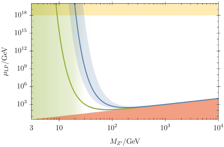
This overall pattern is in sharp contrast to the situation observed in rare -decays, where the anomalies indicate TeV and a TeV-size is vastly separated from the Landau pole. This permits the introduction of additional BSM-interactions to evade the Landau pole, and to secure Higgs stability all the way up to the Planck scale (and possibly beyond) Bause:2021prv.
V Conclusions
The recent data on charm CP-violation (1), taken at face value, together with the measurement of (2), require to accept a huge amount of -spin breaking, or NP below the weak scale. Explaining Eq. (I) indeed poses a challenge to model building, given the low NP scale and the severe constraints from rare decays, mixing, and searches for BSM bosons in dilepton and dijets channels.
We obtain viable explanations of data (I) from a light -boson, , with novel, characteristic patterns in couplings to fermions: successful model benchmarks, see Tab. 1, accidentally couple only to right-handed fermions and are leptophobic (BM IV) or do not have -charges to electrons or muons (BM III). The latter is subject to kinetic mixing at one loop, which requires a non-excessive tuning of the mixing parameter at the level of ten percent. The former is a novel benchmark using a Diophantine construction to maintain anomaly freedom and the absence of one-loop kinetic mixing, since it couples mostly to quarks without introducing new matter fields, derived in App. C.
Models do not couple to top quarks allowing for the top Yukawa to be written down directly. BM III allows also the bottom Yukawa at tree level. We stress that we are not addressing the origin of flavor, which is beyond the scope of this work. Models can also include a dark sector, which can significantly speed up the running such that low scale Landau poles arise which point to a UV-completion as low as a TeV, see Fig. 7. However, in view of the ”the lighter, the safer”-rule a sufficiently light , with details depending on the dark sector, can avoid this.
Model frameworks BM III and BM IV are unique as they are minimal models passing the very many theoretical and experimental constraints. Together with viable variants obtained by swapping charges within one species, such as BM III-s, they are indeed the only, minimal options, inducing CP-violation in the current and an enhanced current, but it cannot be ruled out that further, highly tuned scenarios with cross talk between species may be constructed. Another intriguing feature of the models is that they can simultaneously explain the charm CP-data (I) and the , branching ratios for a around GeV (BM III) or GeV (BM IV), see Sec. III.1, providing a NP-explanation to the long-standing pion form factor puzzle.
Models can be searched for in low mass dijets along the lines of CMS:2019xai or and or -decays and related dark photon searches. The dominant branching ratios are given in Tab. 2. Signatures include enhanced production in , or , and in BM III. If dark fermions are also present signatures as in Fig. 6 with hadrons and invisibles are promising smoking guns. We stress that BM III-s, a variant of BM III with the charges between first and second generation up-type quark singlets flipped, , is equally viable. It has a different phenomenology than the other benchmark models, as it does couple essentially to first generation quarks, the , and neutrinos, hence evades charmonium limits, and could be as light as or possibly below.
All viable models further predict isospin violation and pattern in the CP-asymmetries in hadronic charm decays, see (25), in addition to , which also requires U-spin breaking Grossman:2006jg. Models are tightly constrained by -mixing and -searches into electrons and muons. They can hence signal NP in the next round of data.
Acknowledgements.
We are happy to thank Tommaso Pajero and Stefan Schacht for useful communication, and Alex Gilman for pointing out charmonia bounds for taus and invisibles. This work is supported by the Studienstiftung des Deutschen Volkes (TH), the Bundesministerium für Bildung und Forschung (BMBF) under project number 05H21PECL2 (HG), and the Science and Technology Research Council (STFC) under the Consolidated Grant ST/T00102X/1 (DFL). This work was performed in part at Aspen Center for Physics (GH, DFL), which is supported by National Science Foundation grant PHY-1607611, and was partially supported by a grant from the Simons Foundation (DFL). GH is grateful to the MITP of the PRISMA+ Cluster (Project ID 39083149), for its hospitality and partial support during the completion of this work.Appendix A Amplitudes and observables in SM
The SM decay amplitudes of and its conjugate decay can be written in terms of reduced amplitudes with relative strong phase as
| (54) | ||||
| (55) |
where and due to CKM-unitarity up to a negligible . The amplitude is predominantly induced by tree-level -exchange, whereas originates from higher order contributions including penguin-loops or final-state interactions. Using standard formulas one obtains for the direct CP-asymmetry of decays in the SM
| (56) |
where we neglected contributions of higher order in CKM-ratios . This approximation implies also that the CP-averaged branching ratio is dominated by the term with the leading CKM-factor , .
Expressions for decays are analogous:
| (57) | ||||
| (58) |
In the -spin limit the phase and reduced amplitudes are universal, such as and so on. The observed -spin breaking in the branching ratios can be explained with a flavor-dependent correction , as , at the nominal level of flavor breaking, Brod:2012ud. This -spin breaking in the branching ratios and correspondingly between the leading contributors to the amplitudes implies a shift in the CP-asymmetries e.g. (56) and leads to the modified -spin relation (4).
Appendix B RGE and hadronization
NP effects in charm decays are described within the effective weak Hamiltonian . Operators relevant to a -boson coupling to right-handed quarks read
| (59) | ||||
| (60) |
where refers to the Dirac structures , , and are color indices.
In the following, we address the evolution of the Wilson coefficients at the mass scale,
| (61) |
down to the charm mass scale at leading order in , see Bause:2020obd for details. The CP-violating phase is . Using the anomalous dimension given by Eq. (B1) in Ref. Bause:2020obd, and integrating out degrees of freedom at the –scales, one obtains
| (62) |
where is the evolution matrix from scale to scale . Using Eq. (61) and (62), we obtain
| (63) | ||||
| (64) |
where
| (65) |
for , while
| (66) |
for .
For the computation of the and hadronic matrix elements we employ factorization of currents,
| (67) | ||||
with , is a –quark operator and represent Dirac and color structures while denote quarks. The factor parametrizes the deviation of the true hadronic matrix element from its naïve approximation, . Including these effects the CP-asymmetries become
| (68) | ||||
where we have already used . Furthermore
| (69) | ||||
with
| (70) |
and
| (71) |
In naïve factorization, and , recovering Eq. (D2) from Ref. Bause:2020obd. In the large- limit . We show against in Fig. 8. In naive factorization (red lines) exhibits a strong cancellation around GeV stemming from the numerator of Eq. (70). Comparing with the large- limit (green lines), we observe that this cancellation is only effective in the naïve factorization limit. Taking into account that naïve factorization suffers from sizable uncertainties, blue lines illustrate , in our analysis for light masses we use TeV2.
Appendix C Anomaly cancellation
The gauge anomaly cancellation conditions (ACCs) read Allanach:2018vjg; Bause:2019vpr
| (72) | ||||
| (73) | ||||
| (74) | ||||
| (75) | ||||
| (76) | ||||
| (77) |
In addition, avoiding kinetic mixing at one loop requires Holdom:1985ag; Bause:2020obd
| (78) |
Here, we use the notation and with . First, we focus on those equations that are linear with trace charge matrices, that are Eqs. (72),(73),(74),(75), and (78). Solving them, we find
Setting we avoid kaon constraints and for the BMs III and IV couplings to the top, and arrive at the simple condition
| (79) |
and therefore from Eq. (C) to
| (80) |
Let us work on the remaining ACCs, Eqs. (76) and (77). The non-linear behavior of these equations makes it challenging to solve them. We have already some information about the trace of these matrices, they are zero (80). To solve the problem mathematical relations between , and would be helpful. Noting that for matrices holds
| (81) |
and it follows from that vanishes if one charge vanishes, for instance, ; then Eq. (77) is fulfilled. In general, the charge matrices can then be written as
| (82) |
where are integers. Note that the order of can be changed for each species independently. It remains to solve Eq. (76), which now simply reduces to
| (83) |
We can start exploring this equation by setting . This solution is motivated from the phenomenological point of view because we need small values of lepton charges as well as being disconnected from quark charges. However in this case the system has only the trivial solution because can not be fulfilled for integers. Let us simplify (83) by setting which is motivated by the strong constraints on lepton couplings. We obtain
| (84) |
Two aspects are worth noting from this equation:
- (a)
For any Pythagorean triple , i.e. integers which solve Pythagoras equation , one can find integer triples which solve Eq. (84) by substituting , , and .
- (b)
Any solution to Eq. (84) can be parametrised by integers
(85) (86) (87) The first non-trivial solutions are found to be
(88) and so on, and integer multiples thereof. Note that each term can also have either sign, and that permutations between and are permitted.
Although Eq. (84) gets fully solved by Eqs. (85)-(87), in the following, we illustrate a more practical approach that allows us to run directly into those solutions that accommodate the constraint given by Eq. (34). Let us rewrite (84) as
| (89) |
with and
| (90) |
For illustration, we start with the trivial solution . Using Eq. (89), we obtain
| (91) |
with
| (92) |
Now, the question we should ask is: are there more solutions such as ? One possibility is if a transformation
| (93) |
by a matrix with integer entries , leads invariant Eq. (91) so that we can generate recursively solutions
| (94) |
which could get enlarged while keeping fixed to for this particular case. This matrix needs to satisfy
| (95) |
The solution of this system in terms of is
| (96) | ||||
| (97) | ||||
| (98) |
with four solutions , , , . The smallest integer solution reads
| (99) |
We then find the solutions (94) for any integer . Using leads to
| (100) | ||||
We learn that in order to avoid electron and muon constraints of Eq. (34), we need solutions with . Note that we could have also used a different setup for to get different solutions. In addition, we can also find more solutions by choosing another initial integer triple .
In the phenomenological analysis, we considered the solution for BM IV,
| (101) |
with zero neutrino charges .
Appendix D Kinetic mixing
In this appendix we discuss the naturalness of the gauge-kinetic mixing, occurring due to the parameter as in (35) between the and the photon, or equivalently the and hypercharge gauge boson before electroweak symmetry breaking. Ideally, one would like the RG evolution of this parameter to be technically natural, which means
| (102) |
This would imply that kinetic mixing can naturally be switched off at all scales, or made to remain arbitrarily small.
For theories with the charge configuration (82), as well as the Higgs not carrying a charge, kinetic mixing is natural at one-loop order. If only gauge contributions are taken into account, the naturalness remains intact even at higher loops, which is the result of the symmetry implied by (82). We have verified that this is the case until four loops, using the results of Bednyakov:2021qxa; Davies:2021mnc.
Starting at two-loop order, Yukawa interactions violate the naturalness (102), unless they retain certain flavor textures. If the top quark does not carry charge as in BM IV, the naturalness-violating terms do not feature the top Yukawa coupling at two loops, and are either suppressed by the other, much smaller Yukawas and/or loop factors. Thus, these terms are negligible for the running of , which becomes effectively natural.
However, the naturalness is broken at one loop below the scale where the first field carrying charge is integrated out, i.e. the bottom quark in BM IV.
References
- (1) [LHCb], CERN-EP-2022-163, LHCb-PAPER-2022-024 [arXiv:2209.03179 [hep-ex]].
- (2) R. Aaij et al. [LHCb], Phys. Rev. Lett. 122, no.21, 211803 (2019) doi:10.1103/PhysRevLett.122.211803 [arXiv:1903.08726 [hep-ex]].
- (3) Y. Amhis et al. [HFLAV], Phys. Rev. D 107 (2023) no.5, 052008 doi:10.1103/PhysRevD.107.052008 [arXiv:2206.07501 [hep-ex]].
- (4) S. Schacht, JHEP 03 (2023), 205 doi:10.1007/JHEP03(2023)205 [arXiv:2207.08539 [hep-ph]].
- (5) M. J. Savage, Phys. Lett. B 257 (1991), 414-418 doi:10.1016/0370-2693(91)91917-K
- (6) D. Pirtskhalava and P. Uttayarat, Phys. Lett. B 712, 81-86 (2012) doi:10.1016/j.physletb.2012.04.039 [arXiv:1112.5451 [hep-ph]].
- (7) J. Brod, Y. Grossman, A. L. Kagan and J. Zupan, JHEP 10 (2012), 161 doi:10.1007/JHEP10(2012)161 [arXiv:1203.6659 [hep-ph]].
- (8) G. Hiller, M. Jung and S. Schacht, Phys. Rev. D 87 (2013) no.1, 014024 doi:10.1103/PhysRevD.87.014024 [arXiv:1211.3734 [hep-ph]].
- (9) T. Feldmann, S. Nandi and A. Soni, JHEP 06, 007 (2012) doi:10.1007/JHEP06(2012)007 [arXiv:1202.3795 [hep-ph]].
- (10) R. Bause, H. Gisbert, M. Golz and G. Hiller, Phys. Rev. D 101, no.11, 115006 (2020) doi:10.1103/PhysRevD.101.115006 [arXiv:2004.01206 [hep-ph]].
- (11) Y. Grossman, A. L. Kagan and Y. Nir, Phys. Rev. D 75, 036008 (2007) doi:10.1103/PhysRevD.75.036008 [arXiv:hep-ph/0609178 [hep-ph]].
- (12) J. Brod, A. L. Kagan and J. Zupan, Phys. Rev. D 86, 014023 (2012) doi:10.1103/PhysRevD.86.014023 [arXiv:1111.5000 [hep-ph]].
- (13) W. Altmannshofer, R. Primulando, C. T. Yu and F. Yu, JHEP 04, 049 (2012) doi:10.1007/JHEP04(2012)049 [arXiv:1202.2866 [hep-ph]].
- (14) [HFLAV], Global Fit for mixing (allowing for CP violation), accessed on Oct. 28th, 2022.
- (15) R. Aaij et al. [LHCb], Phys. Rev. Lett. 127 (2021) no.11, 111801 doi:10.1103/PhysRevLett.127.111801 [arXiv:2106.03744 [hep-ex]].
- (16) [LHCb], Rare charm decays at LHCb, Marianna Fontana, Talk at ICHEP 2022.
- (17) H. Gisbert, M. Golz and D. S. Mitzel, Mod. Phys. Lett. A 36 (2021) no.04, 2130002 doi:10.1142/S0217732321300020 [arXiv:2011.09478 [hep-ph]].
- (18) J. Fuentes-Martin, A. Greljo, J. Martin Camalich and J. D. Ruiz-Alvarez, JHEP 11, 080 (2020) doi:10.1007/JHEP11(2020)080 [arXiv:2003.12421 [hep-ph]].
- (19) M. Ablikim et al. [BESIII], Phys. Rev. D 105, no.7, L071102 (2022) doi:10.1103/PhysRevD.105.L071102 [arXiv:2112.14236 [hep-ex]].
- (20) R. Bause, H. Gisbert, M. Golz and G. Hiller, Phys. Rev. D 103 (2021) no.1, 015033 doi:10.1103/PhysRevD.103.015033 [arXiv:2010.02225 [hep-ph]].
- (21) R. Bause, H. Gisbert, M. Golz and G. Hiller, Eur. Phys. J. C 82 (2022) no.2, 164 doi:10.1140/epjc/s10052-022-10113-6 [arXiv:2007.05001 [hep-ph]].
- (22) Y. T. Lai et al. [Belle], Phys. Rev. D 95, no.1, 011102 (2017) doi:10.1103/PhysRevD.95.011102 [arXiv:1611.09455 [hep-ex]].
- (23) D. Wang, Eur. Phys. J. C 83 (2023), 279 doi:10.1140/epjc/s10052-023-11439-5 [arXiv:2207.11053 [hep-ph]].
- (24) P. Ilten, Y. Soreq, M. Williams and W. Xue, JHEP 06, 004 (2018) doi:10.1007/JHEP06(2018)004 [arXiv:1801.04847 [hep-ph]].
- (25) A. M. Sirunyan et al. [CMS], Phys. Rev. Lett. 123, no.23, 231803 (2019) doi:10.1103/PhysRevLett.123.231803 [arXiv:1905.10331 [hep-ex]].
- (26) B. A. Dobrescu and F. Yu, [arXiv:2112.05392 [hep-ph]].
- (27) B. A. Dobrescu and C. Frugiuele, Phys. Rev. Lett. 113, 061801 (2014) doi:10.1103/PhysRevLett.113.061801 [arXiv:1404.3947 [hep-ph]].
- (28) A. Aranda and C. D. Carone, Phys. Lett. B 443, 352-358 (1998) doi:10.1016/S0370-2693(98)01309-4 [arXiv:hep-ph/9809522 [hep-ph]].
- (29) B. Batell, J. L. Feng, M. Fieg, A. Ismail, F. Kling, R. M. Abraham and S. Trojanowski, Phys. Rev. D 105, no.7, 075001 (2022) doi:10.1103/PhysRevD.105.075001 [arXiv:2111.10343 [hep-ph]].
- (30) D. C. Bailey and S. Davidson, Phys. Lett. B 348, 185-189 (1995) doi:10.1016/0370-2693(95)00052-M [arXiv:hep-ph/9411355 [hep-ph]].
- (31) S. Cheng, A. Khodjamirian and A. V. Rusov, Phys. Rev. D 102, no.7, 074022 (2020) doi:10.1103/PhysRevD.102.074022 [arXiv:2007.05550 [hep-ph]].
- (32) Workman, R. L. et al. [Particle Data Group], PTEP 2022, 083C01 doi:10.1093/ptep/ptac097
- (33) C. Bruch, A. Khodjamirian and J. H. Kuhn, Eur. Phys. J. C 39, 41-54 (2005) doi:10.1140/epjc/s2004-02064-3 [arXiv:hep-ph/0409080 [hep-ph]].
- (34) R. Baldini Ferroli, A. Mangoni and S. Pacetti, Phys. Rev. C 98, no.4, 045210 (2018) doi:10.1103/PhysRevC.98.045210 [arXiv:1611.04437 [hep-ph]].
- (35) M. Fabbrichesi, E. Gabrielli and G. Lanfranchi, doi:10.1007/978-3-030-62519-1 [arXiv:2005.01515 [hep-ph]].
- (36) R. Bause, G. Hiller, T. Höhne, D. F. Litim and T. Steudtner, Eur. Phys. J. C 82, no.1, 42 (2022) doi:10.1140/epjc/s10052-021-09957-1 [arXiv:2109.06201 [hep-ph]].
- (37) R. Aaij et al. [LHCb], Phys. Rev. Lett. 124, no.4, 041801 (2020) doi:10.1103/PhysRevLett.124.041801 [arXiv:1910.06926 [hep-ex]].
- (38) A. Bednyakov and A. Pikelner Phys. Rev. Lett. 127 no.4, 041801 (2021) doi:10.1103/PhysRevLett.127.041801 [arXiv: 2105.09918 [hep-ph]].
- (39) J. Davies, F. Herren and A. E. Thomsen, JHEP 01 051 (2022) doi:10.1007/JHEP01(2022)051 [arXiv:2110.05496 [hep-ph]]
- (40) M. Campajola et al. [Belle II], [arXiv:2208.01101 [hep-ex]].
- (41) M. Ablikim et al. [BESIII], [arXiv:2209.13893 [hep-ex]].
- (42) J. P. Lees et al. [BaBar], [arXiv:1702.03327 [hep-ex]].
- (43) R. Bause, M. Golz, G. Hiller and A. Tayduganov, Eur. Phys. J. C 80, no.1, 65 (2020) [erratum: Eur. Phys. J. C 81, no.3, 219 (2021)] doi:10.1140/epjc/s10052-020-7621-7 [arXiv:1909.11108 [hep-ph]].
- (44) B. C. Allanach, J. Davighi and S. Melville, JHEP 02, 082 (2019) [erratum: JHEP 08, 064 (2019)] doi:10.1007/JHEP02(2019)082 [arXiv:1812.04602 [hep-ph]].
- (45) B. Holdom, Phys. Lett. B 166, 196-198 (1986) doi:10.1016/0370-2693(86)91377-8