Design of Convolutional Extreme Learning Machines for Vision-Based Navigation Around Small Bodies

Mattia Pugliatti Note: Ph.D. Student, Department of Aerospace Science and Technology, Via La Masa 34, mattia.pugliatti@polimi.it Affiliation: Politecnico di Milano, 20156, Milan, Italy Francesco Topputo Note: Full Professor, Department of Aerospace Science and Technology, Via La Masa 34, francesco.topputo@polimi.it, AIAA senior member Affiliation: Politecnico di Milano, 20156, Milan, Italy

Abstract

Deep learning architectures such as convolutional neural networks are the standard in computer vision for image processing tasks. Their accuracy however often comes at the cost of long and computationally expensive training, the need for large annotated datasets, and extensive hyper-parameter searches. On the other hand, a different method known as convolutional extreme learning machine has shown the potential to perform equally with a dramatic decrease in training time. Space imagery, especially about small bodies, could be well suited for this method. In this work, convolutional extreme learning machine architectures are designed and tested against their deep-learning counterparts. Because of the relatively fast training time of the former, convolutional extreme learning machine architectures enable efficient exploration of the architecture design space, which would have been impractical with the latter, introducing a methodology for an efficient design of a neural network architecture for computer vision tasks. Also, the coupling between the image processing method and labeling strategy is investigated and demonstrated to play a major role when considering vision-based navigation around small bodies.

1 Introduction

Missions towards small bodies, such as asteroids and comets, are becoming increasingly interesting for national space agencies, companies, and smaller players such as research centers and universities [1]. From a scientific point of view, these bodies gather valuable information on the Solar System’s primordial state. Their heterogeneous distribution makes them abundantly available for resource exploitation and easily accessible from Earth, which in turn might pose an existential threat to human activities and an opportunity for technology demonstration.

The capability to autonomously navigate around a known celestial body is of paramount importance to enable any autonomous decision-making process on-board a spacecraft [1]. When considering both the proximity environment of a small body and the navigation sensors available on the market, cameras are usually preferred as they are light, compact, and have low power demand. For these reasons, the use of passive cameras, in combination with Image Processing algorithms, provides compelling navigation performances with cost-effective hardware.

A promising family of Image Processing methods is represented by data-driven algorithms, especially those making use of deep learning. In this context, traditional deep learning architectures like Convolutional Neural Network and its variants have demonstrated their exceptional capability to extract high-level features from images and process their nonlinear mapping with labels, representing the state of the art in computer vision for several tasks [2]. On the other hand, Convolutional Neural Networks often need a large amount of data for training, which occurs via Gradient Descent methods and requires substantial computational resources [2].

An opposite approach to deep architectures and learning via Gradient Descent exists, which in some cases has been demonstrated to perform similarly or better. Extreme Learning Machine is a theoretical formulation of a learning strategy that has been first introduced in [3] and later organized more consistently first in [4] and then in [5]. In these works Extreme Learning Machine theory is applied to single layers feed-forward networks whose weights and biases are initialized randomly. Training happens using a Least Square method to adjust the weights of the connections between the single hidden layer and the output one. Because Least Square is an order of magnitude faster than Gradient Descent, training happens extremely fast. The idea is that with enough randomized neurons in the hidden layers, a network would be capable to generate a multi-dimensional basis that can be used to map the nonlinear relationship between input and labels. Extreme Learning Machine is demonstrated to perform similarly or better than deep architectures [3, 4, 5], requiring only a fraction of their training time.

At the same time Extreme Learning Machine concepts were being formalized and used, the pivotal work in [6] stressed the unexpected performance achieved with Convolutional Neural Network when using random weights and biases in the convolutional kernels. The authors prove that: 1) A surprising fraction of performance in a Convolutional Neural Network can be contributed by the intrinsic properties of the architecture alone and not from the learning algorithm used; 2) Convolutional pooling architectures can be frequency selective and translation invariant, even when random weights are used; 3) A methodology that uses randomized Convolutional Neural Network to search the hyper-parameters within the architecture design space perform inherently better than traditional approaches. By sidestepping the time-consuming learning process, and only focusing on those architectures with superior hierarchical structures, an order of magnitude speedup in the training process is obtained.

These two research lines come together in [7], which extends the Extreme Learning Machine theory to Convolutional Neural Network with randomized kernels, introducing the concept of Convolutional Extreme Learning Machine for computer vision tasks. The convolutional layers of a Convolutional Neural Network are set with random weights and biases, up to the fully connected layer, whose connections with the output layer are treated as an Extreme Learning Machine architecture and solved with a Least Square method. Similarly to Extreme Learning Machine, Convolutional Extreme Learning Machine achieves extremely fast training and accuracies that may be similar to those of Convolutional Neural Network.

Several other works using Convolutional Extreme Learning Machine architectures and training strategies are present in the literature. A thorough, systematic review of these is illustrated in [8]. Interestingly, no prior work has been focused on the adoption of Convolutional Extreme Learning Machine for on-board Image Processing of celestial bodies.

When considering images of a small body taken from a navigation camera, the scenery is relatively simple when compared to other computer vision domains. The background and foreground are clearly distinguishable, and the surface variations are only due to morphological characteristics (i.e. craters, boulders, etc.) which only vary under illumination conditions. This domain is fundamentally simpler than that of typical computer vision applications in urban environments, which need to account for a large variety of commonly used objects, where deep architectures are the state of the art [2]. Moreover, previous findings in [9] hint to the fact that the filtering capabilities Convolutional Neural Networks on images of a small body are critical in pushing the performance compared to traditional methods.

Pivoting on these prior works and the existing gaps in the literature, in this paper the authors attempt to answer three fundamental questions, namely: 1) Although Convolutional Neural Network are superior over complex scenery, can simpler methods perform better when it comes to analyzing images of small bodies?; 2) As suggested in [6], can a methodology be developed to bootstrap the training of Convolutional Neural Network exploiting the capability of Convolutional Extreme Learning Machine to identify the most promising architectures?; 3) Which is the best labeling strategy and reference frame to be used when considering a visual-based navigation application around a small body?

In this work, Convolutional Extreme Learning Machine is thus investigated as a possible alternative to Convolutional Neural Network for autonomous vision-based navigation systems around small bodies. This is done with an extensive analysis considering 4 different small body shapes and 5 different labeling strategies, for a total of 20 scenarios, each of which is examined with 4 different Image Processing methods, resulting in tens of thousands of different architectures explored. Such efficient exploration of the architecture design space is possible thanks to the extremely fast training time of Convolutional Extreme Learning Machine, which is orders of magnitude faster than that of Convolutional Neural Network [7]. It is also demonstrated that the labeling strategy and reference frame play a crucial role during training and significantly affect the performance of the methods considered. We believe that Convolutional Extreme Learning Machine can represent, with the proper labeling strategy, a promising alternative in space imagery, especially the one related to small bodies.

The rest of the paper is organized as follows. In Section 2 the three pillars sustaining the methodology are discussed in detail. These are the dataset generation, the preprocessing pipeline of the image-label pairs, and the description of the Image Processing methods developed and used in this paper. The performance of these methods is then compared extensively in Section 3 while conclusions, and future works are discussed in Section 4.

2 Methodology

2.1 Dataset generation

In this section, the dataset generation procedure is illustrated. Four small bodies are considered: 65803 Didymos, 103P/Hartley, 21 Lutetia and 67P/Churyumov–Gerasimenko. Using the same methodology illustrated in [10], artificial morphological features such as boulders and craters are inserted into the shape models of these bodies.

For each body, a total of $17500$ grayscale images are rendered in Blender¹¹ 1 https://www.blender.org/, retrieved 25 August 2022.. These are split into training, validation, and test sets respectively made of $7500$ , $5000$ , and $5000$ images. As illustrated in Fig. 1, these sets are randomly distributed across a cloud of points around the body in what is defined as the $W$ reference frame. This reference frame is an inertially fixed reference frame, centered on the Center of Mass of the body, with the $X$ -axis oriented towards the projection of the Sun in the body equatorial plane and the $Z$ -axis as the north pole of the body. Another reference frame that is used in this paper is the $AS$ one, whose axes are fixed to the body surface and are obtained from a rigid rotation around the $Z$ -axis of the $W$ reference frame. The points in Fig. 1 are distributed with range $\rho\in[5,\ 30]\ {\rm km}$ , azimuth $\phi_{1}\in[-90,\ 90]\ {\rm deg}$ and elevation $\phi_{2}\in[-45,\ 45]\ {\rm deg}$ in the $W$ reference frame. These settings have been arbitrarily chosen as reasonable assumptions for a realistic close-proximity scenario for a mission with a passive sensor. Since each dataset is composed of the same set of points across different bodies, uniform scaling is applied to each one to make sure that different body sizes are all filling the Field Of View around $5$ km.

Refer to caption — Figure 1: Cloud of $17500$ points used for training, validation, and test of the Image Processing methods.

To generate the $8$ -bit grayscale images, a camera with a $10\times 10$ deg Field Of View and a sensor of $1024\times 1024$ pixel is considered. All images are rendered assuming ideal pointing towards the Center of Mass. From an optical-navigation point of view, images can be represented by different sets of labels. Five of these are considered in this work to investigate the influence of this choice on the performance of the Image Processing methods. The first one is represented by optical observables linked with geometrical quantities directly detectable from images. In this work, these are:

\bm{\delta}=\bm{CoF}-\bm{CoB}\quad,\quad\rho

(1)

where $\bm{\delta}$ is the difference in pixels between the Center of Brightness and Center of Figure of the body projected in the image plane and $\rho$ is the range from the Center of Mass. These quantities can be used to generate a position estimate in the camera frame, which can be transformed in $W$ or $AS$ by simulating on-board attitude determination from a star-tracker alongside the assumption of knowledge of the rigid rotation between the inertially fixed reference frames used by star-tracker and the $W$ or $AS$ frames. The second and third sets are represented by the spacecraft position respectively in spherical and cartesian coordinates in the $W$ frame. Similarly, the fourth and fifth sets are represented by the same coordinates in the $AS$ frame.

By combining the 4 different small bodies with these 5 different labeling strategies, a total of 20 cases are considered in this paper. The notation used to distinguish between these cases is summarized in Tab. 1.

Table 1: Notation used for the datasets used in this work.

ID	Body	Frame	Labels	Notation
1	D	-	$\bm{\delta},\rho$	D1
2	H	-	$\bm{\delta}$ , $\rho$	H1
3	L	-	$\bm{\delta}$ , $\rho$	L1
4	P	-	$\bm{\delta}$ , $\rho$	P1
5	D	$AS$	$\phi_{1},\phi_{2},\rho$	D2
6	H	$AS$	$\phi_{1},\phi_{2},\rho$	H2
7	L	$AS$	$\phi_{1},\phi_{2},\rho$	L2
8	P	$AS$	$\phi_{1},\phi_{2},\rho$	P2
9	D	$AS$	$X,Y,Z$	D3
10	H	$AS$	$X,Y,Z$	H3
11	L	$AS$	$X,Y,Z$	L3
12	P	$AS$	$X,Y,Z$	P3
13	D	$W$	$\phi_{1},\phi_{2},\rho$	D4
14	H	$W$	$\phi_{1},\phi_{2},\rho$	H4
15	L	$W$	$\phi_{1},\phi_{2},\rho$	L4
16	P	$W$	$\phi_{1},\phi_{2},\rho$	P4
17	D	$W$	$X,Y,Z$	D5
18	H	$W$	$X,Y,Z$	H5
19	L	$W$	$X,Y,Z$	L5
20	P	$W$	$X,Y,Z$	P5

2.2 Preprocessing

After the dataset generation step, a total of $70000$ , $1024\times 1024$ grayscale images with ideal pointing towards the Center of Mass of each body are obtained. These images, however, cannot be used directly as input of the Image Processing methods considered in this work for three main reasons.

First, the original image resolution is too high. Due to hardware limitations, image size needs to be reduced. This is typical of the data-driven Image Processing methods used, which could encounter memory or processing saturation issues if working with images at native resolutions. Second, the ideal pointing assumed during rendering simplifies image generation but causes poor variability of the input-label relationship, which can cause poor generalization capability of the Image Processing methods. Third, rendered images are ideal, thus far from realistic camera acquisitions.

All three issues are addressed together in a unique preprocessing pipeline which is a novel contribution of this work. The pipeline transforms an image and its associated labels from a geometrical and rendering space referred to as $\mathbb{S}_{0}$ into a new space $\mathbb{S}_{2}$ that can be efficiently used by data-driven Image Processing algorithms. A sketch of the pipeline is illustrated in Fig. 2 for clarity.

The starting point of the pipeline is the image rendered in Blender, which by definition belongs to $\mathbb{S}_{0}$ space. The image is binarized using the Otsu method [11] and a simple blob analysis is performed to compute the Center of Brightness (represented by the yellow point in Fig. 2) and the bounding box $\Gamma$ (defined by two corner coordinates $\Gamma_{1},\Gamma_{2}$ , its width $\Gamma_{3}$ , and height $\Gamma_{4}$ ). All these quantities are computed in the $UV$ frame [12], which is considered in the image plane as centered on the top-left corner of the image.

Cropping is performed around $\Gamma$ to transform the image to a $\Gamma_{3}\times\Gamma_{4}$ snippet. Because the Image Processing methods considered in this work assume fixed-size inputs, the variable-size snippet needs to be transformed into a fixed-size one.

The upper closest possible value $\gamma$ between the largest size of $\Gamma_{3}\times\Gamma_{4}$ and $128$ , $256$ , $512$ , or $1024$ is computed. Once the target size is determined, padding is performed using two parameters, $\alpha_{u}$ , and $\alpha_{v}$ , which are randomly generated. These represent the necessary integer lengths that need to be added to $\Gamma$ and are chosen respectively as $0\leq\alpha_{u}\leq\gamma-\Gamma_{3}$ and $0\leq\alpha_{v}\leq\gamma-\Gamma_{4}$ . After random padding, the image is said to be transformed in $\mathbb{S}_{1}$ space. Note that the padding is performed by re-using the same pixels from the image defined in $\mathbb{S}_{0}$ or by introducing zero-pixels values (using the nearest criteria) whenever this is not possible. When passing from $\mathbb{S}_{0}$ to $\mathbb{S}_{1}$ also the labels linked to the image need to be transformed, resulting in a change in the $\bm{CoB}$ and $\bm{CoF}$ coordinates:

\bm{CoB}^{\mathbb{S}_{1}}=\bm{CoB}^{\mathbb{S}_{0}}-\begin{bmatrix}\Gamma_{1}\\ \Gamma_{2}\end{bmatrix}+\begin{bmatrix}\alpha_{u}\\ \alpha_{v}\end{bmatrix}\quad,\quad\bm{CoF}^{\mathbb{S}_{1}}=\bm{CoF}^{\mathbb{S}_{0}}-\begin{bmatrix}\Gamma_{1}\\ \Gamma_{2}\end{bmatrix}+\begin{bmatrix}\alpha_{u}\\ \alpha_{v}\end{bmatrix}

(2)

while the other labels remain unchanged: $\bm{\delta}^{\mathbb{S}_{1}}=\bm{\delta}^{\mathbb{S}_{0}}$ ; $\rho^{\mathbb{S}_{1}}=\rho^{\mathbb{S}_{0}}$ ; $[X,Y,Z]^{\mathbb{S}_{1}}=[X,Y,Z]^{\mathbb{S}_{0}}$ ; and $[\phi_{1},\phi_{2}]^{\mathbb{S}_{1}}=[\phi_{1},\phi_{2}]^{\mathbb{S}_{0}}$ . Noise is then added to the image, which is resized to a $128\times 128$ resolution, transforming it in $\mathbb{S}_{2}$ space. The noise step is optional for images in the datasets, while in an operational scenario it would be avoided. When passing from $\mathbb{S}_{1}$ to $\mathbb{S}_{2}$ the labels are transformed as follows:

\bm{CoB}^{\mathbb{S}_{2}}=\bm{CoB}^{\mathbb{S}_{1}}\frac{128}{\gamma}\quad,\quad\bm{CoF}^{\mathbb{S}_{2}}=\bm{CoF}^{\mathbb{S}_{1}}\frac{128}{\gamma}\quad,\quad\bm{\delta}^{\mathbb{S}_{2}}=\bm{\delta}^{\mathbb{S}_{1}}\frac{128}{\gamma}

(3)

\rho^{\mathbb{S}_{2}}=\rho^{\mathbb{S}_{1}}\frac{128}{\gamma}

(4)

[X,Y,Z]^{\mathbb{S}_{2}}=[X,Y,Z]^{\mathbb{S}_{1}}\frac{128}{\gamma}

(5)

while $\phi_{1}$ and $\phi_{2}$ remain unchanged: $[\phi_{1},\phi_{2}]^{\mathbb{S}_{2}}=[\phi_{1},\phi_{2}]^{\mathbb{S}_{1}}$ . Combining Equation 2 with Equation 3, Equation 4, and Equation 5 it is possible to transform the image-label pairs for all the datasets in Tab. 1. All the Image Processing methods used in this work use the image-label pairs in $\mathbb{S}_{2}$ space, which need transformation to $\mathbb{S}_{0}$ for on-board usage. The methods working on the datasets labeled with cartesian and polar coordinates either in the $AS$ or $W$ reference frames generate directly a position estimate as:

\bm{p}^{i,\mathbb{S}_{0}}_{est}=\frac{\gamma}{128}\begin{bmatrix}X\\ Y\\ Z\end{bmatrix}^{i,\mathbb{S}_{2}}_{est}

(6)

\bm{p}^{i,\mathbb{S}_{0}}_{est}=\Omega\left(\begin{bmatrix}\phi_{1}\\ \phi_{2}\\ \rho\frac{\gamma}{128}\end{bmatrix}^{i,\mathbb{S}_{2}}_{est}\right)

(7)

where $i$ reflects the reference frame used, and $\Omega$ is the transformation function from spherical to cartesian coordinates. On the other hand, the methods working with the ( $\bm{\delta},\rho$ ) labels need intermediate steps to generate a position estimate. In inference, these methods generate the following optical observables:

\bm{o}^{uv,\mathbb{S}_{0}}_{est}=\begin{bmatrix}{CoF}^{\mathbb{S}_{0}}_{est,u}\\ {CoF}^{\mathbb{S}_{0}}_{est,v}\\ 1\end{bmatrix}=\begin{bmatrix}{CoB}^{\mathbb{S}_{0}}_{u}+{\delta_{u}}^{\mathbb{S}_{2}}\frac{\gamma}{128}\\ {CoB}^{\mathbb{S}_{0}}_{v}+{\delta_{v}}^{\mathbb{S}_{2}}\frac{\gamma}{128}\\ 1\end{bmatrix}\quad,\quad\rho^{\mathbb{S}_{0}}_{est}=\rho^{\mathbb{S}_{2}}\frac{\gamma}{128}

(8)

where $\bm{\delta}^{\mathbb{S}_{2}}$ and $\rho^{\mathbb{S}_{2}}$ are output of the Image Processing methods while $\bm{CoB}^{\mathbb{S}_{0}}$ and $\gamma$ are parameters computed during the image preprocessing algorithm. In this work, the latter quantities are computed offline, however, it is noted that the algorithm can work also online during inference to prepare any incoming image with the proper format for the application of the Image Processing method. The observable vector $\bm{o}^{uv,\mathbb{S}_{0}}_{est}$ is transformed from the $UV$ reference frame which express pixel coordinates on the image, to the Image Plane reference frame using the inverse of the camera calibration matrix $\bm{K^{-1}}$ [12]:

\bm{o}^{ImP}_{est}=\bm{K^{-1}}\bm{o}^{uv,\mathbb{S}_{0}}_{est}

(9)

The $\bm{o}^{ImP}_{est}$ vector is then transformed into a Line of Sight vector in the $CAM$ reference frame. Using the attitude quaternion of the spacecraft (which is assumed to be known from attitude determination from a Star-tracker) and assuming to know the rigid rotation between the inertial reference frame used by the star-tracker and a known asteroid frame, this Line of Sight is transformed with the use of $\rho^{\mathbb{S}_{0}}_{est}$ into a position estimate in $W$ reference frame:

\bm{p}^{W,\mathbb{S}_{0}}_{est}=\bm{q}_{CAM\rightarrow W}\bm{p}^{CAM}_{est}

(10)

In this work, the $W$ frame is used for simplicity and no error is simulated on the attitude quaternion.

2.3 Image Processing

In this section, the Image Processing methods are described in detail with a standardized notation, illustrated in the architecture outlined in Fig. 3. The input $\bm{X}$ is represented by a $128\times 128\times N$ tensor while the output $\bm{Y}$ is a vector or matrix whose elements represent the specific labels associated with each image or tensor.

To simplify the discussion, the architecture is conceptually divided into two main portions: the encoder and the head. In the first one, a hierarchical sequence of convolutions, activation functions, and pooling operations are performed to extract spatial information which is synthesized in the last layer in a latent tensor represented in orange in Fig. 3. Such 3D tensor is flattened into a 2D vector referred to as the fully connected layer which constitutes the first layer of the head of the architecture. In this portion, several hidden layers may or may not be introduced before the output layer. A network is therefore established to map the connection between the neurons from the fully connected layer, which embeds spatial information extracted from the image in the latent space, and the output layer, which expresses the desired output label of the architecture.

In this work, convolutional layers are driven by weights and biases that only influence the kernels used in the convolution operations. On the other hand, the weights and biases of the head are representing the influence of the neuron connections between the fully connected and output layer. In this work, it is important to consider these two sets of weight and biases separately, since depending on the training strategy, they are handled differently. The former will be referred to as $\bm{W}$ and $\bm{b}$ , the latter to $\bm{\beta}$ and $\bm{\beta_{0}}$ . The set of weights and biases of the entire architecture defines the set of parameters referred to as $\bm{\theta}=\left(\bm{W,\;b,\;\beta,\;\beta_{0}}\right)$ . Another parameter used to describe the architecture is represented by $\bm{\Theta}$ which reflects the set of architectural and training choices often referred to as hyper-parameters.

Within this context, to find an Image Processing method which performs well means to find the best desirable sets of $\bm{\Theta}$ and $\bm{\theta}$ which optimize predefined metrics. Training an architecture can be reduced to a parameter estimation problem with a double nested optimization loop. During training, both architectural and training choices (global parameters) and inner weights and biases (local parameters) need to be found out through data. When these are found, they are frozen and at inference the architecture can be considered as a function $\pi$ (parameterized by $\bm{\Theta}$ and $\bm{\theta}$ ) on the input tensor $\bm{X}$ that generate an output vector $\bm{Y}$ :

\bm{Y}=\pi_{\Theta}\left(\bm{X}|\bm{\theta}\right)

(11)

Now that a shared nomenclature is established, the characteristics of the four Image Processing methods are described in details.

2.3.1 Convolutional Neural Network

In a Convolutional Neural Network the architecture in Fig. 3 is treated as a neural network whose local parameters $\bm{\theta}$ are found using Gradient Descent optimization algorithms. With Gradient Descent all parameters $\bm{\theta}$ are let to vary during training. Several strategies exist depending on the number of images $N_{i}$ considered in order to perform an update of $\bm{\theta}$ . If $N_{i}=1$ the optimization is referred to as Stochastic Gradient Descent; if $N_{i}=N$ ( $N=7500$ in this work) as Gradient Descent; if $1<N_{i}<N$ it is referred to as Mini-Batch Gradient Descent. The use of batches makes it possible to load and process smaller tensors, decreasing the computational load and memory while increasing convergence speed, both of which are issues of the Stochastic Gradient Descent and Gradient Descent, respectively. The batch size is thus often an important design choice when training a Convolutional Neural Network.

All the Gradient Descent-based methods are structured in a two-phase process. First, a forward pass is executed by a specific network defined by $\bm{\theta}$ to generate an output. The comparison between such output and its ground-truth value is quantified by a loss metric, which in turn is fundamental in evaluating the performance of the network as well as to determine the necessary adjustments to $\bm{\theta}$ for improvement. These are determined from the computation of the gradient, that is estimated in a backward pass in the network followed by an update of $\bm{\theta}$ to be used in the next iteration. These two passages, especially the last, are computationally expensive, making the training a laborious procedure. A possible way to reduce the training time is to avoid the backward pass, that also require a different optimization scheme.

2.3.2 Convolutional Extreme Learning Machine

A Convolutional Extreme Learning Machine removes the need for a backward pass by solving the optimization problem on the connections between the last hidden layer and the output layer of the architecture.

In this work, the architecture and initialization of Convolutional Extreme Learning Machine are the same as the one of a Convolutional Neural Network. However, greater importance is given in the Convolutional Extreme Learning Machine on the random distribution of the $W$ eightscnn and $\bm{b}$ of the kernels and of $\bm{\beta_{0}}$ . Once they are randomly initialized when the architecture is generated, they are frozen and are not changed during training. This is not the same for $W$ eightscelm, that are the only ones changed during training. Given a set of true input-output samples $\left(\bm{X},\bm{T}\right)$ , the forward pass of the input into the network generates a hidden layer output matrix $H$ right before the output layer:

\bm{H}=\begin{bmatrix}\bm{h}(\bm{x}_{1})\\ \vdots\\ \bm{h}(\bm{x}_{N})\\ \end{bmatrix}=\begin{bmatrix}h_{1}(\bm{x}_{1})&\ldots&h_{L}(\bm{x}_{1})\\ \vdots&\ddots&\vdots\\ h_{1}(\bm{x}_{N})&\ldots&h_{L}(\bm{x}_{N})\\ \end{bmatrix}

(12)

where $L$ is the dimension of the hidden layer before the output one, represented by the number of neurons in the layer. The training data target matrix is then defined as:

\bm{T}=\begin{bmatrix}\bm{t}_{1}\\ \vdots\\ \bm{t}_{N}\\ \end{bmatrix}=\begin{bmatrix}t_{11}&\ldots&t_{1m}\\ \vdots&\ddots&\vdots\\ t_{N1}&\ldots&t_{Nm}\\ \end{bmatrix}

(13)

To find the best set of weights $\bm{\beta}$ that matches the matrix $\bm{T}$ , the following optimization problem shall be solved [7]:

\text{Minimize}:\left\|\bm{\beta}\right\|^{2}_{2}+C\left\|\bm{H\beta}-\bm{T}\right\|^{2}_{2}

(14)

that is a regularized least square that depends on the $C$ coefficient. The inclusion of first term regarding the minimization of the weights vector $\bm{\beta}$ increases the stability and improves generalization capabilities [4]. The minimization problem can be solved in an efficient way as:

\beta=\left\{\begin{matrix}\bm{H}^{T}\left(\frac{\bm{I}}{C}+\bm{HH}^{T}\right)^{-1}\bm{T},\quad\text{if}\;N\leq L\\ \left(\frac{\bm{I}}{C}+\bm{H}^{T}\bm{H}\right)^{-1}\bm{H}^{T}\bm{T},\quad\text{if}\;N>L\end{matrix}\right.

(15)

Since the remaining weights and biases ( $\bm{W}$ , $\bm{b}$ , and $\bm{\beta}_{0}$ ), are randomly fixed at initialization and are never changed, there is no need for a backward pass. Only the forward pass and the Least Square problem need to be processed, which makes the training of a Convolutional Extreme Learning Machine architecture much faster than the one of a Convolutional Neural Network. Note that in this work $\mathbf{\beta}_{0}$ is not considered in the Convolutional Extreme Learning Machine architecture.

2.3.3 Hybrid Convolutional Extreme Learning Machine

By combining the design of the Convolutional Neural Network and the one of the Convolutional Extreme Learning Machine, the capability of a hybrid Image Processing method is also investigated.

In the Hybrid Convolutional Extreme Learning Machine, transfer learning is used to get the weights and biases of the kernels from the encoder of a previously trained Convolutional Neural Network architecture, while the head is trained using the Least Square method, as in the Convolutional Extreme Learning Machine paradigm. Two Image Processing methods have been designed with this strategy: one that uses the encoder from the best Convolutional Neural Network architecture for that dataset (referred to Hybrid Convolutional Extreme Learning Machine), and one that uses the encoder from the best Convolutional Neural Network architecture for that reference frame (referred to Hybrid Convolutional Extreme Learning Machine 3). In Fig. 4 the schematic difference between the three architectures used in this work is illustrated.

2.3.4 Training

In this section, the strategy to train the Image Processing methods is described. The architecture of each method is generated following a rigid procedural methodology to define the parameters of $\Theta$ . A schematic of the procedure is illustrated in Fig. 5.

To begin with, a great number of Convolutional Extreme Learning Machine architectures are initialized following the same rules for each dataset. The encoder of each architecture is designed with a hierarchical structure [6]. While going deeper from input to the fully connected layer, the starting $128\times 128\times 1$ tensor is squeezed; its size $s_{i}$ is halved as function of the depth level $i$ as $s_{i}=2^{7-i}$ while its depth is doubled starting from an arbitrary value of $16$ .

Each depth level $i$ is made up of the consecutive application of a convolution, activation function, and pooling operation. The convolutions are performed with $3\times 3$ kernels while the number of kernels $n_{i}^{ker}$ used at each depth is set to increase exponentially as:

n_{i}^{ker}=2^{3+i}\qquad n_{0}^{ker}=1

(16)

The number of weights and biases at each depth level of the encoder can thus be determined:

n_{i}^{W}=9n_{i}^{ker}n_{i-1}^{ker}\quad,\quad n_{i}^{b}=n_{i}^{ker}

(17)

From a network as deep as 1 level to one as deep as 5, the cumulative number of parameters defining the weights and biases of the kernels in the encoder is respectively $160$ , $4800$ , $23296$ , $97152$ , and $392320$ . Similarly, also the number of weights and biases of the head can be determined. Since the number of neurons in the fully connected layer depends on the depth level as $n_{i}^{fc}=s_{i}^{2}n_{i}^{ker}$ , the number of $\bm{\beta}$ and $\bm{\beta}_{0}$ of the head is computed as:

n_{i}^{\beta}=n_{i}^{fc}n_{o}\quad,\quad n_{i}^{\beta_{0}}=n_{o}

(18)

where $n_{0}$ is the number of neurons composing the output. For improved handling of the labels, whenever the ( $\phi_{1},\phi_{2},\rho$ ) labels are considered the azimuth angle $\phi_{1}$ is transformed in the adimensional $\left(sin\phi_{1},cos\phi_{1}\right)$ pair. $n_{0}$ is thus equal to $3$ in all datasets but those for which spherical coordinates are used as labels, for which $n_{0}=4$ . An example of a $5$ layers architecture is illustrated in Tab. 2 with a parameter count divided per depth.

Table 2: Example of a 5 layers architecture with a 3 output layer.

Layer name	Layer type	Output Shape	Param $\#$
I	InputLayer	(None, 128, 128, 1)	0
C1	Conv2D	(None, 128, 128, 16)	160
A1	Activation	(None, 128, 128, 16)	0
P1	Pooling	(None, 64, 64, 16)	0
C2	Conv2D	(None, 64, 64, 32)	4640
A2	Activation	(None, 64, 64, 32)	0
P2	Pooling	(None, 32, 32, 32)	0
C3	Conv2D	(None, 32, 32, 64)	18496
A3	Activation	(None, 32, 32, 64)	0
P3	Pooling	(None, 16, 16, 64)	0
C4	Conv2D	(None, 16, 16, 128)	73856
A4	Activation	(None, 16, 16, 128)	0
P4	Pooling	(None, 8, 8, 128)	0
C5	Conv2D	(None, 8, 8, 256)	295168
A5	Activation	(None, 8, 8, 256)	0
P5	Pooling	(None, 4, 4, 256)	0
FC	Flattening	(None, 4096)	0
O	Dense	(None, 3)	12291

Having defined a procedural set of rules to generate each architecture, these are generated with the hyper-parameters $\Theta$ summarized in Tab. 3.

Table 3: Sets of

\bm{\Theta}

explored for Convolutional Extreme Learning Machine and Convolutional Neural Network methods.

Parameter	Symbol	Description	Possible values
Number of layers	$d$	Number of hidden layers in the architecture	1, 2, 3, 4, 5
Kernel distribution	$K_{d}$	Random distribution of the weight and biases of the kernels	Random Uniform (-1,1), Random Normal (0, 1), Orthogonal
Activation function	$A$	Activation function used after the convolution operation	Normalized Rectified Linear Unit, Rectified Linear Unit, hyperbolic tangent, none
Pooling strategy	$P$	Pooling strategy after the activation function	Mean, Max
Regularization coefficient	$C$	Regularization coefficient of Equation 14	$10^{-4}$ , $10^{-3}$ , $10^{-2}$ , $10^{-1}$ , $10^{0}$ , $10^{1}$ , $10^{2}$ , $10^{3}$ , $10^{4}$
Batch size	$N$	Batch size used in the Mini-Batch Gradient Descent	64, 128, 256
Learning rate	$lr$	Learning rate used in the Mini-Batch Gradient Descent	$10^{-1}$ , $10^{-2}$ , $10^{-3}$ , $10^{-4}$ , $10^{-5}$

By considering the possible combination between $d$ , $K_{d}$ , $A$ , and $P$ a total of 120 different Convolutional Extreme Learning Machine architectures are considered. For each kernel distribution, a random initialization is executed 3 times, meaning that a total of 360 Convolutional Extreme Learning Machine networks are generated for each dataset in Tab. 1.

Once the forward pass of the Convolutional Extreme Learning Machine is executed, for each architecture the Least Square optimization problem is run 9 different times during training of the Convolutional Extreme Learning Machine with different regularization terms $C$ . The training set is used to determine all possible values of $\bm{\beta}$ depending on $C$ , while the validation set is used to determine the best value of $C$ . The combination of $\bm{\beta}$ determined from the training set and $C$ determined from the validation set is used in inference on the test set to produce the estimated labels. Because the training time of Convolutional Extreme Learning Machine is orders of magnitude faster than the one of the Convolutional Neural Network ( $\sim 1s$ compared to $\sim 600s$ , on average), with the use of Convolutional Extreme Learning Machine networks it is possible to explore the architecture space to find those that seems inherently more suitable for the task at hand. As suggested in [6], a great portion of the performance of the Convolutional Neural Network seems to be given by the architectural choices, which are often neglected nor sufficiently explored given the large training time required by Gradient Descent methods.

For each dataset, the best Convolutional Extreme Learning Machine network is defined as the one achieving the minimum positioning error $\varepsilon_{n}$ (defined in Sec. 3) on the test set while its parameters $\bm{\Theta}$ are saved.

For each dataset, a Convolutional Neural Network architecture is then initialized with the hyper-parameters $\bm{\Theta}$ found from the Convolutional Extreme Learning Machine architectures. This Convolutional Neural Network is then trained by varying $N$ and $lr$ and performing 3 runs for each combination, for a total of 45 cases. For each of them, the Convolutional Neural Network is trained for $300$ epochs while the best value on the validation loss is used to instantiate the weights and biases of the best possible realization of the Convolutional Neural Network.

In this way, we provide the Convolutional Neural Network with an architecture that has proven to work properly even with random kernels and investigate whether the re-arrangement of the weights and biases of these kernels together with the ones in the head portion can further improve the baseline performances by extracting additional information or not. The set of $\bm{\Theta}$ for the best Convolutional Extreme Learning Machine and Convolutional Neural Network architectures is summarized in Tab. 4.

Table 4: Best sets of

\bm{\Theta}

found during training and used in inference.

Dataset	CELM parameters					CNN parameters
Dataset	$d$	$K_{d}$	$A$	$P$	$C$	$N$	$lr$
D1	5	RandomUniform	tanh	Mean	$10^{-1}$	64	$10^{-3}$
H1	5	Orthogonal	relu	Mean	$10^{1}$	256	$10^{-4}$
L1	5	RandomNormal	tanh	Mean	$10^{-2}$	64	$10^{-3}$
P1	5	RandomNormal	tanh	Mean	$10^{-2}$	64	$10^{-3}$
D2	5	Orthogonal	nrelu	Mean	$10^{1}$	64	$10^{-3}$
H2	5	Orthogonal	relu	Mean	$10^{1}$	64	$10^{-3}$
L2	5	Orthogonal	relu	Mean	$10^{1}$	64	$10^{-3}$
P2	5	Orthogonal	nrelu	Mean	$10^{1}$	64	$10^{-3}$
D3	5	Orthogonal	none	Max	$10^{-2}$	64	$10^{-3}$
H3	5	Orthogonal	nrelu	Mean	$10^{1}$	64	$10^{-3}$
L3	5	Orthogonal	relu	Mean	$10^{1}$	64	$10^{-3}$
P3	5	Orthogonal	nrelu	Mean	$10^{1}$	64	$10^{-3}$
D4	5	Orthogonal	relu	Mean	$10^{2}$	64	$10^{-3}$
H4	4	Orthogonal	relu	Mean	$10^{1}$	64	$10^{-3}$
L4	5	Orthogonal	nrelu	Mean	$10^{1}$	64	$10^{-3}$
P4	5	Orthogonal	nrelu	Mean	$10^{1}$	64	$10^{-3}$
D5	5	Orthogonal	nrelu	Mean	$10^{1}$	64	$10^{-3}$
H5	5	Orthogonal	relu	Mean	$10^{1}$	64	$10^{-3}$
L5	5	Orthogonal	relu	Mean	$10^{1}$	64	$10^{-3}$
P5	5	Orthogonal	relu	Mean	$10^{1}$	64	$10^{-3}$

The other two possible setups are then further investigated with the Hybrid Convolutional Extreme Learning Machine architecture. The final Convolutional Neural Network encoders are frozen into their architectures, which are re-trained as Convolutional Extreme Learning Machine by changing only the $\bm{\beta}$ in the head portions. The training is the same for the Convolutional Extreme Learning Machine ones, but performed only on one architecture and not on $360$ ones. First, the encoder for each Convolutional Neural Network is considered, then only the best encoders are shared amongst all networks which work in the same reference frame. This means that in the first case 20 encoders are used, one for each architecture, then 3 encoders are used, each of them being the representative of the Convolutional Neural Network architecture working best in that reference frame.

All Image Processing methods are considered to work with normalized input and output, which has been observed to improve the overall performance. The labels are normalized over the maximum and minimum values found in each training set. While Convolutional Extreme Learning Machine are trained with the entire dataset at once, Convolutional Neural Network architectures are trained with batches of images. In the case of Convolutional Neural Network architectures, this was due to hardware limitations, while the number of $7500$ images for the training set similarly comes from hardware limitations related to matrix inversion in the Convolutional Extreme Learning Machine training. For the Convolutional Neural Network one epoch is considered when all batches are processed. 300 epochs are considered for the Convolutional Neural Network while by definition the training of the Convolutional Extreme Learning Machine happens in one epoch. Adam is used as optimization algorithm to train the methods requiring Mini-Batch Gradient Descent.

3 Results

The four Image Processing methods trained over all datasets of Tab. 1, namely Convolutional Extreme Learning Machine, Convolutional Neural Network, Hybrid Convolutional Extreme Learning Machine, and Hybrid Convolutional Extreme Learning Machine 3, represented by the hyper-parameters $\Theta$ detailed in Tab. 4 are applied in inference over the $5000$ images of the corresponding test sets. For simplicity, a consistent colormap is used to distinguish the four methods. Purple, blue, green, and yellow are used respectively for the Convolutional Extreme Learning Machine, Convolutional Neural Network, Hybrid Convolutional Extreme Learning Machine, and Hybrid Convolutional Extreme Learning Machine 3 architectures. In order to effectively synthesize the performances of all the techniques considered, the following navigation error metrics are defined:

\bm{\varepsilon}_{p}^{i}=\bm{p}^{i,\mathbb{S}_{0}}_{est}-\bm{p}^{i,\mathbb{S}_{0}}_{true}

(19)

\varepsilon_{n}=\frac{\left\|\bm{\varepsilon}_{p}^{i}\right\|_{2}}{\rho_{true}^{\mathbb{S}_{0}}}100

(20)

where $\bm{p}^{i,\mathbb{S}_{0}}_{est}$ , $\bm{p}^{i,\mathbb{S}_{0}}_{true}$ are respectively the estimated and true position in the $i$ reference frame while $\rho_{true}^{\mathbb{S}_{0}}$ is the true range from the body Center of Mass, all evaluated in $\mathbb{S}_{0}$ . Also, for the architectures that work with the $\left(\bm{\delta},\rho\right)$ labels, the following additional metrics are defined:

\varepsilon_{CoF}^{u}=CoM^{u}-CoF^{u}\quad,\quad\varepsilon_{CoF}^{v}=CoM^{v}-CoF^{v}

(21)

\varepsilon_{CoF}=\sqrt{\left(\varepsilon_{CoF}^{u}\right)^{2}+\left(\varepsilon_{CoF}^{v}\right)^{2}}

(22)

\varepsilon_{\rho}=\rho_{est}-\rho_{true}

(23)

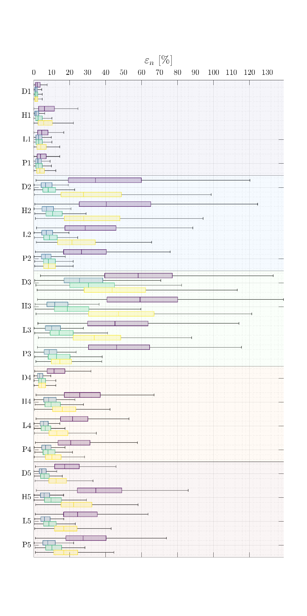
From Fig. 6, Fig. 7, and Fig. 8 global performance in terms of $\varepsilon_{n}$ are summarized for all cases considered. From these plots, it is possible to draw important considerations on the importance of labeling strategy, reference frame, and training method.

In Fig. 6 the box plot are organized from top-down in groups of 5 by macro-categories based on the labeling strategy and then in clusters of 4 based on the Image Processing method, ordered from top-down as Convolutional Extreme Learning Machine, Convolutional Neural Network, Hybrid Convolutional Extreme Learning Machine, and Hybrid Convolutional Extreme Learning Machine 3. It is possible to immediately appreciate that all the methods trained with the labeling strategy based on ( $\bm{\delta},\rho$ ) outperform all others considered. This is especially remarkable for the Convolutional Extreme Learning Machine method, which is performing similarly to the other Image Processing methods when considering this labeling strategy. On the other hand, in all other cases, Convolutional Extreme Learning Machine-based methods perform poorly. This is especially true when compared with the Convolutional Neural Network ones, which outperform all methods considered in all possible combinations. Focusing on the importance of the reference frame, it is observed that overall better performances are achieved when the labels are expressed in the $W$ reference frame than in the $AS$ one, while the choice of the coordinate system (cartesian or polar) seems to cause only minor differences.

An even more concise representation is visible in the semi-log plot of the mean $\varepsilon_{n}$ error clustered by body in Fig. 7. Once again it is possible to appreciate the much better performance achieved with the ( $\bm{\delta},\rho$ ) labeling strategy compared to the other ones for all bodies considered. In such a case, the performance of the Convolutional Extreme Learning Machine method is not so different than the one of the Convolutional Neural Network. While the former have a mean $\varepsilon_{n}$ of 2.58, 8.63, 5.60, 5.02 (respectively for 65803 Didymos, 65803 Didymos, 103P/Hartley, and 67P/Churyumov–Gerasimenko), the latter generates position estimates only 1.68, 4.11, 1.68, and 1.63 times better. Apart from 103P/Hartley, this means that only a very marginal performance gain is achieved with the use of a Convolutional Neural Network rather than a Convolutional Extreme Learning Machine. This does not hold when comparing Convolutional Extreme Learning Machine and Convolutional Neural Network performances for other labeling strategies, which show much wider gaps. From Fig. 7 it is also possible to observe a trend depending on the shape considered: simpler, regular shapes such as the one of Didymos (65803 Didymos) are better exploited for navigation than highly irregular ones such as Lutetia (21 Lutetia), 67P (67P/Churyumov–Gerasimenko), and Hartley (103P/Hartley).

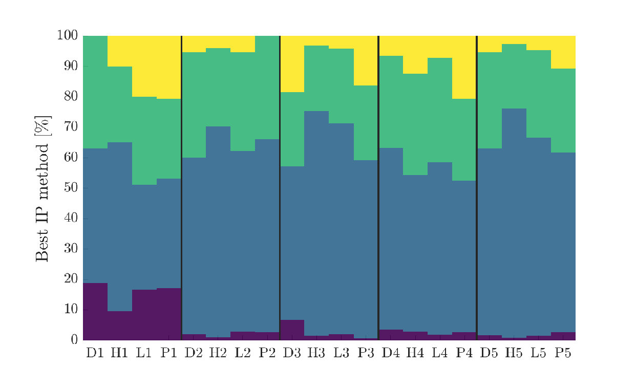
Finally, Fig. 8 reports in a stacked histogram plot the share for each dataset in which an Image Processing method performs better than all others considered. While the Convolutional Neural Network is always the best candidate, Hybrid Convolutional Extreme Learning Machine consistently scores as the second best method across all datasets considered. Moreover, the Convolutional Extreme Learning Machine is considered the best third option only in the case of the ( $\bm{\delta},\rho$ ) labeling strategy. This graphic representation is possible thanks to the fact that the geometric points considered across the test sets are the same.

Since it is observed that the labeling strategy based on ( $\bm{\delta},\rho$ ) works better than the others, the performance is further investigated in this case. In Fig. 9 the histograms of the $\varepsilon_{CoF}$ and $\varepsilon_{\rho}$ metrics in $\mathbb{S}_{2}$ space are illustrated. When considering 65803 Didymos, it is commented that the Convolutional Extreme Learning Machine shows a much larger mean error in $\varepsilon_{CoF}$ than the other methods while only a smaller variability both in terms of means and variance is observed in $\varepsilon_{\rho}$ . The fundamental failure mechanism for which the Convolutional Extreme Learning Machine method performs worse than the Convolutional Neural Network one with 65803 Didymos is thus represented by a larger mean error in the estimated Center of Figure coordinates. When considering 21 Lutetia and 67P/Churyumov–Gerasimenko, the difference between the histograms of the various methods is more subtle since only small variations in the mean and variance are observed across the different methods. On the other hand, when considering 103P/Hartley, it is possible to see that Convolutional Neural Network is much more accurate both in the Center of Figure and range estimates than all other methods. The hybrid Convolutional Extreme Learning Machine performs better in the range estimate (with similar variance than the Convolutional Neural Network) but does not perform at the same level as the Convolutional Neural Network in the Center of Figure estimate.

In Fig. 10 the error ellipses of the Center of Figure coordinate in $\mathbb{S}_{2}$ space are illustrated together with the error ellipse (dashed dark ellipse) that would have been obtained by not correcting the Center of Brightness with a data-driven scattering law implemented by the Image Processing. It is also observed that different than all other ellipses, the Convolutional Extreme Learning Machine ellipse with 65803 Didymos is not centered in the zero error point thus introducing a bias that is causing the larger mean error already observed in Fig. 9.

In Fig. 11 a representative case of the position error of the Convolutional Extreme Learning Machine in $CAM$ reference frame for the 21 Lutetia body is illustrated. It is possible to see that the position error is one order of magnitude higher in the boresight direction of the camera than on the other axis. This result is expected from optical-based navigation systems. This means that the error in the range estimate from the body is the major contributor to the positioning performances when using this labeling strategy.

Eventually, a visualization of a sample of $150$ images in $\mathbb{S}_{2}$ and the Center of Figure prediction by the different Image Processing methods is illustrated in Fig. 12.

4 Conclusions

In this work, Convolutional Extreme Learning Machines are investigated as a possible alternative to Convolutional Neural Networks for autonomous vision-based navigation systems around small bodies. This is done in an extensive analysis considering 4 different small body shapes and 5 different labeling strategies, for a total of 20 scenarios, each of which is examined with 4 different Image Processing methods, resulting in tens of thousands of different architectures explored.

It is demonstrated that the coupling between Image Processing method and labeling strategy plays a fundamental role to achieve the desired performance. In particular, the ( $\bm{\delta},\rho$ ) labeling strategy is found to be the best one. In this case, the navigation labels are given by two geometrical quantities which are estimated directly from the image, and a third, more difficult, label associated with the range from the body. The error on such a label is the one driving the error in the position estimate.

It is also noted that amongst the other labeling strategies, the ones adopting the $W$ reference frame perform better than those using the $AS$ one. This hints at the fact that in the former the estimated position relies on the correlation with global geometric properties of the body which are not dependent on the specific rotational state but are rather dependent on the illumination conditions. On the contrary, in the latter, the methods need to learn illumination invariant features that correlate to the specific rotational state of the body. This seems to be much harder to do, at least when $7500$ images are considered for training. Future work will be focused on changes in the method to allow larger datasets to be used. Irrespective of the reference frame, it is commented that the mapping from images to polar or cartesian coordinates seems to degrade the performance. In particular, while the ( $\bm{\delta},\rho$ ) and ( $\phi_{1}$ , $\phi_{2}$ , $\rho$ ) labeling strategies both share $\rho$ as a label, the latter performs considerably worse than the former. This may hint at a more difficult mapping from images into two angles in spherical coordinates than the mapping to projective quantities in the image plane, the latter correlating much easily and directly from image.

Although the Convolutional Neural Network outperform all other methods considered, the Convolutional Extreme Learning Machine seems a credible alternative, since it performs in the same order of magnitude as the Convolutional Neural Network method when considering the best labeling strategy.

It is also commented that the usage of Convolutional Extreme Learning Machine for exploration of the architecture space generated Convolutional Neural Network architectures that experienced robust training. This bootstrap training strategy could be deployed as a standard and efficient way to explore the global architecture space as suggested in [6]. Moreover, consistently with the findings in [6, 4, 5, 7], a preference is observed for orthogonalization of the weights and biases of the kernels, as it is possible to see from the best hyper-parameters $\bm{\Theta}$ in Tab. 4.

Future works will address the addition of dropout into the networks to generate uncertainty estimates, algorithmic design choices to adapt the Convolutional Extreme Learning Machine for small body images, larger datasets, and the usage of segmentation maps as input in place of grayscale images, the former representing easier input to work with.

Acknowledgments

The authors would like to acknowledge the funding received from the European Union’s Horizon 2020 research and innovation programme under the Marie Skłodowska-Curie grant agreement No 813644. A special thanks to Prof. Roberto Furfaro, whose seminar at the Deep-Space Astrodynamics Research & Technology Group on the application of Extreme Learning Machine theory in Physics Informed Neural Networks contributed to the main idea behind this paper.

References

Quadrelli et al. [2015] Quadrelli, M. B., Wood, L. J., Riedel, J. E., McHenry, M. C., Aung, M., Cangahuala, L. A., Volpe, R. A., Beauchamp, P. M., and Cutts, J. A., “Guidance, Navigation, and Control Technology Assessment for Future Planetary Science Missions,” Journal of Guidance, Control, and Dynamics, Vol. 38, No. 7, 2015, pp. 1165–1186. doi: 10.2514/1.g000525.
Szeliski [2022] Szeliski, R., Computer Vision, 2^nd ed., Springer International Publishing, 2022. doi: 10.1007/978-3-030-34372-9.
Huang et al. [2006] Huang, G.-B., Zhu, Q.-Y., and Siew, C.-K., “Extreme learning machine: Theory and applications,” Neurocomputing, Vol. 70, No. 1-3, 2006, pp. 489–501. doi: 10.1016/j.neucom.2005.12.126.
Huang [2014] Huang, G.-B., “An Insight into Extreme Learning Machines: Random Neurons, Random Features and Kernels,” Cognitive Computation, Vol. 6, No. 3, 2014, pp. 376–390. doi: 10.1007/s12559-014-9255-2.
Huang et al. [2015a] Huang, G., Huang, G.-B., Song, S., and You, K., “Trends in extreme learning machines: A review,” Neural Networks, Vol. 61, 2015a, pp. 32–48. doi: 10.1016/j.neunet.2014.10.001.
Saxe et al. [2011] Saxe, A. M., Koh, P. W., Chen, Z., Bhand, M., Suresh, B., and Ng, A. Y., “On Random Weights and Unsupervised Feature Learning,” Proceedings of the 28th International Conference on Machine Learning, ICML 2011, Bellevue, Washington, USA, June 28 - July 2, 2011, edited by L. Getoor and T. Scheffer, Omnipress, 2011, pp. 1089–1096. URL https://icml.cc/2011/papers/551_icmlpaper.pdf.
Huang et al. [2015b] Huang, G.-B., Bai, Z., Kasun, L. L. C., and Vong, C. M., “Local Receptive Fields Based Extreme Learning Machine,” IEEE Computational Intelligence Magazine, Vol. 10, No. 2, 2015b, pp. 18–29. doi: 10.1109/mci.2015.2405316.
Rodrigues et al. [2021] Rodrigues, I. R., da Silva Neto, S. R., Kelner, J., Sadok, D., and Endo, P. T., “Convolutional Extreme Learning Machines: A Systematic Review,” Informatics, Vol. 8, No. 2, 2021, p. 33. doi: 10.3390/informatics8020033.
Pugliatti M. et al. [2021] Pugliatti M., Franzese V., and Topputo F., “Data-Driven Image Processing for Onboard Optical Navigation Around a Binary Asteroid,” Journal of Spacecraft and Rockets, Vol. 59, 2021, pp. 943–959. doi: 10.2514/1.A35213.
Pugliatti and Maestrini [2022] Pugliatti, M., and Maestrini, M., “Small-Body Segmentation Based on Morphological Features with a U-Shaped Network Architecture,” Journal of Spacecraft and Rockets, 2022. Pre-print.
Otsu [1979] Otsu, N., “A Threshold Selection Method from Gray-Level Histograms,” IEEE Transactions on Systems, Man, and Cybernetics, Vol. 9, No. 1, 1979, pp. 62–66. doi: 10.1109/TSMC.1979.4310076.
Christian [2021] Christian, J. A., “A Tutorial on Horizon-Based Optical Navigation and Attitude Determination With Space Imaging Systems,” IEEE Access, Vol. 9, 2021, pp. 19819–19853. doi: 10.1109/ACCESS.2021.3051914.