Adaptive importance sampling based on fault tree analysis for piecewise deterministic Markov process

If there is no jump between time $s$ and time $s+h$, the mode $M_{s+h}$ of the PDMP remains constant and equal to $M_{s}$ and the position $X_{s+h}$ of the PDMP evolves in a deterministic way from $X_{s}$ as $\phi_{M_{s}}(X_{s},h)$ where $\phi_{m}$ is the solution of the differential equation $\dfrac{d\phi_{m}}{dh}=\bm{g}(\phi_{m},m)$, $\phi_{m}(x,h=0)=x$. Here $\bm{g}:\mathbb{R}^{d_{X}}\times\mathbb{M}\rightarrow\,\mathbb{R}^{d_{X}}$ is a Lipschitz function. The trajectory of the process $(X_{s+h},M_{s+h})$ is then of the form $\Phi_{(X_{s},M_{s})}(h)$ where the flow function $\Phi$ is defined by:

By denoting $E_{m}:=\left\{z^{\prime}=(x^{\prime},m^{\prime})\in E\ |\ m^{\prime}=m\right\}$ we can write $E=\bigcup_{m\in\mathbb{M}}E_{m}$. The boundary of the state space $E_{m}$ for $m\in\mathbb{M}$ is denoted by $\partial E_{m}$. When the position reaches the boundary of the state space following the flow $\Phi$, the PDMP jumps. Starting from a state $z=(x,m)\in E_{m}$ at time $s$ and assuming that no random jump takes place, the boundary $\partial E_{m}$ is reached at a deterministic time $t_{z}^{\partial}\in[0,+\infty]$:

with the convention $\inf\emptyset=+\infty$.

For each state $z\in E$, there is a random waiting time $T_{z}$ at the end of which the process jumps (if it is smaller than the deterministic jump time $t_{z}^{\partial}$). The jump intensity $\lambda$ is a function that associates to each state $z\in E$ a weight $\lambda(z)\in(0,+\infty)$. The larger $\lambda(z)$ is, the more likely it is that the PDMP jumps when it passes through state $z$. The distribution of $T_{z}$ depends on $\lambda$ through the following formula:

Given the jump time and the state $z^{-}$ from which the process jumps, the arrival state of the process after the jump is randomly chosen according to a Markovian transition kernel $\mathcal{K}(z^{-},\cdot)$. It is assumed for any $z^{-}$ that the transition kernel $\mathcal{K}(z^{-},\cdot)$ admits a probability density function $K\left(z^{-},\cdot\right)$ with respect to a reference measure $\nu_{z^{-}}$ on $\mathscr{B}(E)$ (where $\mathscr{B}(\cdot)$ indicates the Borelians of a set). So for any $B\in\mathscr{B}(E)$:

A fixed-time trajectory of a PDMP possesses a probability density function with respect to a dominant measure denoted by $\zeta$ which is a mixture of Lebesgue and Dirac measures. The definition of this dominant measure and the density of the PDMP trajectory can be found in Definition 3.2 and Theorem 3.3 of [16], respectively. Using our notations, the expression for this density is as follows. Let $\mathcal{Z}=\left(Z_{t}\right)_{t\in[0,t_{\max}]}$ be a PDMP trajectory and $n_{\mathcal{Z}}$ its number of jumps. We denote by $z_{0}$ the initial state of the trajectory, by $t_{0}$ the waiting time before the first jump, and for $k=1,\dots,n_{\mathcal{Z}}-1$ we denote by $z_{k}$ the state of the process after the $k$-th jump and by $t_{k}$ the waiting time between the $k$-th and the $(k+1)$-th jump. Finally let $t_{n_{\mathcal{Z}}}=t^{\partial}_{z_{n_{\mathcal{Z}}}}=t_{\max}-\sum_{k=0}^{n_{\mathcal{Z}}-1}t_{k}$. The probability density function of this trajectory can then be expressed as:

We consider the state space $E$ and the flow $\Phi$ of the PDMP fixed once and for all in this paper. A distribution $\pi_{\lambda,K}$ of a PDMP trajectory on $\mathcal{E}$ can thus be totally determined by the choice of the jump intensity $\lambda$ and the jump kernel density $K$.

In the case of industrial systems, the position of the PDMP contains the physical variables that determine the failure of the system and if necessary all the variables allowing the process to be Markovian such as the elapsed time. The physical variables evolve in time according to the flow $\Phi$ given by physical laws. The mode of the PDMP contains the status of each component (active, inactive, broken, etc.). The failure and repair rates of each component (which can depend on the value of the physical variables) determine the jump intensity $\lambda$ and the jump kernel density $K$ (see section 5 for a numerical example).

The system fails when the position reaches a critical region $\mathbb{X}_{D}$ determined by threshold values for the physical variables. The critical region $\mathbb{X}_{D}$ can only be reached in certain modes (the critical thresholds cannot be reached by the physical variables when all components are functioning, for example). Let $\mathbb{M}_{D}$ denote the set of modes $m$ such that the position can reach $\mathbb{X}_{D}$ by following the flow $\phi_{m}$ corresponding to the mode $m$. The set of states corresponding to a failed system is therefore $D=\mathbb{X}_{D}\times\mathbb{M}_{D}\subset E$. The set of faulty trajectories is written $\mathcal{D}\subset\mathcal{E}$ and corresponds to:

We denote by $\lambda_{0}$, $\mathcal{K}_{0}$ and $K_{0}$ the jump intensity, jump kernel and jump kernel density of the PDMP modeling the system whose failure probability we wish to estimate, and $\pi_{0}\equiv\pi_{\lambda_{0},K_{0}}$ the corresponding PDMP distribution. Our objective is to estimate the following probability:

Most of the computational cost for complex industrial systems comes from solving the differential equations that define the flow of the PDMP. We consider in the following that simulating several tens of uniform random variables and evaluating the density of a PDMP trajectory have a negligible cost compared to the computation of the flow between two jumps. This will guide the choice of our jump time simulation method and our optimization strategy for AIS (both are described in section 4). Note that, even if the flow appears in the formula of the density of a trajectory eq. 5, it does not have to be computed again since it was already evaluated to generate the trajectory.

We propose a redesigned version of the system presented in [18]. It is a simplification of the real operation of the storage pools of water for spent fuel from nuclear reactors. The water in the pool cools the fuel and provides protection from radiation. Conversely, the fuel heats the water in the pool, which will eventually boil, evaporate and allow the fuel to damage the structure and contaminate the outside environment. System failure is declared when the water level in the pool has reached a critical level. All the components of the system (shown in fig. 1) are designed to keep the water in the pool cold enough to prevent it from evaporating.

On this system the position of the PDMP corresponds to the water temperature and the water level in the pool; its mode is the combination of the status (active, inactive, broken) of the components. The domain $D$ is defined by all the states of $E$ in which the water temperature (first coordinate of the position) is $100^{\circ}\text{C}$ and the water level (second coordinate of the position) is lower or equal to the critical threshold. We notice that these positions are not accessible for the flow for all modes, for example if no component is broken. If on the other hand, all the generators $\texttt{G}_{0},\texttt{G}_{1},\texttt{G}_{2}$ and $\texttt{G}_{3}$ are and remain broken for example, then the flow reaches one of these positions in finite time. A more formal description of the modes allowing the flow to bring the process into $D$ is given in section 2. This description will turn out to be important to build a good estimator of the failure probability. The system data allowing to compute the flow, and the different failure and repair rates of each component allowing to build the jump intensities and kernels are given in section 5.

It is well known that CMC methods are quite inefficient in this case because an overwhelming majority of realizations will not produce any failure. A CMC estimator of $P$ from an i.i.d sample $\mathcal{Z}_{1},\dots,\mathcal{Z}_{N}\sim\pi_{0}$ is given by:

An accurate CMC estimator of $P$ (say with a coefficient of variation of 0.1) requires about $\nicefrac{{100}}{{P}}$ realizations. Each realization implies to simulate a PDMP trajectory which is very expensive especially for large industrial systems (as previously mentioned, the deterministic parts of the trajectory correspond to complex physical phenomena and result from the resolution of expensive computer codes). It is therefore unthinkable to simulate several tens of millions of trajectories to estimate the probability of system failure.

Introduced in 1951 by Kahn and Harris [31], importance sampling is used to estimate the expectation of a random quantity under an arbitrary distribution. In the context of rare event simulation, this method allows to estimate the probability $P$ of the rare event using an instrumental distribution $q$ whose support is included in the support of the original distribution $\pi_{0}$ and that realizes the event more frequently than it. See [9] for a rare event perspective of IS, [56] for a recent review of IS methods in reliability assessment and [29] for recent advances in IS for more general purpose. From the formula

we can deduce the form of the importance sampling estimator of $P$ with an i.i.d sample $\mathcal{Z}_{1},\dots,\mathcal{Z}_{N}\sim q$:

The variance of $\widehat{P}_{N}^{\text{IS}}$ strongly depends on the choice of $q$. The optimal distribution $q_{\text{opt}}:\mathcal{Z}\mapsto\frac{1}{P}\mathds{1}_{\mathcal{Z}\in\mathcal{D}}\,\pi_{0}(\mathcal{Z})$ produces a zero variance IS estimator. Although inaccessible in practice, this form guides us on the choice of the instrumental density to use. We also know from [16] that the process of distribution $q_{\text{opt}}$ is a PDMP with the same state space and with the same deterministic flow as the original PDMP of distribution $\pi_{0}$.

The optimal jump intensity $\lambda_{\text{opt}}$ and optimal jump kernel density $K_{\text{opt}}$ given in eq. 12 can be expressed in terms of the committor function of the process $U_{\text{opt}}$. It is defined here as follows for any states $z^{-},z\in E$ by:

$U_{\text{opt}}$ represents the probability of reaching $\mathcal{D}$ knowing the current state of the trajectory and $U_{\text{opt}}^{-}$ represents the same quantity with the additional assumption that the process jumps immediately. Theorems 4.3 and 4.4 of [16] give us the following result:

Remark: understanding these equations gives a good intuition of the behavior of the optimal process. If from a given state $z^{-}\in E$:

1. 1.

   the process is $k$ times more likely to reach $D$ before the end of the simulation by jumping now than by not jumping, then the optimal intensity $\lambda_{\text{opt}}$ must be $k$ times larger than the nominal intensity $\lambda_{0}$,

2. 2.

   and if the process is $k$ times more likely to reach $D$ before the end of the simulation by jumping to state $z$ than by jumping randomly according to $\mathcal{K}$, then the value of the optimal jump kernel density $K_{\text{opt}}$ between $z^{-}$ and $z$ must be $k$ times larger than that of the nominal jump kernel density $K_{0}$.

The optimal distribution $q_{\text{opt}}$ is thus completely characterized by the original distribution $\pi_{0}$ and by the committor function $U_{\text{opt}}$.

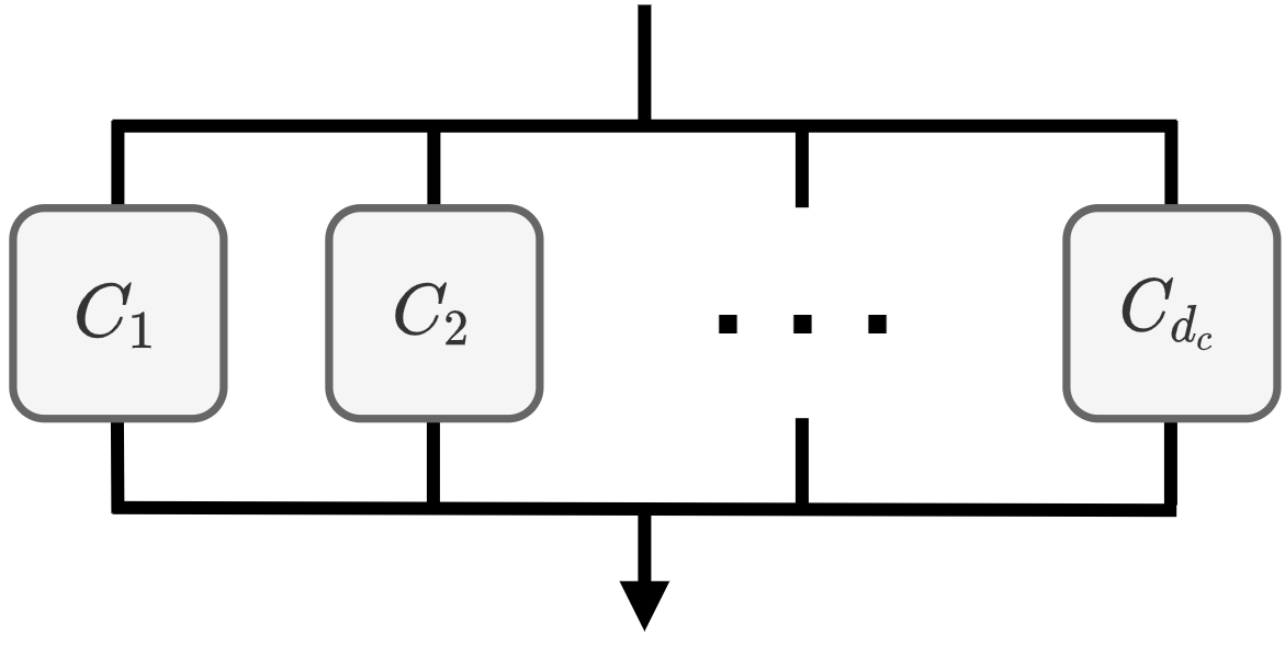
Here are two extreme examples of industrial systems to keep in mind for the following. A series system is a configuration of components in which the failure of any one component is sufficient to cause system failure (see Figure 3). A parallel system is a configuration of components in which the failure of all components is necessary to cause system failure (see Figure 3). A series system has only one MPS and a parallel system has $d_{\bm{c}}$ MPS. In contrast, a series system has $d_{\bm{c}}$ MCS and a parallel system has only one MCS.

The test case described in section 1.1 can be represented as a series/parallel diagram (see Figure 4) facilitating its decomposition into MPS and MCS. The MPS correspond to all vertical combinations and the MCS to all horizontal combinations.

Let $d_{\bm{c}}\in\mathbb{N}^{*}$ and $\bm{c}=(c_{1},\dots,c_{d_{\bm{c}}})\in\{0,1\}^{d_{\bm{c}}}$, we note $\llbracket 1,d_{\bm{c}}\rrbracket=\{1,\dots,d_{\bm{c}}\}$ and for any $I\subset\llbracket 1,d_{\bm{c}}\rrbracket$:

Let $\bm{c}^{\prime}=(c_{1}^{\prime},\dots,c_{d_{\bm{c}}}^{\prime})\in\{0,1\}^{d_{\bm{c}}}$, we write $\bm{c}\leq\bm{c}^{\prime}$ if and only if $c_{j}\leq c_{j}^{\prime}$ for all $j\in\llbracket 1,d_{\bm{c}}\rrbracket$. Let $\varphi$ be a Boolean function, i.e from $\{0,1\}^{d_{\bm{c}}}$ to $\{0,1\}$. The function $\varphi$ is non-decreasing if and only if $\varphi(\bm{c})\leq\varphi(\bm{c}^{\prime})\Longleftrightarrow\bm{c}\leq\bm{c}^{\prime}$ for all $\bm{c},\bm{c}^{\prime}\in\{0,1\}^{d_{\bm{c}}}$. Combining Theorem 1.14 and Theorem 1.21 from [21], we obtain the following decomposition:

If a system has $d_{\bm{c}}$ components we now consider that the PDMP mode $m\in\mathbb{M}$ can be converted into a multidimensional binary variable $b_{m}=(c_{1},\dots,c_{d_{\bm{c}}})\in\{0,1\}^{d_{\bm{c}}}$ where for $j\in\llbracket 1,d_{\bm{c}}\rrbracket$, $c_{j}$ is 0 if the $j$-th component is broken and 1 otherwise.

We assume from now that the system is coherent, so we can apply theorem 2 to its structure function $\varphi$. There are then $d_{\text{MPS}}$ sets of components $I_{1},\dots,I_{d_{\text{MPS}}}\subset\llbracket 1,d_{\bm{c}}\rrbracket$ such that none of them is contained in another and such that the operation of all the components of a set causes the operation of the system independently of the status of the components in the other sets. These sets are the unique minimal paths sets of the system. By switching to the complementary with $\overline{c}=1-c$ for any $c\in\{0,1\}$, we can notice that:

Therefore the minimal paths sets can be alternatively defined such that the failure of at least one component in each set causes the system failure.

Let us first note that since $\varphi$ is a non-decreasing Boolean function, the function $b_{m}\mapsto\overline{\varphi\left(\overline{b_{m}}\right)}$ is also non-decreasing (it is called the dual function of $\varphi$). Indeed: let $b_{m}\leq b^{\prime}_{m}\in\{0,1\}^{d_{\bm{c}}}$, we have $\overline{b_{m}}\geq\overline{b^{\prime}_{m}}$ so $\varphi\left(\overline{b_{m}}\right)\geq\varphi\left(\overline{b^{\prime}_{m}}\right)$ and finally $\overline{\varphi\left(\overline{b_{m}}\right)}\leq\overline{\varphi\left(\overline{b^{\prime}_{m}}\right)}$. We can therefore apply theorem 2 to it and get a set of $d_{\text{MCS}}$ lists of indices $J_{1},\dots,J_{d_{\text{MCS}}}\subset\llbracket 1,d_{\bm{c}}\rrbracket$ with $J_{i}\not\subset J_{i^{\prime}}$ for any $i,i^{\prime}\in\llbracket 1,d_{\text{MCS}}\rrbracket$ with $i\neq i^{\prime}$ such that:

These $d_{\text{MCS}}$ sets of components $J_{1},\dots,J_{d_{\text{MCS}}}$ are the unique minimal cuts sets of the system. If all the components of a MCS are broken then this causes (from the static point of view) the system failure. And again by switching to the complementary, if at least one component per MCS works, the system failure is prevented:

The authors of [16] have successfully tested this one-dimensional approach on a parallel system with 3 components and a single failing mode (when all components are broken). It is reasonable to think that the number of components is not the core of the problem for parallel systems and that our $d_{\bm{c}}$-dimensional extension adds enough flexibility if needed for very large parallel systems. On the other hand, there is concern that this approach is too naive to approximate $U_{\text{opt}}$ in the case of systems with both many components and multiple failing modes. Typical failures do not involve a large number of components but a small number of key components. Using $U_{\bm{\theta}}^{(\text{BC})}$ produces trajectories where blindly selected components will break. With small $\bm{\theta}$ it may not break the right components, and with large $\bm{\theta}$ it may break too many and produce implausible trajectories (with a low likelihood ratio in the IS estimator eq. 10). We must therefore take into account the role played by each component within the system.

A MPS is said damaged when at least one of its components is broken. It is necessary that all minimal paths sets are damaged to reach system failure. For $\bm{\theta}=\left(\theta_{1},\dots,\theta_{d_{\text{MPS}}}\right)\in\mathbb{R}^{d_{\text{MPS}}}$, we recycle the idea expressed in eq. 19 but with this time an increasing function in $\beta^{(\text{MPS})}(z)$ the number of damaged MPS in state $z$:

The process simulated from $U_{\bm{\theta}}^{\text{(MPS)}}$ therefore prioritizes the failure of components involved in a large number of still undamaged MPS (and conversely will prioritize preventing the repair of components involved in a large number of already damaged MPS).

The MPS-IF does not consider the number of broken components per MPS but only the presence of at least one broken component. This means that the form $U_{\bm{\theta}}^{\text{(MPS)}}$ does not look for breaking two components in a single MPS if they are not present in other MPS. Yet, even if this second broken component is not necessary to achieve system failure, it prevents the system from being safe in the case when the first component is repaired. Describing the functioning of the system with MCS rather than MPS leads us to a more flexible parametric family since this time we have to look at the proportion of broken components in each MCS.

For any state $z\in E$ and any $i\in\llbracket 1,d_{\text{MCS}}\rrbracket$, we define $\beta^{(\text{MCS})}_{i}(z)$ the proportion of broken components in the $i$-th MCS when the process is in the state $z$. We rank these proportions in descending order and we also define $\beta^{(\text{MCS})}_{(i)}(z)$ the $i$-th largest proportion of broken components among all MCS in the state $z$:

Here again, the process simulated from $U_{\bm{\theta}}^{\text{(MCS)}}$ prioritizes the failure of components involved in a large number of MCS or in MCS of small size (to bring the proportions of broken components closer to 1 more quickly).

A key point for the success of the method is to get a flexible but reasonably sized family. One way to reduce the dimension of $\bm{\theta}$ is to impose the equality of some groups of coordinates (by ordered packets). For example, to get a vector $\bm{\theta}\in\mathbb{R}^{d_{\bm{\theta}}}$ from $\widetilde{\bm{\theta}}\in\mathbb{R}^{d_{\widetilde{\bm{\theta}}}}$ with $d_{\bm{\theta}}=k\times d_{\widetilde{\bm{\theta}}}$ we impose $\theta_{i}=\widetilde{\theta}_{\lfloor\frac{i-1}{k}\rfloor+1}$ for $i\in\llbracket 1,d_{\bm{\theta}}\rrbracket$. This is why by choosing $\mathds{1}_{\beta\geq i}$ in eq. 19 and eq. 20 instead of simply $\mathds{1}_{\beta=i}$, and $\beta^{(\text{MCS})}_{(i)}$ instead of $\beta^{(\text{MCS})}_{i}$ in eq. 21, we keep a consistent (and increasing in each coordinate) $U_{\bm{\theta}}$ even with $d_{\widetilde{\bm{\theta}}}=1$.

The function $\bm{\theta}\mapsto\mathbb{E}_{\pi_{0}}\left[-\mathds{1}_{\mathcal{Z}\in\mathcal{D}}\,\log\left(q_{\bm{\theta}}\left(\mathcal{Z}\right)\right)\right]$ is estimated by importance sampling under an initial instrumental distribution $q_{\bm{\theta}^{(\bm{1})}}$, we determine $\bm{\theta}^{(2)}$ which minimizes this estimate and we repeat the scheme. To save the simulation budget, we reuse at each iteration all the trajectories already drawn to perform the minimization step. Similarly, all the trajectories generated during the algorithm are recycled to produce the final estimator of $P$. To summarize, at iteration $\ell\in\mathbb{N}^{*}$:

1. 1.

   Simulation phase. Generate $n_{\ell}$ trajectories $\mathcal{Z}_{1}^{(\ell)},\dots,\mathcal{Z}_{n_{\ell}}^{(\ell)}\,\overset{\text{i.i.d.}}{\sim}\,q_{\bm{\theta}^{(\ell)}}$.

2. 2.

   Optimization phase. Update the parameter of the instrumental distribution with the $\ell$ last samples drawn $\left(\mathcal{Z}_{k}^{(1)}\right)_{k=1}^{n_{1}},\dots,\left(\mathcal{Z}_{k}^{(\ell)}\right)_{k=1}^{n_{\ell}}$:

   $$\bm{\theta}^{(\ell+1)}=\underset{\bm{\theta}\in\Theta}{\arg\min}\left\{-\sum_{r=1}^{\ell}\sum_{k=1}^{n_{r}}\mathds{1}_{\mathcal{Z}_{k}^{(r)}\in\mathcal{D}}\frac{\pi_{0}\big(\mathcal{Z}_{k}^{(r)}\big)}{q_{\bm{\theta}^{(r)}}\big(\mathcal{Z}_{k}^{(r)}\big)}\log\left[q_{\bm{\theta}}\big(\mathcal{Z}_{k}^{(r)}\big)\right]\right\}.$$

   (23)

Estimation phase at the final iteration $L$ (with $N_{L}=\sum_{\ell=1}^{L}n_{\ell}$ the total budget), we reuse all past samples to get the final estimator of $P$ :

References

- [1] A. Abate, H. Blom, M. Bouissou, N. Cauchi, H. Chraibi, J. Delicaris, S. Haesaert, A. Hartmanns, M. Khaled, A. Lavaei, et al., Arch-comp21 category report: Stochastic models, in 8th International Workshop on Applied Verification of Continuous and Hybrid Systems, ARCH 2021, EasyChair, 2021, pp. 55–89.
- [2] R. Arismendi, A. Barros, and A. Grall, Piecewise deterministic markov process for condition-based maintenance models — application to critical infrastructures with discrete-state deterioration, Reliability Engineering & System Safety, 212 (2021), p. 107540.
- [3] R. Azaïs, J.-B. Bardet, A. Génadot, N. Krell, and P.-A. Zitt, Piecewise deterministic Markov process — recent results, ESAIM: Proceedings, 44 (2014), pp. 276–290.
- [4] J. Bierkens, P. Fearnhead, and G. Roberts, The zig-zag process and super-efficient sampling for Bayesian analysis of big data, The Annals of Statistics, 47 (2019), pp. 1288–1320.
- [5] H. A. Blom, H. Ma, and G. B. Bakker, Interacting particle system-based estimation of reach probability for a generalized stochastic hybrid system, IFAC-PapersOnLine, 51 (2018), pp. 79–84.
- [6] A. Bouchard-Côté, S. J. Vollmer, and A. Doucet, The bouncy particle sampler: A nonreversible rejection-free Markov chain Monte Carlo method, Journal of the American Statistical Association, 113 (2018), pp. 855–867.
- [7] M. Bouissou, H. Elmqvist, M. Otter, and A. Benveniste, Efficient Monte Carlo simulation of stochastic hybrid systems, in The 10th International Modelica Conference 2014, 2014.
- [8] C.-E. Bréhier, M. Gazeau, L. Goudenege, T. Lelièvre, and M. Rousset, Unbiasedness of some generalized adaptive multilevel splitting algorithms, Ann. Appl. Prob., 26 (2016), pp. 3559–3601.
- [9] J. A. Bucklew, Introduction to rare event simulation, Springer, New York, 2004.
- [10] C. E. Budde and M. Stoelinga, Automated rare event simulation for fault tree analysis via minimal cut sets, in International Conference on Measurement, Modelling and Evaluation of Computing Systems, Springer, 2020, pp. 259–277.
- [11] M. F. Bugallo, V. Elvira, L. Martino, D. Luengo, J. Miguez, and P. M. Djuric, Adaptive importance sampling: The past, the present, and the future, IEEE Signal Processing Magazine, 34 (2017), pp. 60–79.
- [12] M.-L. Bujorianu and J. Lygeros, General stochastic hybrid systems: Modelling and optimal control, in 2004 43rd IEEE Conference on Decision and Control (CDC)(IEEE Cat. No. 04CH37601), vol. 2, IEEE, 2004, pp. 1872–1877.
- [13] M. Čepin, Assessment of power system reliability: methods and applications, Springer Science & Business Media, 2011.
- [14] F. Cérou and A. Guyader, Adaptive multilevel splitting for rare event analysis, Stochastic Analysis and Applications, 25 (2007), pp. 417–443.
- [15] F. Cérou, A. Guyader, and M. Rousset, Adaptive multilevel splitting: Historical perspective and recent results, Chaos: An Interdisciplinary Journal of Nonlinear Science, 29 (2019), p. 043108.
- [16] H. Chraibi, A. Dutfoy, T. Galtier, and J. Garnier, On the optimal importance process for piecewise deterministic markov process, ESAIM: Probability and Statistics, 23 (2019), pp. 893–921.
- [17] H. Chraibi, A. Dutfoy, T. Galtier, and J. Garnier, Optimal potential functions for the interacting particle system method, Monte Carlo Methods and Applications, 27 (2021), pp. 137–152.
- [18] H. Chraibi, J. C. Houdebine, and A. Sibler, PyCATSHOO: Toward a new platform dedicated to dynamic reliability assessments of hybrid systems, in 13th International Conference on Probabilistic Safety Assessment and Management (PSAM 13), 2016.
- [19] J.-M. Cornuet, J.-M. Marin, A. Mira, and C. P. Robert, Adaptive multiple importance sampling, Scandinavian Journal of Statistics, 39 (2012), pp. 798–812.
- [20] O. L. Costa and F. Dufour, Stability and ergodicity of piecewise deterministic markov processes, SIAM Journal on Control and Optimization, 47 (2008), pp. 1053–1077.
- [21] Y. Crama and P. L. Hammer, Boolean functions: Theory, algorithms, and applications, Cambridge University Press, Cambridge, 2011.
- [22] Y.-H. Dai, Convergence properties of the BFGS algoritm, SIAM Journal on Optimization, 13 (2002), pp. 693–701.
- [23] M. H. A. Davis, Piecewise-Deterministic Markov Processes: A General Class of Non-Diffusion Stochastic Models, Journal of the Royal Statistical Society. Series B (Methodological), 46 (1984), pp. 353–388.
- [24] P.-T. De Boer, D. P. Kroese, S. Mannor, and R. Y. Rubinstein, A tutorial on the cross-entropy method, Annals of Operations Research, 134 (2005), pp. 19–67.
- [25] P. Del Moral and J. Garnier, Genealogical particle analysis of rare events, Ann. Appl. Prob., 15 (2005), pp. 2496–2534.
- [26] L. Desgeorges, P.-Y. Piriou, T. Lemattre, and H. Chraibi, Formalism and semantics of pycatshoo: A simulator of distributed stochastic hybrid automata, Reliability Engineering & System Safety, 208 (2021), p. 107384.
- [27] M. El Masri, J. Morio, and F. Simatos, Improvement of the cross-entropy method in high dimension for failure probability estimation through a one-dimensional projection without gradient estimation, Reliability Engineering & System Safety, 216 (2021), p. 107991.
- [28] M. ElMasri, J. Morio, and F. Simatos, Optimal projection to improve parametric importance sampling in high dimension, arXiv:2107.06091, (2021).
- [29] V. Elvira and L. Martino, Advances in importance sampling, Wiley StatsRef: Statistics Reference Online, (2021), pp. 1–14.
- [30] T. Galtier, Accelerated Monte-Carlo methods for piecewise deterministic Markov processes for a faster reliability assessment of power generation systems within the PyCATSHOO toolbox, PhD thesis, Université de Paris, 2019.
- [31] H. Kahn and T. E. Harris, Estimation of particle transmission by random sampling, National Bureau of Standards applied mathematics series, 12 (1951), pp. 27–30.
- [32] Y. Khoo, J. Lu, and L. Ying, Solving for high-dimensional committor functions using artificial neural networks, Research in the Mathematical Sciences, 6 (2019), pp. 1–13.
- [33] J. Krystul and H. A. Blom, Sequential Monte Carlo simulation of rare event probability in stochastic hybrid systems, IFAC Proceedings Volumes, 38 (2005), pp. 176–181.
- [34] A. Lasota, M. C. Mackey, and J. Tyrcha, The statistical dynamics of recurrent biological events, Journal of Mathematical Biology, 30 (1992), pp. 775–800.
- [35] W.-S. Lee, D. L. Grosh, F. A. Tillman, and C. H. Lie, Fault tree analysis, methods, and applications – a review, IEEE transactions on reliability, 34 (1985), pp. 194–203.
- [36] V. Lemaire, M. Thieullen, and N. Thomas, Exact simulation of the jump times of a class of piecewise deterministic markov processes, Journal of Scientific Computing, 75 (2018), pp. 1776–1807.
- [37] V. Lemaire, M. Thieullen, and N. Thomas, Thinning and multilevel Monte Carlo methods for piecewise deterministic (markov) processes with an application to a stochastic Morris–Lecar model, Advances in Applied Probability, 52 (2020), pp. 138–172.
- [38] P. W. Lewis and G. S. Shedler, Simulation of nonhomogeneous Poisson processes by thinning, Naval research logistics quarterly, 26 (1979), pp. 403–413.
- [39] Q. Li, B. Lin, and W. Ren, Computing committor functions for the study of rare events using deep learning, The Journal of Chemical Physics, 151 (2019), p. 054112.
- [40] H. Louvin, E. Dumonteil, T. Lelièvre, M. Rousset, and C. M. Diop, Adaptive multilevel splitting for monte carlo particle transport, in EPJ Web of Conferences, vol. 153, EDP Sciences, 2017, p. 06006.
- [41] D. Lucente, S. Duffner, C. Herbert, J. Rolland, and F. Bouchet, Machine learning of committor functions for predicting high impact climate events, arXiv:1910.11736, (2019).
- [42] J.-M. Marin, P. Pudlo, and M. Sedki, Consistency of adaptive importance sampling and recycling schemes, Bernoulli, 25 (2019), pp. 1977–1998.
- [43] R. T. McGibbon, B. E. Husic, and V. S. Pande, Identification of simple reaction coordinates from complex dynamics, The Journal of Chemical Physics, 146 (2017), p. 044109.
- [44] P. Metzner, C. Schütte, and E. Vanden-Eijnden, Transition path theory for markov jump processes, Multiscale Modeling & Simulation, 7 (2009), pp. 1192–1219.
- [45] G. Pola, M.-L. Bujorianu, J. Lygeros, and M. D. Di Benedetto, Stochastic hybrid models: An overview, IFAC Proceedings Volumes, 36 (2003), pp. 45–50.
- [46] F. Portier and B. Delyon, Asymptotic optimality of adaptive importance sampling, Advances in Neural Information Processing Systems, 31 (2018).
- [47] A. Rauzy, New algorithms for fault trees analysis, Reliability Engineering & System Safety, 40 (1993), pp. 203–211.
- [48] S. Razavi, A. Jakeman, A. Saltelli, C. Prieur, B. Iooss, E. Borgonovo, E. Plischke, S. L. Piano, T. Iwanaga, W. Becker, et al., The future of sensitivity analysis: an essential discipline for systems modeling and policy support, Environmental Modelling & Software, 137 (2021), p. 104954.
- [49] M. G. Riedler, Almost sure convergence of numerical approximations for piecewise deterministic markov processes, Journal of Computational and Applied Mathematics, 239 (2013), pp. 50–71.
- [50] G. Rubino and B. Tuffin, Rare event simulation using Monte Carlo methods, Wiley, 2009.
- [51] R. Y. Rubinstein and P. W. Glynn, How to deal with the curse of dimensionality of likelihood ratios in Monte Carlo simulation, Stochastic Models, 25 (2009), pp. 547–568.
- [52] R. Rudnicki and M. Tyran-Kamińska, Piecewise deterministic markov processes in biological models, in Semigroups of operators-theory and applications, Springer, 2015, pp. 235–255.
- [53] E. Ruijters and M. Stoelinga, Fault tree analysis: A survey of the state-of-the-art in modeling, analysis and tools, Computer Science Review, 15 (2015), pp. 29–62.
- [54] P. Rusnak, E. Zaitseva, F. Coolen, M. Kvassay, and V. Levashenko, Logic Differential Calculus for Reliability Analysis Based on Survival Signature, IEEE Transactions on Dependable and Secure Computing, (2022).
- [55] B. d. Saporta, F. Dufour, and H. Zhang, Numerical methods for simulation and optimization of piecewise deterministic Markov processes: application to reliability, Mathematics and statistics series, ISTE, 2016.
- [56] A. Tabandeh, G. Jia, and P. Gardoni, A review and assessment of importance sampling methods for reliability analysis, Structural Safety, 97 (2022), p. 102216.
- [57] P. Turati, N. Pedroni, and E. Zio, Advanced restart method for the estimation of the probability of failure of highly reliable hybrid dynamic systems, Reliability Engineering & System Safety, 154 (2016), pp. 117–126.
- [58] F. Uribe, I. Papaioannou, Y. M. Marzouk, and D. Straub, Cross-entropy-based importance sampling with failure-informed dimension reduction for rare event simulation, SIAM/ASA Journal on Uncertainty Quantification, 9 (2021), pp. 818–847.
- [59] P. Vanetti, A. Bouchard-Côté, G. Deligiannidis, and A. Doucet, Piecewise-deterministic Markov Chain Monte Carlo, arXiv:1707.05296, (2017).
- [60] R. Veltz, A new twist for the simulation of hybrid systems using the true jump method, arXiv:1504.06873, (2015).
- [61] P. Virtanen, R. Gommers, T. E. Oliphant, M. Haberland, T. Reddy, D. Cournapeau, E. Burovski, P. Peterson, W. Weckesser, J. Bright, et al., Scipy 1.0: fundamental algorithms for scientific computing in python, Nature methods, 17 (2020), pp. 261–272.
- [62] Z. Wang and J. Song, Cross-entropy-based adaptive importance sampling using von mises-fisher mixture for high dimensional reliability analysis, Structural Safety, 59 (2016), pp. 42–52.
- [63] P. Zuliani, C. Baier, and E. M. Clarke, Rare-event verification for stochastic hybrid systems, in Proceedings of the 15th ACM international conference on Hybrid Systems: Computation and Control, 2012, pp. 217–226.
Appendix A Appendix
A.1 Proof of theorem 7
The results come directly from showing that we verify the hypotheses of Theorems 2 and 3 from [46]. We know by 5 and 6 that is compact and that we have if . Moreover, for any the continuity of the application implies the continuity of for any . To obtain the convergence of the sequence , it remains to show that :