NeRFPlayer: A Streamable Dynamic Scene Representation with
Decomposed Neural Radiance Fields
Abstract
Visually exploring in a real-world 4D spatiotemporal space freely in VR has been a long-term quest. The task is especially appealing when only a few or even single RGB cameras are used for capturing the dynamic scene. To this end, we present an efficient framework capable of fast reconstruction, compact modeling, and streamable rendering. First, we propose to decompose the 4D spatiotemporal space according to temporal characteristics. Points in the 4D space are associated with probabilities of belonging to three categories: static, deforming, and new areas. Each area is represented and regularized by a separate neural field. Second, we propose a hybrid representations based feature streaming scheme for efficiently modeling the neural fields. Our approach, coined NeRFPlayer, is evaluated on dynamic scenes captured by single hand-held cameras and multi-camera arrays, achieving comparable or superior rendering performance in terms of quality and speed comparable to recent state-of-the-art methods, achieving reconstruction in 10 seconds per frame and interactive rendering.
![[Uncaptioned image]](2210.15947v2/teaser.png)
![[Uncaptioned image]](2210.15947v2/fig/guigif/flames0.jpg)
![[Uncaptioned image]](2210.15947v2/fig/guigif/chicken0.jpg) (a) Inputs
(b) Real-time rendering
(c) Low bitrate streaming
(a) Inputs
(b) Real-time rendering
(c) Low bitrate streaming
![[Uncaptioned image]](2210.15947v2/fig/guigif/flames1.jpg)
![[Uncaptioned image]](2210.15947v2/fig/guigif/chicken1.jpg) (a) Inputs
(b) Real-time rendering
(c) Low bitrate streaming
(a) Inputs
(b) Real-time rendering
(c) Low bitrate streaming
![[Uncaptioned image]](2210.15947v2/fig/guigif/flames2.jpg)
![[Uncaptioned image]](2210.15947v2/fig/guigif/chicken2.jpg) (a) Inputs
(b) Real-time rendering
(c) Low bitrate streaming
(a) Inputs
(b) Real-time rendering
(c) Low bitrate streaming
![[Uncaptioned image]](2210.15947v2/fig/guigif/flames3.jpg)
![[Uncaptioned image]](2210.15947v2/fig/guigif/chicken3.jpg) (a) Inputs
(b) Real-time rendering
(c) Low bitrate streaming
(a) Inputs
(b) Real-time rendering
(c) Low bitrate streaming
![[Uncaptioned image]](2210.15947v2/fig/guigif/flames4.jpg)
![[Uncaptioned image]](2210.15947v2/fig/guigif/chicken4.jpg) (a) Inputs
(b) Real-time rendering
(c) Low bitrate streaming
(a) Inputs
(b) Real-time rendering
(c) Low bitrate streaming
![[Uncaptioned image]](2210.15947v2/fig/guigif/flames5.jpg)
![[Uncaptioned image]](2210.15947v2/fig/guigif/chicken5.jpg) (a) Inputs
(b) Real-time rendering
(c) Low bitrate streaming
(a) Inputs
(b) Real-time rendering
(c) Low bitrate streaming
![[Uncaptioned image]](2210.15947v2/fig/guigif/flames6.jpg)
![[Uncaptioned image]](2210.15947v2/fig/guigif/chicken6.jpg) (a) Inputs
(b) Real-time rendering
(c) Low bitrate streaming
(a) Inputs
(b) Real-time rendering
(c) Low bitrate streaming
![[Uncaptioned image]](2210.15947v2/fig/guigif/flames7.jpg)
![[Uncaptioned image]](2210.15947v2/fig/guigif/chicken7.jpg) (a) Inputs
(b) Real-time rendering
(c) Low bitrate streaming
(a) Inputs
(b) Real-time rendering
(c) Low bitrate streaming
![[Uncaptioned image]](2210.15947v2/fig/guigif/flames8.jpg)
![[Uncaptioned image]](2210.15947v2/fig/guigif/chicken8.jpg) (a) Inputs
(b) Real-time rendering
(c) Low bitrate streaming
(a) Inputs
(b) Real-time rendering
(c) Low bitrate streaming
1 Introduction
Representing scenes as Neural Radiance Fields (NeRF) has brought a series of breakthroughs in 3D reconstruction and analysis xie2021neural; mildenhall2020nerf. High-fidelity real-time rendering of real-world scenes now can be obtained after a few seconds of training yu_and_fridovichkeil2021plenoxels; instantngp. The rendering system only requires a few real-world RGB images mildenhall2021rawnerf, but can well model scenes as small as a cell liu2022recovery and as large as a city tancik2022blocknerf or even a black hole levis2022gravitationally.
Despite NeRF’s success in static scenes, extending it to handle dynamic scenes remains challenging. Introducing an extra time dimension to NeRF’s 5D representation (3D location and 2D viewing direction ) is non-trivial for the following two reasons. First, the supervisory signal for a spatiotemporal point is sparser than a static point . Multi-view images of static scenes are easy to access as we can move the camera around, but an extra view in dynamic scenes requires an extra recording camera, leading to sparse input views. Second, the appearance and geometry frequency of the scene are different along the spatial axis and temporal axis. The content usually changes a lot when moving from one location to another location, but the background scene is unlikely to completely change from one timestamp to another. An inappropriate frequency modeling for the time dimension results in poor temporal interpolation performance.
A lot of progress has been made in addressing the aforementioned two challenges. Existing solutions include adopting motion models for matching the points (e.g., pumarola2020dnerf; nerfies; Tretschk_2021_ICCV; park2021hypernerf; liu2022devrf; fang2022fast) and leveraging data-driven priors like depth and optical flow (e.g., wang2021neural; nsff; xian2020space; du2021nerflow). Different from existing works, we are motivated by the observation that in dynamic scenes different spatial areas have different temporal characteristics. We assume that there are three kinds of temporal patterns in a dynamic scene (Figs. 2 and 3): static, deforming, and new areas. We thus propose to decompose the dynamic scene into these categories, which is achieved by a decomposition field that predicts the point-wise probabilities of being static, deforming, and new. The decomposition field is self-supervised and regularized by a manually assigned global parsimony regularization (e.g., suppressing the global probabilities of being new).
The proposed decomposition can address both of the aforementioned challenges. First, different temporal regularizations are introduced for each decomposed area, thus alleviating the ambiguity in reconstruction from sparse observations. For instance, the static area decomposition simplifies the dynamic modeling to a static scene modeling problem. The deforming areas enforce the foreground object to be consistent in the dynamic scene. Second, the scene is split into different areas according to their temporal characteristics, thus resulting in consistent frequency in the time dimension in each of the areas.
In response to the discrepancy between spatial and temporal frequency, we further decouple spatial and temporal dimensions based on the recent developed hybrid representations dvgo; yu_and_fridovichkeil2021plenoxels; instantngp; tensorf. Hybrid representations maintain a grid of feature volumes for fast rendering. Instead of designing a grid of feature volumes, we treat the channels of feature volumes as temporally dependent. To support streamable dynamic scene representation, we propose a sliding window scheme on the feature channels to introduce into the representation (Fig. 4). Sliding window not only supports streaming of the feature volumes, but also implicitly encourages the representation to be compact by leveraging the overlapped channels in adjacent frames.
For validation, we conduct experiments on datasets captured under both single-camera and multi-camera settings. Our extensive ablation studies validate our proposed method in three aspects: 1) the necessity of modeling all of the three areas on single-camera datasets, 2) the necessity of decomposing static areas on multi-camera datasets, and 3) the necessity of deforming decomposition on inputs with large frame-wise motion even for multi-camera datasets. To sum up, our contributions are as follows:
- •
We propose to decompose the dynamic scene according to their temporal characteristics. The decomposition is achieved by a decomposition field that takes as input each point and outputs probabilities belonging to three categories: static, deforming, and new.
- •
We design a self-supervised scheme for optimizing the decomposition field and regularizing the decomposition field with a global parsimony loss.
- •
We design a sliding window scheme on recently developed hybrid representations for efficiently modeling spatiotemporal fields.
- •
We present extensive experiments and interactive rendering demos on both single-camera and multi-camera datasets. Our ablation studies validate the implied regularizations behind the proposed three temporal patterns.
2 Related Work
2.1 Neural Fields
Neural fields are neural networks that take in the coordinates and output the properties of that point xie2021neural. 3D representations based on neural fields have made tremendous advancements in recent years. The pioneering work Occupancy Networks mescheder2019occupancy represents the geometry of 3D objects with a continuous decision boundary modeled by a neural network. Occupancy Networks are further improved to model dynamic objects niemeyer2019occupancy. Concurrently, DeepSDF park2019deepsdf represents the geometry with signed distance function with a network. Chibane et al. chibane2020neural predicts the unsigned distance field for 3D shapes from point clouds. NeRF mildenhall2020nerf, a milestone work, proposes to represent the scene with a 5D function modeled by MLP. NeRF significantly improves the performance of novel view synthesis (i.e., image-based rendering). The scene representation in NeRF inspired a number of works focusing on 3D modeling, such as human face and body capture hong2021headnerf; Noguchi_2021_ICCV; peng2021neural; Peng_2021_ICCV; su2021anerf; liu2021neural, relighting boss2021nerd; srinivasan2021nerv; boss2021neuralpil and 3D content generation Trevithick_2021_ICCV; schwarz2020graf; chan2021pi; gu2021stylenerf; kosiorek2021nerf; chan2022efficient; dreamfields.
Hybrid Representation
Scenes are implicitly represented by MLPs in vanilla NeRF and forwarding with the MLPs is time-consuming. Some methods like DONeRF neff2021donerf accelerate the sampling step autoint; fang2021neusample; Piala2021TermiNeRFRT; Kurz2022AdaNeRFAS. HyperReel attal2023hyperreel and ENeRF lin2022efficient have adapted this idea in dynamic scenes. Another set of insightful methods nsvf; wizadwongsa2021nex; PlenOctrees; Reiser_2021_ICCV; Hedman_2021_ICCV; Garbin_2021_ICCV; wu2021diver are designed by adopting explicit data structures to efficiently query from the fields. Further, hybrid representations are developed by leveraging both explicit and implicit representations to improve the differentiability of the framework. DVGO dvgo uses two feature voxels to represent occupancy and appearance. The feature vectors queried from the voxels are decoded by small MLPs. Plenoxels yu_and_fridovichkeil2021plenoxels prune empty spaces and save the sphere harmonic coefficients. InstantNGP instantngp proposes a hash encoding of the saved feature grids and solves hashing collision by multi-scale encoding and small MLP decoding. TensoRF tensorf leverages tensor decomposition to reduce the model size of the voxels. Hybrid representations are further leveraged for efficient dynamic scene modeling. Recent concurrent works fang2022fast; liu2022devrf; gan2022v4d propose to model canonical spaces with voxels and motion with deformation fields. Li et al. streamrf propose to stream the difference of voxels in dynamic scenes. Different from the above methods, our method decomposes the scene into different areas and models them separately. A straightforward InstantNGP based dynamic representation is adding extra input dimension of time, but such a baseline requires the full representation of a dynamic sequence to be completely loaded into the GPU memory before rendering. For TensoRF based dynamic modeling, D-TensoRF Jang2022DTensoRFTR uses a 5D tensor to represent a 4D spatiotemporal grid. HexPlane HexPlane and K-Planes kplanes propose to decompose the dynamic scene to a set of planes. Our method can be widely applicable, as long as the representation adopts feature vectors for modeling points in the space.
Scene Decomposition
Neural fields have been adopted for decomposing scenes. Yang et al. yang2021learning and Zhang et al. ZhangLYZZWZXY21 decompose the scene by objects for editing. DeRF rebain2021derf spatially decomposes the scene and uses small networks for each area for efficiency. Kobayashi et al. kobayashi2022distilledfeaturefields and Tschernezki et al. tschernezki22neural semantically decompose the scene with pre-trained models. Ost et al. ost2021neural decompose scenes into semantic scene graphs. Objects are decomposed by motion in NeuralDiff tschernezki2021neuraldiff and STaR yuan2021star. More recently, a decomposition between static and dynamic areas is studied in D2NeRF wu2022d and Sharma et al. sharma2022seeing. Our decomposition is different from existing works since we decompose areas according to the temporal changing patterns.
2.2 4D Modeling of Dynamic Scenes
Free viewpoint rendering from video captures has been widely studied over the decades. The idea of viewing an event from multiple perspectives dates back to Multiple Perspective Interactive Video jain1995multiple, in which 3D environments are generated with dynamic motion models. Virtualized Reality kanade1997virtualized design 3D dome and recovered 3D structure based on multi-camera stereo methods. Inspired by image-based rendering LevoyH96; GortlerGSC96, some video-based rendering methods are developed schirmacher2001fly; yang2002real; carranza2003free, which requires dense capturing of the scene. Zitnick et al. zitnick2004high propose a layered depth image representation for the high-quality video-based rendering of dynamic scenes. More recently, a milestone work developed by Collet et al. collet2015high utilizes tracked textured meshes for free-viewpoint video streaming. With RGB, infrared (IR), and silhouette information as the input, their system can output accurate geometric, detailed texture, and efficient streaming. Another impressive system developed by Broxton et al. broxton2020immersive proposes multi-sphere image based Layered Meshes. The capturing setting is a low-cost hemispherical array with 46 synchronized cameras and Layered Meshes are validated to be efficient and can well-handle non-Lambertian surfaces with view-dependent or semi-transparent effects. Bansal et al. bansal20204d use convolutional neural nets to compose static and dynamic parts of the event and then adopt U-Net to render images from intermediate results composited from depth-based re-projected images. Neural Volumes (NV) lombardi2019neural leverages differentiable volume rendering for optimizing a 3D volume representation, which can be transformed from 2D input RGB images using an encoder-decoder network. NV is further strengthened in LombardiSSZSS21 with volumetric primitives. X-Fields bemana2020x consider input images from different view, time or illumination conditions in structured captures. DyNeRF Li_2022_CVPR assign observation frames with a set of compact latent codes and then use time-conditioned neural radiance fields to represent dynamic scenes. Fourier PlenOctrees wang2022fourier extend the real-time rendering framework PlenOctrees PlenOctrees to dynamic scenes. DeVRF liu2022devrf proposes a voxel-based representation that first reconstructs a canonical object from multi-view dense supervisions and then reconstructs deformation from few-view observations.
Another thread of research aims at modeling dynamic scenes without the requirements of multiple synchronized cameras. Multi-view information is collected by moving the camera around in the dynamic space. The setting of single-camera input is much more challenging than the multi-camera setting mentioned above. Data-driven solutions like video depth estimation luo2020consistent; kopf2021robust are developed. Based on the priors and motivated by the success of NeRF, motions are modeled by neural fields. Some methods first define a canonical space that is modeled by a NeRF, then align the following frames from the canonical space. Representative methods include D-NeRF pumarola2020dnerf, Nerfies nerfies and NR-NeRF Tretschk_2021_ICCV. The trajectory of points is modeled by a neural field in DCT-NeRF wang2021neural. Directly modeling the 4D field by introducing an extra time dimension into the original radiance field is adopted in NSFF nsff, VideoNeRF xian2020space, and NeRFlow du2021nerflow. HyperNeRF park2021hypernerf points out the issue of motion inconsistency in topologically varying scenes and proposes a hyperspace representation, which is inspired by the level-set methods, for optimizing motion in a more smooth solution space. Gao et al. gao2022dynamic demonstrate the discrepancy between the casual monocular video and the above existing monocular testing videos.
The above methods are able to generate impressive results under various settings. However, rendering with both single- and multi-camera inputs can be further studied, such as the effectiveness of motion modeling with multi-camera inputs. Moreover, a tradeoff still exists among model size, training and rendering speed, and rendering quality. Our method studies both single- and multi-camera inputs and focuses on efficient and high-quality free-viewpoint video rendering.


3 Preliminaries
Our method leverages the rendering scheme proposed by NeRF mildenhall2020nerf and hybrid representation for static scenes nsvf; takikawa2021neural; dvgo; wu2021diver; yu_and_fridovichkeil2021plenoxels; zhang2022nerfusion; instantngp; takikawa2022variable; tensorf. We first briefly review the rendering framework in NeRF, then we introduce the recently developed hybrid representation for efficient neural fields.
For each point in NeRF, we denote its volume density as and its color as , where is the viewing direction. The pixel color of a camera ray is computed by accumulating a set of samples on the ray with volume rendering. Let the optical origin and direction of the camera be and , then a set of points are sampled by and the expected color is computed by
| (1) |
where are near and far bounds. Numerical approximation by summing up a set of sample points on the ray is used for computing the integration in Eq. 1. In vanilla NeRF, the radiance field is implicitly represented by an MLP that takes in the point as input and outputs its density and color. The MLP is then trained with a reconstruction loss between the reconstructed color and ground-truth color , i.e.,
| (2) |
where is a batch of ray samples.
The implicit representation in NeRF is highly compact but computationally expensive, resulting in slow training and rendering speed. Hybrid representations, in which both explicit and implicit representations can be adopted, are developed for efficiently reconstructing and rendering with a radiance field. Though these methods have their unique standouts, all these hybrid representations follow a common framework. First, we have some explicitly stored features , which can be in the form of a voxel grid nsvf; takikawa2021neural; dvgo; wu2021diver; yu_and_fridovichkeil2021plenoxels; zhang2022nerfusion, a hash table instantngp or a set of basis vectors/matrices tensorf. For any point in the 3D space, a feature vector can be efficiently obtained with cheap operations (e.g., tri-linear interpolation for a voxel). Next, a decoder is adopted to get properties like the density and color of the point from . The decoder can be an MLP dvgo; instantngp; tensorf or spherical harmonics yu_and_fridovichkeil2021plenoxels.
4 Our Method
Our method is built on the assumption that different areas in a dynamic scene can have different temporal changing patterns. Modeling different areas with different temporal regularizations not only helps keep temporal consistency but also saves computation. For example, some objects in the background may have a static geometry in the dynamic sequence, which allows us to reduce the capacity and complexity of their representation. We begin our method with a decomposed spatiotemporal representation which aims to first categorize and then model different dynamic areas using different representations based on their categories.
4.1 Decomposed Spatiotemporal Representation
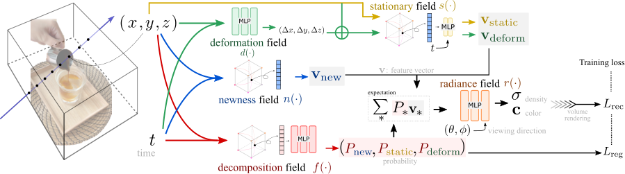
As illustrated in Fig. 2, we assume three kinds of areas in a dynamic scene and model these areas with separate fields:
- •
Static areas have a constant geometry and location in the dynamic scene, such as the table. Besides, we assume the appearance of the static areas will not change frequently over time, i.e., is temporally low-frequency. This is based on the observation that the appearance change is mainly caused by lighting conditions and the albedo is time-invariant. Hence a stationary field is used for representing static points.
- •
Deforming areas model objects with deforming surfaces, such as the hand and the cup in Fig. 2. Deforming areas may comprise rigid or non-rigid motion, but they are always presented in the sequence of interest. Deforming points are represented by a deformation field . Then the deformed point is sent as the query point into a predefined canonical space (e.g., the static field ).
- •
New areas model new content emerging at some point in the sequence, such as the new fluid after pouring espresso into water. A newness feature field with inputs is adopted for representing new areas.
To decompose the scene, we design a decomposition field , where denotes the probability of being static, deforming and new. Next, we consider the output of the fields mentioned above () to be feature vectors rather than properties like the density of the point and denote the output feature vector as , respectively. Finally, given a query point , we first collect the outputs from the above fields and then compute the expected feature vector of this point by , where . Then is sent to a lightweight view-conditioned network for density and color prediction.
In Fig. 3, we demonstrate our approach using a simple 2D toy example. The task studied in the figure is a temporal interpolation from the given 2D images. The fields mentioned above take locations as the input. The string ‘2022’ undergoes rigid motion while the string ‘VR’ gradually appears. The different interpolation performance demonstrates the necessity of modeling dynamic scenes with both deforming and new fields. Note that we do not manually annotate the probability when performing decomposition. Instead, the decomposition field is only supervised by the reconstruction loss and generic parsimony priors which penalize objects being modeled as new. More details about training will be introduced in Section 4.4.
Hybrid representations, which enable fast training and real-time rendering, are adopted for implementing the above neural fields. However, most of existing static scene targeted hybrid representations implement the mapping . Adapting to inputs with an extra dimension time (i.e., dynamic scenes) is not straightforward, since modeling 4D inputs with the explicit representation may significantly increase the model size. A streamable hybrid representation for efficient spatiotemporal mapping is introduced in the next section.
4.2 Streamable Hybrid Representation
We observe that the explicit representation commonly consists of array entries with a predefined feature dimension. For example, each entry in the hash table in InstantNGP instantngp and each basis vector/matrix in TensoRF tensorf both have a fixed feature dimension. Thus, we propose to stream the feature channels so that can be a mapping from a spatiotemporal point to the fixed-length feature vector .
We propose to select feature channels with a sliding window along with the time dimension , as demonstrated in Fig. 4. Assume that for each frame the feature vector is of dimension and channels are newly needed for a new frame, then for a frame sequence the array entry in is of dimension . For a single frame , the channels in will be used for computing , such as trilinear interpolation in InstantNGP or tensor multiplication in TensoRF.
To ensure smoothly translates along with , a rearrangement of feature channels is conducted to match the shared channels. For example, let and , then channels of are used for . Next, we use channels for and channels for . The principle behind the rearrangement is that shared feature channels are always aligned to be with the same index in the vector. Otherwise, a smooth translation between frames is not guaranteed.
The streaming channels readily enable us to temporally interpolate a frame between two observed frames and by linearly interpolating the feature vectors: . Note that our proposed method can be applied to any hybrid representation that contains entries of feature vectors. The implementation of employed will be referred to as backbone in the following text. The sliding window scheme brings two benefits: First, overlapping feature channels are forced to be shared in adjacent frames, thus reducing the model size; Second, after rendering one frame, only new feature channels need to be loaded when moving to the subsequent frames, thus being streaming friendly.
4.3 Overall Framework.
Now we introduce the details of implementing the decomposed spatiotemporal representation (Section 4.1) with the streamable hybrid representation (Section 4.2). An illustration is presented in Fig. 5. The decomposition field consists of explicitly cached features (denoted by ) and a small MLP decoder . The deformation field is an MLP since the deformation is sparse and of low-frequency, where a small MLP is enough. The stationary field consists of explicitly cached features (denoted by ) and a tiny MLP decoder. Time and feature obtained from will be the input to the tiny MLP. The reason for using a tiny MLP is for modeling time-dependent appearance changes caused by time-varying illumination, which is assumed to be of low-frequency. The newness field is explicitly saved features . Note that in the above explicit representations, both and take in a 4D input , hence streaming channels are used here. The final expected feature vector is then decoded by a radiance field . Viewing direction is also sent to as in NeRF.
4.4 Optimization
Training.
Our training process follows the practice of NeRF. A batch of camera rays is first randomly sampled from the observed data and then points on those rays, denoted by , are sampled for training.
In practical reconstruction and rendering tasks, a precise supervisory signal to the decomposition field is inaccessible. Instead, we supervise the output probabilities with a global parsimony regularization. Therefore, besides the reconstruction loss defined in Eq. 2, a regularization loss is introduced in our method. We use the average probability of all points in the batch for this loss, denoted as , where is the number of points. In our implementation, assuming the existence of static background, we propose to minimize the probability of not being a static point, thus the regularization loss is chosen as
| (3) |
where is a tunable parameter for weighting the ratio of being deforming and new. Minimizing the probability of being new points in Eq. 3 relies on the assumption that most of the points in the dynamic scene are either static or deforming. Overall, our training loss is
| (4) |
where is a balancing hyper-parameter.
Rendering.
When rendering an image with a given camera pose, we first forward the sampled points using the decomposition field. After knowing the probabilities, we can skip the forwarding process of some fields for efficiency. With a predefined threshold , if then we directly set and skip the field. We set as 0.001 in our implementation.
5 Experiments
We first quantitatively and qualitatively compare our method with prior works, then extensive ablation studies are presented to validate our proposed components. We urge the reader to watch our video to better appreciate the efficiency and rendering quality of our system.
|
| ||||
|---|---|---|---|---|---|
|
| ||||
|
|


 |
 |
| DyNeRF Li_2022_CVPR | Ours-TensoRF-VM |
Datasets.
Our method requires only RGB observations of the dynamic scene for reconstruction. Unlike most existing methods, our framework does not require special capturing settings or prior knowledge, and detailed comparisons of the framework’s requirements against competitive methods are attached in the supplementary. Two multi-camera datasets and one single-camera dataset are used:
- •
Immersive Video broxton2020immersive includes synchronized videos from 46 4K fisheye cameras. For the raw video data provided by the authors, each camera has different imaging parameters like exposure and white balance. We select 7 dynamic scenes with relatively similar imaging parameters. We downsample the images to in our experiments. The camera with ID 0 (the central camera) is used for validation and the other cameras are used for training.
- •
Plenoptic Video Li_2022_CVPR is captured with 21 cameras at a resolution of . Different from Immersive Video which mostly focuses on outdoor scenes, Plenoptic Video consists of indoor activities in various lighting conditions. We downsample images to in our experiments. We follow the training and validation camera split provided by Li_2022_CVPR. Six scenes are publically available.
- •
HyperNeRF nerfies; park2021hypernerf provides only one view for each timestamp in a dynamic scene. The dataset is challenging due to the single-camera setting. We adopt the same training and validation settings as in park2021hypernerf: images of are used for quantitative evaluation and images of are used for qualitative comparisons. There are two capturing settings in HyperNeRF: “vrig” captures the scene with stereo cameras and training with one camera and validating with the other; “interp” is a monocular video from a moving camera capturing dynamic scenes.
Implementation details.
Our framework, as demonstrated by Fig. 5, is implemented with PyTorch paszke2019pytorch. As highlighted in Section 4.3, our framework is general and any hybrid representation adopting explicit features can be used. We implement our framework with two backbones: InstantNGP instantngp and TensoRF tensorf. In both of the implementations, the deformation network is a 4-layer MLP with a width of 256. The stationary field uses a 2-layer MLP with a width of 64. The radiance field is a 4-layer MLP with a width of 64 and has the same structure as the decoder in the backbone. For InstantNGP based model, the number of levels is 8 and the number of feature dimensions per entry is 4. TensoRF based model follows the same setting as in their experiments on the real forward-facing datasets (i.e., LLFF llff). For both of the two backbones, we set the number of channels for streaming to be 1, and loss hyper-parameters , . We follow the default optimization schedule and settings as in the static-scene targeted backbone methods. For the two multi-camera datasets, we observe that their frame rates are high and simply modeling every dynamic area as new areas already lead to good temporal interpolation performance, so the deformation is not used by default for efficiency. An ablation is presented for studying the impact of video FPS when modeling with and without deformation decomposition. Due to the limitation of model sizes, we split a long video into 90-frame clips and trained on these clips separately. PSNR and SSIM ssim are reported for evaluating the rendering performance.
| Method | PSNR | Training Time | Rendering Time |
|---|---|---|---|
| (GPU Hours) | (s/img) | ||
| Neural Volumes lombardi2019neural | 22.797 | - | - |
| LLFF llff | 23.238 | - | - |
| NeRF-T Li_2022_CVPR | 28.448 | - | 90 |
| DyNeRF Li_2022_CVPR | 29.580 | 1344 | 90 |
| Ours-InstantNGP | 30.293 | 5.5 | 10.8 |
| Ours-TensoRF-VM | 30.692 | 6 | 22.1 |
| Method | Rendering Time | Broom | 3D Printer | Chicken | Peel Banana | Mean | |||||
|---|---|---|---|---|---|---|---|---|---|---|---|
| (s/img) | PSNR | SSIM | PSNR | SSIM | PSNR | SSIM | PSNR | SSIM | PSNR | SSIM | |
| NeRF mildenhall2020nerf | 75 | 19.9 | 0.653 | 20.7 | 0.780 | 19.9 | 0.777 | 20.0 | 0.769 | 20.1 | 0.745 |
| NV lombardi2019neural | 0.03 | 17.7 | 0.623 | 16.2 | 0.665 | 17.6 | 0.615 | 15.9 | 0.380 | 16.9 | 0.571 |
| NSFF nsff∗ | 90 | 26.1 | 0.871 | 27.7 | 0.947 | 26.9 | 0.944 | 24.6 | 0.902 | 26.3 | 0.916 |
| Nerfies nerfies | 90 | 19.2 | 0.567 | 20.6 | 0.830 | 26.7 | 0.943 | 22.4 | 0.872 | 22.2 | 0.803 |
| HyperNeRF park2021hypernerf | 90 | 19.3 | 0.591 | 20.0 | 0.821 | 26.9 | 0.948 | 23.3 | 0.896 | 22.4 | 0.814 |
| Ours-InstantNGP | 4.8 | 21.7 | 0.635 | 22.9 | 0.810 | 26.3 | 0.905 | 24.0 | 0.863 | 23.7 | 0.803 |
 |
 |
 |
 |
 |
 |
 |
 |
 |
 |
 |
 |
 |
 |
| GT | Ours-InstantNGP | HyperNeRF park2021hypernerf | Nerfies nerfies | NSFF nsff | NV lombardi2019neural | NeRF mildenhall2020nerf |
5.1 Comparison with State-of-The-Art Methods
DyNeRF Li_2022_CVPR and HyperNeRF park2021hypernerf are considered for multi- and single-camera settings. Besides the two methods, we also quote the results of other baseline methods reported in their paper.
5.1.1 On multi-camera dataset
In Table 1, we report out results with both InstantNGP and TensoRF backbones. Training time and rendering time of DyNeRF are quoted from their paper. Our method reaches a higher PSNR while significantly reducing the training and rendering time. We further compare the rendered images in Fig. 6. Images of comparison methods are again quoted from the result images in DyNeRF’s paper. Our method with InstantNGP renders images with 12% of the time required by DyNeRF while being comparable. Besides, our method with TensoRF-VM achieves better performance on fast-moving objects. As demonstrated in Fig. 7, we compare our rendered results with extracted frames from DyNeRF’s result video. Since the code and rendering parameters of DyNeRF are not publically available, we manually select similar camera poses and timestamp for comparison. We can observe that the knife in DyNeRF’s results is blurry while our method yields clearer results.
5.1.2 On single-camera dataset
A challenging and practical appealing setting is reconstructing and rendering without per-frame multi-view observations, i.e., capturing with a single camera. Our method with TensoRF backbone is not reported on this dataset since we find that the GPU memory required for training is too large with the default model setting. We compare our method with SoTA single-camera reconstruction methods in Table 2. Note that NSFF requires data-driven depth and optical flow priors. We can observe that our method outperforms HyperNeRF in terms of PSNR but is slightly worse than HyperNeRF on SSIM. We presume the reason is that our method generates more accurate but less sharp images compared to HyperNeRF. Visual comparisons can be found at Fig. 8. We can observe that HyperNeRF sometimes has misalignment between the rendered and real images regarding moving objects, such as the wire in the second row. We attribute the misalignment problem to not correctly modeling the deformation. The incorrect modeling is partially caused by treating all pointing as deforming in their representation. Lacking decomposing static and dynamic areas also leads to a flickering background (demonstrated in our video). In our method, by decomposing static and dynamic areas, the deformation field is regularized to only model dynamic areas.
5.2 Ablation Studies
5.2.1 Impact of Decomposition
We first study the necessity of the proposed three categories for decomposition. Visual comparisons of different decomposition variants are demonstrated in Fig. 10 and quantitative results are reported in Table 3. First, we study the impact of decomposing deforming and new areas on a single-camera dataset. We can observe from Fig. 10(a) that removing new area decomposition leads to failure of modeling the newly poured out espresso and removing deforming area decomposition leads to a blurred hand and cup. Second, we study the impact of our decomposition on the multi-camera dataset. Fig. 10(b) demonstrates that the static area becomes sharper after decomposing static areas. Besides, without static area decomposition, we observe that the background is flickering as we render images with novel time and view.
Finally, we study the impact of deforming area decomposition on the multi-camera dataset. This ablation study is motivated by the observation that rendering with and without deformation modeling leads to little difference (PSNR difference less than 0.1). We presume that this is because the motion of objects between frames is small from cameras with a high FPS recording rate. Therefore modeling all dynamic areas with a newness field can still produce a smooth interpolation. We manually downsample the frame sampling rate for training in Fig. 10(c) to enlarge the motion between frames. We can observe that without deformation modeling the moving helmet becomes first disappeared and then reappeared when interpolating between two training timestamps. As a comparison, the content of the helmet is well preserved if the deformation is modeled.
 |
| (a) Results after removing deforming and new area decomposition on the single-camera dataset (HyperNeRF). |
 |
| (b) Ablation of static area decomposition on the multi-camera dataset (Immersive Video). Second row: novel time and view rendering. |
 |
| (c) Ablation of deforming area decomposition on the multi-camera dataset (Immersive Video). Every 8 frames are used for training. |


| Method | PSNR | SSIM | LPIPS | LPIPS |
|---|---|---|---|---|
| on HyperNeRF-interp | ||||
| w/o deforming | 28.2 | 0.820 | 0.358 | 0.220 |
| w/o new | 28.2 | 0.837 | 0.323 | 0.188 |
| full | 29.2 | 0.858 | 0.294 | 0.163 |
| on Immersive Video (“Horse”) | ||||
| w/o static | 27.0 | 0.860 | 0.423 | 0.255 |
| w/ static | 27.4 | 0.871 | 0.425 | 0.295 |
| on Immersive Video (“Welder” with every 8 frames) | ||||
| w/o deforming | 26.1 | 0.826 | 0.366 | 0.195 |
| w/ deforming | 25.2 | 0.800 | 0.327 | 0.168 |
5.2.2 Scene Decomposition Regularizing
In our method, we use to balance the ratio of being deforming and new in Eq. 3. A larger encourages the scene to contain fewer deforming areas. As introduced in the previous section, single-camera datasets are more sensitive to the deformation field, thus we study the impact of in Fig. 11 on a scene from HyperNeRF. We can observe that over-suppressing deforming areas () lead to blurry moving objects and under-suppressing deforming areas () leads to a noisy scene. The reason behind the blur from large is the same as the second row in Fig. 3 and Fig. 10(c): falsely modeling a moving object as first-disappear-then-reappear. A good practice is that we can start with a relatively large to penalize deforming areas and then gradually allow areas to deform by decreasing .
5.2.3 Streaming Bitrates
An important metric for a streaming service is the bitrate. To render a new frame, the user is usually sensitive to the new data needed to download. We can easily tune the bitrate requirements in our method by setting the value of . In Table 4, we report the bitrate for streaming a new frame with different values. The testing data is a sequence from Immersive Video with 90 frames. Note that denotes new channels needed for rendering a new frame and rendering the first frame still follows the channels required for static scenes (96 for TensoRF-CP and 4 for TensoRF-VM). For fair comparisons, bitrate is computed by the total model size over the number of frames.
The TensoRF-CP based model achieves low bitrate and reasonable performance, while the cost of TensoRF-VM is higher but the performance gain is obvious. We further present rendering results in Fig. 12. We can observe clearer details of the background (i.e., car) and the moving objects (i.e., person) with increased bitrate budgets. The above results validate the extensibility of our framework.
| Method | PSNR | SSIM | LPIPS |
| ||
|---|---|---|---|---|---|---|
| Immersive broxton2020immersive | - | - | - | 0.5 | ||
| Ours-TensoRF-CP | ||||||
| k=0.50 | 25.200 | 0.754 | 0.284 | 0.041 | ||
| k=1.00 | 25.798 | 0.846 | 0.264 | 0.058 | ||
| k=4.00 | 25.870 | 0.835 | 0.266 | 0.114 | ||
| k=16.00 | 25.885 | 0.857 | 0.244 | 0.333 | ||
| Ours-TensoRF-VM | ||||||
| k=0.05 | 26.093 | 0.866 | 0.184 | 3.423 | ||
| k=0.25 | 26.032 | 0.865 | 0.188 | 6.357 | ||
| k=0.50 | 26.187 | 0.872 | 0.192 | 9.942 | ||
| k=1.00 | 26.203 | 0.878 | 0.173 | 17.112 | ||
5.2.4 Rendering Speed and Quality
The performance of our framework is highly correlated with the chosen backbones. Thus, in our method, there exists a tradeoff between rendering speed and quality, mainly affected by predefined model size and rendering hyper-parameters. In Fig. 9, we present the rendering FPS and PSNR with different hyper-parameter settings. We consider two parameters: for the hash table size and the stepping value during ray marching. Scenes from the Immersive Video dataset are considered. We can observe that our method inherits the flexibility of the backbone and we can easily tune the parameters to obtain the desired speed and quality.
 |
 |
 |
| Input images | Novel view | |
6 Limitation and Failure Cases
Our method models each frame in the scene with local feature channels, which enables streaming but limits the representation of long-range repeated activities. For example, the activity of pouring espresso in Fig. 2 may repeat several times in a scene. Further modeling the repeating activities can reduce redundancy and improve the reconstruction quality by leveraging all the views of the same object. Moreover, our method assumes input multi-view images are with the same camera imaging configuration (e.g., exposure). A failure example from Immersive Video is demonstrated in Fig. 13. Though view dependency can still be modeled in the framework, the model tends to generate floating points to overfit the training views. Recent progress that considers the photography process martin2021nerf; mildenhall2021rawnerf may help solve the issue.
7 Conclusion
We present a framework for representing dynamic scenes from both multi- and single-camera captured images. The key components of our framework are the decomposition module and the feature streaming module. The decomposition module decomposes the scene into static, deforming, and new areas. A sliding window based hybrid representation is then designed for efficiently modeling the decomposed neural fields. Experiments on multi- and single-camera datasets validate our method’s efficiency and effectiveness. Extensive ablation studies further provide insight into the model design, such as the necessity of modeling deformation in large-motion scenes captured by camera arrays.
References
- (1) Benjamin Attal, Jia-Bin Huang, Christian Richardt, Michael Zollhoefer, Johannes Kopf, Matthew O’Toole, and Changil Kim. HyperReel: High-fidelity 6-DoF video with ray-conditioned sampling. arXiv preprint arXiv:2301.02238, 2023.
- (2) Aayush Bansal, Minh Vo, Yaser Sheikh, Deva Ramanan, and Srinivasa Narasimhan. 4d visualization of dynamic events from unconstrained multi-view videos. In Proceedings of the IEEE/CVF Conference on Computer Vision and Pattern Recognition, pages 5366–5375, 2020.
- (3) Mojtaba Bemana, Karol Myszkowski, Hans-Peter Seidel, and Tobias Ritschel. X-fields: Implicit neural view-, light-and time-image interpolation. ACM Transactions on Graphics (TOG), 39(6):1–15, 2020.
- (4) Mark Boss, Raphael Braun, Varun Jampani, Jonathan T Barron, Ce Liu, and Hendrik Lensch. Nerd: Neural reflectance decomposition from image collections. In Proceedings of the IEEE/CVF International Conference on Computer Vision, pages 12684–12694, 2021.
- (5) Mark Boss, Varun Jampani, Raphael Braun, Ce Liu, Jonathan T. Barron, and Hendrik P.A. Lensch. Neural-pil: Neural pre-integrated lighting for reflectance decomposition. In Advances in Neural Information Processing Systems, 2021.
- (6) Michael Broxton, John Flynn, Ryan Overbeck, Daniel Erickson, Peter Hedman, Matthew Duvall, Jason Dourgarian, Jay Busch, Matt Whalen, and Paul Debevec. Immersive light field video with a layered mesh representation. ACM Transactions on Graphics (TOG), 39(4):86–1, 2020.
- (7) Ang Cao and Justin Johnson. Hexplane: A fast representation for dynamic scenes. arXiv:2301.09632, 2023.
- (8) Joel Carranza, Christian Theobalt, Marcus A Magnor, and Hans-Peter Seidel. Free-viewpoint video of human actors. ACM transactions on graphics (TOG), 22(3):569–577, 2003.
- (9) Eric R. Chan, Connor Z. Lin, Matthew A. Chan, Koki Nagano, Boxiao Pan, Shalini De Mello, Orazio Gallo, Leonidas Guibas, Jonathan Tremblay, Sameh Khamis, Tero Karras, and Gordon Wetzstein. In Proceedings of the IEEE/CVF Conference on Computer Vision and Pattern Recognition, pages 16123–16133, 2022.
- (10) Eric R Chan, Marco Monteiro, Petr Kellnhofer, Jiajun Wu, and Gordon Wetzstein. pi-gan: Periodic implicit generative adversarial networks for 3d-aware image synthesis. In Proceedings of the IEEE/CVF Conference on Computer Vision and Pattern Recognition, pages 5799–5809, 2021.
- (11) Anpei Chen, Zexiang Xu, Andreas Geiger, Jingyi Yu, and Hao Su. Tensorf: Tensorial radiance fields. In Proceedings of the European Conference on Computer Vision, 2022.
- (12) Julian Chibane, Gerard Pons-Moll, et al. Neural unsigned distance fields for implicit function learning. Advances in Neural Information Processing Systems, 33, 2020.
- (13) Alvaro Collet, Ming Chuang, Pat Sweeney, Don Gillett, Dennis Evseev, David Calabrese, Hugues Hoppe, Adam Kirk, and Steve Sullivan. High-quality streamable free-viewpoint video. ACM Transactions on Graphics (ToG), 34(4):1–13, 2015.
- (14) Yilun Du, Yinan Zhang, Hong-Xing Yu, Joshua B. Tenenbaum, and Jiajun Wu. Neural radiance flow for 4d view synthesis and video processing. In Proceedings of the IEEE/CVF International Conference on Computer Vision, 2021.
- (15) Jiemin Fang, Lingxi Xie, Xinggang Wang, Xiaopeng Zhang, Wenyu Liu, and Qi Tian. Neusample: Neural sample field for efficient view synthesis. arXiv:2111.15552, 2021.
- (16) Jiemin Fang, Taoran Yi, Xinggang Wang, Lingxi Xie, Xiaopeng Zhang, Wenyu Liu, Matthias Nießner, and Qi Tian. Fast dynamic radiance fields with time-aware neural voxels. arXiv preprint arXiv:2205.15285, 2022.
- (17) Sara Fridovich-Keil, Giacomo Meanti, Frederik Rahbæk Warburg, Benjamin Recht, and Angjoo Kanazawa. K-planes: Explicit radiance fields in space, time, and appearance, 2023.
- (18) Wanshui Gan, Hongbin Xu, Yi Huang, Shifeng Chen, and Naoto Yokoya. V4d: Voxel for 4d novel view synthesis. arXiv preprint arXiv:2205.14332, 2022.
- (19) Hang Gao, Ruilong Li, Shubham Tulsiani, Bryan Russell, and Angjoo Kanazawa. Monocular dynamic view synthesis: A reality check. In Neural Information Processing Systems (Neurips), 2022.
- (20) Stephan J. Garbin, Marek Kowalski, Matthew Johnson, Jamie Shotton, and Julien Valentin. Fastnerf: High-fidelity neural rendering at 200fps. In Proceedings of the IEEE/CVF International Conference on Computer Vision, pages 14346–14355, October 2021.
- (21) Steven J. Gortler, Radek Grzeszczuk, Richard Szeliski, and Michael F. Cohen. The lumigraph. In John Fujii, editor, SIGGRAPH, pages 43–54. ACM, 1996.
- (22) Jiatao Gu, Lingjie Liu, Peng Wang, and Christian Theobalt. Stylenerf: A style-based 3d aware generator for high-resolution image synthesis. In International Conference on Learning Representations, 2021.
- (23) Peter Hedman, Pratul P. Srinivasan, Ben Mildenhall, Jonathan T. Barron, and Paul Debevec. Baking neural radiance fields for real-time view synthesis. In Proceedings of the IEEE/CVF International Conference on Computer Vision, pages 5875–5884, October 2021.
- (24) Yang Hong, Bo Peng, Haiyao Xiao, Ligang Liu, and Juyong Zhang. Headnerf: A real-time nerf-based parametric head model. In Proceedings of the IEEE/CVF Conference on Computer Vision and Pattern Recognition, pages 20374–20384, 2022.
- (25) Ajay Jain, Ben Mildenhall, Jonathan T Barron, Pieter Abbeel, and Ben Poole. Zero-shot text-guided object generation with dream fields. In Proceedings of the IEEE/CVF Conference on Computer Vision and Pattern Recognition, pages 867–876, 2022.
- (26) Ramesh Jain and Koji Wakimoto. Multiple perspective interactive video. In Proceedings of the international conference on multimedia computing and systems, pages 202–211. IEEE, 1995.
- (27) Hankyu Jang and Daeyoung Kim. D-tensorf: Tensorial radiance fields for dynamic scenes. ArXiv, abs/2212.02375, 2022.
- (28) Takeo Kanade, Peter Rander, and PJ Narayanan. Virtualized reality: Constructing virtual worlds from real scenes. IEEE MultiMedia, 4(1):34–47, 1997.
- (29) Sosuke Kobayashi, Eiichi Matsumoto, and Vincent Sitzmann. Decomposing nerf for editing via feature field distillation. In arXiv, 2022.
- (30) Johannes Kopf, Xuejian Rong, and Jia-Bin Huang. Robust consistent video depth estimation. In Proceedings of the IEEE/CVF Conference on Computer Vision and Pattern Recognition, pages 1611–1621, 2021.
- (31) Adam R Kosiorek, Heiko Strathmann, Daniel Zoran, Pol Moreno, Rosalia Schneider, Sona Mokrá, and Danilo Jimenez Rezende. Nerf-vae: A geometry aware 3d scene generative model. In International Conference on Machine Learning, pages 5742–5752. PMLR, 2021.
- (32) Andreas Kurz, Thomas Neff, Zhaoyang Lv, Michael Zollhofer, and Markus Steinberger. Adanerf: Adaptive sampling for real-time rendering of neural radiance fields. In European Conference on Computer Vision, 2022.
- (33) Aviad Levis, Pratul P Srinivasan, Andrew A Chael, Ren Ng, and Katherine L Bouman. Gravitationally lensed black hole emission tomography. In Proceedings of the IEEE/CVF Conference on Computer Vision and Pattern Recognition, pages 19841–19850, 2022.
- (34) Marc Levoy and Pat Hanrahan. Light field rendering. In John Fujii, editor, SIGGRAPH, pages 31–42. ACM, 1996.
- (35) Lingzhi Li, Zhen Shen, Zhongshu Wang, Li Shen, and Ping Tan. Streaming radiance fields for 3d video synthesis. In Neural Information Processing Systems (Neurips), 2022.
- (36) Tianye Li, Mira Slavcheva, Michael Zollhöfer, Simon Green, Christoph Lassner, Changil Kim, Tanner Schmidt, Steven Lovegrove, Michael Goesele, Richard Newcombe, and Zhaoyang Lv. Neural 3d video synthesis from multi-view video. In Proceedings of the IEEE/CVF Conference on Computer Vision and Pattern Recognition (CVPR), pages 5521–5531, June 2022.
- (37) Zhengqi Li, Simon Niklaus, Noah Snavely, and Oliver Wang. Neural scene flow fields for space-time view synthesis of dynamic scenes. In Proceedings of the IEEE/CVF Conference on Computer Vision and Pattern Recognition, 2021.
- (38) Haotong Lin, Sida Peng, Zhen Xu, Yunzhi Yan, Qing Shuai, Hujun Bao, and Xiaowei Zhou. Efficient neural radiance fields with learned depth-guided sampling. In SIGGRAPH Asia Conference Proceedings, 2022.
- (39) D. B.* Lindell, J. N. P.* Martel, and G. Wetzstein. Autoint: Automatic integration for fast neural volume rendering. In Proceedings of the IEEE/CVF International Conference on Computer Vision, 2021.
- (40) Jia-Wei Liu, Yan-Pei Cao, Weijia Mao, Wenqiao Zhang, David Junhao Zhang, Jussi Keppo, Ying Shan, Xiaohu Qie, and Mike Zheng Shou. Devrf: Fast deformable voxel radiance fields for dynamic scenes. arXiv preprint arXiv:2205.15723, 2022.
- (41) Lingjie Liu, Jiatao Gu, Kyaw Zaw Lin, Tat-Seng Chua, and Christian Theobalt. Neural sparse voxel fields. In Advances in Neural Information Processing Systems, 2020.
- (42) Lingjie Liu, Marc Habermann, Viktor Rudnev, Kripasindhu Sarkar, Jiatao Gu, and Christian Theobalt. Neural actor: Neural free-view synthesis of human actors with pose control. ACM Trans. Graph.(ACM SIGGRAPH Asia), 2021.
- (43) Renhao Liu, Yu Sun, Jiabei Zhu, Lei Tian, and Ulugbek S Kamilov. Recovery of continuous 3d refractive index maps from discrete intensity-only measurements using neural fields. Nature Machine Intelligence, 4(9):781–791, 2022.
- (44) Stephen Lombardi, Tomas Simon, Jason Saragih, Gabriel Schwartz, Andreas Lehrmann, and Yaser Sheikh. Neural volumes: learning dynamic renderable volumes from images. ACM Transactions on Graphics, 38(4):1–14, 2019.
- (45) Stephen Lombardi, Tomas Simon, Gabriel Schwartz, Michael Zollhöfer, Yaser Sheikh, and Jason M. Saragih. Mixture of volumetric primitives for efficient neural rendering. ACM Trans. Graph., 40(4):59:1–59:13, 2021.
- (46) Xuan Luo, Jia-Bin Huang, Richard Szeliski, Kevin Matzen, and Johannes Kopf. Consistent video depth estimation. ACM Transactions on Graphics (ToG), 39(4):71–1, 2020.
- (47) Ricardo Martin-Brualla, Noha Radwan, Mehdi SM Sajjadi, Jonathan T Barron, Alexey Dosovitskiy, and Daniel Duckworth. Nerf in the wild: Neural radiance fields for unconstrained photo collections. In Proceedings of the IEEE/CVF Conference on Computer Vision and Pattern Recognition, pages 7210–7219, 2021.
- (48) Lars Mescheder, Michael Oechsle, Michael Niemeyer, Sebastian Nowozin, and Andreas Geiger. Occupancy networks: Learning 3d reconstruction in function space. In Proceedings of the IEEE/CVF Conference on Computer Vision and Pattern Recognition, pages 4460–4470, 2019.
- (49) Ben Mildenhall, Peter Hedman, Ricardo Martin-Brualla, Pratul P Srinivasan, and Jonathan T Barron. Nerf in the dark: High dynamic range view synthesis from noisy raw images. In Proceedings of the IEEE/CVF Conference on Computer Vision and Pattern Recognition, pages 16190–16199, 2022.
- (50) Ben Mildenhall, Pratul P. Srinivasan, Rodrigo Ortiz-Cayon, Nima Khademi Kalantari, Ravi Ramamoorthi, Ren Ng, and Abhishek Kar. Local light field fusion: Practical view synthesis with prescriptive sampling guidelines. ACM Transactions on Graphics (Proceedings of SIGGRAPH), 38(4), 2019.
- (51) Ben Mildenhall, Pratul P Srinivasan, Matthew Tancik, Jonathan T Barron, Ravi Ramamoorthi, and Ren Ng. Nerf: Representing scenes as neural radiance fields for view synthesis. In European Conference on Computer Vision, pages 405–421. Springer, 2020.
- (52) Thomas Müller, Alex Evans, Christoph Schied, and Alexander Keller. Instant neural graphics primitives with a multiresolution hash encoding. ACM Trans. Graph., 41(4):102:1–102:15, July 2022.
- (53) Thomas Neff, Pascal Stadlbauer, Mathias Parger, Andreas Kurz, Joerg H. Mueller, Chakravarty R. Alla Chaitanya, Anton S. Kaplanyan, and Markus Steinberger. DONeRF: Towards Real-Time Rendering of Compact Neural Radiance Fields using Depth Oracle Networks. Computer Graphics Forum, 40(4), 2021.
- (54) Michael Niemeyer, Lars Mescheder, Michael Oechsle, and Andreas Geiger. Occupancy flow: 4d reconstruction by learning particle dynamics. In Proceedings of the IEEE/CVF international conference on computer vision, pages 5379–5389, 2019.
- (55) Atsuhiro Noguchi, Xiao Sun, Stephen Lin, and Tatsuya Harada. Neural articulated radiance field. In Proceedings of the IEEE/CVF International Conference on Computer Vision, pages 5762–5772, October 2021.
- (56) Julian Ost, Fahim Mannan, Nils Thuerey, Julian Knodt, and Felix Heide. Neural scene graphs for dynamic scenes. In Proceedings of the IEEE/CVF Conference on Computer Vision and Pattern Recognition, pages 2856–2865, 2021.
- (57) Jeong Joon Park, Peter Florence, Julian Straub, Richard Newcombe, and Steven Lovegrove. Deepsdf: Learning continuous signed distance functions for shape representation. In Proceedings of the IEEE/CVF Conference on Computer Vision and Pattern Recognition, pages 165–174, 2019.
- (58) Keunhong Park, Utkarsh Sinha, Jonathan T. Barron, Sofien Bouaziz, Dan B Goldman, Steven M. Seitz, and Ricardo Martin-Brualla. Nerfies: Deformable neural radiance fields. In Proceedings of the IEEE/CVF International Conference on Computer Vision, pages 5865–5874, October 2021.
- (59) Keunhong Park, Utkarsh Sinha, Peter Hedman, Jonathan T. Barron, Sofien Bouaziz, Dan B Goldman, Ricardo Martin-Brualla, and Steven M. Seitz. Hypernerf: A higher-dimensional representation for topologically varying neural radiance fields. ACM Trans. Graph., 40(6), dec 2021.
- (60) Adam Paszke, Sam Gross, Francisco Massa, Adam Lerer, James Bradbury, Gregory Chanan, Trevor Killeen, Zeming Lin, Natalia Gimelshein, Luca Antiga, et al. Pytorch: An imperative style, high-performance deep learning library. Advances in neural information processing systems, 32:8026–8037, 2019.
- (61) Sida Peng, Junting Dong, Qianqian Wang, Shangzhan Zhang, Qing Shuai, Xiaowei Zhou, and Hujun Bao. Animatable neural radiance fields for modeling dynamic human bodies. In Proceedings of the IEEE/CVF International Conference on Computer Vision, pages 14314–14323, October 2021.
- (62) Sida Peng, Yuanqing Zhang, Yinghao Xu, Qianqian Wang, Qing Shuai, Hujun Bao, and Xiaowei Zhou. Neural body: Implicit neural representations with structured latent codes for novel view synthesis of dynamic humans. In Proceedings of the IEEE/CVF Conference on Computer Vision and Pattern Recognition, pages 9054–9063, 2021.
- (63) Martin Piala and Ronald Clark. Terminerf: Ray termination prediction for efficient neural rendering. International Conference on 3D Vision, pages 1106–1114, 2021.
- (64) Albert Pumarola, Enric Corona, Gerard Pons-Moll, and Francesc Moreno-Noguer. D-nerf: Neural radiance fields for dynamic scenes. In Proceedings of the IEEE/CVF Conference on Computer Vision and Pattern Recognition, pages 10318–10327, 2021.
- (65) Daniel Rebain, Wei Jiang, Soroosh Yazdani, Ke Li, Kwang Moo Yi, and Andrea Tagliasacchi. Derf: Decomposed radiance fields. In Proceedings of the IEEE/CVF Conference on Computer Vision and Pattern Recognition, pages 14153–14161, 2021.
- (66) Christian Reiser, Songyou Peng, Yiyi Liao, and Andreas Geiger. Kilonerf: Speeding up neural radiance fields with thousands of tiny mlps. In Proceedings of the IEEE/CVF International Conference on Computer Vision, pages 14335–14345, October 2021.
- (67) Sara Fridovich-Keil and Alex Yu, Matthew Tancik, Qinhong Chen, Benjamin Recht, and Angjoo Kanazawa. Plenoxels: Radiance fields without neural networks. In Proceedings of the IEEE/CVF Conference on Computer Vision and Pattern Recognition, 2022.
- (68) Hartmut Schirmacher, Li Ming, and Hans-Peter Seidel. On-the-fly processing of generalized lumigraphs. In Computer Graphics Forum, volume 20, pages 165–174. Wiley Online Library, 2001.
- (69) Katja Schwarz, Yiyi Liao, Michael Niemeyer, and Andreas Geiger. Graf: Generative radiance fields for 3d-aware image synthesis. Advances in Neural Information Processing Systems, 33, 2020.
- (70) Prafull Sharma, Ayush Tewari, Yilun Du, Sergey Zakharov, Rares Ambrus, Adrien Gaidon, William T Freeman, Frédo Durand, Joshua B Tenenbaum, and Vincent Sitzmann. Seeing 3d objects in a single image via self-supervised static-dynamic disentanglement. arXiv preprint arXiv:2207.11232, 2022.
- (71) Pratul P Srinivasan, Boyang Deng, Xiuming Zhang, Matthew Tancik, Ben Mildenhall, and Jonathan T Barron. Nerv: Neural reflectance and visibility fields for relighting and view synthesis. In Proceedings of the IEEE/CVF Conference on Computer Vision and Pattern Recognition, pages 7495–7504, 2021.
- (72) Shih-Yang Su, Frank Yu, Michael Zollhoefer, and Helge Rhodin. A-nerf: Articulated neural radiance fields for learning human shape, appearance, and pose. In NeurIPS, 2021.
- (73) Cheng Sun, Min Sun, and Hwann-Tzong Chen. Direct voxel grid optimization: Super-fast convergence for radiance fields reconstruction. In Proceedings of the IEEE/CVF Conference on Computer Vision and Pattern Recognition, pages 5459–5469, 2022.
- (74) Towaki Takikawa, Alex Evans, Jonathan Tremblay, Thomas Müller, Morgan McGuire, Alec Jacobson, and Sanja Fidler. Variable bitrate neural fields. In ACM SIGGRAPH Conference Proceedings, pages 1–9, 2022.
- (75) Towaki Takikawa, Joey Litalien, Kangxue Yin, Karsten Kreis, Charles Loop, Derek Nowrouzezahrai, Alec Jacobson, Morgan McGuire, and Sanja Fidler. Neural geometric level of detail: Real-time rendering with implicit 3d shapes. In Proceedings of the IEEE/CVF Conference on Computer Vision and Pattern Recognition, pages 11358–11367, 2021.
- (76) Matthew Tancik, Vincent Casser, Xinchen Yan, Sabeek Pradhan, Ben Mildenhall, Pratul P Srinivasan, Jonathan T Barron, and Henrik Kretzschmar. Block-nerf: Scalable large scene neural view synthesis. In Proceedings of the IEEE/CVF Conference on Computer Vision and Pattern Recognition, pages 8248–8258, 2022.
- (77) Edgar Tretschk, Ayush Tewari, Vladislav Golyanik, Michael Zollhöfer, Christoph Lassner, and Christian Theobalt. Non-rigid neural radiance fields: Reconstruction and novel view synthesis of a dynamic scene from monocular video. In Proceedings of the IEEE/CVF International Conference on Computer Vision, pages 12959–12970, October 2021.
- (78) Alex Trevithick and Bo Yang. Grf: Learning a general radiance field for 3d representation and rendering. In Proceedings of the IEEE/CVF International Conference on Computer Vision, pages 15182–15192, October 2021.
- (79) Vadim Tschernezki, Iro Laina, Diane Larlus, and Andrea Vedaldi. Neural Feature Fusion Fields: 3D distillation of self-supervised 2D image representations. In Proceedings of the International Conference on 3D Vision (3DV), 2022.
- (80) Vadim Tschernezki, Diane Larlus, and Andrea Vedaldi. Neuraldiff: Segmenting 3d objects that move in egocentric videos. In International Conference on 3D Vision (3DV), pages 910–919. IEEE, 2021.
- (81) Chaoyang Wang, Ben Eckart, Simon Lucey, and Orazio Gallo. Neural trajectory fields for dynamic novel view synthesis. arXiv preprint arXiv:2105.05994, 2021.
- (82) Liao Wang, Jiakai Zhang, Xinhang Liu, Fuqiang Zhao, Yanshun Zhang, Yingliang Zhang, Minye Wu, Jingyi Yu, and Lan Xu. Fourier plenoctrees for dynamic radiance field rendering in real-time. In Proceedings of the IEEE/CVF Conference on Computer Vision and Pattern Recognition, pages 13524–13534, 2022.
- (83) Zhou Wang, Alan C Bovik, Hamid R Sheikh, and Eero P Simoncelli. Image quality assessment: from error visibility to structural similarity. IEEE transactions on image processing, 13(4):600–612, 2004.
- (84) Suttisak Wizadwongsa, Pakkapon Phongthawee, Jiraphon Yenphraphai, and Supasorn Suwajanakorn. Nex: Real-time view synthesis with neural basis expansion. In Proceedings of the IEEE/CVF Conference on Computer Vision and Pattern Recognition, pages 8534–8543, 2021.
- (85) Liwen Wu, Jae Yong Lee, Anand Bhattad, Yu-Xiong Wang, and David Forsyth. Diver: Real-time and accurate neural radiance fields with deterministic integration for volume rendering. In Proceedings of the IEEE/CVF Conference on Computer Vision and Pattern Recognition, pages 16200–16209, 2022.
- (86) Tianhao Wu, Fangcheng Zhong, Andrea Tagliasacchi, Forrester Cole, and Cengiz Oztireli. D2nerf: Self-supervised decoupling of dynamic and static objects from a monocular video. arXiv preprint arXiv:2205.15838, 2022.
- (87) Wenqi Xian, Jia-Bin Huang, Johannes Kopf, and Changil Kim. Space-time neural irradiance fields for free-viewpoint video. In Proceedings of the IEEE/CVF Conference on Computer Vision and Pattern Recognition, pages 9421–9431, 2021.
- (88) Yiheng Xie, Towaki Takikawa, Shunsuke Saito, Or Litany, Shiqin Yan, Numair Khan, Federico Tombari, James Tompkin, Vincent Sitzmann, and Srinath Sridhar. Neural fields in visual computing and beyond. In Computer Graphics Forum, volume 41, pages 641–676. Wiley Online Library, 2022.
- (89) Bangbang Yang, Yinda Zhang, Yinghao Xu, Yijin Li, Han Zhou, Hujun Bao, Guofeng Zhang, and Zhaopeng Cui. Learning object-compositional neural radiance field for editable scene rendering. In Proceedings of the IEEE/CVF International Conference on Computer Vision, pages 13779–13788, 2021.
- (90) Jason C Yang, Matthew Everett, Chris Buehler, and Leonard McMillan. A real-time distributed light field camera. Rendering Techniques, 2002:77–86, 2002.
- (91) Alex Yu, Ruilong Li, Matthew Tancik, Hao Li, Ren Ng, and Angjoo Kanazawa. Plenoctrees for real-time rendering of neural radiance fields. In Proceedings of the IEEE/CVF International Conference on Computer Vision, pages 5752–5761, October 2021.
- (92) Wentao Yuan, Zhaoyang Lv, Tanner Schmidt, and Steven Lovegrove. Star: Self-supervised tracking and reconstruction of rigid objects in motion with neural rendering. In Proceedings of the IEEE/CVF Conference on Computer Vision and Pattern Recognition, pages 13144–13152, 2021.
- (93) Jiakai Zhang, Xinhang Liu, Xinyi Ye, Fuqiang Zhao, Yanshun Zhang, Minye Wu, Yingliang Zhang, Lan Xu, and Jingyi Yu. Editable free-viewpoint video using a layered neural representation. ACM Trans. Graph., 40(4):149:1–149:18, 2021.
- (94) Xiaoshuai Zhang, Sai Bi, Kalyan Sunkavalli, Hao Su, and Zexiang Xu. Nerfusion: Fusing radiance fields for large-scale scene reconstruction. In Proceedings of the IEEE/CVF Conference on Computer Vision and Pattern Recognition, pages 5449–5458, 2022.
- (95) C Lawrence Zitnick, Sing Bing Kang, Matthew Uyttendaele, Simon Winder, and Richard Szeliski. High-quality video view interpolation using a layered representation. ACM transactions on graphics (TOG), 23(3):600–608, 2004.
Appendix
Per-scene performance evaluations are presented in Table 5 (for Immersive Video) and Table 6 (for Plenoptic Video).
| Scene | PSNR | SSIM | LPIPSAlex | LPIPSVGG |
|---|---|---|---|---|
| 01_Welder | 25.568 | 0.818 | 0.289 | 0.420 |
| 02_Flames | 26.554 | 0.842 | 0.154 | 0.271 |
| 03_Dog | 18.764 | 0.579 | 0.463 | 0.515 |
| 04_Truck | 27.021 | 0.877 | 0.164 | 0.311 |
| 05_Horse | 27.416 | 0.871 | 0.295 | 0.425 |
| 06_Goats | 23.023 | 0.794 | 0.278 | 0.386 |
| 07_Car | 19.656 | 0.624 | 0.393 | 0.501 |
| 08_Pond | 18.132 | 0.728 | 0.352 | 0.487 |
| 09_Alexa_Meade_Exhibit | 24.549 | 0.869 | 0.151 | 0.278 |
| 10_Alexa_Meade_Face_Paint_1 | 27.772 | 0.916 | 0.147 | 0.314 |
| 11_Alexa_Meade_Face_Paint_2 | 27.352 | 0.902 | 0.152 | 0.326 |
| 12_Cave | 21.825 | 0.715 | 0.314 | 0.381 |
| 13_Birds | 13.776 | 0.826 | 0.318 | 0.451 |
| 14_Puppy | 15.594 | 0.791 | 0.305 | 0.482 |
| Mean (All) | 22.643 | 0.796 | 0.269 | 0.396 |
| Mean (Selected 7) | 26.604 | 0.870 | 0.193 | 0.335 |
(a) Ours-InstantNGP
Scene
PSNR
SSIM
LPIPSAlex
LPIPSVGG
coffee martini
32.053
0.938
0.115
0.279
cook spinach
32.064
0.930
0.116
0.284
cut roasted beef
31.830
0.928
0.119
0.287
flame salmon
26.140
0.849
0.233
0.379
flame steak
27.361
0.867
0.215
0.355
sear steak
32.310
0.940
0.111
0.272
Mean
30.293
0.909
0.152
0.309
(b) Ours-TensoRF-VM
Scene
PSNR
SSIM
LPIPSAlex
LPIPSVGG
coffee martini
31.534
0.951
0.085
0.187
cook spinach
30.557
0.929
0.113
0.226
cut roasted beef
29.353
0.908
0.144
0.221
flame salmon
31.646
0.940
0.098
0.203
flame steak
31.932
0.950
0.088
0.190
sear steak
29.129
0.908
0.138
0.227
Mean
30.692
0.931
0.111
0.209