跳到论文正文
W Papers独立论文阅读器 arXiv:2210.15685 论文正文 计算阅读时间 · 0%
引用这篇论文根据当前论文元数据生成,正式投稿前建议核对。


License: arXiv.org perpetual non-exclusive license
arXiv:2210.15685v2 [gr-qc] 22 Nov 2022

Exotic marginally outer trapped surfaces
in rotating spacetimes of any dimension

Ivan Booth    Kam To Billy Chan    Robie A. Hennigar    Hari Kunduri Affiliation:  Department of Mathematics and Statistics and Department of Physics and Astronomy, McMaster University, Hamilton, Ontario, L8S 4M1, Canada    Sarah Muth
Abstract

The recently developed MOTSodesic method for locating marginally outer trapped surfaces was effectively restricted to non-rotating spacetimes. In this paper we extend the method to include (multi-)axisymmetric time slices of (multi-)axisymmetric spacetimes of any dimension. We then apply this method to study marginally outer trapped surfaces (MOTSs) in the BTZ, Kerr and Myers-Perry black holes. While there are many similarities between the MOTSs observed in these spacetimes and those seen in Schwarzschild and Reissner-Nordström, details of the more complicated geometries also introduce some new, previously unseen, behaviours.

1 Introduction

Trapped surfaces play an indispensable role in the theory of black holes. The existence of a trapped surface is related to the inevitable formation of a spacetime singularity through the Hawking-Penrose singularity theorems [1, 2]. Trapped surfaces lead to a characterization of black holes and their properties that is quasi-local in space and local in time, providing an alternative to the teleological event horizon [3]. As such, these methods are routinely used in numerical relativity, where the ability to locate the black hole horizon at a given moment of time has obvious practical utility [4, 5, 6, 7].

A key object in the quasi-local approach to black hole boundaries is the marginally outer trapped surface (MOTS). In a DD-dimensional spacetime, an outer trapped surface is a closed, space-like (D−2)(D\!\!-\!\!2)-dimensional surface such that light rays emitted in the future outward-pointing null normal directions are converging. A (fully) trapped surface is one for which both inward and outward light rays converge. A MOTS is a limiting case of an outer trapped surface: a closed, space-like (D−2)(D\!\!-\!\!2)-dimensional surface for which the light rays emitted in the future-pointing outward direction are neither converging nor expanding, while no constraint is placed on the light rays emitted in the inward direction. In the simplest black hole spacetimes, for example Schwarzschild, within the event horizon the spheres of constant radius and time are trapped surfaces, while cross-sections of the event horizon are MOTSs.

Many important results from the mathematical theory of black holes can be formulated with reference to either event horizons or MOTSs. For example, MOTSs can be assigned physical quantities, such as mass and angular momentum, and variations in these quantities are constrained, through the Einstein equations, into variational identities analogous to the laws of black hole mechanics [8, 9, 10, 11, 12]. However, theoretical developments in this area have tended to be more difficult than comparable analyses based on the event horizon. Progress toward addressing these questions has partly been illuminated through a better understanding of MOTSs in simpler, exact spacetimes.

An example of this concerns the notion of the “second law”, or area monotonicity theorem, for MOTSs. A number of examples of marginally trapped tubes were studied in [13], where the full hypersurface consisted of both time-like and space-like segments. It was remarked in [13] that the area evolution of the marginally trapped surfaces foliating the tube was monotonic, if one takes the time-like and space-like segments together to form a single entity. It was subsequently proven, with a few additional assumptions,11 1 We now understand that some of these additional assumptions do not apply to certain MOTSs that are present, for example, in the interior of a binary merger [14]. that the area of MOTSs along a marginal tube is indeed monotonic in general [15]. Another example is the “apparent horizon” Penrose inequality, for which a counter-example was found by studying MOTSs in time-dependent spherically symmetric backgrounds [16]. A number of further examples can be found in [17].

A more recent case where there has been positive back-and-forth interaction between exact solution analyses and more general dynamical situations has been in understanding the final fate problem in a black hole collision. That is: what happens to the original black hole horizons (event or apparent) when two black holes merge to become one? In the case of the event horizon, this problem has been well-understood for over half a century. The result is nicely summarized in the well-known “pair of pants” diagram [2]. While some understanding of this problem in the quasi-local paradigm dates back to the same time, much of the progress in resolving this question happened only in the last few years [18, 19, 20, 21, 22, 23] — see [24] for a succinct summary of the current understanding. A number of results that have emerged from this analysis have been important for revealing novel properties of MOTSs, and in clarifying which MOTSs can be appropriately called black hole boundaries.

It was observed in [20, 21] that MOTSs with self-intersections play a role in a binary black hole merger. More specifically, it was found that the inner common MOTS, which forms in a bifurcation with the apparent horizon when the two original black holes become sufficiently close, develops self-intersections after penetrating the MOTSs describing the apparent horizons of the original black holes. This was the first observation of such surfaces, in part because previously existing numerical MOTS finders were built so that they could only find “star-shaped” surfaces. Hence they were blind to surfaces with self-intersections. The key to the work of [20, 21] was the development of a reference-shape based MOTS finder. Subsequently it was shown that self-intersecting MOTSs are, in fact, extremely common [25], when it was found that even within the event horizon of the Schwarzschild space-time there exist an apparently infinite family of self-intersecting MOTSs.

As a short-hand, we will refer to the (now large) class of “new” MOTSs as exotic. This is inspired by their generally complicated geometries, as opposed to the relatively sedate geometries of black hole horizons.

The observation of an infinite number of self-intersecting MOTSs was not the original motivation behind the work [25]. Instead, the aim was to describe the evolution of the apparent horizon during an extreme mass ratio binary black hole merger. This was based on the insights of [26, 27, 28], where the event horizon evolution during a merger was understood exactly in the (strict) extreme mass ratio limit. In this framework, one tracks the paths traced by a sheet of null rays — corresponding to the event horizon of the large black hole — in the spacetime of the small black hole. While a complete analysis of the apparent horizon was not achieved in [25], it was found that a number of structures exist within a single black hole that mimic those seen in a full numerical simulation of colliding black holes. These observations, and the methods used, provided the impetus for the analysis carried out and numerical methods developed in [21, 22, 23].

The work done in [25] found MOTSs using a simple numerical algorithm that made use of the axisymmetry of the spacetime and a shooting method. The problem of finding MOTSs was reduced, via axisymmetry, to the problem of finding curves in the two-dimensional orbit space, or in concrete terms, the (r,θ)(r,\theta)-plane (see Figure 1). As was shown more elegantly in later papers [22, 29], those curves are defined according to the equation

Ta​D¯a​Tb=κ​Nb,T^{a}\bar{D}_{a}T^{b}=\kappa N^{b}\,, (1)

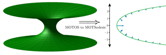
where TaT^{a} is the tangent to the curve, NbN^{b} is its normal, D¯\bar{D} is the two-dimensional covariant derivative compatible with the metric induced in the plane, and the acceleration κ\kappa is that necessary to generate a curve that will rotate into a surface of vanishing outward null expansion. It encodes all the information about how the plane is embedded in the full spacetime and almost all of the real work in the method involves finding κ\kappa. Most such surfaces are in fact marginally outer trapped open surfaces (MOTOSs), in that they don’t close. The shooting method is used to search through the space of MOTOS to find the surfaces that close and so are MOTSs. The resemblance to the geodesic equation (which would have κ=0\kappa=0) and the fact that they rotated into MOT(O)S led to these curves being called ‘MOTSodesics’.
Refer to caption
Figure 1: MOT(O)Ss are closely related to minimal surfaces. This figure shows a planar slice of Minkowski space in which MOTOSs (there are no MOTSs) are minimal surfaces. Then the shown catenoid is a MOTOS. Taking a slice of this rotationally symmetric surface (such as the half-plane x>0,y=0,z∈ℝx>0,y=0,z\in\mathbb{R}) we see this recast as a MOTSodesic. On the three-dimensional side, the surface is minimal as the curvature associated with the rotational symmetry (towards the centre) is equal and opposite to that of the catenoid curving outwards. As a MOTSodesic that curvature from the rotational symmetry manifests as an acceleration (the blue arrows) that can be intuitively thought of as “repelling” the curve from the zz-axis.

MOTSodesics, while applicable only in the case of axisymmetry, have proven to be a rather powerful device. Indeed, the techniques of [25] were generalized in [22] to allow for the MOTSodesic shooting method to be applied directly to data obtained from a full numerical simulation [30]. The benefit of this is a fully shape-agnostic MOTS finder, without including additional assumptions of star-shaped surfaces, or requiring a reference surface or initial guess. This method was applied to initial data in [22] and to the results of a numerical simulation of axisymmetric non-spinning black holes in [23], finding a large (possibly infinite) number of MOTSs which evolve and interact within the spacetime of a binary black hole merger. Like the self-intersecting MOTSs found in [20, 21], the new MOTSs uncovered in [23] possessed exotic geometric features. However, it was shown that these surfaces play an important role in the merger, being responsible for the ultimate annihilation of the original black hole horizons.

One may worry that the existence of an infinite number of MOTSs dooms the quasi-local paradigm to irrelevance. However, as discussed in [22, 23], there emerges a natural way to understand whether or not a MOTS should be considered a black hole boundary. This is based on the stability operator first defined in [31, 32]. A MOTS is said to be strictly stable if the principal (smallest real) eigenvalue of the stability operator is positive, while if it is negative they are unstable. Strictly stable MOTSs possess a barrier property, which means they serve as boundaries between trapped/untrapped surfaces22 2 In more detail, ‘inward’ perturbation result in outer trapped surfaces while ‘outward’ pertubations give rise to outer untrapped surfaces.. In the results of [22, 23] only three strictly stable MOTSs were found: the common apparent horizon, and the apparent horizons of the two original black holes. It is precisely these surfaces that should be considered as bonafide black hole boundaries. Moreover, it was found that the stability operator imposes some semblance of order on the multitude of MOTSs present in the merger: every time a MOTS was formed or was annihilated, this coincided with the vanishing of an eigenvalue of the stability operator. While mathematical results indicated this to be the case for the principal eigenvalue, no such proofs exist for higher eigenvalues of the stability operator. Additional evidence for this result has recently been found through a study of MOTSs in static, spherically symmetric black hole spacetimes with inner horizons [29].

In this manuscript, we are concerned with identifying MOTSs in the spacetimes of rotating black holes of arbitrary dimension. This turns out to be significantly more complicated than for non-rotating black holes, and we focus on cases where the D−D-dimensional spacetime metric has D−3D\!\!-\!\!3 spatial commuting Killing vector fields, so that the orbit space is two-dimensional (we will refer such spacetimes simply as ‘axisymmetric’ for simplicity). We develop the formalism in two steps. First, in Section 2, we generalize the existing formalism from (3+1)(3+1) to arbitrary dimensions. This is essentially a straightforward extension of the derivation found in [22] but is useful to establish notation and ideas that are used in later sections. We also consider non-rotating (2+1)(2+1)-dimensional BTZ black holes and (4+1)(4+1)-dimensional Schwarzschild to establish baselines for comparison with rotating black holes. Then, in Section 3, we lift the mathematical assumption that restricted earlier works to studying non-rotating spacetimes and tackle arbitrary axisymmetric spaces. This is a non-trivial extension but having established the formalism, we then apply it in Sections 4, 5 and 6 to study MOTSs in a variety of exact rotating black hole solutions: the BTZ black hole, the Kerr black hole solution, and a particular subset of Myers-Perry black holes. Our exploration here is focused on identifying general properties and novel features of the MOTSs in these spacetimes, rather than the relatively complete catalogues of behaviours attempted in earlier works [25, 22, 23, 29].

As mentioned, previous experience suggests that the MOTSs in exact solutions provide clues as to the kinds of structures which may appear in a full merger. Therefore, our results in this context may be useful in considering numerical simulations of rotating black holes.

2 MOTSs in non-rotating spacetimes of arbitrary dimension

The spaces described in the following sections are geometrically complicated and described by a correspondingly complex formalism. To motivate and hopefully illuminate that formalism, we start with a much simpler case which covers non-rotating spacetimes. This is essentially the formalism used in [22] but now developed for arbitrary dimensions.

The notation may appear to be overly complicated for the cases considered here, but it is chosen to be consistent with later sections. Throughout we are working with definite coordinate systems and decompositions of the spacetime with respect to those coordinates. Hence indices in this paper should be understood as concrete rather than abstract.

2.1 Background space

Let (Σ,hi​j,Di)(\Sigma,h_{ij},D_{i}) be an nn-dimensional Riemannian manifold. It is a time-slice of an D=(n+1)D=(n+1)-dimensional Lorentzian spacetime and has extrinsic curvature Ki​jK_{ij}. We will assume that the initial data admits an Abelian isometry group whose principal orbits are (n−2)(n-2) tori Tn−2T^{n-2} (the isometries leave both hi​jh_{ij} and Ki​jK_{ij} invariant). The torus action is degenerate (have fixed point sets) on the symmetry axes. Away from these fixed point sets, Σ≅Σ~×ℋ\Sigma\cong\tilde{\Sigma}\times\mathcal{H} where Σ~\tilde{\Sigma} is a two-dimensional manifold and ℋ\mathcal{H} is an (n−2)(n-2)-torus33 3 We expect that this could be extended to other topologies. However the current formalism covers all examples in which we are interested and so we will be content with this version. . More precisely, the orbit space Σ~:=Σ∖Tn−2\tilde{\Sigma}:=\Sigma\setminus T^{n-2} is a manifold with boundary.

Σ\Sigma is symmetric over the ℋ\mathcal{H}-component with the geometry depending only on Σ~\tilde{\Sigma}. In coordinate terms, we assume that there exists a coordinate system yiy^{i}, i∈{1,…,n}i\in\{1,\dots,n\} on Σ\Sigma with xa:=yax^{a}:=y^{a}, a∈{1,2}a\in\{1,2\} parameterizing an open subset of Σ~\tilde{\Sigma}. For the examples we consider later in this section, Σ\Sigma will be a half-plane and the xax^{a} will be be polar-type coordinates xa=(r,θ)x^{a}=(r,\theta) (though they could also be Cartesian as they were in [22]). The symmetry then manifests so that

hi​j=hi​j​(r,θ)​and​Ki​j=Ki​j​(r,θ).\displaystyle h_{ij}=h_{ij}(r,\theta)\;\;\mbox{and}\;\;K_{ij}=K_{ij}(r,\theta)\;. (2)

We label the remaining (n−2)(n-2) toroidal coordinates ϕA:=yA\phi^{A}:=y^{A}, with A∈{3,…,n}A\in\{3,\dots,n\}.

To simplify later expressions, we introduce shorter forms for the coordinate vectors and one-forms:

{ξa=∂∂xa,ξA=∂∂ϕA}​and​{Φa=d​xa,ΦA=d​ϕA}.\left\{\xi_{a}=\frac{\partial}{\partial x^{a}},\xi_{A}=\frac{\partial}{\partial\phi^{A}}\right\}\;\;\mbox{and}\;\;\left\{\Phi^{a}=\mathrm{d}x^{a},\Phi^{A}=\mathrm{d}\phi^{A}\right\}\;. (3)

These have components

ξai=δai,ξAi=δAi,Φia=δia​and​ΦiA=δiA\xi_{a}^{i}=\delta_{a}^{i}\;,\;\;\xi^{i}_{A}=\delta_{A}^{i}\;,\;\;\Phi_{i}^{a}=\delta_{i}^{a}\;\mbox{and}\;\;\Phi_{i}^{A}=\delta_{i}^{A} (4)

where δ\delta is the Kronecker delta. They obey the usual relations for coordinate vectors and one-forms which in our notation are

Φia​ξbi=δba,ΦiA​ξbi=0,Φia​ξBi=0​and​ΦiA​ξBi=δBA.\Phi^{a}_{i}\xi^{i}_{b}=\delta^{a}_{b}\;,\;\;\Phi^{A}_{i}\xi^{i}_{b}=0\;,\;\;\Phi^{a}_{i}\xi^{i}_{B}=0\;\mbox{and}\;\;\Phi^{A}_{i}\xi^{i}_{B}=\delta^{A}_{B}\;. (5)

It is often useful to think of the coordinates as foliating Σ\Sigma into two-dimensional surfaces Σ~(ϕ)\tilde{\Sigma}_{(\phi)} of constant ϕA\phi^{A} and (n−2)(n\!-\!2)-dimensional surfaces ℋ(x)\mathcal{H}_{(x)} of constant xax^{a}. Here the (ϕ)(\phi) and (x)(x) subscripts indicate which quantities are held constant on the surface. Then each Σ~(ϕ)\tilde{\Sigma}_{(\phi)} has two tangent vectors ξa\xi_{a} and (n−2)(n\!-\!2) normal one-forms ΦA\Phi^{A} while each ℋ(x)\mathcal{H}_{(x)} has (n−2)(n\!-\!2) tangent vectors ξA\xi_{A} and two normal one-forms Φa\Phi^{a}.

By the symmetry assumption, the ξA\xi_{A} (but not the ξa\xi_{a}) are Killing vector fields and also generate symmetries of the extrinsic curvature:

ℒξA​hi​j=ℒξA​Ki​j=0.\displaystyle\mathcal{L}_{\xi_{A}}h_{ij}=\mathcal{L}_{\xi_{A}}K_{ij}=0\;. (6)

Given this symmetry, the Σ~(ϕ)\tilde{\Sigma}_{(\phi)} are geometrically identical and we can understand the geometry of the full system by focusing on a single surface Σ~(ϕ)\tilde{\Sigma}_{(\phi)} of constant ϕoA\phi^{A}_{o}. Since they are identical, it doesn’t matter which we choose to work on and so we drop the (ϕ)(\phi) labels from those surfaces and from now on just refer to Σ~\tilde{\Sigma}.

2.2 Warped product metrics

The preceeding holds for all spacetimes studied in this paper. However in this section we further specialize to those spacetimes whose spatial metric is a warped product of Σ~\tilde{\Sigma} and ℋ\mathcal{H}, and so block-diagonal:

hi​j​d​yi​d​yj=h¯a​b​d​xa​d​xb+h¯A​B​d​ϕA​d​ϕB\displaystyle h_{ij}\mathrm{d}y^{i}\mathrm{d}y^{j}=\underline{h}_{ab}\mathrm{d}x^{a}\mathrm{d}x^{b}+\underline{h}_{AB}\mathrm{d}\phi^{A}\mathrm{d}\phi^{B} (7)

which is equivalent to the expansion

hi​j=h¯a​b​Φia​Φjb+h¯A​B​ΦiA​ΦjB,\displaystyle h_{ij}=\underline{h}_{ab}\Phi^{a}_{i}\Phi^{b}_{j}+\underline{h}_{AB}\Phi^{A}_{i}\Phi^{B}_{j}\,, (8)

for

h¯a​b:=hi​j​ξai​ξbj=ha​b​and​h¯A​B:=hi​j​ξAi​ξBj=hA​B.\displaystyle\underline{h}_{ab}:=h_{ij}\xi^{i}_{a}\xi^{j}_{b}=h_{ab}\;\;\mbox{and}\;\;\underline{h}_{AB}:=h_{ij}\xi^{i}_{A}\xi^{j}_{B}=h_{AB}. (9)

In these expressions, the underline indicates that the base object hh has been broken into components by contracting with coordinate tangent vectors, while the index labels indicate which vectors were used.

Of course, contracting the metric with ξai\xi_{a}^{i} is equivalent to pulling the metric back into Σ~\tilde{\Sigma} and contracting with ξAi\xi_{A}^{i} is equivalent to pulling back to ℋ(x)\mathcal{H}_{(x)}. Hence h¯a​b\underline{h}_{ab} is the induced metric on Σ~\tilde{\Sigma} and h¯A​B\underline{h}_{AB} is the induced metric on ℋ(x)\mathcal{H}_{(x)}. As is clear from (7) the components of these metrics are identical to the coordinate-restricted components of the full metric. This equality of the components in the metrics in the different spaces follows from the fact that we are working with constant coordinate surfaces and so the ξa∈T​Σ~\xi_{a}\in T\tilde{\Sigma} and ξA∈T​ℋ(x)\xi_{A}\in T\mathcal{H}_{(x)}.

The inverse metric is similarly block-diagonal:

hi​j​∂∂yi​∂∂yj\displaystyle h^{ij}\frac{\partial}{\partial y^{i}}\frac{\partial}{\partial y^{j}} =h¯a​b​∂∂xa​∂∂xb+h¯A​B​∂∂ϕA​∂∂ϕB\displaystyle=\overline{h}\phantom{h}\mkern-10.0mu^{ab}\frac{\partial}{\partial x^{a}}\frac{\partial}{\partial x^{b}}+\overline{h}\phantom{h}\mkern-10.0mu^{AB}\frac{\partial}{\partial\phi^{A}}\frac{\partial}{\partial\phi^{B}} (10)

which is equivalent to the expansion

hi​j=h¯a​b​ξai​ξbj+h¯A​B​ξAi​ξBj\displaystyle h^{ij}=\overline{h}\phantom{h}\mkern-10.0mu^{ab}\xi_{a}^{i}\xi_{b}^{j}+\overline{h}\phantom{h}\mkern-10.0mu^{AB}\xi_{A}^{i}\xi_{B}^{j} (11)

for

h¯a​b:=hi​j​Φia​Φjb​and​h¯A​B:=hi​j​ΦiA​ΦjB.\displaystyle\overline{h}\phantom{h}\mkern-10.0mu^{ab}:=h^{ij}\Phi^{a}_{i}\Phi^{b}_{j}\;\;\mbox{and}\;\;\overline{h}\phantom{h}\mkern-10.0mu^{AB}:=h^{ij}\Phi^{A}_{i}\Phi^{B}_{j}\;. (12)

Here the overline indicates that the base object hh has been broken into components by contracting with coordinate one-forms while the index labels indicate which one-forms were used. However, due to the block-diagonal form of the metric, it is also true that

h¯a​b=(h¯a​b)−1​and​h¯A​B=(h¯A​B)−1.\displaystyle\overline{h}^{ab}=\left(\underline{h}_{ab}\right)^{-1}\;\;\mbox{and}\;\;\overline{h}^{AB}=\left(\underline{h}_{AB}\right)^{-1}\;. (13)

In this case, the full inverse metric is also block diagonal with the blocks being the inverses of the two metric components. Hence we don’t need to distinguish between h¯A​B\underline{h}^{AB} and h¯A​B\overline{h}^{AB}. Nonetheless, we will continue to do so for compatibility with Section 3, where they are not equivalent.

We also use the same underline/overline and index notation for the decomposition of other tensors. For example

Ki​j=K¯a​b​Φia​Φjb+K¯A​b​(ΦiA​Φjb+ΦjA​Φib)+K¯A​B​ΦiA​ΦjB\displaystyle K_{ij}=\underline{K}_{ab}\Phi^{a}_{i}\Phi^{b}_{j}+\underline{K}_{Ab}(\Phi^{A}_{i}\Phi^{b}_{j}+\Phi^{A}_{j}\Phi^{b}_{i})+\underline{K}_{AB}\Phi^{A}_{i}\Phi^{B}_{j}\; (14)

for

K¯a​b=Ki​j​ξai​ξbj,K¯A​b=Ki​j​ξAi​ξbj,K¯A​B=Ki​j​ξAi​ξBj.\displaystyle\underline{K}_{ab}=K_{ij}\xi^{i}_{a}\xi^{j}_{b}\;,\;\;\underline{K}_{Ab}=K_{ij}\xi^{i}_{A}\xi^{j}_{b}\;,\;\;\underline{K}_{AB}=K_{ij}\xi^{i}_{A}\xi^{j}_{B}\;. (15)

We do not assume that Ki​jK_{ij} is block-diagonal.

Similarly for a general vector viv^{i} we can expand

vi=v¯a​ξai+v¯A​ξAiv^{i}=\overline{v}^{a}\xi_{a}^{i}+\overline{v}^{A}\xi_{A}^{i} (16)

for

v¯a:=vi​Φia​and​v¯A:=vi​ΦiA.\overline{v}^{a}:=v^{i}\Phi_{i}^{a}\;\;\mbox{and}\;\;\overline{v}^{A}:=v^{i}\Phi_{i}^{A}\;. (17)

while a general one-form wjw_{j} expands as

wi=w¯a​Φia+w¯A​ΦiAw_{i}=\underline{w}_{a}\Phi^{a}_{i}+\underline{w}_{A}\Phi^{A}_{i} (18)

for

w¯a:=wi​ξai​and​w¯A:=wi​ξAi.\underline{w}_{a}:=w_{i}\xi^{i}_{a}\;\;\mbox{and}\;\;\underline{w}_{A}:=w_{i}\xi^{i}_{A}\;. (19)

Apart from the notation, there is nothing new here: expansion with respect to coordinate bases is the most common way to do calculations in general relativity.

2.3 Curves in Σ~\tilde{\Sigma}

We now consider the geometry of a general curve γ\gamma in (Σ~,h¯a​b,D¯a)(\tilde{\Sigma},\underline{h}_{ab},\mkern-2.0mu\underline{\mkern 0.0muD\mkern-2.0mu}\mkern 1.0mu_{a}). We parameterize by arclength so that γ⁡(s):xa=Xa​(s)\gamma(s):x^{a}=X^{a}(s) in Σ~\tilde{\Sigma}. This has unit tangent vector

T^=dd​s=X˙a​∂∂xa=X1˙​∂∂x1+X2˙​∂∂x2.\hat{T}=\frac{\mathrm{d}}{\mathrm{d}s}=\dot{X}^{a}\frac{\partial}{\partial x^{a}}=\dot{X^{1}}\frac{\partial}{\partial x^{1}}+\dot{X^{2}}\frac{\partial}{\partial x^{2}}\,\;. (20)

Thanks to the parameterization and the fact that Σ~\tilde{\Sigma} is two-dimensional, for any such curve we must have

T^a​D¯a​T^b=κ​N^b\hat{T}^{a}\mkern-2.0mu\underline{\mkern 0.0muD\mkern-2.0mu}\mkern 1.0mu_{a}\hat{T}^{b}=\kappa\hat{N}^{b} (21)

for some function κ\kappa and N^\hat{N} the unit normal vector to T^\hat{T} which we orient via

N^a=ϵ¯a​b​T^b=det(h¯c​d)​(X2˙​[d​x1]a−X1˙​[d​x2]a),\hat{N}_{a}=\underline{\epsilon}_{ab}\hat{T}^{b}=\sqrt{\det(\underline{h}_{cd})}\left(\dot{X^{2}}[\mathrm{d}x^{1}]_{a}-\dot{X^{1}}[\mathrm{d}x^{2}]_{a}\right)\,, (22)

where

ϵa​b=det(h¯c​d)​[01−10]\epsilon_{ab}=\sqrt{\det(\underline{h}_{cd})}\left[\begin{array}[]{cc}0&1\\ -1&0\end{array}\right] (23)

is the Levi-Civita tensor on Σ~\tilde{\Sigma} (the area form). This orientation is chosen to match the four-dimensional Schwarzschild solution with x1=rx^{1}=r and x2=θx^{2}=\theta, so that moving away from the north pole in the ∂∂θ\frac{\partial}{\partial\theta} direction, N^\hat{N} (as a vector) is outward pointing. This construction is shown in Figure 2. Our goal is to find a κ\kappa that will generate curves that rotate into MOTSs.

Refer to caption
Figure 2: The rotation of a curve γ\gamma into a surface SS for a three-dimensional Σ\Sigma with the simple warp-product metric (7) along with the resulting surface-associated triad: {T^,N^,ξϕ}\{\hat{T},\hat{N},\xi_{\phi}\}.

Along γ\gamma, T^\hat{T} and N^\hat{N} provide an orthonormal basis for T​Σ~T\tilde{\Sigma} and so we can expand

h¯a​b=T^a​T^b+N^a​N^b​and​ϵ¯a​b=N^a​T^b−T^a​N^b.\underline{h}_{ab}=\hat{T}_{a}\hat{T}_{b}+\hat{N}_{a}\hat{N}_{b}\;\;\mbox{and}\;\;\underline{\epsilon}_{ab}=\hat{N}_{a}\hat{T}_{b}-\hat{T}_{a}\hat{N}_{b}\;. (24)

2.4 Surfaces in Σ\Sigma

Using the symmetry vector fields ξA\xi_{A}, we ‘rotate’ γ\gamma into an (n−1)(n\!-\!1)-dimensional hypersurface SS in Σ\Sigma. This is parameterized by the coordinates ϑα=(s,ϕA)\vartheta^{\alpha}=(s,\phi^{A}), where we use Greek indices for quantities that are intrinsic to this surface. T​STS is then spanned by the coordinate vectors

{∂∂ϑα}={T^,ξA}.\left\{\frac{\partial}{\partial\vartheta^{\alpha}}\right\}=\left\{\hat{T},\xi_{A}\right\}\;. (25)

and T⋆​ST^{\star}\!S is spanned by the coordinate one-forms

{𝕕​ϑα}={𝕕​s,𝕕​ϕA},\left\{\mathbb{d}\vartheta^{\alpha}\right\}=\left\{\mathbb{d}s,\mathbb{d}\phi^{A}\right\}\,, (26)

where the black-board 𝕕\mathbb{d} is used as a reminder that these are one-forms in T⋆​ST^{\star}S rather than the full T⋆​ΣT^{\star}\Sigma. As one-forms they don’t push-forward into the full space and so it is useful to have a visual reminder that d​ϕA=ΦA≠𝕕​ϕA\mathrm{d}\phi^{A}=\Phi^{A}\neq\mathbb{d}\phi^{A}.

Then the induced metric qα​βq_{\alpha\beta} on SS is

qα​β​𝕕​ϑα​𝕕​ϑβ=𝕕​s2+h¯A​B​𝕕​ϕA​𝕕​ϕBq_{\alpha\beta}\mathbb{d}\vartheta^{\alpha}\mathbb{d}\vartheta^{\beta}=\mathbb{d}s^{2}+\underline{h}_{AB}\mathbb{d}\phi^{A}\mathbb{d}\phi^{B}\\ (27)

which has inverse

qα​β\displaystyle q^{\alpha\beta} =T^α​T^β+h¯A​B​ξAα​ξBβ\displaystyle=\hat{T}^{\alpha}\hat{T}^{\beta}+\overline{h}\phantom{h}\mkern-10.0mu^{AB}\xi_{A}^{\alpha}\xi_{B}^{\beta}

and pushes-forward from SS into Σ\Sigma in a trivial way:

qi​j=T^i​T^j+h¯A​B​ξAi​ξBj.q^{ij}=\hat{T}^{i}\hat{T}^{j}+\overline{h}\phantom{h}\mkern-10.0mu^{AB}\xi^{i}_{A}\xi^{j}_{B}\;. (28)

As a simple example consider a three-dimensional Σ\Sigma. Then, as shown in Figure 2, there is a single rotational Killing vector field ξϕ\xi_{\phi} and so

qi​j=T^i​T^j+h¯ϕ​ϕ​ξϕi​ξϕj=T^i​T^j+ϕ^i​ϕ^j,q^{ij}=\hat{T}^{i}\hat{T}^{j}+\overline{h}\phantom{h}\mkern-10.0mu^{\phi\phi}\xi^{i}_{\phi}\xi^{j}_{\phi}=\hat{T}^{i}\hat{T}^{j}+\hat{\phi}^{i}\hat{\phi}^{j}\,, (29)

where

ϕ^=ξϕ‖ξϕ‖\hat{\phi}=\frac{\xi_{\phi}}{\|\xi_{\phi}\|} (30)

is both the unit normal vector pointing in the rotational direction and also the unit normal to the Σ~\tilde{\Sigma} in Σ\Sigma.

For a four-dimensional Σ\Sigma this will be more complicated. Then, for rotational Killing vector fields ξϕ\xi_{\phi} and ξψ\xi_{\psi},

qi​j=T^i​T^j+h¯ϕ​ϕ​ξϕi​ξϕj+h¯ϕ​ψ​(ξϕi​ξψj+ξψi​ξϕj)+h¯ψ​ψ​ξψi​ξψj.q^{ij}=\hat{T}^{i}\hat{T}^{j}+\overline{h}\phantom{h}\mkern-10.0mu^{\phi\phi}\xi^{i}_{\phi}\xi^{j}_{\phi}+\overline{h}\phantom{h}\mkern-10.0mu^{\phi\psi}(\xi^{i}_{\phi}\xi^{j}_{\psi}+\xi^{i}_{\psi}\xi^{j}_{\phi})+\overline{h}\phantom{h}\mkern-10.0mu^{\psi\psi}\xi^{i}_{\psi}\xi^{j}_{\psi}\;. (31)

If the Killing vectors are orthogonal to each other (hϕ​ψ=0h_{\phi\psi}=0), then one can again use (30) and the equivalent expression for ψ^\hat{\psi} to write

qi​j=T^i​T^j+ϕ^i​ϕ^j+ψ^i​ψ^j.q^{ij}=\hat{T}^{i}\hat{T}^{j}+\hat{\phi}^{i}\hat{\phi}^{j}+\hat{\psi}^{i}\hat{\psi}^{j}\;. (32)

If they are not orthogonal to each other (hϕ​ψ≠0h_{\phi\psi}\neq 0) then one can still construct an orthonormal dyad, however the two basis vectors cannot both be parallel to Killing directions. In such cases (which will mainly show up in later sections) we stay with the more general (31).

Finally, consider the unit normal n^i\hat{n}_{i} to SS in Σ\Sigma and its relation to that of the curve normal N^\hat{N}. The push-forward N^a∈T​Σ~\hat{N}^{a}\in T\tilde{\Sigma} into Σ\Sigma is

N^i=N^a​ξai\hat{N}^{i}=\hat{N}^{a}\xi^{i}_{a}\; (33)

and it remains unit length and orthogonal to T^\hat{T}. Further, thanks to the block-diagonal structure of (7) it is also orthgonal to the ξA\xi_{A} (the other tangent vectors to SS):

hi​j​N^i​ξAj=hi​j​(N^a​ξai)​ξAj=ha​A​N^a=0,h_{ij}\hat{N}^{i}\xi_{A}^{j}=h_{ij}(\hat{N}^{a}\xi^{i}_{a})\xi_{A}^{j}=h_{aA}\hat{N}^{a}=0\,, (34)

since ha​A=0h_{aA}=0. Hence, n^i=N^i\hat{n}^{i}=\hat{N}^{i}. This is not very surprising, but it is important to emphasize that the equality only holds because the ‘off-diagonal’ ha​A=0h_{aA}=0. This is another condition that will not hold in the more complicated spacetimes considered in later sections.

2.5 MOTSs and MOTSodesics

We are now ready to derive the MOTSodesic equations.

SS is a marginally outer trapped surface if the outward (in the n^\hat{n} direction) null expansion vanishes:

θℓ=0⟹ku+kn=0\theta_{\ell}=0\;\;\Longrightarrow\;\;k_{u}+k_{n}=0 (35)

where

ku=qi​j​Ki​j,k_{u}=q^{ij}K_{ij}\,, (36)

is the extrinsic curvature of SS in the time-like direction perpendicular to Σ\Sigma and

kn=qi​j​Di​n^jk_{n}=q^{ij}D_{i}\hat{n}_{j} (37)

is the extrinsic curvature of SS in Σ\Sigma.

By (28) and (33) we can expand

kn\displaystyle k_{n} =(T^i​T^j+h¯i​j)​Di​N^j\displaystyle=\left(\hat{T}^{i}\hat{T}^{j}+\overline{h}\phantom{h}\mkern-10.0mu^{ij}\right)D_{i}\hat{N}_{j} (38)
=−κMOTS⟂+h¯i​j​Di​N^j\displaystyle=-\kappa_{\mbox{\tiny{MOTS}}}^{\perp}+\overline{h}\phantom{h}\mkern-10.0mu^{ij}D_{i}\hat{N}_{j}

where

κMOTS⟂=N^j​T^i​Di​T^j=N^b​T^a​D¯a​T^b\kappa_{\mbox{\tiny{MOTS}}}^{\perp}=\hat{N}_{j}\hat{T}^{i}D_{i}\hat{T}^{j}=\hat{N}_{b}\hat{T}^{a}\mkern-2.0mu\underline{\mkern 0.0muD\mkern-2.0mu}\mkern 1.0mu_{a}\hat{T}^{b} (39)

with D¯a\mkern-2.0mu\underline{\mkern 0.0muD\mkern-2.0mu}\mkern 1.0mu_{a} the h¯a​b\underline{h}_{ab}-compatible derivative on Σ~\tilde{\Sigma} and the ⟂\perp superscript indicating that this is the special case where T​Σ~⟂T​ℋT\tilde{\Sigma}\perp T\mathcal{H}. Further we define

h¯i​j:=ξAi​ξBj​h¯A​B=ξAi​ξBj​ΦkA​ΦlB​hk​l.\displaystyle\overline{h}^{ij}:=\xi^{i}_{A}\xi^{j}_{B}\overline{h}^{AB}=\xi^{i}_{A}\xi^{j}_{B}\Phi^{A}_{k}\Phi^{B}_{l}h^{kl}\;. (40)

This notation is ambiguous: based on previous uses of the notation, it could equally well mean ξai​ξbj​h¯a​b\xi^{i}_{a}\xi^{j}_{b}\overline{h}^{ab}. However, it is only the form (40) that appears in our calculations.

Then the expansion vanishes for

κMOTS⟂=qi​j​Ki​j+h¯A​B​ξAi​ξBj​Di​N^j.\displaystyle\kappa_{\mbox{\tiny{MOTS}}}^{\perp}=q^{ij}K_{ij}+\overline{h}\phantom{h}\mkern-10.0mu^{AB}\xi_{A}^{i}\xi_{B}^{j}D_{i}\hat{N}_{j}\;. (41)

Using (29) this can be rearranged into the form

κMOTS⟂=𝒦+𝒦N^+𝒦T^​T^\kappa_{\mbox{\tiny{MOTS}}}^{\perp}=\mathcal{K}+\mathcal{K}_{\hat{N}}+\mathcal{K}_{\hat{T}\hat{T}} (42)

where

𝒦\displaystyle\mathcal{K} :=h¯A​B​K¯A​B\displaystyle:=\underline{h}^{AB}\underline{K}_{AB} (43)
𝒦N^\displaystyle\mathcal{K}_{\hat{N}} :=(D¯a​ln⁡h¯)​N^a=(D¯a​ln⁡h¯)​ϵ¯ba​T^b\displaystyle:=(\mkern-2.0mu\underline{\mkern 0.0muD\mkern-2.0mu}\mkern 1.0mu_{a}\ln\sqrt{\underline{h}})\hat{N}^{a}=(\mkern-2.0mu\underline{\mkern 0.0muD\mkern-2.0mu}\mkern 1.0mu_{a}\ln\sqrt{\underline{h}})\underline{\epsilon}^{a}_{\phantom{a}b}\hat{T}^{b} (44)
𝒦T^​T^\displaystyle\mathcal{K}_{\hat{T}\hat{T}} :=(K¯a​b)​T^a​T^b.\displaystyle:=(\underline{K}_{ab})\hat{T}^{a}\hat{T}^{b}\;. (45)

The origin of the first and third terms is obvious with K¯A​B\underline{K}_{AB} and K¯a​b\underline{K}_{ab} defined in (15).

The second is a little more complicated. Note that

h¯A​B​ξAi​ξBj​Di​N^j\displaystyle\overline{h}\phantom{h}\mkern-10.0mu^{AB}\xi_{A}^{i}\xi_{B}^{j}D_{i}\hat{N}_{j} =12​h¯A​B​ξAi​ξBj​ℒN^​hi​j\displaystyle=\frac{1}{2}\underline{h}^{AB}\xi_{A}^{i}\xi_{B}^{j}\mathcal{L}_{\hat{N}}h_{ij} (46)
=12​h¯A​B​ℒN^​h¯A​B\displaystyle=\frac{1}{2}\underline{h}^{AB}\mathcal{L}_{\hat{N}}\underline{h}_{AB}
=12​h¯​ℒN^​h¯\displaystyle=\frac{1}{2\underline{h}}\mathcal{L}_{\hat{N}}\underline{h}
=ℒN^​ln⁡h¯.\displaystyle=\mathcal{L}_{\hat{N}}\ln\sqrt{\underline{h}}\;.

In this derivation h¯=det(h¯A​B)\underline{h}=\det(\underline{h}_{AB}). In the first line we apply the definition of the Lie derivative, while in the second we apply ℒξA​N^i=0\mathcal{L}_{\xi_{A}}\hat{N}^{i}=0 (since the ξA\xi_{A} are Killing vector fields). The third applies the Jacobi identity for the derivative of a determinant and the last line elementary algebra. Finally, (22) can be used to rewrite the N^a\hat{N}^{a} dependence as a T^a\hat{T}^{a} dependence.44 4 There is an alternate ‘acceleration’ form of 𝒦N^\mathcal{K}_{\hat{N}} that has appeared in previous papers. We can equivalently write 𝒦N^=(−ξaj​ξAi​h¯A​B​Di​ξB​j)​N^a.\displaystyle\mathcal{K}_{\hat{N}}=(-\xi_{a}^{j}\xi_{A}^{i}\overline{h}\phantom{h}\mkern-10.0mu^{AB}D_{i}\xi_{Bj})\hat{N}^{a}\;. (47) This is simpler to derive but generally more complicated to calculate than (44). One exception is when Σ\Sigma is three-dimensional (the case for all previous calculations) where this becomes the geometrically appealing 𝒦N^=(−ξaj​ϕ^i​Di​ϕ^j)​N^a.\mathcal{K}_{\hat{N}}=(-\xi_{a}^{j}\hat{\phi}^{i}D_{i}\hat{\phi}_{j})\hat{N}^{a}\;. (48) That is, the acceleration of the unit normals to Σ~\tilde{\Sigma} in Σ\Sigma in the N^a\hat{N}^{a} direction. This is the form that appeared in [22]. In four-dimensions in cases where (32) holds, one could similarly write: 𝒦N^=(−ξaj​ϕ^i​Di​ϕ^j−ξaj​ψ^i​Di​ψ^j)​N^a,\mathcal{K}_{\hat{N}}=(-\xi_{a}^{j}\hat{\phi}^{i}D_{i}\hat{\phi}_{j}-\xi_{a}^{j}\hat{\psi}^{i}D_{i}\hat{\psi}_{j})\hat{N}^{a}\;, (49) and this would extend in the obvious way to arbitrary dimensions for a similarly broken-up metric. However beyond three-dimensions, (44) will usually be the simplest form to use in calculations.

This 𝒦N\mathcal{K}_{N} term generates the ‘repulsion’ from the zz-axis mentioned in caption to Figure 1: the ‘inward’ curvatures associated with the symmetries can balance an outward curvature. As a curve gets closer to the symmetry axis, this inward curvature approaches infinity and so the corresponding outward curvature also dramatically increases (though the amount will be modulated by 𝒦\mathcal{K} and 𝒦T^\mathcal{K}_{\hat{T}}). For MOTSodesics, this looks like a repulsion from the zz-axis. See Section 5.1 for further discussion of this term in (+1)(3\!+\!1)-dimensions.

Writing κMOTS\kappa_{\mbox{\tiny{MOTS}}} in the form (42) has the advantage that all of the geometry except that intrinsic to Σ~\tilde{\Sigma} has been subsumed into one scalar, one one-form and one two-index tensor field, with each defined over Σ~\tilde{\Sigma} and only contracted with T^a\hat{T}^{a}s. Hence κMOTS\kappa_{\mbox{\tiny{MOTS}}} depends quadratically on T^a\hat{T}^{a}.

Then the solutions of

T^a​D¯a​T^b=κMOTS⟂​N^b\hat{T}^{a}\mkern-2.0mu\underline{\mkern 0.0muD\mkern-2.0mu}\mkern 1.0mu_{a}\hat{T}^{b}=\kappa_{\mbox{\tiny{MOTS}}}^{\perp}\hat{N}^{b} (50)

are our MOTSodesics: curves in Σ~\tilde{\Sigma} that rotate into full MOTSs. This is a pair of coupled non-linear, second-order ODES for Xa​(s)X^{a}(s) which can easily be solved by standard mathematical packages. Explicitly

d2​Xad​s2=−Γ¯b​ca​d​Xbd​s​d​Xcd​s+κMOTS⟂​ϵ¯ba​d​Xbd​s\frac{\mathrm{d}^{2}X^{a}}{\mathrm{d}s^{2}}=-\underline{\Gamma}_{bc}^{a}\frac{\mathrm{d}X^{b}}{\mathrm{d}s}\frac{\mathrm{d}X^{c}}{\mathrm{d}s}+{\kappa}_{\mbox{\tiny{MOTS}}}^{\perp}\underline{\epsilon}^{a}_{\phantom{a}b}\frac{\mathrm{d}X^{b}}{\mathrm{d}s} (51)

where the Γ¯b​ca\underline{\Gamma}_{bc}^{a} are the two-dimensional Christoffel symbols associated with h¯a​b\underline{h}_{ab} on Σ~\tilde{\Sigma}:

Γ¯a​bd=12​h¯d​c​(∂ah¯b​c+∂bh¯c​a−∂ch¯a​b)=h¯d​c​ξai​ξbj​ξck​Γk​i​j,\underline{\Gamma}_{ab}^{d}=\frac{1}{2}\underline{h}^{dc}\left(\partial_{a}\underline{h}_{bc}+\partial_{b}\underline{h}_{ca}-\partial_{c}\underline{h}_{ab}\right)=\underline{h}^{dc}\xi_{a}^{i}\xi_{b}^{j}\xi_{c}^{k}\Gamma_{kij}\;, (52)

where the second equality relates it to the full hi​jh_{ij}-connection. This can be derived by expanding the full Christoffel symbol and keeping in mind that by (4), ∂aξbi=∂aδbj=0\partial_{a}\xi^{i}_{b}=\partial_{a}\delta_{b}^{j}=0.

To get a feeling for the effects of lower and higher dimensions on the properties of MOTSs, we apply the formalism to studying three-dimensional non-rotating BTZ and five-dimensional Schwarzschild spacetimes.

2.6 Non-rotating BTZ

2.6.1 General considerations

For a (2+1)(2+1)-dimensional spacetime the preceding formalism greatly simplifies. The hypersurfaces Σ\Sigma are two-dimensional and thus the MOTSs are simply curves. Further, there are no ϕA\phi^{A} coordinates and so neither do there need to be any symmetry assumptions. The set of all MOTSodesics is exactly the same as the set of all MOTSs.

Further, the MOTSodesic equations are very simple. All terms involving capital Latin indices vanish. Then

κMOTS2D=Ka​b​T^a​T^b{\kappa}_{\mbox{\tiny{MOTS}}}^{\mbox{\tiny{2D}}}={K}_{ab}\hat{T}^{a}\hat{T}^{b} (53)

and so the MOTSodesic equations are simply

T^a​D¯a​T^b=(Kc​d​T^c​T^d)​N^b.\hat{T}^{a}\mkern-2.0mu\underline{\mkern 0.0muD\mkern-2.0mu}\mkern 1.0mu_{a}\hat{T}^{b}=({K}_{cd}\hat{T}^{c}\hat{T}^{d})\hat{N}^{b}\;. (54)

Note in particular that the 𝒦N^\mathcal{K}_{\hat{N}} vanishes: there are no symmetry axes providing extra sources of curvature. Hence in (2+1)(2+1) we can no longer expect MOTSodesics to be ‘repelled’ by any axes.

In the special case where Σ\Sigma is extrinsically flat (Ki​j=0K_{ij}=0) things become even simpler: the MOTSodesic equations are the (space-like) geodesic equations. Hence in this case, the set of MOTSs and the set of Riemannian geodesics in Σ\Sigma are identical.

2.6.2 BTZ black hole spacetime: stationary coordinates

The non-rotating BTZ black hole spacetime is a (2+1)(2+1)-dimensional solution of Einstein’s equations with a negative cosmological constant[33, 34] . It takes the form

d​s2=−F​d​t2+d​r2F+r2​d​ϕ2\mathrm{d}s^{2}=-F\mathrm{d}t^{2}+\frac{\mathrm{d}r^{2}}{F}+r^{2}\mathrm{d}\phi^{2} (55)

where

F=r2L2−MF=\frac{r^{2}}{L^{2}}-M (56)

with LL the (anti-deSitter) cosmological length scale and MM the (dimensionless) mass.

The surfaces of constant tt have induced space-like metric

hi​j​d​xi​d​xj=d​r2F+r2​d​ϕ2h_{ij}\mathrm{d}x^{i}\mathrm{d}x^{j}=\frac{\mathrm{d}r^{2}}{F}+r^{2}\mathrm{d}\phi^{2} (57)

and vanishing extrinsic curvature:

Ki​j=0.K_{ij}=0\;. (58)

In the usual way, these space-like Σ\Sigma only exist outside the standard horizon (MOTS) at r=L​Mr=L\sqrt{M}. Inside (57) becomes time-like. Hence in these time slices we can only consider outside MOTSodesics. However, in those slices, the MOTSodesics are Riemannian geodesics.

The equations are easily developed. A unit parameterized curve

r\displaystyle r =P⁡(s)\displaystyle=P(s) (59)
ϕ\displaystyle\phi =Φ⁡(s)\displaystyle=\Phi(s) (60)

in a surface of constant tt has unit tangent vector

T^=P˙​∂∂r+Φ˙​∂∂ϕ\hat{T}=\dot{P}\frac{\partial}{\partial r}+\dot{\Phi}\frac{\partial}{\partial\phi} (61)

where the dot indicates a derivative with respect to arclength ss. That is

P˙2F+P2​Φ˙2=1.\frac{\dot{P}^{2}}{F}+P^{2}\dot{\Phi}^{2}=1\;. (62)

Then the outward oriented for increasing Φ\Phi unit normal is

N^=P​Φ˙F​∂∂r−P˙P​F​∂∂ϕ,\hat{N}=\frac{P\dot{\Phi}}{\sqrt{F}}\frac{\partial}{\partial r}-\frac{\dot{P}}{P\sqrt{F}}\frac{\partial}{\partial\phi}\,, (63)

and the MOTSodesic equations (54) take the relatively simple form:

P¨\displaystyle\ddot{P} =F′2​F​P˙2+P​F​Φ˙2\displaystyle=\frac{F^{\prime}}{2F}\dot{P}^{2}+PF\dot{\Phi}^{2} (64)
Φ¨\displaystyle\ddot{\Phi} =−2P​P˙​Φ˙.\displaystyle=-\frac{2}{P}\dot{P}\dot{\Phi}\;. (65)

Using (62) to eliminate Φ\Phi from (64) we obtain:

P¨=(F′2​F−1P)​P˙2+FP.\displaystyle\ddot{P}=\left(\frac{F^{\prime}}{2F}-\frac{1}{P}\right)\dot{P}^{2}+\frac{F}{P}\;. (66)

This equation has a simple exact solution,

P=L​M+(M−C1)​sinh2⁡[s−C2L],P=L\sqrt{M+(M-C_{1})\sinh^{2}\left[\frac{s-C_{2}}{L}\right]}\,, (67)

where C1C_{1} and C2C_{2} are constants. Note that to maintain real values of PP, we must restrict the integration constant C1≤MC_{1}\leq M. With this solution for P⁡(s)P(s), the remaining equations are solved by

Φ=C3±1M​tanh−1⁡[C1M​tanh⁡[s−C2L]],\Phi=C_{3}\pm\frac{1}{\sqrt{M}}\tanh^{-1}\left[\sqrt{\frac{C_{1}}{M}}\tanh\left[\frac{s-C_{2}}{L}\right]\right]\,, (68)

where C3C_{3} is a constant. Requiring this solution to be real further restricts the parameter C1C_{1} to lie in the range 0≤C1≤M0\leq C_{1}\leq M.

With the exact solution in hand, it is possible to make some precise statements about MOTSodesics in this spacetime. First, we note that the only solution for which P˙=0\dot{P}=0 for all values of the curve parameter ss is the black hole horizon. This corresponds to the choice of constant C1=MC_{1}=M. Thus, this is the only closed MOTS with circle symmetry. If any further closed MOTSs exist in this slicing, they would have to have dependence on both the radial and angular coordinate. However, it is easy to show that this is not the case. If additional closed MOTSs were to exist, then it would be necessary that the function P⁡(s)P(s) would have turning points, as a monotonic evolution would imply an open surface. Aside from the obvious case of the event horizon (for which P˙=0\dot{P}=0 everywhere), the only parameter-dependent turning point occurs for s=C2s=C_{2}. Substitution of this value back into the defining equation for P⁡(s)P(s) gives P⁡(C2)=M​LP(C_{2})=\sqrt{M}L, which is again the event horizon and moreover corresponds to a minimum of P⁡(s)P(s).

There is further interesting behaviour that is worth commenting on. Since we have the analytic solution, we can study the difference in angle between the s→−∞s\to-\infty and s→+∞s\to+\infty limits of the solution. We find that,

Δ​Φ≡Φ⁡(+∞)−Φ⁡(−∞)=1M​log⁡1−α1+α,where​α≡C1M.\Delta\Phi\equiv\Phi(+\infty)-\Phi(-\infty)=\frac{1}{\sqrt{M}}\log\frac{1-\sqrt{\alpha}}{1+\sqrt{\alpha}}\,,\quad\mbox{where}\;\;\alpha\equiv\frac{C_{1}}{M}\,. (69)

Interestingly, as α\alpha ranges between 00 and 11, this function ranges between 00 and ∞\infty. The implication of this is that as α→1\alpha\to 1, the MOTSodesics can wrap the horizon multiple times. The number of times can be computed exactly, and is simply given by the condition Δ​Φ=2​π​n\Delta\Phi=2\pi n, where nn is the number of wrappings. The result of this computation is

αn=M​tanh2⁡(n​π​M).\alpha_{n}=M\tanh^{2}\left(n\pi\sqrt{M}\right)\,. (70)

We see that the number of wrappings tends toward infinity as α→1\alpha\to 1. Strictly, the end point of this is the horizon itself.

If one imagines adjusting the value of α\alpha “dynamically”, then the creation of each successive wrapping of the horizon occurs as follows: as the value αn\alpha_{n} is approached from below, the ‘endpoints’ of the MOTSodesic near infinity gradually approach one another. For α=αn\alpha=\alpha_{n}, the endpoints of the MOTSodesic ‘meet at infinity’. As one further increases α\alpha, the meeting point moves inward, resulting in a (non-smooth) self-intersection that moves toward the horizon as α\alpha increases. Of course, the total number of self-intersections is equal to nn — the number of complete wrappings of the horizon. The development of the first two wrappings is shown in Figure 3.

It is interesting to compare this behaviour with that observed for Schwarzschild and Schwarzschild-anti de Sitter [25, 35]. In those cases the near-horizon MOTSodesics did not wrap all the way around the outer horizon, but instead folded back and forth between the north and south pole, as the 𝒦N\mathcal{K}_{N} term repelled them from the zz axis. This highlights a qualitative difference between (2+1)(2+1) and higher dimensions. BTZ solutions do have a rotational symmetry, however the MOTSodesics that we have identified are in the symmetric plane. By contrast in (3+1)(3+1) dimensions, the rotational symmetry (that gave rise to 𝒦N\mathcal{K}_{N}) was perpendicular to the (r,θ)(r,\theta) half-plane. Hence with reduction in dimension, the geometry is qualitatively different: there is no extra source of curvature that enables MOTSodesic turning. However, for higher dimensions we would expect (and will see) behaviour much closer to that observed in (3+1)(3+1).

Further noteworthy behaviour occurs at the particular value C1=0C_{1}=0. In this case, the equations determining the angular coordinate along the MOTSodesic are trivially solved by a constant solution, i.e. Φ=C3\Phi=C_{3}. The radial parameter still exhibits non-trivial ss-dependence. Therefore, in the BTZ spacetime, the radial rays — those lines that meet the horizon perpendicularly and extend to infinity — are all MOTSodesics. Again, this property can be understood as a consequence of searching for MOTSodesics in the symmetric plane.

Figure 3: MOTOS wrapping around the horizon for a non-rotating BTZ black hole in static coordinates and with L=M=1L=M=1. The nn values should be substituted into (70) to find α\alpha (and so C1C_{1}). In these figures C2=0C_{2}=0. The grey circle indicates the horizon and the green dashed lines are the MOTSodesics.

2.7 Five-dimensional Schwarzschild black hole

The Schwarzschild family of solutions represent the unique static, asymptotically flat vacuum black hole solutions. The simplest (3+1)(3+1)-dimensional case was previously studied using a simpler variant of the above formalism. We refer the reader to [25, 22]. In the following we will discuss the five-dimensional case, which is not only interesting in its own right but will also be a useful limiting case to rotating solutions considered in later sections.

2.7.1 (4+1)(4+1) dimensional Schwarzschild in Painlevé-Gullstrand coordinates

Consider the well-known five-dimensional Schwarzschild solution, written in Painlevé-Gullstrand coordinates (t,r,θ,ψ,ϕ)(t,r,\theta,\psi,\phi),

d​s2=−(1−μ2r2)​d​t2+2​μr​d​r​d​t+d​r2+r2​d​sS32,\displaystyle\mathrm{d}s^{2}=-\left(1-\frac{\mu^{2}}{r^{2}}\right)\mathrm{d}t^{2}+\frac{2\mu}{r}\mathrm{d}r\mathrm{d}t+\mathrm{d}r^{2}+r^{2}\mathrm{d}s^{2}_{S^{3}}, (71)

where t∈ℝ,r>0t\in\mathbb{R},r>0 and the metric on the unit S3S^{3} is given by

d​sS32=(d​ψ+cos⁡θ2​d​ϕ)2+14​(d​θ2+sin2⁡θ​d​ϕ2)\mathrm{d}s^{2}_{S^{3}}=\left(\mathrm{d}\psi+\frac{\cos\theta}{2}\mathrm{d}\phi\right)^{2}+\frac{1}{4}(\mathrm{d}\theta^{2}+\sin^{2}\theta\mathrm{d}\phi^{2}) (72)

where θ∈(0,π),ψ∈(0,2​π),ϕ∈(0,2​π)\theta\in(0,\pi),\psi\in(0,2\pi),\phi\in(0,2\pi) are Euler angle coordinates on S3S^{3} (such coordinates will be natural when we study MOTSs in the Myers-Perry black holes with equal angular momenta). The parameter μ>0\mu>0 is proportional to the ADM mass. This coordinate system is ‘horizon-penetrating’ and hypersurfaces of constant tt are intrinsically flat. This can be seen be rewriting the metric in the ADM form

d​s2\displaystyle\mathrm{d}s^{2} =−d​t2+[d​r+2​μ​d​tr]2+r2​d​sS32\displaystyle=-\mathrm{d}t^{2}+\left[\mathrm{d}r+\frac{\sqrt{2\mu}\mathrm{d}t}{r}\right]^{2}+r^{2}\mathrm{d}s^{2}_{S^{3}} (73)

with the event horizon located at r+=2​μr_{+}=\sqrt{2\mu}. It is straightforward to read off

h¯a​b​d​xa​d​xb\displaystyle\underline{h}_{ab}\mathrm{d}x^{a}\mathrm{d}x^{b} =d​r2+r2​d​θ24\displaystyle=\mathrm{d}r^{2}+\frac{r^{2}\mathrm{d}\theta^{2}}{4} (74)
h¯A​B​d​ϕA​d​ϕB\displaystyle\underline{h}_{AB}\mathrm{d}\phi^{A}\mathrm{d}\phi^{B} =r2​(d​ψ+cos⁡θ2​d​ϕ)2+r2​sin2⁡θ4​d​ϕ2.\displaystyle=r^{2}\left(\mathrm{d}\psi+\frac{\cos\theta}{2}\mathrm{d}\phi\right)^{2}+\frac{r^{2}\sin^{2}\theta}{4}\mathrm{d}\phi^{2}.

Note that in contrast to four-dimensional Schwarzschild, Σ~\tilde{\Sigma} is not a Euclidean half-plane. h¯a​b\underline{h}_{ab} is Ricci flat and Σ~\tilde{\Sigma} is certainly a coordinate half-plane, however geometrically it is a Euclidean quarter-plane. The easiest way to see this is to calculate the circumference of a semi-circle in Σ~\tilde{\Sigma}: it will have length 12​π​r\frac{1}{2}\pi r instead of π​r\pi r.

Figure 4: The first eight looping MOTSosdesics in the Painlevé-Gullstrand slices of (+1)(4\!+\!1)-dimensional Schwarzschild spacetime with μ=1\mu=1 so that the event horizon is at r=2r=\sqrt{2}. They are plotted via the mapping x=P​sin⁡Θx=P\sin\Theta and y=P​cos⁡Θy=P\cos\Theta but keep in mind that as per the discussion following (74), Σ~\tilde{\Sigma} is geometrically a Euclidean quarter-plane (rather than half-plane). Hence, one should take care if trying to understand the geometry from the exact shape of the curves.

The inverse metrics are equally simple, in particular

h¯A​B​∂∂ϕA​∂∂ϕB\displaystyle\underline{h}^{AB}\frac{\partial}{\partial\phi^{A}}\frac{\partial}{\partial\phi^{B}} =4r2​sin2⁡θ​(∂∂ϕ−cos⁡θ2​∂∂ψ)2+1r2​(∂∂ψ)2.\displaystyle=\frac{4}{r^{2}\sin^{2}\theta}\left(\frac{\partial}{\partial\phi}-\frac{\cos\theta}{2}\frac{\partial}{\partial\psi}\right)^{2}+\frac{1}{r^{2}}\left(\frac{\partial}{\partial\psi}\right)^{2}. (75)

The non-vanishing components of the extrinsic curvature are

K¯a​b\displaystyle\underline{K}_{ab} =(2​μr200−2​μ4).\displaystyle=\left({\begin{array}[]{rr}\frac{\sqrt{2\mu}}{r^{2}}&0\\ 0&-\frac{\sqrt{2\mu}}{4}\\ \end{array}}\right).

Now we consider an arclength parameterized curve in Σ~\tilde{\Sigma}

r\displaystyle r =P⁡(s)\displaystyle=P(s) (79)
θ\displaystyle\theta .=Θ(s)\displaystyle.=\Theta(s) (80)

so that the tangent vector is T^=P˙∂r+Θ˙∂θ\hat{T}=\dot{P}\partial_{r}+\dot{\Theta}\partial_{\theta}, the unit speed condition is

4​P˙2+P2​Θ˙2=44\dot{P}^{2}+P^{2}\dot{\Theta}^{2}=4 (81)

and the associated normal is N^=(P/2)Θ˙∂r−2P˙∂θ\hat{N}=(P/2)\dot{\Theta}\partial_{r}-2\dot{P}\partial_{\theta}. Simple calculations give

𝒦\displaystyle\mathcal{K} =−2​2​μP2,\displaystyle=-\frac{2\sqrt{2\mu}}{P^{2}}, (82)
𝒦N^\displaystyle\mathcal{K}_{\hat{N}} =Θ˙−2​cot⁡Θ​P˙P,\displaystyle=\dot{\Theta}-\frac{2\cot\Theta\dot{P}}{P}, (83)
𝒦T^​T^\displaystyle\mathcal{K}_{\hat{T}\hat{T}} =μ2​2​(−Θ˙2+4​P˙2P2).\displaystyle=\frac{\sqrt{\mu}}{2\sqrt{2}}\left(-\dot{\Theta}^{2}+\frac{4\dot{P}^{2}}{P^{2}}\right). (84)

Then the MOTSodesic curve equations are

P¨\displaystyle\ddot{P} =P​Θ˙24+r​κMOTS​Θ˙2and\displaystyle=\frac{P\dot{\Theta}^{2}}{4}+\frac{r\kappa_{\mbox{\tiny{MOTS}}}\dot{\Theta}}{2}\quad\mbox{and} (85)
Θ¨\displaystyle\ddot{\Theta} =−2​P˙​Θ˙P−2​κMOTS​P˙P\displaystyle=-\frac{2\dot{P}\dot{\Theta}}{P}-\frac{2\kappa_{\mbox{\tiny{MOTS}}}\dot{P}}{P} (86)

where

κMOTS=−2​2​μP2+Θ˙−μ2​2​Θ˙2−2​cot⁡Θ​P˙P+2​μ​P˙2P2.\kappa_{\mbox{\tiny{MOTS}}}=-\frac{2\sqrt{2\mu}}{P^{2}}+\dot{\Theta}-\frac{\sqrt{\mu}}{2\sqrt{2}}\dot{\Theta}^{2}-\frac{2\cot\Theta\dot{P}}{P}+\frac{\sqrt{2\mu}\dot{P}^{2}}{P^{2}}. (87)

Note that the event horizon arises as the curve (P⁡(s),Θ⁡(s))=(2​μ,2μ​s)(P(s),\Theta(s))=\left(\sqrt{2\mu},\sqrt{\frac{2}{\mu}}s\right).

These equations can easily be solved using, for example [36]. As in previous papers [25, 22, 29], we search for MOTSs by solving for MOTSodesics that launch perpendicularly to the symmetry axis: this is a necessary condition for MOTSs that close on that axis. The only complication is that the equations are not well-defined at θ=0\theta=0 (or π\pi). However this is essentially just a coordinate problem and no different from that encountered when solving any differential equation in spherical coordinates where the coordinates aren’t well-defined at the poles (and so neither are the equations). As in those earlier papers, we can overcome the problem by finding a series solution off the axis for PP and Θ\Theta in ss and then using that to fix off-axis boundary conditions for the curves. For more details see A.

Figure 4 shows the first eight closed and looped MOTSodesics. The equations were solved numerically and, as in [22], a shooting method was used to identify the closed curves. The main message to take from this figure is that self-intersecting MOTSs may also be found in D=5D=5 Schwarzschild and they are qualitatively the same as in D=4D=4. As noted, the geometry of Σ~\tilde{\Sigma} is different from in D=4D\!=\!4 and so the slightly different appearance of these curves is not significant one way or the other: a more careful study would need to be made of the geometry to draw any definite conclusions.

Note too that these curve equations are covariant in the sense that if one used a different set of angles to parameterize the torus directions, e.g. the familiar Hopf coordinates (θ,ϕ1,ϕ2)(\theta,\phi_{1},\phi_{2}) on S3S^{3}, for which

d​sS32=d​θ24+sin2⁡θ2​d​ϕ12+cos2⁡θ2​d​ϕ22\mathrm{d}s^{2}_{S^{3}}=\frac{\mathrm{d}\theta^{2}}{4}+\sin^{2}\frac{\theta}{2}\mathrm{d}\phi_{1}^{2}+\cos^{2}\frac{\theta}{2}\mathrm{d}\phi_{2}^{2} (88)

with the identifications ϕi∼ϕ+2​π\phi_{i}\sim\phi+2\pi, one will arrive at the same MOTSodesic equations. This demonstrates the general property that the MOTSodesic equations don’t depend on the parameterization of ℋ\mathcal{H} and so neither do the MOTSs. Calculations explicitly demonstrating these results can be found in [37].

3 MOTSs in rotating spacetimes of arbitrary dimension

In this section we consider more general (Σ,hi​j,Di,Ki​j)(\Sigma,h_{ij},D_{i},K_{ij}) which continue to satisfy the symmetry assumptions of Section 2.1 but do not satisfy the warped-product assumptions of Section 2.2. Namely, the generators of the torus action are not orthogonal to Σ~\tilde{\Sigma}. The metric then includes off-diagonal elements h¯A​b:=hi​j​ξAi​ξbj=hA​b\underline{h}_{Ab}:=h_{ij}\xi^{i}_{A}\xi^{j}_{b}=h_{Ab}:

hi​j​d​yi​d​yj=h¯a​b​d​xa​d​xb+h¯A​a​(d​ϕA​d​xa+d​xa​d​ϕA)+h¯A​B​d​ϕA​d​ϕB\displaystyle h_{ij}\mathrm{d}y^{i}\mathrm{d}y^{j}=\underline{h}_{ab}\mathrm{d}x^{a}\mathrm{d}x^{b}+\underline{h}_{Aa}(\mathrm{d}\phi^{A}\mathrm{d}x^{a}\!+\!\mathrm{d}x^{a}\mathrm{d}\phi^{A})+\underline{h}_{AB}\mathrm{d}\phi^{A}\mathrm{d}\phi^{B} (89)

or equivalently

hi​j=h¯a​b​Φia​Φjb+h¯A​a​(ΦiA​Φja+ΦjA​Φia)+h¯A​B​ΦiA​ΦjB.\displaystyle h_{ij}=\underline{h}_{ab}\Phi^{a}_{i}\Phi^{b}_{j}+\underline{h}_{Aa}\left(\Phi^{A}_{i}\Phi^{a}_{j}+\Phi^{A}_{j}\Phi^{a}_{i}\right)+\underline{h}_{AB}\Phi^{A}_{i}\Phi^{B}_{j}\;. (90)

And, of course, the inverse metric also includes off-diagonals h¯a​B:=hi​j​Φia​ΦjB\overline{h}\phantom{h}\mkern-10.0mu^{aB}:=h^{ij}\Phi^{a}_{i}\Phi^{B}_{j}:

hi​j​∂∂yi​∂∂yj\displaystyle h^{ij}\frac{\partial}{\partial y^{i}}\frac{\partial}{\partial y^{j}} =h¯a​b​∂∂xa​∂∂xb+h¯A​B​∂∂ϕA​∂∂ϕB\displaystyle=\overline{h}\phantom{h}\mkern-10.0mu^{ab}\frac{\partial}{\partial x^{a}}\frac{\partial}{\partial x^{b}}+\overline{h}\phantom{h}\mkern-10.0mu^{AB}\frac{\partial}{\partial\phi^{A}}\frac{\partial}{\partial\phi^{B}} (91)
+h¯a​B​(∂∂xa​∂∂ϕB+∂∂ϕB​∂∂xa)\displaystyle\phantom{=}+\overline{h}\phantom{h}\mkern-10.0mu^{aB}\left(\frac{\partial}{\partial x^{a}}\frac{\partial}{\partial\phi^{B}}+\frac{\partial}{\partial\phi^{B}}\frac{\partial}{\partial x^{a}}\right)

or equivalently

hi​j=h¯a​b​ξai​ξbj+h¯a​B​(ξai​ξBj+ξBi​ξaj)+h¯A​B​ξAi​ξBj.\displaystyle h^{ij}=\overline{h}\phantom{h}\mkern-10.0mu^{ab}\xi_{a}^{i}\xi_{b}^{j}+\overline{h}\phantom{h}\mkern-10.0mu^{aB}\left(\xi_{a}^{i}\xi_{B}^{j}+\xi_{B}^{i}\xi_{a}^{j}\right)+\overline{h}\phantom{h}\mkern-10.0mu^{AB}\xi_{A}^{i}\xi_{B}^{j}\;. (92)

The inclusion of these extra components has several implications. These include:

  1. 1.

    The sets of coordinate basis vectors {ξa}\{\xi_{a}\} and {ξA}\{\xi_{A}\} are no longer mutually orthogonal:

    hi​j​ξai​ξBj=:h¯a​B≠0,h_{ij}\xi^{i}_{a}\xi^{j}_{B}=:\underline{h}_{aB}\neq 0\,,

    for at least some aa and BB. Similarly the sets of coordinate one-forms Φa\Phi^{a} and ΦA\Phi^{A} are no longer orthogonal to each other:

    hi​j​ΦiA​ϕjB=:h¯a​B≠0,h^{ij}\Phi_{i}^{A}\phi_{j}^{B}=:\overline{h}^{aB}\neq 0\,,

    for at least some aa and BB.

  2. 2.

    The inverse property (13) no longer holds:

    h¯a​b≠(h¯a​b)−1​and​h¯A​B≠(h¯A​B)−1.\overline{h}^{ab}\neq\left(\underline{h}_{ab}\right)^{-1}\;\;\mbox{and}\;\;\overline{h}^{AB}\neq\left(\underline{h}_{AB}\right)^{-1}\;.

    That is, the components of the inverse of the pull-backs of the metric to Σ~\tilde{\Sigma} and ℋ\mathcal{H} are not the same as the corresponding components of the full inverse metric.

  3. 3.

    The curve and surface normals are no longer equal:

    N^i≠n^i.\hat{N}^{i}\neq\hat{n}^{i}\;.

    In component terms, the push-forward of N^i=N^a​ξai\hat{N}^{i}=\hat{N}^{a}\xi_{a}^{i} still only has xax^{a} components but on raising the index on the surface normal n^i\hat{n}_{i}, having hA​b≠0h^{Ab}\neq 0 means there are also ϕA\phi^{A} components:

    n^i=hi​j​n^j=hi​b​n^b=[ha​b​n^b,hA​b​n^b].\hat{n}^{i}=h^{ij}\hat{n}_{j}=h^{ib}\hat{n}_{b}=[h^{ab}\hat{n}_{b},h^{Ab}\hat{n}_{b}]\;.

Each of these properties were used in deriving the MOTSodesic formalism of the previous section. In particular, the expression for the extrinsic curvature of SS in Σ\Sigma,

kn=qi​j​Di​n^j=(T^i​T^j+h¯i​j)​Di​N^j,k_{n}=q^{ij}D_{i}\hat{n}_{j}=(\hat{T}^{i}\hat{T}^{j}+\overline{h}\phantom{h}\mkern-10.0mu^{ij})D_{i}\hat{N}_{j}, (93)

becomes much more complicated if h¯A​B≠h¯A​B\overline{h}\phantom{h}\mkern-10.0mu^{AB}\neq\underline{h}^{AB} and n^i≠N^i\hat{n}_{i}\neq\hat{N}_{i}. Most of this section is devoted to working through these issues, deriving expressions for h¯i​j\overline{h}\phantom{h}\mkern-10.0mu^{ij} and n^i\hat{n}_{i} and then working out the associated expansion of the extrinsic curvature.

3.1 Geometry of the coordinate system

A careful accounting of the geometry associated with the various coordinate surfaces and vector fields will be necessary to deal with these complications. In this subsection we focus on several relevant quantities.

First consider Σ~\tilde{\Sigma}. Then the metric components of (89) can be understood as a set of fields in the various tensor-bundles of Σ~\tilde{\Sigma}. They are

  1. 1.

    h¯a​b\underline{h}_{ab}: the induced two-metric on Σ~\tilde{\Sigma},

  2. 2.

    12​(n−1)​(n−2)\frac{1}{2}(n\!-\!1)(n\!-\!2) scalar fields h¯A​B\underline{h}_{AB}: these are the dot-products of the Killing vector fields with each other as evaluated over Σ~\tilde{\Sigma}. In particular the h¯A​A\underline{h}_{AA} are the squares of the lengths of these vectors and

  3. 3.

    (n−2)(n\!-\!2) one-form fields h¯A​b\underline{h}_{Ab}: these record the dot-products of the Killing vector fields with T​Σ~T\tilde{\Sigma}.

For these fields, the capital latin indices should be thought of a labels while the lower case indices are tensor indices. The number of hA​Bh_{AB} takes symmetries into account. The full covariant derivative DiD_{i} induces the h¯a​b\underline{h}_{ab}-compatible covariant derivative D¯a\mkern-2.0mu\underline{\mkern 0.0muD\mkern-2.0mu}\mkern 1.0mu_{a} on Σ~\tilde{\Sigma}. Component-wise this this is defined by the Christoffel symbols (52).

The extrinsic geometry of the surfaces of constant ϕA\phi^{A} is also important. These have (non-unit) normal vectors Φa\Phi_{a} and so their extrinsic geometry is characterized by the derivatives:

χi​jA:=Di​ΦjA=−Γi​jA.\chi^{A}_{ij}:=D_{i}\Phi^{A}_{j}=-\Gamma^{A}_{ij}\;. (94)

Given that these are Christoffel symbols of the full spacetime, they are very easy to calculate. For a given AA, if one chooses the non-AA components for i,ji,j, then χi​jA\chi^{A}_{ij} is the extrinsic curvature of those surfaces in Σ\Sigma. As for the metric, on Σ~\tilde{\Sigma} we can break these quantities up into a two-index tensor, (n−2)(n\!-\!2) one-form fields and 12​(n−2)​(n−3)\frac{1}{2}(n-2)(n-3) scalar fields:

χ¯a​bC:=χi​jC​ξai​ξbj,χ¯A​bC:=χi​jC​ξAi​ξbj​and​χ¯A​BC:=χi​jC​ξAi​ξBj.\displaystyle\underline{\chi}^{C}_{ab}:=\chi^{C}_{ij}\xi_{a}^{i}\xi_{b}^{j}\;,\;\;\underline{\chi}^{C}_{Ab}:=\chi^{C}_{ij}\xi_{A}^{i}\xi_{b}^{j}\;\mbox{and}\;\;\underline{\chi}^{C}_{AB}:=\chi^{C}_{ij}\xi_{A}^{i}\xi_{B}^{j}\;. (95)

We will need one more quantity over Σ~\tilde{\Sigma}. For each AA we define a scalar field

ΩA:=ϵa​b​ξai​ξbj​Di​ξA​j\Omega_{A}:=\epsilon^{ab}\xi_{a}^{i}\xi_{b}^{j}D_{i}\xi_{Aj} (96)

where

ϵa​b=1det(h¯c​d)​[01−10]\epsilon^{ab}=\frac{1}{\sqrt{\det(\underline{h}_{cd})}}\left[\begin{array}[]{rr}0&1\\ -1&0\end{array}\right] (97)

is the indexed-raised version of the Levi-Civita tensor defined in (23).

For the special case n=2n=2, all of (95) and (96) vanish: there are no symmetry directions and hence no ξAi\xi_{A}^{i} or ΦiA\Phi^{A}_{i}! However for higher dimensions they will generally be non-zero.

There are other components of the geometry besides these quantities. However these are the ones that we will need in future sections.

3.2 Hybrid coordinate bases

For computational purposes, we can partially recover some of the convenience of properties (1)-(3) by changing the basis that we use to expand our tensors. In particular, in this section we mix the coordinate vectors and one-forms to construct a (non-coordinate) basis with which tensors can be broken up into components parallel and perpendicular to either Σ~\tilde{\Sigma} or the ℋx\mathcal{H}_{x}. This will allow us to recover block-diagonal forms of the metric.

In standard coordinate-based calculations the {ξa,ξA}\{\xi_{a},\xi_{A}\} are used as a basis for vectors and other ‘upstairs’ tensors, while the {Φa,ΦA}\{\Phi^{a},\Phi^{A}\} are used as a basis for one-forms and other ‘downstairs’ tensors (including the metric). Then calculating components after ‘raising’ and ‘lowering’ indices really corresponds to a transformation between these bases. Each are complete bases in their own right. For example, we don’t have to use the {ξa,ξA}\{\xi_{a},\xi_{A}\} basis for “upstairs” tensors. We can perfectly well write

hi​j\displaystyle h^{ij} =h¯a​b​Φa​i​Φb​j+h¯A​a​(ΦA​i​Φa​j+ΦA​j​Φa​i)+h¯A​B​ΦA​i​ΦB​j.\displaystyle=\underline{h}_{ab}\Phi^{ai}\Phi^{bj}+\underline{h}_{Aa}\left(\Phi^{Ai}\Phi^{aj}+\Phi^{Aj}\Phi^{ai}\right)+\underline{h}_{AB}\Phi^{Ai}\Phi^{Bj}\;. (98)

With respect to this basis, the inverse metric has the same components as the usual metric written in respect to the coordinate one-forms; this is possible as the coordinate one-forms have now been raised into vectors55 5 While this is essentially a trivial statement, it is not something that we usually think about. Most introductions to Riemannian geometry employ coordinate bases in the standard way and so that use in deeply ingrained. Hence using them in this non-standard way may initially be confusing..

We can also use hybrid coordinate bases {ξai,ΦiA}\{\xi_{a}^{i},\Phi^{A}_{i}\} or {Φia,ξAi}\{\Phi^{a}_{i},\xi_{A}^{i}\}. These are useful as they are well adapted to the geometry that we are studying. For example, when focused on Σ~\tilde{\Sigma}, the ξai∈T​Σ~\xi_{a}^{i}\in T\tilde{\Sigma} while the ΦiA\Phi^{A}_{i} are normal to those surfaces. Conversely, if we are focused on the ℋ\mathcal{H} then the ξAi∈T​ℋ\xi_{A}^{i}\in T\mathcal{H} and the Φia\Phi^{a}_{i} are perpendicular to those tangent vectors.

First consider expanding a vector with respect to a mixed bases

zi=Za​ξai+ZA​ΦA​i\displaystyle z^{i}=Z^{a}\xi_{a}^{i}+Z_{A}\Phi^{Ai} (99)

for some ZaZ^{a} and ZAZ_{A}. Then contracting with ξai\xi_{a}^{i} and ΦjB\Phi_{j}^{B} we can easily solve for

Za\displaystyle Z^{a} =h¯a​b​(zj​ξb​j)=h¯a​b​z¯b​and\displaystyle=\underline{h}^{ab}(z^{j}\xi_{bj})=\underline{h}^{ab}\underline{z}_{b}\;\;\mbox{and} (100)
ZA\displaystyle Z_{A} =(h¯−1)A​B​(zj​ΦjB)=(h¯−1)A​B​z¯B.\displaystyle=(\overline{h}\mkern-10.0mu\phantom{h}^{-1})_{AB}(z^{j}\Phi_{j}^{B})=(\overline{h}\mkern-10.0mu\phantom{h}^{-1})_{AB}\overline{z}^{B}\;. (101)

Alternatively, relative to {Φa​i,ξAi}\{\Phi^{ai},\xi_{A}^{i}\},

zi=Z~a​Φa​i+Z~A​ξAi,\displaystyle z^{i}=\tilde{Z}_{a}\Phi^{ai}+\tilde{Z}^{A}\xi_{A}^{i}, (102)

where

Z~a\displaystyle\tilde{Z}_{a} =(h¯−1)a​b​(zj​Φjb)=(h¯−1)a​b​z¯b​and\displaystyle=(\overline{h}\mkern-10.0mu\phantom{h}^{-1})_{ab}(z^{j}\Phi^{b}_{j})=(\overline{h}\mkern-10.0mu\phantom{h}^{-1})_{ab}\overline{z}^{b}\;\;\mbox{and} (103)
Z~A\displaystyle\tilde{Z}^{A} =h¯A​B​(zj​ξj​B)=h¯A​B​z¯B.\displaystyle=\underline{h}^{AB}(z^{j}\xi_{jB})=\underline{h}^{AB}\underline{z}_{B}\;. (104)

Note that we have used different notations for the inverses of h¯a​b\underline{h}_{ab} and h¯A​B\underline{h}_{AB} versus those of h¯a​b\overline{h}\phantom{h}\mkern-10.0mu^{ab} and h¯A​B\overline{h}\phantom{h}\mkern-10.0mu^{AB}. h¯a​b\underline{h}_{ab} and h¯A​B\underline{h}_{AB} are metrics written in the standard way and we continue with standard notation and indicate their inverses simply by raising indices: h¯a​b:=(h¯−1)a​b\underline{h}^{ab}:=(\underline{h}^{-1})^{ab} and h¯A​B:=(h¯−1)A​B\underline{h}^{AB}:=(\underline{h}^{-1})^{AB}. These are the metrics used to raise and lower indices. However for h¯a​b\overline{h}\phantom{h}\mkern-10.0mu^{ab} and h¯A​B\overline{h}\phantom{h}\mkern-10.0mu^{AB} we continue to write the inverses as (h¯−1)a​b(\overline{h}\phantom{h}\mkern-10.0mu^{-1})_{ab} and (h¯−1)A​B(\overline{h}\phantom{h}\mkern-10.0mu^{-1})_{AB}. This avoids a notational ambiguity in which, for example, h¯A​B\overline{h}\phantom{h}\mkern-10.0mu_{AB} could be interpreted as either the inverse of (h¯−1)A​B(\overline{h}\mkern-10.0mu\phantom{h}^{-1})_{AB} or h¯C​D​h¯A​C​h¯B​D\overline{h}\phantom{h}\mkern-10.0mu^{CD}\underline{h}_{AC}\underline{h}_{BD}. It turns out that it is only the inverse that shows up in our calculations, but to avoid any confusion we will always explicitly write (h¯−1)A​B(\overline{h}\mkern-10.0mu\phantom{h}^{-1})_{AB}.

The metric can also be expanded with respect to the hybrid bases. Then

hi​j=Xa​b​Φia​Φjb+YaB​(Φia​ξB​j+Φja​ξB​i)+ZA​B​ξA​i​ξB​j\displaystyle h_{ij}=X_{ab}\Phi^{a}_{i}\Phi^{b}_{j}+Y_{a}^{B}(\Phi^{a}_{i}\xi_{Bj}+\Phi^{a}_{j}\xi_{Bi})+Z^{AB}\xi_{Ai}\xi_{Bj} (105)

for some Xa​bX_{ab}, YaBY_{a}^{B} and ZA​BZ^{AB}. We contract with Φc​i​Φd​j\Phi^{ci}\Phi^{dj}, Φc​i​ξDj\Phi^{ci}\xi_{D}^{j} and ξCi​ξDj\xi_{C}^{i}\xi_{D}^{j} to solve for the components and find

hi​j=(h¯−1)a​b​Φia​Φjb+h¯A​B​ξA​i​ξB​j.h_{ij}=(\overline{h}\mkern-10.0mu\phantom{h}^{-1})_{ab}\Phi^{a}_{i}\Phi^{b}_{j}+\underline{h}^{AB}\xi_{Ai}\xi_{Bj}\;. (106)

Alternatively if we expand

hi​j=X~a​b​ξa​i​ξb​j+Y~Ba​(ξa​i​ΦjB+ξa​j​ΦB​i)+Z~A​B​ΦiA​ΦjB\displaystyle h_{ij}=\tilde{X}^{ab}\xi_{ai}\xi_{bj}+\tilde{Y}^{a}_{B}(\xi_{ai}\Phi^{B}_{j}+\xi_{aj}\Phi^{B}i)+\tilde{Z}_{AB}\Phi^{A}_{i}\Phi^{B}_{j} (107)

and contract with ξCi​ξDj\xi_{C}^{i}\xi_{D}^{j}, ξCi​ΦD​j\xi_{C}^{i}\Phi^{Dj} and ΦC​i​ΦD​j\Phi^{Ci}\Phi^{Dj} we find

hi​j=h¯a​b​ξa​i​ξb​j+(h¯−1)A​B​ΦiA​ΦjBh_{ij}=\underline{h}^{ab}\xi_{ai}\xi_{bj}+(\overline{h}\mkern-10.0mu\phantom{h}^{-1})_{AB}\Phi^{A}_{i}\Phi^{B}_{j}\; (108)

with (h¯−1)A​B=matrix inverse of​h¯A​B(\overline{h}\mkern-10.0mu\phantom{h}^{-1})_{AB}=\mbox{matrix inverse of}\;\overline{h}\phantom{h}\mkern-10.0mu^{AB}. Hence we recover a foliation-adapted, block-diagonal-type form for the metric. Using this will simplify future calculations.

3.3 Metrics and inverses relative to the curve dyad

Let us now consider how the curve dyad {T^a,N^a}∈T​Σ~\{\hat{T}^{a},\hat{N}^{a}\}\in T\tilde{\Sigma} interacts with this more complicated geometry. The initial set-up is unchanged from Section 2.3 and in the usual way we can expand

h¯a​b=T^a​T^b+N^a​N^b.\underline{h}_{ab}=\hat{T}_{a}\hat{T}_{b}+\hat{N}_{a}\hat{N}_{b}. (109)

However we now also have other quantities to consider. Ultimately we want equations for γ\gamma with explicit T^\hat{T} dependencies and so expand T​Σ~T\tilde{\Sigma}-quantities in terms of T^\hat{T} and N^\hat{N}.

First, the (n−2)(n\!-\!2) metric cross-term one-forms h¯A​a\underline{h}_{Aa} can be expanded in terms of the orthonormal curve dyad as

h¯A​b=β​¯A​T^b+V¯A​N^b\underline{h}_{Ab}=\beta\!\!\!\!\underline{\phantom{\alpha}}_{A}\hat{T}_{b}+\mkern 0.0mu\underline{\mkern 0.0muV\mkern-4.5mu}\mkern 2.5mu_{A}\hat{N}_{b} (110)

for

β​¯A:=h¯A​a​T^a=ξAi​hi​j​T^j​and​V¯A:=h¯A​a​N^a=ξAi​hi​j​N^j.\displaystyle\beta\!\!\!\!\underline{\phantom{\alpha}}_{A}:=\underline{h}_{Aa}\hat{T}^{a}=\xi^{i}_{A}h_{ij}\hat{T}^{j}\;\;\mbox{and}\;\mkern 0.0mu\underline{\mkern 0.0muV\mkern-4.5mu}\mkern 2.5mu_{A}:=\underline{h}_{Aa}\hat{N}^{a}=\xi_{A}^{i}h_{ij}\hat{N}^{j}\;. (111)

As noted earlier, hA​bh_{Ab} describes how Σ~\tilde{\Sigma} intersects the ℋx\mathcal{H}_{x}. This expansion is then a convenient way to study these intersections along γ\gamma (and so ultimately on SS).

In Section 2 with h¯A​b=0\underline{h}_{Ab}=0, ξAi|ΦA​i\xi_{A}^{i}\parallel\Phi^{Ai}. This is no longer the case and we can show that β​¯A\beta\!\!\!\!\underline{\phantom{\alpha}}_{A} and V¯A\mkern 0.0mu\underline{\mkern 0.0muV\mkern-4.5mu}\mkern 2.5mu_{A} parameterize the failure of these vectors to be parallel. Expanding ξAi\xi_{A}^{i} in terms of the {ξai,ΦAi}\{\xi_{a}^{i},\Phi_{A}^{i}\} basis and applying (101), (111) and ξAi​ΦiC=δAC\xi^{i}_{A}\Phi_{i}^{C}=\delta^{C}_{A} it is straightforward to show that

ξAi=(β​¯A​T^a+V¯A​N^a)​ξai+(h¯−1)A​B​ΦB​i.\displaystyle\xi_{A}^{i}=\left(\beta\!\!\!\!\underline{\phantom{\alpha}}_{A}\hat{T}^{a}+\mkern 0.0mu\underline{\mkern 0.0muV\mkern-4.5mu}\mkern 2.5mu_{A}\hat{N}^{a}\right)\xi^{i}_{a}+(\overline{h}\mkern-10.0mu\phantom{h}^{-1})_{AB}\Phi^{Bi}\;. (112)

Clearly if β​¯A=V¯A=0\beta\!\!\!\!\underline{\phantom{\alpha}}_{A}=\mkern 0.0mu\underline{\mkern 0.0muV\mkern-4.5mu}\mkern 2.5mu_{A}=0 then ξAi\xi_{A}^{i} and ΦA​i\Phi^{Ai} return to being parallel.

For non-zero h¯A​b\underline{h}_{Ab}, we also have h¯A​B≠(h¯−1)A​B\underline{h}_{AB}\neq(\overline{h}\mkern-10.0mu\phantom{h}^{-1})_{AB} and h¯A​B≠h¯A​B\overline{h}\phantom{h}\mkern-10.0mu^{AB}\neq\underline{h}^{AB}. The β​¯A\beta\!\!\!\!\underline{\phantom{\alpha}}_{A} and V¯A\mkern 0.0mu\underline{\mkern 0.0muV\mkern-4.5mu}\mkern 2.5mu_{A} enter here as well. First, from (106) we write the full metric along γ\gamma as

hi​j=\displaystyle h_{ij}= (T^a​T^b+N^a​N^b)​ξa​i​ξb​j+(h¯−1)A​B​ΦiA​ΦjB.\displaystyle(\hat{T}^{a}\hat{T}^{b}+\hat{N}^{a}\hat{N}^{b})\xi_{ai}\xi_{bj}+(\overline{h}\mkern-10.0mu\phantom{h}^{-1})_{AB}\Phi^{A}_{i}\Phi^{B}_{j}\;. (113)

Then contracting both sides with ξAi\xi^{i}_{A} and ξBi\xi^{i}_{B} and applying (111), it follows that

h¯A​B=hi​j​ξAi​ξBj=β​¯A​β​¯B+V¯A​V¯B+(h¯−1)A​B\displaystyle\underline{h}_{AB}=h_{ij}\xi_{A}^{i}\xi_{B}^{j}=\beta\!\!\!\!\underline{\phantom{\alpha}}_{A}\beta\!\!\!\!\underline{\phantom{\alpha}}_{B}+\mkern 0.0mu\underline{\mkern 0.0muV\mkern-4.5mu}\mkern 2.5mu_{A}\mkern 0.0mu\underline{\mkern 0.0muV\mkern-4.5mu}\mkern 2.5mu_{B}+(\overline{h}\mkern-10.0mu\phantom{h}^{-1})_{AB} (114)

so that

(h¯−1)A​B=h¯A​B−β​¯A​β​¯B−V¯A​V¯B.\displaystyle(\overline{h}\mkern-10.0mu\phantom{h}^{-1})_{AB}=\underline{h}_{AB}-\beta\!\!\!\!\underline{\phantom{\alpha}}_{A}\beta\!\!\!\!\underline{\phantom{\alpha}}_{B}-\mkern 0.0mu\underline{\mkern 0.0muV\mkern-4.5mu}\mkern 2.5mu_{A}\mkern 0.0mu\underline{\mkern 0.0muV\mkern-4.5mu}\mkern 2.5mu_{B}\;. (115)

We can then invert this matrix to obtain h¯A​B\overline{h}\phantom{h}\mkern-10.0mu^{AB}. Making the ansatz

h¯A​B=h¯A​B+X​β​¯A​β​¯B+Y​V¯A​V¯B+Z⁡(β​¯A​V¯B+V¯A​β​¯B)\overline{h}\phantom{h}\mkern-10.0mu^{AB}=\underline{h}^{AB}+X\beta\!\!\!\!\underline{\phantom{\alpha}}^{A}\beta\!\!\!\!\underline{\phantom{\alpha}}^{B}+Y\mkern 0.0mu\underline{\mkern 0.0muV\mkern-4.5mu}\mkern 2.5mu^{A}\mkern 0.0mu\underline{\mkern 0.0muV\mkern-4.5mu}\mkern 2.5mu^{B}+Z(\beta\!\!\!\!\underline{\phantom{\alpha}}^{A}\mkern 0.0mu\underline{\mkern 0.0muV\mkern-4.5mu}\mkern 2.5mu^{B}+\mkern 0.0mu\underline{\mkern 0.0muV\mkern-4.5mu}\mkern 2.5mu^{A}\beta\!\!\!\!\underline{\phantom{\alpha}}^{B}) (116)

for some functions XX, YY and ZZ, we can solve (h¯−1)A​B​h¯B​C=δAC(\overline{h}\mkern-10.0mu\phantom{h}^{-1})_{AB}\overline{h}\phantom{h}\mkern-10.0mu^{BC}=\delta_{A}^{C} for XX, YY and ZZ to find that:

h¯A​B\displaystyle\overline{h}\phantom{h}\mkern-10.0mu^{AB} (117)
=\displaystyle= h¯A​B+(1−V¯ 2)​β​¯A​β​¯B+(1−β​¯2)​V¯A​V¯B+β​¯⋅V¯​(β​¯A​V¯B+V¯A​β​¯B)(1−β​¯2)​(1−V¯ 2)−(β​¯⋅V¯)2,\displaystyle\underline{h}^{AB}+\frac{(1-\mkern 0.0mu\underline{\mkern 0.0muV\mkern-4.5mu}\mkern 2.5mu^{\,2})\beta\!\!\!\!\underline{\phantom{\alpha}}^{A}\beta\!\!\!\!\underline{\phantom{\alpha}}^{B}+(1-\beta\!\!\!\!\underline{\phantom{\alpha}}^{2})\mkern 0.0mu\underline{\mkern 0.0muV\mkern-4.5mu}\mkern 2.5mu^{A}\mkern 0.0mu\underline{\mkern 0.0muV\mkern-4.5mu}\mkern 2.5mu^{B}+\beta\!\!\!\!\underline{\phantom{\alpha}}\cdot\mkern 0.0mu\underline{\mkern 0.0muV\mkern-4.5mu}\mkern 2.5mu(\beta\!\!\!\!\underline{\phantom{\alpha}}^{A}\mkern 0.0mu\underline{\mkern 0.0muV\mkern-4.5mu}\mkern 2.5mu^{B}+\mkern 0.0mu\underline{\mkern 0.0muV\mkern-4.5mu}\mkern 2.5mu^{A}\beta\!\!\!\!\underline{\phantom{\alpha}}^{B})}{(1-\beta\!\!\!\!\underline{\phantom{\alpha}}^{2})(1-\mkern 0.0mu\underline{\mkern 0.0muV\mkern-4.5mu}\mkern 2.5mu^{\,2})-(\beta\!\!\!\!\underline{\phantom{\alpha}}\cdot\mkern 0.0mu\underline{\mkern 0.0muV\mkern-4.5mu}\mkern 2.5mu)^{2}}\,,

where

β​¯2:=h¯A​B​β​¯A​β​¯B,V¯ 2=h¯A​B​V¯A​V¯B​and​β​¯⋅V¯=h¯A​B​β​¯A​V¯B.\beta\!\!\!\!\underline{\phantom{\alpha}}^{2}:=\underline{h}^{AB}\beta\!\!\!\!\underline{\phantom{\alpha}}_{A}\beta\!\!\!\!\underline{\phantom{\alpha}}_{B}\;,\;\;\mkern 0.0mu\underline{\mkern 0.0muV\mkern-4.5mu}\mkern 2.5mu^{\,2}=\underline{h}^{AB}\mkern 0.0mu\underline{\mkern 0.0muV\mkern-4.5mu}\mkern 2.5mu_{A}\mkern 0.0mu\underline{\mkern 0.0muV\mkern-4.5mu}\mkern 2.5mu_{B}\;\mbox{and}\;\;\beta\!\!\!\!\underline{\phantom{\alpha}}\cdot\mkern 0.0mu\underline{\mkern 0.0muV\mkern-4.5mu}\mkern 2.5mu=\underline{h}^{AB}\beta\!\!\!\!\underline{\phantom{\alpha}}_{A}\mkern 0.0mu\underline{\mkern 0.0muV\mkern-4.5mu}\mkern 2.5mu_{B}\;. (118)

Though explicit, this is a fairly complicated expression and so we make a couple of consistency checks. First if hA​a=0h_{Aa}=0 then VA=βA=0V_{A}=\beta_{A}=0 and so we recover h¯A​B=h¯A​B\underline{h}^{AB}=\overline{h}\phantom{h}\mkern-10.0mu^{AB} as in (13). Second, under rotations of the T^\hat{T} and N^\hat{N} (and the associated redefinition of βA\beta_{A} and VAV_{A}), the relations (112), (115) and (117) are each invariant in form. This is as it should be: they relate quantities that are independent of γ\gamma and so they should be independent of the particular choice of the dyad.

Refer to caption
Figure 5: The rotation of a curve γ\gamma into a surface SS and the resulting two surface-associated triads. {T^,N^,Φϕ}\{\hat{T},\hat{N},\Phi^{\phi}\} are tied to the curve with T^,N^∈T​Σ~(ϕ)\hat{T},\hat{N}\in T\tilde{\Sigma}_{(\phi)} and Φa\Phi^{a} orthogonal to that surface while {T^,n^,ξϕ}\{\hat{T},\hat{n},\xi_{\phi}\} are tied to the surface with T^,ξϕ∈T​S\hat{T},\xi_{\phi}\in TS and n^\hat{n} normal to the surface.

.

3.4 Metric and normal to SS

Next we return SS and consider how non-zero h¯A​b\underline{h}_{Ab} affects its unit normal n^i\hat{n}_{i} and inverse induced metric qi​jq^{ij}. This is in preparation for calculating

kn=qi​j​Di​n^j.k_{n}=q^{ij}D_{i}\hat{n}_{j}\;. (119)

For the MOTSodesic calculation, we need all of the pieces expressed in terms of quantities defined only as tensors over SS (and then Σ~\tilde{\Sigma}).

First, SS is foliated by leaves of constant ss (the arclength parameter along the curve γ\gamma) and so the leaves have unit normal

ζ^=𝕕​s‖𝕕​s‖.\hat{\zeta}=\frac{\mathbb{d}s}{||\mathbb{d}s||}\;. (120)

As in Section 2.4, the black-board font is used as a reminder that this one-form lives in T⋆​ST^{\star}S, not T⋆​ΣT^{\star}\Sigma. {ζ^α,ξAα}\{\hat{\zeta}^{\alpha},\xi_{A}^{\alpha}\} span T​STS with ζ^⋅ξA=0\hat{\zeta}\cdot\xi_{A}=0 and so we can expand

(∂∂s)α=T^α=ν​ζ^α+β​¯A​ξAα\left(\frac{\partial}{\partial s}\right)^{\alpha}=\hat{T}^{\alpha}=\nu\hat{\zeta}^{\alpha}+\beta\!\!\!\!\underline{\phantom{\alpha}}^{A}\xi_{A}^{\alpha} (121)

where

β​¯A=h¯A​B​β​¯B=(h¯A​B​h¯B​b)​T^b\beta\!\!\!\!\underline{\phantom{\alpha}}^{A}=\underline{h}^{AB}\beta\!\!\!\!\underline{\phantom{\alpha}}_{B}=(\underline{h}^{AB}\underline{h}_{Bb})\hat{T}^{b} (122)

for β​¯B\beta\!\!\!\!\underline{\phantom{\alpha}}_{B} as defined in (111) and the scaling constant ν\nu defined by

ν2:=1−β​¯2.\nu^{2}:=1-\beta\!\!\!\!\underline{\phantom{\alpha}}^{2}\;. (123)

The ν\nu and β​¯A\beta\!\!\!\!\underline{\phantom{\alpha}}^{A} are the analogues of lapse and shift for the (s,ϕA)(s,\phi^{A}) coordinate system on SS. Thus we can write the induced metric qα​βq_{\alpha\beta} in lapse-shift form as

qα​β​𝕕​ϑα​𝕕​ϑβ\displaystyle q_{\alpha\beta}\mathbb{d}\vartheta^{\alpha}\mathbb{d}\vartheta^{\beta}
=\displaystyle= (T^⋅T^)​𝕕​s2+(T^⋅ξA)​(𝕕​s​𝕕​ϕA+𝕕​ϕA​𝕕​s)+(ξA⋅ξB)​𝕕​ϕA​𝕕​ϕB\displaystyle(\hat{T}\cdot\hat{T})\mathbb{d}s^{2}+(\hat{T}\cdot\xi_{A})(\mathbb{d}s\,\mathbb{d}\phi^{A}+\mathbb{d}\phi^{A}\,\mathbb{d}s)+(\xi_{A}\cdot\xi_{B})\mathbb{d}\phi^{A}\,\mathbb{d}\phi^{B}
=\displaystyle= 𝕕​s2+β​¯A​(𝕕​s​𝕕​ϕA+𝕕​ϕA​𝕕​s)+h¯A​B​𝕕​ϕA​𝕕​ϕB\displaystyle\mathbb{d}s^{2}+\beta\!\!\!\!\underline{\phantom{\alpha}}_{A}(\mathbb{d}s\,\mathbb{d}\phi^{A}+\mathbb{d}\phi^{A}\,\mathbb{d}s)+\underline{h}_{AB}\mathbb{d}\phi^{A}\,\mathbb{d}\phi^{B} (124)

and the inverse metric is

qα​β\displaystyle q^{\alpha\beta} =ζ^α​ζ^β+h¯A​B​ξAα​ξBβ\displaystyle=\hat{\zeta}^{\alpha}\hat{\zeta}^{\beta}+\underline{h}^{AB}\xi_{A}^{\alpha}\xi_{B}^{\beta} (125)
=1ν2​(Tα−β​¯A​ξAα)​(Tβ−β​¯B​ξBβ)+h¯A​B​ξAα​ξBβ\displaystyle=\frac{1}{\nu^{2}}\Big(T^{\alpha}-\beta\!\!\!\!\underline{\phantom{\alpha}}^{A}\xi_{A}^{\alpha}\Big)\Big(T^{\beta}-\beta\!\!\!\!\underline{\phantom{\alpha}}^{B}\xi_{B}^{\beta}\Big)+\underline{h}^{AB}\xi_{A}^{\alpha}\xi_{B}^{\beta}
=1ν2​T^α​T^β−β​¯Aν2​(ξAα​T^β+T^α​ξAβ)+η¯A​B​ξAα​ξBβ\displaystyle=\frac{1}{\nu^{2}}\hat{T}^{\alpha}\hat{T}^{\beta}-\frac{\beta\!\!\!\!\underline{\phantom{\alpha}}^{A}}{\nu^{2}}\left(\xi^{\alpha}_{A}\hat{T}^{\beta}+\hat{T}^{\alpha}\xi^{\beta}_{A}\right)+\underline{\eta}^{AB}\xi^{\alpha}_{A}\xi^{\beta}_{B}\;

where

η¯A​B=h¯A​B+1ν2​β​¯A​β​¯B.\underline{\eta}^{AB}=\underline{h}^{AB}+\frac{1}{\nu^{2}}\beta\!\!\!\!\underline{\phantom{\alpha}}^{A}\beta\!\!\!\!\underline{\phantom{\alpha}}^{B}\;. (126)

This pushes-forward from SS into Σ\Sigma to give qi​jq^{ij} in the desired form:

qi​j=1ν2​T^i​T^j−β​¯Aν2​(ξAi​T^j+T^i​ξAj)+η¯A​B​ξAi​ξBj.q^{ij}=\frac{1}{\nu^{2}}\hat{T}^{i}\hat{T}^{j}-\frac{\beta\!\!\!\!\underline{\phantom{\alpha}}^{A}}{\nu^{2}}\left(\xi^{i}_{A}\hat{T}^{j}+\hat{T}^{i}\xi^{j}_{A}\right)+\underline{\eta}^{AB}\xi^{i}_{A}\xi^{j}_{B}\;. (127)

Next, we construct the unit normal to SS from the relations:

Ti​n^i=ξAi​n^i=0.T^{i}\hat{n}_{i}=\xi^{i}_{A}\hat{n}_{i}=0\;. (128)

From these relations we can find

n^i=cos⁡α⁡(N^i−Vi),\hat{n}_{i}=\cos\!\alpha\left(\hat{N}_{i}-V_{i}\right)\,, (129)

where

cos⁡α=hi​j​N^i​n^j​and​Vi=V¯A​ΦiA\cos\alpha=h_{ij}\hat{N}^{i}\hat{n}^{j}\;\mbox{and}\;\;V_{i}=\mkern 0.0mu\underline{\mkern 0.0muV\mkern-4.5mu}\mkern 2.5mu_{A}\Phi^{A}_{i} (130)

for V¯A\mkern 0.0mu\underline{\mkern 0.0muV\mkern-4.5mu}\mkern 2.5mu_{A} defined in (111) and α\alpha the angle formed between n^i\hat{n}^{i} (the normal to SS) and N^i\hat{N}^{i} (the normal to γ\gamma in Σ~\tilde{\Sigma} pushed-forward into Σ\Sigma) as shown in Figure 5. Since N^\hat{N} and n^\hat{n} are both unit length, we can dot n^\hat{n} with itself and so find:

cos2⁡α\displaystyle\cos^{2}\!\alpha =11+h¯A​B​V¯A​V¯B=(1−β​¯2)​(1−V¯ 2)−(β​¯⋅V¯)21−β​¯2\displaystyle=\frac{1}{1+\overline{h}\phantom{h}\mkern-10.0mu^{AB}\mkern 0.0mu\underline{\mkern 0.0muV\mkern-4.5mu}\mkern 2.5mu_{A}\mkern 0.0mu\underline{\mkern 0.0muV\mkern-4.5mu}\mkern 2.5mu_{B}}=\frac{(1-\beta\!\!\!\!\underline{\phantom{\alpha}}^{2})(1-\mkern 0.0mu\underline{\mkern 0.0muV\mkern-4.5mu}\mkern 2.5mu^{\,2})-(\beta\!\!\!\!\underline{\phantom{\alpha}}\cdot\mkern 0.0mu\underline{\mkern 0.0muV\mkern-4.5mu}\mkern 2.5mu\,)^{2}}{1-\beta\!\!\!\!\underline{\phantom{\alpha}}^{2}} (131)

where for the second equality we have applied (117). Note that if hA​b=0h_{Ab}=0, then VA=βA=0V_{A}=\beta_{A}=0 and so α=0\alpha=0 and the two normals coincide.

3.5 Extrinsic curvature of SS in Σ\Sigma

We are now ready to calculate

kn=qi​j​Di​n^j.\displaystyle k_{n}=q^{ij}D_{i}\hat{n}_{j}\;. (132)

By (127) and (129), this can be expanded as

kn=cos⁡α⁡(1ν2​T^i​T^j−2​β​¯Aν2​T^i​ξAj+η¯A​B​ξAi​ξBj)​Di​(N^j−Vj)\displaystyle k_{n}=\cos\alpha\left(\frac{1}{\nu^{2}}\hat{T}^{i}\hat{T}^{j}-\frac{2\beta\!\!\!\!\underline{\phantom{\alpha}}^{A}}{\nu^{2}}\hat{T}^{i}\xi_{A}^{j}+\underline{\eta}^{AB}\xi_{A}^{i}\xi_{B}^{j}\right)D_{i}(\hat{N}_{j}-V_{j}) (133)

where we have used the fact that qi​j​nj=0q^{ij}n_{j}=0 to both extract the cos⁡α\cos\alpha from inside the derivative and combine the T^j​ξAi\hat{T}^{j}\xi_{A}^{i} and T^i​ξAj\hat{T}^{i}\xi_{A}^{j} terms.

We analyze this in pieces, starting with the N^j\hat{N}_{j} term in (133):

(1ν2​T^i​T^j−2​β​¯Aν2​T^i​ξAj+η¯A​B​ξAi​ξBj)​Di​N^j\displaystyle\left(\frac{1}{\nu^{2}}\hat{T}^{i}\hat{T}^{j}-\frac{2\beta\!\!\!\!\underline{\phantom{\alpha}}^{A}}{\nu^{2}}\hat{T}^{i}\xi_{A}^{j}+\underline{\eta}^{AB}\xi_{A}^{i}\xi_{B}^{j}\right)D_{i}\hat{N}_{j} (134)
=\displaystyle= −κν2−2​β​¯Aν2​T^i​Di​V¯A+2​β​¯Aν2​T^i​N^j​Di​ξA​j+η¯A​B​ξAi​Di​β​¯B\displaystyle-\frac{\kappa}{\nu^{2}}-\frac{2\beta\!\!\!\!\underline{\phantom{\alpha}}^{A}}{\nu^{2}}\hat{T}^{i}D_{i}\mkern 0.0mu\underline{\mkern 0.0muV\mkern-4.5mu}\mkern 2.5mu_{\!A}+\frac{2\beta\!\!\!\!\underline{\phantom{\alpha}}^{A}}{\nu^{2}}\hat{T}^{i}\hat{N}^{j}D_{i}\xi_{Aj}+\underline{\eta}^{AB}\xi_{A}^{i}D_{i}\beta\!\!\!\!\underline{\phantom{\alpha}}_{B}
−η¯A​B​ξAi​N^j​Di​ξB​j\displaystyle\phantom{-\frac{\kappa}{\nu^{2}}-\frac{2\beta\!\!\!\!\underline{\phantom{\alpha}}^{A}}{\nu^{2}}\hat{T}^{i}D_{i}\mkern 0.0mu\underline{\mkern 0.0muV\mkern-4.5mu}\mkern 2.5mu_{\!A}+\frac{2\beta\!\!\!\!\underline{\phantom{\alpha}}^{A}}{\nu^{2}}\hat{T}^{i}\hat{N}^{j}D_{i}\xi_{Aj}}-\underline{\eta}^{AB}\xi_{A}^{i}\hat{N}^{j}D_{i}\xi_{Bj}
=\displaystyle= −κν2−2​β​¯Aν2​T^i​Di​V¯A−β​¯Aν2​ϵi​j​Di​ξA​j+η¯A​B​ξAi​N^j​Dj​ξB​i\displaystyle-\frac{\kappa}{\nu^{2}}-\frac{2\beta\!\!\!\!\underline{\phantom{\alpha}}^{A}}{\nu^{2}}\hat{T}^{i}D_{i}\mkern 0.0mu\underline{\mkern 0.0muV\mkern-4.5mu}\mkern 2.5mu_{\!A}-\frac{\beta\!\!\!\!\underline{\phantom{\alpha}}^{A}}{\nu^{2}}\epsilon^{ij}D_{i}\xi_{Aj}+\underline{\eta}^{AB}\xi_{A}^{i}\hat{N}^{j}D_{j}\xi_{Bi}
=\displaystyle= −κν2−2​β​¯Aν2​T^i​Di​V¯A−β​¯Aν2​Ω¯A+12​η¯A​B​N^i​Di​h¯A​B\displaystyle-\frac{\kappa}{\nu^{2}}-\frac{2\beta\!\!\!\!\underline{\phantom{\alpha}}^{A}}{\nu^{2}}\hat{T}^{i}D_{i}\mkern 0.0mu\underline{\mkern 0.0muV\mkern-4.5mu}\mkern 2.5mu_{\!A}-\frac{\beta\!\!\!\!\underline{\phantom{\alpha}}^{A}}{\nu^{2}}\underline{\Omega}_{A}+\frac{1}{2}\underline{\eta}^{AB}\hat{N}^{i}D_{i}\underline{h}_{AB}

where κ\kappa retains its definition (39). In the second line we have used T^i​N^i=0\hat{T}^{i}\hat{N}_{i}=0, ξAi​T^i=β​¯A\xi_{A}^{i}\hat{T}_{i}=\beta\!\!\!\!\underline{\phantom{\alpha}}_{A}, ξAi​Ni=V¯A\xi^{i}_{A}N_{i}=\mkern 0.0mu\underline{\mkern 0.0muV\mkern-4.5mu}\mkern 2.5mu_{\!A} and the Leibniz rule to extract N^j\hat{N}_{j} from inside the derivative. In the third line we have used that the ξAi\xi^{i}_{A} are Killing vectors to anti-commute Di​ξA​j=−Dj​ξA​iD_{i}\xi_{Aj}=-D_{j}\xi_{Ai} and eliminate ξAi​Di​β​¯B\xi_{A}^{i}D_{i}\beta\!\!\!\!\underline{\phantom{\alpha}}_{B}. In the last line we again used the Leibniz rule, along with the definition of h¯A​B\underline{h}_{AB}. ϵi​j\epsilon^{ij} and Ω¯A\underline{\Omega}_{A} were defined in (23) and (96). In the last line we again used the Leibniz rule, along with the definition of h¯A​B\underline{h}_{AB}. Note that Ω¯A\underline{\Omega}_{A} is independent of γ\gamma and T^a\hat{T}^{a}. It depends only on the geometry of the space and its Killing vectors.

Next, examining the VjV_{j} term in (133) and expanding Vj=V¯C​ΦjCV_{j}=\mkern 0.0mu\underline{\mkern 0.0muV\mkern-4.5mu}\mkern 2.5mu_{C}\Phi^{C}_{j}

−(1ν2​T^i​T^j−2​β​¯Aν2​T^i​ξAj+η¯A​B​ξAi​ξBj)​Di​(V¯C​ΦjC)\displaystyle-\left(\frac{1}{\nu^{2}}\hat{T}^{i}\hat{T}^{j}-\frac{2\beta\!\!\!\!\underline{\phantom{\alpha}}^{A}}{\nu^{2}}\hat{T}^{i}\xi_{A}^{j}+\underline{\eta}^{AB}\xi_{A}^{i}\xi_{B}^{j}\right)D_{i}(\mkern 0.0mu\underline{\mkern 0.0muV\mkern-4.5mu}\mkern 2.5mu_{C}\Phi^{C}_{j}) (135)
=\displaystyle= −(1ν2​T^i​T^j−2​β​¯Aν2​T^i​ξAj+η¯A​B​ξAi​ξBj)​(V¯C​Di​ΦjC+ΦjC​Di​V¯C)\displaystyle-\left(\frac{1}{\nu^{2}}\hat{T}^{i}\hat{T}^{j}-\frac{2\beta\!\!\!\!\underline{\phantom{\alpha}}^{A}}{\nu^{2}}\hat{T}^{i}\xi_{A}^{j}+\underline{\eta}^{AB}\xi_{A}^{i}\xi_{B}^{j}\right)(\mkern 0.0mu\underline{\mkern 0.0muV\mkern-4.5mu}\mkern 2.5mu_{C}D_{i}\Phi^{C}_{j}+\Phi^{C}_{j}D_{i}\mkern 0.0mu\underline{\mkern 0.0muV\mkern-4.5mu}\mkern 2.5mu_{C})
=\displaystyle= −V¯C​qi​j​Di​ΦjC+2​β​¯Cν2​T^i​Di​V¯C−η¯A​C​ξAi​Di​V¯C\displaystyle-\mkern 0.0mu\underline{\mkern 0.0muV\mkern-4.5mu}\mkern 2.5mu_{\!C}q^{ij}D_{i}\Phi^{C}_{j}+\frac{2\beta\!\!\!\!\underline{\phantom{\alpha}}^{C}}{\nu^{2}}\hat{T}^{i}D_{i}\mkern 0.0mu\underline{\mkern 0.0muV\mkern-4.5mu}\mkern 2.5mu_{\!C}-\underline{\eta}^{AC}\xi_{A}^{i}D_{i}\mkern 0.0mu\underline{\mkern 0.0muV\mkern-4.5mu}\mkern 2.5mu_{\!C}
=\displaystyle= −VC​χ¯C+2​β​¯Cν2​T^i​Di​V¯C\displaystyle-V_{C}\underline{\chi}^{C}+\frac{2\beta\!\!\!\!\underline{\phantom{\alpha}}^{C}}{\nu^{2}}\hat{T}^{i}D_{i}\mkern 0.0mu\underline{\mkern 0.0muV\mkern-4.5mu}\mkern 2.5mu_{\!C}

where in the second line we used Leibniz to expand out the V¯C​ΦiC\mkern 0.0mu\underline{\mkern 0.0muV\mkern-4.5mu}\mkern 2.5mu_{\!C}\Phi^{C}_{i}. In the third we recombined the terms into qi​jq^{ij} for the first term and applied T^i​ΦiA=0\hat{T}^{i}\Phi_{i}^{A}=0 and ξAi​ΦiC=δCA\xi^{i}_{A}\Phi^{C}_{i}=\delta^{A}_{C}. In the fourth line we used the fact that the ξAi\xi_{A}^{i} are Killing vectors to eliminate ξBi​Di​V¯C\xi^{i}_{B}D_{i}\mkern 0.0mu\underline{\mkern 0.0muV\mkern-4.5mu}\mkern 2.5mu_{\!C}. We have also defined a traced extrinsic curvature quantity:

χ̸C=qi​j​χi​jC=qi​j​Di​ΦjC.\not{\chi}^{C}=q^{ij}\chi^{C}_{ij}=q^{ij}D_{i}\Phi^{C}_{j}\;. (136)

This quantity does depend on γ\gamma (through the T^\hat{T}s that help to determine qi​jq^{ij}). In Section 3.6 we will examine the dependence more carefully.

Combining (134) and (135) we obtain

sec⁡α​kn=−κν2−β​¯Aν2​Ω¯A+12​η¯A​B​N^i​Di​h¯A​B−V¯A​χ̸A,\displaystyle\sec\!\alpha\,k_{n}=-\frac{\kappa}{\nu^{2}}-\frac{\beta\!\!\!\!\underline{\phantom{\alpha}}^{A}}{\nu^{2}}\underline{\Omega}_{A}+\frac{1}{2}\underline{\eta}^{AB}\hat{N}^{i}D_{i}\underline{h}_{AB}-\mkern 0.0mu\underline{\mkern 0.0muV\mkern-4.5mu}\mkern 2.5mu_{\!A}\not{\chi}^{A}\,, (137)

which can be solved for κ\kappa as:

κ=−β​¯A​Ω¯A+ν2​(12​η¯A​B​N^i​Di​h¯A​B−sec⁡α​kn−V¯A​χ̸A).\kappa=-\beta\!\!\!\!\underline{\phantom{\alpha}}^{A}\underline{\Omega}_{A}+\nu^{2}\left(\frac{1}{2}\underline{\eta}^{AB}\hat{N}^{i}D_{i}\underline{h}_{AB}-\sec\!\alpha\,k_{n}-\mkern 0.0mu\underline{\mkern 0.0muV\mkern-4.5mu}\mkern 2.5mu_{\!A}\not{\chi}^{A}\right)\;. (138)

3.6 MOTSs and MOTSodesics

We now have all the pieces necessary to derive the MOTSodesic equations.

As noted in (35), kn=−kuk_{n}=-k_{u} on a MOTS, and so for a MOTSodesic we can replace the knk_{n} in (138) with −ku-k_{u}:

κMOTS=−β​¯A​Ω¯A+ν2​(12​η¯A​B​N^a​D¯a​h¯A​B+sec⁡α​ku−V¯A​χ̸A).\kappa_{\mbox{\tiny{MOTS}}}=-\beta\!\!\!\!\underline{\phantom{\alpha}}^{A}\underline{\Omega}_{A}+\nu^{2}\left(\frac{1}{2}\underline{\eta}^{AB}\hat{N}^{a}\mkern-2.0mu\underline{\mkern 0.0muD\mkern-2.0mu}\mkern 1.0mu_{a}\underline{h}_{AB}+\sec\!\alpha\,k_{u}-\mkern 0.0mu\underline{\mkern 0.0muV\mkern-4.5mu}\mkern 2.5mu_{\!A}\not{\chi}^{A}\right)\;. (139)

For some calculations this may be the most convenient form for κMOTS\kappa_{\mbox{\tiny{MOTS}}}, however in other circumstances it is useful to explicitly display the dependence of each of the terms on γ\gamma. This manifests as a dependence on T^a\hat{T}^{a} and N^a\hat{N}^{a} (which is also really just T^a\hat{T}^{a} dependence since N^a=ϵ¯ba​T^b\hat{N}^{a}=\underline{\epsilon}^{a}_{\phantom{a}b}\hat{T}^{b} from (22)).

For the first term of (139) this is straightforward. Applying (122) we obtain

−β​¯A​Ω¯A=(−Ω¯A​h¯A​B​h¯B​a)​T^a.-\beta\!\!\!\!\underline{\phantom{\alpha}}^{A}\underline{\Omega}_{A}=(-\underline{\Omega}_{A}\underline{h}^{AB}\underline{h}_{Ba})\hat{T}^{a}\;. (140)

The second term requires more work. Applying (122), (123) and (126) we have

ν2​η¯A​B\displaystyle\nu^{2}\underline{\eta}^{AB} =h¯A​B−(h¯C​D​β​¯C​β​¯D)​h¯A​B+β​¯A​β​¯B\displaystyle=\underline{h}^{AB}-(\underline{h}^{CD}\beta\!\!\!\!\underline{\phantom{\alpha}}_{C}\beta\!\!\!\!\underline{\phantom{\alpha}}_{D})\underline{h}^{AB}+\beta\!\!\!\!\underline{\phantom{\alpha}}^{A}\beta\!\!\!\!\underline{\phantom{\alpha}}^{B} (141)
=h¯A​B+Ξa​bA​B​T^a​T^b\displaystyle=\underline{h}^{AB}+\Xi^{AB}_{ab}\hat{T}^{a}\hat{T}^{b}

where

Ξa​bA​B:=(h¯A​C​h¯B​D−h¯A​B​h¯C​D)​h¯C​a​h¯D​b.\Xi^{AB}_{ab}:=(\underline{h}^{AC}\underline{h}^{BD}-\underline{h}^{AB}\underline{h}^{CD})\underline{h}_{Ca}\underline{h}_{Db}\;. (142)

Hence

12​ν2​η¯A​B​N^i​Di​h¯A​B\displaystyle\frac{1}{2}\nu^{2}\underline{\eta}^{AB}\hat{N}^{i}D_{i}\underline{h}_{AB} (143)
=\displaystyle= (D¯a​ln⁡h¯)​N^a+12​Ξa​bA​B​D¯c​h¯A​B​T^a​T^b​N^c\displaystyle(\mkern-2.0mu\underline{\mkern 0.0muD\mkern-2.0mu}\mkern 1.0mu_{a}\ln\sqrt{\underline{h}})\hat{N}^{a}+\frac{1}{2}\Xi^{AB}_{ab}\mkern-2.0mu\underline{\mkern 0.0muD\mkern-2.0mu}\mkern 1.0mu_{c}\underline{h}_{AB}\hat{T}^{a}\hat{T}^{b}\hat{N}^{c}

where for the first part we have reused (46).

Next applying (127) along with (141), the third term of (139) becomes

ν2​ku\displaystyle\nu^{2}k_{u} =ν2​qi​j​Ki​j\displaystyle=\nu^{2}q^{ij}K_{ij} (144)
=(T^i​T^j−β​¯A​(ξAi​T^j+T^i​ξAj)+ν2​η¯A​B​ξAi​ξBj)​Ki​j\displaystyle=\left(\hat{T}^{i}\hat{T}^{j}-\beta\!\!\!\!\underline{\phantom{\alpha}}^{A}\left(\xi^{i}_{A}\hat{T}^{j}+\hat{T}^{i}\xi^{j}_{A}\right)+\nu^{2}\underline{\eta}^{AB}\xi^{i}_{A}\xi^{j}_{B}\right)K_{ij}
=(K¯a​b−2​h¯A​B​h¯A​a​K¯B​b+Ξa​bA​B​K¯A​B)​T^a​T^b+tr¯​K¯,\displaystyle=\left(\underline{K}_{ab}-2\underline{h}^{AB}\underline{h}_{Aa}\underline{K}_{Bb}+\Xi^{AB}_{ab}\underline{K}_{AB}\right)\hat{T}^{a}\hat{T}^{b}+\underline{\tr}\underline{K}\;,

where tr¯​K¯=h¯A​B​K¯A​B\underline{\tr}\underline{K}=\underline{h}^{AB}\underline{K}_{AB}.

Similarly for the fourth term in (139)

−ν2​χ̸C=−(χ¯a​bC−2​h¯A​B​h¯A​a​χ¯B​bC+Ξa​bA​B​χ¯A​BC)​T^a​T^b−tr⁡¯​χ¯C\displaystyle-\nu^{2}\not{\chi}^{C}=-\left(\underline{\chi}^{C}_{ab}-2\underline{h}^{AB}\underline{h}_{Aa}\underline{\chi}^{C}_{Bb}+\Xi^{AB}_{ab}\underline{\chi}^{C}_{AB}\right)\hat{T}^{a}\hat{T}^{b}-\tr\!\!\!\!\!\underline{\phantom{\chi}}\underline{\chi}^{C} (145)

where

tr⁡¯​χ¯C=h¯A​B​χ¯A​BC.\tr\!\!\!\!\!\underline{\phantom{\chi}}\underline{\chi}^{C}=\underline{h}^{AB}\underline{\chi}^{C}_{AB}\;. (146)

Finally we can put all of this together to obtain

κMOTS=sec⁡α⁡(𝒦+𝒦T^​T^)+𝒦T^+𝒦N^+𝒦T^​T^​N^,\displaystyle\kappa_{\mbox{\tiny{MOTS}}}=\sec\!\alpha\,\left(\mathcal{K}+\mathcal{K}_{\hat{T}\hat{T}}\right)+\mathcal{K}_{\hat{T}}+\mathcal{K}_{\hat{N}}+\mathcal{K}_{\hat{T}\hat{T}\hat{N}}\,, (147)

for

𝒦\displaystyle\mathcal{K} =tr¯​K¯\displaystyle=\underline{\tr}\underline{K} (148)
𝒦T^\displaystyle\mathcal{K}_{\hat{T}} =(−Ω¯A​h¯A​B​h¯B​a)​T^a\displaystyle=\left(-\underline{\Omega}_{A}\underline{h}^{AB}\underline{h}_{Ba}\right)\hat{T}^{a} (149)
𝒦N^\displaystyle\mathcal{K}_{\hat{N}} =(D¯a​(ln⁡h¯)−tr⁡¯​χ¯C​h¯C​a)​N^a\displaystyle=\left(\mkern-2.0mu\underline{\mkern 0.0muD\mkern-2.0mu}\mkern 1.0mu_{a}(\ln\!\sqrt{\underline{h}})-\tr\!\!\!\!\!\underline{\phantom{\chi}}\underline{\chi}^{C}\underline{h}_{Ca}\right)\hat{N}^{a} (150)
𝒦T^​T^\displaystyle\mathcal{K}_{\hat{T}\hat{T}} =(K¯a​b−2​h¯A​B​h¯A​a​K¯B​b+Ξa​bA​B​K¯A​B)​T^a​T^b\displaystyle=\left(\underline{K}_{ab}-2\underline{h}^{AB}\underline{h}_{Aa}\underline{K}_{Bb}+\Xi^{AB}_{ab}\underline{K}_{AB}\right)\hat{T}^{a}\hat{T}^{b} (151)
𝒦T^​T^​N^\displaystyle\mathcal{K}_{\hat{T}\hat{T}\hat{N}} =(12​Ξa​bA​B​D¯c​h¯A​B−(χ¯a​bC−2​h¯A​B​h¯A​a​χ¯B​bC+Ξa​bA​B​χ¯A​BC)​h¯C​c)\displaystyle=\left(\frac{1}{2}\Xi_{ab}^{AB}\mkern-2.0mu\underline{\mkern 0.0muD\mkern-2.0mu}\mkern 1.0mu_{c}\underline{h}_{AB}-\left(\underline{\chi}^{C}_{ab}-2\underline{h}^{AB}\underline{h}_{Aa}\underline{\chi}^{C}_{Bb}+\Xi^{AB}_{ab}\underline{\chi}^{C}_{AB}\right)\underline{h}_{Cc}\right) (152)
×T^a​T^b​N^c\displaystyle\phantom{==}\times\hat{T}^{a}\hat{T}^{b}\hat{N}^{c}

and

sec⁡α=1+h¯A​B​(h¯A​a​h¯B​b)​N^a​N^b.\sec\!\alpha=\sqrt{1+\overline{h}\phantom{h}\mkern-10.0mu^{AB}(\underline{h}_{Aa}\underline{h}_{Bb})\hat{N}^{a}\hat{N}^{b}}\;. (153)

With these expressions we have achieved our goal: writing κMOTS\kappa_{\mbox{\tiny{MOTS}}} explicitly in terms of geometric quantities defined over Σ~\tilde{\Sigma} along with T^\hat{T} and N^\hat{N}. As a consistency check note that if h¯A​a=0\underline{h}_{Aa}=0, then this reduces to κMOTS⟂\kappa_{\mbox{\tiny{MOTS}}}^{\perp} from (42).

Then, as for the orthogonal case, the MOTSodesic equations are

T^a​D¯a​T^b=κMOTS​N^b\hat{T}^{a}\mkern-2.0mu\underline{\mkern 0.0muD\mkern-2.0mu}\mkern 1.0mu_{a}\hat{T}^{b}=\kappa_{\mbox{\tiny{MOTS}}}\hat{N}^{b}\; (154)

which may be explicitly expanded into a pair of second order ordinary differential equations as:

d2​Xad​s2=−Γ¯b​ca​d​Xbd​s​d​Xcd​s+κMOTS​ϵ¯ba​d​Xbd​s,\frac{\mathrm{d}^{2}X^{a}}{\mathrm{d}s^{2}}=-\underline{\Gamma}_{bc}^{a}\frac{\mathrm{d}X^{b}}{\mathrm{d}s}\frac{\mathrm{d}X^{c}}{\mathrm{d}s}+{\kappa}_{\mbox{\tiny{MOTS}}}\underline{\epsilon}^{a}_{\phantom{a}b}\frac{\mathrm{d}X^{b}}{\mathrm{d}s}\,, (155)

where it should be kept in mind that the Γ¯b​ca\underline{\Gamma}_{bc}^{a} are the two-dimensional Christoffel symbols associated with h¯a​b\underline{h}_{ab} over Σ~\tilde{\Sigma}.

We can now apply this formalism to examples.

4 MOTSodesic equations in (2+1)(2+1)-dimensional spacetimes

4.1 General considerations

For a (2+1)(2+1)-dimensional spacetime the hypersurfaces Σ\Sigma are two-dimensional. Then there are no ϕA\phi^{A} coordinates or ΦA\Phi^{A} normals. Hence neither are there any symmetry assumptions: for any two-dimensional Σ\Sigma, all MOTSs may be found by MOTSodesic methods.

Thus, the MOTSodesic equations are very simple. All terms involving capital Latin indices vanish and the normals are equal (n^=N^⇔α=0\hat{n}=\hat{N}\Leftrightarrow\alpha=0 ). Then

κMOTS2D=Ka​b​T^a​T^b{\kappa}_{\mbox{\tiny{MOTS}}}^{\mbox{\tiny{2D}}}={K}_{ab}\hat{T}^{a}\hat{T}^{b} (156)

and so the MOTSodesic equations are simply

T^a​D¯a​T^b=(Kc​d​T^c​T^d)​N^b.\hat{T}^{a}\mkern-2.0mu\underline{\mkern 0.0muD\mkern-2.0mu}\mkern 1.0mu_{a}\hat{T}^{b}=({K}_{cd}\hat{T}^{c}\hat{T}^{d})\hat{N}^{b}\;. (157)

In the special case where Σ\Sigma is extrinsically flat (Ki​j=0K_{ij}=0) the MOTSodesic equations are the geodesic equations. So in (2+1)(2+1) dimensions with Ki​j=0K_{ij}=0, space-like geodesics are identical with MOTOS and closed space-like geodesics are identical with MOTSs. This was the situation for the MOTOS in non-rotating BTZ in static coordinates as found in Section 2.6.2.

4.2 Rotating BTZ black hole spacetime: stationary coordinates

We return to (2+1)(2+1) dimensions and BTZ black holes but this time allow for rotation [33, 34]. These take the form

d​s2=−F​d​t2+d​r2F+r2​(d​ϕ−J2​r2​d​t)2\mathrm{d}s^{2}=-F\mathrm{d}t^{2}+\frac{\mathrm{d}r^{2}}{F}+r^{2}\left(\mathrm{d}\phi-\frac{J}{2r^{2}}\mathrm{d}t\right)^{2} (158)

where

F=r2L2−M+J24​r2F=\frac{r^{2}}{L^{2}}-M+\frac{J^{2}}{4r^{2}} (159)

with LL the (anti-deSitter) cosmological length scale, MM the mass and JJ the angular momentum.

The surfaces of constant tt have induced space-like metric

hi​j​d​xi​d​xj=d​r2F+r2​d​ϕ2h_{ij}\mathrm{d}x^{i}\mathrm{d}x^{j}=\frac{\mathrm{d}r^{2}}{F}+r^{2}\mathrm{d}\phi^{2} (160)

and associated extrinsic curvature

Ki​j​d​xi​d​xj=−Jr​F​d​r​d​ϕ.K_{ij}\mathrm{d}x^{i}\mathrm{d}x^{j}=-\frac{J}{r\sqrt{F}}\mathrm{d}r\mathrm{d}\phi\;. (161)

For J≠0J\neq 0 this extrinsic curvature is non-zero and so, unlike the non-rotating case we considered earlier, MOTSodesics are not geodesics.

As would be expected for these stationary coordinates and slices which end at the event horizon

r+=L2​M+M2−(JL)2,r_{+}=\frac{L}{\sqrt{2}}\sqrt{M+\sqrt{M^{2}-\left(\frac{J}{L}\right)^{2}}}\,, (162)

several components of the metric and extrinsic curvature diverge at that value of rr.

A unit parameterized curve (r=P⁡(s),ϕ=Φ⁡(s))(r=P(s),\phi=\Phi(s)) in a surface of constant tt has unit tangent vector

T^=P˙​∂∂r+Φ˙​∂∂ϕ\hat{T}=\dot{P}\frac{\partial}{\partial r}+\dot{\Phi}\frac{\partial}{\partial\phi} (163)

where the dot indicates a derivative with respect to arclength ss. That is

P˙2F+P2​Φ˙2=1.\frac{\dot{P}^{2}}{F}+P^{2}\dot{\Phi}^{2}=1\;. (164)

Then the outward oriented for increasing Φ\Phi unit normal is

N^=P​Φ˙F​∂∂r−P˙P​F​∂∂ϕ,\hat{N}=\frac{P\dot{\Phi}}{\sqrt{F}}\frac{\partial}{\partial r}-\frac{\dot{P}}{P\sqrt{F}}\frac{\partial}{\partial\phi}\,, (165)

and the MOTSodesic equations (157) take the relatively simple form:

P¨\displaystyle\ddot{P} =F′2​F​P˙2+P​F​Φ˙2−J​P˙​Φ˙2\displaystyle=\frac{F^{\prime}}{2F}\dot{P}^{2}+PF\dot{\Phi}^{2}-J\dot{P}\dot{\Phi}^{2} (166)
Φ¨\displaystyle\ddot{\Phi} =−2P​P˙​Φ˙+JF​P2​P˙2​Φ˙.\displaystyle=-\frac{2}{P}\dot{P}\dot{\Phi}+\frac{J}{FP^{2}}\dot{P}^{2}\dot{\Phi}\;.
Refer to caption
Figure 6: Representative (open) MOTSodesics for rotating BTZ and stationary time slices. For all of these figures ℓ=M=1\ell=M=1. In the expected way, there are no local maxima of PP and so there are no closed MOTSs in these slices (apart from the standard outer black hole horizon).

Unlike the non-rotating case of Section 2.6.2 we do not have an exact solution for these equations. However we can still see that there are no closed MOTSosdesics. Any closed curve would be compact and so necessarily have a maximum and minimum value of PP at which P˙=0\dot{P}=0. At any maximum P¨<0\ddot{P}<0 while at any minimum P¨>0\ddot{P}>0. However from (164) and (166) and

P¨|P˙=0=P​F​Φ˙2=FP.\left.\ddot{P}\right|_{\dot{P}=0}=PF\dot{\Phi}^{2}=\frac{F}{P}\;. (167)

For these time slices, F>0F>0 and so no maximum is possible. Hence there can be no closed curves and there are no exotic MOTSs in these slices.

A few representative numerical solutions of the equations are shown in Figure 6.

4.3 BTZ black hole: Doran-like coordinates

Of course, by experience we expect any exotic closed MOTS to be contained inside the BTZ black hole and to properly probe this region we will need horizon-crossing coordinates with space-like time slices. We find them in the usual way: making a transformation from ingoing Eddington-Finkelstein-type coordinates. For BTZ these are

d​s2=−F​d​v2+2​d​v​d​r+r2​(d​ϕ−J2​r2​d​v)2\mathrm{d}s^{2}=-Fdv^{2}+2dvdr+r^{2}\left(d\phi-\frac{J}{2r^{2}}dv\right)^{2} (168)

with FF as in the previous section.

We can then consider transformations of the form

v=t~−g⁡(r),ψ=ϕ−q⁡(r).v=\tilde{t}-g(r),\qquad\psi=\phi-q(r)\;. (169)

Choosing

q′​(r)=−g′​(r)​J2​r2q^{\prime}(r)=-\frac{g^{\prime}(r)J}{2r^{2}} (170)

(with the prime indicating a derivative with respect to rr) to eliminate the gr​ψg_{r\psi} term this becomes

d​s2=−F​d​t~2+p⁡(r)​d​r2+2​1−F​p​(r)​d​t~​d​r+r2​(d​ψ−J2​r2​d​t~)2\mathrm{d}s^{2}=-F\mathrm{d}\tilde{t}^{2}+p(r)\mathrm{d}r^{2}+2\sqrt{1-Fp(r)}\mathrm{d}\tilde{t}\mathrm{d}r+r^{2}\left(\mathrm{d}\psi-\frac{J}{2r^{2}}\mathrm{d}\tilde{t}\right)^{2} (171)

where

p⁡(r)=g′​(2−f2​g′).p(r)=g^{\prime}(2-f^{2}g^{\prime})\;. (172)

More conveniently we can choose a p⁡(r)p(r) and view (170) and (172) as differential equations defining the corresponding transformation. It is easy to check that any p⁡(r)p(r) works and so we can forget about g⁡(r)g(r) and q⁡(r)q(r) and just work with pp. Note that such transformations are closely analogous to the corresponding generalized Painlevé-Gullstrand coordinates introduced in [29]).

Taking the unit normal to the surfaces of constant t~\tilde{t}:

uα=−1p​d​t~.u_{\alpha}=-\frac{1}{\sqrt{p}}\mathrm{d}\tilde{t}\;. (173)

pp completely characterizes the acceleration of that set of observers:

aα=uβ​∇βuα=−p′2​p2​∂∂r⟹‖a‖2=(p′)24​p3.a^{\alpha}=u^{\beta}\nabla_{\beta}u^{\alpha}=-\frac{p^{\prime}}{2p^{2}}\frac{\partial}{\partial r}\;\;\Longrightarrow\;\;\|a\|^{2}=\frac{(p^{\prime})^{2}}{4p^{3}}\;. (174)

As in the non-rotating case, for constant pp the uαu^{\alpha} are the unit tangent vectors for time-like geodesics.

Given a pp, the induced metric on the surfaces of constant t~\tilde{t} is

hi​j​d​xi​d​xj=p​d​r2+r2​d​ψ2h_{ij}\mathrm{d}x^{i}\mathrm{d}x^{j}=p\mathrm{d}r^{2}+r^{2}\mathrm{d}\psi^{2} (175)

and

Ki​j​d​xi​d​xj=p2​F′+p′2​p⁡(1−p​F)−J​pr​d​r​d​ψ−r​1−p​Fp​d​ψ2.K_{ij}\mathrm{d}x^{i}\mathrm{d}x^{j}=\frac{p^{2}F^{\prime}+p^{\prime}}{2\sqrt{p(1-pF)}}-\frac{J\sqrt{p}}{r}\mathrm{d}r\mathrm{d}\psi-r\sqrt{\frac{1-pF}{p}}\mathrm{d}\psi^{2}\;. (176)

Then for an arclength parameterized curve (r=P⁡(s),ψ=Ψ⁡(s))(r=P(s),\psi=\Psi(s)) the unit tangent vector and (left-handed) unit normal vector are

T^=P˙​∂∂r+Ψ˙​∂∂ψ​and​N^=P​Ψ˙p​∂∂r−p​P˙P​∂∂ψ\hat{T}=\dot{P}\frac{\partial}{\partial r}+\dot{\Psi}\frac{\partial}{\partial\psi}\;\;\mbox{and}\;\;\hat{N}=\frac{P\dot{\Psi}}{\sqrt{p}}\frac{\partial}{\partial r}-\frac{\sqrt{p}\dot{P}}{P}\frac{\partial}{\partial\psi} (177)

with the arclength condition is

p​P˙2+P2​Ψ˙2=1.p\dot{P}^{2}+P^{2}\dot{\Psi}^{2}=1\;. (178)

Then the MOTSodesic equations (157) are:

P¨\displaystyle\ddot{P} =−p′2​pP˙2+PpΨ˙2+P​KT​TpΨ˙and\displaystyle=-\frac{p^{\prime}}{2p}\dot{P}^{2}+\frac{P}{p}\dot{\Psi}^{2}+\frac{PK_{TT}}{\sqrt{p}}\dot{\Psi}\quad\mbox{and} (179)
Ψ¨\displaystyle\ddot{\Psi} =−2P​P˙​Ψ˙−p​KT​TP​P˙\displaystyle=-\frac{2}{P}\dot{P}\dot{\Psi}-\frac{\sqrt{p}K_{TT}}{P}\dot{P} (180)

where

KT​T=p2​F′+p′2​p⁡(1−p​F)​P˙2−J​pP​P˙​Ψ˙−P​1−p​Fp​Ψ˙2.K_{TT}=\frac{p^{2}F^{\prime}+p^{\prime}}{2\sqrt{p(1-pF)}}\dot{P}^{2}-\frac{J\sqrt{p}}{P}\dot{P}\dot{\Psi}-P\sqrt{\frac{1-pF}{p}}\dot{\Psi}^{2}\;. (181)

Let us now consider a concrete choice for p⁡(r)p(r). To keep all terms well-defined for r>0r>0 we want both p>0p>0 and 1−p​F>01-pF>0. That is

{p>0if​F<00<p<1Fif​F>0}.\left\{\begin{array}[]{ll}p>0&\mathrm{if}\;F<0\\ 0<p<\frac{1}{F}&\mathrm{if}\;F>0\end{array}\right\}\;. (182)

If we define p⁡(r)p(r) by an auxiliary function ν⁡(r)\nu(r) via

p⁡(r)=4​L2​r2(4​r4+J2​L2)+4​L2​ν​r2,p(r)=\frac{4L^{2}r^{2}}{(4r^{4}+J^{2}L^{2})+4L^{2}\nu r^{2}}\;, (183)

then

1−p​F=p⁡(ν+M).1-pF=p(\nu+M)\;. (184)

For M>0M>0, an obvious choice is ν=0\nu=0 for which

p=4​L2​r2J2​L2+4​r4.p=\frac{4L^{2}r^{2}}{J^{2}L^{2}+4r^{4}}\;. (185)

One advantage of this choice is that is it symmetric under J→−JJ\rightarrow-J. Then the extrinsic curvature term

κ=KT​T=−2​J​L​P˙​Ψ˙4​P4+J2​L2−P​M​Ψ˙2.\kappa=K_{TT}=-\frac{2JL\dot{P}\dot{\Psi}}{\sqrt{4P^{4}+J^{2}L^{2}}}-P\sqrt{M}\dot{\Psi}^{2}\;. (186)

Other choices are also possible66 6 Another possibility would be ν=JL\nu=\frac{J}{L} for which p=4​L2​r2(2​r2+J​L)2.p=\frac{4L^{2}r^{2}}{\left(2r^{2}+JL\right)^{2}}\;. (187) The choice turns pp into a perfect square which simplifies some of our expressions (and is analogous to choices made in [29]). However it has the downside that for J<0J<0, this pp (and so the time-slicing) diverges at r2=|J​L/2|r^{2}=|JL/2|. and correspond to other slicings of spacetime, however we will use ν=0\nu=0 here.

For (187), the MOTSodesic equations are

P¨\displaystyle\ddot{P} =−p′2​p​P˙2+Pp​Ψ˙2−Mp​P2​Ψ˙3−J​P˙​Ψ˙2​and\displaystyle=-\frac{p^{\prime}}{2p}\dot{P}^{2}+\frac{P}{p}\dot{\Psi}^{2}-\sqrt{\frac{M}{p}}P^{2}\dot{\Psi}^{3}-J\dot{P}\dot{\Psi}^{2}\;\mbox{and} (188)
Ψ¨\displaystyle\ddot{\Psi} =−2​P˙​Ψ˙P+M​p​P˙​Ψ˙2+p​J​P˙2​Ψ˙P2,\displaystyle=-\frac{2\dot{P}\dot{\Psi}}{P}+\sqrt{Mp}\dot{P}\dot{\Psi}^{2}+\frac{pJ\dot{P}^{2}\dot{\Psi}}{P^{2}}\,, (189)

where one should keep in mind that here p=p⁡(P⁡(s))p=p(P(s)) and p′=p′​(P⁡(s))p^{\prime}=p^{\prime}(P(s)).

As a simple test we can check that the standard MOTS at P⁡(s)=r+P(s)=r_{+} is a solution. Then P˙=0\dot{P}=0 and by the arclength condition (178), Ψ˙=1r+\dot{\Psi}=\frac{1}{r_{+}}. Then (189) holds trivially and a short calculation (using p⁡(r+)=1Mp(r_{+})=\frac{1}{M}) shows that (188) holds as well.

As usual we are mainly interested in closed MOTSodesics. However for these more complicated equations we can neither solve them exactly as we did for (166) nor simply prove the absence of closed curves as we did for (188). Instead we will plot a few representative curves which suggest the absence of closed curves and leave a definitive proof for future works.

Refer to caption
Figure 7: Representative (open) MOTSodesics for rotating BTZ in Doran-like time slices. For all of these figures L=M=1L=M=1 and p​(r)=p1​(r)p(r)=p_{1}(r). Again there are no closed MOTSodesics apart from the standard horizons. All curves either converge to one of the horizons, diverge to infinity or converge to the origin. Green curves start outside the outer horizon, red ones start between the inner and outer horizons and purple ones start inside the inner horizon. For J=0.1J=0.1 the inner horizon is barely visible (and we plot only one curve that starts inside) while the J=1J=1 the horizon is extremal and so there is no intermediate region. For visual clarity, MOTSodesics starting on yy-axis outside the black hole horizon are long-dashed and green, those starting between the inner and outer horizons are short-dashed and red and those starting inside the inner horizon are dotted and purple. The outer and inner horizons are respectively gray and blue circles. This colour and line-type labelling is also used in later figures in this paper.

As for our proof in static coordinates, we note that a compact MOTSodesic would necessarily have a maximum and minimum PP and hence two points where P˙=0\dot{P}=0. Without loss of generality we can assume that at least one of those points lies on the positive yy-axis and so it is sufficient to consider MOTSodesics launched perpendicularly that axis. If no such curve closes, then there are no closed MOTSodesics.

A few sample curves are shown in 7. Note that in this case it is necessary to consider J>0J>0 and J<0J<0 separately. In higher dimensions, the direction of rotation doesn’t matter. Geometrically this is because the direction of rotation is perpendicular to the symmetry axis. However in (2+1)(2+1) this isn’t the case: the MOTSodesic can be oriented with ss increasing either in the direction of the rotation or against it and this breaks the symmetry.

In these cases (and all other cases that we considered) the curves either diverge to infinity, converge onto one of the horizons or plunge into the singularity. In no case did we find a closed MOTS (apart from the horizons). This is consistent with the corresponding non-rotating BTZ examples of Section 2.6.2 and again highlights the key role played by the catenoid-like turning from the axis enabled by a non-zero 𝒦N^\mathcal{K}_{\hat{N}} term. MOT(O)S in (+)(2\!+1\!) are curves, not surfaces and so cannot make use of opposing principal curvatures to manipulate to modify the size (and sign) of knk_{n}.

5 MOTSodesic equations in (3+1)(3+1)-dimensional spacetimes

5.1 General considerations

For a four-dimensional spacetime the hypersurfaces Σ\Sigma are three-dimensional and there is a single ϕ\phi-coordinate. Hence the normal space to Σ~\tilde{\Sigma} is one-dimensional and there is a single normal one-form

Φiϕ=[d​ϕ]i\Phi^{\phi}_{i}=[d\phi]_{i} (190)

and single rotational Killing vector field

ξϕi=[∂∂ϕ]i.\xi_{\phi}^{i}=\left[\frac{\partial}{\partial\phi}\right]^{i}\,. (191)

If 0≤ϕ<2​π0\leq\phi<2\pi and ξϕi\xi_{\phi}^{i} generates a closed orbit (the symmetry and coordinate labelling that would usually be considered) then the circumference of the orbit is C=2​π​hϕ​ϕC=2\pi\sqrt{h_{\phi\phi}} and so it is geometrically insightful to define the circumferential radius R:=hϕ​ϕR:=\sqrt{h_{\phi\phi}}. Then the single component of h¯A​B\underline{h}_{AB} is

h¯ϕ​ϕ=R2⟹h¯ϕ​ϕ=1R2,\underline{h}_{\phi\phi}=R^{2}\;\;\Longrightarrow\underline{h}^{\phi\phi}=\frac{1}{R^{2}}\,, (192)

and since all capital latin indices are ϕ\phi, it is convenient to just drop some of those indices:

χi​j:=χi​jϕ​and​Ω:=Ωϕ,\chi_{ij}:=\chi^{\phi}_{ij}\;\;\mbox{and}\;\;\Omega:=\Omega_{\phi}\,, (193)

and it also follows that Ξa​bA​B=0\Xi^{AB}_{ab}=0. Then for the usual

κMOTS3D=sec⁡α⁡(𝒦+𝒦T^​T^)+𝒦T^+𝒦N^+𝒦T^​T^​N^,\displaystyle\kappa_{\mbox{\tiny{MOTS}}}^{\mbox{\tiny{3D}}}=\sec\!\alpha\,\left(\mathcal{K}+\mathcal{K}_{\hat{T}\hat{T}}\right)+\mathcal{K}_{\hat{T}}+\mathcal{K}_{\hat{N}}+\mathcal{K}_{\hat{T}\hat{T}\hat{N}}\,, (194)

the components are

𝒦\displaystyle\mathcal{K} =tr¯​K¯\displaystyle=\underline{\tr}\underline{K} (195)
𝒦T^\displaystyle\mathcal{K}_{\hat{T}} =−(Ω¯R2​h¯ϕ​a)​T^a\displaystyle=-\left(\frac{\underline{\Omega}}{R^{2}}\underline{h}_{\phi a}\right)\hat{T}^{a} (196)
𝒦N^\displaystyle\mathcal{K}_{\hat{N}} =(D¯a​ln⁡R−tr⁡¯​χ¯​h¯ϕ​a)​N^a\displaystyle=\left(\mkern-2.0mu\underline{\mkern 0.0muD\mkern-2.0mu}\mkern 1.0mu_{a}\ln R-\tr\!\!\!\!\!\underline{\phantom{\chi}}\underline{\chi}\underline{h}_{\phi a}\right)\hat{N}^{a} (197)
𝒦T^​T^\displaystyle\mathcal{K}_{\hat{T}\hat{T}} =(K¯a​b−2R2​h¯ϕ​a​K¯ϕ​b)​T^a​T^b\displaystyle=\left(\underline{K}_{ab}-\frac{2}{R^{2}}\underline{h}_{\phi a}\underline{K}_{\phi b}\right)\hat{T}^{a}\hat{T}^{b} (198)
𝒦T^​T^​N^\displaystyle\mathcal{K}_{\hat{T}\hat{T}\hat{N}} =−(χ¯a​b−2R2​h¯ϕ​a​χ¯ϕ​b)​h¯ϕ​c​T^a​T^b​N^c\displaystyle=-\left(\underline{\chi}_{ab}-\frac{2}{R^{2}}\underline{h}_{\phi a}\underline{\chi}_{\phi b}\right)\underline{h}_{\phi c}\hat{T}^{a}\hat{T}^{b}\hat{N}^{c} (199)

with

sec⁡α=1+(h¯ϕ​ϕ​h¯c​N^c)2.\sec\!\alpha=\sqrt{1+\left(\overline{h}^{\phi\phi}\underline{h}_{c}\hat{N}^{c}\right)^{2}}\;. (200)

𝒦N^\mathcal{K}_{\hat{N}} can be understood more easily by considering special cases. In the three-dimensional non-rotating cases discussed in previous papers[25, 22, 29], h¯ϕ​a=0\underline{h}_{\phi a}=0 and so

κMOTS⟂=tr¯​K¯+Na​Da​(ln⁡R)+Ka​b​T^a​T^b.\kappa_{\mbox{\tiny{MOTS}}}^{\perp}=\underline{\tr}\underline{K}+N^{a}D_{a}(\ln R)+{K}_{ab}\hat{T}^{a}\hat{T}^{b}\;. (201)

Further specializing to Ki​j=0K_{ij}=0:

κMOTS⟂0=N^aDa(lnR).\kappa^{\perp_{0}}_{\mbox{\tiny{MOTS}}}=\hat{N}^{a}\!D_{a}(\ln R)\;. (202)

We can then refer back to Figure 1 to interpet this term. In this simplest case, MOTSs are simply two-dimensional minimal surfaces in a three-dimensional Riemannian background. The axisymmetry means that the principal directions are T^\hat{T} and ξϕ\xi_{\phi}. The curves of constant ss are circles of circumferential radius RR and the generating curve γ\gamma has curvature κMOTSNRo\kappa^{\mbox{\tiny{NR}}_{o}}_{\mbox{\tiny{MOTS}}} in the N^\hat{N} direction in order to balance off that curvature. These principal curvatures are in opposite directions. Switching to the MOTSodesic perspective, the 𝒦N^\mathcal{K}_{\hat{N}} term generates a repulsion from that axis (assuming RR increases moving away from the ϕ=0\phi=0 axis).

In more general spacetimes, of course, things become more complicated. However 𝒦N^\mathcal{K}_{\hat{N}} continues to play a key role in turning curves back from the zz-axis.

5.2 Kerr spacetime: Boyer-Lindquist coordinates

As our first example, consider Kerr in the standard Boyer-Lindquist coordinate system. Then on a surface of constant tt:

hi​j​d​yi​d​yj=\displaystyle h_{ij}\mathrm{d}y^{i}\mathrm{d}y^{j}= ϱ+2Δ​d​r2+ϱ+2​d​θ2+(ρ4−a2​Δ​sin2⁡θϱ+2)​sin2⁡θ​d​ϕ2\displaystyle\frac{\varrho_{+}^{2}}{\Delta}\mathrm{d}r^{2}+\varrho_{+}^{2}\mathrm{d}\theta^{2}+\left(\frac{\rho^{4}-a^{2}\Delta\sin^{2}\!\theta}{\varrho_{+}^{2}}\right)\sin^{2}\!\theta\mathrm{d}\phi^{2} (203)

for Δ=r2−2​m​r+a2\Delta=r^{2}-2mr+a^{2} and ϱ+2=r2+a2​cos2⁡θ\varrho_{+}^{2}=r^{2}+a^{2}\cos^{2}\!\theta, and

Ki​j​d​yi​d​yj\displaystyle K_{ij}\mathrm{d}y^{i}\mathrm{d}y^{j} (204)
=\displaystyle= 1ϱ+3​ρ4−a2​Δ​sin2⁡θ\displaystyle\frac{1}{\varrho_{+}^{3}\sqrt{\rho^{4}-a^{2}\Delta\sin^{2}\!\theta}}
×(a​m​sin2⁡θ⁡(a2​cos2⁡θ⁡(a2−r2)−r2​(3​r2+a2))Δ​(d​ϕ​d​r+d​r​d​ϕ)CLOSE\displaystyle\times\Bigg(\frac{am\sin^{2}\!\theta\left(a^{2}\cos^{2}\!\theta(a^{2}-r^{2})-r^{2}(3r^{2}+a^{2})\right)}{\sqrt{\Delta}}(\mathrm{d}\phi\mathrm{d}r+\mathrm{d}r\mathrm{d}\phi)
OPEN+(2​a3​m​r​Δ​sin3⁡θ​cos⁡θ)​(d​ϕ​d​θ+d​θ​d​ϕ)).\displaystyle\phantom{\times\Bigg(xx}+(2a^{3}mr\sqrt{\Delta}\sin^{3}\!\theta\cos\theta)\,(\mathrm{d}\phi\mathrm{d}\theta+\mathrm{d}\theta\mathrm{d}\phi)\Bigg)\;.

For this metric, lower case Latin indices run over (r,θ)(r,\theta) while capital indices are all ϕ\phi. For this diagonal metric things are quite simple and we have

h¯a​b=\displaystyle\underline{h}_{ab}= [ϱ+2Δ00ϱ+2​d​θ2],\displaystyle\left[\begin{array}[]{cc}\frac{\varrho_{+}^{2}}{\Delta}&0\\ 0&\varrho_{+}^{2}\mathrm{d}\theta^{2}\end{array}\right]\,,
h¯ϕ​a=\displaystyle\underline{h}_{\phi a}= 0​and\displaystyle 0\;\;\mbox{and}\;\;
h¯ϕ​ϕ=\displaystyle\underline{h}_{\phi\phi}= (ρ4−a2​Δ​sin2⁡θϱ+2)​sin2⁡θ.\displaystyle\left(\frac{\rho^{4}-a^{2}\Delta\sin^{2}\!\theta}{\varrho_{+}^{2}}\right)\sin^{2}\!\theta\;.

Further, again because the metric is diagonal, we have

h¯ϕ​ϕ=1h¯ϕ​ϕ.\displaystyle\overline{h}\phantom{h}\mkern-10.0mu^{\phi\phi}=\frac{1}{\underline{h}_{\phi\phi}}\;. (208)

Hence in this case all the care that we have taken to distinguish between these quantities is unnecessary!

With h¯ϕ​a=0\underline{h}_{\phi a}=0, κMOTS\kappa_{\mbox{\tiny{MOTS}}} is determined by (201). However things become even simpler as we also have

tr⁡K¯=0​and​Ka​b=0.\underline{\tr K}=0\;\;\mbox{and}\;\;K_{ab}=0\;. (209)

Hence we obtain the same equation

κMOTSKerr BL=N^a​Da​ln⁡R\kappa^{\mbox{\tiny{Kerr BL}}}_{\mbox{\tiny{MOTS}}}=\hat{N}^{a}D_{a}\ln R (210)

as if Ki​j=0K_{ij}=0, with

R=hϕ​ϕ=sin⁡θ​ρ4−a2​Δ​sin2⁡θϱ+2.R=\sqrt{h_{\phi\phi}}=\sin\!\theta\sqrt{\frac{\rho^{4}-a^{2}\Delta\sin^{2}\!\theta}{\varrho_{+}^{2}}}\;. (211)

Then for γ\gamma parameterized as (r=P⁡(s),θ=Θ⁡(s))(r=P(s),\theta=\Theta(s))

T^=P˙​∂∂r+Θ˙​∂∂θ​and​N^=Δ​Θ˙​∂∂r−P˙Δ​∂∂θ,\hat{T}=\dot{P}\frac{\partial}{\partial r}+\dot{\Theta}\frac{\partial}{\partial\theta}\;\;\mbox{and}\;\;\hat{N}=\sqrt{\Delta}\dot{\Theta}\frac{\partial}{\partial r}-\frac{\dot{P}}{\sqrt{\Delta}}\frac{\partial}{\partial\theta}\,, (212)

with the constraint that

ϱ+2​(P˙2Δ+Θ˙2)=1,\varrho_{+}^{2}\left(\frac{\dot{P}^{2}}{\Delta}+\dot{\Theta}^{2}\right)=1\,, (213)

we have equations of motion

P¨+1ϱ+2​(CLOSE\displaystyle\ddot{P}+\frac{1}{\varrho_{+}^{2}}\Bigg( a2​(m−P)​cos2⁡Θ+a2​m−m​P2Δ​P˙2\displaystyle\frac{a^{2}(m-P)\cos^{2}\!\Theta+a^{2}m-mP^{2}}{\Delta}\dot{P}^{2} (214)
OPEN−2​a2​sin⁡Θ​cos⁡Θ​P˙​Θ˙−P​Δ​Θ˙2)=κ​Δ​Θ˙\displaystyle-2a^{2}\sin\!\Theta\cos\!\Theta\dot{P}\dot{\Theta}-P\Delta\dot{\Theta}^{2}\Bigg)=\kappa\sqrt{\Delta}\dot{\Theta}
Θ¨+1ϱ+2​(CLOSE\displaystyle\ddot{\Theta}+\frac{1}{\varrho_{+}^{2}}\Bigg( OPENa2​sin⁡Θ​cos⁡ΘΔ​P˙2+2​P​P˙​Θ˙−a2​sin⁡Θ​cos⁡Θ​Θ˙2)=−κ​P˙Δ\displaystyle\frac{a^{2}\sin\!\Theta\cos\!\Theta}{\Delta}\dot{P}^{2}+2P\dot{P}\dot{\Theta}-a^{2}\sin\!\Theta\cos\!\Theta\dot{\Theta}^{2}\Bigg)=-\frac{\kappa\dot{P}}{\sqrt{\Delta}}

with

κ=\displaystyle\kappa= (−P​Δϱ+2+Δ​(2​a2​(P−m)​cos2⁡Θ+2​a2​(m+P)+4​P3)ρ4−a2​Δ​sin2⁡Θ)​Θ˙\displaystyle\left(-\frac{P\Delta}{\varrho_{+}^{2}}+\frac{\sqrt{\Delta}\left(2a^{2}(P-m)\cos^{2}\!\Theta+2a^{2}(m+P)+4P^{3}\right)}{\rho^{4}-a^{2}\Delta\sin^{2}\!\Theta}\right)\dot{\Theta} (215)
+(−cot⁡ΘΔ−a2​sin⁡Θ​cos⁡θΔ​ϱ+2+2​a2​Δ​cot⁡Θρ4−a2​Δ)​P˙\displaystyle+\left(-\frac{\cot\!\Theta}{\sqrt{\Delta}}-\frac{a^{2}\sin\!\Theta\cos\!\theta}{\sqrt{\Delta}\varrho_{+}^{2}}+\frac{2a^{2}\sqrt{\Delta}\cot\!\Theta}{\rho^{4}-a^{2}\Delta}\right)\dot{P}

as defined by (210)-(212). To save space we have dropped the extra labels on κ\kappa and it should be kept in mind that all rr and θ\theta appearing in ρ\rho, ϱ+\varrho_{+} and Δ\Delta should be replaced with P⁡(s)P(s) and Θ⁡(s)\Theta(s) respectively.

Though fairly complicated in appearance, these equations can easily be solved numerically using standard commands from, for example, Maple[38]. As was discussed in Section 2.7 the curves are launched perpendicularly from the zz-axis at θ=0\theta=0 and a shooting method is used to search for MOTSodesics that similarly re-intersect the zz-axis at a right angle. Further, we again have to deal with coordinate problems at the axis and so again use a series solution (A) to fix off-axis boundary conditions.

Some sample MOTOS for the extremally rotating case are shown in Figure 8. The structure of MOTOS in the Boyer-Lindquist slicing is qualitatively similar to previous results for static black holes in slicings that are not horizon penetrating, at least insofar as we have explored here (and also in the non-extremal cases that we have investigated but not included here). In particular, we see the the “folding” of MOTOS in the near horizon region that has been previously observed for Schwarzschild [25].

Figure 8: Kerr Boyer-Lindquist wrapping for an extremally rotating (a=m)(a=m) black hole a=ma=m. As for all Kerr diagrams in this paper, keep in mind that the induced metric (203) in the (r,θ)(r,\theta)-plane is not flat. Hence the cross-section of the horizon is only a coordinate circle (not a geometric one).

5.3 Kerr spacetime: Doran coordinates

More interesting MOTSs can be found if we adopt a horizon-crossing coordinate system. Doran coordinates are one such system for Kerr in which the surfaces of constant time are both space-like and horizon-crossing [39]. A surface Σ\Sigma of constant time in this coordinate system has induced metric

hi​j​d​xi​d​xj=\displaystyle h_{ij}\mathrm{d}x^{i}\mathrm{d}x^{j}= ϱ+2ρ2​d​r2+ϱ+2​d​θ2+(𝒢+ϱ+2)​sin2⁡θ​d​ϕ2\displaystyle\frac{\varrho_{+}^{2}}{\rho^{2}}\mathrm{d}r^{2}+\varrho_{+}^{2}\mathrm{d}\theta^{2}+\left(\frac{\mathcal{G}_{+}}{\varrho_{+}^{2}}\right)\sin^{2}\!\theta\mathrm{d}\phi^{2} (216)
−a​sin2⁡θ​2​m​rρ​(d​r​d​ϕ+d​ϕ​d​r)\displaystyle-\frac{a\sin^{2}\!\theta\sqrt{2mr}}{\rho}(\mathrm{d}r\mathrm{d}\phi+\mathrm{d}\phi\mathrm{d}r)

and extrinsic curvature

Ki​j​d​xi​d​xj\displaystyle K_{ij}\mathrm{d}x^{i}\mathrm{d}x^{j} (217)
=\displaystyle= 1ρ​ϱ+2​m2​r​(ϱ−2​d​r2−2​a2​r​sin⁡θ​cos⁡θ⁡(d​r​d​θ+d​θ​d​r)−2​r2​ρ2​d​θ2)\displaystyle\frac{1}{\rho\varrho_{+}^{2}}\sqrt{\frac{m}{2r}}\Big(\varrho_{-}^{2}\mathrm{d}r^{2}-2a^{2}r\sin\!\theta\cos\!\theta(\mathrm{d}r\mathrm{d}\theta+\mathrm{d}\theta\mathrm{d}r)-2r^{2}\rho^{2}\mathrm{d}\theta^{2}\Big)
+a​m​sin2⁡θϱ+4​(−ϱ−2​(d​r​d​ϕ+d​ϕ​d​r)+2​a2​r​sin⁡θ​cos⁡θ⁡(d​θ​d​ϕ+d​ϕ​d​θ))\displaystyle+\frac{am\sin^{2}\!\theta}{\varrho_{+}^{4}}\Big(-\varrho_{-}^{2}(\mathrm{d}r\mathrm{d}\phi+\mathrm{d}\phi\mathrm{d}r)+2a^{2}r\sin\!\theta\cos\!\theta(\mathrm{d}\theta\mathrm{d}\phi+\mathrm{d}\phi\mathrm{d}\theta)\Big)
−ρ​2​m​r​ℋϱ+6​sin2⁡θ​d​ϕ2\displaystyle-\rho\sqrt{2mr}\frac{\mathcal{H}}{\varrho_{+}^{6}}\sin^{2}\!\theta\mathrm{d}\phi^{2}

where ρ+2:=r2+a2​cos2⁡θ\rho_{+}^{2}:=r^{2}+a^{2}\cos^{2}\!\theta as in the previous section, ϱ−2:=r2−a2​cos2⁡θ\varrho_{-}^{2}:=r^{2}-a^{2}\cos^{2}\!\theta and ρ2:=r2+a2\rho^{2}:={r^{2}+a^{2}}. The notation ϱ−2\varrho_{-}^{2} is chosen for ease of checking dimensions, so that all the ρ2\rho^{2} and ϱ2\varrho^{2} terms will have the same dimensions of length squared. For sufficiently small rr it can be negative (however its square root never appears). Further,

𝒢+:=ρ2​ϱ+2+2​a2​m​r​sin2⁡θ​and​ℋ:=r​ϱ+4−a2​m​ϱ−2​sin2⁡θ\mathcal{G}_{+}:=\rho^{2}\varrho_{+}^{2}+2a^{2}mr\sin^{2}\!\theta\;\;\mbox{and}\;\;\mathcal{H}:=r\varrho_{+}^{4}-a^{2}m\varrho_{-}^{2}\sin^{2}\!\theta (218)

which respectively have dimensions length to the fourth and length to the fifth.

Note that due to the r\sqrt{r}-terms, both the metric and extrinsic curvature become ill-defined if one tries to pass through the θ=π/2\theta=\pi/2 ring singularity and enter the r<0r<0 region. Further, geometrically it is straightforward to check that the trace of the extrinsic curvature

tr​K=hi​j​Ki​j=−m2​r​(3​r2+a2ρ​ϱ+2)\mbox{tr}K=h^{ij}K_{ij}=-\sqrt{\frac{m}{2r}}\left(\frac{3r^{2}+a^{2}}{\rho\varrho_{+}^{2}}\right) (219)

diverges as r→0r\rightarrow 0: the extrinsic geometry becomes singular everywhere on the disk that “fills-in” the ring singularity. By contrast the intrinsic geometry of these surfaces diverges only on the ring singularity. We will find that MOTSodesics may terminate on this coordinate singularity.

Note that such a (coordinate) disk singularity does not exist in the Eddington-Finkelstein-type form of the metric which can be continued to negative rr. One way to understand its appearance is to note that in the construction of Doran from Eddington-Finkelstein the coordinate transformations include r\sqrt{r} terms and that is the origin of this coordinate singularity [39, 40]77 7 In the first reference it is claimed that the transformation is well-defined for all rr. It appears that the author is implicitly assuming r>0r>0 since the transformation becomes complex for r<0r<0. The second reference correctly discusses the r<0r<0 case. . It is possible that there exist space-like slicings of Kerr that do not exhibit this singular behaviour but searching for them is outside the scope of this paper.

To find the MOTSs for this non-diagonal metric, we require more of the structure developed in the previous sections than was necessary in the our first examples. We have

h¯a​b=\displaystyle\underline{h}_{ab}= [ϱ+2ρ200ϱ+2],\displaystyle\left[\begin{array}[]{cc}\frac{\varrho_{+}^{2}}{\rho^{2}}&0\\ 0&\varrho_{+}^{2}\end{array}\right]\,,
h¯ϕ​a=\displaystyle\underline{h}_{\phi a}= −(a​sin2⁡θ​2​m​rρ)​[ 1   0]​and\displaystyle-\left(\frac{a\sin^{2}\!\theta\sqrt{2mr}}{\rho}\right)\left[\;1\;\;\;0\;\right]\;\;\mbox{and}\;\;
h¯ϕ​ϕ=\displaystyle\underline{h}_{\phi\phi}= R2=(𝒢+ϱ+2)​sin2⁡θ.\displaystyle R^{2}=\left(\frac{\mathcal{G}_{+}}{\varrho_{+}^{2}}\right)\sin^{2}\!\theta\;.

In this case

h¯ϕ​ϕ=1(r2+a2)​sin2⁡θ,\overline{h}\phantom{h}\mkern-10.0mu^{\phi\phi}=\frac{1}{(r^{2}+a^{2})\sin^{2}\!\theta}\,, (223)

and so clearly h¯A​B≠h¯A​B\overline{h}\phantom{h}\mkern-10.0mu^{AB}\neq\underline{h}^{AB}.

Note that Σ~\tilde{\Sigma} with metric h¯a​b\underline{h}_{ab} is flat: a Euclidean half-plane. Intrinsically it is identical to a plane of constant tt and ϕ\phi in Boyer-Lindquist Kerr with m=0m=0. That is, flat space in oblate spheroidal coordinates. The equivalence can be seen explicitly from the coordinate transformation

{x=ρ​sin⁡θz=r​cos⁡θ}​by which​ϱ+2ρ2​d​r2+ϱ+2​d​θ2=d​x2+d​z2,\displaystyle\left\{\begin{array}[]{l}x=\rho\sin\theta\\ z=r\cos\theta\end{array}\right\}\;\;\mbox{by which}\;\;\frac{\varrho_{+}^{2}}{\rho^{2}}\mathrm{d}r^{2}+\varrho_{+}^{2}\mathrm{d}\theta^{2}=\mathrm{d}x^{2}+\mathrm{d}z^{2}\,,

for 0≤x≤∞0\leq x\leq\infty and −∞≤z≤∞-\infty\leq z\leq\infty. In the usual way this transformation breaks the coordinate degeneracy at r=0r=0 so that that apparent point becomes an open segment 0≤x<a0\leq x<a with a curvature singularity at x=ax=a. Under a ∂∂ϕ\frac{\partial}{\partial\phi} rotation this becomes the well-known Kerr ring singularity. For a nice discussion of these coordinates see, for example, [41]. However, with Doran not well defined for r<0r<0, it is also true that crossings from positive to negative zz (or vice versa) are not possible: for 0≤x<a0\leq x<a, Σ~\tilde{\Sigma} inherits the coordinate singularity at z=0z=0. Intrinsically Σ~\tilde{\Sigma} is a Euclidean half-plane, however it is embedded in the larger Σ\Sigma which isn’t well-defined beyond z=0z=0 in that region.

The relevant extrinsic curvature quantities are

tr¯​K¯=h¯A​B​K¯A​B=K¯ϕ​ϕh¯ϕ​ϕ=−ρϱ+4​2​m​r​(ℋ𝒢+)\displaystyle\underline{\tr}\underline{K}=\underline{h}^{AB}\underline{K}_{AB}=\frac{\underline{K}_{\phi\phi}}{\underline{h}_{\phi\phi}}=-\frac{\rho}{\varrho_{+}^{4}}\sqrt{2mr}\left(\frac{\mathcal{H}}{\mathcal{G}_{+}}\right)

(note that this is different from (219) as it contracts with h¯a​b\underline{h}^{ab} rather than hi​jh^{ij}) and

K¯a​b=1ρ​ϱ+2​m2​r​[ϱ−2−2​r​a2​sin⁡θ​cos⁡θ−2​r​a2​sin⁡θ​cos⁡θ−2​r2​ρ2]\underline{K}_{ab}=\frac{1}{\rho\varrho_{+}^{2}}\sqrt{\frac{m}{2r}}\left[\begin{array}[]{cc}\varrho_{-}^{2}&-2ra^{2}\sin\!\theta\cos\!\theta\\ -2ra^{2}\sin\!\theta\cos\!\theta&-2r^{2}\rho^{2}\end{array}\right] (227)

along with

K¯ϕ​a=a​m​sin2⁡θϱ+4​[−ϱ−22​a2​r​sin⁡θ​cos⁡θ].\underline{K}_{\phi a}=\frac{am\sin^{2}\!\theta}{\varrho_{+}^{4}}\left[\begin{array}[]{cc}-\varrho_{-}^{2}&2a^{2}r\sin\!\theta\cos\!\theta\\ \end{array}\right]\;. (228)

All of these are ill-defined at the curvature singularity ϱ+=0\varrho_{+}=0 but note that tr¯​K¯\underline{\tr}\underline{K} and K¯a​b\underline{K}_{ab} are also undefined at r=0r=0.

The rotational Killing vector field is

ξi=[∂∂ϕ]i=[001]\xi^{i}=\left[\frac{\partial}{\partial\phi}\right]^{i}=\left[\begin{array}[]{c}0\\ 0\\ 1\\ \end{array}\right]\; (229)

and the induced area form on T​Σ~T\tilde{\Sigma} is

ϵ¯=ϱ+2ρ​d​r∧d​θ.\underline{\epsilon}=\frac{\varrho_{+}^{2}}{\rho}\mathrm{d}r\wedge\mathrm{d}\theta\;. (230)

Then

ωa​b=a​2​m​r​sin⁡θ​cos⁡θρ​[01−10]\omega_{ab}=\frac{a\sqrt{2mr}\sin\theta\cos\theta}{\rho}\left[\begin{array}[]{cc}0&1\\ -1&0\\ \end{array}\right] (231)

and so

Ω¯=2​a​2​m​r​sin⁡θ​cos⁡θϱ+2.\underline{\Omega}=\frac{2a\sqrt{2mr}\sin\!\theta\cos\!\theta}{\varrho_{+}^{2}}. (232)

The increasing-in-ϕ\phi normal to these surfaces is

Φi=[d​ϕ]i=[001];\Phi_{i}=[\mathrm{d}\phi]_{i}=\left[\begin{array}[]{ccc}0&0&1\\ \end{array}\right]; (233)

then

tr⁡¯​χ¯=χ¯ϕ​ϕh¯ϕ​ϕ=h¯A​B​χ¯A​B=aρ​ϱ+4​2​m​r​(ℋ𝒢+)\tr\!\!\!\!\!\underline{\phantom{\chi}}\underline{\chi}=\frac{\underline{\chi}_{\phi\phi}}{\underline{h}_{\phi\phi}}=\underline{h}^{AB}\underline{\chi}_{AB}=\frac{a}{\rho\varrho_{+}^{4}}\sqrt{2mr}\left(\frac{\mathcal{H}}{\mathcal{G}_{+}}\right) (234)

and

χ¯a​b=−aρ3​ϱ+2​m2​r​[ϱ−2−2​r​ρ2​cot⁡θ−2​r​ρ2​cot⁡θ−2​ρ2​r2],\underline{\chi}_{ab}=-\frac{a}{\rho^{3}\varrho_{+}^{2}}\sqrt{\frac{m}{2r}}\left[\begin{array}[]{cc}\varrho_{-}^{2}&-2r\rho^{2}\cot\theta\\ -2r\rho^{2}\cot\theta&-2\rho^{2}r^{2}\\ \end{array}\right]\;, (235)

while

χ¯ϕ​a=[1ρ2​(−r+a2​m​ϱ−2​sin2⁡θϱ+4)−cot⁡θ−2​a2​m​r​sin⁡θ​cos⁡θϱ+4].\underline{\chi}_{\phi a}=\left[\begin{array}[]{cc}\frac{1}{\rho^{2}}\left(-r+\frac{a^{2}m\varrho_{-}^{2}\sin^{2}\!\theta}{\varrho_{+}^{4}}\right)&-\cot\!\theta-\frac{2a^{2}mr\sin\!\theta\cos\!\theta}{\varrho_{+}^{4}}\\ \end{array}\right]\;. (236)

Then for γ\gamma arclength parameterized as (r=P⁡(s),θ=Θ⁡(s))(r=P(s),\theta=\Theta(s)), the unit tangent and normal vectors are

T^=P˙​∂∂r+Θ˙​∂∂θ​and​N^=ρ​Θ˙​∂∂r−P˙ρ​∂∂θ\hat{T}=\dot{P}\frac{\partial}{\partial r}+\dot{\Theta}\frac{\partial}{\partial\theta}\;\;\mbox{and}\;\;\hat{N}=\rho\dot{\Theta}\frac{\partial}{\partial r}-\frac{\dot{P}}{\rho}\frac{\partial}{\partial\theta} (237)

with the constraint that

ϱ+2ρ2​(P˙2+ρ2​Θ˙2)=1.\frac{\varrho_{+}^{2}}{\rho^{2}}\left(\dot{P}^{2}+\rho^{2}\dot{\Theta}^{2}\right)=1\;. (238)

Hence

β​¯ϕ\displaystyle\beta\!\!\!\!\underline{\phantom{\alpha}}_{\phi} =T^i​hi​j​ξj=−a​2​m​P​sin2⁡Θ​P˙ρ​and\displaystyle=\hat{T}^{i}h_{ij}\xi^{j}=-\frac{a\sqrt{2mP}\sin^{2}\!\Theta\dot{P}}{\rho}\;\;\mbox{and}\;\; (239)
V¯ϕ\displaystyle\mkern 0.0mu\underline{\mkern 0.0muV\mkern-4.5mu}\mkern 2.5mu_{\phi} =N^i​hi​j​ξj=−a​2​m​P​sin2⁡Θ​Θ˙\displaystyle=\hat{N}^{i}h_{ij}\xi^{j}=-a\sqrt{2mP}\sin^{2}\!\Theta\,\dot{\Theta} (240)

while

sec⁡α=1+2​m​P​a2​sin2⁡Θ​Θ˙2ρ2.\sec\!\alpha=\sqrt{1+\frac{2mPa^{2}\sin^{2}\!\Theta\,\dot{\Theta}^{2}}{\rho^{2}}}\;. (241)

Combining all of the above, we have equations of motion

P¨+1ϱ+2​(a2​P​sin2⁡Θρ2​P˙2−2​a2​sin⁡Θ​cos⁡Θ​P˙​Θ˙−P​ρ2​Θ˙2)=ρ​κ​Θ˙\displaystyle\ddot{P}+\frac{1}{\varrho_{+}^{2}}\left(\frac{a^{2}P\sin^{2}\!\Theta}{\rho^{2}}\dot{P}^{2}-2a^{2}\sin\!\Theta\cos\!\Theta\dot{P}\dot{\Theta}-P\rho^{2}\dot{\Theta}^{2}\right)=\rho\kappa\dot{\Theta} (242)
Θ¨+1ϱ+2​(a2​sin⁡Θ​cos⁡Θρ2​P˙2+2​P​P˙​Θ˙−a2​sin⁡Θ​cos⁡Θ​Θ˙2)=−κρ​P˙\displaystyle\ddot{\Theta}+\frac{1}{\varrho_{+}^{2}}\left(\frac{a^{2}\sin\!\Theta\cos\!\Theta}{\rho^{2}}\dot{P}^{2}+2P\dot{P}\dot{\Theta}-a^{2}\sin\!\Theta\cos\!\Theta\dot{\Theta}^{2}\right)=-\frac{\kappa}{\rho}\dot{P}

where

κ=sec⁡α⁡(𝒦+𝒦T^​T^)+𝒦T^+𝒦N^+𝒦T^​T^​N^,\displaystyle\kappa=\sec\!\alpha\,\left(\mathcal{K}+\mathcal{K}_{\hat{T}\hat{T}}\right)+\mathcal{K}_{\hat{T}}+\mathcal{K}_{\hat{N}}+\mathcal{K}_{\hat{T}\hat{T}\hat{N}}\,, (243)

and the components are

𝒦\displaystyle\mathcal{K} =−ρϱ+4​2​m​P​ℋ𝒢+\displaystyle=-\frac{\rho}{\varrho_{+}^{4}}\sqrt{2mP}\frac{\mathcal{H}}{\mathcal{G}_{+}} (244)
𝒦T^\displaystyle\mathcal{K}_{\hat{T}} =(4​a2​m​P​sin⁡θ​cos⁡Θρ​𝒢+)​P˙\displaystyle=\left(\frac{4a^{2}mP\sin\!\theta\cos\!\Theta}{\rho\mathcal{G}_{+}}\right)\dot{P} (245)
𝒦N^\displaystyle\mathcal{K}_{\hat{N}} =(−ρ​cot⁡Θϱ+2+a2​Δ​sin⁡Θ​cos⁡Θρ​𝒢+)​P˙\displaystyle=\left(-\frac{\rho\cot\!\Theta}{\varrho_{+}^{2}}+\frac{a^{2}\Delta\sin\!\Theta\cos\!\Theta}{\rho\mathcal{G}_{+}}\right)\dot{P} (246)
+(P−a2​m​ϱ−2​sin2⁡Θϱ+4)​Θ˙ρ\displaystyle\phantom{=}+\left(P-\frac{a^{2}m\varrho_{-}^{2}\sin^{2}\!\Theta}{\varrho_{+}^{4}}\right)\frac{\dot{\Theta}}{\rho}
𝒦T^​T^\displaystyle\mathcal{K}_{\hat{T}\hat{T}} =m2​P​(ϱ−2ρ​ϱ+2)​(𝒢−𝒢+)​P˙2\displaystyle=\sqrt{\frac{m}{2P}}\left(\frac{\varrho_{-}^{2}}{\rho\varrho_{+}^{2}}\right)\left(\frac{\mathcal{G_{-}}}{\mathcal{G}_{+}}\right)\dot{P}^{2} (247)
−(2​a2​2​m​P​ρ​sin⁡Θ​cos⁡Θ𝒢+)​P˙​Θ˙−(2​m​ρ​P3/2ϱ+2)​Θ˙2\displaystyle\phantom{=}-\left(\frac{2a^{2}\sqrt{2mP}\rho\sin\!\Theta\cos\!\Theta}{\mathcal{G}_{+}}\right)\dot{P}\dot{\Theta}-\left(\frac{\sqrt{2m}\rho P^{3/2}}{\varrho_{+}^{2}}\right)\dot{\Theta}^{2}
𝒦T^​T^​N^\displaystyle\mathcal{K}_{\hat{T}\hat{T}\hat{N}} =−a2​m​sin2⁡Θρ3​ϱ+2​(ϱ−2+4​r​ℋ𝒢+)​P˙2​Θ˙\displaystyle=-\frac{a^{2}m\sin^{2}\!\Theta}{\rho^{3}\varrho_{+}^{2}}\left(\varrho_{-}^{2}+\frac{4r\mathcal{H}}{\mathcal{G}_{+}}\right)\dot{P}^{2}\dot{\Theta} (248)
+(4​a4​m​P​sin3⁡Θ​cos⁡Θρ​𝒢+)​P˙​Θ˙2+(2​a2​m​P2​sin2⁡Θρ​ϱ+2)​Θ˙3\displaystyle\phantom{=}+\left(\frac{4a^{4}mP\sin^{3}\!\Theta\cos\!\Theta}{\rho\mathcal{G}_{+}}\right)\dot{P}\dot{\Theta}^{2}+\left(\frac{2a^{2}mP^{2}\sin^{2}\!\Theta}{\rho\varrho_{+}^{2}}\right)\dot{\Theta}^{3}

with

𝒢−=ρ2​ϱ+2−2​a2​m​P​sin2⁡Θ\mathcal{G}_{-}=\rho^{2}\varrho_{+}^{2}-2a^{2}mP\sin^{2}\!\Theta (249)

defined analogously to 𝒢+\mathcal{G}_{+} and

sec⁡α=1+2​a2​m​P​sin2⁡Θ​Θ˙2ρ2.\sec\!\alpha=\sqrt{1+\frac{2a^{2}mP\sin^{2}\!\Theta\,\dot{\Theta}^{2}}{\rho^{2}}}\;. (250)

Again these equations are complicated in appearance but can be easily integrated numerically (using the now familiar series expansion off the zz-axis to establish boundary conditions). Some sample MOTSs are shown in Figures 9-11. These are not intended to exhaustively explore the space of all possible Kerr MOTSs (even in the current coordinate system) but rather just give some idea of possible behaviours and how they compare to MOTSs seen in non-rotating black holes.

Many of the features of MOT(O)S seen in the Doran slicing are qualitatively similar to those seen in other examples of two-horizon black hole spacetimes in horizon-penetrating coordinates, especially Reissner-Nordstrom [29]. In particular, as seen in Figure 11, the number of exotic MOTSs present in the interior is highly dependent on the rotational parameter aa. We find that for any finite value of the rotation parameter there are a finite number (including zero) of closed, self-intersecting MOTSs in the interior. The number of such surfaces is larger for smaller values of the rotation parameter, with at least a single, closed surface existing provided that a⪅0.2​Ma\lessapprox 0.2M. Qualitatively, they exhibit the same type of looping behaviours as those seen in the archetypal case of the Schwarzschild interior [25].

However, there are also notable differences — we have illustrated an example in Figure 9. Here we show the effect of the time slice disk singularity, which appears in the figures as the dashed, horizontal red curve. We find that it is possible for MOTOS to impact this singularity. For time slices of spacetime that extended through the ring-singularity into the asymptotic region (with negative mass) it is almost certain that the analogous MOTOSs would also penetrate that region. However, because the Doran coordinates do not cover this region, we are unable to follow such curves any further. Our numerical investigations suggest that it is only MOTOSs that begin within the event horizon that have the possibility of exiting through the ring singularity. Moreover, the fraction of curves that possess this behaviour increases as the rotation is decreased from its extremal value (see the progression, left-center-right of Figure 9).

Figure 9: Examples of high rotation Kerr spacetimes for which there are no exotic MOTSs in the Doran slicing: all MOTSodesics either diverge to infinity or run into the disk singularity. The colour and linestyle scheme from Figure 7 is repeated here: outer horizon is gray, inner horizon is light blue and MOTSodesics are presented different colours and linestyles depending on the point from which they leave the zz-axis. In this case we also have time slices disk singularity (red dashed line) which fills the ring singularity (big red dot).
Figure 10: Non-horizon exotic MOTSs in Kerr-Doran are only found for a≲0.2​ma\lesssim 0.2m. Shown here is the case where a=0.2​ma=0.2m (with m=1m=1). This is the analogue of the one-loop MOTS from the Schwarzschild cases but instead of a loop we have a repulsion from the ring-singularity. Apart from this MOTS and the two horizons, all other corresponding MOTSodesics either diverge to infinity or run into the disk singularity.
Figure 11: For low rotation Kerr-Doran the familiar picture from Schwarzschild partially reasserts itself: many exotic self-intersecting MOTS inside the outer horizon. Shown here are the eight MOTSs for a=0.02​ma=0.02m (plotted with m=1m=1). In this case these are the only eight. Beyond this point, the MOTSodesics begin to interact with the inner horizon and singularity and these interactions prevent the formation of higher order loops.

6 MOTS in the rotating Myers-Perry black hole spacetime

6.1 The equal angular momenta Myers-Perry black hole

The Myers-Perry black hole is a solution of the vacuum Einstein equations in five spacetime dimensions. It is a natural extension of the Kerr solution and represents a spinning, asymptotically flat stationary black hole with two axial symmetries. The solution is characterized by three physical parameters: its mass mm and two independent angular momenta J1,J2J_{1},J_{2} in each orthogonal plane of rotation. We will focus on the subfamily with equal angular momenta J1=J2J_{1}=J_{2}. In this case, the isometry group is enhanced from ℝ×U⁡(1)×U⁡(1)→ℝ×S​U​(2)×U⁡(1)\mathbb{R}\times U(1)\times U(1)\to\mathbb{R}\times SU(2)\times U(1). This simplification only occurs in odd dimensions and has no analogue in four dimensions, so we will focus on this case as it is qualitatively different to Kerr.

We find it convenient to use Doran-type coordinates for the Myers-Perry metric rather than the more familiar Boyer-Lindquist coordinates (see [42]). As in the case of Doran coordinates for the Kerr solution, these coordinates are horizon penetrating. The spacetime metric is

d​s2\displaystyle\mathrm{d}s^{2} =−d​t2+r2r2+a2​[d​r+2​μr​(d​t−a⁡(d​ψ+cos⁡θ2​d​ϕ))]2\displaystyle=-\mathrm{d}t^{2}+\frac{r^{2}}{r^{2}+a^{2}}\left[\mathrm{d}r+\frac{\sqrt{2\mu}}{r}\left(\mathrm{d}t-a(\mathrm{d}\psi+\frac{\cos\theta}{2}\mathrm{d}\phi)\right)\right]^{2} (251)
+(r2+a2)​(d​ψ+cos⁡θ2​d​ϕ)2+r2+a24​(d​θ2+sin2⁡θ​d​ϕ2).\displaystyle+(r^{2}+a^{2})(\mathrm{d}\psi+\frac{\cos\theta}{2}\mathrm{d}\phi)^{2}+\frac{r^{2}+a^{2}}{4}(\mathrm{d}\theta^{2}+\sin^{2}\theta\mathrm{d}\phi^{2}). (252)

Here t∈ℝt\in\mathbb{R}, ϕ∼ϕ+2​π,ψ∼ψ+2​π\phi\sim\phi+2\pi,\psi\sim\psi+2\pi are angular coordinates associated to the commuting vector fields ∂ϕ,∂ψ\partial_{\phi},\partial_{\psi} and θ∈(0,π)\theta\in(0,\pi) is a polar coordinate on S3S^{3}. The solution is parameterized by two parameters (μ,a)(\mu,a) which are proportional to the ADM mass and angular momentum respectively. We assume μ>0,a≥0\mu>0,a\geq 0 without loss of generality. In the exterior region, the radial coordinate r∈(r+,∞)r\in(r_{+},\infty) with r→∞r\to\infty and r=r+r=r_{+} corresponding to an asymptotically flat region and to the event horizon, respectively. This can be seen by computing

d​r⋅d​r=g−1​(d​r,d​r)=(r2+a2)2−2​r2​μr2​(r2+a2)\mathrm{d}r\cdot\mathrm{d}r=g^{-1}(\mathrm{d}r,\mathrm{d}r)=\frac{(r^{2}+a^{2})^{2}-2r^{2}\mu}{r^{2}(r^{2}+a^{2})} (253)

so that d​r\mathrm{d}r becomes null when

r±2=μ−a2±μ⁡(μ−2​a2),r^{2}_{\pm}=\mu-a^{2}\pm\sqrt{\mu(\mu-2a^{2})}\;, (254)

where the ++ sign gives the location of the event horizon and the −- sign to an inner horizon. Note that we must take μ≥2​a2\mu\geq 2a^{2}, and μ=2​a2\mu=2a^{2} is the extreme case. The null generator of the event horizon is the Killing vector field

V=∂t+ΩH∂ψ,ΩH=a2​(r+2+a2).V=\partial_{t}+\Omega_{H}\partial_{\psi},\qquad\Omega_{H}=\frac{a}{2(r_{+}^{2}+a^{2})}. (255)

Note that the coordinate system breaks down at r=0r=0, however this is merely a coordinate singularity which can be removed by switching to a new radial coordinate r~=r2+a2\tilde{r}=r^{2}+a^{2}. Then the r=0r=0 singularity disappears but a genuine curvature singularity remains at r~=0\tilde{r}=0. We will return to this alternate coordinate later in this section but for now proceed with the regular one.

In the above coordinate chart, the constant tt surfaces have unit lapse function. The constant tt hypersurfaces have the induced Riemannian metric expressed in the coordinates yi=(r,θ,ψ,ϕ)y^{i}=(r,\theta,\psi,\phi):

hi​j​d​yi​d​yj\displaystyle h_{ij}\mathrm{d}y^{i}\mathrm{d}y^{j} =r2r2+a2​[d​r−2​μ​ar​(d​ψ+cos⁡θ2​d​ϕ)]2\displaystyle=\frac{r^{2}}{r^{2}+a^{2}}\left[\mathrm{d}r-\frac{\sqrt{2\mu}a}{r}\left(\mathrm{d}\psi+\frac{\cos\theta}{2}\mathrm{d}\phi\right)\right]^{2} (256)
+(r2+a2)​(d​ψ+cos⁡θ2​d​ϕ)2+r2+a24​(d​θ2+sin2⁡θ​d​ϕ2).\displaystyle+(r^{2}+a^{2})\left(\mathrm{d}\psi+\frac{\cos\theta}{2}\mathrm{d}\phi\right)^{2}+\frac{r^{2}+a^{2}}{4}(\mathrm{d}\theta^{2}+\sin^{2}\theta\mathrm{d}\phi^{2}).

We are interested in finding U⁡(1)×U⁡(1)U(1)\times U(1)-invariant MOTSs within this initial data set. We split the coordinates as xa=(r,θ)x^{a}=(r,\theta) with a=1,2a=1,2 and ϕA=(ψ,ϕ)\phi^{A}=(\psi,\phi) with A=3,4A=3,4. This gives the identifications

ξ1=∂∂r,ξ2=∂∂θ,ξ3=∂∂ψ,ξ4=∂∂ϕ.\xi_{1}=\frac{\partial}{\partial r},\quad\xi_{2}=\frac{\partial}{\partial\theta},\quad\xi_{3}=\frac{\partial}{\partial\psi},\quad\xi_{4}=\frac{\partial}{\partial\phi}. (257)

The metric components split up as

h¯a​b​d​xa​d​xb\displaystyle\underline{h}_{ab}\mathrm{d}x^{a}\mathrm{d}x^{b} =r2​d​r2r2+a2+(r2+a2)​d​θ24,\displaystyle=\frac{r^{2}\mathrm{d}r^{2}}{r^{2}+a^{2}}+\frac{(r^{2}+a^{2})\mathrm{d}\theta^{2}}{4}, (258)
h¯A​b​d​ϕA​d​xb\displaystyle\underline{h}_{Ab}\mathrm{d}\phi^{A}\mathrm{d}x^{b} =−2​μ​a​r(r2+a2)​(d​ψ+cos⁡θ2​d​ϕ)​d​r\displaystyle=-\frac{\sqrt{2\mu}ar}{(r^{2}+a^{2})}\left(\mathrm{d}\psi+\frac{\cos\theta}{2}\mathrm{d}\phi\right)\mathrm{d}r (259)
h¯A​B​d​ϕA​d​ϕB\displaystyle\underline{h}_{AB}\mathrm{d}\phi^{A}\mathrm{d}\phi^{B} =[r2+a2+2​a2​μr2+a2]​(d​ψ+cos⁡θ2​d​ϕ)2\displaystyle=\left[r^{2}+a^{2}+\frac{2a^{2}\mu}{r^{2}+a^{2}}\right]\left(\mathrm{d}\psi+\frac{\cos\theta}{2}\mathrm{d}\phi\right)^{2} (260)
+(r2+a2)​sin2⁡θ4​d​ϕ2,\displaystyle+\frac{(r^{2}+a^{2})\sin^{2}\theta}{4}\mathrm{d}\phi^{2},

and the inverse metric splits as

h¯a​b​∂∂xa​∂∂xb\displaystyle\overline{h}\phantom{h}\mkern-10.0mu^{ab}\frac{\partial}{\partial x^{a}}\frac{\partial}{\partial x^{b}} =((r2+a2)2+2​a2​μr2​(r2+a2))​(∂∂r)2+4r2+a2​(∂∂θ)2\displaystyle=\left(\frac{(r^{2}+a^{2})^{2}+2a^{2}\mu}{r^{2}(r^{2}+a^{2})}\right)\left(\frac{\partial}{\partial r}\right)^{2}+\frac{4}{r^{2}+a^{2}}\left(\frac{\partial}{\partial\theta}\right)^{2} (261)
h¯A​b​∂∂ϕA​∂∂xb\displaystyle\overline{h}\phantom{h}\mkern-10.0mu^{Ab}\frac{\partial}{\partial\phi^{A}}\frac{\partial}{\partial x^{b}} =2​μ​ar⁡(r2+a2)​∂∂ψ​∂∂r\displaystyle=\frac{\sqrt{2\mu}a}{r(r^{2}+a^{2})}\frac{\partial}{\partial\psi}\frac{\partial}{\partial r} (262)
h¯A​B​∂∂ϕA​∂∂ϕB\displaystyle\overline{h}\phantom{h}\mkern-10.0mu^{AB}\frac{\partial}{\partial\phi^{A}}\frac{\partial}{\partial\phi^{B}} =4sin2⁡θ⁡(r2+a2)​(∂∂ϕ−cos⁡θ2​∂∂ψ)2\displaystyle=\frac{4}{\sin^{2}\theta(r^{2}+a^{2})}\left(\frac{\partial}{\partial\phi}-\frac{\cos\theta}{2}\frac{\partial}{\partial\psi}\right)^{2} (263)
+1r2+a2​(∂∂ψ)2.\displaystyle+\frac{1}{r^{2}+a^{2}}\left(\frac{\partial}{\partial\psi}\right)^{2}. (264)

Note that

h¯a​b=(r2+a2r2004r2+a2)≠h¯a​b\underline{h}^{ab}=\left({\begin{array}[]{cc}\frac{r^{2}+a^{2}}{r^{2}}&0\\ 0&\frac{4}{r^{2}+a^{2}}\\ \end{array}}\right)\neq\overline{h}\phantom{h}\mkern-10.0mu^{ab} (265)

and h¯ψ​ϕ=h¯ψ​ϕ,h¯ϕ​ϕ=h¯ϕ​ϕ\underline{h}^{\psi\phi}=\overline{h}\phantom{h}\mkern-10.0mu^{\psi\phi},\underline{h}^{\phi\phi}=\overline{h}\phantom{h}\mkern-10.0mu^{\phi\phi}, but

h¯ψ​ψ=h¯ψ​ψ−2​a2​μ(r2+a2)​((r2+a2)2+2​a2​μ).\underline{h}^{\psi\psi}=\overline{h}\phantom{h}\mkern-10.0mu^{\psi\psi}-\frac{2a^{2}\mu}{(r^{2}+a^{2})((r^{2}+a^{2})^{2}+2a^{2}\mu)}. (266)

Within this basis, the extrinsic curvature has components

K¯a​b\displaystyle\underline{K}_{ab} =(2​μ​r2(r2+a2)200−2​μ4),\displaystyle=\left({\begin{array}[]{cc}\frac{\sqrt{2\mu}r^{2}}{(r^{2}+a^{2})^{2}}&0\\ 0&-\frac{\sqrt{2\mu}}{4}\\ \end{array}}\right),
K¯A​B\displaystyle\ \underline{K}_{AB} =−2​μ2​r∂rh¯A​B\displaystyle=-\frac{\sqrt{2\mu}}{2r}\partial_{r}\underline{h}_{AB} (270)

and

K¯r​ψ=−2​a​μ​r(r2+a2)2,K¯r​ϕ=cos⁡θ2​K¯r​ψ,\underline{K}_{r\psi}=-\frac{2a\mu r}{(r^{2}+a^{2})^{2}},\quad\underline{K}_{r\phi}=\frac{\cos\theta}{2}\underline{K}_{r\psi}, (271)

or equivalently

K¯A​adϕAdxa=−2​a​μ​r(r2+a2)2⋅dr(dψ+cos⁡θ2dϕ).\underline{K}_{Aa}\mathrm{d}\phi^{A}\mathrm{d}x^{a}=-\frac{2a\mu r}{(r^{2}+a^{2})^{2}}\cdot\mathrm{d}r\left(\mathrm{d}\psi+\frac{\cos\theta}{2}\mathrm{d}\phi\right). (272)

It can be verified directly that at the intersection SS of the spatial slice and the event horizon, θ+=H+qi​j​Ki​j=0\theta^{+}=H+q^{ij}K_{ij}=0 where HH is the mean curvature and qi​jq^{ij} is the induced metric on SS.

Now consider a smooth unit speed curve (r=P⁡(s),θ=Θ⁡(s))(r=P(s),\theta=\Theta(s)) in Σ~\tilde{\Sigma}. The tangent vector will be written

T^=P˙​∂∂r+Θ˙​∂∂θ\hat{T}=\dot{P}\frac{\partial}{\partial r}+\dot{\Theta}\frac{\partial}{\partial\theta} (273)

where

P2P2+a2​P˙2+P2+a24​Θ˙2=1.\frac{P^{2}}{P^{2}+a^{2}}\dot{P}^{2}+\frac{P^{2}+a^{2}}{4}\dot{\Theta}^{2}=1. (274)

We then have for the unit normal

N^=P2​((P2+a2)​Θ˙P2​∂∂r−4​P˙P2+a2​∂∂θ).\hat{N}=\frac{P}{2}\left(\frac{(P^{2}+a^{2})\dot{\Theta}}{P^{2}}\frac{\partial}{\partial r}-\frac{4\dot{P}}{P^{2}+a^{2}}\frac{\partial}{\partial\theta}\right). (275)

For simplicity, we will just give the results of the computations described in 3.6. We find

β​¯ψ=−2​μ​a​P​P˙P2+a2,β​¯ϕ=cos⁡Θ2​β​¯ψ\beta\!\!\!\!\underline{\phantom{\alpha}}_{\psi}=-\frac{\sqrt{2\mu}aP\dot{P}}{P^{2}+a^{2}},\qquad\beta\!\!\!\!\underline{\phantom{\alpha}}_{\phi}=\frac{\cos\Theta}{2}\beta\!\!\!\!\underline{\phantom{\alpha}}_{\psi} (276)

and

V¯ψ=−μ2​a​Θ˙,V¯ϕ=cos⁡Θ2​V¯ψ.\mkern 0.0mu\underline{\mkern 0.0muV\mkern-4.5mu}\mkern 2.5mu_{\psi}=-\sqrt{\frac{\mu}{2}}a\dot{\Theta},\qquad\mkern 0.0mu\underline{\mkern 0.0muV\mkern-4.5mu}\mkern 2.5mu_{\phi}=\frac{\cos\Theta}{2}\mkern 0.0mu\underline{\mkern 0.0muV\mkern-4.5mu}\mkern 2.5mu_{\psi}. (277)

Note β​¯\beta\!\!\!\!\underline{\phantom{\alpha}} and V¯\mkern 0.0mu\underline{\mkern 0.0muV\mkern-4.5mu}\mkern 2.5mu are both multiples of the S​U​(2)SU(2)-left invariant form (d​ψ+cos⁡θ​d​ϕ/2)(\mathrm{d}\psi+\cos\theta\mathrm{d}\phi/2). We compute the scalars

β​¯2\displaystyle\beta\!\!\!\!\underline{\phantom{\alpha}}^{2} =2​μ​a2​P2​P˙2(P2+a2)​((P2+a2)2+2​a2​μ),\displaystyle=\frac{2\mu a^{2}P^{2}\dot{P}^{2}}{(P^{2}+a^{2})((P^{2}+a^{2})^{2}+2a^{2}\mu)}, (278)
V¯2\displaystyle\mkern 0.0mu\underline{\mkern 0.0muV\mkern-4.5mu}\mkern 2.5mu^{2} =μ​a2​(P2+a2)​Θ˙22​((P2+a2)2+2​a2​μ)\displaystyle=\frac{\mu a^{2}(P^{2}+a^{2})\dot{\Theta}^{2}}{2((P^{2}+a^{2})^{2}+2a^{2}\mu)} (279)

and

β​¯⋅V¯=μ​a2​P​P˙​Θ˙(P2+a2)2+2​a2​μ.\beta\!\!\!\!\underline{\phantom{\alpha}}\cdot\mkern 0.0mu\underline{\mkern 0.0muV\mkern-4.5mu}\mkern 2.5mu=\frac{\mu a^{2}P\dot{P}\dot{\Theta}}{(P^{2}+a^{2})^{2}+2a^{2}\mu}. (280)

We then compute

cos2⁡α=2​(P2+a2)(2​(P2+a2)+a2​μ​Θ˙2),\cos^{2}\!\alpha=\frac{2(P^{2}+a^{2})}{(2(P^{2}+a^{2})+a^{2}\mu\dot{\Theta}^{2})}\;, (281)

where we used the unit speed condition (274). If a=0a=0 we get α=0\alpha=0, as expected for a constant time slice of Schwarzschild in Painlevé-Gullstrand coordinates.

A computation gives

Ωψ=0,Ωϕ=−2​μ​a​sin⁡θr2+a2.\Omega_{\psi}=0,\qquad\Omega_{\phi}=-\frac{\sqrt{2\mu}a\sin\theta}{r^{2}+a^{2}}. (282)

We have

κMOTS=sec⁡α⁡(𝒦+𝒦T^​T^)+𝒦T^+𝒦N^+𝒦T^​T^​N^,\displaystyle\kappa_{\mbox{\tiny{MOTS}}}=\sec\!\alpha\,\left(\mathcal{K}+\mathcal{K}_{\hat{T}\hat{T}}\right)+\mathcal{K}_{\hat{T}}+\mathcal{K}_{\hat{N}}+\mathcal{K}_{\hat{T}\hat{T}\hat{N}}\,, (283)
𝒦\displaystyle\mathcal{K} =tr¯​K¯=−2​2​μ​(P2+a2)(P2+a2)2+2​a2​μ,\displaystyle=\underline{\tr}\underline{K}=-\frac{2\sqrt{2\mu}(P^{2}+a^{2})}{(P^{2}+a^{2})^{2}+2a^{2}\mu}, (284)
𝒦T^\displaystyle\mathcal{K}_{\hat{T}} =0,\displaystyle=0, (285)
𝒦N^\displaystyle\mathcal{K}_{\hat{N}} =Θ˙−2​P​cot⁡Θ​P˙P2+a2,\displaystyle=\dot{\Theta}-\frac{2P\cot\Theta\dot{P}}{P^{2}+a^{2}}, (286)
𝒦T^​T^\displaystyle\mathcal{K}_{\hat{T}\hat{T}} =μ2​2​(−Θ˙2+4​P2​P˙2(P2+a2)2+2​a2​μ),\displaystyle=\frac{\sqrt{\mu}}{2\sqrt{2}}\left(-\dot{\Theta}^{2}+\frac{4P^{2}\dot{P}^{2}}{(P^{2}+a^{2})^{2}+2a^{2}\mu}\right), (287)
𝒦T^​T^​N^\displaystyle\mathcal{K}_{\hat{T}\hat{T}\hat{N}} =μ​a2​Θ˙34​(P2+a2)+4​a2​μ​P3​cot⁡Θ​P˙3(P2+a2)2​((P2+a2)2+2​a2​μ)\displaystyle=\frac{\mu a^{2}\dot{\Theta}^{3}}{4(P^{2}+a^{2})}+\frac{4a^{2}\mu P^{3}\cot\Theta\dot{P}^{3}}{(P^{2}+a^{2})^{2}((P^{2}+a^{2})^{2}+2a^{2}\mu)} (288)
−4​μ​a2​P2​P˙2​Θ˙(P2+a2)​((P2+a2)2+2​a2​μ).\displaystyle-\frac{4\mu a^{2}P^{2}\dot{P}^{2}\dot{\Theta}}{(P^{2}+a^{2})((P^{2}+a^{2})^{2}+2a^{2}\mu)}.

Here we used that since h¯A​θ=0\underline{h}_{A\theta}=0, the quantities Ξa​bA​B\Xi^{AB}_{ab} all vanish unless (a,b)=(r​r)(a,b)=(rr).

We also have the Christoffel symbols Γ¯b​ca\underline{\Gamma}_{bc}^{a} associated to the 2d metric h¯a​b\underline{h}_{ab}:

Γ¯r​θθ=rr2+a2Γ¯r​rr=a2r⁡(r2+a2),Γ¯θ​θr=−r2+a24​r.\underline{\Gamma}^{\theta}_{~r\theta}=\frac{r}{r^{2}+a^{2}}\qquad\underline{\Gamma}^{r}_{~rr}=\frac{a^{2}}{r(r^{2}+a^{2})},\qquad\underline{\Gamma}^{r}_{~\theta\theta}=-\frac{r^{2}+a^{2}}{4r}. (289)

The curve equations are then

d2​Xad​s2=−Γ¯b​ca​d​Xbd​s​d​Xcd​s+κMOTS​ϵ¯ba​d​Xbd​s\frac{\mathrm{d}^{2}X^{a}}{\mathrm{d}s^{2}}=-\underline{\Gamma}_{bc}^{a}\frac{\mathrm{d}X^{b}}{\mathrm{d}s}\frac{\mathrm{d}X^{c}}{\mathrm{d}s}+{\kappa}_{\mbox{\tiny{MOTS}}}\underline{\epsilon}^{a}_{\phantom{a}b}\frac{\mathrm{d}X^{b}}{\mathrm{d}s} (290)

with Xa​(s)=(P⁡(s),Θ⁡(s))X^{a}(s)=(P(s),\Theta(s)). Explicitly, for Myers-Perry, since

ϵbr=r2+a22​r​δbθ,ϵbθ=−2​rr2+a2​δbr,\epsilon^{r}_{b}=\frac{r^{2}+a^{2}}{2r}\delta^{\theta}_{~b},\qquad\epsilon^{\theta}_{b}=-\frac{2r}{r^{2}+a^{2}}\delta^{r}_{~b}, (291)

the MOTSodesic equations are

P¨\displaystyle\ddot{P} =−a2​P˙2P⁡(P2+a2)+(P2+a2)​Θ˙24​P+κMOTS​P2+a22​P​Θ˙\displaystyle=-\frac{a^{2}\dot{P}^{2}}{P(P^{2}+a^{2})}+\frac{(P^{2}+a^{2})\dot{\Theta}^{2}}{4P}+{\kappa}_{\mbox{\tiny{MOTS}}}\frac{P^{2}+a^{2}}{2P}\dot{\Theta} (292)
Θ¨\displaystyle\ddot{\Theta} =−2​P​P˙​Θ˙P2+a2−κMOTS​2​PP2+a2​P˙.\displaystyle=-\frac{2P\dot{P}\dot{\Theta}}{P^{2}+a^{2}}-{\kappa}_{\mbox{\tiny{MOTS}}}\frac{2P}{P^{2}+a^{2}}\dot{P}. (293)

In the above coordinate system, the spacetime and spatial metrics have a coordinate singularity at r=0r=0 and a curvature singularity at r2=−a2r^{2}=-a^{2}. At the latter singularity, the vector fields ∂ϕ,∂θ\partial_{\phi},\partial_{\theta} degenerate whereas the circle generated by ∂ψ\partial_{\psi} grows infinitely large. To avoid the problems caused by the coordinate singularity, we switch to a new radial coordinate r~=r2+a2\tilde{r}=r^{2}+a^{2}. At the level of the curve equations, this means changing from P⁡(s)P(s) to a new variable 𝒫⁡(s):=P​(s)2+a2\mathcal{P}(s):=P(s)^{2}+a^{2}. This reduces to the substitutions

P​P˙=𝒫˙2,P​P¨=𝒫¨2−𝒫˙24​(𝒫−a2),P\dot{P}=\frac{\dot{\mathcal{P}}}{2},\qquad P\ddot{P}=\frac{\ddot{\mathcal{P}}}{2}-\frac{\dot{\mathcal{P}}^{2}}{4(\mathcal{P}-a^{2})}, (294)

transforming the MOTSodesic equations into

𝒫¨\displaystyle\ddot{\mathcal{P}} =𝒫˙22​𝒫+𝒫​Θ˙22+κMOTS​𝒫​Θ˙\displaystyle=\frac{\dot{\mathcal{P}}^{2}}{2\mathcal{P}}+\frac{\mathcal{P}\dot{\Theta}^{2}}{2}+{\kappa}_{\mbox{\tiny{MOTS}}}\mathcal{P}\dot{\Theta} (295)
Θ¨\displaystyle\ddot{\Theta} =−𝒫˙​Θ˙𝒫−κMOTS​𝒫˙𝒫\displaystyle=-\frac{\dot{\mathcal{P}}\dot{\Theta}}{\mathcal{P}}-{\kappa}_{\mbox{\tiny{MOTS}}}\frac{\dot{\mathcal{P}}}{\mathcal{P}} (296)

with unit speed condition 𝒫˙2+𝒫2​Θ˙2=4​𝒫\dot{\mathcal{P}}^{2}+\mathcal{P}^{2}\dot{\Theta}^{2}=4\mathcal{P}. In terms of 𝒫\mathcal{P}, the components of κ\kappa are

cos2⁡α\displaystyle\cos^{2}\alpha =2​𝒫2​𝒫+a2​μ​Θ˙2\displaystyle=\frac{2\mathcal{P}}{2\mathcal{P}+a^{2}\mu\dot{\Theta}^{2}} (297)
𝒦\displaystyle\mathcal{K} =−2​2​μ​𝒫𝒫2+2​a2​μ\displaystyle=-\frac{2\sqrt{2\mu}\mathcal{P}}{\mathcal{P}^{2}+2a^{2}\mu} (298)
𝒦T^\displaystyle\mathcal{K}_{\hat{T}} =0\displaystyle=0 (299)
𝒦N^\displaystyle\mathcal{K}_{\hat{N}} =Θ˙−cot⁡Θ​𝒫˙𝒫\displaystyle=\dot{\Theta}-\frac{\cot\Theta\dot{\mathcal{P}}}{\mathcal{P}} (300)
𝒦T^​T^\displaystyle\mathcal{K}_{\hat{T}\hat{T}} =μ2​2​(−Θ˙2+𝒫˙2𝒫2+2​a2​μ)\displaystyle=\frac{\sqrt{\mu}}{2\sqrt{2}}\left(-\dot{\Theta}^{2}+\frac{\dot{\mathcal{P}}^{2}}{\mathcal{P}^{2}+2a^{2}\mu}\right) (301)
𝒦T^​T^​N^\displaystyle\mathcal{K}_{\hat{T}\hat{T}\hat{N}} =μ​a2​Θ˙34​𝒫+a2​μ​cot⁡Θ​𝒫˙32​𝒫2​(𝒫2+2​a2​μ)−μ​a2​𝒫˙2​Θ˙𝒫⁡(𝒫2+2​a2​μ).\displaystyle=\frac{\mu a^{2}\dot{\Theta}^{3}}{4\mathcal{P}}+\frac{a^{2}\mu\cot\Theta\dot{\mathcal{P}}^{3}}{2\mathcal{P}^{2}(\mathcal{P}^{2}+2a^{2}\mu)}-\frac{\mu a^{2}\dot{\mathcal{P}}^{2}\dot{\Theta}}{\mathcal{P}(\mathcal{P}^{2}+2a^{2}\mu)}\;. (302)

Using the now familiar strategy of a series expansion to establish boundary conditions, along with a numerical integration, some representative MOTSodesics are shown in Figures 12-17.

Figure 12: The first six exotic looping MOTSs for the Myers-Perry black hole in a Doran-type slicing for a=0.001​μa=0.001\sqrt{\mu}. These are essentially the same as for five-dimensional Schwarzschild and there are many more of these with more loops. The outer horizon is at [P]+≈1.999999​μ\mathcal{[}P]_{+}\approx 1.999999\mu and the inner horizon at 𝒫−≈1×10⁻⁶​μ\mathcal{P}_{-}\approx 1\times 10^{-6}\mu is too small to be visible in this figure.
Figure 13: The only three symmetric looping exotic MOTSs for the Myers-Perry black hole in a Doran-type slicing for a=0.1​μa=0.1\sqrt{\mu}. Higher loop candidates intersect with the singularity before they can close. The outer horizon is at 𝒫+≈1.99​μ\mathcal{P}_{+}\approx 1.99\mu and the inner horizon at 𝒫−≈0.01​μ\mathcal{P}_{-}\approx 0.01\mu (which is barely visible).
Figure 14: A search for looping exotic MOTSs for Myers-Perry with a=0.5​μa=0.5\sqrt{\mu}. In this case we find no looping MOTSodesics. As for large rotation Kerr solutions or high charge Reissner-Nordström as studied in [29], in the approach to extremality the looping MOTSs like those seen in Schwarzschild disappear.

Figure 12 shows looping MOTSs for a very low value of the rotation parameter a=0.001​μa=0.001\sqrt{\mu}. At this level of rotation Myers-Perry is essentially indistinguishable from five-dimensional Schwarzschild-Tangherlini, although note that we are using r~\tilde{r} instead of rr as a radial coordinate here so the curves appear a little different from those in Figure 4. Figure 13 is a little more interesting as the rotation parameter is increased to a=0.1​μa=0.1\sqrt{\mu}. Then we can no longer find many examples of the Schwarzschild-type looping MOTSs. In this case there are only three. At the four-loop level, the inner horizon and singularity interfere and the MOTSosdesic is either repelled to infinity or ends up in the singularity. Very similar behaviour was seen for Reissner-Nordström in [29], where with increasing charge parameter the maximum number of loops eventually decreased to zero. Figure 14 demonstrates how this happens for Myers-Perry by a=0.5​μa=0.5\sqrt{\mu}. Note too that the details of this behaviour are quite different from what we saw for Kerr: there, the singularity in the time slice was extended and many more MOTSodesics intersected with it. By contrast, for these equal-rotation Myers-Perry solutions, the entire 𝒫\mathcal{P} surface is singular, (as opposed to a ring, as in Kerr) and so their behaviour is more like Reissner-Nordström.

Figure 15: While the Schwarzschild-like exotic MOTSs disappear for larger rotation Myers-Perry, other non-standard MOTSs appear in the vicinity of the inner horizon. Here we see MOTSodesics that intersect the inner horizon a single time.
Figure 16: Myers-Perry with an intermediate value of the rotation parameter aa. Here we see MOTSodesics that intersect the inner horizon twice.
Figure 17: Myers-Perry with low values of the rotation parameter aa. Here there are multiple intersections with the inner horizon. See [29] to compare with the corresponding Reissner-Nordström case. Note that when comparing a=0.10​μa=0.10\sqrt{\mu} to Figure 13, the four-lobed figure would be just barely visible due to the difference in scales.

The similarity with Reissner-Nordström continues when we examine the inner horizon. Briefly, in [22, 29] it was noted that the (self-adjoint) stability operator on the inner horizon of Reissner-Nordström is unstable having one or more negative eigenvalues (or a single vanishing eigenvalue for the extremal case). In that case the horizon is spherical and so the eigenfunctions are the spherical harmonics Yl,mY_{l,m}. Then it turns out that nearby MOTSosdesics weave back and forth through the inner horizon with a number of intersections corresponding to the number of Yl,0Y_{l,0} with negative eigenvalues. Their number increases from 00 (at extremality) to become arbitrarily large as the charge q→0q\rightarrow 0.

We have not yet analyzed the stability operator for the Myers-Perry solutions, but in general adding rotation removes the self-adjoint property and hence the eigenvalues are no longer guaranteed to be real. This can been seen directly in [43], where the spectrum of the stability operator was computed explicitly for the event horizon cross-sections of the five-dimensional equal-spinning Myers-Perry black hole. That said, in Figures 15-17 we see broadly similar properties to those observed for Reissner-Nordström. Figure 15 and Figure 16 appear, respectively, to correspond to the cases with one or two negative eigenvalues, while Figure 17 corresponds to four, five and six. We will return to a more detailed numerical study of the spectrum of the stability operator for these surfaces in future work.

7 Conclusions

Our primary technical objective in this work has been to extend the MOTSodesic characterization of marginally outer trapped surfaces to more general situations than those covered in the original construction. In particular, we have extended the derivations of [22] to arbitrary dimensions and to cases in which the induced spatial metric does not take the form of a warped product. Relaxing this latter assumption allows for the MOTSodesic approach to be extended to a variety of rotating black hole solutions, in various dimensions. Our final results — and the relevant equations — of this analysis are summarized in section 3.

To illustrate the results, we have studied MOTSodesics and their properties in a variety of spacetimes, including the static and rotating BTZ black holes, higher-dimensional analogues of the Schwarzschild solution, the Kerr solution and an example of its higher-dimensional Myers-Perry analogues. Our analysis of these black holes has not been exhaustive; rather we have focused on identifying features that are common between these solutions and previously studied exact solutions, while also highlighting some examples of notable differences.

When studying the static BTZ black hole in Boyer-Lindquist (non-horizon penetrating) coordinates, the MOTSodesic equations reduce to the problem of finding the space-like geodesics on the surfaces of constant time. This is a consequence of the vanishing of the extrinsic curvature in the Boyer-Lindquist coordinates, and also the fact that the timeslice is two-dimensional. In this case, the MOTSodesic equations can be solved exactly. We find that the MOTSodesics can wrap around the horizon an infinite number of times. In both the static case and also the rotating case, in coordinates systems that penetrate the horizon and those that do not, we find no examples of closed MOTSs besides those that correspond to the event or inner horizon. This can be understood as a consequence of the differences in dimensionality: in (2+1)(2+1) dimensions, there is no axis-repulsion terms in the MOTSodesic equations. Such terms appear to be crucial for obtaining exotic, closed interior MOTSs in higher-dimensional spacetimes.

We have also considered the Schwarzschild solution in five dimensions. In this case, we have demonstrated the existence of a family of closed, self-intersecting MOTSs contained in the black hole interior. This is consistent with what has been previously seen in four-dimensions [25].

Lastly, we have studied MOTSodesics in rotating black hole spacetimes, namely the Kerr black hole and the five-dimensional Myers-Perry black hole with equal angular momentum. In both cases, we again find closed, self-intersecting MOTSs in the black hole interior. However, in these cases the number of such surfaces appears to depend on the value of the black hole angular momentum: there are more self-intersecting MOTSs when the angular momentum is small, and less when it is large. These observations are qualitatively consistent with previous studies of interior MOTSs for black holes that possess an inner horizon [29].

The case of the higher-dimensional Myers-Perry black hole with equal angular momentum displayed remarkable similarities with Reissner-Nordstrom [29]. Here we have identified, in addition to the standard sequence of self-intersecting MOTSs, additional closed MOTSs with a variety of shapes, some containing self-intersections and some not. We expect that, like Reissner-Nordstrom, a number of these surfaces will be connected to one another as the spin parameter is varied, and we have presented some evidence for this scenario here. This provides a simple arena for understanding the spectrum of the stability operator during bifurcations/annihilations of MOTSs away from the spherically symmetric examples studied in [29]. Namely, the spectrum will now in general be complex and it remains to be seen how the various features observed in [24, 29] carry over (or if they do).

The four-dimensional Kerr spacetime was found to depart most significantly from spacetimes previously studied. In large part, these differences can be attributed to the more complicated nature of the singularity, with MOTSodesics now able to pass through the ring singularity.

There remains a number of natural directions for further study on these topics. One obvious future direction could involve the implementation of the more general methods developed here into packages available for locating horizons in numerical simulations [30]. It is also natural to wonder whether the methods developed here, and previously, could be applied with benefit to the extremal surfaces relevant in computations of entanglement entropy in the context of holography.

With MOTSodesic methods now available in higher dimensions, one could also check whether MOTSs with novel topology can be exist in the interiors of various more exotic higher-dimensional black objects, akin to the toroidal MOTS discovered in [23]. Of course, it remains also to more fully characterize the interior MOTSs of rotating black holes, such as Kerr, as this may shed light on the structure of apparent horizons in mergers of rotating black holes [25].

Related to the general theory presented here, there remain questions of whether or not the full set of properties for MOTSodesics described in [22] hold also under these more general considerations. Foremost here is the connection between MOTSodesics and the stability operator. In previous work it was found that the number of axisymmetric eigenfunctions of the stability operator that have negative eigenvalues is counted by the number of times a nearby MOTSodesic intersects with the MOTS of interest. Extending this result to the present case deserves some consideration, as, for example, in the presence of rotation, the eigenvalues of the stability operator need not be real (see, for example, the calculation of the spectrum for the stability operator on the event horizon performed perturbatively for Kerr in [44] and exactly for equal-angular momenta Myers-Perry in [43]).

The work of RAH received the support of a fellowship from “la Caixa” Foundation (ID 100010434) and from the European Union’s Horizon 2020 research and innovation programme under the Marie Skłodowska-Curie grant agreement No 847648 under fellowship code LCF/BQ/PI21/11830027. IB and KTBC were supported by Natural Science and Engineering Research Council of Canada Discovery Grant 2018-04873. HK was supported by Natural Science and Engineering Research Council of Canada Discovery Grant 2018-04887. SM was supported by both of these NSERC Discovery Grants. Memorial University (St. John’s campus) is situated on the ancestral homelands of the Beothuk. McMaster University is located on the traditional territories of the Mississauga and Haudenosaunee nations, and within the lands protected by the “Dish with One Spoon” wampum agreement.

Appendix A Integrating the MOTSodesic equations from the zz-axis

All pairs of MOTSodesic equations encountered in this paper are very easily solved and plotted using basic differential equation commands in standard mathematics packages: for example dsolve(…, numeric) and odeplot in Maple [38] or NDsolve[…] and ParametricPlot in Mathematica [36]. The results presented in this paper were generated using these packages.

The only complication comes in implementing initial conditions. For the four- and five-dimensional spacetimes the MOTSodesic curvature κ\kappa includes cot⁡θ\cot\theta terms which diverge as θ→0\theta\rightarrow 0. However these are always paired with P˙\dot{P}-terms which simultaneously vanish in the same limit. Solutions are well-defined but the initial conditions can’t be implemented directly on the zz-axis. The solution is to solve for a series solution of the form

P⁡(s)\displaystyle P(s) =P0+P1​s+12!​P2​s2+13!​P3​s3+14!​P4​s4+…\displaystyle=P_{0}+P_{1}s+\frac{1}{2!}P_{2}s^{2}+\frac{1}{3!}P_{3}s^{3}+\frac{1}{4!}P_{4}s^{4}+\dots (303)
Θ⁡(s)\displaystyle\Theta(s) =Θ0+Θ1​s+12!​Θ2​s2+13!​Θ3​s3+14!​Θ4​s4+…\displaystyle=\Theta_{0}+\Theta_{1}s+\frac{1}{2!}\Theta_{2}s^{2}+\frac{1}{3!}\Theta_{3}s^{3}+\frac{1}{4!}\Theta_{4}s^{4}+\dots

and then implement initial conditions at a small value of ss.

Starting with P0P_{0} finite and Θ0=0\Theta_{0}=0 (expanding around the zz-axis) we can then substitute these expansions into the MOTSodesic equations and solve order-by-order to obtain all coefficients in terms of P0P_{0}. This is computationally straightforward though the resulting expressions are messy. As an example, for Kerr in Doran coordinates to fourth order in ss we find:

P⁡(s)=\displaystyle P(s)= P0+(P02​(P02+a2))​(1−2​m​P0P02+a2)​s2\displaystyle P_{0}+\left(\frac{P_{0}}{2(P_{0}^{2}+a^{2})}\right)\left(1-\sqrt{\frac{2mP_{0}}{P_{0}^{2}+a^{2}}}\right)s^{2} (304)
+(2​P0​m3​(13​P04−6​a2​P02−3​a4)48​(a2+P02)92CLOSE\displaystyle+\Bigg(\frac{\sqrt{2P_{0}m^{3}}\left(13P_{0}^{4}-6a^{2}P_{0}^{2}-3a^{4}\right)}{48\left(a^{2}+P_{0}^{2}\right)^{\frac{9}{2}}}
+m⁡(−43​P04+36​a2​P02+3​a4)48​(a2+P02)4\displaystyle\phantom{XX}+\frac{m\left(-43P_{0}^{4}+36a^{2}P_{0}^{2}+3a^{4}\right)}{48\left(a^{2}+P_{0}^{2}\right)^{4}}
OPEN+2​m​P03​(7​P02−11​a2)16​(a2+P02)72+P0​(3​a2−P02)8​(a2+P02)3)​s4+O⁡(s6)\displaystyle\phantom{XX}+\frac{\sqrt{2mP_{0}^{3}}\,\left(7P_{0}^{2}-11a^{2}\right)}{16\left(a^{2}+P_{0}^{2}\right)^{\frac{7}{2}}}+\frac{P_{0}\left(3a^{2}-P_{0}^{2}\right)}{8\left(a^{2}+P_{0}^{2}\right)^{3}}\Bigg)s^{4}+O(s^{6})

and

Θ⁡(s)=\displaystyle\Theta(s)= sP02+a2\displaystyle\frac{s}{\sqrt{P_{0}^{2}+a^{2}}} (305)
+(−m​P033​(a2+P02)72+2​m​P052​(a2+P02)3−2​P02−a26​(a2+P02)52)​s3\displaystyle+\left(-\frac{mP_{0}^{3}}{3\left(a^{2}+P_{0}^{2}\right)^{\frac{7}{2}}}+\frac{\sqrt{2mP_{0}^{5}}}{2\left(a^{2}+P_{0}^{2}\right)^{3}}-\frac{2P_{0}^{2}-a^{2}}{6\left(a^{2}+P_{0}^{2}\right)^{\frac{5}{2}}}\right)s^{3}
+O⁡(s5).\displaystyle\phantom{XX}+O(s^{5})\;.

Note that P1=0P_{1}=0. It turns out that for all of the four and five-dimensional metrics, we must have P1=0P_{1}=0 in order for the MOTSodesics to be well-defined. That is, the MOTSodesics must intersect the zz-axis at a right angle. Intuitively, a very close approach to the zz-axis results in a very tight curvature around the axis which diverges as the radius goes to zero. In general kuk_{u} is finite in this limit, so in order to keep θℓ=0\theta_{\ell}=0 there must be also be a very tight curvature away from the zz-axis. Thus there is an effective strong (and diverging as θ→0\theta\rightarrow 0) repulsion of MOTSodesics from the zz-axis: the cot⁡θ\cot\theta term. This can only be avoided by a perpendicular intersection for which the approach to the zz-axis is within the tangent plane of the MOTS and so there is no normal curvature in that direction.

Alternatively, by symmetry arguments one can argue that since a MOTSodesic rotates into an axisymmetric surface then smoothness at s=0s=0 requires that all odd-order PnP_{n} must vanish as must all even order Θn\Theta_{n}. These arguments are borne out in the calculations.

Once the series expansion is found, initial conditions for MOTSodesics can be generated by choosing a PoP_{o} along with a small sos_{o} (we typically use so=0.0001s_{o}=0.0001). Then the series are used to calculate P⁡(so)P(s_{o}), Θ⁡(so)\Theta(s_{o}) (accurate to order so4s_{o}^{4}) and P′​(so)P^{\prime}(s_{o}), Θ′​(so)\Theta^{\prime}(s_{o}) accurate to order so3s_{o}^{3}. These can then be used as initial conditions in the differential equation solvers. In this paper we then found the MOTSs by the shooting method: essentially informed trial-and-error looking for MOTSodesics that return to the zz-axis at a right angle. For more details along with more sophisticated methods that one would use if attempting to exhaustively enumerate the possibilities see [22, 29].

References

  • [1] Penrose R 1965 Phys. Rev. Lett. 14 57–59
  • [2] Hawking S W and Ellis G F R 1973 The Large Scale Structure of Space-Time Cambridge Monographs on Mathematical Physics (Cambridge University Press)
  • [3] Booth I 2005 Can. J. Phys. 83 1073–1099 (Preprint gr-qc/0508107)
  • [4] Smarr L, Cadez A, DeWitt B S and Eppley K 1976 Phys. Rev. D 14 2443–2452
  • [5] Thornburg J 2007 Living Rev. Rel. 10 3 (Preprint gr-qc/0512169)
  • [6] Schnetter E, Krishnan B and Beyer F 2006 Phys. Rev. D 74 024028 (Preprint gr-qc/0604015)
  • [7] Baumgarte T W and Shapiro S L 2010 Numerical Relativity: Solving Einstein’s Equations on the Computer (Cambridge University Press)
  • [8] Hayward S A 1994 Phys. Rev. D 49 6467–6474
  • [9] Ashtekar A, Beetle C and Fairhurst S 1999 Class. Quant. Grav. 16 L1–L7 (Preprint gr-qc/9812065)
  • [10] Ashtekar A, Beetle C and Fairhurst S 2000 Class. Quant. Grav. 17 253–298 (Preprint gr-qc/9907068)
  • [11] Ashtekar A and Krishnan B 2002 Phys. Rev. Lett. 89 261101 (Preprint gr-qc/0207080)
  • [12] Ashtekar A and Krishnan B 2003 Phys. Rev. D 68 104030 (Preprint gr-qc/0308033)
  • [13] Booth I, Brits L, Gonzalez J A and Van Den Broeck C 2006 Class. Quant. Grav. 23 413–440 (Preprint gr-qc/0506119)
  • [14] Pook-Kolb D, Birnholtz O, Jaramillo J L, Krishnan B and Schnetter E 2020 (Preprint 2006.03939)
  • [15] Bousso R and Engelhardt N 2015 Phys. Rev. Lett. 115 081301 (Preprint 1504.07627)
  • [16] Ben-Dov I 2004 Phys. Rev. D 70 124031 (Preprint gr-qc/0408066)
  • [17] Bengtsson I and Senovilla J M M 2011 Phys. Rev. D 83 044012 (Preprint 1009.0225)
  • [18] Mösta P, Andersson L, Metzger J, Szilágyi B and Winicour J 2015 Class. Quant. Grav. 32 235003 (Preprint 1501.05358)
  • [19] Pook-Kolb D, Birnholtz O, Krishnan B and Schnetter E 2019 Phys. Rev. D 99 064005 (Preprint 1811.10405)
  • [20] Pook-Kolb D, Birnholtz O, Krishnan B and Schnetter E 2019 Phys. Rev. Lett. 123 171102 (Preprint 1903.05626)
  • [21] Pook-Kolb D, Birnholtz O, Krishnan B and Schnetter E 2019 Phys. Rev. D 100 084044 (Preprint 1907.00683)
  • [22] Booth I, Hennigar R A and Pook-Kolb D 2021 Phys. Rev. D 104 084083 (Preprint 2104.11343)
  • [23] Pook-Kolb D, Booth I and Hennigar R A 2021 Phys. Rev. D 104 084084 (Preprint 2104.11344)
  • [24] Pook-Kolb D, Hennigar R A and Booth I 2021 Phys. Rev. Lett. 127 181101 (Preprint 2104.10265)
  • [25] Booth I, Hennigar R A and Mondal S 2020 Phys. Rev. D 102 044031 (Preprint 2005.05350)
  • [26] Emparan R and Martinez M 2016 Class. Quant. Grav. 33 155003 (Preprint 1603.00712)
  • [27] Emparan R, Martinez M and Zilhao M 2018 Phys. Rev. D 97 044004 (Preprint 1708.08868)
  • [28] Emparan R and Marin D 2020 Phys. Rev. D 102 024009 (Preprint 2004.08143)
  • [29] Hennigar R A, Chan K T B, Newhook L and Booth I 2022 Phys. Rev. D 105 044024 (Preprint 2111.09373)
  • [30] Pook-Kolb D, Birnholtz O, Booth I, Hennigar R A, Jaramillo J L, Krishnan B, Schnetter E and Zhang V 2021 MOTS Finder version 1.5 URL https://doi.org/10.5281/zenodo.4687700
  • [31] Andersson L, Mars M and Simon W 2005 Phys.Rev.Lett. 95 111102 (Preprint gr-qc/0506013)
  • [32] Andersson L, Mars M and Simon W 2008 Adv.Theor.Math.Phys. 12 (Preprint 0704.2889)
  • [33] Banados M, Henneaux M, Teitelboim C and Zanelli J 1993 Phys. Rev. D 48 1506–1525 [Erratum: Phys.Rev.D 88, 069902 (2013)] (Preprint gr-qc/9302012)
  • [34] Banados M, Teitelboim C and Zanelli J 1992 Phys. Rev. Lett. 69 1849–1851 (Preprint hep-th/9204099)
  • [35] Hubeny V E, Maxfield H, Rangamani M and Tonni E 2013 JHEP 08 092 (Preprint 1306.4004)
  • [36] Wolfram Research 2022 Mathematica, Version 13.1 Champaign, IL URL https://www.wolfram.com/mathematica
  • [37] Muth S 2021 Marginally Outer Trapped (Open) Surfaces in 4+1 Dimensional Spacetimes Master’s thesis Memorial University of Newfoundland and Labrador
  • [38] Maplesoft, a division of Waterloo Maple Inc, Waterloo, Ontario 2021 Maple 2021
  • [39] Doran C 2000 Phys. Rev. D 61 067503 (Preprint gr-qc/9910099)
  • [40] Baines J, Berry T, Simpson A and Visser M 2021 Class. Quant. Grav. 38 055001 (Preprint 2008.03817)
  • [41] Griffiths J B and Podolsky J 2009 Exact Space-Times in Einstein’s General Relativity Cambridge Monographs on Mathematical Physics (Cambridge: Cambridge University Press) ISBN 978-1-139-48116-8
  • [42] Finch T K 2013 (Preprint 1401.0181)
  • [43] Kunduri H K 2019 Phys. Lett. B 797 134903
  • [44] Bussey L, Cox G and Kunduri H 2021 Gen. Rel. Grav. 53 16 (Preprint 2010.01682)